


Impact statement
Nuclear reactors provide a stable, high-power and low-emission source of electricity; therefore, they remain essential for meeting energy demands amid environmental and climate challenges. Mixing grids within the fuel assembly enhance heat transfer and promote temperature homogenisation both among the rods and along their length. However, classical grid-generated turbulence dissipates according to a power law with downstream distance, leading to uneven overheating along the fuel rods. In contrast, longitudinal axially oriented vortices are relatively stable structures; they destabilise boundary layers at the rods and enhance mixing across different parts of a subchannel along their entire path. In this study, we investigate a vortex-generating mixing grid, focusing on individual vortices, the downstream evolution of their properties and the interactions between them. This contributes to the fundamental understanding of vortex system dynamics, which is applied here to the complex geometry of open channels with concave walls typical for pressurised water reactors.
1. Introduction
Nuclear reactors provide a stable, high-power and low-emission source of electricity and therefore remain an essential component of modern energy systems. In pressurised water reactors, fission heat is generated within fuel rods arranged into regular bundles, while pressurised water flows through the interrod subchannels to remove heat and maintain safe operating conditions. The coolant thus fulfils two critical roles: transporting thermal energy to subsequent stages of energy conversion and regulating the temperature of fuel rods to ensure material integrity and favourable neutron moderation. The efficiency and uniformity of heat removal within the fuel assembly are therefore central to both reactor safety and performance (Todreas & Kazimi Reference Todreas and Kazimi1993).
To maintain the geometric integrity of the fuel bundle and to enhance coolant mixing, spacer grids are installed periodically along the rod length. While every spacer grid introduces some degree of turbulence, dedicated mixing features are often incorporated to intensify transverse transport and homogenise temperature fields across subchannels and between rod boundary layers and channel cores. A wide range of mixing concepts has been explored, including wire-wrapped rods (Bovati & Hassan Reference Bovati and Hassan2022; Nguyen et al. Reference Nguyen, White, Vaghetto and Hassan2019), spacer grids with axially developed channels (Matozinhos et al. Reference Matozinhos, Tomaz, Nguyen, dos, André and Hassan2020) and mixing vanes that induce swirl or secondary flows (Orosz et al. Reference Orosz, Magyar, Szerbák, Kacz and Aszódi2022; Nazififard Reference Nazififard2018). Although these approaches can significantly enhance near-grid mixing, their effectiveness is typically confined to a limited downstream region.
A fundamental limitation of classical grid-generated turbulence is its downstream decay, which follows a power-law behaviour (Kurian & Fransson Reference Kurian and Fransson2009; Panickacheril & Schumacher Reference Panickacheril and Schumacher2023; Valente & Vassilicos Reference Valente and Vassilicos2015). As a result, elevated turbulence levels are usually restricted to the immediate vicinity of the grid, leading to non-uniform cooling along the rod length. Several strategies have been proposed to mitigate this limitation, including the use of fractal grids, which can exhibit slower turbulence decay or even downstream turbulence amplification (Hurst & Vassilicos Reference Hurst and Vassilicos2007). An alternative and conceptually distinct approach relies on the generation of streamwise-oriented vortices. The recent work has shown that so-called swirl grids can produce a lattice of longitudinal vortices whose downstream evolution differs fundamentally from that of conventional grid turbulence (Duda & Yanovych Reference Duda and Yanovych2024). These vortices may persist over long distances, exhibit increasing meandering amplitudes, and eventually interact and destabilise, leading to renewed turbulence production far downstream of the grid.
The dynamics of such longitudinal vortices closely resembles that observed in vortex-dominated external flows, particularly aircraft trailing vortices. In these flows, coherent vortical structures persist over large distances and display characteristic low-frequency meandering (Bailey & Tavoularis Reference Bailey and Tavoularis2008; Edstrand et al. Reference Edstrand, Davis, Schmid, Taira and Cattafesta2016). Once regarded as an experimental artefact, vortex meandering is now understood as an intrinsic hydrodynamic instability associated with long-wavelength modes of vortex systems. Crow’s classical stability theory predicts the instability of vortex pairs (Crow Reference Crow1970), while modern experimental and modal-decomposition studies have identified dominant helical modes responsible for coherent lateral displacement of the vortex cores (Kolář Reference Kolář2007; Bölle Reference Bölle2024). These modes can be selectively amplified by external disturbances such as ambient turbulence or forcing, yet the vortices themselves remain remarkably robust and long lived. Moreover, recent studies have demonstrated that vortex meandering can be actively influenced through flow-control strategies, such as synthetic jets, by redistributing energy away from destabilising modes (Dghim et al. Reference Dghim, Ferchichi and Fellouah2020; Ho et al. Reference Ho, Shirinzad, Essel and Sullivan2024). These findings suggest that longitudinal vortices generated within confined geometries, such as fuel-rod bundles, may exhibit similar instability mechanisms, modified by geometric constraints and interactions with boundary layers.
Despite extensive research on spacer grids and mixing vanes, the initiation, stability and downstream evolution of swirl-induced longitudinal vortices in reactor-representative fuel assemblies remain insufficiently characterised. In particular, experimental investigations focusing on individual vortex properties – such as circulation, core size, meandering and mutual interactions – within confined interrod channels are scarce. Most of the existing studies emphasise mean flow fields or turbulence statistics, while the dynamics of discrete vortical structures is rarely examined in detail, especially in geometries representative of actual reactor fuel assemblies.
The present study addresses this gap through a detailed experimental investigation of vortices generated by a swirl-mixing grid in an enlarged-scale model of a nuclear fuel assembly. The experimental configuration is shown in figure 1, which illustrates the wind-tunnel test section, the arrangement of fuel rods and the spacer and swirl-mixing grids used in the study. Velocity fields are measured using stereo particle image velocimetry in multiple cross-sectional planes downstream of the grid. Dedicated vortex identification and a tracking algorithm are employed to extract individual vortex properties, enabling quantitative analysis of vortex circulation, core radius, meandering amplitude and correlations between neighbouring vortices. By comparing configurations with basic spacer grids, swirl grids and a reference case without fuel rods, the study aims to clarify how confinement and upstream vortex generation influence vortex stability and interaction. The results provide new insight into swirl-driven mixing mechanisms in nuclear fuel assemblies and offer benchmark experimental data for future numerical simulations and modelling efforts.
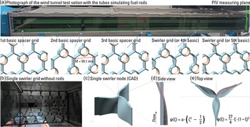
The experimental set-up. (a) Shows the photograph of the wind-tunnel test section with a length $3\,\mathrm{m}$
and inner cross-section
$3\,\mathrm{m}$
and inner cross-section $0.3\times 0.2\,\mathrm{m}$
. There are 5 grids and 20 rods in the grids; air flows from left to right in the figure. The first 3 grids are always the basic spacer grids of alternating nodes of circle shape and tri-star shape. The last one and the penultimate one can be replaced by the swirl-mixing grid with swirling elements at the tri-star nodes, as displayed in the panels (c–e).
$0.3\times 0.2\,\mathrm{m}$
. There are 5 grids and 20 rods in the grids; air flows from left to right in the figure. The first 3 grids are always the basic spacer grids of alternating nodes of circle shape and tri-star shape. The last one and the penultimate one can be replaced by the swirl-mixing grid with swirling elements at the tri-star nodes, as displayed in the panels (c–e).

2. Experimental set-up
2.1. The grid
The spacer and swirl-mixing grids are created by using 3D-printer Prusa Mk 4 from polymerised lactic acid (Inkinen et al. Reference Inkinen, Hakkarainen, Albertsson and Södergøard2011). The grids are connected by using four M6 thread rods inside the wind-tunnel test section. The shape of these grids is inspired by the nuclear fuel assembly for the VVER-440 and VVER-1000 nuclear reactors (Palandi et al. Reference Palandi, Rahimi-Sbo and Rahimi-Esbo2015; Blanc Reference Blanc2022).
Nuclear fuel rods are modelled by using plastic tubes for the food industry of outer diameter $D = 42.2\,\mathrm{mm}$
. These tubes have a smooth black cover with metal reinforcements. A disadvantage is that they are not straight enough and therefore they bend slightly at higher distances past the last grid.
$D = 42.2\,\mathrm{mm}$
. These tubes have a smooth black cover with metal reinforcements. A disadvantage is that they are not straight enough and therefore they bend slightly at higher distances past the last grid.
The mesh parameter is adapted for the diameter of the tubes used. The original VVER-1000 geometry uses a diameter of the rod $D_{\mathrm{real}} = 9.1\,\mathrm{mm}$
and a mesh parameter
$D_{\mathrm{real}} = 9.1\,\mathrm{mm}$
and a mesh parameter $M_{\mathrm{real}} = 12.75\,\mathrm{mm}$
. Thus, our
$M_{\mathrm{real}} = 12.75\,\mathrm{mm}$
. Thus, our $M$
is
$M$
is
 \begin{equation} M = M_{\mathrm{real}}\cdot \frac {D }{ D_{\mathrm{real}}} \approx 59.126\,\mathrm{mm}. \end{equation}
The mesh parameter $M$
is used as the leading dimension unit in our study, similarly to the other studies on grid turbulence (Kurian & Fransson Reference Kurian and Fransson2009; Grzelak & Wierciński Reference Grzelak and Wierciński2015; Bourgoin et al. Reference Bourgoin, Baudet, Kharche, Mordant, Vandenberghe, Sumbekova, Stelzenmuller, Aliseda, Gibert, Roche, Volk, Barois, Caballero, Chevillard, Pinton, Fiabane, Delville, Fourment, Bouha and Peinke2018; Duda et al. Reference Duda, Yanovych and Uruba2020). However, many of the experimental studies regarding flow inside nuclear reactors use the hydraulic diameter
$M$
is used as the leading dimension unit in our study, similarly to the other studies on grid turbulence (Kurian & Fransson Reference Kurian and Fransson2009; Grzelak & Wierciński Reference Grzelak and Wierciński2015; Bourgoin et al. Reference Bourgoin, Baudet, Kharche, Mordant, Vandenberghe, Sumbekova, Stelzenmuller, Aliseda, Gibert, Roche, Volk, Barois, Caballero, Chevillard, Pinton, Fiabane, Delville, Fourment, Bouha and Peinke2018; Duda et al. Reference Duda, Yanovych and Uruba2020). However, many of the experimental studies regarding flow inside nuclear reactors use the hydraulic diameter $D_h$
instead. See e.g. Matozinhos et al. (Reference Matozinhos, Tomaz, Nguyen, dos, André and Hassan2020 Reference Matozinhos, Tomaz, Nguyen and Hassan2021), Nguyen et al. (Reference Nguyen, White, Vaghetto and Hassan2019) and Orosz et al. (Reference Orosz, Magyar, Szerbák, Kacz and Aszódi2022). The hydraulic diameter is defined as
$D_h$
instead. See e.g. Matozinhos et al. (Reference Matozinhos, Tomaz, Nguyen, dos, André and Hassan2020 Reference Matozinhos, Tomaz, Nguyen and Hassan2021), Nguyen et al. (Reference Nguyen, White, Vaghetto and Hassan2019) and Orosz et al. (Reference Orosz, Magyar, Szerbák, Kacz and Aszódi2022). The hydraulic diameter is defined as
 \begin{equation} D_h = 4\cdot \frac {\text{Free cross-sectional area}}{\text{Perimeter of blocked area}} = 4\frac {\tfrac {1}{2}\sqrt {3}M^2 - \tfrac {1}{4}\pi D^2}{\pi D} = D\cdot \left [\frac {2\sqrt {3}}{\pi }\left (\frac {M}{D}\right )^2-1\right ]. \end{equation}
2.1.1. The circle nodes
The odd nodes of the swirler or spacer grids contain a hollow circle, which touches the rods and keeps them in position, see figure 1. The diameter of this circle is equal to the maximum inscribed diameter between the three circles (rods) in a hexagonal lattice. As hexagons consist of equilateral triangles with all the sides of equal length, the inscribed circle radius has to fit the rest of the side to the rod radius, i.e.
 \begin{equation} R_p = s - R_{\mathrm{rod}} = \frac {\sqrt {3}}{3}M - \frac {D}{2}. \end{equation}
2.1.2. The swirl nodes
The swirling element is constructed as a curved plane in local coordinates $(\xi ,\zeta )$
spanning from
$(\xi ,\zeta )$
spanning from $0$
to
$0$
to $1$
. The displacement from the flat plane is described using the function
$1$
. The displacement from the flat plane is described using the function $f(\xi ,\zeta )$
 \begin{equation} f(\xi ,\zeta ) = \underbrace {\frac {27}{4}\cdot \xi \cdot \left (1-\xi \right )^2}_{{\phi (\xi )}} \cdot \underbrace {a \cdot \left (\zeta ^2-\frac {1}{2}\right )}_{{\psi (\zeta )}}, \end{equation}
which is a product of two separated functions $\phi (\xi )$
and
$\phi (\xi )$
and $\psi (\zeta )$
, see figures 1(d) and 1(e) for their projections.
$\psi (\zeta )$
, see figures 1(d) and 1(e) for their projections.
The velocity locally perpendicular to the curved plane is denoted $u_y$
and it is equal
$u_y$
and it is equal $u_y = \frac {\mathrm{d} y}{\mathrm{d} t}$
but the deflection in the perpendicular direction is described by the function
$u_y = \frac {\mathrm{d} y}{\mathrm{d} t}$
but the deflection in the perpendicular direction is described by the function $f(\xi ,\zeta )$
 \begin{equation} u_y = \frac {\mathrm{d} f}{\mathrm{d} t} = \frac {\mathrm{d} f}{\partial \zeta }\frac {\partial \zeta }{\mathrm{d} z}\frac {\mathrm{d} z}{\mathrm{d} t}, \end{equation}
where $\mathrm{d} z / \mathrm{d} t = u_a$
is the axial velocity. Due to the mass conservation across the channel cross-section, one could consider that this component remains constant. This is considered in the general description of turbomachinery (Langston Reference Langston2001; Denton & Pullan Reference Denton and Pullan2012; Klimko & Okresa Reference Klimko and Okresa2016; Lang et al. Reference Lang, Mørck and Woisetschläger2002) and it leads to velocity magnitude increase in curved channels. We have
$\mathrm{d} z / \mathrm{d} t = u_a$
is the axial velocity. Due to the mass conservation across the channel cross-section, one could consider that this component remains constant. This is considered in the general description of turbomachinery (Langston Reference Langston2001; Denton & Pullan Reference Denton and Pullan2012; Klimko & Okresa Reference Klimko and Okresa2016; Lang et al. Reference Lang, Mørck and Woisetschläger2002) and it leads to velocity magnitude increase in curved channels. We have
 \begin{equation} u_y = u_a \cdot \frac {\partial f}{\partial \zeta }\cdot \frac {\partial \zeta }{\partial z} = u_a \cdot 2a\zeta \cdot \phi (\xi )\cdot \frac {1}{h_g} \end{equation}
at the outlet plane ( $\zeta = 1$
) which is equal to
$\zeta = 1$
) which is equal to
 \begin{equation} u_y(\xi ) = 2u_a\frac {a}{h_g}\phi (\xi ) \end{equation}
under the assumption of non-separated flow. Now we can define the Rossby number according to Vignat et al. (Reference Vignat, Durox and Candel2022) as the ratio of axial and azimuthal velocity components
 \begin{equation} \textrm{Ro} = \frac {u_a}{u_y(\xi _{\mathrm{max}})} = \frac {h_g}{2a}, \end{equation}
because $\phi (\xi _{\mathrm{max}}) = 1$
. For the applied dimensions (
$\phi (\xi _{\mathrm{max}}) = 1$
. For the applied dimensions ( $h_g = 20\,\mathrm{mm}$
and
$h_g = 20\,\mathrm{mm}$
and $a = 4\,\mathrm{mm}$
) we get
$a = 4\,\mathrm{mm}$
) we get $\mathrm{Ro} = 5/2$
. Table 1 summarizes the used dimensions.
$\mathrm{Ro} = 5/2$
. Table 1 summarizes the used dimensions.
The characteristics of the lengths, velocities and dimensionless numbers

2.2. Particle image velocimetry
The spatial distribution of the air velocity is measured by using a standard method of particle image velocimetry (PIV) (Tropea et al. Reference Tropea, Yarin and Foss2007; Adrian Reference Adrian2005; Raffel et al. Reference Raffel, Willert, Scarano, Kähler, Wereley and Kompenhans2018). Two Andor Zyla cameras are mounted on a Scheimpflug mount (Arun 2008). The measuring system is double pulse: cameras can distinguish two frames separated down to $\Delta _{T}^{\mathrm{min}}=0.15\,\unicode{x03BC}\mathrm{s}$
; the used value for the current experiment is
$\Delta _{T}^{\mathrm{min}}=0.15\,\unicode{x03BC}\mathrm{s}$
; the used value for the current experiment is $\Delta _T = 40\,{\unicode{x03BC}}{\mathrm{s}}$
(for
$\Delta _T = 40\,{\unicode{x03BC}}{\mathrm{s}}$
(for $U = 20\,{\mathrm{ms}}^{-1}$
). The Andor Zyla cameras have a resolution of
$U = 20\,{\mathrm{ms}}^{-1}$
). The Andor Zyla cameras have a resolution of $2560\times 2160\,\mathrm{pixel^2}$
, pixel depth of
$2560\times 2160\,\mathrm{pixel^2}$
, pixel depth of $12\,\mathrm{bit}$
and pixel pitch of
$12\,\mathrm{bit}$
and pixel pitch of $6.5\,{\unicode{x03BC}}\mathrm{m}$
. The system repeating frequency is
$6.5\,{\unicode{x03BC}}\mathrm{m}$
. The system repeating frequency is $11\,\mathrm{Hz}$
, hence the snapshots are statistically independent. The laser New Wave Solo physically consists of two independently operated lasers with a common optical path, its output colour
$11\,\mathrm{Hz}$
, hence the snapshots are statistically independent. The laser New Wave Solo physically consists of two independently operated lasers with a common optical path, its output colour $\lambda = 532\,\mathrm{nm}$
is obtained from
$\lambda = 532\,\mathrm{nm}$
is obtained from $\lambda _{\mathrm{in}} = 1064\,\mathrm{nm}$
. The laser sheet thickness at the measured area is approximately
$\lambda _{\mathrm{in}} = 1064\,\mathrm{nm}$
. The laser sheet thickness at the measured area is approximately $\sim 1\,\mathrm{mm}$
.
$\sim 1\,\mathrm{mm}$
.
The measured plane lies approximately $\sim 2\,\mathrm{mm}$
behind the exit plane of the wind tunnel. This plane is perpendicular to the rod axis (
$\sim 2\,\mathrm{mm}$
behind the exit plane of the wind tunnel. This plane is perpendicular to the rod axis ( $z$
). Its position is fixed with respect to the rods and the wind tunnel. The position of the system of grids (four grids connected via four thread rods) is moved along the
$z$
). Its position is fixed with respect to the rods and the wind tunnel. The position of the system of grids (four grids connected via four thread rods) is moved along the $z$
-axis (i.e. streamwise) to set the desired distance from the last spacer (or swirler) grid. The following positions are explored:
$z$
-axis (i.e. streamwise) to set the desired distance from the last spacer (or swirler) grid. The following positions are explored: $z = 0.5$
,
$z = 0.5$
, $1$
,
$1$
, $2$
,
$2$
, $3$
and
$3$
and $4\,{M}$
. The first spacer grid in the wind tunnel is fixed to the walls to stabilise the rod tips. Thus, the first inter-grid distance is not constant (otherwise it is
$4\,{M}$
. The first spacer grid in the wind tunnel is fixed to the walls to stabilise the rod tips. Thus, the first inter-grid distance is not constant (otherwise it is $L = 750\,\mathrm{mm} = 12.7\,{M}$
). The rods are made of mat black plastic in order to reduce the reflections.
$L = 750\,\mathrm{mm} = 12.7\,{M}$
). The rods are made of mat black plastic in order to reduce the reflections.
The images are captured and processed within the Dantec Dynamic Studio 6.4. The rod ends are masked, then the minimum of ensemble is subtracted from each pixel (to remove static objects and reflections). Adaptive PIV with a grid step size $32\times 32\,\mathrm{pix}$
and
$32\times 32\,\mathrm{pix}$
and $50 \,\%$
overlap are used to get two-dimensional velocities and Stereo PIV is used to combine vector maps from the both cameras with the calibration matrix.
$50 \,\%$
overlap are used to get two-dimensional velocities and Stereo PIV is used to combine vector maps from the both cameras with the calibration matrix.
2.3. Uncertainty
The uncertainty of the PIV method is a complex issue, and many authors have quantified its magnitude and origins (Charonko & Vlachos Reference Charonko and Vlachos2013; Sciacchitano & Wieneke Reference Sciacchitano and Wieneke2016; Eppink Reference Eppink2020). The total uncertainty arises from several contributions, including particle–flow fidelity, experimental and calibration geometry and the performance of peak-detection algorithms. The Safex particles used in the present study are known to follow the flow faithfully even at supersonic velocities (Scarano Reference Scarano2007; Koschatzky et al. Reference Koschatzky, Moore, Westerweel, Scarano and Boersma2011). The peak-detection uncertainty and peak-height ratio have been analysed by Charonko & Vlachos (Reference Charonko and Vlachos2013), and their method is implemented in the Dantec software. For the current dataset, the resulting displacement uncertainty is typically around $0.2 \,\mathrm{pixel}$
, with several points exceeding
$0.2 \,\mathrm{pixel}$
, with several points exceeding $0.4\,\mathrm{pixel}$
. When related to the mean particle displacement of approximately
$0.4\,\mathrm{pixel}$
. When related to the mean particle displacement of approximately $10 \,\mathrm{pixel}$
, this corresponds to a velocity uncertainty of approximately
$10 \,\mathrm{pixel}$
, this corresponds to a velocity uncertainty of approximately $2\,\%{-}4\, \%$
.
$2\,\%{-}4\, \%$
.
Based on our previous experience (Duda et al. Reference Duda, Yanovych and Uruba2025), the dominant contribution to the overall uncertainty is the calibration accuracy. In the present case, the mean reprojection error is $0.38\,\mathrm{pixel}$
, which again corresponds to roughly
$0.38\,\mathrm{pixel}$
, which again corresponds to roughly $3.8\, \%$
uncertainty in the velocity. The alignment between the measurement plane and the calibration plane is one of the most critical aspects of stereo-PIV, as emphasised by Eppink (Reference Eppink2020). In our procedure, the calibration target is first positioned at the intended measurement location, the cameras are focused on the target, the sensors are protected and the laser sheet is then carefully aligned to illuminate the front surface of the target while maximising the visibility of dust-particle shadows. Any residual misalignment may not only bias the measured velocities but can also introduce artificial velocity gradients, which would directly affect the inferred vortex properties (Eppink Reference Eppink2020). The influence of measurement uncertainty on the fitted vortex parameters has not yet been systematically investigated.
$3.8\, \%$
uncertainty in the velocity. The alignment between the measurement plane and the calibration plane is one of the most critical aspects of stereo-PIV, as emphasised by Eppink (Reference Eppink2020). In our procedure, the calibration target is first positioned at the intended measurement location, the cameras are focused on the target, the sensors are protected and the laser sheet is then carefully aligned to illuminate the front surface of the target while maximising the visibility of dust-particle shadows. Any residual misalignment may not only bias the measured velocities but can also introduce artificial velocity gradients, which would directly affect the inferred vortex properties (Eppink Reference Eppink2020). The influence of measurement uncertainty on the fitted vortex parameters has not yet been systematically investigated.
3. Results
3.1. Results: mean field
Figure 2 shows the mean velocity fields. Averaging is performed over the ensemble of $500$
independent snapshots. The repeating frequency of the PIV system is
$500$
independent snapshots. The repeating frequency of the PIV system is $11 \,\mathrm{Hz}$
, i.e. at velocity
$11 \,\mathrm{Hz}$
, i.e. at velocity $U=20\,{\mathrm{ms}}^{-1}$
the fluid travels around
$U=20\,{\mathrm{ms}}^{-1}$
the fluid travels around $1.8\,\mathrm{m}$
between consecutive snapshots, which is definitely over the size of any possible flow structures within the geometry studied (Duda & Uruba Reference Duda and Uruba2018; Yanovych et al. Reference Yanovych, Duda and Uruba2021).
$1.8\,\mathrm{m}$
between consecutive snapshots, which is definitely over the size of any possible flow structures within the geometry studied (Duda & Uruba Reference Duda and Uruba2018; Yanovych et al. Reference Yanovych, Duda and Uruba2021).
The measured mean velocity field. Colour represents the $w$
velocity component along the
$w$
velocity component along the $z$
axis (i.e. parallel to the rods, perpendicular to measuring plane). Vectors represent the in-plane velocities. The first column displays the case of basic spacer grids (b.g.) which consists of alternating circle nodes and tri-star nodes. The second column shows the data when the last grid is the swirl grid (s.g.), where the swirling elements are at the tri-star nodes, the circle nodes remain the same as for the basic grid. The third column is the case of two swirl grids; note that the upstream grid has exchanged circle and tri-star nodes, additionally, the swirling elements are mirrored. The right column displays the comparative case of a single swirl grid with no rods in between to compare with the behaviour of free vortices, as have been studied by Duda & yanovych (Reference Duda and Yanovych2024).
$z$
axis (i.e. parallel to the rods, perpendicular to measuring plane). Vectors represent the in-plane velocities. The first column displays the case of basic spacer grids (b.g.) which consists of alternating circle nodes and tri-star nodes. The second column shows the data when the last grid is the swirl grid (s.g.), where the swirling elements are at the tri-star nodes, the circle nodes remain the same as for the basic grid. The third column is the case of two swirl grids; note that the upstream grid has exchanged circle and tri-star nodes, additionally, the swirling elements are mirrored. The right column displays the comparative case of a single swirl grid with no rods in between to compare with the behaviour of free vortices, as have been studied by Duda & yanovych (Reference Duda and Yanovych2024).

The mean in-plane velocity components ( $u$
and
$u$
and $v$
) are displayed through vectors. Only every fourth vector is displayed in order to avoid too many lines in the figure. The streamwise velocity component
$v$
) are displayed through vectors. Only every fourth vector is displayed in order to avoid too many lines in the figure. The streamwise velocity component $w$
is displayed via colour.
$w$
is displayed via colour.
The spatial distribution of streamwise velocity shows values around and higher than the reference velocity $U$
. This is the effect of boundary layers on the rod walls. The boundary layers are not directly visible in the figure, because they are under the mask (white area) covering the fuel rods and the near neighbourhood, as described in § 2.2.
$U$
. This is the effect of boundary layers on the rod walls. The boundary layers are not directly visible in the figure, because they are under the mask (white area) covering the fuel rods and the near neighbourhood, as described in § 2.2.
Note the jets formed past the circle nodes of the spacer grid and visible as spots of higher streamwise velocity (brown spots in figure 2). They are apparent in all explored cases. Past the other nodes (of tri-star shape or with the swirling element), this jet is weaker and it is suppressed by the wake past the walls (straight or twisted). This “shadow” of walls is apparent up to $z/M\approx 2$
. It is twisted in the cases with swirling elements.
$z/M\approx 2$
. It is twisted in the cases with swirling elements.
In the case of an empty grid (the right column in figure 2), the lowest observed velocity is located past the connections of the circle nodes to the walls. The wake past circular element of the grid is deeper at the beginning, but it recovers faster than the rotating wake past the swirler element.
Figure 3 displays the mean in-plane vorticity (along the $z$
-axis) calculated from the in-plane velocity components (
$z$
-axis) calculated from the in-plane velocity components ( $u$
and
$u$
and $v$
) by using the second-order differentiation scheme (Habchi et al. Reference Habchi, Lemenand, Valle and Peerhossaini2010; Wu et al. Reference Wu, Ma and Zhou2006). There is no significant vorticity signal in the case of a basic spacer grid (the left column in figure 3); the observed signal at the edge of masks originates from the experimental noise and does not have physical significance. In the swirling cases, there is a spot of vorticity persisting over the entire explored range of
$v$
) by using the second-order differentiation scheme (Habchi et al. Reference Habchi, Lemenand, Valle and Peerhossaini2010; Wu et al. Reference Wu, Ma and Zhou2006). There is no significant vorticity signal in the case of a basic spacer grid (the left column in figure 3); the observed signal at the edge of masks originates from the experimental noise and does not have physical significance. In the swirling cases, there is a spot of vorticity persisting over the entire explored range of $z$
. At the adjacent boundary layers, one can observe the spots of counter-oriented vorticity originating from the in-plane shear. Note that vorticity is sensitive not only to vortices, but to shear as well (Pope Reference Pope2000).
$z$
. At the adjacent boundary layers, one can observe the spots of counter-oriented vorticity originating from the in-plane shear. Note that vorticity is sensitive not only to vortices, but to shear as well (Pope Reference Pope2000).
The in-plane vorticity component is calculated by using the second-order differentiation scheme on the PIV data grid.

If the upstream grid contains swirling elements at complementary nodes, then weaker vortices appear even in the distance over $13\,{M}$
. This suggests that the vortices generated by swirling elements are stable coherent structures with long lifetime similar to wing-tip vortices (Ansaripour et al. Reference Ansaripour, Dafsari, Yu, Choi and Lee2023; Bardera et al. Reference Bardera, Barroso and Matías2022; Dghim et al. Reference Dghim, Ben Miloud, Ferchichi and Fellouah2021). Therefore, it makes sense to ask: How do those vortices develop, how do they meander and so on?
$13\,{M}$
. This suggests that the vortices generated by swirling elements are stable coherent structures with long lifetime similar to wing-tip vortices (Ansaripour et al. Reference Ansaripour, Dafsari, Yu, Choi and Lee2023; Bardera et al. Reference Bardera, Barroso and Matías2022; Dghim et al. Reference Dghim, Ben Miloud, Ferchichi and Fellouah2021). Therefore, it makes sense to ask: How do those vortices develop, how do they meander and so on?
3.2. Results: individual vortices
Individual vortices are detected on each snapshot by directly fitting the instantaneous two-dimensional velocity field. The Nelder-Mead Amoeba fitting algorithm (Nelder & Mead Reference Nelder and Mead1965) is implemented according to the book Numerical Recipes (Press et al. Reference Press, Teukolsky, Vetterling and Flannery2007). There are four fitting parameters for each vortex: $x$
-position,
$x$
-position, $y$
-position, circumferential velocity
$y$
-position, circumferential velocity $G = \Gamma / (2\pi R)$
and the vortex core radius
$G = \Gamma / (2\pi R)$
and the vortex core radius $R$
. Here,
$R$
. Here, $G$
is used instead of
$G$
is used instead of $\Gamma$
due to the better fitting stability and clearer dimension (
$\Gamma$
due to the better fitting stability and clearer dimension ( $\Gamma$
has a composite dimension dependent on two normalisations: velocity and length scale). Of course, it would be possible to add more parameters connected with the streamwise velocity deficit at the core or with the vortex deformation. However, we prefer a simpler approach due to the famous statement by John von Neumann: “by using four parameters an elephant can be fitted”, which has been demonstrated by Meyer et al. (Reference Meyer, Khairy and Howard2010).
$\Gamma$
has a composite dimension dependent on two normalisations: velocity and length scale). Of course, it would be possible to add more parameters connected with the streamwise velocity deficit at the core or with the vortex deformation. However, we prefer a simpler approach due to the famous statement by John von Neumann: “by using four parameters an elephant can be fitted”, which has been demonstrated by Meyer et al. (Reference Meyer, Khairy and Howard2010).
Decreasing the number of fitting parameters increases the stability of the process. The radius of the vortices generated at the upstream grid is strictly set to $R = 0.1\,{M}$
, which is close to an average value observed at the stronger vortices – see figure 5. Locking one variable in the Amoeba algorithm is achieved by setting the corresponding vertex of the simplex. The simplex is thus degenerated in the corresponding dimension and it cannot evolve out of the locked value.
$R = 0.1\,{M}$
, which is close to an average value observed at the stronger vortices – see figure 5. Locking one variable in the Amoeba algorithm is achieved by setting the corresponding vertex of the simplex. The simplex is thus degenerated in the corresponding dimension and it cannot evolve out of the locked value.
The minimised variable is the energy of the two-dimensional velocity field after subtracting the velocity field generated by the vortex of such parameters. When the energy of the residual velocity field reaches a minimum, the velocity field of this vortex is subtracted, vortex parameters are saved into a file and the next vortex starts to be fitted. More details about this process can be found in our previous works (Duda Reference Duda, Šimurda and Bodnár2020, Reference Duda, Šimurda and Bodnár2021
a, b). In the mentioned studies, significant attention is paid to the question of starting parameters. In the current experiment, the vortices are always in a similar location, therefore, we can significantly shorten the search algorithm because, as stated by Milne (Reference Milne1926), when we catch something, the best way is to start digging just where it is. Therefore, we use an ansatz constructed at the mean velocity field (figure 2). The main advantage is that the same index is always given to the vortex in a specified place; therefore, we can construct new vortex properties: e.g. the displacement from the equilibrium position $\Delta$
and explore its behaviour.
$\Delta$
and explore its behaviour.
Fits of the downstream evolution of vortex properties. Here, $\Gamma _0/(UM)$
is the circulation at virtual position
$\Gamma _0/(UM)$
is the circulation at virtual position $z=0$
;
$z=0$
; $\lambda /M$
is the decay length of vortex circulation;
$\lambda /M$
is the decay length of vortex circulation; $\Delta _0/M$
is the meandering amplitude at
$\Delta _0/M$
is the meandering amplitude at $z=0$
, with values multiplied by
$z=0$
, with values multiplied by $1000$
;
$1000$
; $\Lambda /M$
is the growth length of the meandering amplitude
$\Lambda /M$
is the growth length of the meandering amplitude

3.2.1. Downstream development of vortex circulation
The circulation at figure 4 is not fitted directly, it is constructed as
 \begin{equation} \Gamma = 2\pi \cdot G\cdot R, \end{equation}
where $G$
is the circumferential velocity (this is fitted directly) and
$G$
is the circumferential velocity (this is fitted directly) and $R$
is the vortex core radius. Here,
$R$
is the vortex core radius. Here, $R$
is fitted for the 5 primary vortices produced at the last swirl grid which are observable in figure 3 as blue-white spots. The older vortices produced at the upstream grid at adjacent nodes are much weaker (brown spots in figure 3 – the third column). To stabilise the fitting procedure, the vortex core radius is locked to the value of the vortex in the mean field, but only for vortices generated at the upstream grid.
$R$
is fitted for the 5 primary vortices produced at the last swirl grid which are observable in figure 3 as blue-white spots. The older vortices produced at the upstream grid at adjacent nodes are much weaker (brown spots in figure 3 – the third column). To stabilise the fitting procedure, the vortex core radius is locked to the value of the vortex in the mean field, but only for vortices generated at the upstream grid.
The streamwise development of the mean circulations $\Gamma$
of the vortex ensemble. The exponential decay fit is displayed for the single grid and the case without rods.
$\Gamma$
of the vortex ensemble. The exponential decay fit is displayed for the single grid and the case without rods.

The circulation decays exponentially as suggested by the Helmholtz (Reference Helmholtz1858, Reference Helmholtz1868) theorem with added viscosity, because the time derivative of $\Gamma$
 \begin{equation} \mathrm{d} \Gamma /\mathrm{d} t \sim \nu \cdot \nabla ^2 \omega, \end{equation}
but $\omega$
is proportional to
$\omega$
is proportional to $\Gamma$
, which does not depend on the coordinate, thus the
$\Gamma$
, which does not depend on the coordinate, thus the $\nabla ^2$
operator does not affect it much. Since for typical vortex profiles with decreasing
$\nabla ^2$
operator does not affect it much. Since for typical vortex profiles with decreasing $\omega$ $\nabla ^2\omega$
is negative, thus
$\nabla ^2\omega$
is negative, thus $\mathrm{d} \Gamma /\mathrm{d} t \sim \Gamma$
, which is typical for exponential decay. We do not try to find the decay constant analytically as we did in Duda & Yanovych (Reference Duda and Yanovych2024), because, in the current case, boundary layers are presented and we can expect that they will suck the energy from vortex in an unpredictable way. However, the importance of the energy leak due to boundary layers is apparent from the different slope of circulation decay in the free (green line in figure 4) or constrained (blue line at figure 4) case. If we consider the decay in the form
$\mathrm{d} \Gamma /\mathrm{d} t \sim \Gamma$
, which is typical for exponential decay. We do not try to find the decay constant analytically as we did in Duda & Yanovych (Reference Duda and Yanovych2024), because, in the current case, boundary layers are presented and we can expect that they will suck the energy from vortex in an unpredictable way. However, the importance of the energy leak due to boundary layers is apparent from the different slope of circulation decay in the free (green line in figure 4) or constrained (blue line at figure 4) case. If we consider the decay in the form
 \begin{equation} \Gamma (z) \sim e^{-z/\lambda }, \end{equation}
then the $\lambda$
values for the studied cases are listed in table 2.
$\lambda$
values for the studied cases are listed in table 2.
The decay length $\lambda$
past a single swirl grid or past two swirl grids does not differ much (in figure 4 we did not draw that line). In contrast, the decay length in the case without fuel rods is significantly higher (15 vs. 11), suggesting that the difference is what takes the interaction with boundary layers. The older vortices generated at the upstream grid display a shorter decay length. This can be caused by the larger meandering amplitude and thus stronger interaction with the boundary layers at fuel rods.
$\lambda$
past a single swirl grid or past two swirl grids does not differ much (in figure 4 we did not draw that line). In contrast, the decay length in the case without fuel rods is significantly higher (15 vs. 11), suggesting that the difference is what takes the interaction with boundary layers. The older vortices generated at the upstream grid display a shorter decay length. This can be caused by the larger meandering amplitude and thus stronger interaction with the boundary layers at fuel rods.
In figure 4 we extrapolated the decay line of the single swirl grid over the distance $L$
between grids. This displays how it would look if the function continued ideally – see the bottom blue line in figure 4. The observed circulations lie under this curve; and they decay faster (
$L$
between grids. This displays how it would look if the function continued ideally – see the bottom blue line in figure 4. The observed circulations lie under this curve; and they decay faster ( $\lambda _{\mathrm{upstream}}=7.5$
in contrast to
$\lambda _{\mathrm{upstream}}=7.5$
in contrast to $\lambda _{\mathrm{1sg}} =11$
). We think that this difference is like a “price” of passing through the circle node of the next swirl grid. But some quantitative conclusions cannot be made from this comparison, because the extrapolation is too extensive – a measurement before the next grid would be needed, but it is technically impossible with the current apparatus.
$\lambda _{\mathrm{1sg}} =11$
). We think that this difference is like a “price” of passing through the circle node of the next swirl grid. But some quantitative conclusions cannot be made from this comparison, because the extrapolation is too extensive – a measurement before the next grid would be needed, but it is technically impossible with the current apparatus.
3.2.2. Vortex core radii
Average radii of vortex cores are displayed in figure 5 as a function of $z$
. Note that the radii of weaker vortices produced at the upstream grid are locked (as have been discussed above), and thus they are not displayed in figure 5.
$z$
. Note that the radii of weaker vortices produced at the upstream grid are locked (as have been discussed above), and thus they are not displayed in figure 5.
Vortex core radii. Note that the vortices from the upstream grid (denoted in yellow in the other graphs) are fitted with a locked core radius in order to increase the fitting procedure stability. Hence they are not displayed here.

We see similar values of $R$
for both constrained cases: almost constant with very slow decrease. This is probably caused by boundary layers (BL). As BL produce turbulence on a length scale smaller than the discussed stream vortices, the envelope of these vortices is depressed, leading to compression of the vortex core (Amromin Reference Amromin2007). Vortices in the case without fuel rods (green circles) grow in size as expected due to the spreading of the vorticity, as discussed in the past by Helmholtz (Reference Helmholtz1858, Reference Helmholtz1868) and many others (Oseen Reference Oseen1912; Batchelor Reference Batchelor1964; Alekseenko et al. Reference Alekseenko, Kuibin and Okulov2003).
$R$
for both constrained cases: almost constant with very slow decrease. This is probably caused by boundary layers (BL). As BL produce turbulence on a length scale smaller than the discussed stream vortices, the envelope of these vortices is depressed, leading to compression of the vortex core (Amromin Reference Amromin2007). Vortices in the case without fuel rods (green circles) grow in size as expected due to the spreading of the vorticity, as discussed in the past by Helmholtz (Reference Helmholtz1858, Reference Helmholtz1868) and many others (Oseen Reference Oseen1912; Batchelor Reference Batchelor1964; Alekseenko et al. Reference Alekseenko, Kuibin and Okulov2003).
3.2.3. Vortex meandering
Vortex meandering, sometimes referred as wandering (Bailey & Tavoularis Reference Bailey and Tavoularis2008; Edstrand et al. Reference Edstrand, Davis, Schmid, Taira and Cattafesta2016), is the motion of a vortex with respect to its equilibrium position. It is often expressed as the standard deviation of the vortex position along a single coordinate (e.g. $y$
), if this coordinate makes a good sense (e.g. past the tip of an airfoil, then this coordinate is perpendicular to both the stream and wing span). One such experiment was performed by Bailey and Tavoularis (Reference Bailey and Tavoularis2008); they used a pair of hot-wire probes to calculate the position of the vortex using the very complex method of Devenport et al. (Reference Devenport, Rife, Liapis and Follin1996).
$y$
), if this coordinate makes a good sense (e.g. past the tip of an airfoil, then this coordinate is perpendicular to both the stream and wing span). One such experiment was performed by Bailey and Tavoularis (Reference Bailey and Tavoularis2008); they used a pair of hot-wire probes to calculate the position of the vortex using the very complex method of Devenport et al. (Reference Devenport, Rife, Liapis and Follin1996).
Our method to estimate the vortex meandering amplitude is simpler and straighter: the average vortex position of each vortex is calculated in the Field of View (FoV). Matching the vortex in one snapshot to the corresponding vortices in the other snapshots is simple due to the fitting from the ansatz calculated from the ensemble-averaged velocity field. The meandering amplitude $\Delta _{i,t}$
of each vortex of index
$\Delta _{i,t}$
of each vortex of index $i$
(index of the vortex within the FoV) at time
$i$
(index of the vortex within the FoV) at time $t$
is then calculated as a distance from its time-averaged position
$t$
is then calculated as a distance from its time-averaged position
 \begin{equation} \Delta _{i,t} = \sqrt {\left (x_{i,t} - \left \langle x_i\right \rangle _t\right )^2 + \left (y_{i,t} - \left \langle y_i\right \rangle _t\right )^2}. \end{equation}
Figure 6 displays the averaged ensemble and index value
 \begin{equation} \Delta = \Big \langle \left \langle \Delta _{i,t}\right \rangle _t\Big \rangle _i, \end{equation}
where the order of averaging does not matter due to linearity of averaging (there is always the same number of vortices in each snapshot).
The meandering amplitude for the studied cases.

Figure 6 displays the meandering amplitude with the downstream distance. The meandering amplitude past the empty swirl grid is the lowest; the presence of fuel rods increases the meandering amplitude. The presence of vortices in the circle nodes increases the meandering amplitude even more. Naturally, the meandering of older vortices is stronger, and still grows in the observed region.
Assuming an exponential growth of $\langle \Delta \rangle$
 \begin{equation} \langle \Delta (z)\rangle \approx \Delta _0\cdot e^{z/\Lambda }, \end{equation}
where the fitting is performed as a linear fit of the logarithm of $\Delta$
. Meandering amplitudes
$\Delta$
. Meandering amplitudes $\Delta _0$
and the growth rates
$\Delta _0$
and the growth rates $\Lambda$
are listed in table 2.
$\Lambda$
are listed in table 2.
3.2.4. Correlations of single vortex properties
Figure 7 shows the correlation of the vortex circumferential velocity $G$
and the meandering amplitude
$G$
and the meandering amplitude $\Delta$
. The correlation coefficient is calculated simply by using the Pearson formula
$\Delta$
. The correlation coefficient is calculated simply by using the Pearson formula
 \begin{equation} r_{G\Delta } = \frac {\Big \langle \left (G_{it}-\left \langle G\right \rangle _{it}\right )\cdot \left (\Delta _{it}-\left \langle \Delta \right \rangle _{it}\right ) \Big \rangle _{it}}{\sigma [G]\cdot \sigma [\Delta ]}, \end{equation}
where $\sigma [G], \sigma [\Delta ]$
are standard deviations of the corresponding ensembles. This correlation is observed to be negative in all of the cases, suggesting that as the vortex moves far from equilibrium, it loses some energy and thus decreases its velocity. However, this correlation is rather weak, between
$\sigma [G], \sigma [\Delta ]$
are standard deviations of the corresponding ensembles. This correlation is observed to be negative in all of the cases, suggesting that as the vortex moves far from equilibrium, it loses some energy and thus decreases its velocity. However, this correlation is rather weak, between $-40\,\%$
and
$-40\,\%$
and $0$
. The weakest correlation is expected for the vortices past an empty grid, because there are no BL, approaching which may lead to energy loss. The observed downstream development (strong, then weak and then gets stronger again) can be explained at later stages (
$0$
. The weakest correlation is expected for the vortices past an empty grid, because there are no BL, approaching which may lead to energy loss. The observed downstream development (strong, then weak and then gets stronger again) can be explained at later stages ( $2{-}4\,{M}$
) as follows: the more meandering vortex approaches closer to the BL, which drains its energy. As the meandering amplitude increases downstream (compare with figure 6), the approach to the BL is stronger.
$2{-}4\,{M}$
) as follows: the more meandering vortex approaches closer to the BL, which drains its energy. As the meandering amplitude increases downstream (compare with figure 6), the approach to the BL is stronger.
Correlation coefficient of the vortex circumferential velocity $G_i$
and the actual displacement from the equilibrium position
$G_i$
and the actual displacement from the equilibrium position $\Delta _i$
.
$\Delta _i$
.

3.2.5. Correlation of neighbouring vortices
From the point of view of cooling enhancement within the nuclear fuel assembly, very interesting is the question of whether there can exist coherent structures across the neighbouring coolant channels, whose decay may homogenise the cooling along the axial direction. The current experimental arrangement together with the unique algorithm for individual vortex detection can help answer this question, at least in the case studied here, of a swirl grid generating an axial vortex at each second node with Rossby number $5/2$
. Figure 9 shows the downstream development of the correlation of the circumferential velocities of neighbouring vortices. In the case of 2 swirl grids characterised by 2 populations of vortices, we can explore not only mutual correlation of neighbouring main vortices (brown
$5/2$
. Figure 9 shows the downstream development of the correlation of the circumferential velocities of neighbouring vortices. In the case of 2 swirl grids characterised by 2 populations of vortices, we can explore not only mutual correlation of neighbouring main vortices (brown $\diamond$
in graphs), but also the correlation of the main vortex with the weaker one (yellow
$\diamond$
in graphs), but also the correlation of the main vortex with the weaker one (yellow $\Delta$
) and the mutual correlation of the two older and weaker vortices, which have already enough time to start communicating (maroon
$\Delta$
) and the mutual correlation of the two older and weaker vortices, which have already enough time to start communicating (maroon $\nabla$
).
$\nabla$
).
The correlation of circumferential velocity in figure 9 shows weak correlation of older vortices as well as weak correlation of the vortices in the free environment. However, the constraint inside the interrod channels seems to introduce some weak correlation between the main vortices. This correlation is still $\lt 30\,\%$
with maximum at
$\lt 30\,\%$
with maximum at $z = 2\,{M}$
.
$z = 2\,{M}$
.
What causes this correlation? A natural hypothesis is the meandering – a vortex moved out of the central point pushes the fluid in the narrow channel, which then influences the vortex in neighbouring channel. But, the correlation of meandering amplitudes of neighbouring vortices in figure 8(top left) displays effectively zero correlation in all cases and at all explored distances. The Pearson formula (3.7) compares the departure from the mean value, in other words, $r_{\Delta \Delta }$
would report strong correlation if the meandering amplitudes of both compared vortices are larger or smaller than the mean meandering amplitude at the same time. Additionally,
$r_{\Delta \Delta }$
would report strong correlation if the meandering amplitudes of both compared vortices are larger or smaller than the mean meandering amplitude at the same time. Additionally, $\Delta$
does not contain information about the direction.
$\Delta$
does not contain information about the direction.
Correlation of the displacement from mean position for neighbouring vortices. Top left: absolute value of displacement – meandering amplitude; top right: displacement in the $x$
-direction; bottom left: displacement in the
$x$
-direction; bottom left: displacement in the $y$
-direction, bottom right: correlation between the
$y$
-direction, bottom right: correlation between the $x$
-displacement of the left vortex and the
$x$
-displacement of the left vortex and the $y$
-displacement of the right one.
$y$
-displacement of the right one.

Correlation of the circumferential velocities $G$
of the neighbouring vortices. For the case of two swirl grids, more pairs are introduced: the correlation between the nearest main vortices (from the last grid), the correlation between the main vortex and the nearest older vortex and the correlation between the neighbouring vortices from the upstream grid.
$G$
of the neighbouring vortices. For the case of two swirl grids, more pairs are introduced: the correlation between the nearest main vortices (from the last grid), the correlation between the main vortex and the nearest older vortex and the correlation between the neighbouring vortices from the upstream grid.

However, if we compare the meandering with respect to the direction, see the other panels of figure 8, we do not observe a strong signal in any case. Only the weaker vortices produced at the upstream grid display some weak anticorrelation around $20\,\%$
in their
$20\,\%$
in their $x$
and
$x$
and $y$
-positions. This suggests a “dancing” of vortices in the sense that they move towards or away from each other and, if one moves up, the second moves down. However, the correlation is rather small and exists only at the pair of vortices produced at the upstream grid, which are already older, and thus they have had a longer time for interaction. The “newborn” vortices do not display significant correlation for any of the explored cases (single swirl grid, second swirl grid or even the case without fuel rods).
$y$
-positions. This suggests a “dancing” of vortices in the sense that they move towards or away from each other and, if one moves up, the second moves down. However, the correlation is rather small and exists only at the pair of vortices produced at the upstream grid, which are already older, and thus they have had a longer time for interaction. The “newborn” vortices do not display significant correlation for any of the explored cases (single swirl grid, second swirl grid or even the case without fuel rods).
The correlation of vortex positions is observed to be small, while the correlation of velocities of neighbouring vortices is up to $30\,\%$
at its maximum. Another effect to be checked is the streamwise velocity at vortex centres. In other words, the evidence of a long-range coherent structure formed across the interrod channels. This correlation is displayed in Figure 10 and we see a positive, but small, correlation in almost all cases.
$30\,\%$
at its maximum. Another effect to be checked is the streamwise velocity at vortex centres. In other words, the evidence of a long-range coherent structure formed across the interrod channels. This correlation is displayed in Figure 10 and we see a positive, but small, correlation in almost all cases.
Correlation of the energies saved during the fitting procedure by the adjacent vortices. In the case of a single swirl grid, the correlated vortices are that at adjacent nodes; in the case of 2 swirl grids, the correlated vortices are the weaker upstream vortex and the main one (yellow $\Delta$
) or the neighbouring upstream vortices (maroon
$\Delta$
) or the neighbouring upstream vortices (maroon $\nabla$
).
$\nabla$
).

4. Conclusion
In this study, we apply the ideas of recent research (Duda & Yanovych Reference Duda and Yanovych2024) showing delayed turbulence decay for a vortex-inducing grid. We adapted the standard spacer grid for the VVER-1000 nuclear reactor in such a way that it generates vortices by swirling the flow at a Rossby number of $2.5$
at each second node of the grid. The isothermal velocity field is mapped at distances of
$2.5$
at each second node of the grid. The isothermal velocity field is mapped at distances of $0.5, 1, 2, 3$
and
$0.5, 1, 2, 3$
and $4\times$
the interrod distance
$4\times$
the interrod distance $M$
from the swirl grid by using a standard tool of PIV.
$M$
from the swirl grid by using a standard tool of PIV.
We have observed stable vortices induced in the interrod channels past swirler nodes. Their presence increases the standard deviation of vorticity even in the areas that are not directly influenced by the vortices. Vortices created at the upstream grid are weaker, but clearly recognisable.
The method of individual vortex detection (Duda 2021b) allows us to analyse properties of individual vortices. The following observations have been made:
-
i. The vortex circulations decrease faster in between the BL at fuel rods in comparison with the unconstrained case. The passage through the next grid accelerates the circulation decay even more.
-
ii. The size of the vortex core is not growing when constrained (in the free case, it grows).
-
iii. The meandering amplitude of vortices grows exponentially with downstream distance in the explored region. The meandering is slightly stronger in the constrained case than in the free case. Adding an upstream grid amplifies meandering even more.
-
iv. There is small anticorrelation ( $\sim -15\,\%$
) between the vortex circumferential velocity and meandering amplitude (vortex is further than usual from its equilibrium position
$\Leftrightarrow$
the vortex rotates less). This anticorrelation is weaker for the free case.
$\sim -15\,\%$
) between the vortex circumferential velocity and meandering amplitude (vortex is further than usual from its equilibrium position
$\Leftrightarrow$
the vortex rotates less). This anticorrelation is weaker for the free case. -
v. The circumferential velocities of neighbouring vortices correlate (
$\sim +20\,\%$
) in the case of main vortices with fuel rods. For the older or free ones, no correlation is observed. -
vi. There is no distinct correlation between the vortex positions. The strongest signal is observable for upstream vortices in their
$x$
and
$y$
-positions. -
vii. Vortex energies measured as the difference between the original velocity field and the residual velocity field displays the same profile as the correlation of circumferential velocities.


The fact that neighbouring vortices correlate in their velocities and energies, but not in positions, is a mystery, which has to be explored during future research employing, not only careful experiments at different Rossby numbers and/or spacings between swirler elements, but also numerical simulations of vortex filaments (Dergachev et al. Reference Dergachev, Marchevsky and Shcheglov2019; Hänninen & Baggaley Reference Hänninen and Baggaley2014).
Supplementary material
The supplementary material for this article can be found at https://doi.org/10.17632/ds8c6837x8.1.
Data availability statement
Data in the form of vector fields are available at the Mendeley Data repository under doi https://doi.org/10.17632/ds8c6837x8.1. As the original image data are too big to be in an online repository, they are stored at HDD at the University of West Bohemia in Pilsen and will be made available on demand.
Author contributions
M.D. and D.D. performed the measurement; V.J. and D.D. prepared the grid geometry; D.D. and V.Y. analysed the data; D.D. and A.M. wrote the manuscript; I.K.VS. wrote the program for the vortex dynamics; K.K. controlled the English quality; V.U. supervised the team.
Funding statement
The authors acknowledge support of the University of West Bohemia, Faculty of Mechanical Engineering, Department of Power System Engineering via project SGS-2025-013 `Research and Development of Modern Power Machines and “Facilities”.
Competing interests
The authors declare no conflicts of interest.
Ethical standards
The research meets all ethical guidelines, including adherence to the legal requirements of the country.


 Open access