


1. Introduction
Stock markets are excessively volatile and subject to strong boom-bust dynamics. As is well known, the vagaries of stock markets can have serious consequences for the real economy. The Great Depression and the Global Financial Crises are just two particularly tragic examples. See Galbraith (Reference Galbraith1994), Reinhart and Rogoff (Reference Reinhart and Rogoff2009), Kindleberger and Aliber (Reference Kindleberger and Aliber2011) and Shiller (Reference Shiller2015) for detailed historical accounts. Fortunately, models with heterogeneous interacting agents have proven to be useful frameworks for better understanding the complex behavior of stock markets. This line of research, pioneered by Zeeman (Reference Zeeman1974), Beja and Goldman (Reference Beja and Goldman1980), Day and Huang (Reference Day and Huang1990), Chiarella (Reference Chiarella1992), Lux (Reference Lux1995) and Brock and Hommes (Reference Brock and Hommes1998), studies the interplay between chartists, fundamentalists and market makers. Chartists are typically modeled as traders who bet on a continuation of the current stock price trend.Footnote 1 Their positive feedback trading tends to destabilize stock markets. Fundamental traders believe in mean reversion. Buying (selling) undervalued (overvalued) stocks tends to stabilize stock markets. Market makers mediate the transactions of chartists and fundamentalists out of equilibrium, adjusting stock prices to reflect current excess demand. Faced with positive (negative) excess demand, market makers raise (lower) the stock price. These three model components result in dynamical systems whose mathematical and numerical analysis advances our understanding of the functioning of stock markets. See Dieci and He (Reference Dieci, He, Dieci and He2018) and Axtell and Farmer (Reference Axtell and Farmer2024) for reviews.
To obtain clear-cut analytical insights into the functioning of stock markets, a branch of this line of research has started to investigate more stylized representations of stock markets. For instance, Huang and Day (Reference Huang, Day, Huang and Day1993), Tramontana et al. (Reference Tramontana, Westerhoff and Gardini2010, Reference Tramontana, Westerhoff and Gardini2013) and Jungeilges et al. (Reference Jungeilges, Maklakova and Perevalova2021, Reference Jungeilges, Maklakova and Perevalova2022) show that the trading behavior of heterogeneous speculators, who rely on piecewise-linear trading rules, may give rise to complex bull and bear market dynamics. The dynamics of this “first-generation” class of stock market models is due to one-dimensional piecewise-linear maps. More recently, Anufriev et al. (Reference Anufriev, Gardini and Radi2020), Dieci et al. (Reference Dieci, Gardini and Westerhoff2022) and Gardini et al. (Reference Gardini, Radi, Schmitt, Sushko and Westerhoff2022a,b,c) have initiated a “second-generation” class of stock market models in which two-dimensional piecewise-linear maps govern stock market dynamics. This new approach not only allows for a richer modeling of the trading behavior of stock market participants—its mathematical properties, which have been little studied, yield insights that may ultimately help policymakers design more efficient stock markets.Footnote 2 In this paper, which belongs to the latter research area, we generalize the stock market model by Gardini et al. (Reference Gardini, Radi, Schmitt, Sushko and Westerhoff2022c). Moreover, we provide a thorough analytical and numerical treatment of the dynamic properties of our new framework. In doing so, we hope to advance this important line of research in both economic and mathematical terms.
Let us briefly recall the model setup by Gardini et al. (Reference Gardini, Radi, Schmitt, Sushko and Westerhoff2022c). Their stock market model is populated by market makers, chartists and fundamentalists. Market makers quote stock prices with respect to speculators’ excess demand, chartists bet on the persistence of stock price trends, and fundamentalists presume that stock prices revert toward their fundamental values. However, fundamentalists’ perception of the stock market’s fundamental value is subject to animal spirits. Gardini et al. (Reference Gardini, Radi, Schmitt, Sushko and Westerhoff2022c) consider two generic sentiment states. Fundamentalists optimistically (pessimistically) believe in a relatively high (low) fundamental value when the stock market increases (decreases). A third non-generic sentiment state applies when the stock market is at rest. Fundamentalists then display a neutral attitude where they correctly perceive the fundamental value of the stock market. A two-dimensional piecewise-linear discontinuous map with essentially two branches—reflecting fundamentalists’ optimistic and pessimistic sentiment—determines the dynamics of their stock market model. Gardini et al. (Reference Gardini, Radi, Schmitt, Sushko and Westerhoff2022c) prove that the mere presence of animal spirits may compromise the stability of stock markets. Instead of converging to its true fundamental value, the stock price either approaches a nonfundamental fixed point or oscillates permanently around its fundamental value. Given their ability to generate endogenous dynamics, their work offers new explanations for the excessively volatile boom-bust behavior of stock markets.Footnote 3
In our stock market model, we assume that fundamentalists’ perception of the fundamental value depends on three generic sentiment states. Fundamentalists neutrally believe in a normal fundamental value as long as the stock market is relatively stable, while they optimistically (pessimistically) believe in a high (low) fundamental value when the stock market rises (falls) sharply. As a result, the dynamics of our stock market model is due to a two-dimensional piecewise-linear discontinuous map with three branches—representing fundamentalists’ optimistic, neutral and pessimistic sentiment. Assuming that fundamentalists’ sentiment may also be neutral is more reasonable and has far-reaching consequences for the behavior of stock prices.
One important novel property of our stock market model is that a locally stable real fixed point, where the stock price equals its fundamental value, may coexist with at least one periodic attractor, where the stock price oscillates around its fundamental value. When exogenous shocks hit the stock market, the coexistence of such attractors can yield intriguing attractor switching dynamics, e.g. alternating episodes of calm and turbulent stock price fluctuations. In this respect, knowledge about the properties of the basins of attraction of the coexisting attractors, e.g. how the behavior of certain trader types affects their size, is important from an economic policy perspective, and we explore how to compute their boundaries. Moreover, we exemplary show how to derive explicit expressions for bifurcation curves that mark the existence regions of periodic attractors. Economically, this means not only that we can rigorously prove that our stock market model can generate excessively volatile boom-bust dynamics, but also that we can analytically characterize how the behavior of the different trader types shapes its dynamics.
What is truly remarkable is that our stock market model can produce everlasting stock market fluctuations for parameter combinations that would ensure a globally stable stock market in the absence of animal spirits. This has to do with the fact that our modeling of animal spirits gives rise to two temporarily attracting virtual fixed points, located above and below the stock market’s fundamental value. To be able to appreciate the destabilizing nature of temporarily attracting virtual fixed points, let us briefly preview how endogenous dynamics may arise in our stock market model. Note first that our stock market model collapses to a simple linear chartist-fundamentalist model when fundamentalists are not subject to animal spirits. The unique fixed point of the underlying two-dimensional linear map, where the stock price reflects its fundamental value, is globally stable, provided that chartists and fundamentalists do not trade too aggressively. Depending on the relative market impact of chartists and fundamentalists, the stock price then approaches its fundamental value in a monotonic, cyclical or alternating manner. For ease of exposition, let us assume that the relative market impact of chartists and fundamentalists is such that the stock price monotonically approaches its fundamental value.
Then, treated separately, each of the three linear branches of our stock market model with animal spirits possesses a unique fixed point, associated with a monotonic convergence path. Consequently, stock prices would converge to a high, normal or low fixed point if fundamentalists’ sentiment were permanently optimistic, neutral or pessimistic. However, fundamentalists’ sentiment is time varying. Suppose that the stock price increases strongly. Fundamentalists are then optimistic and believe in a high fundamental value. As a result, their trading behavior ensures that the stock price monotonically approaches its upper virtual fixed point. Since the rate of adjustment to the upper virtual fixed point automatically decreases as the stock price approaches it, the attracting nature of the upper virtual fixed point is self-defeating. Because the stock price increase has lost momentum, fundamentalists’ sentiment becomes neutral and they start to believe in a normal fundamental value. Now the trading behavior of fundamentalists forces the stock price downwards. As we will see, this downward movement of the stock price may be so strong that fundamentalists become pessimistic, prompting them to believe in a low fundamental value. Consequently, the stock price monotonically approaches its lower virtual fixed point, albeit only for some time. As the rate of convergence to the lower virtual fixed point slows, fundamentalists’ sentiment recovers and the stock price reverses direction once again. Fundamentalists are briefly neutral, but quickly become optimistic again as the stock price begins to rise more rapidly.
From an economic perspective, our analysis reveals that a bidirectional feedback process between stock prices and animal spirits may create boom-bust stock market dynamics that coevolve with waves of optimism and pessimism. Importantly, we are able to identify the forces at work in our stock market model. Indeed, our mathematical analysis makes clear how such dynamics are a consequence of the destabilizing nature of temporarily attracting virtual fixed points. This is not only a new explanation for the excessively volatile boom-bust behavior of stock markets—our analysis reveals that such dynamics may occur for parameter settings that are usually associated with stable stock market dynamics.
The rest of our paper is organized as follows. In Section 2, we develop our stock market model. In Sections 3 and 4, we derive our main analytical and numerical results. In Section 5, we conclude our paper. Appendices A to D contain a number of technical remarks and derivations.
2. A stock market model with animal spirits
Our stock market model is populated by three types of market participants: market makers, chartists and fundamentalists. In Section 2.1, we formalize the behavior of each type of market participant. In Section 2.2, we demonstrate that their trading behavior implies that the stock market’s law of motion corresponds to a two-dimensional piecewise-linear discontinuous map with three branches. As we will see, each branch of this map reflects one of three possible generic sentiment states of fundamentalists. In Section 2.3, we show that the key building blocks of our stock market model are consistent with empirical observations.
2.1. Model Setup
Let us turn to the details of our stock market model. We assume that market makers adjust the stock price with respect to the order flow of chartists and fundamentalists. The orders placed by chartists and fundamentalists in period $t$
are denoted by
$t$
are denoted by $D_{t}^{C}$
and
$D_{t}^{C}$
and $D_{t}^{F}$
, respectively. Market makers follow a simple linear price-adjustment rule and quote the stock price for period
$D_{t}^{F}$
, respectively. Market makers follow a simple linear price-adjustment rule and quote the stock price for period $t+1$
as
$t+1$
as
 \begin{equation}P_{t+1}=P_{t}+\alpha (D_{t}^{C}+D_{t}^{F}).\end{equation}
Parameter $\alpha \gt 0$
indicates the strength with which market makers change the stock price from period
$\alpha \gt 0$
indicates the strength with which market makers change the stock price from period $t$
to period
$t$
to period $t+1$
for a given excess demand. According to (1), market makers increase (decrease) the stock price when the buy orders placed by chartists and fundamentalists exceed (fall short of) their sell orders. Market makers keep the stock price constant when the excess demand of chartists and fundamentalists is equal to zero. The latter, of course, is a prerequisite for a fixed point.
$t+1$
for a given excess demand. According to (1), market makers increase (decrease) the stock price when the buy orders placed by chartists and fundamentalists exceed (fall short of) their sell orders. Market makers keep the stock price constant when the excess demand of chartists and fundamentalists is equal to zero. The latter, of course, is a prerequisite for a fixed point.
Chartists seek to exploit stock price trends. Since chartists bet on the persistence of stock price trends, we formalize their technical trading rule as
 \begin{equation}D_{t}^{C}=\beta (P_{t}-P_{t-1}).\end{equation}
Parameter $\beta \gt 0$
indicates how aggressively chartists react to their technical trading signal. Note that chartists place buy orders when the stock market is rising and sell orders when the stock market is falling. Chartists do not receive trading signals when the stock price remains constant. Together with the behavior of market makers, it is clear that a fixed point requires that fundamentalists do not trade when the stock market is at rest.
$\beta \gt 0$
indicates how aggressively chartists react to their technical trading signal. Note that chartists place buy orders when the stock market is rising and sell orders when the stock market is falling. Chartists do not receive trading signals when the stock price remains constant. Together with the behavior of market makers, it is clear that a fixed point requires that fundamentalists do not trade when the stock market is at rest.
Fundamentalists believe that the stock price moves in the direction of its fundamental value. To compute the fundamental value of a stock market, fundamentalists need to form an opinion about the future state of the economy. Fundamentalists’ evaluation of the stock market’s fundamental value—a truly difficult task—is subject to Keynesian animal spirits. In general, Keynes’ (Reference Keynes1936, Reference Keynes1937) famous notion of animal spirits means that people display a collective, (apparently) spontaneous and significant shift in sentiment, say a general reversal from a pessimistic attitude to an optimistic attitude, upon which they act. In line with Shiller (Reference Shiller2015, Reference Shiller2019), we assume that fundamentalists optimistically believe in an excessively high fundamental value when the stock market rises sharply, and pessimistically believe in an overly low fundamental value when it falls sharply. Fundamentalists’ attitude is neutral when the stock market is relatively stable, prompting them to believe in an intermediate (normal) level of the fundamental value. Fundamentalists thus perceive the stock market’s fundamental value as
 \begin{equation}\hat{F}_{t}=\left\{\begin{array}{l@{\quad}l@{\quad}c} F^{o}& if& P_{t}-P_{t-1}\gt h\\ F^{n}& if & -h\leq P_{t}-P_{t-1}\leq h,\\ F^{p} & if & P_{t}-P_{t-1}\lt -h \end{array}\right.\end{equation}
where $F^{o}$
,
$F^{o}$
, $F^{n}$
and
$F^{n}$
and $F^{p}$
represent fundamentalists’ optimistic, neutral and pessimistic perceptions of the stock market’s fundamental value, respectively, with
$F^{p}$
represent fundamentalists’ optimistic, neutral and pessimistic perceptions of the stock market’s fundamental value, respectively, with $F^{o}\gt F^{n}\gt F^{p}$
.Footnote 4 Moreover, parameter
$F^{o}\gt F^{n}\gt F^{p}$
.Footnote 4 Moreover, parameter $h\gt 0$
controls when these three sentiment regimes apply.Footnote 5
$h\gt 0$
controls when these three sentiment regimes apply.Footnote 5
Based on these considerations, we assume that fundamentalists derive their orders via the fundamental trading rule
 \begin{equation}D_{t}^{F}=\gamma ({\hat{F}_{t}}-P_{t}).\end{equation}
Parameter $\gamma \gt 0$
reflects how aggressively fundamentalists react to the stock market’s current mispricing. Accordingly, fundamentalists place buy orders when they perceive an undervalued stock market and sell orders when they perceive an overvalued stock market. Fundamentalists are inactive when they do not perceive mispricing. Note that this is the case when the stock price is either equal to
$\gamma \gt 0$
reflects how aggressively fundamentalists react to the stock market’s current mispricing. Accordingly, fundamentalists place buy orders when they perceive an undervalued stock market and sell orders when they perceive an overvalued stock market. Fundamentalists are inactive when they do not perceive mispricing. Note that this is the case when the stock price is either equal to $F^{o}$
,
$F^{o}$
, $F^{n}$
or
$F^{n}$
or $F^{p}$
. However, neither
$F^{p}$
. However, neither $F^{o}$
nor
$F^{o}$
nor $F^{p}$
can be a real fixed point of the stock market—fundamentalists’ sentiment becomes neutral when the stock price is at rest, prompting them to believe in
$F^{p}$
can be a real fixed point of the stock market—fundamentalists’ sentiment becomes neutral when the stock price is at rest, prompting them to believe in $F^{n}$
. As a result, our stock market model possesses a unique real fixed point, where stock prices are given by
$F^{n}$
. As a result, our stock market model possesses a unique real fixed point, where stock prices are given by $F^{n}$
, and two so-called virtual fixed points, given by
$F^{n}$
, and two so-called virtual fixed points, given by $F^{o}$
and
$F^{o}$
and $F^{p}$
.
$F^{p}$
.
Our modeling of fundamentalists’ animal spirits lays the foundation for a bidirectional feedback process between stock price dynamics and animal spirits: fundamentalists’ sentiment depends on the last stock market change, which in turn depends on the order flow of chartists and fundamentalists. In Section 3, we explain under which conditions this relationship can trigger sentiment-driven boom-bust stock market dynamics.
2.2. The model’s map
For simplicity, let us assume that $F^{n}$
reflects an unbiased view of the true fundamental value of the stock market, that is
$F^{n}$
reflects an unbiased view of the true fundamental value of the stock market, that is $F^{n}=F$
, while
$F^{n}=F$
, while $F^{o}=F^{n}+d$
and
$F^{o}=F^{n}+d$
and $F^{p}=F^{n}-d$
represent biased views. Since the market makers’ price-adjustment parameter
$F^{p}=F^{n}-d$
represent biased views. Since the market makers’ price-adjustment parameter $\alpha$
merely scales the market impact of chartists and fundamentalists, let us furthermore replace the aggregate parameters
$\alpha$
merely scales the market impact of chartists and fundamentalists, let us furthermore replace the aggregate parameters $\alpha \beta$
and
$\alpha \beta$
and $\alpha \gamma$
with the new parameters
$\alpha \gamma$
with the new parameters $b$
and
$b$
and $c$
, respectively. Combining (1) to (4) then reveals that the stock price in period
$c$
, respectively. Combining (1) to (4) then reveals that the stock price in period $t+1$
adheres to
$t+1$
adheres to
 \begin{equation}P_{t+1}=\left\{\begin{array}{l@{\quad}l@{\quad}c} \left(1+b-c\right)P_{t}-bP_{t-1}+c(F+d) & if & P_{t}-P_{t-1}\gt h\\ \left(1+b-c\right)P_{t}-bP_{t-1}+cF & if & -h\lt P_{t}-P_{t-1}\lt h\\ \left(1+b-c\right)P_{t}-bP_{t-1}+c(F-d) & if & P_{t}-P_{t-1}\lt -h \end{array}. \right. \end{equation}
Obviously, the dynamics of our stock market model depends on three competing sentiment regimes, namely optimism, neutrality and pessimism, each of which is associated with a different linear branch. Since it is convenient to express our stock market model in deviation from its fundamental value, let us next define $x_{t}=P_{t}-F$
. This allows us to transform (5) into
$x_{t}=P_{t}-F$
. This allows us to transform (5) into
 \begin{equation}x_{t+1}=\left\{\begin{array}{l@{\quad}l@{\quad}c} \left(1+b-c\right)x_{t}-bx_{t-1}+cd & if & x_{t}-x_{t-1}\gt h\\ \left(1+b-c\right)x_{t}-bx_{t-1} & if & -h\lt x_{t}-x_{t-1}\lt h\\ \left(1+b-c\right)x_{t}-bx_{t-1}-cd & if & x_{t}-x_{t-1}\lt -h \end{array}. \right. \end{equation}
For ease of exposition, in the following we will still regard $x_{t}$
as the stock price (instead of constantly referring to
$x_{t}$
as the stock price (instead of constantly referring to $x_{t}$
as the stock price in deviation from its fundamental value). Essentially, this implies that the fundamental value of the stock market is equal to
$x_{t}$
as the stock price in deviation from its fundamental value). Essentially, this implies that the fundamental value of the stock market is equal to $F=0$
and, consequently, that fundamentalists’ perceptions of the fundamental value are equal to
$F=0$
and, consequently, that fundamentalists’ perceptions of the fundamental value are equal to $F^{n}=0$
,
$F^{n}=0$
, $F^{o}=d$
and
$F^{o}=d$
and $F^{p}=-d$
. Introducing the auxiliary variable
$F^{p}=-d$
. Introducing the auxiliary variable $y_{t}=x_{t-1}$
, we finally arrive at a two-dimensional piecewise-linear discontinuous map that governs the dynamics of our stock market model, namely
$y_{t}=x_{t-1}$
, we finally arrive at a two-dimensional piecewise-linear discontinuous map that governs the dynamics of our stock market model, namely
 \begin{equation}T_{C}\colon \begin{cases} x'=\left\{\begin{array}{l@{\quad}l@{\quad}c} \left(1+b-c\right)x-by+cd & if & x-y\gt h\\ \left(1+b-c\right)x-by & if & -h\lt x-y\lt h,\\ \left(1+b-c\right)x-by-cd & if & x-y\lt -h \end{array} \right.\\ y'=x \end{cases}\end{equation}
where the prime symbol stands for the unit time advancement operator. In general, parameters $b$
,
$b$
, $c$
,
$c$
, $d$
and
$d$
and $h$
are positive. Note that rescaling
$h$
are positive. Note that rescaling $x\colon =x/h$
,
$x\colon =x/h$
, $y\colon =y/h$
and
$y\colon =y/h$
and $d\colon =d/h$
reveals that parameter
$d\colon =d/h$
reveals that parameter $h$
is a scaling factor. Instead of fixing
$h$
is a scaling factor. Instead of fixing $h=1$
, however, we keep parameter
$h=1$
, however, we keep parameter $h$
due to its economic relevance. Nevertheless, our main focus will be on parameters
$h$
due to its economic relevance. Nevertheless, our main focus will be on parameters $b$
,
$b$
, $c$
and
$c$
and $d$
. Recall that Gardini et al. (Reference Gardini, Radi, Schmitt, Sushko and Westerhoff2022c) study a related stock market model with two generic sentiment states, that is optimism and pessimism. By adding a neutral attitude as a third generic sentiment state, our setup can be considered more general. To understand the transition from two to three generic sentiment states, we restrict our attention to the case
$d$
. Recall that Gardini et al. (Reference Gardini, Radi, Schmitt, Sushko and Westerhoff2022c) study a related stock market model with two generic sentiment states, that is optimism and pessimism. By adding a neutral attitude as a third generic sentiment state, our setup can be considered more general. To understand the transition from two to three generic sentiment states, we restrict our attention to the case $d\gt h\gt 0$
.Footnote 6
$d\gt h\gt 0$
.Footnote 6
2.3. Discussion
A few comments are in order before we start with our analysis. While our stock market model is rather stylized, it captures a number of crucial forces that determine the dynamics of stock prices. The empirical work by Evans and Lyons (Reference Evans and Lyons2002), Lillo et al. (Reference Lillo, Farmer and Mantegna2003) and Bouchaud et al. (Reference Bouchaud, Farmer, Lillo, Bouchaud, Farmer and Lillo2009) indicates that order flow is the key driver of asset price changes. Models that capture this aspect via a market maker scenario include Day and Huang (Reference Day and Huang1990), Farmer and Joshi (Reference Farmer and Joshi2002) and Schmitt and Westerhoff (Reference Schmitt and Westerhoff2021). Questionnaire studies by Menkhoff and Taylor (Reference Menkhoff and Taylor2007) and laboratory evidence by Hommes (Reference Hommes2011) reveal that actual financial market participants rely on technical and fundamental trading rules to determine their speculative orders. Murphy (Reference Murphy1999) provides a general survey of technical trading. Studies that model the behavior of chartists in a similar way to us include Gaunersdorfer and Hommes (Reference Gaunersdorfer, Hommes, Gaunersdorfer and Hommes2007), Franke and Westerhoff (Reference Franke and Westerhoff2012) and Scholl et al. (Reference Scholl, Calinescu and Farmer2021). A classic reference for fundamental analysis is Graham and Dodd (Reference Graham and Dodd1951). Model-theoretic formalizations similar to our setup include Lux (Reference Lux1995), Brock and Hommes (Reference Brock and Hommes1998) and LeBaron (Reference LeBaron2021). Animal spirits, as put forward by Keynes (Reference Keynes1936, Reference Keynes1937), play an important role in economics. See Pigou (Reference Pigou1927), Minsky (Reference Minsky1975), Akerlof and Shiller (Reference Akerlof and Shiller2009) and Franke and Westerhoff (Reference Franke and Westerhoff2017) for a discussion. Our modeling of animal spirits follows Brock and Hommes (Reference Brock and Hommes1998), de Grauwe and Kaltwasser (Reference De Grauwe and Kaltwasser2012), Cavalli et al. (Reference Cavalli, Naimzada and Pireddu2017), Campisi et al. (Reference Campisi, Muzziolo and Tramontana2021) and, of course, Gardini et al. (Reference Gardini, Radi, Schmitt, Sushko and Westerhoff2022c). Overall, it can be argued that the key building blocks of our stock market model are consistent with empirical observations.
3. Analytical and numerical results
In this section, we present our main analytical and numerical results. In Section 3.1, we first study the behavior of a simple linear benchmark stock market model. In Section 3.2, we then discuss a number of general properties of our stock market model. In Sections 3.3 to 3.4, we finally illustrate the functioning of our stock market model for three specific parameter regions.
3.1. A simple linear benchmark stock market model
Let us first explore a simple linear benchmark scenario. In the absence of animal spirits, the complete map $T_{C}$
simplifies to the reduced map
$T_{C}$
simplifies to the reduced map
 \begin{equation}T_{R}\colon \begin{cases} x'=\left(1+b-c\right)x-by,\\ y'=x \end{cases}\end{equation}
The unique fixed point of the two-dimensional linear map $T_{R}$
is the origin, say
$T_{R}$
is the origin, say $P_{R}=(0,0)$
. At this fixed point, the stock price is properly aligned with its fundamental value. The global stability of this fixed point depends on the two eigenvalues of the Jacobian matrix
$P_{R}=(0,0)$
. At this fixed point, the stock price is properly aligned with its fundamental value. The global stability of this fixed point depends on the two eigenvalues of the Jacobian matrix
 \begin{equation}J=\left(\begin{array}{cc} v & -b\\ 1 & 0 \end{array}\right),\end{equation}
with $v=1+b-c$
. They are
$v=1+b-c$
. They are $\lambda _{1}=0.5(v+\sqrt{v^{2}-4b})$
and
$\lambda _{1}=0.5(v+\sqrt{v^{2}-4b})$
and $\lambda _{2}=0.5(v-\sqrt{v^{2}-4b})$
, respectively. Furthermore, the determinant and the trace of the Jacobian matrix
$\lambda _{2}=0.5(v-\sqrt{v^{2}-4b})$
, respectively. Furthermore, the determinant and the trace of the Jacobian matrix $J$
are equal to
$J$
are equal to $\det J=b$
and
$\det J=b$
and $\mathrm{tr} J=v$
. As is well known, we can conclude that the eigenvalues of the Jacobian matrix
$\mathrm{tr} J=v$
. As is well known, we can conclude that the eigenvalues of the Jacobian matrix $J$
are inside the unit circle when the three stability conditions (i)
$J$
are inside the unit circle when the three stability conditions (i) $1+\mathrm{tr} J+\det J\gt 0$
, (ii)
$1+\mathrm{tr} J+\det J\gt 0$
, (ii) $1-\mathrm{tr} J+\det J\gt 0$
and (iii)
$1-\mathrm{tr} J+\det J\gt 0$
and (iii) $1-\det J\gt 0$
are jointly met.Footnote 7 If this is the case, then the fixed point
$1-\det J\gt 0$
are jointly met.Footnote 7 If this is the case, then the fixed point $P_{R}=(0,0)$
is globally stable. It is straightforward to check that in the feasible parameter domain defined by
$P_{R}=(0,0)$
is globally stable. It is straightforward to check that in the feasible parameter domain defined by $b\gt 0$
and
$b\gt 0$
and $c\gt 0$
, the eigenvalues of the Jacobian matrix
$c\gt 0$
, the eigenvalues of the Jacobian matrix $J$
satisfy the condition
$J$
satisfy the condition $| \lambda _{1,2}| \lt 1$
in the so-called stability box
$| \lambda _{1,2}| \lt 1$
in the so-called stability box
 \begin{equation}S=R_{1}\cup R_{2}\cup R_{3}=\{\left(b,c\right)\colon 0\lt b\lt 1,0\lt c\lt 2\left(1+b\right)\},\end{equation}
where regions $R_{1}$
,
$R_{1}$
, $R_{2}$
and
$R_{2}$
and $R_{3}$
of stability box
$R_{3}$
of stability box $S$
have the following properties. In region
$S$
have the following properties. In region
 \begin{equation}R_{1}=\{\left(b,c\right)\colon 0\lt b\lt 1,0\lt c\lt 1+b-2\sqrt{b}\},\end{equation}
the eigenvalues are real and positive, implying a monotonic convergence of the stock price to its fundamental value. In region
 \begin{equation}R_{2}=\{\left(b,c\right)\colon 0\lt b\lt 1,1+b-2\sqrt{b}\lt c\lt 1+b+2\sqrt{b}\},\end{equation}
the eigenvalues are complex conjugate, implying a cyclical convergence of the stock price to its fundamental value. In region
 \begin{equation}R_{3}=\{\left(b,c\right)\colon 0\lt b\lt 1,1+b+2\sqrt{b}\lt c\lt 2\left(1+b\right)\},\end{equation}
the eigenvalues are real and negative, implying an alternating convergence of the stock price to its fundamental value. Figure 1 portrays stability box $S$
and its three regions
$S$
and its three regions $R_{1}$
,
$R_{1}$
, $R_{2}$
and
$R_{2}$
and $R_{3}$
for
$R_{3}$
for $0\lt b\lt 1.1$
and
$0\lt b\lt 1.1$
and $0\lt c\lt 4$
. Combinations of parameters
$0\lt c\lt 4$
. Combinations of parameters $b$
and
$b$
and $c$
located inside stability box
$c$
located inside stability box $S$
guarantee that the stock price will return towards its fundamental value, while those located outside stability box
$S$
guarantee that the stock price will return towards its fundamental value, while those located outside stability box $S$
produce divergent stock price dynamics.
$S$
produce divergent stock price dynamics.
Stability box $S$
of map
$S$
of map $T_{R}$
. Parameter combinations located inside regions
$T_{R}$
. Parameter combinations located inside regions $R_{1}$
,
$R_{1}$
, $R_{2}$
and
$R_{2}$
and $R_{3}$
yield a monotonic, cyclical and alternating convergence towards the stock market’s fundamental value, respectively. Parameter combinations located outside stability box
$R_{3}$
yield a monotonic, cyclical and alternating convergence towards the stock market’s fundamental value, respectively. Parameter combinations located outside stability box $S$
produce divergent stock price dynamics.
$S$
produce divergent stock price dynamics.
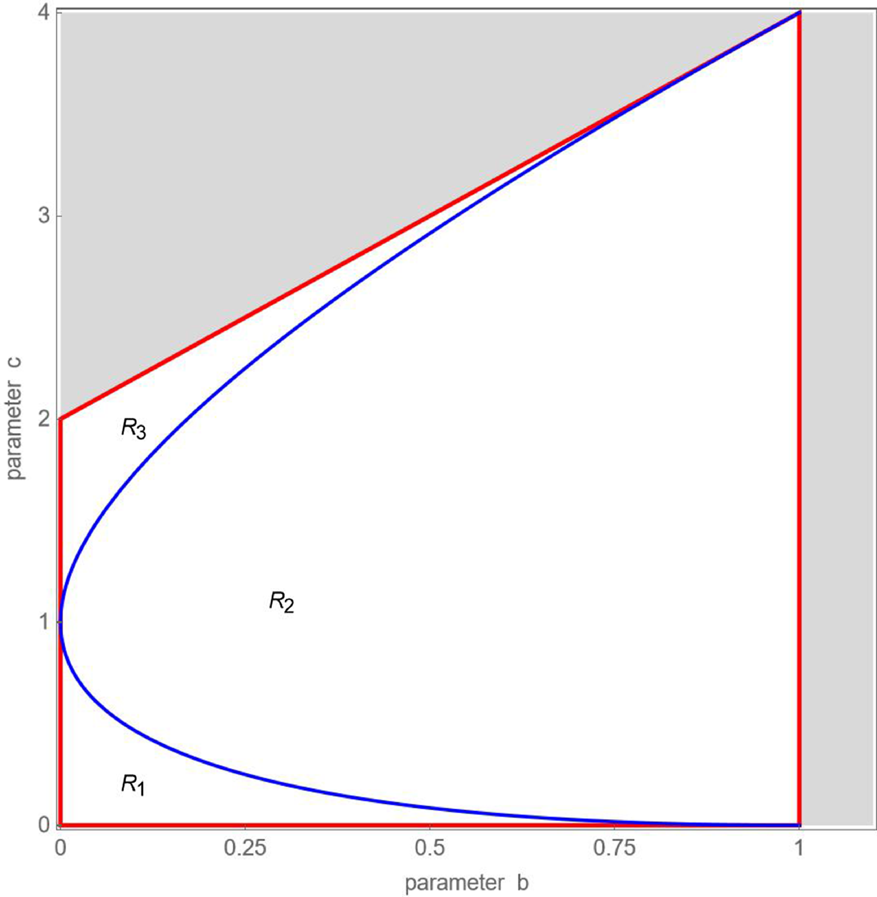
Figure 2 illustrates our analytical results for map $T_{R}$
. The black line in the top left panel shows the evolution of the stock price in the time domain, assuming that
$T_{R}$
. The black line in the top left panel shows the evolution of the stock price in the time domain, assuming that $b=0.1$
and
$b=0.1$
and $c=0.1$
; the red line depicts the stock market’s fundamental value. Since this parameter combination is located inside region
$c=0.1$
; the red line depicts the stock market’s fundamental value. Since this parameter combination is located inside region $R_{1}$
, the stock price monotonically approaches its fundamental value. The black line in the top right panel shows the stock price path for
$R_{1}$
, the stock price monotonically approaches its fundamental value. The black line in the top right panel shows the stock price path for $b=0.8$
and
$b=0.8$
and $c=0.2$
. As can be seen, the stock price exhibits dampened cyclical motion when the market impact of chartists and fundamentalists is located inside region
$c=0.2$
. As can be seen, the stock price exhibits dampened cyclical motion when the market impact of chartists and fundamentalists is located inside region $R_{2}$
. The black line in the bottom left panel visualizes a simulation of the stock price based on
$R_{2}$
. The black line in the bottom left panel visualizes a simulation of the stock price based on $b=0.1$
and
$b=0.1$
and $c=2.1$
. Since this parameter combination is located in region
$c=2.1$
. Since this parameter combination is located in region $R_{3}$
, we observe a zigzag adjustment path. Stock prices explode when parameters
$R_{3}$
, we observe a zigzag adjustment path. Stock prices explode when parameters $b$
and
$b$
and $c$
are located outside stability box
$c$
are located outside stability box $S$
. For
$S$
. For $b=0.1$
and
$b=0.1$
and $c=2.21$
, for instance, the amplitude of the zigzag path of the stock price increases, as reported in the bottom right panel.
$c=2.21$
, for instance, the amplitude of the zigzag path of the stock price increases, as reported in the bottom right panel.
Stock market dynamics for map $T_{R}$
. The black lines show the evolution of the stock price in the time domain; the red line marks fundamentalists’ correct perception of the stock market’s fundamental value. The four panels are based on
$T_{R}$
. The black lines show the evolution of the stock price in the time domain; the red line marks fundamentalists’ correct perception of the stock market’s fundamental value. The four panels are based on $b=0.1$
and
$b=0.1$
and $c=0.1$
,
$c=0.1$
, $b=0.8$
and
$b=0.8$
and $c=0.2$
,
$c=0.2$
, $b=0.1$
and
$b=0.1$
and $c=2.1$
and
$c=2.1$
and $b=0.1$
and
$b=0.1$
and $c=2.21$
, respectively. Initial conditions are given by
$c=2.21$
, respectively. Initial conditions are given by $x=0.05$
and
$x=0.05$
and $y=0$
.
$y=0$
.

We can thus conclude that—in the absence of animal spirits—the stock price will always converge to its fundamental value, provided that the trading behavior of chartists and fundamentalists does not become too aggressive. The latter means that parameters $b$
and
$b$
and $c$
must be located inside stability box
$c$
must be located inside stability box $S$
.
$S$
.
3.2. General properties of our stock market model
Before we characterize the behavior of our complete stock market model in detail, it is helpful to discuss a number of general properties of map $T_{C}$
.
$T_{C}$
.
Areas in $(x,y)$
-state space where maps
$(x,y)$
-state space where maps $T_{L}$
,
$T_{L}$
, $T_{U}$
and
$T_{U}$
and $T_{O}$
apply. In the area of map
$T_{O}$
apply. In the area of map $T_{L}$
, fundamentalists are optimistic. In the area of map
$T_{L}$
, fundamentalists are optimistic. In the area of map $T_{U}$
, fundamentalists are pessimistic. In the area of map
$T_{U}$
, fundamentalists are pessimistic. In the area of map $T_{O}$
, fundamentalists are neutral. Note that the real fixed point
$T_{O}$
, fundamentalists are neutral. Note that the real fixed point $P_{O}=(0,0)$
and the two virtual fixed points
$P_{O}=(0,0)$
and the two virtual fixed points $P_{L}=(d,d)$
and
$P_{L}=(d,d)$
and $P_{U}=(-d,-d)$
are located inside the area of map
$P_{U}=(-d,-d)$
are located inside the area of map $T_{O}$
.
$T_{O}$
.
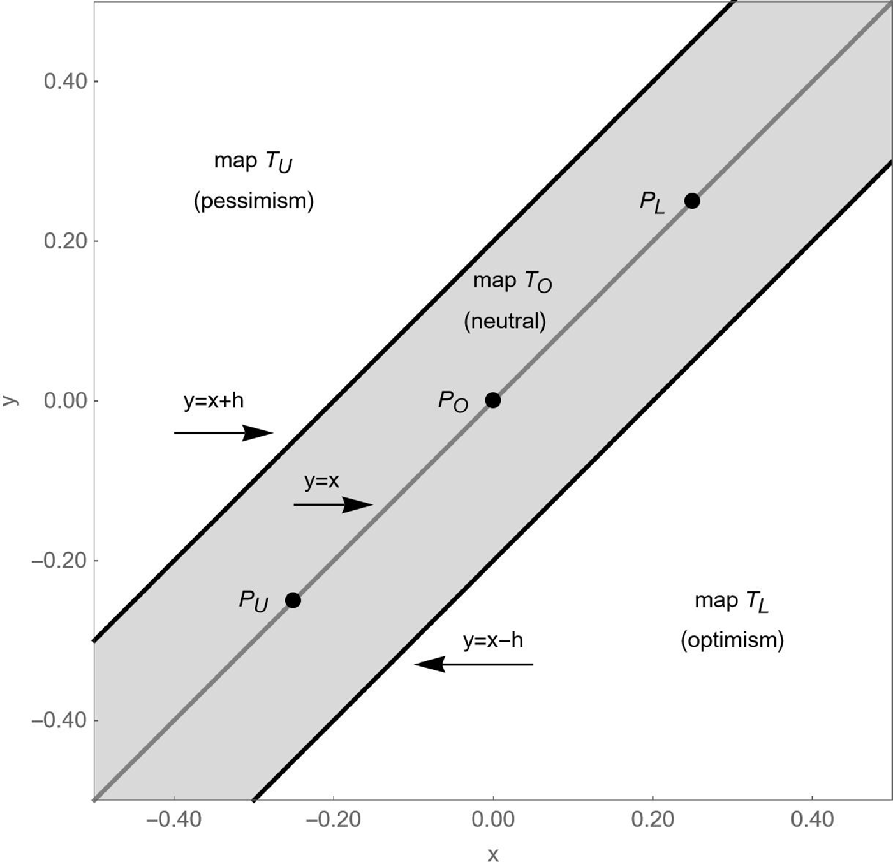
First, we can divide the $(x,y)$
-state space into three areas, each representing a different sentiment regime. See Figure 3 for an example. In the lower right part of the
$(x,y)$
-state space into three areas, each representing a different sentiment regime. See Figure 3 for an example. In the lower right part of the $(x,y)$
-state space, that is below the straight line
$(x,y)$
-state space, that is below the straight line $y=x-h$
, map
$y=x-h$
, map
 \begin{equation}T_{L}\colon \begin{cases} x'=\left(1+b-c\right)x-by+cd\\ y'=x \end{cases}\end{equation}
applies. In this area, fundamentalists optimistically believe in a high fundamental value since the stock price strongly increases. In the upper left part of the $(x,y)$
-state space, that is above the straight line
$(x,y)$
-state space, that is above the straight line $y=x+h$
, map
$y=x+h$
, map
 \begin{equation}T_{U}\colon \begin{cases} x'=\left(1+b-c\right)x-by-cd\\ y'=x \end{cases}\end{equation}
applies. In this area, fundamentalists pessimistically believe in a low fundamental value since the stock price strongly decreases. In the strip between these two straight lines, map
 \begin{equation}T_{O}\colon \begin{cases} x'=\left(1+b-c\right)x-by\\ y'=x \end{cases}\end{equation}
applies. In this area, stock prices are relatively stable. Hence, fundamentalists are neutral and believe in a normal fundamental value. As we will see, Figure 3 is key to understanding the functioning of our stock market model. Since the dynamics of our stock market model is governed by a map with two dimensions, knowledge about the current coordinates of $(x,y)=(x_{t},y_{t})=(x_{t},x_{t-1})=(P_{t}-F,P_{t-1}-F)$
allows us to immediately conclude which of the three maps
$(x,y)=(x_{t},y_{t})=(x_{t},x_{t-1})=(P_{t}-F,P_{t-1}-F)$
allows us to immediately conclude which of the three maps $T_{L}$
,
$T_{L}$
, $T_{U}$
and
$T_{U}$
and $T_{O}$
are responsible for determining the next stock price. Clearly, this is the beauty of two-dimensional maps; they give us a clear understanding of the system’s dynamics in the
$T_{O}$
are responsible for determining the next stock price. Clearly, this is the beauty of two-dimensional maps; they give us a clear understanding of the system’s dynamics in the $(x,y)$
-state space.
$(x,y)$
-state space.
Second, map $T_{O}$
is identical to map
$T_{O}$
is identical to map $T_{R}$
. Hence, the fixed point of map
$T_{R}$
. Hence, the fixed point of map $T_{O}$
, say
$T_{O}$
, say $P_{O}=(0,0)$
, has the same coordinates as the fixed point of map
$P_{O}=(0,0)$
, has the same coordinates as the fixed point of map $T_{R}$
. Of course, the fixed point
$T_{R}$
. Of course, the fixed point $P_{O}=(0,0)$
is also a fixed point of map
$P_{O}=(0,0)$
is also a fixed point of map $T_{C}$
. Importantly, however, the global stability results that we have established for the fixed point
$T_{C}$
. Importantly, however, the global stability results that we have established for the fixed point $P_{R}=(0,0)$
of map
$P_{R}=(0,0)$
of map $T_{R}$
may now only hold locally for the fixed point
$T_{R}$
may now only hold locally for the fixed point $P_{O}=(0,0)$
of map
$P_{O}=(0,0)$
of map $T_{C}$
. The following should be noted:
$T_{C}$
. The following should be noted:
-
• Proposition 1 in Appendix A states a sufficient condition for which the fixed point $P_{O}=(0,0)$
of map
$T_{C}$
is globally attracting. Figure 4, based on
$d=0.05$
and
$h=0.01$
, provides an example. For this parameter constellation, the fixed point
$P_{O}=(0,0)$
of map
$T_{C}$
is globally attracting for parameter combinations located inside (the green) region
$G$
(the sufficient condition requires that
$c\lt 0.2-0.25b$
). To establish globally stable stock markets, policymakers need to implement measures that force parameters
$b$
and
$c$
inside region
$G$
, e.g. by conducting transactions that counter those of chartists and fundamentalists.
$P_{O}=(0,0)$
of map
$T_{C}$
is globally attracting. Figure 4, based on
$d=0.05$
and
$h=0.01$
, provides an example. For this parameter constellation, the fixed point
$P_{O}=(0,0)$
of map
$T_{C}$
is globally attracting for parameter combinations located inside (the green) region
$G$
(the sufficient condition requires that
$c\lt 0.2-0.25b$
). To establish globally stable stock markets, policymakers need to implement measures that force parameters
$b$
and
$c$
inside region
$G$
, e.g. by conducting transactions that counter those of chartists and fundamentalists. -
• Proposition 2 in Appendix B states a sufficient condition for which the fixed point
$P_{O}=(0,0)$
of map
$T_{C}$
coexists with one or more cyclical attractors. In Figure 4, this is the case for
$c\gt 1/3$
. Proposition 2 furthermore characterizes the basin of attraction of the fixed point
$P_{O}=(0,0)$
of map
$T_{C}$
in the presence of coexisting attractors. To be more precise, we can conclude from Proposition 2 that the basin of attraction of the fixed point
$P_{O}=(0,0)$
of map
$T_{C}$
belongs to a quadrilateral region
$Q$
with vertices
$(x_{L}^{*},y_{L}^{*})$
,
$(x_{U}^{*},y_{U}^{*})$
,
$(-x_{L}^{*},-y_{L}^{*})$
and
$(-x_{U}^{*},-y_{U}^{*})$
, where
$(x_{L}^{*},y_{L}^{*})=(h(1+b)/c,x_{L}^{*}-h)$
and
$(x_{U}^{*},y_{U}^{*})=(h(1-b)/c,$
$x_{U}^{*}+h)$
. Let us return to Figure 4. For parameter combinations located inside (the blue) region
$E$
, the basin of attraction of the fixed point
$P_{O}=(0,0)$
of map
$T_{C}$
is equal to region
$Q$
. For parameter combinations located inside one of the two (yellow) regions
$U$
, the basin of attraction of the fixed point
$P_{O}=(0,0)$
of map
$T_{C}$
is smaller than region
$Q$
. For parameter combinations located inside (the orange) region
$A$
, the basin of attraction of the fixed point
$P_{O}=(0,0)$
of map
$T_{C}$
may be smaller or larger than region
$Q$
. As long as the stock price remains inside the basin of attraction of the fixed point
$P_{O}=(0,0)$
of map
$T_{C}$
, its trajectory will describe a cyclical, monotonic or alternating adjustment path towards its fundamental value, depending on whether parameters
$b$
and
$c$
are located inside regions
$R_{1}$
,
$R_{2}$
and
$R_{3}$
, respectively. The dynamics we have witnessed in Figure 2 for map
$T_{R}$
thus also holds for map
$T_{C}$
, assuming that the stock price remains in the vicinity of its fixed point
$P_{O}=(0,0)$
.


Sections 3.3 to 3.5 discuss the economic implications of these results in more detail.
Properties of map $T_{C}$
in the
$T_{C}$
in the $(b,c)$
-parameter plane. Green region
$(b,c)$
-parameter plane. Green region $G$
: the real fixed point is globally attracting. Blue region
$G$
: the real fixed point is globally attracting. Blue region $E$
: the basin of attraction of the real fixed point is equal to the quadrilateral region
$E$
: the basin of attraction of the real fixed point is equal to the quadrilateral region $Q$
. Yellow regions
$Q$
. Yellow regions $U$
: the basin of attraction of the real fixed point is smaller than the quadrilateral region
$U$
: the basin of attraction of the real fixed point is smaller than the quadrilateral region $Q$
. Orange region
$Q$
. Orange region $A$
: the basin of attraction of the real fixed point may be smaller or larger than the quadrilateral region
$A$
: the basin of attraction of the real fixed point may be smaller or larger than the quadrilateral region $Q$
. White region
$Q$
. White region $C$
: coexistence of chaotic and divergent dynamics. Gray region
$C$
: coexistence of chaotic and divergent dynamics. Gray region $D$
: divergent dynamics. Remaining parameters:
$D$
: divergent dynamics. Remaining parameters: $d=0.05$
and
$d=0.05$
and $h=0.01$
.
$h=0.01$
.

Third, the fixed points of maps $T_{L}$
and
$T_{L}$
and $T_{U}$
are given by
$T_{U}$
are given by $P_{L}=(d,d)$
and
$P_{L}=(d,d)$
and $P_{U}=(-d,-d)$
, respectively. While the fixed point
$P_{U}=(-d,-d)$
, respectively. While the fixed point $P_{L}=(d,d)$
represents an overvalued stock market, the fixed point
$P_{L}=(d,d)$
represents an overvalued stock market, the fixed point $P_{U}=(-d,-d)$
signifies an undervalued stock market. Since these fixed points are located on the diagonal of the
$P_{U}=(-d,-d)$
signifies an undervalued stock market. Since these fixed points are located on the diagonal of the $(x,y)$
-state space, as evidenced in Figure 3, they do not belong to the area where their maps apply. For this reason, the fixed points
$(x,y)$
-state space, as evidenced in Figure 3, they do not belong to the area where their maps apply. For this reason, the fixed points $P_{L}=(d,d)$
and
$P_{L}=(d,d)$
and $P_{U}=(-d,-d)$
are virtual fixed point for map
$P_{U}=(-d,-d)$
are virtual fixed point for map $T_{C}$
. Put differently, map
$T_{C}$
. Put differently, map $T_{C}$
has three fixed points, which we will call the optimistic virtual fixed point
$T_{C}$
has three fixed points, which we will call the optimistic virtual fixed point $P_{L}=(d,d)$
, the real fixed point
$P_{L}=(d,d)$
, the real fixed point $P_{O}=(0,0)$
, and the pessimistic virtual fixed point
$P_{O}=(0,0)$
, and the pessimistic virtual fixed point $P_{U}=(-d,-d)$
.
$P_{U}=(-d,-d)$
.
Fourth, virtual fixed points may have a significant impact on stock market dynamics, as revealed by the following thought experiment. Recall first that maps $T_{L}$
and
$T_{L}$
and $T_{U}$
have the same Jacobian matrix and thus the same eigenvalues as map
$T_{U}$
have the same Jacobian matrix and thus the same eigenvalues as map $T_{O}$
, implying that their fixed points share the same stability properties. Let us assume, for simplicity, that parameters
$T_{O}$
, implying that their fixed points share the same stability properties. Let us assume, for simplicity, that parameters $b$
and
$b$
and $c$
are located inside region
$c$
are located inside region $R_{1}$
. As a result, the stock price will converge monotonically to a virtual fixed point as long as its trajectory remains inside the area where its map applies. Suppose that the stock price monotonically approaches the optimistic virtual fixed point. Since the stock price change associated with a convergence to this fixed point decreases over time, the stock price will eventually leave this area. This causes a regime change, which may initially result in a movement towards the real fixed point. Suppose that this regime change is associated with a sharp movement towards the real fixed point, a movement that exceeds parameter
$R_{1}$
. As a result, the stock price will converge monotonically to a virtual fixed point as long as its trajectory remains inside the area where its map applies. Suppose that the stock price monotonically approaches the optimistic virtual fixed point. Since the stock price change associated with a convergence to this fixed point decreases over time, the stock price will eventually leave this area. This causes a regime change, which may initially result in a movement towards the real fixed point. Suppose that this regime change is associated with a sharp movement towards the real fixed point, a movement that exceeds parameter $h$
. Then there is another regime change, and the stock price moves monotonically toward the pessimistic virtual fixed point, albeit only for a few time steps, as the rate of adjustment automatically slows down over time. Importantly, the virtual fixed points of map
$h$
. Then there is another regime change, and the stock price moves monotonically toward the pessimistic virtual fixed point, albeit only for a few time steps, as the rate of adjustment automatically slows down over time. Importantly, the virtual fixed points of map $T_{C}$
are temporarily attracting but any convergence towards them is eventually self-defeating. As long as the stock price does not get stuck in the basin of attraction of the real fixed point, the existence of virtual fixed points provides the stage for sentiment-driven boom-bust stock market dynamics. We can observe this cycle-generating mechanism in regions
$T_{C}$
are temporarily attracting but any convergence towards them is eventually self-defeating. As long as the stock price does not get stuck in the basin of attraction of the real fixed point, the existence of virtual fixed points provides the stage for sentiment-driven boom-bust stock market dynamics. We can observe this cycle-generating mechanism in regions $R_{1}$
,
$R_{1}$
, $R_{2}$
and
$R_{2}$
and $R_{3}$
, as made clear in Sections 3.3 to 3.5.
$R_{3}$
, as made clear in Sections 3.3 to 3.5.
Fifth, numerical evidence suggests that stability box $S$
is almost completely filled with families of different types of stock price cycles. The two-dimensional bifurcation diagram depicted in Figure 5 is a first example. Parameters
$S$
is almost completely filled with families of different types of stock price cycles. The two-dimensional bifurcation diagram depicted in Figure 5 is a first example. Parameters $b$
and
$b$
and $c$
are varied as in Figure 1, while the remaining parameters are set to
$c$
are varied as in Figure 1, while the remaining parameters are set to $d=0.05$
and
$d=0.05$
and $h=0.01$
. The initial conditions are given by
$h=0.01$
. The initial conditions are given by $x=0.025$
and
$x=0.025$
and $y=0$
.Footnote 8 Different colors indicate numerically detected stock price cycles with different periods. For instance, the large red, blue, green and yellow areas in the left part of the two-dimensional bifurcation diagram represent parameter combinations that lead to period-4, period-6, period-8 and period-10 stock price cycles, respectively. Moreover, the (smaller) cyan, pink and brown areas in the middle part of the two-dimensional bifurcation diagram reflect parameter combinations that give rise to period-3, period-5 and period-7 stock price cycles, respectively. Parameter combinations that yield cycles with a lag larger than
$y=0$
.Footnote 8 Different colors indicate numerically detected stock price cycles with different periods. For instance, the large red, blue, green and yellow areas in the left part of the two-dimensional bifurcation diagram represent parameter combinations that lead to period-4, period-6, period-8 and period-10 stock price cycles, respectively. Moreover, the (smaller) cyan, pink and brown areas in the middle part of the two-dimensional bifurcation diagram reflect parameter combinations that give rise to period-3, period-5 and period-7 stock price cycles, respectively. Parameter combinations that yield cycles with a lag larger than $n=42$
are marked purple. Black areas stand for parameter combinations for which the stock price convergences to the real fixed point. White areas mark parameter combinations that yield chaotic stock price dynamics. Gray areas reflect parameter combinations that are associated with divergent dynamics. Qualitatively similar images are obtained for different values of parameters
$n=42$
are marked purple. Black areas stand for parameter combinations for which the stock price convergences to the real fixed point. White areas mark parameter combinations that yield chaotic stock price dynamics. Gray areas reflect parameter combinations that are associated with divergent dynamics. Qualitatively similar images are obtained for different values of parameters $d$
and
$d$
and $h$
, provided that
$h$
, provided that $d\gt h\gt 0$
.
$d\gt h\gt 0$
.
Two-dimensional bifurcation diagram in the $(b,c)$
-parameter plane for map
$(b,c)$
-parameter plane for map $T_{C}$
. Differently colored areas mark periodicity regions of different cycles (areas that produce cycles with a period larger than
$T_{C}$
. Differently colored areas mark periodicity regions of different cycles (areas that produce cycles with a period larger than $n=42$
are marked purple). Black areas mark parameter combinations that result in a convergence to the real fixed point. White areas mark parameter combinations that lead to chaotic dynamics. Gray areas mark parameter combinations that yield divergent dynamics. Numerical observations rely on initial conditions
$n=42$
are marked purple). Black areas mark parameter combinations that result in a convergence to the real fixed point. White areas mark parameter combinations that lead to chaotic dynamics. Gray areas mark parameter combinations that yield divergent dynamics. Numerical observations rely on initial conditions $x=0.025$
and
$x=0.025$
and $y=0$
. Remaining parameters:
$y=0$
. Remaining parameters: $d=0.05$
and
$d=0.05$
and $h=0.01$
.
$h=0.01$
.

Sixth, map $T_{C}$
is symmetric with respect to the real fixed point
$T_{C}$
is symmetric with respect to the real fixed point $P_{O}=(0,0)$
. Since
$P_{O}=(0,0)$
. Since $T_{O}(-x,-y)=-T_{O}(x,y)$
and
$T_{O}(-x,-y)=-T_{O}(x,y)$
and $T_{U}(-x,-y)=-T_{L}(x,y)$
, it follows that the trajectory starting at point
$T_{U}(-x,-y)=-T_{L}(x,y)$
, it follows that the trajectory starting at point $(-x_{0},-y_{0})$
is symmetric with respect to the real fixed point
$(-x_{0},-y_{0})$
is symmetric with respect to the real fixed point $P_{O}=(0,0)$
to the trajectory of point
$P_{O}=(0,0)$
to the trajectory of point $(x_{0},y_{0})$
. This means that any invariant set
$(x_{0},y_{0})$
. This means that any invariant set $A$
of map
$A$
of map $T$
is symmetric with respect to the real fixed point
$T$
is symmetric with respect to the real fixed point $P_{O}=(0,0)$
or an invariant set
$P_{O}=(0,0)$
or an invariant set $A'$
exists that is symmetric to
$A'$
exists that is symmetric to $A$
with respect to the real fixed point
$A$
with respect to the real fixed point $P_{O}=(0,0)$
. Hence, any odd-period cycle has a symmetric companion odd-period cycle. Since Figure 5 reports multiple instances of odd-period cycles, this is a first indication that our stock market model may give rise to coexisting cyclical attractors. In Sections 3.3 to 3.5, we will see that there are further forms of coexisting periodic attractors, e.g. odd-period cycles may coexist with one or more even-period cycles. From the next remark, it follows that all existing cycles in stability box
$P_{O}=(0,0)$
. Hence, any odd-period cycle has a symmetric companion odd-period cycle. Since Figure 5 reports multiple instances of odd-period cycles, this is a first indication that our stock market model may give rise to coexisting cyclical attractors. In Sections 3.3 to 3.5, we will see that there are further forms of coexisting periodic attractors, e.g. odd-period cycles may coexist with one or more even-period cycles. From the next remark, it follows that all existing cycles in stability box $S$
are attracting.
$S$
are attracting.
Seventh, the fact that maps $T_{L}$
,
$T_{L}$
, $T_{O}$
and
$T_{O}$
and $T_{U}$
have the same Jacobian matrix
$T_{U}$
have the same Jacobian matrix $J$
leads to an important property with respect to the stability or instability of all possible existing cycles of map
$J$
leads to an important property with respect to the stability or instability of all possible existing cycles of map $T_{C}$
. In fact, a cycle of period
$T_{C}$
. In fact, a cycle of period $n$
is a fixed point of the
$n$
is a fixed point of the $n$
-th iterate of map
$n$
-th iterate of map $T_{C}^{n}$
. Its stability is therefore determined by the eigenvalues of matrix
$T_{C}^{n}$
. Its stability is therefore determined by the eigenvalues of matrix $J^{n}$
, which in turn are given by
$J^{n}$
, which in turn are given by $\lambda _{1}^{n}$
and
$\lambda _{1}^{n}$
and $\lambda _{2}^{n}$
. In particular, for all combinations of parameters
$\lambda _{2}^{n}$
. In particular, for all combinations of parameters $b$
and
$b$
and $c$
located inside stability box
$c$
located inside stability box $S$
, map
$S$
, map $T_{C}$
cannot have unstable cycles. Since this also rules out the existence of divergent dynamics for all combinations of parameters
$T_{C}$
cannot have unstable cycles. Since this also rules out the existence of divergent dynamics for all combinations of parameters $b$
and
$b$
and $c$
located inside stability box
$c$
located inside stability box $S$
, we can still define that parameter region as a stability region for map
$S$
, we can still define that parameter region as a stability region for map $T_{C}$
. For all combinations of parameters
$T_{C}$
. For all combinations of parameters $b$
and
$b$
and $c$
not located inside stability box
$c$
not located inside stability box $S$
, map
$S$
, map $T_{C}$
cannot have stable cycles.
$T_{C}$
cannot have stable cycles.
Eighth, Figure 5 reports numerical evidence for the existence of attracting cycles. In a mathematical companion paper, Gardini et al. (Reference Gardini, Radi, Schmitt, Sushko and Westerhoff2023a) explain how to derive analytical expressions for the bifurcation boundaries of different types of families of cycles. While they study a different stock market model, their mathematical techniques also apply to our map. Based on their insights, Figure 6 exemplarily portrays analytically determined bifurcation boundaries of two qualitatively different locally stable period-6 stock price cycles in the $(b,c)$
-parameter plane for map
$(b,c)$
-parameter plane for map $T_{C}$
. Parameters
$T_{C}$
. Parameters $b$
and
$b$
and $c$
are varied as in Figures 1, 4 and 5, while the remaining parameters are set to
$c$
are varied as in Figures 1, 4 and 5, while the remaining parameters are set to $d=0.05$
and
$d=0.05$
and $h=0.01$
. The area between the two cyan curves marks the existence region of a period-6 stock price cycle that involves all three branches of map
$h=0.01$
. The area between the two cyan curves marks the existence region of a period-6 stock price cycle that involves all three branches of map $T_{C}$
. Note that the existence region of this period-6 stock price cycle covers parts of regions
$T_{C}$
. Note that the existence region of this period-6 stock price cycle covers parts of regions $R_{1}$
,
$R_{1}$
, $R_{2}$
and
$R_{2}$
and $R_{3}$
. Clearly, this proves that our stock market model is able to produce endogenous stock market dynamics in regions
$R_{3}$
. Clearly, this proves that our stock market model is able to produce endogenous stock market dynamics in regions $R_{1}$
,
$R_{1}$
, $R_{2}$
and
$R_{2}$
and $R_{3}$
. The area between the two purple curves marks the existence region of a period-6 stock price cycle that only involves two of the three branches of map
$R_{3}$
. The area between the two purple curves marks the existence region of a period-6 stock price cycle that only involves two of the three branches of map $T_{C}$
. Note that the existence region of this cycle is entirely located inside region
$T_{C}$
. Note that the existence region of this cycle is entirely located inside region $R_{2}$
. Obviously, both period-6 stock price cycles coexist in the area between the two cyan and the two purple curves—next to the locally stable real fixed point. We will return to this interesting scenario in Section 3.4. As it turns out, the analytically determined area between the two cyan curves or the two purple curves in Figure 6 nicely overlaps with the numerically identified existence region of period-6 stock price cycles reported in Figure 5. Of course, it is not clear from Figure 5 that we are dealing with two qualitatively different period-6 stock price cycles. Moreover, the image of the two-dimensional bifurcation diagram presented in Figure 5 depends on the initial conditions; other initial conditions may result in different images. In Appendix C, we explicitly derive the analytical bifurcation boundaries reported in Figure 6. We recall that it is possible to determine the analytical bifurcation boundaries for other families of cycles, too.
$R_{2}$
. Obviously, both period-6 stock price cycles coexist in the area between the two cyan and the two purple curves—next to the locally stable real fixed point. We will return to this interesting scenario in Section 3.4. As it turns out, the analytically determined area between the two cyan curves or the two purple curves in Figure 6 nicely overlaps with the numerically identified existence region of period-6 stock price cycles reported in Figure 5. Of course, it is not clear from Figure 5 that we are dealing with two qualitatively different period-6 stock price cycles. Moreover, the image of the two-dimensional bifurcation diagram presented in Figure 5 depends on the initial conditions; other initial conditions may result in different images. In Appendix C, we explicitly derive the analytical bifurcation boundaries reported in Figure 6. We recall that it is possible to determine the analytical bifurcation boundaries for other families of cycles, too.
Analytically determined bifurcation boundaries of two qualitatively different locally stable period-6 cycles in the $(b,c)$
-parameter plane for map
$(b,c)$
-parameter plane for map $T_{C}$
. The area between the two cyan curves marks the existence region of a period-6 cycle, covering parts of regions
$T_{C}$
. The area between the two cyan curves marks the existence region of a period-6 cycle, covering parts of regions $R_{1}$
,
$R_{1}$
, $R_{2}$
and
$R_{2}$
and $R_{3}$
. The area between the two purple curves marks the existence region of another period-6 cycle, covering part of region
$R_{3}$
. The area between the two purple curves marks the existence region of another period-6 cycle, covering part of region $R_{2}$
. Both period-6 cycles coexist in the area between the two cyan and the two purple curves. Remaining parameters:
$R_{2}$
. Both period-6 cycles coexist in the area between the two cyan and the two purple curves. Remaining parameters: $d=0.05$
and
$d=0.05$
and $h=0.01$
.
$h=0.01$
.

Ninth, the white triangle-like region in the two-dimensional bifurcation diagram depicted in Figure 5 represents $(b,c)$
-parameter combinations for which we found chaotic stock price dynamics. In the absence of animal spirits, these parameter combinations would yield divergent stock price dynamics. In the presence of animal spirits, the stock price may exhibit at least bounded dynamics. In this sense, animal spirits can also have a stabilizing impact on stock market dynamics. Since the real fixed point, as well as any other existing cycle of our stock market model, is of course not stable in this parameter region, the chaotic attractor does not coexist with an attracting real fixed point or cycle. However, the dynamics in this parameter domain may also be divergent: stock prices explode when initial conditions exit the basin of attraction of the chaotic attractor. We discuss this issue in more detail in Section 4.1. One further comment is in order. The two-dimensional bifurcation diagram depicted in Figure 5 is the outcome of a simulation exercise. In Appendix D, we analytically derive the existence region of chaotic stock market dynamics. The white region
$(b,c)$
-parameter combinations for which we found chaotic stock price dynamics. In the absence of animal spirits, these parameter combinations would yield divergent stock price dynamics. In the presence of animal spirits, the stock price may exhibit at least bounded dynamics. In this sense, animal spirits can also have a stabilizing impact on stock market dynamics. Since the real fixed point, as well as any other existing cycle of our stock market model, is of course not stable in this parameter region, the chaotic attractor does not coexist with an attracting real fixed point or cycle. However, the dynamics in this parameter domain may also be divergent: stock prices explode when initial conditions exit the basin of attraction of the chaotic attractor. We discuss this issue in more detail in Section 4.1. One further comment is in order. The two-dimensional bifurcation diagram depicted in Figure 5 is the outcome of a simulation exercise. In Appendix D, we analytically derive the existence region of chaotic stock market dynamics. The white region $C$
in Figure 4 visualizes the analytically determined existence region of chaotic stock market dynamics for
$C$
in Figure 4 visualizes the analytically determined existence region of chaotic stock market dynamics for $d=0.05$
and
$d=0.05$
and $h=0.01$
.
$h=0.01$
.
Tenth, we also show in Appendix D that the gray area in the two-dimensional bifurcation diagram depicted in Figure 5 represents $(b,c)$
-parameter combinations that must necessarily result in divergent dynamics. While Figure 5 is based on numerical results, the gray region in Figure 4, which again reflects divergent dynamics, visualizes our analytical results.
$(b,c)$
-parameter combinations that must necessarily result in divergent dynamics. While Figure 5 is based on numerical results, the gray region in Figure 4, which again reflects divergent dynamics, visualizes our analytical results.
Example of stock price dynamics in region $R_{1}$
. Left: the blue line shows the evolution of a period-8 stock price cycle in the time domain. The red solid and dashed lines mark fundamentalists’ correct and biased perception of the stock market’s fundamental value, respectively. Right: the connected blue disks depict the evolution of a period-8 stock price cycle in
$R_{1}$
. Left: the blue line shows the evolution of a period-8 stock price cycle in the time domain. The red solid and dashed lines mark fundamentalists’ correct and biased perception of the stock market’s fundamental value, respectively. Right: the connected blue disks depict the evolution of a period-8 stock price cycle in $(x,y)$
-state space; the red disk and the two red circles indicate the positions of the real fixed point and the two virtual fixed points. The two black dashed lines and the two black dotted lines represent the discontinuity lines
$(x,y)$
-state space; the red disk and the two red circles indicate the positions of the real fixed point and the two virtual fixed points. The two black dashed lines and the two black dotted lines represent the discontinuity lines $y=x+h$
and
$y=x+h$
and $y=x-h$
and their rank-1 preimages via map
$y=x-h$
and their rank-1 preimages via map $T_{O}^{-1}$
, respectively. The four red segments of the quadrilateral region
$T_{O}^{-1}$
, respectively. The four red segments of the quadrilateral region $Q$
bound the analytically determined basin of attraction of the real fixed point. The light blue and light red areas mark the numerically detected basins of attraction of the period-8 cycle and of the real fixed point, respectively. Parameter setting:
$Q$
bound the analytically determined basin of attraction of the real fixed point. The light blue and light red areas mark the numerically detected basins of attraction of the period-8 cycle and of the real fixed point, respectively. Parameter setting: $b=0.05$
,
$b=0.05$
, $c=0.5$
,
$c=0.5$
, $d=0.05$
and
$d=0.05$
and $h=0.01$
.
$h=0.01$
.

Eleventh, the black area in the two-dimensional bifurcation diagram depicted in Figure 5 represents $(b,c)$
-parameter combinations for which the stock price approaches its real fixed point in our numerical investigation (with the considered initial condition). In that region, there are still values of the parameters for which the attracting fixed point coexists with one or more attracting cycles. Region
$(b,c)$
-parameter combinations for which the stock price approaches its real fixed point in our numerical investigation (with the considered initial condition). In that region, there are still values of the parameters for which the attracting fixed point coexists with one or more attracting cycles. Region $G$
in Figure 4 portrays analytically identified parameter combinations for which the real fixed point is the only attractor, that is, it is globally attracting.
$G$
in Figure 4 portrays analytically identified parameter combinations for which the real fixed point is the only attractor, that is, it is globally attracting.
Once again, we stress that the aforementioned differences between the trivial dynamics of map $T_{R}$
and the more intriguing dynamics of map
$T_{R}$
and the more intriguing dynamics of map $T_{C}$
are entirely due to fundamentalists’ animal spirits, that is their time-varying perception of the stock market’s fundamental value. In the following, we explore the dynamics of our stock market model in regions
$T_{C}$
are entirely due to fundamentalists’ animal spirits, that is their time-varying perception of the stock market’s fundamental value. In the following, we explore the dynamics of our stock market model in regions $R_{1}$
,
$R_{1}$
, $R_{2}$
and
$R_{2}$
and $R_{3}$
.
$R_{3}$
.
3.3. Stock market dynamics in region
$\boldsymbol{R}_{\boldsymbol{1}}$

Figure 7, based on $b=0.05$
,
$b=0.05$
, $c=0.5$
,
$c=0.5$
, $d=0.05$
and
$d=0.05$
and $h=0.01$
, presents an example of the dynamics of our stock market model in region
$h=0.01$
, presents an example of the dynamics of our stock market model in region $\boldsymbol{R}_{\boldsymbol{1}}$
. For this parameter setting, the real fixed point coexists with a period-8 stock price cycle. In the left panel, we depict the evolution of the period-8 stock price cycle (blue line) and fundamentalists’ correct and biased perceptions of the stock market’s fundamental value (red solid and dashed lines) in the time domain. The connected blue disks depicted in the right panel represent the evolution of the period-8 stock price cycle in
$\boldsymbol{R}_{\boldsymbol{1}}$
. For this parameter setting, the real fixed point coexists with a period-8 stock price cycle. In the left panel, we depict the evolution of the period-8 stock price cycle (blue line) and fundamentalists’ correct and biased perceptions of the stock market’s fundamental value (red solid and dashed lines) in the time domain. The connected blue disks depicted in the right panel represent the evolution of the period-8 stock price cycle in $(x,y)$
-state space. The red disk and the two red circles reflect the positions of the real fixed point and the two virtual fixed points. The light blue and light red areas indicate the numerically identified basins of attraction of the period-8 stock price cycle and of the real fixed point, respectively. The two black dashed lines and the two black dotted lines represent the discontinuity lines
$(x,y)$
-state space. The red disk and the two red circles reflect the positions of the real fixed point and the two virtual fixed points. The light blue and light red areas indicate the numerically identified basins of attraction of the period-8 stock price cycle and of the real fixed point, respectively. The two black dashed lines and the two black dotted lines represent the discontinuity lines $y=x+h$
and
$y=x+h$
and $y=x-h$
and their rank-1 preimages via map
$y=x-h$
and their rank-1 preimages via map $T_{O}^{-1}$
, respectively. The four red segments of the quadrilateral region
$T_{O}^{-1}$
, respectively. The four red segments of the quadrilateral region $Q$
indicate the analytically determined basin of attraction of the real fixed point.
$Q$
indicate the analytically determined basin of attraction of the real fixed point.
In the following, we explain the functioning of our stock market model in region $R_{1}$
.Footnote 9 For the initial conditions located in the light blue area, the stock price encircles its fundamental value in the form of a period-8 cycle. The rounded time series recordings of the period-8 stock price cycle read
$R_{1}$
.Footnote 9 For the initial conditions located in the light blue area, the stock price encircles its fundamental value in the form of a period-8 cycle. The rounded time series recordings of the period-8 stock price cycle read $\{-0.0220$
,
$\{-0.0220$
, $0.0150$
,
$0.0150$
, $0.0334$
,
$0.0334$
, $0.0432$
,
$0.0432$
, $0.0220$
,
$0.0220$
, $-0.0150$
,
$-0.0150$
, $-0.0334$
,
$-0.0334$
, $-0.0432\}$
, while the rounded state-space coordinates of the period-8 stock price cycle are equal to
$-0.0432\}$
, while the rounded state-space coordinates of the period-8 stock price cycle are equal to $\{(0.0150$
,
$\{(0.0150$
, $-0.0220$
), (
$-0.0220$
), ( $0.0334$
,
$0.0334$
, $0.0150$
), (
$0.0150$
), ( $0.0432$
,
$0.0432$
, $0.0334$
), (
$0.0334$
), ( $0.0220$
,
$0.0220$
, $0.0432$
), (
$0.0432$
), ( $-0.0150$
,
$-0.0150$
, $0.0220$
), (
$0.0220$
), ( $-0.0334$
,
$-0.0334$
, $-0.0150$
), (
$-0.0150$
), ( $-0.0432$
,
$-0.0432$
, $-0.0334$
), (
$-0.0334$
), ( $-0.0220$
,
$-0.0220$
, $-0.0432)\}$
. For completeness, we recall that the fundamental value of the stock price is equal to
$-0.0432)\}$
. For completeness, we recall that the fundamental value of the stock price is equal to $F=0$
. In addition, fundamentalists either believe in the normal fundamental value
$F=0$
. In addition, fundamentalists either believe in the normal fundamental value $F^{n}=0$
, the high fundamental value
$F^{n}=0$
, the high fundamental value $F^{o}=0.05$
or the low fundamental value
$F^{o}=0.05$
or the low fundamental value $F^{p}=-0.05$
. Hence, the coordinates of the real fixed point are given by
$F^{p}=-0.05$
. Hence, the coordinates of the real fixed point are given by $P_{O}=(0,0)$
, while those of the optimistic and pessimistic virtual fixed points are equal to
$P_{O}=(0,0)$
, while those of the optimistic and pessimistic virtual fixed points are equal to $P_{L}=(0.05,0.05)$
and
$P_{L}=(0.05,0.05)$
and $P_{U}=(-0.05,-0.05)$
, respectively.
$P_{U}=(-0.05,-0.05)$
, respectively.
As a starting point, we use the stock price increases from $-0.0220$
to
$-0.0220$
to $0.0150$
. In state space, this stock price increase is represented by the point
$0.0150$
. In state space, this stock price increase is represented by the point $(0.0150,-0.0220)$
. Due to the significant increase in the stock price, fundamentalists are optimistic and believe in the high fundamental value
$(0.0150,-0.0220)$
. Due to the significant increase in the stock price, fundamentalists are optimistic and believe in the high fundamental value $F^{o}$
. Since chartists also receive a buying signal, their joint orders drive the stock price upwards. Technically speaking, the stock price increases monotonically for two further time steps, from
$F^{o}$
. Since chartists also receive a buying signal, their joint orders drive the stock price upwards. Technically speaking, the stock price increases monotonically for two further time steps, from $0.0150$
to
$0.0150$
to $0.0344$
and from
$0.0344$
and from $0.0344$
to
$0.0344$
to $0.0432$
, straight toward its optimistic virtual fixed point
$0.0432$
, straight toward its optimistic virtual fixed point $P_{L}$
. In state space, this movement involves points
$P_{L}$
. In state space, this movement involves points $(0.0150,-0.0220)$
, (
$(0.0150,-0.0220)$
, ( $0.0344,0.0150$
) and (
$0.0344,0.0150$
) and ( $0.0432,0.0344$
). Note that the last increase in the stock price falls short of the optimistic sentiment threshold
$0.0432,0.0344$
). Note that the last increase in the stock price falls short of the optimistic sentiment threshold $h=0.01$
. Economically speaking, this means that fundamentalists come to their senses and correct their mistakes, that is they become neutral instead of optimistic and therefore believe in the correct normal fundamental value
$h=0.01$
. Economically speaking, this means that fundamentalists come to their senses and correct their mistakes, that is they become neutral instead of optimistic and therefore believe in the correct normal fundamental value $F^{n}$
.
$F^{n}$
.
Since the stock market appears overvalued to them, fundamentalists place sell orders. These sell orders dominate chartists’ buy orders, as the stock price increases only weakly. Hence, the market maker decreases the stock price. In technical terms, the stock price is now attracted by the real fixed point $P_{O}$
. After one time step, the stock price drops to
$P_{O}$
. After one time step, the stock price drops to $0.0220$
. This is presented by point (
$0.0220$
. This is presented by point ( $0.0220,0.0432$
). Note that this drop in the stock price exceeds the pessimistic sentiment threshold
$0.0220,0.0432$
). Note that this drop in the stock price exceeds the pessimistic sentiment threshold $h=-0.01$
, which is why fundamentalists become pessimistic. From this moment on, they believe in the low fundamental value
$h=-0.01$
, which is why fundamentalists become pessimistic. From this moment on, they believe in the low fundamental value $F^{p}$
.
$F^{p}$
.
As a result, fundamentalists regard the stock market as significantly overvalued. Due to the downward trend of the stock market, chartists receive a selling signal, too. Consequently, the stock price converges monotonically to the pessimistic virtual fixed point $P_{U}$
. After two further stock price drops, from
$P_{U}$
. After two further stock price drops, from $0.0220$
to
$0.0220$
to $-0.0150$
and from
$-0.0150$
and from $-0.0150$
to
$-0.0150$
to $-0.0334$
, the stock market falls once again and the stock price drops to
$-0.0334$
, the stock market falls once again and the stock price drops to $-0.0432$
. This downward movement involves points (
$-0.0432$
. This downward movement involves points ( $-0.0150$
, 0.0220), (
$-0.0150$
, 0.0220), ( $-0.0334$
,
$-0.0334$
, $-0.0150$
) and (
$-0.0150$
) and ( $-0.0432$
,
$-0.0432$
, $-0.0334$
). Since the last drop in the stock price is lower than
$-0.0334$
). Since the last drop in the stock price is lower than $h=-0.01$
, fundamentalists recover from their pessimism. Once again, they come to their senses and correct their mistakes. Now their neutral attitude leads them to believe again in the correct normal fundamental value
$h=-0.01$
, fundamentalists recover from their pessimism. Once again, they come to their senses and correct their mistakes. Now their neutral attitude leads them to believe again in the correct normal fundamental value $F^{n}$
.
$F^{n}$
.
In the sequel, fundamentalists regard the stock market as undervalued, and their buy orders, which dominate the sell orders of chartists, elevates the stock price up to $-0.0220$
, represented by point (
$-0.0220$
, represented by point ( $-0.0220$
,
$-0.0220$
, $-0.0432$
). Due to the strong stock price increase, clearly exceeding the optimistic sentiment threshold
$-0.0432$
). Due to the strong stock price increase, clearly exceeding the optimistic sentiment threshold $h=0.01$
, fundamentalists optimistically believe again in
$h=0.01$
, fundamentalists optimistically believe again in $F^{o}$
, thereby anticipating a strongly undervalued stock market. Since chartists seek to profit from the upward trend of the stock market, market makers face positive excess demand, driving the stock price higher. In the next period, the stock price increases up to
$F^{o}$
, thereby anticipating a strongly undervalued stock market. Since chartists seek to profit from the upward trend of the stock market, market makers face positive excess demand, driving the stock price higher. In the next period, the stock price increases up to $0.0150$
. Note that the stock price has now completed a period-8 cycle, its coordinates are again given by
$0.0150$
. Note that the stock price has now completed a period-8 cycle, its coordinates are again given by $(0.0150,-0.0220)$
, the starting point of our journey, and the process repeats itself.
$(0.0150,-0.0220)$
, the starting point of our journey, and the process repeats itself.
Of course, the initial conditions taken from the light red area yield stock price trajectories that converge monotonically to the real fixed point, similar to the time series plot in the top right panel of Figure 2. Economically, this would be the desired market outcome—the stock price should mirror its fundamental value. From Proposition 2, Appendix B, we can conclude that the basin of attraction of the real fixed point is equal to the quadrilateral region $Q$
bounded by two segments on the two discontinuity lines
$Q$
bounded by two segments on the two discontinuity lines $y=x+h=x+0.01$
and
$y=x+h=x+0.01$
and $y=x-h=x-0.01$
and their rank-1 preimages via map
$y=x-h=x-0.01$
and their rank-1 preimages via map $T_{O}^{-1}$
, given by
$T_{O}^{-1}$
, given by $y=x(1-c/b)+h/b=$ $-9x+0.2$
and
$-9x+0.2$
and $y=x(1-c/b)-h/b=-9x-0.2$
, having vertices
$y=x(1-c/b)-h/b=-9x-0.2$
, having vertices $(x_{L}^{*},y_{L}^{*})$
,
$(x_{L}^{*},y_{L}^{*})$
, $(x_{U}^{*},y_{U}^{*})$
,
$(x_{U}^{*},y_{U}^{*})$
, $(-x_{L}^{*},-y_{L}^{*})$
and
$(-x_{L}^{*},-y_{L}^{*})$
and $(-x_{U}^{*},-y_{U}^{*})$
, where (
$(-x_{U}^{*},-y_{U}^{*})$
, where ( $x_{L}^{*},y_{L}^{*})=(h(1+b)/c,x_{L}^{*}-h)=(0.021,0.011)$
and
$x_{L}^{*},y_{L}^{*})=(h(1+b)/c,x_{L}^{*}-h)=(0.021,0.011)$
and $(x_{U}^{*},y_{U}^{*})=(h(1-b)/c,x_{U}^{*}+h)=(0.019,0.029)$
. Obviously, the basin of attraction of the real fixed point increases with parameter
$(x_{U}^{*},y_{U}^{*})=(h(1-b)/c,x_{U}^{*}+h)=(0.019,0.029)$
. Obviously, the basin of attraction of the real fixed point increases with parameter $h$
. In economic terms, this means that it becomes more likely that the stock price will converge to its fundamental value when fundamentalists are less prone to animal spirits. However, the basin of attraction of the real fixed point also depends on reaction parameters
$h$
. In economic terms, this means that it becomes more likely that the stock price will converge to its fundamental value when fundamentalists are less prone to animal spirits. However, the basin of attraction of the real fixed point also depends on reaction parameters $b$
and
$b$
and $c$
. Policymakers may thus engage in intervention strategies that effectively manipulate these parameters. For instance, by trading against the current stock price trend, policymakers can weaken the market impact of chartists. Of course, policymakers can also use knowledge of the basin of attraction of the real fixed point by designing intervention strategies that first guide the dynamics towards this basin and then keep it there.
$c$
. Policymakers may thus engage in intervention strategies that effectively manipulate these parameters. For instance, by trading against the current stock price trend, policymakers can weaken the market impact of chartists. Of course, policymakers can also use knowledge of the basin of attraction of the real fixed point by designing intervention strategies that first guide the dynamics towards this basin and then keep it there.
The effect of the sentiment threshold parameter $h$
on the dynamics of our stock market model is threefold. First, a decrease in parameter
$h$
on the dynamics of our stock market model is threefold. First, a decrease in parameter $h$
shrinks the basin of attraction of the real fixed point, as discussed above. Second, a decrease in parameter
$h$
shrinks the basin of attraction of the real fixed point, as discussed above. Second, a decrease in parameter $h$
enables the stock price to move closer to fundamentalists’ optimistic or pessimistic belief about the fundamental value. Third, a decrease in parameter
$h$
enables the stock price to move closer to fundamentalists’ optimistic or pessimistic belief about the fundamental value. Third, a decrease in parameter $h$
increases the time span over which the stock price can move toward one of these two beliefs. We can understand the latter two effects as follows. For
$h$
increases the time span over which the stock price can move toward one of these two beliefs. We can understand the latter two effects as follows. For $h\rightarrow 0$
, the real fixed point is always unstable—its basin of attraction vanishes—and the two virtual fixed points become attractors in the sense of Milnor (Reference Milnor1985). In
$h\rightarrow 0$
, the real fixed point is always unstable—its basin of attraction vanishes—and the two virtual fixed points become attractors in the sense of Milnor (Reference Milnor1985). In $(x,y)$
-state space, the stock price thus moves continuously towards one of the two virtual fixed points and gets closer and closer to it. For
$(x,y)$
-state space, the stock price thus moves continuously towards one of the two virtual fixed points and gets closer and closer to it. For $h\rightarrow 0$
, our stock market model would essentially be driven by a two-dimensional discontinuous map with two branches.Footnote 10 In Section 4.2, we discuss these issues in more detail.
$h\rightarrow 0$
, our stock market model would essentially be driven by a two-dimensional discontinuous map with two branches.Footnote 10 In Section 4.2, we discuss these issues in more detail.
Relatedly, note that the amplitude of the stock price cycle depicted in the left panel of Figure 7 is sandwiched between fundamentalists’ optimistic and pessimistic views of the stock market’s fundamental value, that is $F^{o}=0.05$
and
$F^{o}=0.05$
and $F^{p}=-0.05$
. The explanation for this is as follows. Due to the monotonic adjustment path of the stock price toward
$F^{p}=-0.05$
. The explanation for this is as follows. Due to the monotonic adjustment path of the stock price toward $F^{o}$
,
$F^{o}$
, $F^{n}$
or
$F^{n}$
or $F^{p}$
, respectively, toward the upper virtual fixed point, the real fixed point or the lower virtual fixed point, the stock price cannot exceed
$F^{p}$
, respectively, toward the upper virtual fixed point, the real fixed point or the lower virtual fixed point, the stock price cannot exceed $F^{o}$
or fall below
$F^{o}$
or fall below $F^{p}$
. In region
$F^{p}$
. In region $R_{1}$
, the maximum amplitude of the stock price cycles is limited to, say
$R_{1}$
, the maximum amplitude of the stock price cycles is limited to, say $A=2d$
. As we will see in Sections 3.4 and 3.5, this picture changes when parameters
$A=2d$
. As we will see in Sections 3.4 and 3.5, this picture changes when parameters $b$
and
$b$
and $c$
are located inside region
$c$
are located inside region $R_{2}$
or region
$R_{2}$
or region $R_{3}$
.
$R_{3}$
.
3.4. Stock market dynamics in region
$\boldsymbol{R}_{\boldsymbol{2}}$

Figure 8 presents an example of the dynamics of our stock market model in region $\boldsymbol{R}_{\boldsymbol{2}}$
. The underlying parameter setting, given by
$\boldsymbol{R}_{\boldsymbol{2}}$
. The underlying parameter setting, given by $b=0.25$
,
$b=0.25$
, $c=1$
,
$c=1$
, $d=0.05$
and
$d=0.05$
and $h=0.01$
, gives rise to three coexisting attractors, namely two period-6 stock price cycles and the real fixed point.Footnote 11 In the left panel, the blue and green lines depict the evolution of the two period-6 stock price cycles in the time domain. Moreover, the red solid and dashed lines mark fundamentalists’ correct and biased perceptions of the stock market’s fundamental value, respectively. The connected blue and green disks depict the evolution of the two period-6 stock price cycles in
$h=0.01$
, gives rise to three coexisting attractors, namely two period-6 stock price cycles and the real fixed point.Footnote 11 In the left panel, the blue and green lines depict the evolution of the two period-6 stock price cycles in the time domain. Moreover, the red solid and dashed lines mark fundamentalists’ correct and biased perceptions of the stock market’s fundamental value, respectively. The connected blue and green disks depict the evolution of the two period-6 stock price cycles in $(x,y)$
-state space. The red disk and the two red circles reflect the location of the real fixed point and the two virtual fixed points. The light green, light blue and light red areas indicate the numerically identified basins of attraction of the two period-6 cycles and of the real fixed point, respectively. The two black dashed lines and the two black dotted lines represent the discontinuity lines
$(x,y)$
-state space. The red disk and the two red circles reflect the location of the real fixed point and the two virtual fixed points. The light green, light blue and light red areas indicate the numerically identified basins of attraction of the two period-6 cycles and of the real fixed point, respectively. The two black dashed lines and the two black dotted lines represent the discontinuity lines $y=x+h$
and
$y=x+h$
and $y=x-h$
and their rank-1 preimages via map
$y=x-h$
and their rank-1 preimages via map $T_{O}^{-1}$
, respectively. The four red segments of the quadrilateral region
$T_{O}^{-1}$
, respectively. The four red segments of the quadrilateral region $Q$
indicate the analytically determined basin of attraction of the real fixed point.
$Q$
indicate the analytically determined basin of attraction of the real fixed point.
Example of stock price dynamics in region $R_{2}$
. Left: the blue and green lines show the evolution of two period-6 stock price cycles in the time domain. The red solid and dashed lines mark fundamentalists’ correct and biased perception of the stock market’s fundamental value, respectively. Right: the connected blue and green disks depict the evolution of two period-6 stock price cycles in
$R_{2}$
. Left: the blue and green lines show the evolution of two period-6 stock price cycles in the time domain. The red solid and dashed lines mark fundamentalists’ correct and biased perception of the stock market’s fundamental value, respectively. Right: the connected blue and green disks depict the evolution of two period-6 stock price cycles in $(x,y)$
-state space; the red disk and the two red circles indicate the positions of the real fixed point and the two virtual fixed points. The two black dashed lines and the two black dotted lines represent the discontinuity lines
$(x,y)$
-state space; the red disk and the two red circles indicate the positions of the real fixed point and the two virtual fixed points. The two black dashed lines and the two black dotted lines represent the discontinuity lines $y=x+h$
and
$y=x+h$
and $y=x-h$
and their rank-1 preimages via map
$y=x-h$
and their rank-1 preimages via map $T_{O}^{-1}$
, respectively. The four red segments of the quadrilateral region bound the analytically determined basin of attraction of the real fixed point. The light green, light blue and light red areas mark the numerically detected basins of attraction of two period-6 cycles and of the real fixed point, respectively. Parameter setting:
$T_{O}^{-1}$
, respectively. The four red segments of the quadrilateral region bound the analytically determined basin of attraction of the real fixed point. The light green, light blue and light red areas mark the numerically detected basins of attraction of two period-6 cycles and of the real fixed point, respectively. Parameter setting: $b=0.25$
,
$b=0.25$
, $c=1$
,
$c=1$
, $d=0.05$
and
$d=0.05$
and $h=0.01$
.
$h=0.01$
.

In principle, the functioning of our stock market model in region $R_{2}$
is similar to its functioning in region
$R_{2}$
is similar to its functioning in region $R_{1}$
. As long as the initial conditions are outside the basin of attraction of the real fixed point, endogenous stock market dynamics arise via the destabilizing nature of virtual fixed points. Suppose that the stock market increases strongly. Then orders placed by chartists and fundamentalists will push the stock price upwards. At some point, however, there will be a regime change. Roughly speaking, either the momentum of the stock price will weaken and fundamentalists will become neutral or the stock price trend will reverse its direction and fundamentalists will become pessimistic. In the former case, the stock price moves briefly in the direction of its fundamental value. Since the associated stock price decline is relatively large, fundamentalists become pessimistic. In the latter case, fundamentalists immediately become pessimistic. Importantly, when fundamentalists are pessimistic, the stock price decreases further. The next reversal of the direction of the stock price occurs when the downward movement of stock prices loses momentum or reverses its direction. From here on, the pattern repeats itself.
$R_{1}$
. As long as the initial conditions are outside the basin of attraction of the real fixed point, endogenous stock market dynamics arise via the destabilizing nature of virtual fixed points. Suppose that the stock market increases strongly. Then orders placed by chartists and fundamentalists will push the stock price upwards. At some point, however, there will be a regime change. Roughly speaking, either the momentum of the stock price will weaken and fundamentalists will become neutral or the stock price trend will reverse its direction and fundamentalists will become pessimistic. In the former case, the stock price moves briefly in the direction of its fundamental value. Since the associated stock price decline is relatively large, fundamentalists become pessimistic. In the latter case, fundamentalists immediately become pessimistic. Importantly, when fundamentalists are pessimistic, the stock price decreases further. The next reversal of the direction of the stock price occurs when the downward movement of stock prices loses momentum or reverses its direction. From here on, the pattern repeats itself.
One difference between the stock market dynamics observed in regions $R_{1}$
and
$R_{1}$
and $R_{2}$
is that the stock price is no longer sandwiched between fundamentalists’ optimistic and pessimistic perceptions of the stock market’s fundamental value in region
$R_{2}$
is that the stock price is no longer sandwiched between fundamentalists’ optimistic and pessimistic perceptions of the stock market’s fundamental value in region $R_{2}$
. Why is this the case? In region
$R_{2}$
. Why is this the case? In region $R_{2}$
, the three branches of the two-dimensional piecewise-linear discontinuous map that drive the dynamics of our stock market model imply that the stock price exhibits a cyclical adjustment path towards their associated fixed points. Therefore, the stock price overshoots fundamentalists’ optimistic and pessimistic perceptions of the stock market’s fundamental value in region
$R_{2}$
, the three branches of the two-dimensional piecewise-linear discontinuous map that drive the dynamics of our stock market model imply that the stock price exhibits a cyclical adjustment path towards their associated fixed points. Therefore, the stock price overshoots fundamentalists’ optimistic and pessimistic perceptions of the stock market’s fundamental value in region $R_{2}$
, as can easily be seen in Figure 8.
$R_{2}$
, as can easily be seen in Figure 8.
Another difference between the stock market dynamics observed in regions $R_{1}$
and
$R_{1}$
and $R_{2}$
is that a stock price cycle does not necessarily involve all three branches of map
$R_{2}$
is that a stock price cycle does not necessarily involve all three branches of map $T_{C}$
. For instance, the two period-6 stock price cycles depicted in Figure 8 differ in the sense that one of them involves all three branches of map
$T_{C}$
. For instance, the two period-6 stock price cycles depicted in Figure 8 differ in the sense that one of them involves all three branches of map $T_{C}$
, while the other one only involves the optimistic and pessimistic branch of map
$T_{C}$
, while the other one only involves the optimistic and pessimistic branch of map $T_{C}$
. Put differently, the period-6 stock price cycle plotted in green implies that fundamentalists are never neutral; they are either optimistic or pessimistic. In contrast, the period-6 stock price cycle plotted in blue implies that fundamentalists’ sentiment alternates between optimistic, neutral and pessimistic.
$T_{C}$
. Put differently, the period-6 stock price cycle plotted in green implies that fundamentalists are never neutral; they are either optimistic or pessimistic. In contrast, the period-6 stock price cycle plotted in blue implies that fundamentalists’ sentiment alternates between optimistic, neutral and pessimistic.
Example of stock price dynamics in region $R_{3}$
. Left: the blue, yellow, green and purple lines show the evolution of a period-10, period-4 and two period-3 stock price cycles in the time domain. The red solid and dashed lines mark fundamentalists’ correct and biased perception of the stock market’s fundamental value, respectively. Right: the connected blue, yellow, green and purple disks depict the evolution of a period-10, period-4 and two period-3 stock price cycles in
$R_{3}$
. Left: the blue, yellow, green and purple lines show the evolution of a period-10, period-4 and two period-3 stock price cycles in the time domain. The red solid and dashed lines mark fundamentalists’ correct and biased perception of the stock market’s fundamental value, respectively. Right: the connected blue, yellow, green and purple disks depict the evolution of a period-10, period-4 and two period-3 stock price cycles in $(x,y)$
-state space; the red disk and the two red circles indicate the positions of the real fixed point and the two virtual fixed points. The light blue, light yellow, light green, light purple and light red areas mark the numerically detected basins of attraction of a period-10 cycle, a period-4 cycle, two period-3 cycles and the real fixed point, respectively. Parameter setting:
$(x,y)$
-state space; the red disk and the two red circles indicate the positions of the real fixed point and the two virtual fixed points. The light blue, light yellow, light green, light purple and light red areas mark the numerically detected basins of attraction of a period-10 cycle, a period-4 cycle, two period-3 cycles and the real fixed point, respectively. Parameter setting: $b=0.34$
,
$b=0.34$
, $c=2.66$
,
$c=2.66$
, $d=0.05$
and
$d=0.05$
and $h=0.01$
.
$h=0.01$
.

What about the size of the basin of attraction of the real fixed point? Note first that the basin of attraction of the real fixed point is again equal to the quadrilateral region $Q$
. However, the two discontinuity lines
$Q$
. However, the two discontinuity lines $y=x+0.01$
and
$y=x+0.01$
and $y=x-0.01$
and their rank-1 preimages
$y=x-0.01$
and their rank-1 preimages $y=-3x+0.04$
and
$y=-3x+0.04$
and $y=-3x-0.04$
now imply that the vertices of region
$y=-3x-0.04$
now imply that the vertices of region $Q$
are given by
$Q$
are given by $(x_{L}^{*},y_{L}^{*})=(0.0125,0.0025)$
,
$(x_{L}^{*},y_{L}^{*})=(0.0125,0.0025)$
, $(x_{U}^{*},y_{U}^{*})=(0.0075,0.0175)$
,
$(x_{U}^{*},y_{U}^{*})=(0.0075,0.0175)$
, $(-x_{L}^{*},-y_{L}^{*})=(-0.0125,-0.0025)$
and
$(-x_{L}^{*},-y_{L}^{*})=(-0.0125,-0.0025)$
and $(-x_{U}^{*},-y_{U}^{*})=(-0.0075,-0.0175)$
. Comparing the sizes of the basins of attraction of the real fixed point of Figures 7 and 8, we can conclude that the latter one is smaller. Hence, a shift in the reaction parameters of chartists and fundamentalists from
$(-x_{U}^{*},-y_{U}^{*})=(-0.0075,-0.0175)$
. Comparing the sizes of the basins of attraction of the real fixed point of Figures 7 and 8, we can conclude that the latter one is smaller. Hence, a shift in the reaction parameters of chartists and fundamentalists from $b=0.05$
and
$b=0.05$
and $c=0.5$
(Figure 7) to
$c=0.5$
(Figure 7) to $b=0.25$
and
$b=0.25$
and $c=1$
(Figure 8) is destabilizing in the following sense. First, the basin of attraction of the real fixed point shrinks. Therefore, it is more likely that endogenous stock price cycles are set in motion (smaller exogenous shocks are sufficient to push the stock price out of region
$c=1$
(Figure 8) is destabilizing in the following sense. First, the basin of attraction of the real fixed point shrinks. Therefore, it is more likely that endogenous stock price cycles are set in motion (smaller exogenous shocks are sufficient to push the stock price out of region $Q$
). Second, the amplitude of the associated stock price cycle increases. Once again, we stress that policymakers can offset the effects of such a destabilizing parameter change by implementing measures that counter the behavior of chartists and fundamentalists.
$Q$
). Second, the amplitude of the associated stock price cycle increases. Once again, we stress that policymakers can offset the effects of such a destabilizing parameter change by implementing measures that counter the behavior of chartists and fundamentalists.
3.5. Stock market dynamics in region
$\boldsymbol{R}_{\boldsymbol{3}}$

Figure 9 shows an example of stock price dynamics in region $\boldsymbol{R}_{\boldsymbol{3}}$
. Since the simulations are based on
$\boldsymbol{R}_{\boldsymbol{3}}$
. Since the simulations are based on $b=0.34$
,
$b=0.34$
, $c=2.66$
,
$c=2.66$
, $d=0.05$
and
$d=0.05$
and $h=0.01$
, we observe the coexistence of a period-10 stock price cycle, two period-3 stock price cycles, a period-4 stock price cycle and the real fixed point, respectively. The blue line in the left panel shows the evolution of the period-10 stock price cycle in the time domain. Once again, the red solid and dashed lines mark fundamentalists’ correct and biased perception of the stock market’s fundamental value, respectively. The connected blue disks in the right panel depict the evolution of the period-10 stock price cycle in
$h=0.01$
, we observe the coexistence of a period-10 stock price cycle, two period-3 stock price cycles, a period-4 stock price cycle and the real fixed point, respectively. The blue line in the left panel shows the evolution of the period-10 stock price cycle in the time domain. Once again, the red solid and dashed lines mark fundamentalists’ correct and biased perception of the stock market’s fundamental value, respectively. The connected blue disks in the right panel depict the evolution of the period-10 stock price cycle in $(x,y)$
-state space, whereas the red disk and the two red circles indicate the positions of the real fixed point and the two virtual fixed points. The light blue, light green, light cyan, light yellow and light red areas indicate the numerically identified basins of attraction of the period-10 cycle, two period-3 cycles, the period-4 cycle and the real fixed point, respectively. Note that the basin of attraction of the real fixed point is rather small and essentially covered by the red disk.
$(x,y)$
-state space, whereas the red disk and the two red circles indicate the positions of the real fixed point and the two virtual fixed points. The light blue, light green, light cyan, light yellow and light red areas indicate the numerically identified basins of attraction of the period-10 cycle, two period-3 cycles, the period-4 cycle and the real fixed point, respectively. Note that the basin of attraction of the real fixed point is rather small and essentially covered by the red disk.
Although the underlying parameter setting of Figure 9 produces four different types of stock price cycles, we can still understand the functioning of our stock market model. Similar to what we observed earlier for regions $R_{1}$
and
$R_{1}$
and $R_{2}$
, the emergence of endogenous stock price cycles is a natural result of the destabilizing nature of the stock market’s virtual fixed points. Recall that in region
$R_{2}$
, the emergence of endogenous stock price cycles is a natural result of the destabilizing nature of the stock market’s virtual fixed points. Recall that in region $R_{3}$
the stock price alternatingly approaches fundamentalists’ biased and correct perceptions of the fundamental value of the stock market. Due to the zigzag behavior of stock prices, fundamentalists’ sentiment changes more frequently in region
$R_{3}$
the stock price alternatingly approaches fundamentalists’ biased and correct perceptions of the fundamental value of the stock market. Due to the zigzag behavior of stock prices, fundamentalists’ sentiment changes more frequently in region $R_{3}$
than in regions
$R_{3}$
than in regions $R_{1}$
and
$R_{1}$
and $R_{2}$
. Suppose, for instance, that the stock price jumps above fundamentalists’ optimistic view of the stock market’s fundamental value. In such a situation, fundamentalists are optimistic. Moreover, they believe that the stock market is overvalued. Since fundamentalists trade rather aggressively in region
$R_{2}$
. Suppose, for instance, that the stock price jumps above fundamentalists’ optimistic view of the stock market’s fundamental value. In such a situation, fundamentalists are optimistic. Moreover, they believe that the stock market is overvalued. Since fundamentalists trade rather aggressively in region $R_{3}$
, their sell orders will push the stock price below
$R_{3}$
, their sell orders will push the stock price below $F^{o}=0.05$
. Due to the reversal of the stock price trend, fundamentalists’ sentiment will change, too. Suppose that they become pessimistic. Since fundamentalists believe that the stock market is overvalued again, they return to selling aggressively. Consequently, the stock price will fall below
$F^{o}=0.05$
. Due to the reversal of the stock price trend, fundamentalists’ sentiment will change, too. Suppose that they become pessimistic. Since fundamentalists believe that the stock market is overvalued again, they return to selling aggressively. Consequently, the stock price will fall below $F^{o}=-0.05$
. Regardless of whether fundamentalists now remain pessimistic or become neutral, they believe they are facing an undervalued stock market. Due to fundamentalists’ buy orders, the stock price will rise again, resulting in the next change in sentiment.
$F^{o}=-0.05$
. Regardless of whether fundamentalists now remain pessimistic or become neutral, they believe they are facing an undervalued stock market. Due to fundamentalists’ buy orders, the stock price will rise again, resulting in the next change in sentiment.
4. Discussion
So far, we have seen that our stock market model can generate endogenous stock price dynamics in the form of periodic attractors. In Section 4.1, we show that our stock market model can also produce chaotic stock market dynamics. In Section 4.2, we discuss how the sentiment parameters $d$
and
$d$
and $h$
may shape the dynamics of the stock market in region
$h$
may shape the dynamics of the stock market in region $R_{1}$
.
$R_{1}$
.
4.1. Chaotic stock market dynamics
Figure 10 shows an example of the dynamics of our stock market model for parameter combinations located outside stability box $S$
. Simulations are based on the parameter setting
$S$
. Simulations are based on the parameter setting $b=0.1$
,
$b=0.1$
, $c=2.75$
,
$c=2.75$
, $d=0.05$
and
$d=0.05$
and $h=0.01$
. The blue line in the left panel shows a chaotic trajectory of the stock price in the time domain; the red solid and dashed lines mark fundamentalists’ correct and biased perceptions of the stock market’s fundamental value, respectively. The blue dots in the right panel portray the chaotic attractor of the stock price in
$h=0.01$
. The blue line in the left panel shows a chaotic trajectory of the stock price in the time domain; the red solid and dashed lines mark fundamentalists’ correct and biased perceptions of the stock market’s fundamental value, respectively. The blue dots in the right panel portray the chaotic attractor of the stock price in $(x,y)$
-state space; the red disk and the two red circles indicate the position of the real fixed point and the two virtual fixed points. The white area marks the numerically detected basin of attraction of the chaotic attractor. The initial conditions selected from the light gray area yield divergent dynamics.
$(x,y)$
-state space; the red disk and the two red circles indicate the position of the real fixed point and the two virtual fixed points. The white area marks the numerically detected basin of attraction of the chaotic attractor. The initial conditions selected from the light gray area yield divergent dynamics.
Example of stock price dynamics outside stability box $S$
. Left: the blue line shows the chaotic dynamics of the stock price in the time domain. The red solid and dashed lines mark fundamentalists’ correct and biased perceptions of the stock market’s fundamental value, respectively. Right: the blue dots depict the chaotic dynamics of the stock price in
$S$
. Left: the blue line shows the chaotic dynamics of the stock price in the time domain. The red solid and dashed lines mark fundamentalists’ correct and biased perceptions of the stock market’s fundamental value, respectively. Right: the blue dots depict the chaotic dynamics of the stock price in $(x,y)$
-state space; the red disk and the two red circles indicate the positions of the real fixed point and the two virtual fixed points. The white area marks the numerically detected basin of attraction of the chaotic attractor. Divergent dynamics occur in the light gray area. Parameter setting:
$(x,y)$
-state space; the red disk and the two red circles indicate the positions of the real fixed point and the two virtual fixed points. The white area marks the numerically detected basin of attraction of the chaotic attractor. Divergent dynamics occur in the light gray area. Parameter setting: $b=0.1$
,
$b=0.1$
, $c=2.75$
,
$c=2.75$
, $d=0.05$
and
$d=0.05$
and $h=0.01$
.
$h=0.01$
.

Overall, our stock market model suggests that animal spirits have a destabilizing impact on stock market dynamics. However, there are important exceptions to this rule. As illustrated in Figures 4 and 5 and rigorously proved in Appendix D, a broader set of parameter combinations may yield irregular stock market dynamics (besides divergent trajectories). Since these parameter combinations would always generate divergent dynamics in the absence of animal spirits, there are instances where animal spirits have a stabilizing impact on stock market dynamics. As suggested by Figure 10, however, chaotic stock price dynamics can be quite volatile.
4.2. Effects of sentiment parameters
$\boldsymbol{d}$
and
$\boldsymbol{h}$


Suppose that parameters $b$
and
$b$
and $c$
are located inside region
$c$
are located inside region $R_{1}$
. In Section 3.3, we have shown that a decrease in parameter
$R_{1}$
. In Section 3.3, we have shown that a decrease in parameter $h$
then enables the stock price to move closer to fundamentalists’ optimistic or pessimistic belief about the fundamental value of the stock market, thereby increasing the duration and the amplitude of stock price cycles. In this section, we discuss this issue in more detail. Figure 11 is based on
$h$
then enables the stock price to move closer to fundamentalists’ optimistic or pessimistic belief about the fundamental value of the stock market, thereby increasing the duration and the amplitude of stock price cycles. In this section, we discuss this issue in more detail. Figure 11 is based on $b=0.05$
and
$b=0.05$
and $c=0.5$
; the same scenario that we have considered in Figure 7. Its first four panels illustrate the impact of parameter
$c=0.5$
; the same scenario that we have considered in Figure 7. Its first four panels illustrate the impact of parameter $h$
on the dynamics of our stock market model. To be precise, parameter
$h$
on the dynamics of our stock market model. To be precise, parameter $h$
is set to
$h$
is set to $h=0.01$
(top left panel),
$h=0.01$
(top left panel), $h=0.001$
(top right panel),
$h=0.001$
(top right panel), $h=0.0001$
(center left panel) and
$h=0.0001$
(center left panel) and $h=0$
(center right panel), while parameter
$h=0$
(center right panel), while parameter $d$
is always equal to
$d$
is always equal to $d=0.05$
. The blue lines show the evolution of the stock price in the time domain. The red solid and dashed lines mark fundamentalists’ correct and biased perception of the stock market’s fundamental value, respectively.
$d=0.05$
. The blue lines show the evolution of the stock price in the time domain. The red solid and dashed lines mark fundamentalists’ correct and biased perception of the stock market’s fundamental value, respectively.
Effects of parameters $d$
and
$d$
and $h$
in region
$h$
in region $R_1$
. The blue lines shows the evolution of the stock price in the time domain. The red solid and dashed lines mark fundamentalists’ correct and biased perception of the stock market’s fundamental value, respectively. Top left:
$R_1$
. The blue lines shows the evolution of the stock price in the time domain. The red solid and dashed lines mark fundamentalists’ correct and biased perception of the stock market’s fundamental value, respectively. Top left: $d=0.05$
and
$d=0.05$
and $h=0.01$
. Top right:
$h=0.01$
. Top right: $d=0.05$
and
$d=0.05$
and $h=0.001$
. Center left:
$h=0.001$
. Center left: $d=0.05$
and
$d=0.05$
and $h=0.0001$
. Center right:
$h=0.0001$
. Center right: $d=0.05$
and
$d=0.05$
and $h=0$
. Bottom left:
$h=0$
. Bottom left: $d=0.05$
,
$d=0.05$
, $h^{o}=0.001$
and
$h^{o}=0.001$
and $h^{p}=0.01$
. Bottom right:
$h^{p}=0.01$
. Bottom right: $d^{o}=0.06$
,
$d^{o}=0.06$
, $d^{p}=0.04$
,
$d^{p}=0.04$
, $h^{o}=0.001$
and
$h^{o}=0.001$
and $h^{p}=0.01$
. Remaining parameters:
$h^{p}=0.01$
. Remaining parameters: $b=0.05$
and
$b=0.05$
and $c=0.5$
.
$c=0.5$
.

In general, fundamentalists lose their optimism when the stock market’s boom ebbs away, while they recover from their pessimism when the stock market’s slump slows down. Note that the lower parameter $h$
, the longer lasts the convergence to fundamentalists’ erroneous optimistic or pessimistic fundamental value perception, while for the limiting case
$h$
, the longer lasts the convergence to fundamentalists’ erroneous optimistic or pessimistic fundamental value perception, while for the limiting case $h=0$
, it does not stop at all. Excluding the limiting case
$h=0$
, it does not stop at all. Excluding the limiting case $h=0$
, this reflects an important model aspect. Within our stock market model, fundamentalists eventually come to their senses and realize that neither
$h=0$
, this reflects an important model aspect. Within our stock market model, fundamentalists eventually come to their senses and realize that neither $F^{o}$
nor
$F^{o}$
nor $F^{p}$
is economically justified. In this sense, we may say that parameter
$F^{p}$
is economically justified. In this sense, we may say that parameter $h$
regulates when fundamentalists realize their mistakes, that is when they free themselves from their biased optimistic or pessimistic sentiment. Of course, the picture changes when we select initial conditions from the basin of attraction of the real fixed point. Then the stock price approaches its true fundamental value, an outcome that is in line with fundamentalists’ neutral sentiment and correct perception of the stock market’s fundamental value.
$h$
regulates when fundamentalists realize their mistakes, that is when they free themselves from their biased optimistic or pessimistic sentiment. Of course, the picture changes when we select initial conditions from the basin of attraction of the real fixed point. Then the stock price approaches its true fundamental value, an outcome that is in line with fundamentalists’ neutral sentiment and correct perception of the stock market’s fundamental value.
The last two panels of Figure 11 are devoted to scenarios in which we relax the symmetry assumptions that we have imposed on parameters $d$
and
$d$
and $h$
. In the bottom left panel, we assume that
$h$
. In the bottom left panel, we assume that $d=0.05$
,
$d=0.05$
, $h^{o}=0.001$
and
$h^{o}=0.001$
and $h^{p}=0.01$
. Parameters
$h^{p}=0.01$
. Parameters $h^{o}$
and
$h^{o}$
and $h^{p}$
indicate different threshold parameters for the optimistic and pessimistic sentiment regime. As can be seen, our stock market model still produces cyclical stock market dynamics. In the bottom right panel, we assume that
$h^{p}$
indicate different threshold parameters for the optimistic and pessimistic sentiment regime. As can be seen, our stock market model still produces cyclical stock market dynamics. In the bottom right panel, we assume that $d^{o}=0.06$
,
$d^{o}=0.06$
, $d^{p}=0.04$
,
$d^{p}=0.04$
, $h^{o}=0.001$
and
$h^{o}=0.001$
and $h^{p}=0.01$
. Parameters
$h^{p}=0.01$
. Parameters $d^{o}$
and
$d^{o}$
and $d^{p}$
represent different degrees of optimism and pessimism. Once again, our stock market model is able to produce cyclical stock market dynamics. Note, however, that the cycles become asymmetric: booms may be more pronounced and longer lasting than slumps.Footnote 12
$d^{p}$
represent different degrees of optimism and pessimism. Once again, our stock market model is able to produce cyclical stock market dynamics. Note, however, that the cycles become asymmetric: booms may be more pronounced and longer lasting than slumps.Footnote 12
5. Conclusions
Two of the most notorious asset pricing puzzles are the “disconnect puzzle” and the “excess volatility puzzle”. See, for instance, the classical papers by Black (Reference Black1986) and Shiller (Reference Shiller1981). Unfortunately, our understanding of (1) why stock markets repeatedly exhibit dramatic boom-bust cycles and (2) why stock markets are so volatile is still limited. The goal of our paper is to identify new mechanisms that foster their understanding. For this purpose, we studied a stock market model with three types of market participants: chartists, fundamentalists and market makers. Chartists follow stock price trends, fundamentalists bet on mean reversion, and market makers adjust stock prices to reflect current excess demand. Moreover, fundamentalists’ perception of the stock market’s fundamental value is subject to animal spirits. Fundamentalists optimistically (pessimistically) believe in a high (low) fundamental value when the stock market rises (falls) sharply. When the stock market is relatively stable, fundamentalists are neutral and believe in a normal fundamental value. Due to fundamentalists’ three generic sentiment states, the law of motion of our stock market model corresponds to a two-dimensional piecewise-linear discontinuous map with three branches.
We can summarize our key results as follows.
-
• In the absence of animal spirits, our stock market model predicts that the stock price will approach its fundamental value, provided that chartists and fundamentalists do not trade too aggressively. After an exogenous shock, the stock price will converge to its fundamental value either cyclically, monotonically or alternatingly, depending on the underlying parameter setting.
-
• In the presence of animal spirits, this global stability result may only hold locally. Our stock market model then entails a bidirectional feedback process between stock prices and animal spirits, which can generate boom-bust stock market dynamics that coevolve with waves of optimism and pessimism, even when the market impact of chartists and fundamentalists is weak. The only ingredient needed to spark such dynamics is an exogenous shock that forces the stock price out of the basin of attraction of its fundamental fixed point.
-
• The key cycle-generating mechanism of our stock market model works roughly as follows. Suppose that the stock price increases strongly. Fundamentalists then optimistically believe in a high fundamental value and the stock price moves towards its optimistic virtual fixed point. As the stock price approaches its optimistic virtual fixed point, however, the increase in the stock price automatically weakens. This eventually leads to a first regime change, where fundamentalists become neutral. Since they now believe in a normal fundamental value, the stock price falls. However, the stock price decline may be so pronounced that fundamentalists become pessimistic and believe in a low fundamental value. In the aftermath of such a second regime change, the stock price approaches its pessimistic virtual fixed point, albeit only for a few time steps. Once again, the downward movement of the stock price eventually slows down, prompting a third regime change that renders fundamentalists’ sentiment neutral. Fundamentalists now believe in a normal fundamental value, which drives the stock price upwards. Due to the accelerated stock price increase, a fourth regime change occurs. Fundamentalists optimistically believe in a high fundamental value, and the stock price becomes attracted by its optimistic virtual fixed points. From here on, the aforementioned process repeats itself—and a periodic attractor is born. Clearly, both virtual fixed points of our stock market model are temporarily attracting, but any convergence towards them is self-defeating. The destabilizing nature of temporarily attracting virtual fixed points provides the stage for endogenous boom-bust stock market dynamics that coevolves with waves of optimism and pessimism.
-
• Since our stock market model gives rise to coexisting attractors, e.g. a fundamental fixed point and a periodic attractor, the arrival of exogenous shocks can easily yield interesting attractor switching dynamics. For instance, the stock price may meander near its fundamental fixed point for a while, suggesting that stock markets are efficient, but then, out of the blue, excessively volatile boom-bust dynamics may emerge until the stock market becomes more stable again.
Overall, we conclude that animal spirits create temporarily attracting virtual fixed points, which make stock markets prone to endogenous dynamics, an aspect that explains their excessively volatile boom-bust behavior.
We end our paper with two remarks. First, animal spirits play an important role not only in the evolution of stock prices, but also in the behavior of other economic systems. For instance, de Grauwe (Reference De Grauwe2011), de Grauwe and Ji (Reference De Grauwe and Ji2020) and Gardini et al. (Reference Gardini, Radi, Schmitt, Sushko and Westerhoff2023b) study how animal spirits can evoke business cycle dynamics, while Naimzada and Pireddu (Reference Naimzada and Pireddu2020) investigate their possible effects in cobweb markets. Second, piecewise maps can be applied to many research fields. For instance, Matsuyama (Reference Matsuyama2007), Gardini et al. (Reference Gardini, Sushko and Naimzada2008) and Matsuyama et al. (Reference Matsuyama, Sushko and Gardini2016) use piecewise maps to study the emergence of growth cycles, while Franco and Hilker (Reference Franco and Hilker2014) and Segura et al. (Reference Segura, Hilker and Franco2020) employ them to explore population dynamics. For general surveys of mathematical techniques and applications in social and natural sciences, see Zhusubaliyev and Mosekilde (Reference Zhusubaliyev and Mosekilde2003), Puu and Sushko (Reference Puu and Sushko2006), di Bernardo et al. (Reference Di Bernardo, Budd, Champneys and Kowalczyk2008) and Avrutin et al. (Reference Avrutin, Gardini, Schanz, Sushko and Tramontana2019). We hope that our modeling of animal spirits and the mathematical techniques we describe in our paper will be stimulating for scientists interested in such research topics. We are convinced that the destabilizing nature of temporarily attracting virtual fixed points deserves more attention.
Financial support
Davide Radi and Laura Gardini thank the Czech Science Foundation (Project 22-28882S), the VSB—Technical University of Ostrava (SGS Research Project SP2024/047), the European Union (REFRESH Project—Research Excellence for Region Sustainability and High-Tech Industries of the European Just Transition Fund, Grant CZ.10.03.01/00/22 003/000004) and the Gruppo Nazionale di Fisica Matematica GNFM-INdAM for financial support. Iryna Sushko acknowledges financial support from the UC Berkeley Economics/Haas and the Universities for Ukraine Non-Residential Fellowship program. She is also grateful to the University of Urbino, DESP, for their hospitality during her stay as a visiting researcher.
Appendix A: Global stability domain of the real fixed point
In this appendix, we state and prove a sufficient condition for which the real fixed point $P_{O}=(0,0)$
of map
$P_{O}=(0,0)$
of map $T_{C}$
is globally attracting.
$T_{C}$
is globally attracting.
Proposition 1: When the parameters belonging to region $R_{1}$
satisfy the condition
$R_{1}$
satisfy the condition $1\gt h/d\gt 1-\lambda _{1}$
, with
$1\gt h/d\gt 1-\lambda _{1}$
, with $\lambda _{1}=0.5(1+b-c+\sqrt{(1+b-c)^{2}-4b})$
, i.e.
$\lambda _{1}=0.5(1+b-c+\sqrt{(1+b-c)^{2}-4b})$
, i.e. $1\gt h/d\gt 0.5(1-b+c-\sqrt{(1+b-c)^{2}-4b})$
, then the real fixed point
$1\gt h/d\gt 0.5(1-b+c-\sqrt{(1+b-c)^{2}-4b})$
, then the real fixed point $P_{O}=(0,0)$
of map
$P_{O}=(0,0)$
of map $T_{C}$
is globally attracting.
$T_{C}$
is globally attracting.
Proof of Proposition 1: Condition $h\lt d$
holds by assumption. For parameters in region
$h\lt d$
holds by assumption. For parameters in region $R_{1}$
, the eigenvalues are real and positive, with
$R_{1}$
, the eigenvalues are real and positive, with $0\lt \lambda _{2}\lt \lambda _{1}\lt 1$
. The corresponding eigenvectors issuing from the real fixed point
$0\lt \lambda _{2}\lt \lambda _{1}\lt 1$
. The corresponding eigenvectors issuing from the real fixed point $P_{O}=(0,0)$
of map
$P_{O}=(0,0)$
of map $T_{C}$
have the equation
$T_{C}$
have the equation $y=s_{i}x$
with
$y=s_{i}x$
with $i=1,2$
, where the slopes are
$i=1,2$
, where the slopes are $s_{2}=1/\lambda _{2}\gt 1/\lambda _{1}=s_{1}$
. These eigenvectors are relevant in the segments belonging to the middle partition of map
$s_{2}=1/\lambda _{2}\gt 1/\lambda _{1}=s_{1}$
. These eigenvectors are relevant in the segments belonging to the middle partition of map $T_{C}$
. In particular, the eigenvector with the smaller slope
$T_{C}$
. In particular, the eigenvector with the smaller slope $s_{1}$
intersects the upper boundary
$s_{1}$
intersects the upper boundary $y=x+h$
at point
$y=x+h$
at point $H=(\lambda _{1}/(1-\lambda _{1}))h, \lambda _{1}/(1-\lambda _{1}))h+h)$
. It is easy to show that attracting cycles, if they exist, must belong to the strip between the two straight lines
$H=(\lambda _{1}/(1-\lambda _{1}))h, \lambda _{1}/(1-\lambda _{1}))h+h)$
. It is easy to show that attracting cycles, if they exist, must belong to the strip between the two straight lines $y=-d$
and
$y=-d$
and $y=d$
(which includes the virtual fixed points
$y=d$
(which includes the virtual fixed points $P_{U}=(-d,-d)$
and
$P_{U}=(-d,-d)$
and $P_{L}=(d,d)$
). Hence, a sufficient condition to state that other cycles cannot exist is to have point
$P_{L}=(d,d)$
). Hence, a sufficient condition to state that other cycles cannot exist is to have point $H$
above the line
$H$
above the line $y=d$
(due to the symmetry of map
$y=d$
(due to the symmetry of map $T_{C}$
, it is enough to show this for
$T_{C}$
, it is enough to show this for $y\gt 0$
). In fact, when this condition holds, a trajectory entering the middle partition below (or above) the virtual fixed point
$y\gt 0$
). In fact, when this condition holds, a trajectory entering the middle partition below (or above) the virtual fixed point $P_{L}=(d,d)$
converges to the real fixed point
$P_{L}=(d,d)$
converges to the real fixed point $P_{O}=(0,0)$
along the eigenvector
$P_{O}=(0,0)$
along the eigenvector $y=s_{1}x$
from above (or below). Hence, the sufficient condition reads
$y=s_{1}x$
from above (or below). Hence, the sufficient condition reads $\lambda _{1}/(1-\lambda _{1}))h+h\gt d$
. Finally, using
$\lambda _{1}/(1-\lambda _{1}))h+h\gt d$
. Finally, using $\lambda _{1}=0.5(1+b-c+\sqrt{(1+b+c)^{2}-4b})$
, we obtain the expression stated in Proposition 1. Note that when parameter
$\lambda _{1}=0.5(1+b-c+\sqrt{(1+b+c)^{2}-4b})$
, we obtain the expression stated in Proposition 1. Note that when parameter $c$
tends to zero, eigenvalue
$c$
tends to zero, eigenvalue $\lambda _{1}$
tends to one from below, and for parameters
$\lambda _{1}$
tends to one from below, and for parameters $h$
and
$h$
and $d$
, which are fixed as parameter
$d$
, which are fixed as parameter $c$
decreases, the above sufficient condition must be satisfied in a suitable region.
$c$
decreases, the above sufficient condition must be satisfied in a suitable region.
Appendix B: On the basin of attraction of the real fixed point
Let parameters $b$
and
$b$
and $c$
be located inside stability box
$c$
be located inside stability box $S$
. The real fixed point
$S$
. The real fixed point $P_{O}=(0,0)$
of map
$P_{O}=(0,0)$
of map $T_{C}$
is then either globally or locally attracting. When no other cycle coexists, the real fixed point is globally attracting. When a cycle coexists, necessarily also attracting, the basin of attraction of the real fixed point can have a simple structure, belonging to a quadrilateral region
$T_{C}$
is then either globally or locally attracting. When no other cycle coexists, the real fixed point is globally attracting. When a cycle coexists, necessarily also attracting, the basin of attraction of the real fixed point can have a simple structure, belonging to a quadrilateral region $Q$
whose boundary consists of two segments of the discontinuity lines and their preimages of rank-1. A sufficient condition to have such a simple basin structure is as follows.
$Q$
whose boundary consists of two segments of the discontinuity lines and their preimages of rank-1. A sufficient condition to have such a simple basin structure is as follows.
Proposition 2: Consider that parameters $(b,c)\in S$
.
$(b,c)\in S$
.
(a) If $c\gt c^{*}$
, where
$c\gt c^{*}$
, where $c^{*}=2h/(d+h)$
, then the basin of attraction of the real fixed point
$c^{*}=2h/(d+h)$
, then the basin of attraction of the real fixed point $P_{O}=(0,0)$
of map
$P_{O}=(0,0)$
of map $T_{C}$
belongs to the quadrilateral region
$T_{C}$
belongs to the quadrilateral region $Q$
, bounded by two segments on the two discontinuity lines
$Q$
, bounded by two segments on the two discontinuity lines $y=x+h$
and
$y=x+h$
and $y=x-h$
and their rank-1 preimages via map
$y=x-h$
and their rank-1 preimages via map $T_{O}^{-1}$
, having vertices
$T_{O}^{-1}$
, having vertices $(x_{L}^{*},y_{L}^{*})$
,
$(x_{L}^{*},y_{L}^{*})$
, $(x_{U}^{*},y_{U}^{*})$
,
$(x_{U}^{*},y_{U}^{*})$
, $(-x_{L}^{*},-y_{L}^{*})$
and
$(-x_{L}^{*},-y_{L}^{*})$
and $(-x_{U}^{*},-y_{U}^{*})$
, where (
$(-x_{U}^{*},-y_{U}^{*})$
, where ( $x_{L}^{*},y_{L}^{*})=(h(1+b)/c,x_{L}^{*}-h)$
and
$x_{L}^{*},y_{L}^{*})=(h(1+b)/c,x_{L}^{*}-h)$
and $(x_{U}^{*},y_{U}^{*})=(h(1-b)/c,x_{U}^{*}+h)$
.
$(x_{U}^{*},y_{U}^{*})=(h(1-b)/c,x_{U}^{*}+h)$
.
(b) For $c\gt 2$
and
$c\gt 2$
and $c^{*}\lt c\lt 2b$
, the basin of attraction of the real fixed point
$c^{*}\lt c\lt 2b$
, the basin of attraction of the real fixed point $P_{O}=(0,0)$
of map
$P_{O}=(0,0)$
of map $T_{C}$
is smaller than the quadrilateral region
$T_{C}$
is smaller than the quadrilateral region $Q$
.
$Q$
.
Proof of Proposition 2: Since for $(b,c)\in S$
map
$(b,c)\in S$
map $T_{C}$
cannot have saddle cycles, the boundaries of a basin of attraction of a fixed point consist of segments of the discontinuity lines and their preimages. Recall that we assume that
$T_{C}$
cannot have saddle cycles, the boundaries of a basin of attraction of a fixed point consist of segments of the discontinuity lines and their preimages. Recall that we assume that $h\lt d$
. The four vertices of the quadrilateral region
$h\lt d$
. The four vertices of the quadrilateral region $Q$
mentioned in Proposition 2 are the intersection points of the two discontinuity lines
$Q$
mentioned in Proposition 2 are the intersection points of the two discontinuity lines $y=x+h$
and
$y=x+h$
and $y=x-h$
and their rank-1 preimages via map
$y=x-h$
and their rank-1 preimages via map $T_{O}^{-1}$
. Due to the symmetry of map
$T_{O}^{-1}$
. Due to the symmetry of map $T_{C}$
, we can base our argument on one preimage. Consider the preimage of the upper discontinuity line
$T_{C}$
, we can base our argument on one preimage. Consider the preimage of the upper discontinuity line $y=x+h$
via the inverse function
$y=x+h$
via the inverse function $T_{O}^{-1}$
, which has the equation
$T_{O}^{-1}$
, which has the equation $y=x(1-c/b)+h/b$
. It intersects the two discontinuity lines at two points, given by
$y=x(1-c/b)+h/b$
. It intersects the two discontinuity lines at two points, given by $(x_{L}^{*},y_{L}^{*})$
and
$(x_{L}^{*},y_{L}^{*})$
and $(x_{U}^{*},y_{U}^{*})$
in Proposition 2. Consider the image by map
$(x_{U}^{*},y_{U}^{*})$
in Proposition 2. Consider the image by map $T_{L}$
of the discontinuity line
$T_{L}$
of the discontinuity line $y=x-h$
, which is a straight line of equation
$y=x-h$
, which is a straight line of equation $y=\frac{x-bh-dc}{1-c}$
. If both points
$y=\frac{x-bh-dc}{1-c}$
. If both points $(x_{L}^{*},y_{L}^{*})$
and
$(x_{L}^{*},y_{L}^{*})$
and $(x_{U}^{*},y_{U}^{*})$
for
$(x_{U}^{*},y_{U}^{*})$
for $c\gt 1$
are below the straight line (i.e.
$c\gt 1$
are below the straight line (i.e. $y_{L}^{*}\lt \frac{x_{L}^{*}-bh-dc}{1-c}$
and
$y_{L}^{*}\lt \frac{x_{L}^{*}-bh-dc}{1-c}$
and $y_{U}^{*}\lt \frac{x_{U}^{*}-bh-dc}{1-c}$
), or for
$y_{U}^{*}\lt \frac{x_{U}^{*}-bh-dc}{1-c}$
), or for $c\lt 1$
are above the straight line (i.e.
$c\lt 1$
are above the straight line (i.e. $y_{L}^{*}\gt \frac{x_{L}^{*}-bh-dc}{1-c}$
and
$y_{L}^{*}\gt \frac{x_{L}^{*}-bh-dc}{1-c}$
and $y_{U}^{*}\gt \frac{x_{U}^{*}-bh-dc}{1-c}$
), then the (total) basin of the real fixed point belongs to region
$y_{U}^{*}\gt \frac{x_{U}^{*}-bh-dc}{1-c}$
), then the (total) basin of the real fixed point belongs to region $Q$
(it is equal or included in it). If one of the conditions is violated, then the portion of
$Q$
(it is equal or included in it). If one of the conditions is violated, then the portion of $Q$
crossing
$Q$
crossing $y=\frac{x-bh-dc}{1-c}$
has other preimages via map
$y=\frac{x-bh-dc}{1-c}$
has other preimages via map $T_{L}^{-1}$
(and similarly for the symmetric lines with map
$T_{L}^{-1}$
(and similarly for the symmetric lines with map $T_{U}^{-1}$
). Point
$T_{U}^{-1}$
). Point $(x_{L}^{*},y_{L}^{*})$
belongs to that image for
$(x_{L}^{*},y_{L}^{*})$
belongs to that image for $h=dc/(2-c)$
. For
$h=dc/(2-c)$
. For $h\lt dc/(2-c)$
, it is on its left side. Point
$h\lt dc/(2-c)$
, it is on its left side. Point $(x_{U}^{*},y_{U}^{*})$
belongs to that image for
$(x_{U}^{*},y_{U}^{*})$
belongs to that image for $h=dc/(c-2b)$
. For
$h=dc/(c-2b)$
. For $h\lt dc/(c-2b)$
, it is on its left side. Since
$h\lt dc/(c-2b)$
, it is on its left side. Since $dc/(2-c)\leq dc/(c-2b)$
for
$dc/(2-c)\leq dc/(c-2b)$
for $c\leq 1+b$
, the condition corresponds to
$c\leq 1+b$
, the condition corresponds to $c\gt c^{*}$
. For
$c\gt c^{*}$
. For $c\geq 1+b$
, the condition corresponds to
$c\geq 1+b$
, the condition corresponds to $h/d\lt c/(c-2b)$
. Since
$h/d\lt c/(c-2b)$
. Since $h/d\lt 1$
and
$h/d\lt 1$
and $c/(c-2b)\gt 1$
, the latter condition is always satisfied. This ends the proof of the first part of Proposition 2. Now consider points
$c/(c-2b)\gt 1$
, the latter condition is always satisfied. This ends the proof of the first part of Proposition 2. Now consider points $(x_{L}^{*},y_{L}^{*}), (x_{U}^{*},y_{U}^{*})$
determined above, and let condition (a) be satisfied when their image under map
$(x_{L}^{*},y_{L}^{*}), (x_{U}^{*},y_{U}^{*})$
determined above, and let condition (a) be satisfied when their image under map $T_{O}$
belongs to the quadrilateral region
$T_{O}$
belongs to the quadrilateral region $Q$
. Then the total basin of the real fixed point is exactly
$Q$
. Then the total basin of the real fixed point is exactly $Q$
, while when at least one of them is mapped outside
$Q$
, while when at least one of them is mapped outside $Q$
, there are also points of
$Q$
, there are also points of $Q$
that are mapped outside
$Q$
that are mapped outside $Q$
, converging to some attracting cycle, so that the total basin of the real fixed point is smaller than
$Q$
, converging to some attracting cycle, so that the total basin of the real fixed point is smaller than $Q$
. First, consider point
$Q$
. First, consider point $(-x_{U}^{*},-y_{U}^{*})$
, which is equivalent to point
$(-x_{U}^{*},-y_{U}^{*})$
, which is equivalent to point $(x_{U}^{*},y_{U}^{*})$
, the intersection point of the lower discontinuity line
$(x_{U}^{*},y_{U}^{*})$
, the intersection point of the lower discontinuity line $y=x-h$
with its preimage by map
$y=x-h$
with its preimage by map $T_{O}^{-1}$
. Then its image is the intersection point of
$T_{O}^{-1}$
. Then its image is the intersection point of $y=x-h$
with the image of y
$y=x-h$
with the image of y $=x-h$
by map
$=x-h$
by map $T_{O}$
, given by
$T_{O}$
, given by $y=\frac{x-bh}{1-c}$
, so that we have the x-value of the intersection point from
$y=\frac{x-bh}{1-c}$
, so that we have the x-value of the intersection point from $x-h=\frac{x-bh-dc}{1-c}$
, leading to
$x-h=\frac{x-bh-dc}{1-c}$
, leading to $x=\frac{h(b+c-1)}{c}$
, and the condition (of being mapped outside
$x=\frac{h(b+c-1)}{c}$
, and the condition (of being mapped outside $Q$
) results in
$Q$
) results in $h(b+c-1)/c\gt h(b+1)/c(=x_{L}^{*}))$
, corresponding to
$h(b+c-1)/c\gt h(b+1)/c(=x_{L}^{*}))$
, corresponding to $c\gt 2$
. Second, consider point
$c\gt 2$
. Second, consider point $(x_{L}^{*},y_{L}^{*})$
, the intersection point of the lower discontinuity line
$(x_{L}^{*},y_{L}^{*})$
, the intersection point of the lower discontinuity line $y=x-h$
with its preimage by map
$y=x-h$
with its preimage by map $T_{O}^{-1}$
of the upper discontinuity line
$T_{O}^{-1}$
of the upper discontinuity line $y=x+h$
. Then its image is the intersection point of
$y=x+h$
. Then its image is the intersection point of $y=x+h$
with the image of
$y=x+h$
with the image of $y=x-h$
by map
$y=x-h$
by map $T_{O}$
, given by
$T_{O}$
, given by $y=\frac{x-bh}{1-c}$
, so that we have the x-value of the intersection point from
$y=\frac{x-bh}{1-c}$
, so that we have the x-value of the intersection point from $x+h=\frac{x-bh-dc}{1-c}$
, leading to
$x+h=\frac{x-bh-dc}{1-c}$
, leading to $x=\frac{h(b-c+1)}{c}$
, and the condition (of being mapped outside
$x=\frac{h(b-c+1)}{c}$
, and the condition (of being mapped outside $Q$
) results in
$Q$
) results in $h(b-c+1)/c\gt h(b-1)/c(=x_{U}^{*}))$
, corresponding to
$h(b-c+1)/c\gt h(b-1)/c(=x_{U}^{*}))$
, corresponding to $c\lt 2b$
.
$c\lt 2b$
.
Figures 6 and 7 provide examples for which the basin of attraction of the real fixed point $P_{O}=(0,0)$
of map
$P_{O}=(0,0)$
of map $T_{C}$
is equal to the quadrilateral region
$T_{C}$
is equal to the quadrilateral region $Q$
. In these figures, parameters
$Q$
. In these figures, parameters $b$
and
$b$
and $c$
are located inside region
$c$
are located inside region $E$
, as discussed in connection with Figure 4. The left panel of Figure 12, based on
$E$
, as discussed in connection with Figure 4. The left panel of Figure 12, based on $b=0.4$
,
$b=0.4$
, $c=0.5$
,
$c=0.5$
, $d=0.05$
and
$d=0.05$
and $h=0.01$
, provides an example for which the basin of attraction of the real fixed point
$h=0.01$
, provides an example for which the basin of attraction of the real fixed point $P_{O}=(0,0)$
of map
$P_{O}=(0,0)$
of map $T_{C}$
is smaller than the quadrilateral region
$T_{C}$
is smaller than the quadrilateral region $Q$
. As can be seen from Figure 4, parameters
$Q$
. As can be seen from Figure 4, parameters $b$
and
$b$
and $c$
are now located inside region
$c$
are now located inside region $U$
. The red disk indicates the position of the real fixed point
$U$
. The red disk indicates the position of the real fixed point $P_{O}=(0,0)$
in
$P_{O}=(0,0)$
in $(x,y)$
-state space. The two black dashed lines and the two black dotted lines represent the discontinuity lines
$(x,y)$
-state space. The two black dashed lines and the two black dotted lines represent the discontinuity lines $y=x+h=x+0.01$
and
$y=x+h=x+0.01$
and $y=x-h=x-0.01$
and their rank-1 preimages via map
$y=x-h=x-0.01$
and their rank-1 preimages via map $T_{O}^{-1}$
, given by
$T_{O}^{-1}$
, given by $y=x(1-c/b)+h/b=-0.25x+0.025$
and
$y=x(1-c/b)+h/b=-0.25x+0.025$
and $y=x(1-c/b)-h/b=-0.25x-0.025$
. The four red segments bound the quadrilateral region
$y=x(1-c/b)-h/b=-0.25x-0.025$
. The four red segments bound the quadrilateral region $Q$
. Its vertices are
$Q$
. Its vertices are $(x_{L}^{*},y_{L}^{*})$
,
$(x_{L}^{*},y_{L}^{*})$
, $(x_{U}^{*},y_{U}^{*})$
,
$(x_{U}^{*},y_{U}^{*})$
, $(-x_{L}^{*},-y_{L}^{*})$
and
$(-x_{L}^{*},-y_{L}^{*})$
and $(-x_{U}^{*},-y_{U}^{*})$
, where (
$(-x_{U}^{*},-y_{U}^{*})$
, where ( $x_{L}^{*},y_{L}^{*})=(h(1+b)/c,x_{L}^{*}-h)=(0.028,0.018)$
and
$x_{L}^{*},y_{L}^{*})=(h(1+b)/c,x_{L}^{*}-h)=(0.028,0.018)$
and $(x_{U}^{*},y_{U}^{*})=(h(1-b)/c,x_{U}^{*}+h)=(0.012,0.022)$
. The light red area marks the numerically detected basin of attraction of the real fixed point. The right panel of Figure 12, based on
$(x_{U}^{*},y_{U}^{*})=(h(1-b)/c,x_{U}^{*}+h)=(0.012,0.022)$
. The light red area marks the numerically detected basin of attraction of the real fixed point. The right panel of Figure 12, based on $b=0.15$
,
$b=0.15$
, $c=0.3$
,
$c=0.3$
, $d=0.05$
and
$d=0.05$
and $h=0.01$
, provides an example for which the basin of attraction of the real fixed point
$h=0.01$
, provides an example for which the basin of attraction of the real fixed point $P_{O}=(0,0)$
of map
$P_{O}=(0,0)$
of map $T_{C}$
is larger than the quadrilateral region
$T_{C}$
is larger than the quadrilateral region $Q$
. As can be seen from Figure 4, parameters
$Q$
. As can be seen from Figure 4, parameters $b$
and
$b$
and $c$
are now located inside region
$c$
are now located inside region $A$
. The discontinuity lines are again given by
$A$
. The discontinuity lines are again given by $y=x+0.01$
and
$y=x+0.01$
and $y=x-0.01$
, while their rank-1 preimages via map
$y=x-0.01$
, while their rank-1 preimages via map $T_{O}^{-1}$
now read
$T_{O}^{-1}$
now read $y=-x+0.067$
and
$y=-x+0.067$
and $y=-x-0.067$
. The vertices of region
$y=-x-0.067$
. The vertices of region $Q$
are given by
$Q$
are given by $(x_{L}^{*},y_{L}^{*})=(0.038,0.028)$
,
$(x_{L}^{*},y_{L}^{*})=(0.038,0.028)$
, $(x_{U}^{*},y_{U}^{*})=(0.028,0.038)$
,
$(x_{U}^{*},y_{U}^{*})=(0.028,0.038)$
, $(-x_{L}^{*},-y_{L}^{*})=(-0.038,-0.028)$
and
$(-x_{L}^{*},-y_{L}^{*})=(-0.038,-0.028)$
and $(-x_{U}^{*},-y_{U}^{*})=(-0.028,-0.038)$
.
$(-x_{U}^{*},-y_{U}^{*})=(-0.028,-0.038)$
.
Basins of attraction of the real fixed point for $d=0.05$
and
$d=0.05$
and $h=0.01$
. The two panels display the following. The red disks indicate the position of the real fixed point in
$h=0.01$
. The two panels display the following. The red disks indicate the position of the real fixed point in $(x,y)$
-state space. The two dashed lines and the two dotted lines represent the discontinuity lines
$(x,y)$
-state space. The two dashed lines and the two dotted lines represent the discontinuity lines $y=x+h$
and
$y=x+h$
and $y=x-h$
and their rank-1 preimages via map
$y=x-h$
and their rank-1 preimages via map $T_{O}^{-1}$
, respectively. The four red segments bound the quadrilateral region
$T_{O}^{-1}$
, respectively. The four red segments bound the quadrilateral region $Q$
. The light red area marks the numerically detected basins of attraction of the real fixed point. Parameter setting:
$Q$
. The light red area marks the numerically detected basins of attraction of the real fixed point. Parameter setting: $b=0.4$
and
$b=0.4$
and $c=0.5$
(left) and
$c=0.5$
(left) and $b=0.15$
and
$b=0.15$
and $c=0.3$
(right).
$c=0.3$
(right).

Appendix C: Bifurcation boundaries of period-6 cycles
To derive border-collision bifurcation (BCB for short) boundaries of periodicity regions in the parameter space of map $T_{C}$
, we follow the line of reasoning developed in Gardini et al. (Reference Gardini, Radi, Schmitt, Sushko and Westerhoff2023a). In the following, we briefly recall how to compute these boundaries for the
$T_{C}$
, we follow the line of reasoning developed in Gardini et al. (Reference Gardini, Radi, Schmitt, Sushko and Westerhoff2023a). In the following, we briefly recall how to compute these boundaries for the $n$
-periodicity regions related to even-period cycles with rotation number
$n$
-periodicity regions related to even-period cycles with rotation number $1/n$
,
$1/n$
, $n\geq 2$
, having symbolic sequences
$n\geq 2$
, having symbolic sequences $L^{m}U^{m}$
and
$L^{m}U^{m}$
and $L^{m}OU^{m}O$
,
$L^{m}OU^{m}O$
, $m\geq 1$
, and illustrate these results for the 6-periodicity regions, associated with cycles
$m\geq 1$
, and illustrate these results for the 6-periodicity regions, associated with cycles $L^{3}U^{3}$
and
$L^{3}U^{3}$
and $L^{2}OU^{2}O$
. For more details, we refer the interested reader to Gardini et al. (Reference Gardini, Radi, Schmitt, Sushko and Westerhoff2023a). Recall that we consider parameter values belonging to stability box
$L^{2}OU^{2}O$
. For more details, we refer the interested reader to Gardini et al. (Reference Gardini, Radi, Schmitt, Sushko and Westerhoff2023a). Recall that we consider parameter values belonging to stability box $S$
.
$S$
.
Cycles $L^{m}U^{m}$
,
$L^{m}U^{m}$
, $m\geq 1$
: Suppose that
$m\geq 1$
: Suppose that $p_{O}=(x_{O},y_{O})$
is a point of cycle
$p_{O}=(x_{O},y_{O})$
is a point of cycle $L^{m}U^{m}$
,
$L^{m}U^{m}$
, $m\geq 1$
, which is the leftmost periodic point in the lower partition of map
$m\geq 1$
, which is the leftmost periodic point in the lower partition of map $T_{C}$
(i.e.
$T_{C}$
(i.e. $y_{O}\lt x_{O}-h$
). The coordinates of
$y_{O}\lt x_{O}-h$
). The coordinates of $p_{O}$
can be obtained by solving
$p_{O}$
can be obtained by solving $T_{L}^{m}(x_{O},y_{O})=(-x_{O},-y_{O})$
. Here the calculations are simplified due to the symmetry of cycle
$T_{L}^{m}(x_{O},y_{O})=(-x_{O},-y_{O})$
. Here the calculations are simplified due to the symmetry of cycle $L^{m}U^{m}$
with respect to the origin (in particular, points
$L^{m}U^{m}$
with respect to the origin (in particular, points $p_{O}$
and
$p_{O}$
and $p_{m}$
are symmetric, so that
$p_{m}$
are symmetric, so that $(x_{m},y_{m})=(-x_{O},-y_{O})$
). The existence conditions of cycle
$(x_{m},y_{m})=(-x_{O},-y_{O})$
). The existence conditions of cycle $L^{m}U^{m}$
are inequalities
$L^{m}U^{m}$
are inequalities $y_{O}\leq x_{O}-h$
and
$y_{O}\leq x_{O}-h$
and $y_{m-1}\leq x_{m-1}-h$
, which must be satisfied simultaneously. The equalities correspond to BCBs at which points
$y_{m-1}\leq x_{m-1}-h$
, which must be satisfied simultaneously. The equalities correspond to BCBs at which points $p_{O}$
and
$p_{O}$
and $p_{m-1}$
collide with the discontinuity line
$p_{m-1}$
collide with the discontinuity line $y=x-h$
. Substituting
$y=x-h$
. Substituting $(x_{O},y_{O})$
and
$(x_{O},y_{O})$
and $(x_{m-1},y_{m-1})=T_{L}^{m-1}(x_{O},y_{O})$
into the BCB condition
$(x_{m-1},y_{m-1})=T_{L}^{m-1}(x_{O},y_{O})$
into the BCB condition $y_{O}=x_{O}-h$
and
$y_{O}=x_{O}-h$
and $y_{m-1}=x_{m-1}-h$
, respectively, we get the following BCB boundaries of the
$y_{m-1}=x_{m-1}-h$
, respectively, we get the following BCB boundaries of the $n$
-periodicity region related to cycle
$n$
-periodicity region related to cycle $L^{m}U^{m}$
,
$L^{m}U^{m}$
, $n=2m$
,
$n=2m$
,
 \begin{equation}BC_{n}^{1,1}\colon \frac{2dca_{m-1}}{P_{{J^{m}}}(\!-\!1)}=-h,(y_{O}=x_{O}-h)\end{equation}
and
 \begin{equation}BC_{n}^{2,1}\colon \frac{2dc(a_{m-2}-b^{m-1})}{P_{{J^{m}}}(\!-\!1)}=h,(y_{m-1}=x_{m-1}-h),\end{equation}
where $P_{{J^{m}}}(\!-\!1)=1+2a_{m}-va_{m-1}+b^{m}\neq 0$
and
$P_{{J^{m}}}(\!-\!1)=1+2a_{m}-va_{m-1}+b^{m}\neq 0$
and $a_{m}=va_{m-1}-ba_{m-2}$
,
$a_{m}=va_{m-1}-ba_{m-2}$
, $m\geq 2$
, with
$m\geq 2$
, with $a_{0}=1$
,
$a_{0}=1$
, $a_{1}=v$
and
$a_{1}=v$
and $v=1+b-c$
.
$v=1+b-c$
.
For the period-6 cycle $L^{3}U^{3}$
(
$L^{3}U^{3}$
( $m=3$
), from (C1) and (C2), substituting
$m=3$
), from (C1) and (C2), substituting $a_{2}=v^{2}-b$
and
$a_{2}=v^{2}-b$
and $a_{3}=v^{3}-2bv$
into
$a_{3}=v^{3}-2bv$
into $P_{{J^{3}}}(\!-\!1)$
, the BCB boundaries are given by
$P_{{J^{3}}}(\!-\!1)$
, the BCB boundaries are given by $BC_{6}^{1,1}\colon \frac{2dc(v^{2}-b)}{(2\left(b+1\right)-c)(b^{2}-vc-b+1)}=-h$
and
$BC_{6}^{1,1}\colon \frac{2dc(v^{2}-b)}{(2\left(b+1\right)-c)(b^{2}-vc-b+1)}=-h$
and $BC_{6}^{2,1}\colon \frac{2dc(v-b^{2})}{(2\left(b+1\right)-c)(b^{2}-vc-b+1)}=h$
.
$BC_{6}^{2,1}\colon \frac{2dc(v-b^{2})}{(2\left(b+1\right)-c)(b^{2}-vc-b+1)}=h$
.
Cycles $L^{m}OU^{m}O$
,
$L^{m}OU^{m}O$
, $m\geq 1$
: Let
$m\geq 1$
: Let $p_{O}=(x_{O},y_{O})$
be the leftmost point in the lower partition of map
$p_{O}=(x_{O},y_{O})$
be the leftmost point in the lower partition of map $T_{C}$
(i.e.
$T_{C}$
(i.e. $y_{O}\lt x_{O}-h$
) of cycle
$y_{O}\lt x_{O}-h$
) of cycle $L^{m}OU^{m}O=$
,
$L^{m}OU^{m}O=$
, $m\geq 1$
. This point can be obtained from
$m\geq 1$
. This point can be obtained from $T_{O}\circ T_{L}^{m}(x_{O},y_{O})=(-x_{O},-y_{O})$
. The existence conditions of cycle
$T_{O}\circ T_{L}^{m}(x_{O},y_{O})=(-x_{O},-y_{O})$
. The existence conditions of cycle $L^{m}OU^{m}O$
are given by inequalities
$L^{m}OU^{m}O$
are given by inequalities $y_{O}\leq x_{O}-h$
,
$y_{O}\leq x_{O}-h$
, $x_{m}-h\leq y_{m}\leq x_{m}+h$
and
$x_{m}-h\leq y_{m}\leq x_{m}+h$
and $y_{m-1}\leq x_{m-1}-h$
, which must be satisfied simultaneously. The equalities correspond to BCB conditions defining the boundaries of the related periodicity regions, namely
$y_{m-1}\leq x_{m-1}-h$
, which must be satisfied simultaneously. The equalities correspond to BCB conditions defining the boundaries of the related periodicity regions, namely
 \begin{equation}BC_{n}^{1,2}\colon \frac{dc(a_{m}+ba_{m-1}-1)}{P_{{J^{m+1}}}(\!-\!1)}=-h,(y_{O}=x_{O}-h),\end{equation}
 \begin{equation}BC_{n}^{2,2}\colon \frac{dc(a_{m-1}+a_{m}-b^{m})}{P_{{J^{m+1}}}(\!-\!1)}=h,(y_{m}=x_{m}-h),\end{equation}
 \begin{equation}BC_{n}^{3,2}\colon \frac{dc(a_{m-1}+a_{m}-b^{m})}{P_{{J^{m+1}}}(\!-\!1)}=-h,(y_{m}=x_{m}+h),\end{equation}
 \begin{equation}BC_{n}^{4,2}\colon \frac{\left(1+2b-c\right)\left(a_{m-1}-b^{m}\right)-a_{m}}{P_{{J^{m+1}}}(\!-\!1)}\geq \frac{bh}{d},(y_{m-1}=x_{m-1}-h),\end{equation}
where $P_{{J^{m+1}}}(\!-\!1)=1+a_{m+1}-ba_{m-1}+b^{m+1}\neq 0$
.
$P_{{J^{m+1}}}(\!-\!1)=1+a_{m+1}-ba_{m-1}+b^{m+1}\neq 0$
.
For the period-6 cycle $L^{2}OU^{2}O$
(
$L^{2}OU^{2}O$
( $m=2$
), at
$m=2$
), at $d=0.05$
and
$d=0.05$
and $h=0.01$
, only curves (C4) and (C5) are valid. Inserting
$h=0.01$
, only curves (C4) and (C5) are valid. Inserting $a_{1}=v$
and
$a_{1}=v$
and $a_{3}=v^{3}-2bv$
into
$a_{3}=v^{3}-2bv$
into $P_{{J^{3}}}(\!-\!1)$
, we can see that the BCB boundaries of the related periodicity region are defined by
$P_{{J^{3}}}(\!-\!1)$
, we can see that the BCB boundaries of the related periodicity region are defined by $BC_{6}^{2,2}\colon \frac{dc(1-c)}{b^{2}-vc-b+1}=h$
and
$BC_{6}^{2,2}\colon \frac{dc(1-c)}{b^{2}-vc-b+1}=h$
and $BC_{6}^{3,2}\colon \frac{dc(1-c)}{b^{2}-vc-b+1}=-h$
.
$BC_{6}^{3,2}\colon \frac{dc(1-c)}{b^{2}-vc-b+1}=-h$
.
Appendix D: Existence region of chaotic stock market dynamics
For $c=2(b+1)$
and
$c=2(b+1)$
and $0\lt b\lt 1$
, a saddle period-2 cycle with symbolic sequence
$0\lt b\lt 1$
, a saddle period-2 cycle with symbolic sequence $LU$
appears via a degenerate transcritical bifurcation, with periodic points
$LU$
appears via a degenerate transcritical bifurcation, with periodic points $p_{O}=(x_{O},y_{O})$
and
$p_{O}=(x_{O},y_{O})$
and $p_{1}=(x_{1},y_{1})$
in the lower and upper partition of map
$p_{1}=(x_{1},y_{1})$
in the lower and upper partition of map $T_{C}$
, respectively, where
$T_{C}$
, respectively, where
 \begin{equation}x_{O}=\frac{cd}{c-2(1+b)}, y_{O}=\frac{-cd}{c-2(1+b)}, x_{1}=-x_{0}\text{ and }y_{1}=-y_{0}.\end{equation}
The period-2 cycle disappears via a border collision when point $p_{O}$
collides with the lower discontinuity line
$p_{O}$
collides with the lower discontinuity line $y=x-h$
and, simultaneously, point
$y=x-h$
and, simultaneously, point $p_{1}$
collides with the upper discontinuity line
$p_{1}$
collides with the upper discontinuity line $y=x+h$
. This occurs at
$y=x+h$
. This occurs at
 \begin{equation}c\frac{h-2d}{h}=2\left(1+b\right),\end{equation}
requiring that $h\gt 2d$
. Since we assume in Figures 4 and 5 that
$h\gt 2d$
. Since we assume in Figures 4 and 5 that $h\lt 2d$
, the period-2 cycle always exists for
$h\lt 2d$
, the period-2 cycle always exists for $c\gt 2(b+1)$
and
$c\gt 2(b+1)$
and $0\lt b\lt 1$
.
$0\lt b\lt 1$
.
The stable set of the saddle period-2 cycle belongs to the boundary separating bounded trajectories from divergent trajectories. Since all existing cycles are saddles, the generic bounded trajectory converges to some chaotic attractor for parameters at which the period-2 cycle is not homoclinic, as well as points belonging to one branch of the unstable set of the period-2 cycle. The generic trajectory is divergent after the first homoclinic bifurcation of the period-2 cycle. Since the eigenvalues of the Jacobian matrix $J$
are given by
$J$
are given by
 \begin{equation}\lambda _{1,2}=0.5\left(v\pm \sqrt{v^{2}-4b}\right),\end{equation}
the eigenvalues of the period-2 cycle, that is ${(\lambda _{1,2}})^{2}$
, satisfy
${(\lambda _{1,2}})^{2}$
, satisfy ${(\lambda _{1}})^{2}\gt 1$
and
${(\lambda _{1}})^{2}\gt 1$
and ${(\lambda _{2}})^{2}\lt 1$
. The local unstable set of point
${(\lambda _{2}})^{2}\lt 1$
. The local unstable set of point $p_{O}$
, given by the eigenvector associated with the eigenvalue larger than 1, that is
$p_{O}$
, given by the eigenvector associated with the eigenvalue larger than 1, that is ${(\lambda _{1}})^{2}$
, intersects the two discontinuity lines at points
${(\lambda _{1}})^{2}$
, intersects the two discontinuity lines at points $pu_{L}$
and
$pu_{L}$
and $pu_{U}$
. Its stable set includes a segment belonging to the eigenvector associated with the eigenvalue smaller than 1, that is
$pu_{U}$
. Its stable set includes a segment belonging to the eigenvector associated with the eigenvalue smaller than 1, that is ${(\lambda _{2}})^{2}$
, which has preimages that intersect the discontinuity lines at points
${(\lambda _{2}})^{2}$
, which has preimages that intersect the discontinuity lines at points $ps_{L}$
and
$ps_{L}$
and $ps_{U}$
. The period-2 cycle becomes homoclinic when
$ps_{U}$
. The period-2 cycle becomes homoclinic when $pu_{L}=ps_{L}$
or when
$pu_{L}=ps_{L}$
or when $pu_{U}=ps_{U}$
, leading to a contact followed by a transverse intersection of the stable and unstable sets of the period-2 cycle. The condition
$pu_{U}=ps_{U}$
, leading to a contact followed by a transverse intersection of the stable and unstable sets of the period-2 cycle. The condition $pu_{L}=ps_{L}$
leads to the first homoclinic bifurcation curve
$pu_{L}=ps_{L}$
leads to the first homoclinic bifurcation curve
 \begin{equation}H_{2}^{L}\colon \frac{y_{0}-{x_{0}}/\lambda _{2}+h}{1-1/\lambda _{2}}=\frac{\lambda _{1}y_{0}-x_{0}+cd+bh}{c-1+\lambda _{1}},\end{equation}
while the condition $pu_{U}=ps_{U}$
leads to the first homoclinic bifurcation curve
$pu_{U}=ps_{U}$
leads to the first homoclinic bifurcation curve
 \begin{equation}H_{2}^{U}\colon \frac{y_{0}-{x_{0}}/\lambda _{2}-h}{1-1/\lambda _{2}}=\frac{\lambda _{1}y_{0}-x_{0}-bh}{c-1+\lambda _{1}}.\end{equation}
In the examples shown in Figures 4 and 5, only the first case can occur.


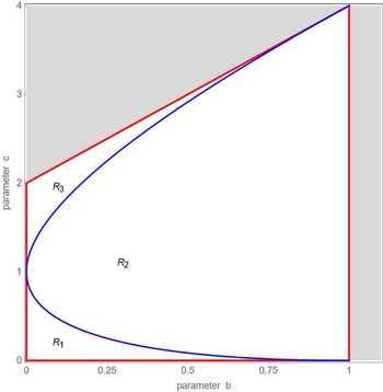


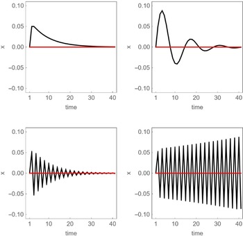


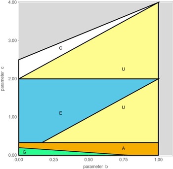


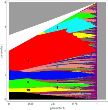


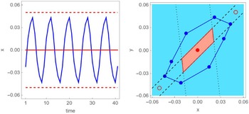


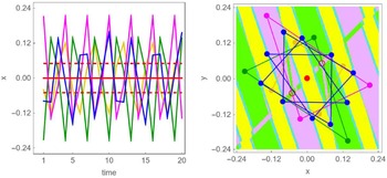


 Open access