


1. Introduction
Sensitive topics abound in social sciences where subjects are often unwilling to reveal their true preferences or behaviors (Blair et al., Reference Blair, Coppock and Moor2020). Recent innovations in statistical methodology have made tremendous advances in reducing sensitivity bias with the design and analysis of indirect questioning techniques (see, e.g., Conley and McCabe, Reference Conley and McCabe2011; Coutts and Jann, Reference Coutts and Jann2011; Rosenfeld et al., Reference Rosenfeld, Imai and Shapiro2016; Yamaguchi, Reference Yamaguchi2016). List experiments, in particular, have become a highly popular tool for social science research. While these experimental designs help reduce bias, they are not without cost. It is a well-known problem that estimates from list experiments lack statistical efficiency and are therefore, often less precise than desired or useful in samples of conventional size (Glynn, Reference Glynn2013; Blair et al., Reference Blair, Coppock and Moor2020).Footnote 1
In this paper, we address the inefficiency problem of list experiments head-on and present an informative Bayesian approach that combines indirect measures with prior evidence. One great benefit of the Bayesian approach is the ability to include additional information in a straightforward manner via prior distributions (Western and Jackman, Reference Western and Jackman1994; Gill and Walker, Reference Gill and Walker2005; Jackman, Reference Jackman2009; Gill, Reference Gill2015). Specifying informed priors amounts to a principled combination of information, which not only increases the efficiencyFootnote 2 of model estimates, but leads to an improved theoretical understanding of sensitive preferences and behaviors of political relevance.
Our contribution is thus fourfold. First, we improve the study of sensitive topics in social sciences by advancing the usability of list experiments. The inefficiency problem has limited a wider use of list experiments because it demands very large sample sizes that come with increased costs (Blair et al., Reference Blair, Coppock and Moor2020). As a result, many scholars turn back to direct survey questions, trading efficiency gains for bias. We demonstrate that the inefficiency of list experiments can be greatly reduced with readily available prior information.
Second, we connect the literature on list experiments to recent advances in survey methodology that combine probability and non-probability samples (Sakshaug et al., Reference Sakshaug, Wiśniowski, Ruiz and Blom2019; Wiśniowski et al., Reference Wiśniowski, Sakshaug, Ruiz and Blom2020; Jerit and Barabas, Reference Jerit and Barabas2023). This work faces a similar challenge of combining reliable but expensive information (probability samples) and less reliable but cheaper information (non-probability samples) with the ultimate goal to increase the accuracy of inferences. Specifically, we introduce the idea of “conjugate-distance” priors (Wiśniowski et al., Reference Wiśniowski, Sakshaug, Ruiz and Blom2020) to the analysis of list experiments.
Third, we unify several existing approaches to designing and analyzing list experiments under a single common framework. This is particularly useful, because mastering the many techniques scattered throughout the literature (e.g., Droitcour et al., Reference Caspar, ML, TL, W, TM, Biemer, Groves, Lyberg, Mathiowetz and Sudman1991; Blair et al., Reference Blair, Imai and Lyall2014; Aronow et al., Reference Aronow, Coppock, Crawford and Green2015; Chou et al., Reference Chou, Imai and Rosenfeld2020) places a high demand on applied researchers to learn multiple disparate approaches that were developed independently along with the accompanying software tools. By proposing a single Bayesian framework for list experiments, we generalize these existing approaches and only require users to do one thing: to specify prior distributions—regardless of the type of information or model class they would like to use. Our approach even allows for any combination of previous techniques by sequential Bayesian updating. An accompanying software package, bayeslist, which implements the proposed methods of this paper for easy use by applied researchers, is available in the Comprehensive R Archive Network.
Fourth, while social scientists have embraced Bayesian simulation methods as estimation tools for complicated models for quite some time (e.g., Jackman, Reference Jackman2000), they have been much more reluctant to tap into the full potential of the Bayesian approach by leveraging informed prior distributions. Instead, these “Bayesians of convenience” (Gill, Reference Gill2015) have defaulted to diffuse and often uniform prior forms. Early exceptions are Western and Jackman (Reference Western and Jackman1994) who use historical data and Gill and Walker (Reference Gill and Walker2005) who elicit expert knowledge to inform regression models. Similar in spirit, Glynn and Ichino (Reference Glynn and Ichino2015), Humphreys and Jacobs (Reference Humphreys and Jacobs2015), and Pérez Bentancur and Tiscornia (Reference Bentancur and Tiscornia2023) show how qualitative and quantitative evidence can be integrated to improve causal inference. We add to this literature by proposing Bayesian information integration for sensitive questions. Specifically, we introduce new data-derived sources for informative priors, show that they are often readily available and much easier to specify, and demonstrate how to mitigate concerns with biased priors. This latter point is especially valuable to dispel widespread concerns of “prior skeptics.” Thus, our contribution also encourages the wider use of informative priors in social science research.
2. Informative priors and list experiments
The utility of list experiments crucially depends on how much information is available for the analysis. Without a sufficiently large sample size, a biased direct question may be as good as or even better than a less biased but also less accurate list experiment (Blair et al., Reference Blair, Coppock and Moor2020; Li and Van den Noortgate, Reference Jiayuan and Van den Noortgate2022). The efficiency problem of list experiments has attracted great attention, but existing solutions are scattered in the literature and often developed in parallel. For example, different variance reduction strategies have been proposed, including: double list experiments (Miller, Reference Miller1984; Droitcour et al., Reference Caspar, ML, TL, W, TM, Biemer, Groves, Lyberg, Mathiowetz and Sudman1991), negatively correlated control items (Miller, Reference Miller1984; Glynn, Reference Glynn2013), combining list and endorsement experiment designs (Blair et al., Reference Blair, Imai and Lyall2014), combining list and direct question designs (Aronow et al., Reference Aronow, Coppock, Crawford and Green2015), and using auxiliary information (Chou et al., Reference Chou, Imai and Rosenfeld2020).
Thus, while some approaches focus on refinements of list experiments at the design stage, others attempt improvements at the analysis stage when data have already been collected. The former approach is subject to ex-post evaluation and can be very costly when the results are unsatisfying, and experiments have to be re-run. The latter, while arguably much cheaper, requires the mastering of multiple techniques that were developed separately and come with different software packages. All of this can be quite demanding for applied researchers.
Against this background, it would be desirable to have a single framework for the analysis of list experiments that is simple, accurate, and cost-efficient, and that can be done post hoc by combining already existing information rather than collecting more data. We propose such a framework based on the idea of Bayesian information updating that is able to incorporate various types of prior information for different models into the analysis of sensitive questions. Thereby, it simplifies the task of improving list experiment analysis by finding available external information and specifying priors.
2.1. Notation
2.1.1. List experiments
In a list experiment with  $N$ respondents, individual $i$ is randomly assigned to the control group ( $T_{i}=0$) and receives $J$ control items or to the treatment group ( $T_{i}=1$) and receives $J+1$ items by adding the sensitive item. The latent $Z^*_{i}$ indicates whether the respondent provides an affirmative answer to the sensitive item, and the latent variable $Y^*_i$ gives the number of affirmative answers to the control items. Respondents in the treated condition only reveal the aggregated outcome denoted by $Y_{i}$, which is the sum of the two latent variables.
2.1.2 Simple analysis of list experiments
The prevalence of the sensitive item,  $\pi$, can be obtained by a simple non-parametric differences-in-means estimator:
 \begin{equation}
\hat{\pi} = \frac{1}{N_1}\sum_1^{N}T_iY_{i} - \frac{1}{N_0}\sum_1^{N}(1 - T_i)Y_{i},
\end{equation}
\begin{equation}
\hat{\pi} = \frac{1}{N_1}\sum_1^{N}T_iY_{i} - \frac{1}{N_0}\sum_1^{N}(1 - T_i)Y_{i},
\end{equation} where  $N_1$ and $N_0$ are the number of respondents in the treatment and control group, respectively. The variance of the estimated prevalence $\hat{\pi}$ from this difference-in-means estimator (under a balanced list experiment design) is given as:
 \begin{equation}
\sigma^2_\text{list} =
\frac{1}{N - 1}\left\{\underbrace{\pi(1 - \pi)}_\text{Variance of sensitive item} + \underbrace{4\text{Var}(Y_i^*) + 4\text{Cov}(Y_i^*,Z^*)}_\text{Variance of and covariance with control items} \right\},
\end{equation}
\begin{equation}
\sigma^2_\text{list} =
\frac{1}{N - 1}\left\{\underbrace{\pi(1 - \pi)}_\text{Variance of sensitive item} + \underbrace{4\text{Var}(Y_i^*) + 4\text{Cov}(Y_i^*,Z^*)}_\text{Variance of and covariance with control items} \right\},
\end{equation} which consists of a variance component of the true prevalence  $\pi$, and variance and covariance components of the control items (Blair et al., Reference Blair, Coppock and Moor2020). Thus, the variance of the list experiment estimator is almost always larger than that of the direct question estimator, the extent to which depends on the variance of the control items and the correlation between sensitive and control items.
2.1.3 Regression models for list experiments
Recent innovations greatly improve the utility of list experiments by modeling answers in the context of regression models (Corstange, Reference Corstange2009; Imai, Reference Imai2011; Blair and Imai, Reference Blair and Imai2012; Imai et al., Reference Imai, Park and Greene2015; Eady, Reference Eady2017). While we obviously cannot observe individual answers to the sensitive item, the list experiment allows us to identify the joint distribution of the latent sensitive answer and the control items,  $P(Y^*_{i},Z^*_{i})$, if certain assumptions are met (randomization, no design effect, no liars) (Glynn, Reference Glynn2013). This possibility is then exploited in a multivariate modeling strategy that simultaneously models the response to the sensitive item and the control items.
Our focus here is the canonical sensitive item outcome model, where the answer to the sensitive item is regressed on and potentially explained by covariates (Imai, Reference Imai2011; Blair and Imai, Reference Blair and Imai2012). But our Bayesian approach also applies to alternative models, such as the sensitive item predictor model, where the answer to the sensitive item is entered as explanatory variable for some outcome of interest (Imai et al., Reference Imai, Park and Greene2015) or the sensitive item misreporting model which models misreporting of the sensitive item (Eady, Reference Eady2017).
2.1.4 Submodel for sensitive item
The core of all regression models for list experiments is the probability of affirming the sensitive item, i.e., its prevalence  $\pi$:
 \begin{equation}
\hat{\pi}_i = P(Z^*_{i} = 1 | \boldsymbol{X}_i) = g(\boldsymbol{X}_i;\boldsymbol{\delta}).
\end{equation}
\begin{equation}
\hat{\pi}_i = P(Z^*_{i} = 1 | \boldsymbol{X}_i) = g(\boldsymbol{X}_i;\boldsymbol{\delta}).
\end{equation} In this equation,  $\boldsymbol{X}_i$ is a vector of covariates for individual respondent $i$ and $\boldsymbol{\delta}$ is a vector of coefficients associated with the covariates. The probability is usually modeled using a logistic transformation on the linear combination of $\boldsymbol{X}_i$ and $\boldsymbol{\delta}$:
 \begin{equation}
g(\boldsymbol{X}_i;\boldsymbol{\delta}) = \text{logit}^{-1}(\boldsymbol{X}_i'\boldsymbol{\delta}).
\end{equation}
\begin{equation}
g(\boldsymbol{X}_i;\boldsymbol{\delta}) = \text{logit}^{-1}(\boldsymbol{X}_i'\boldsymbol{\delta}).
\end{equation}2.1.5 Submodel for control items
The probability of the number of affirmative answers to the control items is modeled in a similar way except that it uses a beta-binomial with  $J$ trials (i.e., the number of control items) and relates the outcome to a set of coefficients $\boldsymbol{\psi}$:
 \begin{equation}
P(Y^*_i = y | \boldsymbol{X}_i, Z^*_{i}, J) = h(y| \boldsymbol{X}_i, Z^*_{i}, J; \boldsymbol{\psi}),
\end{equation}
\begin{equation}
P(Y^*_i = y | \boldsymbol{X}_i, Z^*_{i}, J) = h(y| \boldsymbol{X}_i, Z^*_{i}, J; \boldsymbol{\psi}),
\end{equation} where  $h(\cdot)$ is the probability mass function of a beta-binomial distribution (Blair and Imai, Reference Blair and Imai2012). Due to the mixture structure of the likelihood, the coefficients, $\boldsymbol{\psi}$, also depend on the values of $Z^*_i$, although a common assumption is to simply set $\boldsymbol{\psi_{0}}=\boldsymbol{\psi_{1}}$ for the treatment and control groups.
2.1.6 Likelihood
Depending on the treatment condition  $T_i$, observed outcome $Y_i$, and latent variables $Z^*_i$ and $Y^*_i$, the observed-data likelihood functions of models for list experiments are combinations of the above mentioned probabilities, yielding a complicated mixture structure. More technical details and likelihood functions for these models can be found in the Supplementary Material A. We also refer readers to Imai (Reference Imai2011), Imai et al. (Reference Imai, Park and Greene2015) and Eady (Reference Eady2017). For Bayesian versions of these models of list experiments, we now require prior distributions for their unknown parameters of interest, e.g., $P(Z^*, \boldsymbol{\delta}, \boldsymbol{\psi})$. This is what we discuss next.
3. Combining list experiments with prior evidence: an informative Bayesian approach
The statistical analysis of list experiments suffers from what Western and Jackman (Reference Western and Jackman1994) have called the “weak data problem,” where a lack of sufficient information leads to high variances. The solution is therefore to bring in more information via prior distributions. Prior distributions are simply formal statements of the existing information a researcher brings to the analysis. That priors may impact statistical results is a long-standing concern with Bayesian analysis, which unfortunately has kept social scientists from exploiting the benefits of systematically including existing information into their models (see Gill and Walker (Reference Gill and Walker2005) and Western and Jackman (Reference Western and Jackman1994) for exceptions). We argue instead that researchers should embrace informative priors to strengthen their inferences on sensitive behaviors.
Although extant research has proposed Bayesian methods for list experiments (Blair and Imai, Reference Blair and Imai2012; Rosenfeld et al., Reference Rosenfeld, Imai and Shapiro2016; Blair et al., Reference Blair, Chou and Imai2019), it only relies on Bayesian simulation algorithms, but does not incorporate informative priors. Studies on sensitive questions that have incorporated prior information, are either not applicable to the analysis of list experiments (e.g., for endorsement experiments, see Groenitz (Reference Groenitz2015) and Chou et al. (Reference Chou, Imai and Rosenfeld2020)), or constrained to very specific types of prior data or prior distributions (Blair et al., Reference Blair, Imai and Lyall2014; Liu et al., Reference Liu, Tian, Qin and Tang2019), which limits their overall applicability. Groenitz (Reference Groenitz2014) proposed to incorporate priors for the analysis of list experiments without a control group. Blair et al. (Reference Blair, Imai and Lyall2014) propose a specific Bayesian procedure to combine list and endorsement experiments. Aronow et al. (Reference Aronow, Coppock, Crawford and Green2015) introduce a nonparametric estimator that combines list experiments with direct questions, but their non-Bayesian approach is restricted to prevalence estimates and does not extend to multivariate analysis or other sources of prior information.
Our approach is fully Bayesian and presents a generalized framework for incorporating prior information in regression models of list experiments. Our approach is not only readily adaptable to a) many different types of prior information (e.g., direct items (Aronow et al., Reference Aronow, Coppock, Crawford and Green2015) or auxiliary information (Chou et al., Reference Chou, Imai and Rosenfeld2020) from historic sources (Western and Jackman, Reference Western and Jackman1994) or experts (Gill and Walker, Reference Gill and Walker2005), etc.) but also b) to different model types like the sensitive item outcome (Blair and Imai, Reference Blair and Imai2012), the sensitive item predictor (Imai et al., Reference Imai, Park and Greene2015) and the misreporting model (Eady, Reference Eady2017). It also easily handles c) more specialized list experiment designs such as the double experiments (Droitcour et al., Reference Caspar, ML, TL, W, TM, Biemer, Groves, Lyberg, Mathiowetz and Sudman1991) and even allows for d) the combination of list experiments with other types of experiments (Gerber and Green, Reference Gerber and Green2012; Blair et al., Reference Blair, Imai and Lyall2014). More generally, our contribution is to demonstrate the benefits of a fully Bayesian approach and to encourage the wider use of informative priors in social science research.
In what follows, we first show why informative priors work and where they come from. The next section then illustrates in great detail how Bayesian analysis of list experiments is done in practice and how it changes our understanding of sensitive topics.
3.1. The case for informative priors
Bayesian inference offers a disciplined routine to incorporate prior information into the model estimation process via Bayes’ rule. Remember that this rule uses probability statements on how to update prior beliefs about unknown quantities and model parameters with the likelihood of the data to form posterior beliefs (Jackman, Reference Jackman2009; Gill, Reference Gill2015). The distinction between uninformative or vague priors and informative priors refers to the choice of the parameters and the shape of their respective probability distributions. In the absence of prior information, one could set the mean of the distribution to zero and choose a large variance, resulting in a flat distribution. Model estimates are then almost fully determined by the likelihood alone. But this misses a valuable opportunity to incorporate additional information by specifying the prior mean and variance in more precise terms, which results in a more narrow prior distribution.
To provide some intuition for why the incorporation of prior information increases the efficiency of list experiments, we return to the simple difference-in-means estimator (Equation 1). By relying on the central limit theorem, we may treat the estimates as normally distributed with mean equal to the true prevalence  $\pi$ and variance of the sampling distribution $\sigma^2_\text{list}$, i.e., $\hat{\pi}\sim \mathcal{N}(\pi, \sigma^2_\text{list})$ (cf. Gerber and Green, Reference Gerber and Green2012). Additional outside information on the prevalence may be specified as a prior distribution that also takes a normal form, i.e., $\pi\sim \mathcal{N}(\pi_{0}, \sigma^2_\text{prior})$, where $\pi_{0}$ is the prior prevalence suggested by the external information source and $\sigma^2_\text{prior}$ expresses our uncertainty about this prevalence.
Based on a standard result in conjugate Bayesian analysis, the combination of normally distributed data and a normal prior yields a normally distributed posterior with the following precision,  $\tau_\text{posterior}$:Footnote 3
 \begin{equation}
\tau_\text{posterior} = N \times {\tau_\text{list}} + {\tau_\text{prior}} .
\end{equation}
\begin{equation}
\tau_\text{posterior} = N \times {\tau_\text{list}} + {\tau_\text{prior}} .
\end{equation} The above equation summarizes the three main factors influencing estimation efficiency, namely: the sample size, the data precision, and the prior precision. First, everything else equal, the larger the sample size  $N$, the higher the posterior precision. Second, the higher the precision of the list experiment denoted by $\tau_\text{list}$, the higher the posterior precision. The key ingredient is the third term, i.e., the prior precision $\tau_\text{prior}$. The more prior information we have, the higher the prior precision and therefore the overall posterior precision. Indeed, as long as the variance of the prior is not infinite, we will always have more efficiency by incorporating at least some prior evidence.Footnote 4
In addition to efficiency gains, another advantage of incorporating prior information is to avoid “inadvertently informative” priors. Remember that a prime interest lies in making inferences about the parameters  $\boldsymbol{\delta}$ in the submodel $g(\boldsymbol{X}_i;\boldsymbol{\delta})$ for the sensitive item and that it often takes the logistic form. Unfortunately, vague normal priors in logistic regression models may have unintended consequences (cf. Seaman III et al., Reference Seaman, John, John, Seaman and James2012; Northrup and Gerber, Reference Northrup and Gerber2018). Since the logit transformation is non-linear, large negative and large positive values yield transformed probabilities that are bimodal and bunch up against zero and one. The problem is more serious the larger the prior variance. Therefore, more “uninformative” priors on the logit scale may actually turn out to be highly informative on the probability scale (see Supplementary Material C for an illustration). This may be especially problematic for low-incidence sensitive items and weak data sets with few observations, where the prior is more influential. One solution is to reduce the prior variance, e.g., by specifying uninformative priors on the logit scale as $\mathcal{N}(0, 1)$, which translates roughly into a uniform prior on the probability scale (McElreath, Reference McElreath2018). Again, we suggest relying on informative priors with low variance instead. This way, the prior variance is not set in an ad-hoc fashion but guided by existing evidence.
We note that obtaining external information relevant to sensitive questions is often astoundingly easy. This is because it either already exists in direct numerical form or is an already existing element of the research design and therefore available “for free.” For instance, whilst potentially biased, prevalence rates of sensitive behaviors are usually available from governments, NGOs, or field experts, at least for some sub-populations. Many list experimental designs also include direct survey questions on the sensitive topic (Blair et al., Reference Blair, Coppock and Moor2020). Last, because different researchers usually conduct list experiments with similar sensitive questions for different populations or time points, information from previous list experiments can be used to inform the analysis of the current list experiment (see Gerber and Green (Reference Gerber and Green2012) for the integration of experiments).
3.2. Bayesian information integration
According to Bayes’ theorem, the joint posterior distribution of the main unknown parameters of interest—i.e., the latent sensitive attitude or behavior  $Z^*$ and the submodel coefficients $\boldsymbol\delta$ and $\boldsymbol\psi$—is obtained by conditioning on the observed outcome data $Y$, treatment status $T$ and set of control variables $\boldsymbol{X}$, as well as prior distributions for all unknowns via the generic statement:
 \begin{equation}
\underbrace{P(Z^*, \boldsymbol\delta, \boldsymbol\psi | \{\boldsymbol{X},Y, T\})}_\text{ Posterior} \propto \underbrace{P(\{\boldsymbol{X},Y, T\} |Z^*, \boldsymbol\delta, \boldsymbol\psi)}_\text{ Likelihood}\underbrace{P(Z^*, \boldsymbol\delta, \boldsymbol\psi)}_\text{ Prior} .
\end{equation}
\begin{equation}
\underbrace{P(Z^*, \boldsymbol\delta, \boldsymbol\psi | \{\boldsymbol{X},Y, T\})}_\text{ Posterior} \propto \underbrace{P(\{\boldsymbol{X},Y, T\} |Z^*, \boldsymbol\delta, \boldsymbol\psi)}_\text{ Likelihood}\underbrace{P(Z^*, \boldsymbol\delta, \boldsymbol\psi)}_\text{ Prior} .
\end{equation} While the prevailing maximum likelihood estimation of list experiments focuses on maximizing the likelihood  $P(\{\boldsymbol{X},Y, T\} |Z^*, \boldsymbol\delta, \boldsymbol\psi)$,Footnote 5 Bayesian inference instead multiplies it with the joint prior distribution for all unknown quantities $P(Z^*, \boldsymbol\delta, \boldsymbol\psi)$. The actual model estimation involves marginalizing the resulting posterior $P(Z^*, \boldsymbol\delta, \boldsymbol\psi | \{\boldsymbol{X},Y, T\})$ using MCMC or related statistical simulation algorithms. Since these are implemented in readily available general purpose software such as STAN or JAGS (Plummer, Reference Plummer2003; Carpenter et al., Reference Carpenter, Gelman, Hoffman, Lee, Goodrich, Betancourt, Brubaker, Guo, Peter and Riddell2017), we do not address them here.Footnote 6 Instead, our focus is specifically on the role of the prior distribution and its effects.
The prime interest when analyzing list experiments usually centers on the prevalence of the sensitive item  $Z^*$ and/or the coefficients in the sensitive outcome equation, $\boldsymbol\delta$. Given the model structure, we may factor the joint prior distribution into its component marginal and conditional prior distributions:Footnote 7
 \begin{equation}
P(Z^*, \boldsymbol\delta, \boldsymbol\psi) = P(\boldsymbol\psi)P(\boldsymbol\delta|Z^*)P(Z^*) = P(\boldsymbol\psi)P(Z^*|\boldsymbol\delta)P(\boldsymbol\delta).
\end{equation}
\begin{equation}
P(Z^*, \boldsymbol\delta, \boldsymbol\psi) = P(\boldsymbol\psi)P(\boldsymbol\delta|Z^*)P(Z^*) = P(\boldsymbol\psi)P(Z^*|\boldsymbol\delta)P(\boldsymbol\delta).
\end{equation} This factorization shows that we can specify informative priors for  $Z^*$ or $\boldsymbol\delta$ independently of priors for $\boldsymbol\psi$, which will usually be of the uninformative kind. Because prior information on one parameter propagates to another via the conditional, we are able to formulate a prior for either $Z^*$ or $\boldsymbol{\delta}$ while simultaneously informing the other parameter. This is a convenient feature as it allows us to select an appropriate prior depending on what source of information is available. Sometimes, prior information on the latent prevalence $Z^*$ will be available (see our real-world example in Supplementary Material F). In other instances, as in the real-world examples discussed in Section 4, prior information will directly refer to the coefficients $\boldsymbol{\delta}$ in the sensitive item outcome model.
3.3. Dispelling prior concerns
Many researchers are skeptical of using prior information because of the suspicion that doing so injects “subjectivity” into the analysis instead of “letting the data speak” by itself. This concern has at least three components: a) a general concern with “subjectivity” in data analysis which seems to violate “objective” scientific practice, b) a particular concern with the sources of prior information which may seem arbitrary, and c) a more specific concern with the deliberate use of information that is already known to be biased. We dispel these concerns as follows.
First, and as has been noted again and again, all decisions in statistical modeling are in a sense “subjective” and require justification. This includes, among many others, distributional assumptions about the data generation process, which variables to include in the model and with which functional form. That “researcher degrees of freedom” are vast and have direct implications for results is recognized in the recent discussion about the credibility crisis in science (Simmons et al., Reference Simmons, Nelson and Simonsohn2011; Breznau et al., Reference Breznau, Rinke, Wuttke, Nguyen, Adem, Adriaans, Alvarez-Benjumea, Andersen, Auer, Azevedo and Bahnsen2022). Thus, prior distributions are not qualitatively different from the many other modeling assumptions researchers make.
Second, the source of information used in prior construction is far from subjective but is often itself based on data. In informative priors, there are two major sources: “expert opinion” and “historic data.” In our approach, we focus on the latter and suggest new sources for such already existing information, notably common elements of list experimental designs themselves, such as direct items. At its core, Bayes rule provides a principled mechanism to combine existing information. So instead of injecting “subjectivity,” we actually make better use of the available evidence and rely even more on data than we would without informative priors.
Third, regarding the concerns with the biased nature of the information used, we respond in two ways. First, it is a well-known result that the accuracy of a statistical estimator (expressed as mean squared error) can be decomposed into bias and variance, i.e.,  $MSE = Bias^2 + Variance$ (e.g., James et al., Reference James, Witten, Hastie and Tibshirani2013). This re-expresses the well-known variance-bias tradeoff and suggests that the costs of accepting a little bias may be completely offset by the benefit of a decrease in variance. The overall net effect is improved accuracy. Second, we provide an explicit mechanism to deal with biased prior information via the so-called conjugate-distance prior (Wiśniowski et al., Reference Wiśniowski, Sakshaug, Ruiz and Blom2020), and show that it yields unbiased estimates on average in the next section.
3.4. Bias correction in prior specification
While trading bias for increased efficiency may be a good bargain, we anticipate that many researchers will be hesitant to incorporate potentially biased information in their models of list experiments. This worry is clearly warranted if both the bias’s direction and magnitude are unknown. Fortunately, this is not a concern in the context of list experiments, where we often have information on the direction and size of the bias by design. In the following, we will demonstrate how to exploit this additional knowledge for bias correction in prior specification.
Our solution is inspired by recent advances in survey methodology that seek to combine inferences from probability-based and non-probability samples (Sakshaug et al., Reference Sakshaug, Wiśniowski, Ruiz and Blom2019; Wiśniowski et al., Reference Wiśniowski, Sakshaug, Ruiz and Blom2020; for a concise review, see Jerit and Barabas Reference Jerit and Barabas2023). This research faces the related challenge of combining reliable but sparse data from expensive probability-based samples with less reliable, probably biased but abundant, cheap data from non-probability samples (e.g., commercial access panels). Using a Bayesian framework, this amounts to treating the probability-based sample as the “likelihood” and the non-probability sample as “prior information.” Their combination results in posterior survey estimates that have less variance (Sakshaug et al., Reference Sakshaug, Wiśniowski, Ruiz and Blom2019). Just like our approach, this involves the deliberate incorporation of potentially biased information in the form of a prior to yield more efficient posterior estimates. Specifically, we consider the so-called “conjugate-distance” prior introduced in this literature (Wiśniowski et al., Reference Wiśniowski, Sakshaug, Ruiz and Blom2020).
The conjugate-distance prior allows us to gain efficiency, while bounding the influence of biased information on the posterior. Let us assume a normal prior for the coefficient of covariate  $k$, with prior mean equal to the point estimate $\hat{\delta}_{D,k}$ from a direct item model. While biased, this still represents the best knowledge we have before running the sensitive item model. We then run the sensitive item model with an uninformative prior to get the unbiased estimate $\hat{\delta}_{S,k}$. The key ingredients of the conjugate-distance prior are the distance between $\hat{\delta}_{D,k}$ and $\hat{\delta}_{S,k}$, and the standard errors $\hat{\sigma}_{D,k}$ from the estimation of the direct items.
The intuition behind this prior specification is as follows. Whenever the difference between the potentially biased  $\hat{\delta}_{D,k}$ and the unbiased $\hat{\delta}_{S,k}$ is smaller than the standard error $\hat{\sigma}_{D,k}$ from the direct item, we can just use this standard error to shrink the prior distribution. Whenever there is greater disagreement between the biased and unbiased coefficient estimates, we instead let the prior variances be proportional to the squared differences between the two sets of estimates. The prior variance is thus calculated as
 \begin{equation}
\hat{\sigma}_{P,k}^2 = \text{max}\left[(\hat{\delta}_{D,k} - \hat{\delta}_{S,k})^2, \hat{\sigma}_{D,k}^2\right],
\end{equation}
\begin{equation}
\hat{\sigma}_{P,k}^2 = \text{max}\left[(\hat{\delta}_{D,k} - \hat{\delta}_{S,k})^2, \hat{\sigma}_{D,k}^2\right],
\end{equation}and for the complete prior specification, we use
 \begin{equation}
\delta_k \sim \mathcal{N}(\hat{\delta}_{D,k}, \hat{\sigma}_{P,k}^2).
\end{equation}
\begin{equation}
\delta_k \sim \mathcal{N}(\hat{\delta}_{D,k}, \hat{\sigma}_{P,k}^2).
\end{equation}Thereby, we allow the amount of sensitivity bias to rescale the prior variance and prevent the danger that the posterior distribution will be dominated by biased estimates.Footnote 8
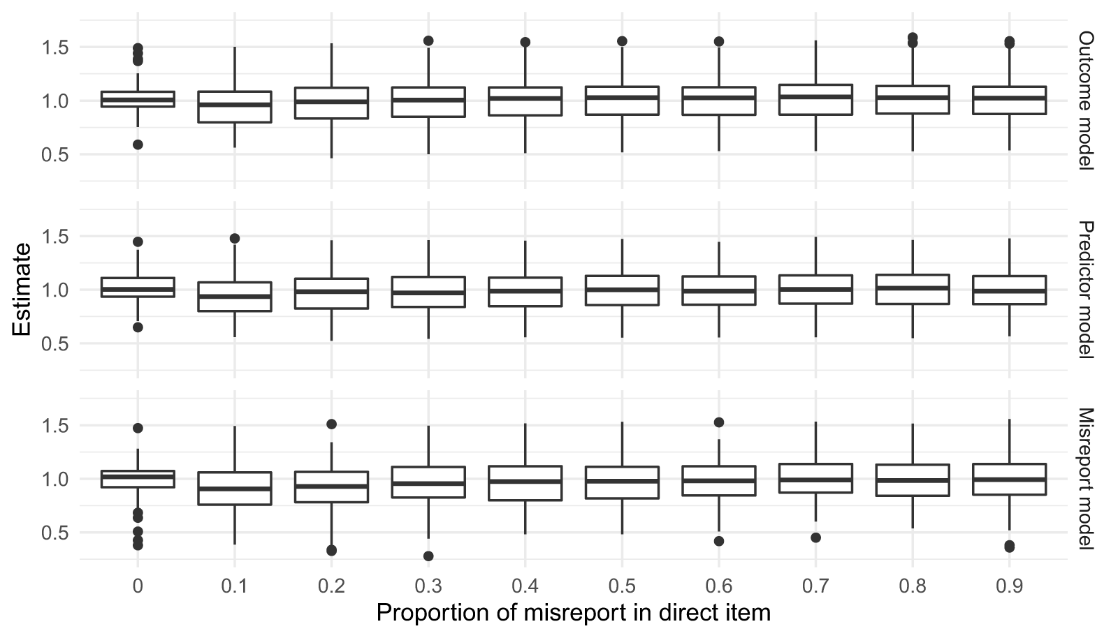
To demonstrate that the conjugate-distance prior indeed works as intended, we ran a detailed simulation study (see Supplementary Material D for details on the exact set-up of this simulation exercise). Figure 1 shows the simulation results of using informative priors based on biased direct items scaled by the conjugate-distance method. The key takeaway is that regardless of how likely the respondents are to misreport their answers to a direct question, the resulting estimates of our suggested approach remain unbiased on average.
Estimates using conjugate-distance priors as misreport proportion in direct items increases (true coefficient value equals one).

A possible remaining concern with the conjugate-distance prior is an alleged “double use” of the same data. But apart from the fact that no such concerns are raised in the related survey literature (e.g., Sakshaug et al., Reference Sakshaug, Wiśniowski, Ruiz and Blom2019; Wiśniowski et al., Reference Wiśniowski, Sakshaug, Ruiz and Blom2020; Jerit and Barabas, Reference Jerit and Barabas2023), we note that almost all common prior modeling techniques are implicitly motivated by a reference likelihood (Gelman et al., Reference Gelman, Simpson and Betancourt2017). In fact, our approach has a close connection to “empirical Bayes” (EB) methods. EB methods have in common that they empirically estimate some part of the Bayesian procedure (see Efron (Reference Efron, Berger, Meng, Reid and Xie2024) for a recent overview). In this sense, our use of the “conjugate-distance prior” can also be labeled EB because it uses empirical data to adjust the variance of the prior distribution. We provide a more detailed discussion of the “double-use” problem and why it is easy to dispel in Supplementary Material E.
4. Illustration of Bayesian analysis of list experiments using informative priors
We now illustrate our Bayesian approach to list experiments in a real-world application. Specifically, we identify commonly available prior evidence for list experiments, detail the steps needed to quantify prior evidence as prior probability distributions, and demonstrate how combining list experiments with prior evidence improves our substantive understanding of sensitive topics in the social sciences.
A very useful and straightforward source of prior information is direct survey items about the sensitive issue (Aronow et al., Reference Aronow, Coppock, Crawford and Green2015). Indeed, around one hundred of the list experiment studies summarized in Blair et al. (Reference Blair, Coppock and Moor2020) also asked respondents direct sensitive questions. These direct questions are usually asked for the purpose of comparison and are often biased due to social desirability. What is less emphasized is the fact that these direct questions are often biased in a systematic way and thus, still provide valuable information that can be exploited (Aronow et al., Reference Aronow, Coppock, Crawford and Green2015).
As an illustrative example, we consider the study by Gonzalez-Ocantos et al. (Reference Gonzalez-Ocantos, De Jonge, Meléndez, Osorio and Nickerson2012) on vote buying in Nicaragua. Political clientelism, where electoral support is traded for particularistic favors, is not only a problem in Latin American politics but plagues many democracies around the world (Mares and Young, Reference Mares and Young2016). Because of the sensitive nature of vote buying, Gonzalez-Ocantos et al. (Reference Gonzalez-Ocantos, De Jonge, Meléndez, Osorio and Nickerson2012) use a list experiment that elicits whether respondents were ever offered a gift for their vote. They also include two direct survey questions asking about “individual gifts” and “neighborhood gifts.” The study shows that while less than 3% report individual vote buying behavior when asked directly, some 18% report vote buying behavior in their neighborhood. The list experiment yields an even higher prevalence rate of 24%. But next to the question of the true extent of this form of political clientelism, there is also considerable debate about the characteristics of voters who are most likely to experience and respond to such economic inducements (Stokes, Reference Stokes2005; Nichter, Reference Nichter2008; Mares and Young, Reference Mares and Young2016). As we will demonstrate, including direct items as prior information also has the potential to change the substantive conclusions regarding the determinants of vote buying.
We would like to stress that our Bayesian framework for the analysis of list experiments also applies to a wider range of data situations and is not restricted to the use of direct questions as prior information. In the Supplementary Material, we provide two more real-world applications. The first demonstrates the use of auxiliary information on the prevalence of the sensitive item, including in the form of a “conjugate-distance” prior (see Supplementary Material F). The second application illustrates how our Bayesian approach can be used to analyze a specialized design called the “double-list experiment,” providing a framework for combining different experiments via the use of informative priors (see Supplementary Material G).
4.1. Prior specification and sequential Bayesian updating
To incorporate direct items as prior information into the estimation of list experiments, we suggest the following simple procedure to derive prior distributions for the coefficients in the sensitive item outcome model:
• Prior Specification Using Direct Items
• Step 1. Run the model without priors and using direct item ${D}$ as the outcome to obtain coefficient estimates
$\hat{\delta}_{{D},k}$ and standard errors
$\hat{\sigma}_{{D},k}$ for each covariate
$k \in \{0,\cdots, K\}$, where
$K$ is the number of covariates and
$k = 0$ for the intercept.
${D}$ as the outcome to obtain coefficient estimates
$\hat{\delta}_{{D},k}$ and standard errors
$\hat{\sigma}_{{D},k}$ for each covariate
$k \in \{0,\cdots, K\}$, where
$K$ is the number of covariates and
$k = 0$ for the intercept.• Step 2. Use these estimates to inform the location and spread of the priors for the sensitive item outcome model of the list experiment, e.g.,
$\delta_k \sim \mathcal{N}(\hat{\delta}_{{D},k}, \hat{\sigma}^2_{{D},k})$ for each covariate
$k$.


Since a Bayesian model with the correctly bounded uniform priors is equivalent to a likelihood model without priors (Diaconis and Freedman, Reference Diaconis and Freedman1986, Reference Diaconis and Freedman1990), the first step is to simply run the desired model without priors but using the direct item,  ${D}$, as the outcome. Because this is usually a binary variable, a popular model choice is to use logistic regression:
 \begin{equation}
P({D} = {1})=\text{logit}^{-1}(\boldsymbol{X}_i'\boldsymbol{\hat{\delta}}_{{D}}).
\end{equation}
\begin{equation}
P({D} = {1})=\text{logit}^{-1}(\boldsymbol{X}_i'\boldsymbol{\hat{\delta}}_{{D}}).
\end{equation} This is convenient because we can now directly work with these model estimates  $\boldsymbol{\hat{\delta}}_{{D}}$ and their associated standard errors $\boldsymbol{\hat{\sigma}}_{{D}}$ to form our prior distributions on the logit scale without having to worry about transformations. More generally, in the presence of $k$ covariates, logistic regression based on direct items will yield a prior for the coefficient of the k-th covariate $\delta_k$ with mean $\hat{\delta}_{{D},k}$ and the standard error $\hat{\sigma}_{{D},k}$ (note the use of subscripts, e.g., $D$, to distinguish priors and model parameters). Relying on the central limit theorem, we are able to assume that coefficients in the sensitive item outcome model will be normally distributed and thus pick a prior distribution for $\delta_k$ which also follows a normal distribution.
In the second step, we can impose this normal distribution as an informative prior on  $\delta_k$ in the sensitive item outcome model, simply plugging in the coefficient estimates and (squared) standard errors as the required means and variances:Footnote 9
 \begin{equation}
\delta_k \sim \mathcal{N}(\hat{\delta}_{{D},k}, \hat{\sigma}_{{D},k}^2),
\end{equation}
\begin{equation}
\delta_k \sim \mathcal{N}(\hat{\delta}_{{D},k}, \hat{\sigma}_{{D},k}^2),
\end{equation}where the actual derivation of the posterior distribution and its marginalization are then left to the statistical software. Note that in contrast to the method described by Aronow et al. (Reference Aronow, Coppock, Crawford and Green2015), the procedure outlined above allows for multivariate analysis of list experiments and is also applicable when direct questions and list experiments are answered by distinct sets of respondents or part of completely independent studies.
To make things more concrete, we turn to the vote buying example. Which voter characteristics explain whether they received a gift or favor in exchange for their vote? A logistic regression model for the direct report of individual gift receiving behavior yields the following coefficient estimates (with standard errors in parentheses):
 \begin{eqnarray*}
P(\text{Individual.Gift}=1)
= \text{logit}^{-1}(-3.58 (1.07)
+ 1.31 (0.56) \times \text{Support.FSLN} \\
-0.16 (0.87) \times \text{Support.PLC}
+ 1.20 (0.63) \times \text{Very.Poor}
+ 0.62 (0.60) \times \text{Poor} \\
-0.33 (0.29) \times \text{Education}
-0.46 (0.31) \times \text{Age}
-0.40 (0.43) \times \text{Male}).
\end{eqnarray*}
\begin{eqnarray*}
P(\text{Individual.Gift}=1)
= \text{logit}^{-1}(-3.58 (1.07)
+ 1.31 (0.56) \times \text{Support.FSLN} \\
-0.16 (0.87) \times \text{Support.PLC}
+ 1.20 (0.63) \times \text{Very.Poor}
+ 0.62 (0.60) \times \text{Poor} \\
-0.33 (0.29) \times \text{Education}
-0.46 (0.31) \times \text{Age}
-0.40 (0.43) \times \text{Male}).
\end{eqnarray*} Thus, based on this direct item model, we would conclude that voters’ socio-demographic characteristics have little to do with their susceptibility to vote buying. For instance, poor and very poor voters do not differ significantly from more well-off voters in admitting individual vote buying (logit coefficient  $\hat{\delta}_{{D},\text{Poor}}=0.62$ with standard error $\hat{\sigma}_{{D},\text{Poor}}=0.60$ and $\hat{\delta}_{{D}, \text{Very.Poor}}=1.20$ with $\hat{\sigma}_{{D}, \text{Very.Poor}}=0.63$). But interestingly, party supporters of the leftist party Frente Sandinista de Liberación Nacional (FSLN) are markedly more likely to be targeted by politicians and their brokers ( $\hat{\delta}_{{D},\text{Support.FSLN}}=1.31$ with $\hat{\sigma}_{{D}, \text{Support.FSLN}}=0.56$).
This clearly is valuable information and suggests the following prior distributions for the coefficients of the sensitive item outcome model:Footnote 10
 \begin{eqnarray*}
\delta_\text{Intercept} \sim \mathcal{N}(-3.58, 1.07^2);&
\delta_\text{Support.FSLN} \sim \mathcal{N}(1.31, 0.56^2);&
\delta_\text{Support.PLC} \sim \mathcal{N}(-0.16, 0.87^2); \\
\delta_\text{Very.Poor} \sim \mathcal{N}(1.20, 0.63^2);&
\delta_\text{Poor} \sim \mathcal{N}(0.62, 0.60^2);&
\delta_\text{Education} \sim \mathcal{N}(-0.33, 0.29^2); \\
\delta_\text{Age} \sim \mathcal{N}(-0.46, 0.31^2);&
\delta_\text{Male} \sim \mathcal{N}(-0.40, 0.43^2).&
\end{eqnarray*}
\begin{eqnarray*}
\delta_\text{Intercept} \sim \mathcal{N}(-3.58, 1.07^2);&
\delta_\text{Support.FSLN} \sim \mathcal{N}(1.31, 0.56^2);&
\delta_\text{Support.PLC} \sim \mathcal{N}(-0.16, 0.87^2); \\
\delta_\text{Very.Poor} \sim \mathcal{N}(1.20, 0.63^2);&
\delta_\text{Poor} \sim \mathcal{N}(0.62, 0.60^2);&
\delta_\text{Education} \sim \mathcal{N}(-0.33, 0.29^2); \\
\delta_\text{Age} \sim \mathcal{N}(-0.46, 0.31^2);&
\delta_\text{Male} \sim \mathcal{N}(-0.40, 0.43^2).&
\end{eqnarray*} The resulting posterior distributions for all coefficients of the sensitive item model are presented in Figure 2 (Panel a). As is common practice, we summarize them in terms of prior means and 95% credible intervals. We also contrast them with the posterior estimates derived from a model with uninformative priors (i.e.,  $\delta_\text{k} \sim \mathcal{N}(0, 10^2)$ for all $k$), which therefore only reflects the information provided by the list experiment alone. It is immediately apparent that informed priors improve the efficiency. By using the direct item “individual gifts” as the prior information, the variance of the estimated prevalence was reduced by 45% compared to the estimation using an uninformative normal prior (Panel a). The second direct item “neighborhood gifts” produces an even higher variance reduction rate of 75% (Panel b). But before we turn to the substantive interpretation of these results, it is worth considering whether even more prior information can be brought to the analysis.
Comparison between estimates using uninformative (highlighted in gray) and informative priors (highlighted in orange) from direct items on vote buying (posterior means along with 95% credible intervals).

When there is more than one direct item available, one could include this additional information by sequentially updating the prior information with the following steps:
• Sequential Bayesian Updating for Several Direct Items
• Step 1. Run a model without priors and using the first direct item
${D}_{1}$ as the outcome to obtain coefficient estimates
$\hat{\delta}_{D_1,k}$ and standard errors
$\hat{\sigma}_{D_1,k}$ for each covariate
$k \in \{0,\cdots,K\}$ in the first direct item model.• Step 2. Repeat the following procedure to incorporate all available information up to the
$q$th direct item.For
$i$ from
$1$ to
$q-1$:(i) Use the estimates from the
$i$th direct item to produce informed priors for the next direct item model, e.g.,
$\delta_{D_{i+1},k} \sim \mathcal{N}(\hat{\delta}_{D_i,k}, \hat{\sigma}_{D_i,k}^2)$.(ii) Run a model with the above informed priors using the
$(i+1)$th direct item
${D}_{i+1}$ as outcome to obtain coefficient estimates
$\hat{\delta}_{D_{i+1},k}$ and standard errors
$\hat{\sigma}_{D_{i+1},k}$ for each covariate
$k$.• Step 3. Use the final estimates to inform the priors for the sensitive item outcome model of the list experiment, e.g.,
$\delta_k \sim \mathcal{N}(\hat{\delta}_{D_q,k}, \hat{\sigma}_{D_q,k}^2)$ for each covariate
$k$.


Applying the above procedure to the vote buying example, the estimates from the direct item on individual gift receiving behavior  ${D}_{1}$ can now be used to inform the model of the direct item on neighborhood gift receiving behavior ${D}_{2}$ (i.e., instead of $\delta_{k}$ we put the priors on $\delta_{D_2,k}$). Following the logic of sequential updating, the resulting coefficient estimates and standard errors can then, in turn, be used to inform the prior distributions for the coefficients of the sensitive item outcome model.
The informative priors that contain the information of two direct items ( ${D}_{1}$ and ${D}_{2}$) will have considerably smaller variances. For instance, the prior for the coefficient of FSLN support is now:
 \begin{equation*}
\delta_\text{Support.FSLN} \sim \mathcal{N}(0.45, 0.19^2),
\end{equation*}
\begin{equation*}
\delta_\text{Support.FSLN} \sim \mathcal{N}(0.45, 0.19^2),
\end{equation*} with variance  $\sigma_\text{Support.FSLN}^2=0.19^2$, which is much smaller than the prior variance suggested by the first direct item model alone, $\sigma_\text{Support.FSLN}^2=0.56^2$. Note that sequential updating yields exactly the same posterior as combining all information at the same time. Put differently, the order in which we update does not matter. Panel c of Figure 2 shows that incorporating both direct items significantly improves the efficiency of the list experiment analysis. Compared to Panels a and b, where only one direct item is incorporated, the variance of the posterior prevalence in Panel c is reduced by 82% with the inclusion of both direct items.
In addition to variance reduction for the estimated prevalence, the coefficient estimates also show a significant efficiency improvement when direct items are exploited as prior information. This in turn leads to substantively different results on the mechanisms of vote buying. A central question and long-standing debate in the literature concerns who is more likely to be targeted for vote buying: swing voters and those weakly opposed (Stokes, Reference Stokes2005; Stokes et al., Reference Stokes, Dunning, Nazareno and Brusco2013) or core party supporters (Nichter, Reference Nichter2008; Calvo and Murillo, Reference Calvo and Murillo2013; Albertus, Reference Albertus2015). Relying on the results of the list experiment alone, we find that there are no statistically reliable differences between these voter groups. The coefficient for supporters of the FSLN is -0.36 [-1.51, .078] and for supporters of the PLC -1.05 [-3.30, 0.87] (see Figure 2). Accordingly, Gonzalez-Ocantos et al. (Reference Gonzalez-Ocantos, De Jonge, Meléndez, Osorio and Nickerson2012), 210 conclude that there is “little support for Nichter’s (2008) argument that machines mainly target core supporters in an effort to buy turnout.”
But this conclusion may simply be due to the high variance and indeed changes as soon as we consider the direct item about neighborhood vote buying as prior evidence. By incorporating this additional piece of information into the model, we find that supporters of the center-right party Partido Liberal Constitucionalista (PLC) are reliably more susceptible to vote buying than independent voters (logit coefficient of 0.75 with 95% credible interval of [0.34, 1.14]). Sequentially updating the priors and therefore exploiting the information contained in both direct items leads to further substantive insights. Now, not only supporters of the PLC but also supporters of the FSLN are more likely to report being targeted for vote buying. Combining the list experiment with prior information lends support to the notion that it is core party supporters rather than swing voters who are approached by parties. This changes the substantive conclusion of the original study by Gonzalez-Ocantos et al. (Reference Gonzalez-Ocantos, De Jonge, Meléndez, Osorio and Nickerson2012) and suggests that the findings for Nicaragua in fact correspond to those in other Latin American countries such as Argentina (Nichter, Reference Nichter2008), Chile (Calvo and Murillo, Reference Calvo and Murillo2013), and Venezuela (Albertus, Reference Albertus2015).
4.2. Bias correction in prior specification
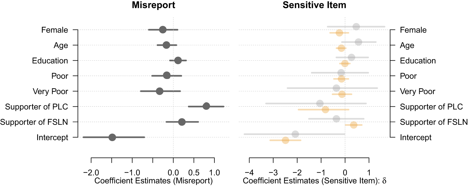
Despite the improved efficiency of our Bayesian approach, researchers may still be concerned about the potential bias of the direct item, which derives from voters’ tendency to under-report this particular behavior. To address this potential bias and provide a meaningful interpretation, we utilize the conjugate-distance prior.
To illustrate the conjugate-distance prior, we turn to a sensitive item misreporting model (Eady, Reference Eady2017), which adds a separate equation for misreporting to the sensitive outcome and control times equations (see Equation A3 in the Supplementary Material A for more details). For the coefficients in this misreporting equation,  $\boldsymbol{\gamma}$, we simply choose priors from a direct item model of “neighborhood gifts,” e.g.
 \begin{eqnarray*}
\gamma_\text{Support.PLC} \sim \mathcal{N}(0.35, 0.20^2), \\
\gamma_\text{Support.FSLN} \sim \mathcal{N}(0.79, 0.22^2).
\end{eqnarray*}
\begin{eqnarray*}
\gamma_\text{Support.PLC} \sim \mathcal{N}(0.35, 0.20^2), \\
\gamma_\text{Support.FSLN} \sim \mathcal{N}(0.79, 0.22^2).
\end{eqnarray*} Note that these priors are highly informative for misreporting because they explicitly capture respondents’ biased answering behavior. In contrast, for the coefficients in the sensitive outcome equation,  $\boldsymbol{\delta}$, we would instead want to correct for this known bias by specifying the following conjugate-distance priors
 \begin{eqnarray*}
\delta_\text{Support.PLC} \sim \mathcal{N}(0.35, \hat{\sigma}_{P,\text{Support.PLC}}^2), \\
\delta_\text{Support.FSLN} \sim \mathcal{N}(0.79, \hat{\sigma}_{P,\text{Support.FSLN}}^2),
\end{eqnarray*}
\begin{eqnarray*}
\delta_\text{Support.PLC} \sim \mathcal{N}(0.35, \hat{\sigma}_{P,\text{Support.PLC}}^2), \\
\delta_\text{Support.FSLN} \sim \mathcal{N}(0.79, \hat{\sigma}_{P,\text{Support.FSLN}}^2),
\end{eqnarray*}where
 \begin{eqnarray*}
\hat{\sigma}_{P,\text{Support.PLC}}^2 = \text{max}\left[(0.35 - (-0.36))^2, 0.20^2\right] = 0.50, \\
\hat{\sigma}_{P,\text{Support.FSLN}}^2 = \text{max}\left[(0.79 - (-1.05))^2, 0.22^2\right] = 3.39.
\end{eqnarray*}
\begin{eqnarray*}
\hat{\sigma}_{P,\text{Support.PLC}}^2 = \text{max}\left[(0.35 - (-0.36))^2, 0.20^2\right] = 0.50, \\
\hat{\sigma}_{P,\text{Support.FSLN}}^2 = \text{max}\left[(0.79 - (-1.05))^2, 0.22^2\right] = 3.39.
\end{eqnarray*}The results in Figure 3 suggest that when it comes to misreporting “individual gifts,” supporters of the PLC are reliably more likely to misreport than independents, while no such difference exists for supporters of the FSLN. This is an interesting finding, one that has not been captured in the original study by Gonzalez-Ocantos et al. (Reference Gonzalez-Ocantos, De Jonge, Meléndez, Osorio and Nickerson2012). Looking at the sensitive item outcome of individual gift receiving, we first note that for supporters of both parties, it is better to rely on wider prior variances which reflect the biased responses to the direct “neighborhood gifts” item. But even when correcting for the obvious bias in direct items using a conjugate-distance prior, the posterior coefficient estimates are still considerably more efficient. And again, this prior information has important substantive implications. While supporters of the center-right party PLC are now no longer different from independents (-0.82 [-1.94, 0.15]), we find reliable evidence that supporters of the leftist FSLN are more likely to be targeted for vote buying than independents (0.36 [0.02, 0.70]). Again, this qualifies the original findings in Gonzalez-Ocantos et al. (Reference Gonzalez-Ocantos, De Jonge, Meléndez, Osorio and Nickerson2012) and has important substantive implications for the debate on the partisan targets of vote buying in Latin America and beyond.
Comparison between estimates using uninformative (highlighted in gray) and conjugate-distance priors (highlighted in orange) from direct items on vote buying (estimates of misreporting model on the left; posterior means along with 95% credible intervals).

5. Conclusion
We have introduced the Bayesian analysis of list experiments using informative priors. This way, we generalize a whole range of different modeling approaches for list experiments under a common and principled framework. Importantly, we can think of our Bayesian approach as a modular framework where different approaches can be mixed and matched as required and desired by applied researchers. For instance, one could use auxiliary information on the prevalence of some sensitive behavior to inform a regression model for a direct survey item. These combined estimates could then be used to derive updated priors for a model of a first list experiment. Its results could then inform a model for a second list experiment, and so on. All of this is achieved by following a simple Bayesian logic: specifying the respective informative prior distributions and updating sequentially.
We give the following practical suggestions to applied researchers who wish to improve the efficiency of their list experiments. In terms of sources of prior information, we encourage applied researchers to consider a wide array of information from both external sources (e.g., archival reports, expert opinions, and qualitative accounts) and additional design elements (e.g., direct items, repeated measures, and double list experiments as well as other experimental techniques). The latter are a particularly underappreciated source of prior information. In terms of prior forms, researchers primarily interested in the prevalence of sensitive items can express their prior intuitively using a beta distribution. If priors for multivariate models of list experiments are desired, informative normal priors on coefficients are a straightforward solution.
While our focus is on the analysis of list experiments, our approach also provides a straightforward design recommendation for list experiments. Whenever possible, researchers should include one or several direct questions of the sensitive item in the survey. Although estimates based on the direct items are likely to be biased, they have low variance and can be combined with list experiments to considerably increase the overall efficiency. Concerns over bias are mitigated by relying on the conjugate-distance prior formulation. Adding a simple direct item is much easier to implement than classical design suggestions, such as negatively correlated control items (Glynn, Reference Glynn2013) or designing a double list experiment (Droitcour et al., Reference Caspar, ML, TL, W, TM, Biemer, Groves, Lyberg, Mathiowetz and Sudman1991). This being said, and to reiterate, these design elements are not at all exclusive but may be combined via Bayesian updating to further maximize efficiency and change our substantive understanding of sensitive topics in the social sciences.
Supplementary material
The supplementary material for this article can be found at https://doi.org/10.1017/psrm.2025.10084. To obtain replication material for this article, please visit https://doi.org/10.7910/DVN/QE1XNM.
Acknowledgements
The previous versions of the paper have been presented at the 2021 APSA Annual Meeting, the 8th Asian Political Methodology Meeting, and the Data Science in Action Lecture Series of the Mannheim Center for Data Science. We thank Daina Chiba, Kentaro Fukumoto, Jeff Gill, Erin Hartman, Thomas König, Patrick Kuhn, Yoshikuni Ono, and Marc Ratkovic for their helpful comments and suggestions.
Competing interests
The authors declare none.


 Open access