


1. Introduction
High Mountain Asia holds the largest volume of glacier ice outside the polar regions (Farinotti and others, Reference Farinotti2019) and these glaciers are significant source of meltwater (Pritchard, Reference Pritchard2019; Immerzeel and others, Reference Immerzeel2020; Miles and others, Reference Miles2021). Changes in their area, volume and melt regime will significantly alter downstream hydrology and water supply (Huss and Hock, Reference Huss and Hock2018), and these changes could have a profound effect on the human livelihood and ecology in many countries in South Asia (Xu and others, Reference Xu2009; Kaltenborn and others, Reference Kaltenborn, Nellemann and Vistnes2010; Shrestha and Aryal, Reference Shrestha and Aryal2011; Mishra and Mainali, Reference Mishra and Mainali2017). Predicting the future of Himalayan glaciers requires understanding the impact of climate change on glaciers and developing such an understanding in turn requires monitoring of changes in key glacier parameters such as area, mass balance and surface velocity (Cogley, Reference Cogley2011).
Glacier monitoring methods have progressed considerably in the past few decades. Traditional field methods (e.g. using ablation stakes and accumulation pits) continue to provide an accurate and invaluable measurement of glacier mass balance at a local scale (Hubbard and Glasser, Reference Hubbard and Glasser2005) while the use of multi-temporal remotely sensed datasets has increasingly complemented field measurements (Berthier and others, Reference Berthier2007; Kääb and others, Reference Kääb, Berthier, Nuth, Gardelle and Arnaud2012). These new datasets make it possible to routinely monitor glacier changes over large swaths of the cryosphere in an efficient and relatively inexpensive manner (Kääb, Reference Kääb2005; Dehecq and others, Reference Dehecq, Gourmelen and Trouvé2015; Brun and others, Reference Brun, Berthier, Wagnon, Kääb and Treichler2017; Kirschbaum and others, Reference Kirschbaum2019; Shean and others, Reference Shean2020). Although satellite remote sensing has enabled monitoring large areas, the resolution of derived products is generally relatively coarse (>30 m), limiting their value for understanding finer-scale glacial processes (Shean and others, Reference Shean2020). Fine-scale glacial processes and melt patterns are regulated by geomorphic properties such as debris cover thickness (Nicholson and Benn, Reference Nicholson and Benn2006; Pellicciotti and others, Reference Pellicciotti2015; Kirkbride and Deline, Reference Kirkbride and Deline2013), sub-glacial bedrock slope gradients (Cuffey and Paterson, Reference Cuffey and Paterson2010), the presence of ice cliffs (Brun and others, Reference Brun2018; Westoby and others, Reference Westoby2020) and supraglacial ponds (Benn and others, Reference Benn, Wiseman and Hands2001; Miles and others, Reference Miles2017, Reference Miles2018; Salerno and others, Reference Salerno2017; Watson and others, Reference Watson2017). Debris cover generally provides strong melt moderation when it reaches a sufficient thickness, but past studies have shown that melt can be enhanced when ice is covered by a very thin layer of debris (1–2 cm) due to increased absorption of solar radiation and associated heat transfer (Kayastha and others, Reference Kayastha, Takeuchi, Nakawo and Ageta2000; Brock and others, Reference Brock2010; Reznichenko and others, Reference Reznichenko, Davies, Shulmeister and McSaveney2010; Fyffe and others, Reference Fyffe2020).
To better understand these finer-scale glacial processes and their association with melt patterns and mass loss, studies have emphasized the need for finer-scale monitoring (i.e. sub-meter scale; Reid and Brock, Reference Reid and Brock2014; Kirschbaum and others, Reference Kirschbaum2019). More recently, imagery acquired using uncrewed aerial systems (UASs) have enabled monitoring of the rapidly changing glacial features at very fine spatial scales (Bhardwaj and others, Reference Bhardwaj, Sam, Martín-Torres and Kumar2016) in various mountain systems, e.g. the Cordillera Blanca (Wigmore and Mark, Reference Wigmore and Mark2017), the alps (Rossini and others, Reference Rossini2018) and in the Himalaya (Immerzeel and others, Reference Immerzeel2014; Vincent and others, Reference Vincent2016; Brun and others, Reference Brun2016, Reference Brun2018; Miles and others, Reference Miles2017; Yang and others, Reference Yang2020).
Digital surface models (DSMs) derived from UAS photogrammetry have been used for quantifying elevation change and understanding how glacier loss is influenced by the presence of ice cliffs and supraglacial ponds (Immerzeel and others, Reference Immerzeel2014; Miles and others, Reference Miles2017; Brun and others, Reference Brun2018). However, topographic changes derived from DSM differencing do not exclusively represent glacier melt and incorporate changes due to debris redistribution (Westoby and others, Reference Westoby2020) and glacier emergence velocity (Vincent and others, Reference Vincent2016; Brun and others, Reference Brun2018).
Furthermore, transforming data from photogrammetric point clouds into DSMs requires gridding, leading to a loss of data fidelity and reduced representation of complex glacial surfaces characterized by sloping topography and where geometry of features change in 3-D (James and others, Reference James, Robson and Smith2017; Watson and others, Reference Watson2017). Computing 3-D change directly on the pairs of point clouds addresses these limitations (Smith and others, Reference Smith, Carrivick and Quincey2016). One of the refined point cloud differencing methods, multiscale model to model cloud comparison (M3C2), has been found suitable for quantifying change in selected glaciological features e.g. ice cliffs in the Himalaya (Watson and others, Reference Watson2017) and ice-margin dynamics on Greenland (Mallalieu and others, Reference Mallalieu, Carrivick, Quincey, Smith and James2017). The M3C2 algorithm does not require information on the surface orientation as it uses neighboring points to calculate a local surface normal direction (Lague and others, Reference Lague, Brodu and Leroux2013). This offers a key advantage over DSM differencing for glaciological research, as it measures change in the melt direction, yet M3C2 is yet to be exploited to measure change over an entire glacier-tongue area.
In this study, we utilized repeat UAS photogrammetry to derive point clouds and DSMs for the Annapurna III Glacier in Nepal Himalaya. We analyzed these datasets to (i) quantify glacier surface velocity, thinning patterns and melt rates; (ii) assess the spatial patterns of detected changes in relation to elevation, slope and aspect and (iii) investigate finer-scale processes and patterns of glacier changes to understand the role of geomorphological features in controlling the spatial variability in changes in glacial mass. Finally, based on our results we investigate if (iv) ice cliff volume change estimates from DSM verses point cloud differencing are comparable and (v) what is the impact of melt measurement approach on estimated ice cliff enhancement factors?
2. Materials and methods
2.1 Study area
The Annapurna III Glacier (locally known as Syakung and previously known as Milarepa's Glacier) is located on the northern slopes of the Annapurna range in the Manang district of the Nepalese Himalaya (28.6284° N, 84.0401° E) (Fig. 1). Although the glacier originates on the Annapurna massif, it lies in the trans-Himalaya and receives relatively little precipitation (Sharma and others, Reference Sharma2020): the mean annual rainfall for the nearest meteorological station at Manang Bhot (situated at 3420 m a.s.l., <4 km from glacier snot) totals 344 mm (1975–2012), most of which does occurs in summer months (June–September) (Kharal and others, Reference Kharal2017). The glacier tongue is detached from the steep accumulation slopes of Annapurna III peak (7555 m a.s.l.) and is fed by avalanches and seasonal snowfall during winter months. Similar to many other Himalayan glaciers, Annapurna III Glacier has a debris-covered tongue. The surface debris on the glacier range from >1 m3 blocks to cobble-sized clasts supported by a sandy-gravelly matrix (Heimsath and McGlynn, Reference Heimsath and McGlynn2008). The glacier is steeply inclined (mean longitudinal gradient ~26.06°) even through the debris-covered ablation area, and its terminus is located at an elevation of 3848 m above mean sea level. The mean mass balance for Annapurna III during 2000–16 according to the results of Brun and others (Reference Brun, Berthier, Wagnon, Kääb and Treichler2017) for the glacier outline in the RGI 6.0 was −0.22 m w.e. a−1.
(a) Position of Annapurna III Glacier, (b) an on-the ground view from the opposite aspect showing the accumulation zone transitioning to ablation zone; the polygon roughly represents the surveyed area and (c) the monitored on- and off-glacier areas. The background is a PlanetScope image of 11 October 2019.

2.2 Uncrewed aerial system surveys
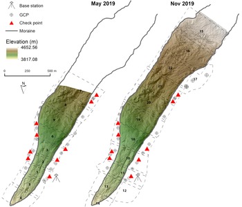
Annapurna III Glacier was surveyed by UAS twice, first on 16–17 May 2019 and later on 20–21 November 2019, encompassing most of the ablation season. Images were collected using a rotary-wing UAS (Mavic 2 Pro from DJI) fitted with a GPS/GNSS satellite-positioning system and a 20 megapixel Hasselblad camera (i.e. 5472 by 3648 pixels) that captures JPEG images (DJI, 2019) (Table S1). Map Pilot for DJI app was used to pre-program mission parameters which were uploaded to the UAS autopilot to fly a grid pattern at a constant elevation (with respect to ground) using the ‘terrain follow’ feature (Map Pilot, Reference Map Pilot2017). The imagery acquisition constituted nine flights in May 2019 and 13 flights in November 2019. In November 2019, we had greater success recharging batteries, enabling more flights and greater coverage of the glacier, thus also reaching higher elevations (Fig. 2). For all flights, the average flight altitude was set to 90 m above ground, the forward image overlap to 80%, the side overlap to 75%, and flight speed to 4 m s−1 (Table S2).
Overview of the surveyed area, check points and GCP locations for May and November 2019 missions at Annapurna III Glacier.

2.3 GNSS base station and ground control points
In May 2019, before the UAS data collection, 27 ground control points (GCPs) were established and surveyed using a differential GPS setup (Fig. 2). These GCPs were strategically placed along the lateral moraines of the Annapurna III Glacier. The GCPs were created using white or red color painted circular targets on sufficiently large and stable rocks and were utilized for georectification of the photogrammetric point cloud and as check points for accuracy assessment. In November 2019, besides surveying the GCPs established in May, four more GCPs were added in the higher elevation reaches along the western moraine of the glacier. The targets were distributed fairly evenly across the mapped area. However, reaching the higher elevation of the study area (with steep slopes and in proximity to the icefall) was extremely difficult and targets could not be established there (Fig. 2).
In both May and November missions, a Trimble Net R5 base with Zypher Geodetic antenna was installed on a tripod near the western lateral moraine in proximity to the camping site (Fig. 3a). This base station was configured to collect data every 10 s for a 15-h period (i.e. entire duration of the rover data collection). Two Trimble GeoXH 6000 units were used as dGPS rovers (Fig. 3b). To avoid error due to changes in antenna pole inclination, GCPs were sampled every second for a duration of 1-min. These datasets were later post-processed with Trimble Pathfinder (Trimble, 2000).
(a) A differential GNSS base station (location shown in Fig. 2), (b) the GNNS rover collecting data over a marked GCP and (c) the utilized quadcopter UAS.

2.4 SfM processing-point cloud, DSM and orthomosaic generation
The images collected during May and November were analyzed to generate 3-D point clouds and 2-D DSMs and orthomosaics of the Annapurna III Glacier and surrounding area following structure-from-motion (SfM) workflows (Westoby and others, Reference Westoby, Brasington, Glasser, Hambrey and Reynolds2012; Lucieer and others, Reference Lucieer, Jong and Turner2014). We performed an SfM analysis in Pix4Dmapper Pro software. Specific details of algorithms implemented in the Pix4D package are not available due to the proprietary nature of the software but some details regarding the parameters utilized within the software can be found in Pix4D (2019) (Table S3).
2.5 Accuracy assessment
The accuracy of the DSMs was assessed in multiple ways. First, the SfM processing provided horizontal and vertical residuals (i.e. the differences between actual and estimated coordinates during the bundle adjustment) for the 18 GCPs (Supplementary Table 3). Error is provided as mean and sigma of x–y–z differences, which describes how well the point cloud fits the in-scene ground targets. Second, the horizontal and vertical residuals calculated by overlaying nine independent validation check points and comparing them against the x–y–z values extracted from DSM surface provide a less biased and more precise error estimate. Third, the vertical uncertainty was also evaluated by calculating differences between the May and November DSMs for off-glacier terrain areas that were not subject to any change during the study period.
2.6 Glacier flow corrections
To derive changes in glacier mass balance from a pair of DSMs, it is necessary to correct for the horizontal velocity (us), the vertical velocity (ws) and the angle of the glacier surface tangent (α), all of which contribute to the apparent thinning pattern (Hooke, Reference Hooke2019). To estimate the horizontal displacement between May and November, we employed automated feature tracking. Both DSMs were resampled to 1 m and were used to produce multidirectional hillshades which were analyzed using orientation correlation with the ImGraft toolbox (Messerli and Grinsted, Reference Messerli and Grinsted2015). The displacement result was cleaned by eliminating values with low-correlation scores (<0.5), low signal-to-noise ratio (<2) or exceptionally high displacement (>8 m). This filtering resulted in displacement maps with some gaps (10% of the survey area) mostly near ice cliffs, which we filled using cubic spline interpolation. We assessed the uncertainty of the measured displacements as the normalized median absolute deviation of the x- and y-components of off-glacier measured displacement, combined in quadrature.
The cleaned displacement dataset was used to perform the horizontal flow correction by back-warping the November 2019 DSM to the corresponding May positions (Brun and others, Reference Brun2018). We additionally perform a vertical correction to account for downslope movement following Brun and others (Reference Brun2018): we applied a 900 m Gaussian filter to the ASTER GDEMv3 (NASA/METI/AIST/Japan Spacesystems, 2019), then used the measured displacements to determine the vertical component of downslope flow.
For any glacier, the net ablation is partially compensated by the emergence velocity, which refers to the upward or downward flow of ice relative to the glacier surface (Cuffey and Paterson, Reference Cuffey and Paterson2010; Hooke, Reference Hooke2019). To estimate the emergence over our study period, we used a flux gate approach similar to Vincent and others (Reference Vincent2016), Brun and others (Reference Brun2018) and Miles and others (Reference Miles2018). We identified a flux gate across the upper boundary of the surveyed area and calculated the flux of ice through this cross-section into the lower glacier. Due to the lack of in situ ice thickness data, we utilized the multi-model consensus ice thickness estimate and its standard error from Farinotti and others (Reference Farinotti2019), and the surface displacements derived from ImGraft analysis.
We bilinearly interpolated the ice thickness and surface displacement grids at 10 m interval along the flux gate, then determined the surface displacement component perpendicular to the flux gate. As the importance of basal sliding is unknown for this glacier, we nominally assumed that basal sliding accounts for 50% of the surface motion and considered the full range [0%, 100%] in our uncertainty estimate. We then integrated the flow equation with an assumption of simple sheer to calculate column-averaged displacement along the flux gate (Huss and others, Reference Huss, Sugiyama, Bauder and Funk2007). The total flux through the cross-section was then calculated as the integral of the product of ice thickness and column-averaged displacement along the flux gate. Finally, we calculated the mean down-glacier emergence velocity $( {\overline {w_{\rm e}} } )$ by dividing this by the glacier area below the flux gate.
2.7 Comparison between May and November point clouds and DSMs
We initially derived the pattern of elevation changes for the overlapping survey area from DSM differencing (without flow correction) by creating a DSM of difference (DoD) (i.e. negative values indicate elevation lowing or ice loss from May to November). This pre-flow correction DoD was used to derive mean elevation change and volume change. We estimated the uncertainty on elevation difference between the two DSMs, ɛ Δh, according to McNabb and others (Reference McNabb, Nuth, Kääb and Girod2019), following equation:

where ɛ rand and ɛ bias are, respectively, the std dev. and median of elevation changes over stable ground, n is the number of pixels falling into the glacier outline, L is the autocorrelation distance and r is the pixel size. The calculated uncertainty value for the entire domain was ±0.18 m. Using the vertical errors associated with the May and November DSMs (i.e. ±11 cm and ±16 cm vertical RMSE respectively), we also calculated a minimum level of detection (minLoD) value (as the sum of individual DSM errors in quadrature) which was very similar to the uncertainty value calculated earlier (±0.19 m).
The elevation difference values calculated above includes effects of glacier flow. In order to determine volume change solely related to net ablation, we first deformed the November point cloud by displacing individual points to account for the 3-D glacier flow during the study period, as described above for the raster data above. The flow-corrected point clouds from May and November were then gridded to generate DSMs at 0.1 m pixel resolution, which were differenced to determine mean volume melted/ablated which was used to determine the mean elevation change and total volume change over the period. Results are reported as volumetric and aerial changes per-pixel and for the entire monitored area of the Annapurna III Glacier.
The flow-corrected DoD represents the planimetric net mass balance over the survey area, but due to the rugged debris-covered glacier topography, this does not correspond to melt, which happens in the surface-perpendicular direction. To quantify ice melt distances, we performed point cloud differencing using the M3C2 method (Lague and others, Reference Lague, Brodu and Leroux2013). Unlike DSM differencing which calculates changes in the vertical direction, the M3C2 algorithm first selects a set of points (also called ‘core points’) on which it computes best-fitting normal direction and the changes between point clouds are calculated along this surface normal direction (as depicted in Fig. 9). The propagated RMSE calculated as the quadrature of two UAS surveys was used as the registration error in the point cloud differencing analysis. The M3C2 output includes a point cloud containing M3C2 distance, significant change and distance uncertainty. Distance uncertainty is given as the confidence interval, also called level of detection (LOD) given as:

where σ 1 and σ 2 represent that roughness of individual point cloud in subset of clouds of diameter d and size of n 1 and n 2 and reg is the registration error. The distribution of registration error is expected to be spatially uniform and isotropic (Lague and others, Reference Lague, Brodu and Leroux2013). If the |M3C2 distance| > C95% the significance value is 1 or otherwise 0. The significance values were used to select only the significant M3C2 values on which mean and std dev. were calculated. The point cloud of significant M3C2 distance values were gridded and analyzed to better understand their distribution considering elevation and slope for the entire monitored area of the glacier. The M3C2 raster was also filtered to select ice cliff areas that were debris-free in both May and November. These selected M3C2 values were analyzed to quantify the debris-free ice-cliff melt rate and the influence associated driving factors (e.g. aspect) on melt rate. Although DSM differencing provides correct total volumetric changes, it may not correctly reflect melt distance. On the other hand, M3C2 directly accounts for topography, but thusly-derived melt distances are not suitable for using with planimetric areas. Therefore, we utilized the slope values and planimetric area of each pixel to derive the actual surface area (Jenness, Reference Jenness2004) and then calculated the melt volume based on M3C2 distance values and compared the same with the DSM differencing derived volume change.
2.8 Analysis and interpretation
In addition to reporting the mean volumetric change and melt distances for the entire Annapurna III Glacier survey area, we examined and interpreted glacier surface changes within four domains that experienced interesting patterns of melt. We then examined the glacier-wide relationships of surface elevation and slope to melt distances to consider the role that surface topography plays in promoting melt heterogeneity across the glacier surface. Considering the range of ice cliff changes exhibited at Annapurna III Glacier, we performed assessment of ice cliff and non-ice cliff melt across the entire survey area by first individually interpreting ice cliffs in both May and November. Furthermore, we determined ice cliff extent at two levels of confidence: at high confidence level, areas that were identified as ice cliffs in both May and November surveys were selected (i.e. intersection of both surveys). At slightly lower confidence, we selected areas that were identified as ice cliffs in either of the surveys (i.e. union of both surveys) while the remaining monitored area was categorized as non-ice cliff area (Fig. S4). This approach allowed us to show how the interpreted cliff area impacted the attributed melt. Finally, we leveraged our high-quality results to quantify the aspect-dependence of ice cliff melt rates.
3. Results
3.1 GNSS and DSM accuracy
The coordinates of the dGPS base station were positioned with an estimated (vertical + horizontal) uncertainty of 0.046 m during May 2019 and 0.066 m during the November 2019 campaign. After post-processing the GCPs and check points with Trimble Pathfinder Office, their positional errors were estimated to be under 0.03 m (May 2019) and 0.039 m (Nov 2019). Combining these sources of error in quadrature, the maximum expected positional error for the two surveys was 0.069 m. We then assessed the accuracy of the DSMs based on the residuals of the GCPs. The distribution of the GCP residual for May 2019 shows that the DSM had accuracy within 0.20 m for both vertical and horizontal directions. For the November 2019 DSM, the errors were within 0.30 m, but error was <0.15 m for the majority of the measurements (Fig. 4).
Histograms of differences (errors) between check points and GCP surveyed elevations and DSM elevation for May 2019 and November 2019. (a) May 2019 check points, (b) November 2019 check points, (c) May 2019 GCPs and (d) November 2019 GCPs and (e) histogram of elevation differences for the off-glacier area shown in Fig. 1.

The error statistic provided above tends to overestimate model accuracy. SfM processing in its various stages (i.e. aligning images and orthorectification) introduces some error. DSM accuracy should therefore be evaluated by comparing survey points not used in model generation (i.e. check points) and comparing DSM difference over the off-glacier area that is expected to experience no vertical change. Comparison of the May 2019 DSM with independent check points showed a mean difference of −0.001 m with a std dev. of 0.119 m (Fig. 4). For November 2019 DSM, the mean difference to check points was −0.04 m with a std dev. of 0.109 m (Fig. 4). The average deviation between the two DSMs when compared for off-glacier area (outlined in Fig. 1) was 0.01 ± 0.13 m (Fig. 4e). This result highlights that the point clouds and DSMs used in the following analyses were aligned accurately.
3.2 Glacier flow
During May–November 2019, the horizontal displacement of the glacier ranged from 5.9 m in the upper part to negligible (completely stationary) near the lateral moraines on both sides and the glacier snout (Fig. 5). The glacier exhibited higher rates of motion above the 4160 m contour (4.5–5 m over the study period), and lower rates of motion below this (3–3.5 m). At ~4160 m, there is a sudden break in slope, with lower surface gradient (<25°) at lower elevations relative to the higher elevations (>35°). The off-glacier displacements we measured were exceedingly small, resulting in a displacement uncertainty of just 0.1 m over the study period.
Horizontal displacement (m) derived at 4 m spacing from orientation correlation analysis of 1 m hillshade using the ImGraft toolbox.

Along the 650 m flux gate, we estimated a mean ice thickness of 26.5 ± 5.3 m and a mean depth-averaged displacement of 3.8 ± 0.42 m. We therefore estimated the total volumetric flux of ice through the flux gate as 55 100 ± 12 400 m3 for our survey interval, leading to a mean emergence of 0.18 ± 0.03 m for the entire domain during this period. We note that this calculation did not determine the spatial variability of emergence velocity across our study domain, so we expect localized errors in the pattern of mass balance.
3.3 Glacier elevation changes and melt distances
The pattern of surface elevation changes from DSM differencing was highly heterogeneous across the glacier area, with a mean elevation change of −1.1 ± 0.18 m and a std dev. of 0.94 m, equivalent to a loss of 308 053 m3 of glacier volume (Table 1). Following flow corrections, the change pattern was largely coherent, revealing more clearly the surveyed area's pattern of mass change during the observed ablation season. The maximum magnitude of elevation change was −10.33 m and the maximum surface raising was +2.62 m, but the vast majority (~96%) of the values were within −2.57 to +0.38 m (Supplementary Fig. 2).
Comparison of DSM differencing and point cloud differencing derived estimates

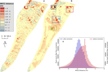
Results from the M3C2 analysis of both before and after flow correction of point clouds are shown in Fig. 6 and a visual comparison of elevation difference (DH) before and after flow correction in Fig. S5. The banding pattern of crests and troughs that is visible in the uncorrected results disappeared when flow-corrected point clouds are used for M3C2 analysis, confirming the success of the flow correction. The figure also highlights the spatial variability of melt over the monitored area, which is additionally summarized as a histogram in Figure 6b. More than 80% of flow-corrected points had statistically significant M3C2 distance values. These points with significant M3C2 distance had a mean melt distance of −0.87 m and a std dev. of ±0.79 m. The mean melt rate, calculated as the slope weighted mean of M3C2 distances divided by the survey interval, was −0.47 cm w.e. d−1. No significant change was observed for the debris in the periglacial area, confirming the accurate alignment of the two point clouds.
Results of point cloud differencing where M3C2 distance is presented as gridded raster, (A) before flow correction and (B) after flow correction, also showing a histogram of M3C2 distances before and after correction. Panels (a), (b), (c) and (d) highlighted in (B) are referred to and shown in detail in next figures.

The difference between DSM differencing and M3C2 distance is conceptually shown in Fig. 8 which focuses on one of the ice cliff systems (box ‘a’ in Fig. 6b). The changes along a transect illustrate the fact that traditional DSM differencing calculates changes in elevation along the vertical direction (Fig. 7d) while the M3C2 method calculates changes normal to the local surface (Fig. 7e).
(a) and (b) represent DSM difference and gridded M3C2 for a selected ice cliff highlighted in area of interest ‘a’ of Fig. 7a; (c) shows the absolute difference between the two; (d–f) depict the conceptual difference between DSM differencing vs M3C2 distance by plotting the cross-section for the transect shown in (a) and (f) shows the comparison of derived elevation changes from DSM differencing and M3C2 distance for the transect.

Comparison of results over the entire domain showed that mean melt distance (−0.87 m) was lower than mean thinning value (−1.1 m) due to steep sloping areas, often by 15–20% (values above) as aggregated difference. Yet, the calculated volume changes from both methods largely agree (due to large overlap of uncertainty) (Table 1). Although ice cliff melt rate was much higher than non-ice cliff areas, the melt rate of ice cliff varied a lot based on the definition of ice cliff (i.e. −3.9 m for ice cliff intersection-of-areas vs −2.8 m for union-of-areas). The union-of-areas significantly dilutes the ice cliff melt rates for both DSM and M3C2 approaches (30–40% decrease) due to marginal effects integrating both cliff and non-cliff time periods (Table 1).
3.4 Melt patterns and associated processes for selected areas
Here, we examine and interpret the four selected domains of topographic change depicted in Fig. 6b.
3.4.1 Domain ‘a’
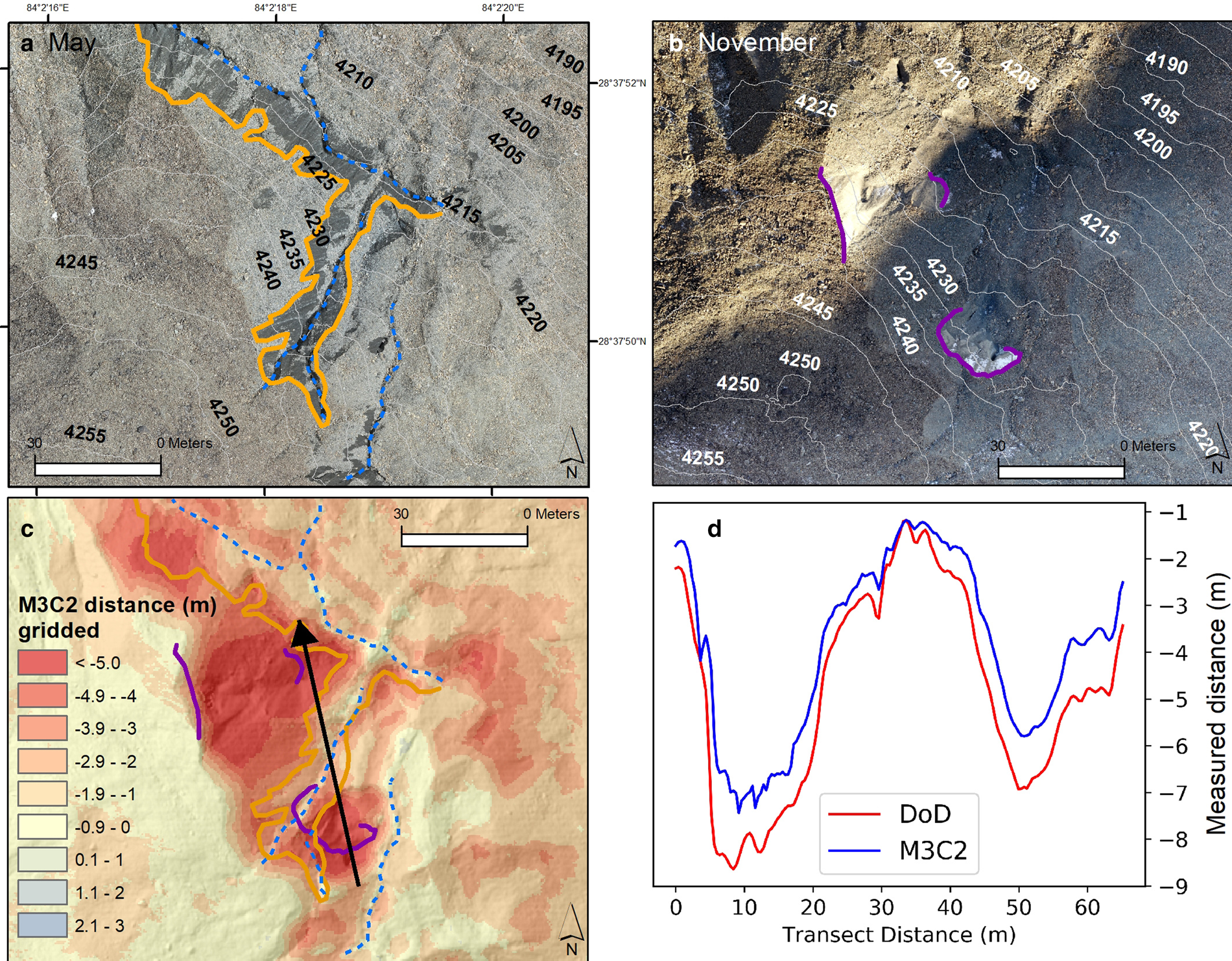
In May 2019, domain ‘a’ contained three ice cliffs of varying orientations surrounding a surface depression containing a small supraglacial pond (Fig. 8a). By November 2019, this domain experienced considerable changes, with ice cliffs melting up to 8 m perpendicular to their surface and retreating into areas that are more shaded. The changes experienced by individual ice cliffs were not uniform during this study period, although. The cliff-oriented southwest experienced a dramatic reduction in exposed ice area accompanied by melt distances of up to 7 m. The north-facing ice cliff experienced a slight rotation and also shrank in area, but only experienced melt of 2.5–3.5 m during the study interval. The third ice cliff faced NNE in both surveys and showed the smallest change in surface area between May and November. Although it split into two distinct ice cliffs by November, both areas experienced melt distances broadly exceeding 5 m during the survey interval. By November, the May supraglacial pond was no longer apparent, but another small pond had formed near the supraglacial conduits visible in May.
Changes in surface features around a selected ice cliff highlighted in area of interest ‘a’ of Fig. 6b. (a) and (b) shows the perspective view of dense point clouds of May and November 2019 respectively, where annotations include ice cliffs, supraglacial pond, englacial conduits and aspect of ice cliffs; (c) shows respective M3C2 distances.

The aspect-dependent behavior of ice cliff surface melt (Buri and Pellicciotti, Reference Buri and Pellicciotti2018; Steiner and others, Reference Steiner, Buri, Miles, Ragettli and Pellicciotti2019) is evident in this domain: the north-facing ice cliffs steepened during the study interval (regardless of area change) whereas the south-facing cliff shallowed in slope and shrank (Fig. 8). The result is that the highest apparent melt distance occurs for the large cliff oriented NNE: this feature stably backwasted for the study period, whereas the south-facing cliff may have melted quickly, but was also progressively reburied by debris before November, reducing the overall melt distance.
It is apparent that there was considerable debris mobilization at this site during the study period, which is manifest as a progressive downslope increase in elevation change (more positive lower), as reported by Westoby and others (Reference Westoby2020). We observed elevation increases of up to 0.5 m at the bottom of this depression, similar to the observations by Thompson and others (Reference Thompson, Benn, Mertes and Luckman2016) at Ngozumpa Glacier. Although the amount of elevation increase (0.5 m) is close to the uncertainty level, the pattern of topographic changes suggests this was in part due to debris accumulation.
3.4.2 Domain ‘b’
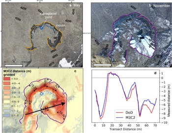
In May 2019, domain ‘b’ was occupied by a nearly circular ice cliff following a supraglacial stream segment originating in a small supraglacial pond and draining into an englacial conduit (Fig. 9a). By November 2019, this ice cliff maintained its general shape, but had spread radially and grown in overall area. The greatest cliff expansion occurred near the May 2019 moulin location, while the supraglacial stream and pond were no longer evident in November 2019. Slope-perpendicular melt distances reached 9 m near the position of the May cliff crest, and most of the combined May and November cliff area experienced slope-perpendicular melt of 4 m or more. A 2-D profile (Fig. 9d) highlights the spatial variability of topographic change: both the DoD and M3C2 measurements identify the reduction in melt for the area of the cliff which developed debris cover during the study interval as well as the elevation increase over part of the non-cliff domain.
Changes in surface features around area of interest ‘b’ shown in Fig. 6b. (a) and (b) orthomosaics of May and November, (c) gridded M3C2 distance and (d) comparison of DSM differencing (DoD) and M3C2 values along the shown transect.

At this site, the ice cliff expansion was likely driven by debris evacuation and thermal undercutting by the supraglacial stream, which, given the high melt distance in the vicinity of the moulin, we interpret was active during the monsoon. Although the apparent elevation increases surrounding the ice cliff were generally 1 m, we do not expect that this is attributable to debris thickening. This elevation increase was also broadly apparent surrounding domain ‘b’ and was not related to the local topography as in domain ‘a’ or prior studies. As this area also experienced the highest rate of glacier flow within the survey area, we expect that these elevation increases were primarily due to emergence rates locally higher than the average value we used in our flow correction.
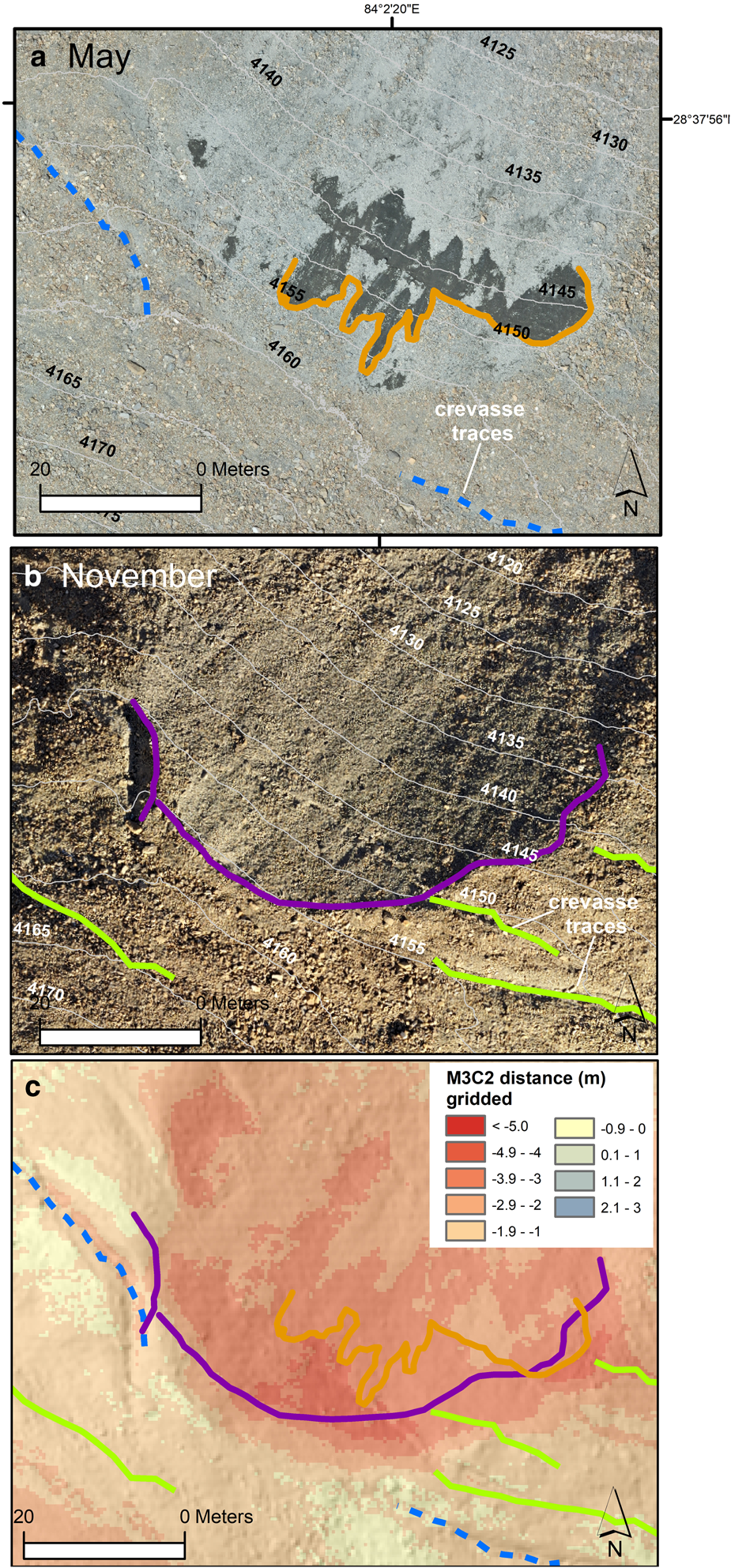
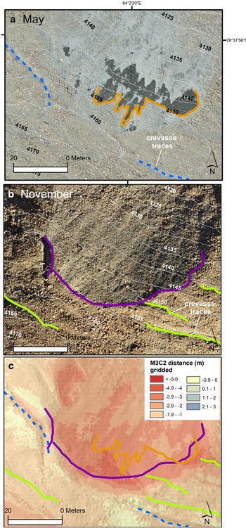
3.4.3 Domain ‘c’
In domain ‘c’, May imagery showed the presence of two very linear supraglacial stream channels bordered by ice cliffs (Fig. 10). These stream channels appeared to have formed along crevasse traces, while a set of relict drainage conduits or stream channels apparently crossed this active drainage network. In November, no sign of the crevasse traces or active supraglacial drainage network was visible, while the ice cliffs had generally reduced in area. This site showed melt distances of 7 m over a large area that, unlike domains ‘a’ and ‘b’, did not clearly correspond to the ice cliff areas in May or November. Lacking subseasonal observations, we cannot conclusively interpret the driver of the high melt rate here, but it is possible that this area was occupied by an ice cliff for much of the study interval before eventual reburial. However, the steep slope of this high-melt area would have promoted debris mobilization (Moore, Reference Moore2018), so it is also possible that this area simply exhibits thinner debris; the complete reburial of the crevasse traces and supraglacial network is also indicative of rapid debris mobilization.
3.4.4 Domain ‘d’
Domain ‘d’ was an area of dramatic surface change (Fig. 11) that was not obvious from the point cloud differencing before the flow-correction (Fig. 6a). In this area, a patchy ice cliff was evident in May 2019, but had disappeared entirely by November. This ice cliff occupied a shallow surface recession, which had moderate surface slopes (20–25°) and a lighter, grayer debris appearance than its surrounds in the May orthomosaic, characteristic of recent debris reworking. This area experienced moderately higher melt distances (>2 m) than the survey area average (0.85 m), suggestive of thinner debris coverage. We also note that surrounding this recessed area are several linear surface features running perpendicular to the surface slope and the direction of glacier flow, which we interpret as buried crevasses; these features also correspond to higher M3C2 distances.
Taking these distinct features into account, we hypothesize that the ice cliff observed in May originated as an opening crevasse, which evacuate debris and can lead to ice exposure (Moore, Reference Moore2018). We expect that the resulting cliff produced the local surface recession as the result of backwasting over several years. The final stage of cliff reburial occurred during our study interval as the cliff exhausted the available topography, as suggested in Brun and others (Reference Brun2016). It is apparent, however, that the reworking of the debris surface by the cliff's backwasting led to thinner debris over a broad area (Bartlett and others, Reference Bartlett, Ng and Rowan2020). We note that the melt distance of the area occupied by the ice cliff in May was 3–3.6 m, whereas the peak melt distances (>4.5 m) occurred in an area not observed to be occupied by an ice cliff, and melt distances within the scallop area (>3 m) were twice the value of the surrounding area (1–1.9 m). Thus, if our interpretation is correct, this cliff's life cycle enhanced melt even in locations and for periods when it is not itself present.
3.5 Topographic dependence of melt distances
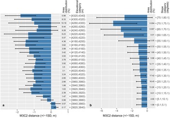
The melt distance results showed considerable spatial variability, so we initially examined the relationship between topographic parameters and melt distances. Our results show no systematic relationship between mean melt distances and elevation (Fig. 12a). A mass-balance inversion has been reported previously for debris-covered glaciers due to the increasing debris thickness nearing glacier termini (Benn and Lehmkuhl, Reference Benn and Lehmkuhl2000; Anderson and others, Reference Anderson, Anderson, Armstrong, Rossi and Crump2018; Bisset and others, Reference Bisset2020). Our field investigations of Annapurna III unfortunately did not include measurements of debris thickness, but the measurements of Heimsath and McGlynn (Reference Heimsath and McGlynn2008) show debris thickness increasing from ~0.4 m near the top of our survey domain to >2 m at the glacier terminus. Considering the relative melt reduction that is generally expected under 0.4 m of debris (e.g. Nicholson and Benn, Reference Nicholson and Benn2006), and our spatially-distributed melt distance results (Fig. 7), it is clear that the altitudinal variability of melt rates at this site is not due to the altitudinal variability of debris thickness, but to the distribution of ice cliffs. For example, the highest-altitude band (>4320 m) clearly has the greatest melt distance (−1.79 m) due to the prevalence of ice cliffs in this domain, which also leads to the highest variability in in M3C2 distances. This bears out in the variability of M3C2 distances within each elevation band, which overwhelm any altitudinal pattern. We note that the lowest elevation areas occupied by the glacier (i.e. glacier snout and adjoin glacier reaches) show a slightly positive M3C2 distance, indicating elevation gain of 0.24 m. These results are approximately at the level of uncertainty, but we also note that seasonally enhanced ice velocity (Kraaijenbrink and others, Reference Kraaijenbrink2016) can lead to slight terminus advances during the monsoon even for a nearly-stagnant glacier losing mass; consequently this area may experience a higher ice emergence rate than the domain's mean value. Overall, the pattern indicates that despite an elevation range of 500 m and debris thicknesses varying at the meter-scale (Heimsath and McGlynn, Reference Heimsath and McGlynn2008), the spatial variability of melt across the surveyed area of Annapurna III Glacier is primarily controlled by the spatial distribution of ice cliffs.
Distribution of M3C2 distance (a) calculated by 20 m elevation bands and (b) 5° slope class. In each figure, the bars indicate mean with ±1 std dev. and percent value on the y-axis denotes the distribution of terrain in each bin.

The distribution of melt distance was therefore also slope dependent. For glacier areas with <25° slope, melt distances were uniformly low, with a mean <1 m and std dev. of 0.7 m (Fig. 12b). Areas with slope between 25° and 55° showed slightly higher melt distance (~1 m) but with a consistent increase in spatial variability with increasing slope. Prior studies have identified ice cliffs as areas with steep slopes, usually >40° (e.g. Reid and Brock, Reference Reid and Brock2014; Herreid and Pellicciotti, Reference Herreid and Pellicciotti2018) but Annapurna III Glacier exhibits little enhancement to melt distances until slopes reach 55°. Indeed, the heterogeneity of melt distances for slopes above this threshold, which is evidenced in the focused domains, suggests that debris patches on otherwise-steep cliff surfaces can sometimes play a significant local role in reducing melt locally, as suggested in Herreid and Pellicciotti (Reference Herreid and Pellicciotti2018). Finally, it is clear that areas with >55° slope showed significantly higher melt distances, and variability, with mean melt distances 2–4 times that of areas below 55° slope.
4. Discussion
4.1 The relative merits of M3C2 and DH melt measurements
DSM differencing has been widely utilized in previous studies (Immerzeel and others, Reference Immerzeel2014; Thompson and others, Reference Thompson, Benn, Mertes and Luckman2016; King and others, Reference King, Turner, Quincey and Carrivick2020), as it provides a direct and efficient approach to assess the elevation change (DH) over a surface. However, our results show the limitations of this approach for monitoring areas of rugged surface topography. For areas with gentle slope (<10°) that do not undergo high magnitude of change, DSM differencing derived elevation difference (DH) closely matches the M3C2 derived melt distance, with distance differences <0.5 m (e.g. Figs 7, 9d, 10d). However, in areas with relatively higher slope (>20°) that experience higher magnitudes of change (e.g. ice cliff backwasting), the difference is considerable as DSM differencing tends to overestimate change by at least 1 m. Consequently, we advocate the use of the M3C2 method (after flow correction) to supplement traditional geodetic measurements of volume change with distributed measurements of slope-perpendicular melt rates. These new measurements open the possibility to disentangle and quantify the mechanisms controlling elevation change in 3-D. Such measurements extend beyond net volume change or average rate assessments (Brun and others, Reference Brun2016) are highly valuable for calibration and evaluation of numerical models (e.g. Buri and others, Reference Buri, Pellicciotti, Steiner, Miles and Immerzeel2016). Our results demonstrate that this is also relevant for debris-covered areas, where surface slopes are often >20° (Fig. 13), leading to possible mismatch between even flow-corrected DH and manual measurements.
(a) Distribution of sampled M3C2 distances for cliff and off-cliff glacier areas, showing mean melt distances with dashed lines, and (b) distribution of local surface slopes for cliff and non-cliff areas.

4.2 Ice cliff melt at Annapurna III Glacier
The melt enhancement of ice cliffs has been a topic of focused research (Sakai and others, Reference Sakai, Nakawo and Fujita2002; Immerzeel and others, Reference Immerzeel2014; Brun and others, Reference Brun2018) since these features can account for a considerable portion of debris-covered glaciers' total mass loss (Pellicciotti and others, Reference Pellicciotti2015; Thompson and others, Reference Thompson, Benn, Mertes and Luckman2016). Indeed, at Annapurna III Glacier these features also exhibited the greatest melt distances. However, unlike previous studies, our highly detailed results show considerable changes in cliff areas over even the short survey interval. We first determined areas that were cliff in both surveys and areas that were not cliff in either survey (Supplementary Fig. 1), and determined the mean M3C2 melt distances for these two domains (Fig. 13). Our results indicated that ice cliffs had significantly higher melt distances (mean −2.9 m, std dev. 1.5 m) compared to debris-covered non-cliff areas (mean −0.75 m, ±0.53 m). This equates to an ice cliff enhancement factor of 3.9 relative to subdebris melt at Annapurna III Glacier, which is slightly higher than that reported for Changri Nup Glacier (Brun and others, Reference Brun2018) but considerably less than values reported for Lirung Glacier (Sakai and others, Reference Sakai, Nakawo and Fujita2002; Immerzeel and others, Reference Immerzeel2014). Across the whole domain and considering both surveys, ice cliffs affected 5.1% of the monitored area (union of cliff areas in May and November) and covered 3.78% of the monitored area on average, but directly contributed 11% of the total melt generated from the monitored area.
However, the sampled ice cliff areas show considerable variability in melt distances. Past studies have suggested that ice cliff aspect can control the distribution of radiative fluxes and thus cliff evolution (Sakai and others, Reference Sakai, Nakawo and Fujita2002; Buri and Pellicciotti, Reference Buri and Pellicciotti2018), and our melt distance results also show a relationship between ice cliff melt and aspect (Fig. 14). Counterintuitively, north and northwest-facing ice cliffs showed highest melt distance (median −4.7 m), while the east and southeast-facing aspects experienced much lower melt distance (median −2.6 m). It is notable that the NW aspect cliffs were the only orientation to experience a low spread in melt distances (inter-quartile range 0.75 m), and in fact show the greatest value in the lower-bound of the melt distance distribution, suggesting that these cliffs were the least affected by debris reburial. Our results show the clearest observational evidence of this counterintuitive process to date.
Box plots of ice cliff melt distance for different aspects on Annapurna III Glacier. The vertical line represents the mean melt distance for the entire sample of ice cliffs.

4.3 The challenge of attributing melt to ice cliffs
Our observations at Annapurna III indicate that ice cliff melt enhancement factors determined from remote sensing should be treated with caution. Our examination of focus areas (a)–(d) highlighted multiple confounding factors for determining ice cliff melt rates from even high-precision DSMs after flow correction, and highlights that topographic changes over an interval are often the result of complex local changes; only for clear, isolated features is the melt rate meaningful (e.g. Brun and others, Reference Brun2016). The combination of glacier flow corrections and M3C2 distance measurements provided the ability to measure melt distances directly, but the spatial attribution of that melt to ice cliffs remains challenging. An advantage of sub-meter resolution imagery from UAS platforms is that independent operators tend to reach close consensus with regards to cliff outlines (Brun and others, Reference Brun2018) which is not always the case for even meter-resolution satellite imagery (Kneib and others, Reference Kneib2021), but ice cliff outlines change over an interval due to backwasting (a lateral shift) but also due to cliff-marginal processes (Buri and others, Reference Buri, Pellicciotti, Steiner, Miles and Immerzeel2016). At both sites (a) and (b), ice cliff melt distances were very high, and the areas of greatest melt distance were clearly bounded by cliff outlines. At sites (c) and (d), however, broad patterns of enhanced melt are evident in direct association with ice cliffs, but outside the observed ice cliff extent. At these sites, multiple processes associated with ice cliffs (debris mobilization, conduit thermal erosion and ice cliff reburial), confound the melt signal. The spatial attribution problem has been dealt with in past efforts through triangulated irregular networks (Brun and others, Reference Brun2016, Reference Brun2018) or through localized M3C2 analyses (Watson and others, Reference Watson2017). However, these approaches still rely on cliff/non-cliff discrimination in the melt signal, and are best suited to well-defined features. For complex cliff geometry changes, the simpler alternative approach is to attribute the entire enhanced-melt area to ice cliffs, rather than that bounded by the cliff itself (Immerzeel and others, Reference Immerzeel2014; Thompson and others, Reference Thompson, Benn, Mertes and Luckman2016), leading to a higher melt portion attributable to cliffs. Our results show that the choice of distance measurement method (DSM difference vs M3C2 distance) and relevant domain (union or intersection of outlines) can produce substantial differences of ~20 and ~40%, respectively, in the melt rates attributed to cliffs, even after flow corrections (Table 1).
Underlying the spatial problem is the problem of temporal attribution. Two types of confounding subseasonal change are evident at Annapurna III: (1) instances of a cliff (or cliff segment) emerging or being reburied during the interval (leading to cliff observation at one side of the interval) and (2) the possibility of a cliff emerging and being reburied within the interval (no cliff observed). For the first case, rapid reburial or emergence of ice cliffs (e.g. subseasonal, as in at site ‘d’) leads to intermediate melt rates. This is evident at site ‘d’, where a cliff was reburied (Fig. 11), but is also apparent for south-facing ice cliffs (Fig. 14) which are more likely to be reburied rapidly (Buri and Pellicciotti, Reference Buri and Pellicciotti2018). Although possibility (2) cannot be observed directly over the interval, patterns of melt at Annapurna III and Changri Nup Glacier show localized melt enhancement within a well-defined boundary likely involving a combination of moisture availability, reduced debris thickness, debris mobilization and cliff appearance and reburial (Moore, Reference Moore2018; Westoby and others, Reference Westoby2020). The best way to resolve this attribution issue is with shorter observation intervals, which may be difficult to implement with a UAS platform at remote sites but could be accomplished with repeat satellite stereo acquisitions or time-lapse photogrammetry (Mallalieu and others, Reference Mallalieu, Carrivick, Quincey, Smith and James2017).
4.4 Limitations and opportunities for future research
The UAS surveys and processing workflow have been meticulously carried out in view to limit the uncertainty of the data processing, following established methods (James and Robson, Reference James and Robson2014; Smith and others, Reference Smith, Carrivick and Quincey2016; James and others, Reference James2019). However, a key limitation in this analysis is the method to estimate flux divergence at the site, which necessarily used modeled ice thickness to estimate ice flux into the survey area. This method has some precedent (e.g. Miles and others, Reference Miles2018, Reference Miles2021; Bisset and others, Reference Bisset2020), but is best constrained with in situ ice thickness measurements (Fujita and Nuimura, Reference Fujita and Nuimura2011; Vincent and others, Reference Vincent2016; Nuimura and others, Reference Nuimura, Fujita and Sakai2017; Wagnon and others, Reference Wagnon2020). In situ ice thickness observations remain scarce in the Himalaya and the performance of available ice thickness models for debris-covered glaciers has not been thoroughly established, so it is difficult to assess the ice thickness uncertainty, but new measurements are emerging that should help to constrain future models (Pritchard and others, Reference Pritchard2020).
To bound the flux divergence error, we consider Lirung Glacier as a reasonable analog to Annapurna III Glacier: they are similar in terms of accumulation mechanisms (avalanching and now-disconnected icefall), width (~500 m), and monsoon-period flow rates in the survey area (<10 m a−1). These attributes do not necessarily imply similar patterns of flux divergence, but may lead to a similar mean value in the glaciers' ablation area. The emergence velocities estimated for Lirung Glacier are on the order of 0.2 ± 0.1 m a−1 since 2000 (Immerzeel and others, Reference Immerzeel2014; Nuimura and others, Reference Nuimura, Fujita and Sakai2017), almost precisely our own estimate for Annapurna III in 2019. In an extreme case, considering a doubling of this value, the impact on our subsequent analysis and interpretations is negligible. Even with ice thickness transects, however, studies to date have only succeeded in assessing the mean flux divergence in a glacier segment, leading to spatial uncertainty regarding the corrected surface melt patterns. We do expect this to lead to melt underestimation at the uppermost portion of the survey area and overestimation below; however, this error has little influence on the local-scale contrasting melt patterns we observe at Annapurna III glacier.
Our results also highlight the need for additional observations to better quantify the glacier's melt patterns and controls. For example, seasonal and annual measurements of sub-debris ablation will be crucial to improve future distributed melt estimates and important to constrain numerical models, and the debris thickness measurements reported in Heimsath and McGlynn, (Reference Heimsath and McGlynn2008) should be expanded upon. In particular, the ice cliff and associated surface dynamics at the site are suggestive of monsoon debris mobilization, and subseasonal monitoring of monsoonal debris-covered glaciers would be useful to constrain the rates of debris motion and its influence on ice cliffs. In addition, we were able to survey an expanded domain of Annapurna III Glacier in November 2019 compared to May 2019. Given the upper debris-covered area's proximity to avalanche mass supply areas, it is likely to also exhibit higher rates of ice flow and lower debris thicknesses. Subsequent UAS and dGPS surveys should also target this larger area to quantify debris-covered glacier processes at the glacier-scale in this distinct and relatively accessible setting, adding perspective to the small set of Himalayan glaciers for which detailed measurements are available.
5. Conclusions
This study presents an application of DSM and 3-D point cloud differencing applied to repeated UAS survey data for detecting topographic change on the lower ablation area of Annapurna III Glacier. Our measurements provide the opportunity to explore debris-covered glacier melt patterns and processes at a new site, and highlight the heterogeneity of melt rates. Our results show that UAS-derived 3-D point cloud data provides a more suitable basis than elevation change for understanding the processes of debris-covered glacier melt. We show that ice cliffs are responsible for the slope dependence of melt rates and the inverted mass-balance gradient through the debris-covered area of this glacier, and confirm that north-facing cliffs experience higher overall melt rates than south-facing cliffs. Our results suggest that ice cliff melt at rates 3.9× that of subdebris melt, account for 11% of the survey area's melt, and dominate the spatial pattern of mass balance at this site. Ice cliff domain should be defined carefully to ensure that measurements actually represent ‘pure’ cliff as dilution can bias melt rate and enhancement factors. Careful and sophisticated measurement of ice cliff melt rate using M3C2 distance can provide more accurate estimate of ice cliff melt rate and enhancement factor. Our detailed examination of seasonal surface changes emphasizes that short-interval repeat surveys are necessary to disentangle the complex processes affecting ice cliff change and associated melt rates.
Supplementary material
The supplementary material for this article can be found at https://doi.org/10.1017/jog.2021.96
Acknowledgements
We are grateful for the constructive comments from Scientific Editor Neil Glasser and three anonymous reviewers, which greatly improved this manuscript. The authors thank the Home Ministry, Civil Aviation Authority and the Annapurna Conservation Area Project (ACAP) of Nepal for allowing UAS data collection; ACAP officials and Tashi Gale for guidance and logistical support in the field and Colin Belby for making the dGPS available. The first author thanks Bharat Babu Shrestha, Jackson Radenz, Kyle Zerbian, Aaron Christensen, Tejab Pun and David Holmes for participating in data collection missions and Planet Labs for providing imagery of the Annapurna III Glacier via their education and research program. The first author was partially funded through Faculty Research Grant from UW-La Crosse, and students were funded by Research and Creativity grant and Travel and Supplies Grant from the College of Science and Health at UW-La Crosse.


 Open access