


1. Introduction
In global fixed income markets, bond yields serve as barometers of economic conditions, offering insights into risk assessment, valuation, and investment strategy. In the insurance sector, interest rates are crucial for pricing and managing products such as life insurance (Gaillardetz, Reference Gaillardetz2008; Bernard et al., Reference Bernard, Le Courtois and Quittard-Pinon2005), annuities (Fontana & Rotondi, Reference Fontana and Rotondi2023; Günther & Hieber, Reference Günther and Hieber2024), and optimal investment strategies (Han & Hung, Reference Han and Hung2017; Wang & Li, Reference Wang and Li2018; Peng & Li, Reference Peng and Li2023). A persistent challenge is the phenomenon of yield curve inversion – where short-term yields exceed long-term yields – often signaling economic recession. Understanding the determinants of such adverse yield movements is vital for informed policy and portfolio decisions.
Research on the term structure of interest rates has evolved substantially over the past decades, following two main modeling paradigms. The first is the family of no-arbitrage models, such as Hull and White (Reference Hull and White1990) and Heath et al. (Reference Heath, Jarrow and Morton1992), which ensure consistency with market prices through dynamic arbitrage-free frameworks. The second comprises equilibrium term structure models, including those of Vasicek (Reference Vasicek1977), Cox et al. (Reference Cox, Ingersoll and Ross1985), and Duffie and Kan (Reference Duffie and Kan1996), which derive interest rate dynamics from economic fundamentals. A detailed overview of these models is provided in Cairns (Reference Cairns2004).
Whilst these models were typically derived based on continuous time stochastic diffusion models (s.d.e’s), there were, in parallel, classes of models developed in discrete time econometrics settings. Such approaches formulate term structure dynamics via state-space modeling and regression methods. Dobbie and Wilkie (Reference Dobbie and Wilkie1978) introduced an exponential model representing yields as a sum of two exponentials, a framework that became widely used in fixed income markets. Nelson and Siegel (Reference Nelson and Siegel1987) proposed the parsimonious Nelson–Siegel model, capturing the level, slope, and curvature of the yield curve. Svensson (Reference Svensson1994) extended it by adding a fourth term for greater flexibility, while Cairns (Reference Cairns1998) refined these models with additional exponential terms to mitigate instability issues noted in Dobbie and Wilkie (Reference Dobbie and Wilkie1978) and Svensson (Reference Svensson1994). These extensions were applied to the UK and German bond markets in Cairns (Reference Cairns1998) and Cairns and Pritchard (Reference Cairns and Pritchard2001), respectively.
Diebold and Li (Reference Diebold and Li2006) introduced autoregressive dynamics into the Nelson–Siegel model, improving long-horizon forecasts of US Treasury yields. Subsequent studies linked macroeconomic variables – capacity utilization, the federal funds rate, and inflation – to yield curve factors (Diebold et al., Reference Diebold, Rudebusch and Aruoba2006), and extended the model to a global multi-economy setting (Diebold et al., Reference Diebold, Li and Yue2008). Further developments included time-varying loadings and GARCH errors (Koopman et al., Reference Koopman, Mallee and Van der Wel2010), applications to corporate yields (Yu & Zivot, Reference Yu and Zivot2011), and assessments of parameter stability (Wahlstrøm et al., Reference Wahlstrøm, Paraschiv and Schürle2022).
Recent advances include quantile-based modeling for economic shocks (Iacopini et al., Reference Iacopini, Poon, Rossini and Zhu2024), arbitrage-free formulations (Eghbalzadeh et al., Reference Eghbalzadeh, Godin and Gaillardetz2024; Fontana et al., Reference Fontana, Lanaro and Murgoci2025), and stochastic process approaches for bond portfolios (Andersson & Lagerås, Reference Andersson and Lagerås2013). Comparisons with affine models are discussed in Filipovic (Reference Filipovic1999), while comprehensive reviews are provided in Diebold and Rudebusch (Reference Diebold and Rudebusch2013). Furthermore, the implementations of the widely used single curve dynamics via Nelson–Siegel model and its extensions are available in popular R (“YieldCurve” and “NMOF” packages, see Guirreri (Reference Guirreri2010) and Schumann (Reference Schumann2016), respectively) and Python (“PyCurve”).
Despite its flexibility, the Nelson–Siegel family faces two key limitations: (i) reduced accuracy for long-maturity bonds, as shown by Christensen et al. (Reference Christensen, Diebold and Rudebusch2009) and Dubecq and Gourieroux (Reference Dubecq and Gourieroux2011), and (ii) the lack of inter-economy dependence. The latter was partially addressed in the dynamic Nelson–Siegel (DNS) state-space setting via probabilistic PCA factors capturing global and cross-country relationships (Toczydlowska & Peters, Reference Toczydlowska and Peters2018).
Despite all these developments in term structure dynamic modeling, all modeling approaches face challenges in capturing the joint dynamics of yield curves across economies and maturities. This motivates the development of more flexible frameworks capable of incorporating functional, temporal, and cross-market dependencies, which form the focus of this study.
1.1 Contributions
This study advances yield curve modeling and risk assessment through both methodological and applied innovations.
First, we propose a novel state-space functional regression model that integrates the DNS framework with functional regression. This hybrid approach jointly models time series and functional dependencies, improving the flexibility and accuracy of yield curve estimation. Estimation challenges are addressed using kernel principal component analysis (kPCA), which maps the infinite-dimensional functional regression problem into a tractable finite-dimensional estimation problem.
Second, we apply the model to yield curves from eight economies, benchmarking its performance against the traditional DNS model. By incorporating relative spreads with respect to US Treasury yields, the proposed framework achieves robust in-sample estimation and captures long-end yield dynamics more effectively across all response markets.
Third, we perform stress testing to evaluate inter-market dependencies under extreme conditions. Two shocks – temporary (short-term disruptions) and permanent (structural changes) – are applied to US Treasury yields to assess their propagation to the UK market. This analysis highlights both immediate and persistent effects of US shocks, providing insights into systemic risk transmission and resilience of bond markets.
Finally, we construct a bond ladder portfolio using 12-month out-of-sample forecasts, quantifying potential losses via the 5% value-at-risk (VaR) under various stress scenarios. This enables a comprehensive evaluation of yield curve risks from an investment strategy perspective.
1.2 Notations and structures
Throughout this paper, we adopt the following multicurve notations: $Y_t(\tau _i)$
represents the complete bond yields of the response country (dependent curve observation process to be modeled), and
$Y_t(\tau _i)$
represents the complete bond yields of the response country (dependent curve observation process to be modeled), and $Y_t^{(r)}(\tau _i)$
denotes the complete bond yields of the reference country, i.e., the independent curve dynamic that characterizes part of the explanatory factors for the response country, where
$Y_t^{(r)}(\tau _i)$
denotes the complete bond yields of the reference country, i.e., the independent curve dynamic that characterizes part of the explanatory factors for the response country, where $t \in \{ 1, 2, \dots , T \}$
represents the current time, and
$t \in \{ 1, 2, \dots , T \}$
represents the current time, and $\tau _1 \lt \tau _2 \lt \dots \lt \tau _N$
are times to maturity. Both
$\tau _1 \lt \tau _2 \lt \dots \lt \tau _N$
are times to maturity. Both $Y_t(\tau _i)$
and
$Y_t(\tau _i)$
and $Y_t^{(r)}(\tau _i)$
are annualized rates. In the real data over time, we may not observe a complete term structure, so we denote by
$Y_t^{(r)}(\tau _i)$
are annualized rates. In the real data over time, we may not observe a complete term structure, so we denote by $\tilde {Y}_t(\tau _i)$
and
$\tilde {Y}_t(\tau _i)$
and $\tilde {Y}_t^{(r)}(\tau _i)$
the observed data which may contain missing values in the term structure over time. Additionally, we use
$\tilde {Y}_t^{(r)}(\tau _i)$
the observed data which may contain missing values in the term structure over time. Additionally, we use $F_{i, t}$
for
$F_{i, t}$
for $i \in \{1, 2, 3\}$
to denote Nelson–Siegel factors and
$i \in \{1, 2, 3\}$
to denote Nelson–Siegel factors and $U_{j,t}$
for
$U_{j,t}$
for $j \in \{1, \dots , Q\}$
to represent US factors extracted using kPCA. Bold font is used to represent matrices and vectors.
$j \in \{1, \dots , Q\}$
to represent US factors extracted using kPCA. Bold font is used to represent matrices and vectors. $\boldsymbol{Y} = \{Y_t(\tau _i)\}$
is the matrix of all observations of the response country, while
$\boldsymbol{Y} = \{Y_t(\tau _i)\}$
is the matrix of all observations of the response country, while $\boldsymbol{Y}_t^\top$
and
$\boldsymbol{Y}_t^\top$
and $\boldsymbol{Y}(\tau _i)$
are the
$\boldsymbol{Y}(\tau _i)$
are the $t$
-th row and
$t$
-th row and $i$
-th column of
$i$
-th column of $\boldsymbol{Y}$
, respectively. Similarly, we define
$\boldsymbol{Y}$
, respectively. Similarly, we define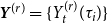 $\boldsymbol{Y}^{(r)} = \{Y_t^{(r)}(\tau _i)\}$
as the matrix of all observations of the reference country, and
$\boldsymbol{Y}^{(r)} = \{Y_t^{(r)}(\tau _i)\}$
as the matrix of all observations of the reference country, and $\boldsymbol{Y}_t^{(r)\top }$
and
$\boldsymbol{Y}_t^{(r)\top }$
and $\boldsymbol{Y}^{(r)}(\tau _i)$
are the
$\boldsymbol{Y}^{(r)}(\tau _i)$
are the $t$
-th row and
$t$
-th row and $i$
-th column of
$i$
-th column of $\boldsymbol{Y}^{(r)}$
.
$\boldsymbol{Y}^{(r)}$
.
This paper is structured to provide a comprehensive exploration of the DNS functional regression (DNS-FR) model and its applications. In Section 3, we first define the DNS model, and then extend it by adding a functional regression component to incorporate the relative spread of a reference country. Section 4 focuses on the functional transformation that transfers the functional regression to a finite-dimensional estimation problem through kPCA. Subsequently, in Sections 5 and 6, we delve into the estimation and forecasting methods, respectively. Section 7 offers an overview of the data utilized in this study. Empirical results, including the comparison of the DNS model and the DNS-FR model in terms of in-sample estimation and out-of-sample forecasting, stress testing, and a case study of a bond ladder portfolio, are presented in Section 8. Finally, Section 9 concludes.
2. Background on multicurve modeling
Previous approaches to multicurve modeling differ markedly from the framework proposed in this paper. In Diebold et al. (Reference Diebold, Li and Yue2008), multiple government bond yields were linked through an unobserved synthetic “global” yield curve – an artificial construct never used in the estimation stage. Their model employed only two factors (level and slope), with the latent global factors driving the dynamics of each country’s two-factor Nelson–Siegel process. In essence, this structure introduces common stochastic dependence across countries, but the synthetic global curve itself is redundant, as it serves no direct empirical role. Specifically, the yield of country $k$
at maturity
$k$
at maturity $\tau _i$
is given by
$\tau _i$
is given by
 \begin{align} Y_t^{(k)}(\tau _i) = L_t^{(k)} + S_t^{(k)} \left ( \frac {1 - e^{-\lambda _k \tau _i}}{\lambda _k \tau _i} \right ) + {v}_t^{(k)}(\tau _i), \end{align}
where $L_t^{(k)}$
and
$L_t^{(k)}$
and $S_t^{(k)}$
denote the level and slope factors, and
$S_t^{(k)}$
denote the level and slope factors, and ${v}_t^{(k)}(\tau _i)$
is the measurement error. The global latent factors evolve as
${v}_t^{(k)}(\tau _i)$
is the measurement error. The global latent factors evolve as
 \begin{align} \begin{bmatrix} L_t \\[5pt] S_t \end{bmatrix} = \begin{bmatrix} \Phi _{11} &\,\, \Phi _{12} \\[5pt] \Phi _{21} &\,\, \Phi _{22} \end{bmatrix} \begin{bmatrix} L_{t-1} \\[5pt] S_{t-1} \end{bmatrix} + \begin{bmatrix} \epsilon _{L,t} \\[5pt] \epsilon _{S,t} \end{bmatrix}. \end{align}
Each country’s local factors are linearly related to the global factors:
 \begin{align} L_t^{(k)} &= \alpha _L^{(k)} + \unicode{x03B2} _L^{(k)} L_t + \epsilon _{L,t}^{(k)}, \\[-12pt] \nonumber \end{align}
 \begin{align} S_t^{(k)} &= \alpha _S^{(k)} + \unicode{x03B2} _S^{(k)} S_t + \epsilon _{S,t}^{(k)}, \\[9pt] \nonumber \end{align}
where the idiosyncratic components follow AR(1) dynamics:
 \begin{align} \begin{bmatrix} \epsilon _{L,t}^{(k)} \\[8pt] \epsilon _{S,t}^{(k)} \end{bmatrix} = \begin{bmatrix} \Psi _{11}^{(k)} &\,\, \Psi _{12}^{(k)} \\[8pt] \Psi _{21}^{(k)} &\,\, \Psi _{22}^{(k)} \end{bmatrix} \begin{bmatrix} \epsilon _{L,t-1}^{(k)} \\[8pt] \epsilon _{S,t-1}^{(k)} \end{bmatrix} + \begin{bmatrix} \unicode{x03B7} _{L,t}^{(k)} \\[8pt] \unicode{x03B7} _{S,t}^{(k)} \end{bmatrix}. \end{align}
Combining these components yields
 \begin{align} Y_t^{(k)}(\tau _i) &= \alpha _L^{(k)} + \alpha _S^{(k)} \left ( \frac {1 - e^{-\lambda _k \tau _i}}{\lambda _k \tau _i} \right ) + \epsilon _{L,t}^{(k)} + \epsilon _{S,t}^{(k)} \left ( \frac {1 - e^{-\lambda _k \tau _i}}{\lambda _k \tau _i} \right ) \nonumber \\[5pt]&\quad + \unicode{x03B2} _L^{(k)} L_t + \unicode{x03B2} _S^{(k)} \left ( \frac {1 - e^{-\lambda _k \tau _i}}{\lambda _k \tau _i} \right ) S_t + v_t^{(k)}(\tau _i), \end{align}
where $Y_t^{(k)}(\tau _i)$
depends on global factors
$Y_t^{(k)}(\tau _i)$
depends on global factors $(L_t, S_t)$
and country-specific idiosyncratic terms
$(L_t, S_t)$
and country-specific idiosyncratic terms $\epsilon _{L,t}^{(k)}$
,
$\epsilon _{L,t}^{(k)}$
, $\epsilon _{S,t}^{(k)}$
.
$\epsilon _{S,t}^{(k)}$
.
Although Diebold et al. (Reference Diebold, Li and Yue2008) discuss a “global yield curve,” it is never estimated or observed, serving only as a theoretical coupling device. Without data for calibration, parameters such as $\lambda$
or the error covariance of this synthetic curve remain speculative:
$\lambda$
or the error covariance of this synthetic curve remain speculative:
 \begin{align} Y_t^{global}(\tau _i) = L_t + S_t \left ( \frac {1 - e^{\lambda \tau _i}}{\lambda \tau _i} \right ) + V_t(\tau _i), \end{align}
where $V_t(\tau _i)$
denotes noise.
$V_t(\tau _i)$
denotes noise.
In contrast, our proposed framework dispenses with synthetic constructs. We use an observed reference curve – the US Treasury yield curve – to extract functional factors that capture both tenor and temporal dependencies. This enables direct estimation and forecasting.
3. Proposed dynamic Nelson–Siegel functional regression model
We model the complete bootstrapped bond yields $Y_t(\tau _i)$
at time
$Y_t(\tau _i)$
at time $t$
with time to maturity
$t$
with time to maturity $\tau _i$
(in months) for a set
$\tau _i$
(in months) for a set $\{ \tau _1, \dots , \tau _N \}$
as follows:
$\{ \tau _1, \dots , \tau _N \}$
as follows:
 \begin{align} Y_t(\tau _i) | Y_t^{(r)}(\tau _{1\,:\,N}) & = \underbrace {F_{1,t} + F_{2,t} \left ( \frac {1 - e^{-\lambda \tau _i}}{\lambda \tau _i} \right ) + F_{3,t} \left ( \frac {1 - e^{-\lambda \tau _i}}{\lambda \tau _i} - e^{-\lambda \tau _i} \right )}_{\text{Nelson-Siegel model}} \nonumber \\[5pt]& \quad + \underbrace {\int _0^{\tau _N} \gamma _i(s) Y_{t}^{(r)}(s) ds }_{\text{Functional regression model}} +\, \epsilon _t(\tau _i) \\[-12pt] \nonumber \end{align}
 \begin{align} F_{j,t} & = \psi _{j,0} + \psi _{j,1} F_{j, t-1} + \unicode{x03B7} _{j, t}, \;\; j \in \{ 1,2,3 \}. \\[9pt] \nonumber \end{align}
Here, $\tau _N$
is the maximum maturity of the reference country’s bonds.
$\tau _N$
is the maximum maturity of the reference country’s bonds. $Y_t^{(r)}(\tau _{1\,:\,N})$
is the yield curve of reference country with maturities from
$Y_t^{(r)}(\tau _{1\,:\,N})$
is the yield curve of reference country with maturities from $\tau _1$
to
$\tau _1$
to $\tau _N$
. The parameter
$\tau _N$
. The parameter $\lambda$
governs the decay rate.
$\lambda$
governs the decay rate. $\gamma _i(s)$
represents the functional coefficient.
$\gamma _i(s)$
represents the functional coefficient. $\psi _{j,0} \in \mathbb{R}$
and
$\psi _{j,0} \in \mathbb{R}$
and $\psi _{j,1} \in (-1, 1)$
are parameters to be estimated.
$\psi _{j,1} \in (-1, 1)$
are parameters to be estimated. $\epsilon _t(\tau _i)$
and
$\epsilon _t(\tau _i)$
and $\unicode{x03B7} _{j, t}$
are independent and identically distributed normal noises. We will discuss the structures of the covariance matrices considered for both
$\unicode{x03B7} _{j, t}$
are independent and identically distributed normal noises. We will discuss the structures of the covariance matrices considered for both $\epsilon _t(\tau _i)$
and
$\epsilon _t(\tau _i)$
and $\unicode{x03B7} _{j, t}$
later in Section 4.
$\unicode{x03B7} _{j, t}$
later in Section 4.
As demonstrated, this model consists of two parts: a Nelson–Siegel model and a functional regression component. In Section 3.1, we first introduce the Nelson–Siegel model, and then in Section 3.2, we extend it by incorporating a functional regression component that captures the relative spread of a reference country’s bonds.
3.1 Dynamic Nelson–Siegel model
We begin by introducing the latent three-factor model for the yield curve, initially proposed in Nelson and Siegel (Reference Nelson and Siegel1987) and extended in Diebold and Li (Reference Diebold and Li2006) to allow time-varying factors. The efficiency of this model has been demonstrated in numerous previous works, such as Diebold et al. (Reference Diebold, Li and Yue2008), Yu and Zivot (Reference Yu and Zivot2011), and Karimalis et al. (Reference Karimalis, Kosmidis and Peters2017). The Diebold and Li (Diebold & Li, Reference Diebold and Li2006) formulation for the yield curve is given as:
 \begin{align} Y_t(\tau _i) = F_{1,t} + F_{2,t} \left ( \frac {1 - e^{-\lambda \tau _i}}{\lambda \tau _i} \right ) + F_{3,t} \left ( \frac {1 - e^{-\lambda \tau _i}}{\lambda \tau _i} - e^{-\lambda \tau _i} \right ) + \tilde {\epsilon }_t(\tau _i), \end{align}
and
 \begin{align} F_{j,t} = \psi _{j,0} + \psi _{j,1} F_{j, t-1} + \tilde {\unicode{x03B7} }_{j, t}, \;\; j \in \{ 1,2,3 \} \end{align}
for $i \in \{1, 2, \dots , N\}$
and
$i \in \{1, 2, \dots , N\}$
and $t \in \{1, 2, \dots , T\}$
. Here,
$t \in \{1, 2, \dots , T\}$
. Here, $F_{1,t}, F_{2,t}, F_{3,t}$
are three latent factors typically interpreted as level, slope, and curvature. The parameter
$F_{1,t}, F_{2,t}, F_{3,t}$
are three latent factors typically interpreted as level, slope, and curvature. The parameter $\lambda$
determines the rate of exponential decay.
$\lambda$
determines the rate of exponential decay. $\tilde {\epsilon }_t(\tau _i)$
and
$\tilde {\epsilon }_t(\tau _i)$
and $\tilde {\unicode{x03B7} }_{j, t}$
are independent and identically distributed normal noises for the measurement and state equations, respectively. Additionally, we assume that all three factors
$\tilde {\unicode{x03B7} }_{j, t}$
are independent and identically distributed normal noises for the measurement and state equations, respectively. Additionally, we assume that all three factors $F_{j,t}$
are uncorrelated. Given the dynamic nature of the hidden factors and for consistency with other works, we refer to this model as the DNS model.
$F_{j,t}$
are uncorrelated. Given the dynamic nature of the hidden factors and for consistency with other works, we refer to this model as the DNS model.
The loading on the first factor $F_{1,t}$
is always 1 and is usually called the level. It affects all yields equally, and thus it is viewed as a long-term factor. The loading on the second factor
$F_{1,t}$
is always 1 and is usually called the level. It affects all yields equally, and thus it is viewed as a long-term factor. The loading on the second factor $F_{2,t}$
is
$F_{2,t}$
is $(1 - e^{-\lambda \tau _i})/(\lambda \tau _i)$
, which starts from 1 and then decays monotonically to 0 as maturity goes to infinity, hence its called the slope or short-term factor. The loading on the third factor
$(1 - e^{-\lambda \tau _i})/(\lambda \tau _i)$
, which starts from 1 and then decays monotonically to 0 as maturity goes to infinity, hence its called the slope or short-term factor. The loading on the third factor $F_{3,t}$
is
$F_{3,t}$
is $(1 - e^{-\lambda \tau _i})/(\lambda \tau _i) - e^{-\lambda \tau _i}$
. It starts from 0, first increases, and then decays to 0 again. Therefore, it contributes mostly to medium maturities and is called the curvature or medium-term factor. Figure 1 shows the factor loadings with a fixed
$(1 - e^{-\lambda \tau _i})/(\lambda \tau _i) - e^{-\lambda \tau _i}$
. It starts from 0, first increases, and then decays to 0 again. Therefore, it contributes mostly to medium maturities and is called the curvature or medium-term factor. Figure 1 shows the factor loadings with a fixed $\lambda = 0.0609$
as in Diebold and Li (Reference Diebold and Li2006).
$\lambda = 0.0609$
as in Diebold and Li (Reference Diebold and Li2006).
Factor loadings of the DNS model with $\lambda = 0.0609$
.
$\lambda = 0.0609$
.

3.2 Functional regression representation with missing data
To address the limitation that the DNS model does not account for conditional relationships between different economies, we extend the DNS model by incorporating a functional regression component into the measurement equation. In recent years, functional data analysis (FDA) has gained popularity in time series modeling. In Hyndman and Shang (Reference Hyndman and Shang2009), such an approach was pioneered by introducing a weighted functional principal component regression method designed for forecasting functional time series. They successfully applied this method to Australian fertility rate data, representing time series curves as a finite sum of weighted hidden factors. Building on this methodology, Hays et al. (Reference Hays, Shen and Huang2012) introduced the functional dynamic factor model, which estimates both the hidden factor time series and the functional factor loadings simultaneously. This approach was applied to US Treasury yields, demonstrating superior performance compared to the DNS model. In a related study, Martınez-Hernández et al. (Reference Martınez-Hernández, Gonzalo and González-Farıas2022) proposed a nonparametric three-factor model, showing that the estimated factor loadings align with the level, slope, and curvature of the Nelson–Siegel model, highlighting the versatility and adaptability of FDA in capturing the complex dynamics of yield curves. The applications of the FDA in the interest rate market were explored in Bowsher and Meeks (Reference Bowsher and Meeks2008) and Jiang (Reference Jiang2014).
It is noteworthy that, in reality, data are often incomplete. In the presence of missing data, bootstrapping methods are commonly used to handle the gaps. Different bootstrapping methods were discussed in Ametrano and Bianchetti (Reference Ametrano and Bianchetti2013) and Peters and Loke (Reference Peters and Loken.d.). In this paper, missing data can occur in both the reference country-specific yields $Y_t^{(r)}(\tau _i)$
and the response country-specific yields
$Y_t^{(r)}(\tau _i)$
and the response country-specific yields $Y_t(\tau _i)$
. For the former, given the small amount of missing data in our datasets, we use linear interpolation to fill in the missing values for simplicity. For the latter, we define a binary variable
$Y_t(\tau _i)$
. For the former, given the small amount of missing data in our datasets, we use linear interpolation to fill in the missing values for simplicity. For the latter, we define a binary variable $S_{ti}$
to track the missing data:
$S_{ti}$
to track the missing data:
 \begin{equation*} S_{ti} = \begin{cases} 1 \quad \text{if} \; Y_t(\tau _i) \; \text{is recorded} \\ 0 \quad \text{otherwise.} \end{cases} \end{equation*}
The extended model is given as:
 \begin{align} \tilde {Y}_t(\tau _i) | Y_{t}^{(r)}({\cdot}) & = \left [ F_{1,t} + F_{2,t} \left ( \frac {1 - e^{-\lambda \tau _i}}{\lambda \tau _i} \right ) + F_{3,t} \left ( \frac {1 - e^{-\lambda \tau _i}}{\lambda \tau _i} - e^{-\lambda \tau _i} \right ) \right. \nonumber \\ & \quad \left. + \int _0^{\tau _N} \gamma _i(s) Y_{t}^{(r)}(s) ds + \epsilon _t(\tau _i) \right ] \cdot S_{ti}, \end{align}
and the state equation remains unchanged:
 \begin{align} F_{j,t} = \psi _{j,0} + \psi _{j,1} F_{j, t-1} + \unicode{x03B7} _{j, t}, \;\; j \in \{ 1,2,3 \}. \end{align}
If data are complete, this model reduces to Equations (8) and (9). Here, $Y_{t}^{(r)}(s)$
represents the yield curve of a reference country at time
$Y_{t}^{(r)}(s)$
represents the yield curve of a reference country at time $t$
, and
$t$
, and $\gamma _i(s)$
are the functional coefficients. In this study, we assume that the yield curve of the response country at time
$\gamma _i(s)$
are the functional coefficients. In this study, we assume that the yield curve of the response country at time $t$
depends only on the yield curve of the reference country at the current time
$t$
depends only on the yield curve of the reference country at the current time $t$
and not on previous times. Additionally, we assume that the functional coefficient
$t$
and not on previous times. Additionally, we assume that the functional coefficient $\gamma _i(s)$
is time-invariant and varies across different maturities of bonds from the response country. We refer to this model as the DNS-FR model.
$\gamma _i(s)$
is time-invariant and varies across different maturities of bonds from the response country. We refer to this model as the DNS-FR model.
However, estimating the functional coefficient $\gamma _i(s)$
is challenging. Therefore, in the next section, we will transform the functional regression component into a weighted sum of a finite number of factors.
$\gamma _i(s)$
is challenging. Therefore, in the next section, we will transform the functional regression component into a weighted sum of a finite number of factors.
4. Functional representation and transformation
In order to transform the integral representation of the functional regression into a vector operation suitable for linear estimation, this section introduces the kPCA method. The kPCA procedure is employed to extract a finite set of factors from the yields of the reference country. Compared with traditional PCA, kPCA offers a key advantage in capturing nonlinear structures within the data while effectively reducing dimensionality. A similar methodology has been applied in the modeling of green bonds in Campi et al. (Reference Campi, Peters and Richards2024). The detailed derivation of the kPCA procedure is provided in Appendix A.
Consider the bootstrapped input matrix of bond yields for the reference country:
 \begin{equation*} \boldsymbol{Y}_{N \times T}^{(r)} = \left [ \begin{array}{c@{\quad}c@{\quad}l@{\quad}c} Y_1^{(r)}(\tau _1) & Y_2^{(r)}(\tau _1) & \cdots & Y_T^{(r)}(\tau _1) \\[7pt] Y_1^{(r)}(\tau _2) & Y_2^{(r)}(\tau _2) & \cdots & Y_T^{(r)}(\tau _2) \\[7pt] \vdots & \vdots & \ddots & \vdots \\[7pt] Y_1^{(r)}(\tau _N) & Y_2^{(r)}(\tau _N) & \cdots & Y_T^{(r)}(\tau _N) \end{array} \right ]. \end{equation*}
We denote $\boldsymbol{Y}^{(r)}(\tau _i) = \left [ Y_1^{(r)}(\tau _i), Y_2^{(r)}(\tau _i), \dots , Y_T^{(r)}(\tau _i) \right ]^\top$
as the time series of the yields of the bonds with maturity
$\boldsymbol{Y}^{(r)}(\tau _i) = \left [ Y_1^{(r)}(\tau _i), Y_2^{(r)}(\tau _i), \dots , Y_T^{(r)}(\tau _i) \right ]^\top$
as the time series of the yields of the bonds with maturity $\tau _i$
. Assume
$\tau _i$
. Assume $\boldsymbol{\unicode{x03D5} }\,:\, \mathcal{Y} \to \mathcal{F}$
is a nonlinear mapping from the observed input space
$\boldsymbol{\unicode{x03D5} }\,:\, \mathcal{Y} \to \mathcal{F}$
is a nonlinear mapping from the observed input space $\mathcal{Y} \subset \mathbb{R}^T$
to the feature space
$\mathcal{Y} \subset \mathbb{R}^T$
to the feature space $\mathcal{F} \subset \mathbb{R}^T$
such that
$\mathcal{F} \subset \mathbb{R}^T$
such that $\unicode{x1D6DF}(\boldsymbol{Y}^{(r)}(\tau _i)) = \left [ \unicode{x03D5} _1(\boldsymbol{Y}^{(r)}(\tau _i)), \dots , \unicode{x03D5} _T(\boldsymbol{Y}^{(r)}(\tau _i)) \right ]^\top$
.
$\unicode{x1D6DF}(\boldsymbol{Y}^{(r)}(\tau _i)) = \left [ \unicode{x03D5} _1(\boldsymbol{Y}^{(r)}(\tau _i)), \dots , \unicode{x03D5} _T(\boldsymbol{Y}^{(r)}(\tau _i)) \right ]^\top$
.
Let $\boldsymbol{\Phi }$
be an
$\boldsymbol{\Phi }$
be an $N \times T$
matrix:
$N \times T$
matrix:
 \begin{equation*} \boldsymbol{\Phi }_{N \times T} = \left [ \begin{array}{c@{\quad}l@{\quad}c} \unicode{x03D5} _1(\boldsymbol{Y}^{(r)}(\tau _1)) & \cdots & \unicode{x03D5} _T(\boldsymbol{Y}^{(r)}(\tau _1)) \\[7pt] \vdots & \ddots & \vdots \\[7pt] \unicode{x03D5} _1(\boldsymbol{Y}^{(r)}(\tau _N)) & \cdots & \unicode{x03D5} _T(\boldsymbol{Y}^{(r)}(\tau _N)) \end{array} \right ]. \end{equation*}
The objective of kPCA is to find a linear projection that projects $\boldsymbol{\Phi }$
onto uncorrelated components denoted
$\boldsymbol{\Phi }$
onto uncorrelated components denoted $\boldsymbol{A}$
, with lower dimensionality. Each point
$\boldsymbol{A}$
, with lower dimensionality. Each point $\unicode{x1D6DF}(\boldsymbol{Y}^{(r)}(\tau _i))$
can be expressed as a linear combination of
$\unicode{x1D6DF}(\boldsymbol{Y}^{(r)}(\tau _i))$
can be expressed as a linear combination of $Q \le T$
vectors of dimension
$Q \le T$
vectors of dimension $T$
:
$T$
:
 \begin{equation*} \unicode{x1D6DF}(\boldsymbol{Y}^{(r)}(\tau _i)) = \sum _{q=1}^Q \alpha _{i,q} \boldsymbol{v}_q, \end{equation*}
where $\boldsymbol{v}_q$
are orthonormal basis vectors, and the coefficient vectors
$\boldsymbol{v}_q$
are orthonormal basis vectors, and the coefficient vectors ${\boldsymbol{\alpha }}_q = [ \alpha _{1,q}, \dots , \alpha _{N,q}]^\top$
satisfy
${\boldsymbol{\alpha }}_q = [ \alpha _{1,q}, \dots , \alpha _{N,q}]^\top$
satisfy
 \begin{equation*} {\boldsymbol{\alpha }}_q^\top {\boldsymbol{\alpha }}_q = \sum _{i=1}^{N} \alpha _{i,q}^2 = \lambda _q, \end{equation*}
with $\lambda _q$
being the
$\lambda _q$
being the $q$
th eigenvalue of
$q$
th eigenvalue of $\boldsymbol{\Phi ^\top \Phi }$
.
$\boldsymbol{\Phi ^\top \Phi }$
.
In practice, the explicit form of the mapping $\unicode{x1D6DF}({\cdot})$
is typically unknown, and thus
$\unicode{x1D6DF}({\cdot})$
is typically unknown, and thus $\lambda _q$
and
$\lambda _q$
and $\boldsymbol{v}_q$
cannot be computed directly. To address this, we introduce a kernel function
$\boldsymbol{v}_q$
cannot be computed directly. To address this, we introduce a kernel function $k \,:\, \mathcal{Y} \times \mathcal{Y} \to \mathcal{F}$
, which defines the inner product in the feature space
$k \,:\, \mathcal{Y} \times \mathcal{Y} \to \mathcal{F}$
, which defines the inner product in the feature space $\mathcal{F}$
:
$\mathcal{F}$
:
 \begin{align} k(\boldsymbol{Y}^{(r)}(\tau _i), \boldsymbol{Y}^{(r)}(\tau _j)) = \unicode{x1D6DF}(\boldsymbol{Y}^{(r)}(\tau _i))^\top \unicode{x1D6DF}(\boldsymbol{Y}^{(r)}(\tau _j)) = \sum _{k=1}^T \unicode{x03D5} _k(\boldsymbol{Y}^{(r)}(\tau _i)) \unicode{x03D5} _k(\boldsymbol{Y}^{(r)}(\tau _j)) \end{align}
for $i, j \in \{ 1, \dots , N \}$
. Using standard matrix algebra, the eigenvectors can then be expressed as
$i, j \in \{ 1, \dots , N \}$
. Using standard matrix algebra, the eigenvectors can then be expressed as
 \begin{equation*} \boldsymbol{v}_q^\top = \sum _{i=1}^N w_{i,q} \unicode{x1D6DF}(\boldsymbol{Y}^{(r)}(\tau _i)), \end{equation*}
and the principal component is given by
 \begin{align} \alpha _{m,q} = \sum _{i=1}^N w_{i,q} k(\boldsymbol{Y}^{(r)}(\tau _m), \boldsymbol{Y}^{(r)}(\tau _i)), \end{align}
where $w_{i,q}$
denotes the weights. For a new sample
$w_{i,q}$
denotes the weights. For a new sample $\boldsymbol{Y}(\tau ^*)$
, where
$\boldsymbol{Y}(\tau ^*)$
, where $\tau ^* \notin \{ \tau _1, \dots , \tau _N \}$
and
$\tau ^* \notin \{ \tau _1, \dots , \tau _N \}$
and $\tau ^* \in [0, \tau _{max}]$
, the projection onto the
$\tau ^* \in [0, \tau _{max}]$
, the projection onto the $q$
th component is
$q$
th component is
 \begin{align} \alpha _{*, q} = \sum _{i=1}^N w_{i,q} k(\boldsymbol{Y}(\tau ^*), \boldsymbol{Y}(\tau _i)). \end{align}
In this paper, we choose the radial basis function (RBF) kernel, which is of the form
 \begin{align} k(\boldsymbol{x},\boldsymbol{Y}) = \exp {\left (- \iota ||\boldsymbol{x}-\boldsymbol{Y}||^2 \right )}, \end{align}
where $\iota \gt 0$
is the hyperparameter. We will discuss the estimation of
$\iota \gt 0$
is the hyperparameter. We will discuss the estimation of $\iota$
in Section 5.1. The validation of the RBF kernel is proved in Shawe-Taylor and Cristianini (Reference Shawe-Taylor and Cristianini2004). Here, we choose the RBF kernel because it is both universal (Wang et al., Reference Wang, Chen and Chen2004; Ismayilova & Ismayilov, Reference Ismayilova and Ismayilov2024) and characteristic (Sriperumbudur et al., Reference Sriperumbudur, Fukumizu and Lanckriet2011; Szabó & Sriperumbudur, Reference Szabó and Sriperumbudur2018). A universal kernel means that it can approximate any continuous function on a compact domain, while a characteristic kernel ensures that it uniquely distinguishes probability distributions. Other popular kernel function options include the polynomial kernel, Square Bessel kernel, graph kernel, and ANOVA kernel, though these other kernel choices, whilst widely used, are typically not provably characteristic and universal.
$\iota$
in Section 5.1. The validation of the RBF kernel is proved in Shawe-Taylor and Cristianini (Reference Shawe-Taylor and Cristianini2004). Here, we choose the RBF kernel because it is both universal (Wang et al., Reference Wang, Chen and Chen2004; Ismayilova & Ismayilov, Reference Ismayilova and Ismayilov2024) and characteristic (Sriperumbudur et al., Reference Sriperumbudur, Fukumizu and Lanckriet2011; Szabó & Sriperumbudur, Reference Szabó and Sriperumbudur2018). A universal kernel means that it can approximate any continuous function on a compact domain, while a characteristic kernel ensures that it uniquely distinguishes probability distributions. Other popular kernel function options include the polynomial kernel, Square Bessel kernel, graph kernel, and ANOVA kernel, though these other kernel choices, whilst widely used, are typically not provably characteristic and universal.
The standard approach to learning hyperparameters of the kernel in such a regression setting is via either maximum likelihood procedures or cross-validation methods. In this work, we adopted a nonlinear maximum likelihood procedure, with a simple and reliable 2-dimensional grid search procedure. Details are available in the GitHub repository accompanying this manuscript.Footnote 1
Subsequently, the functional regression term in Equation (8) is expressed as a weighted sum of a finite number of factors by applying the Karhunen-Loeve theorem:
Theorem 1 (Karhunen-Loeve theorem). Suppose $X_t$
is a zero-mean stochastic process for
$X_t$
is a zero-mean stochastic process for $t \in [a, b]$
.
$t \in [a, b]$
. $K(s,t)$
is the continuous covariance function. Then
$K(s,t)$
is the continuous covariance function. Then $X_t$
can be expressed as
$X_t$
can be expressed as
 \begin{equation*} X_t = \sum _{j=1}^\infty Z_j e_j(t), \end{equation*}
where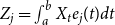 $Z_j = \int _a^b X_t e_j(t) dt$
and
$Z_j = \int _a^b X_t e_j(t) dt$
and $e_j(t)$
are orthonormal basis functions defined in (18).
$e_j(t)$
are orthonormal basis functions defined in (18).
The orthonormal functions are defined as follows:
Definition 1.
Two real-valued functions $f(x)$
and
$f(x)$
and $g(x)$
are orthonormal over the interval
$g(x)$
are orthonormal over the interval $[a,b]$
if
$[a,b]$
if
-
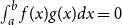
1. $\int _a^b f(x) g(x) dx = 0$
-
2.
$||f(x)||_2 = ||g(x)||_2 = \left [ \int _a^b |f(x)|^2 dx \right ]^{1/2} = \left [ \int _a^b |g(x)|^2 dx \right ]^{1/2} = 1$

In this paper, we choose $e_q(\tau _i) = \alpha _{i,q} \boldsymbol{v}_q$
Footnote 2 as the orthogonal basis functions, so that
$e_q(\tau _i) = \alpha _{i,q} \boldsymbol{v}_q$
Footnote 2 as the orthogonal basis functions, so that $\unicode{x1D6DF} (\boldsymbol{Y}^{(r)}(\tau _i))$ $= \sum _{q=1}^Q e_q(\tau _i)$
. Therefore, we have
$= \sum _{q=1}^Q e_q(\tau _i)$
. Therefore, we have
 \begin{align} e_q(\tau _i) = \alpha _{i,q} \boldsymbol{v}_q = \sum _{j=1}^N w_{j,q} k(\boldsymbol{Y}^{(r)}(\tau _i), \boldsymbol{Y}^{(r)}(\tau _j)) \boldsymbol{v}_q. \end{align}
Using the Karhunen-Loeve theorem, we express $Y_t^{(r)}(s)$
and
$Y_t^{(r)}(s)$
and $\gamma _i(s)$
as follows:
$\gamma _i(s)$
as follows:
 \begin{align} Y_t^{(r)}(s) = \sum _{j=1}^\infty U_{tj} e_j(s) \end{align}
and
 \begin{align} \gamma _i(s) = \sum _{k=1}^\infty \gamma _{i,k} e_k(s), \end{align}
where $U_{tj} = \int _0^{\tau _N} Y_t^{(r)}(s) e_j(s) ds$
and
$U_{tj} = \int _0^{\tau _N} Y_t^{(r)}(s) e_j(s) ds$
and $\gamma _{i,k} = \int _0^{\tau _N} \gamma _i(s) e_k(s) ds$
. We then have:
$\gamma _{i,k} = \int _0^{\tau _N} \gamma _i(s) e_k(s) ds$
. We then have:
 \begin{align} \int _0^{\tau _N} \gamma _i(s) Y_t^{(r)}(s) ds =& \int _0^{\tau _N} \left ( \sum _{k=1}^\infty \gamma _{i,k} e_k(s) \right ) \left ( \sum _{j=1}^\infty U_{tj} e_j(s) \right ) ds \nonumber \\ =& \sum _{j=k, j=1}^\infty \gamma _{i,j} U_{tj} \int _0^{\tau _N} \left ( e_j(s) \right )^2 ds + \sum _{j \ne k} \gamma _{i,k} U_{tj} \int _0^{\tau _N} e_k(s) e_j(s) ds \nonumber \\ =& \sum _{j=1}^\infty \gamma _{i,j} U_{tj} \approx \sum _{j=1}^Q \gamma _{i,j} U_{tj}. \end{align}
Thus, the DNS-FR model given in Equations (8) and (9) can be rewritten as:
 \begin{align} Y_t(\tau _i) & = F_{1,t} + F_{2,t} \left ( \frac {1 - e^{-\lambda \tau _i}}{\lambda \tau _i} \right ) + F_{3,t} \left ( \frac {1 - e^{-\lambda \tau _i}}{\lambda \tau _i} - e^{-\lambda \tau _i} \right ) + \sum _{j=1}^Q \gamma _{i,j} U_{tj} + \epsilon _t(\tau _i), \\[-28pt] \nonumber \end{align}
 \begin{align} F_{j,t} & = \psi _{j,0} + \psi _{j,1} F_{j, t-1} + \unicode{x03B7} _{j, t}, \;\; j \in \{ 1,2,3 \}. \\[0pt] \nonumber \end{align}
In matrix notation, this becomes:
 \begin{align} \boldsymbol{Y}_t &= \boldsymbol{\Lambda } \boldsymbol{F}_t + \boldsymbol{\Gamma } \boldsymbol{U}_t + \boldsymbol{\epsilon }_t, \;\; \boldsymbol{\epsilon }_t \sim N(0, \boldsymbol{\Sigma }_{\epsilon }), \\[-12pt] \nonumber \end{align}
 \begin{align} \boldsymbol{F}_t &= \boldsymbol{\Psi }_0 + \boldsymbol{\Psi }_1 \boldsymbol{F}_{t-1} + \boldsymbol{\unicode{x03B7} }_t, \;\; \boldsymbol{\unicode{x03B7} }_t \sim N(0, \boldsymbol{\Sigma }_{\unicode{x03B7} }). \\[9pt] \nonumber \end{align}
Given the assumptions that the $F_{j,t}$
are uncorrelated, we have:
$F_{j,t}$
are uncorrelated, we have:
 \begin{equation*} \boldsymbol{\Sigma }_{\unicode{x03B7} } = \left [ \begin{matrix} \sigma _{\unicode{x03B7} _1}^2 &\,\,\, 0 &\,\,\, 0 \\[5pt] 0 &\,\,\, \sigma _{\unicode{x03B7} _2}^2 &\,\,\, 0 \\[5pt] 0 &\,\,\, 0 &\,\,\, \sigma _{\unicode{x03B7} _3}^2 \end{matrix} \right ]. \end{equation*}
However, $\boldsymbol{\Sigma }_{\epsilon }$
is not, generally, a diagonal matrix. That is because in the bond market, different bonds with different maturities are usually correlated to each other. Therefore, in this paper, we will consider the following three structures for
$\boldsymbol{\Sigma }_{\epsilon }$
is not, generally, a diagonal matrix. That is because in the bond market, different bonds with different maturities are usually correlated to each other. Therefore, in this paper, we will consider the following three structures for $\boldsymbol{\Sigma }_{\epsilon }$
, for both the DNS model and the DNS-FR model:
$\boldsymbol{\Sigma }_{\epsilon }$
, for both the DNS model and the DNS-FR model:
-
1.
$\boldsymbol{\Sigma }_{\epsilon }$
is diagonal, and bonds with different maturities have different variances:
\begin{equation*} \boldsymbol{\Sigma }_{\epsilon } = \left [ \begin{array}{c@{\quad}c@{\quad}l@{\quad}c} \sigma _{\epsilon _1}^2 & 0 & \cdots & 0 \\[5pt] 0 & \sigma _{\epsilon _2}^2 & \cdots & 0 \\[5pt] \vdots & \vdots & \ddots & \vdots \\[5pt] 0 & 0 & \cdots & \sigma _{\epsilon _N}^2 \end{array} \right ]. \end{equation*}
-
2.
$\boldsymbol{\Sigma }_{\epsilon }$
has a diagonal band. Each bond is only correlated to the two bonds (one with shorter maturity, and one with longer maturity) which are closest to it, but is not correlated to others. Furthermore, we assume that all pairs of two adjacent bonds have the same correlation coefficient:However, it should be noted that this matrix is not always positive definite for all
\begin{equation*} \boldsymbol{\Sigma }_{\epsilon } = \left [ \begin{array}{c@{\quad}c@{\quad}c@{\quad}l@{\quad}c@{\quad}c} \sigma _{\epsilon _1}^2 & \unicode{x03C1} \sigma _{\epsilon _1} \sigma _{\epsilon _2} & 0 & \cdots & 0 & 0 \\[5pt] \unicode{x03C1} \sigma _{\epsilon _1} \sigma _{\epsilon _2} & \sigma _{\epsilon _2}^2 & \unicode{x03C1} \sigma _{\epsilon _2} \sigma _{\epsilon _3} & \cdots & 0 & 0 \\[5pt] 0 & \unicode{x03C1} \sigma _{\epsilon _2} \sigma _{\epsilon _3} & \sigma _{\epsilon _3}^2 & \cdots & 0 & 0 \\[5pt] \vdots & \vdots & \vdots & \ddots & \vdots \\[5pt] 0 & 0 & 0 & \cdots & \sigma _{\epsilon _{N-1}}^2 & \unicode{x03C1} \sigma _{\epsilon _{N-1}} \sigma _{\epsilon _N} \\[5pt] 0 & 0 & 0 & \cdots & \unicode{x03C1} \sigma _{\epsilon _{N-1}} \sigma _{\epsilon _N} & \sigma _{\epsilon _N}^2 \end{array} \right ] \end{equation*}
$\unicode{x03C1} \in [-1, 1]$
. Actually, it has been shown in Johnson et al. (Reference Johnson, Neumann and Tsatsomeros1996) that only when
$\unicode{x03C1}$
ranges from
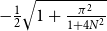
$-\frac {1}{2} \sqrt {1 + \frac {\pi ^2}{1 + 4N^2}}$
to
$\frac {1}{2} \sqrt {1 + \frac {\pi ^2}{1 + 4N^2}}$
, a positive definite matrix is guaranteed. Therefore, assuming
$\theta \in \mathbb{R}$
is the input parameter, we take a transformation(26)to make sure that
\begin{align} \unicode{x03C1} = \sqrt {1 + \frac {\pi ^2}{1 + 4N^2}} \times \frac {1}{1 + e^{-\theta }} - \frac {1}{2} \sqrt {1 + \frac {\pi ^2}{1 + 4N^2}} \end{align}
$\unicode{x03C1}$
is in the correct range.
-
3.
$\boldsymbol{\Sigma }_{\epsilon }$
is a full covariance matrix. To avoid a very high dimensionality of parameter space, we assume that this covariance is generated by two parameters in the following form:In this case, we assume that all bonds have the same variance, and the covariance of two bonds decays as the difference in maturities increases.
\begin{equation*} \boldsymbol{\Sigma }_{\epsilon } = \left [ \begin{array}{c@{\quad}c@{\quad}l@{\quad}c} \sigma ^2 & \sigma ^2 \unicode{x03C1} & \cdots & \sigma ^2 \unicode{x03C1} ^{N-1} \\[5pt] \sigma ^2 \unicode{x03C1} & \sigma ^2 & \cdots & \sigma ^2 \unicode{x03C1} ^{N-2} \\[5pt] \vdots & \vdots & \ddots & \vdots \\[5pt] \sigma ^2 \unicode{x03C1} ^{N-1} & \sigma ^2 \unicode{x03C1} ^{N-2} & \cdots & \sigma ^2 \end{array} \right ] \end{equation*}




In Section 8, we will compare the in-sample estimation accuracy of the models using these three covariance structures, respectively.
5. Estimation methodology
In this section, we present the estimation methods for the model. We first discuss the estimation of the hyperparameter $\iota$
of the RBF kernel function in Section 5.1. Then, in Section 5.2, we introduce the Kalman Filter to estimate the hidden factors in a standard linear state-space model. All parameters of the state-space model are estimated by maximizing the marginal likelihood function in Sections 5.3 and 5.4.
$\iota$
of the RBF kernel function in Section 5.1. Then, in Section 5.2, we introduce the Kalman Filter to estimate the hidden factors in a standard linear state-space model. All parameters of the state-space model are estimated by maximizing the marginal likelihood function in Sections 5.3 and 5.4.
5.1 Estimation of hyperparameters for the Kernel function
The hyperparameter $\iota$
of the RBF kernel is estimated through a grid search. We choose
$\iota$
of the RBF kernel is estimated through a grid search. We choose $\iota$
from the range 0.001 to 1 with a step size of 0.001. At each grid point, the pre-image measurement error is calculated. The point on the grid with the minimum error is selected as the optimal
$\iota$
from the range 0.001 to 1 with a step size of 0.001. At each grid point, the pre-image measurement error is calculated. The point on the grid with the minimum error is selected as the optimal $\iota$
.
$\iota$
.
To prevent data leakage, the hyperparameter $\iota$
and all other model parameters are estimated exclusively using in-sample observations. Out-of-sample forecasts are then generated sequentially, conditioning only on the historical information available at each forecasting point. Moreover, the factors
$\iota$
and all other model parameters are estimated exclusively using in-sample observations. Out-of-sample forecasts are then generated sequentially, conditioning only on the historical information available at each forecasting point. Moreover, the factors $U_{tj}$
are estimated using kPCA based solely on in-sample data during the in-sample estimation stage, while in the out-of-sample forecasting stage, these factors are reconstructed using both in-sample and out-of-sample data.
$U_{tj}$
are estimated using kPCA based solely on in-sample data during the in-sample estimation stage, while in the out-of-sample forecasting stage, these factors are reconstructed using both in-sample and out-of-sample data.
5.2 Kalman Filter
The Kalman Filter is used to estimate all parameters of the DNS-FR model. We start by reparameterizing Equations (24) and (25) into a standard state-space model:
 \begin{align} &\boldsymbol{Y}_t - \boldsymbol{\Lambda \mu } - \boldsymbol{\Gamma } \boldsymbol{U}_t = \boldsymbol{\Lambda } (\boldsymbol{F}_t - \boldsymbol{\mu }) + \boldsymbol{B} \boldsymbol{v}_t, \\[-28pt] \nonumber \end{align}
 \begin{align} &\boldsymbol{F}_t - \boldsymbol{\mu } = \boldsymbol{\Psi }_1 (\boldsymbol{F}_{t-1} - \boldsymbol{\mu }) + \boldsymbol{D} \boldsymbol{w}_t, \\[0pt] \nonumber \end{align}
where $\boldsymbol{\mu }$
is the mean vector of the hidden state vector such that
$\boldsymbol{\mu }$
is the mean vector of the hidden state vector such that $\boldsymbol{\mu } - \boldsymbol{\Psi }_1 \boldsymbol{\mu } = \boldsymbol{\Psi }_0$
, and
$\boldsymbol{\mu } - \boldsymbol{\Psi }_1 \boldsymbol{\mu } = \boldsymbol{\Psi }_0$
, and $\boldsymbol{B}$
and
$\boldsymbol{B}$
and $\boldsymbol{D}$
are Cholesky decomposition of
$\boldsymbol{D}$
are Cholesky decomposition of $\boldsymbol{\Sigma }_{\epsilon }$
and
$\boldsymbol{\Sigma }_{\epsilon }$
and $\boldsymbol{\Sigma }_{\unicode{x03B7} }$
, respectively.
$\boldsymbol{\Sigma }_{\unicode{x03B7} }$
, respectively. $\boldsymbol{v}_t$
and
$\boldsymbol{v}_t$
and $\boldsymbol{w}_t$
are uncorrelated unit-variance white noise processes. We define
$\boldsymbol{w}_t$
are uncorrelated unit-variance white noise processes. We define $\boldsymbol{Z}_t \,:\!=\, \boldsymbol{Y}_t - \boldsymbol{\Lambda \mu } - \boldsymbol{\Gamma } \boldsymbol{U}_t$
and
$\boldsymbol{Z}_t \,:\!=\, \boldsymbol{Y}_t - \boldsymbol{\Lambda \mu } - \boldsymbol{\Gamma } \boldsymbol{U}_t$
and $\boldsymbol{X}_t \,:\!=\, \boldsymbol{F}_t - \boldsymbol{\mu }$
representing the measurement and state vectors. Therefore, Equations (27) and (28) can be rewritten as:
$\boldsymbol{X}_t \,:\!=\, \boldsymbol{F}_t - \boldsymbol{\mu }$
representing the measurement and state vectors. Therefore, Equations (27) and (28) can be rewritten as:
 \begin{align} &\boldsymbol{Z}_t = \boldsymbol{\Lambda } \boldsymbol{X}_t + \boldsymbol{B} \boldsymbol{v}_t, \\[-28pt] \nonumber \end{align}
 \begin{align} &\boldsymbol{X}_t = \boldsymbol{\Psi }_1 \boldsymbol{X}_{t-1} + \boldsymbol{D} \boldsymbol{w}_t. \\[0pt] \nonumber \end{align}
For the DNS model, we have similar notations but $\boldsymbol{\Gamma } \boldsymbol{U}_t = 0$
.
$\boldsymbol{\Gamma } \boldsymbol{U}_t = 0$
.
Moreover, we use the following notations to represent the expectation and covariance matrix of the state vector $\boldsymbol{X}_t$
:
$\boldsymbol{X}_t$
:
 \begin{align*} \boldsymbol{a}_{t|t-1} &\,:\!=\, \mathbb{E}(\boldsymbol{X}_t | \boldsymbol{Z}_{1\,:\,t-1}), \qquad \boldsymbol{P}_{t|t-1} \,:\!=\, Cov(\boldsymbol{X}_t | \boldsymbol{Z}_{1\,:\,t-1}), \\\boldsymbol{a}_t &\,:\!=\, \mathbb{E}(\boldsymbol{X}_t | \boldsymbol{Z}_{1\,:\,t}), \qquad \kern24pt \boldsymbol{P}_t \,:\!=\, Cov(\boldsymbol{X}_t | \boldsymbol{Z}_{1\,:\,t}) \end{align*} $\boldsymbol{Z}_{1\,:\,t}$
represents all vectors
$\boldsymbol{Z}_{1\,:\,t}$
represents all vectors $\boldsymbol{Z}_{1}, \boldsymbol{Z}_{2}, \dots , \boldsymbol{Z}_{t}$
. We assume that
$\boldsymbol{Z}_{1}, \boldsymbol{Z}_{2}, \dots , \boldsymbol{Z}_{t}$
. We assume that $\boldsymbol{X}_t$
is a Markov process, so that the distribution at time
$\boldsymbol{X}_t$
is a Markov process, so that the distribution at time $t$
depends only on the state in the previous time
$t$
depends only on the state in the previous time $t-1$
.
$t-1$
.
Now, we present the algorithm of the Kalman Filter. The system starts from an initial state $\boldsymbol{X}_0 \sim N(\boldsymbol{a}_0, \boldsymbol{P}_0)$
, and all point estimates
$\boldsymbol{X}_0 \sim N(\boldsymbol{a}_0, \boldsymbol{P}_0)$
, and all point estimates $\boldsymbol{a}_t$
and covariance
$\boldsymbol{a}_t$
and covariance $\boldsymbol{P}_t$
are calculated recursively in a two-stage process involving a prediction stage and a update stage.
$\boldsymbol{P}_t$
are calculated recursively in a two-stage process involving a prediction stage and a update stage.
First, given observations $\boldsymbol{Z}_{1\,:\,t-1}$
and state
$\boldsymbol{Z}_{1\,:\,t-1}$
and state $\boldsymbol{X}_{t-1}$
, the prediction of the distribution of
$\boldsymbol{X}_{t-1}$
, the prediction of the distribution of $\boldsymbol{X}_t$
is calculated by
$\boldsymbol{X}_t$
is calculated by
 \begin{align} f(\boldsymbol{X}_t | \boldsymbol{Z}_{1\,:\,t-1}) = \int f(\boldsymbol{X}_{t} | \boldsymbol{X}_{t-1}, \boldsymbol{Z}_{1\,:\,t-1}) f(\boldsymbol{X}_{t-1} | \boldsymbol{Z}_{1\,:\,t-1}) d \boldsymbol{X}_{t-1}, \end{align}
where $f({\cdot})$
represents the density function. As
$f({\cdot})$
represents the density function. As $\boldsymbol{X}_{t} | \boldsymbol{X}_{t-1}, \boldsymbol{Z}_{1\,:\,t-1} \sim N(\boldsymbol{\Psi }_1 \boldsymbol{X}_{t-1}, \boldsymbol{\Sigma }_{\unicode{x03B7} })$
and
$\boldsymbol{X}_{t} | \boldsymbol{X}_{t-1}, \boldsymbol{Z}_{1\,:\,t-1} \sim N(\boldsymbol{\Psi }_1 \boldsymbol{X}_{t-1}, \boldsymbol{\Sigma }_{\unicode{x03B7} })$
and $\boldsymbol{X}_{t-1} | \boldsymbol{Z}_{1\,:\,t-1} \sim N(\boldsymbol{a}_{t-1}, \boldsymbol{P}_{t-1})$
, we have
$\boldsymbol{X}_{t-1} | \boldsymbol{Z}_{1\,:\,t-1} \sim N(\boldsymbol{a}_{t-1}, \boldsymbol{P}_{t-1})$
, we have $\boldsymbol{X}_t | \boldsymbol{Z}_{1\,:\,t-1} \sim N(\boldsymbol{\Psi }_1 \boldsymbol{a}_{t-1}, \boldsymbol{\Psi }_1 \boldsymbol{P}_{t-1} \boldsymbol{\Psi }_1^\top + \boldsymbol{\Sigma }_{\unicode{x03B7} })$
. The point estimates and the covariance matrix are
$\boldsymbol{X}_t | \boldsymbol{Z}_{1\,:\,t-1} \sim N(\boldsymbol{\Psi }_1 \boldsymbol{a}_{t-1}, \boldsymbol{\Psi }_1 \boldsymbol{P}_{t-1} \boldsymbol{\Psi }_1^\top + \boldsymbol{\Sigma }_{\unicode{x03B7} })$
. The point estimates and the covariance matrix are
 \begin{align} \boldsymbol{a}_{t|t-1} = \boldsymbol{\Psi }_1 \boldsymbol{a}_{t-1} \end{align}
and
 \begin{align} \boldsymbol{P}_{t|t-1} = \boldsymbol{\Psi }_1 \boldsymbol{P}_{t-1} \boldsymbol{\Psi }_1^\top + \boldsymbol{\Sigma }_{\unicode{x03B7} }. \end{align}
Next, when a new observation $\boldsymbol{Z}_t$
is available, we update the distribution as
$\boldsymbol{Z}_t$
is available, we update the distribution as
 \begin{align} f(\boldsymbol{X}_t | \boldsymbol{Z}_{1\,:\,t}) \propto f(\boldsymbol{Z}_t | \boldsymbol{X}_{t}, \boldsymbol{Z}_{1\,:\,t-1}) f(\boldsymbol{X}_t | \boldsymbol{Z}_{1\,:\,t-1}), \end{align}
which is a direct result of Bayes’ Theorem. From the measurement equation, we have $\boldsymbol{Z}_t | \boldsymbol{X}_{t}, \boldsymbol{Z}_{1\,:\,t-1} \sim N(\boldsymbol{\Lambda } \boldsymbol{X}_t, \boldsymbol{\Sigma }_{\epsilon })$
. Then, using some basic properties of normal distribution, we have
$\boldsymbol{Z}_t | \boldsymbol{X}_{t}, \boldsymbol{Z}_{1\,:\,t-1} \sim N(\boldsymbol{\Lambda } \boldsymbol{X}_t, \boldsymbol{\Sigma }_{\epsilon })$
. Then, using some basic properties of normal distribution, we have $\boldsymbol{X}_t | \boldsymbol{Z}_{1\,:\,t} \sim N(\boldsymbol{a}_{t|t-1} + \boldsymbol{K}_t(\boldsymbol{Z}_t - \boldsymbol{\Lambda } \boldsymbol{a}_{t|t-1}), (\boldsymbol{I} - \boldsymbol{K}_t \boldsymbol{\Lambda }) \boldsymbol{P}_{t|t-1})$
, where
$\boldsymbol{X}_t | \boldsymbol{Z}_{1\,:\,t} \sim N(\boldsymbol{a}_{t|t-1} + \boldsymbol{K}_t(\boldsymbol{Z}_t - \boldsymbol{\Lambda } \boldsymbol{a}_{t|t-1}), (\boldsymbol{I} - \boldsymbol{K}_t \boldsymbol{\Lambda }) \boldsymbol{P}_{t|t-1})$
, where $\boldsymbol{I}$
is the identity matrix, and
$\boldsymbol{I}$
is the identity matrix, and $\boldsymbol{K}_t = \boldsymbol{P}_{t|t-1} \boldsymbol{\Lambda }^\top (\boldsymbol{\Lambda } \boldsymbol{P}_{t|t-1} \boldsymbol{\Lambda }^\top + \boldsymbol{\Sigma }_{\epsilon })^{-1}$
is the Kalman gain matrix. The updated point estimates and covariance matrix are
$\boldsymbol{K}_t = \boldsymbol{P}_{t|t-1} \boldsymbol{\Lambda }^\top (\boldsymbol{\Lambda } \boldsymbol{P}_{t|t-1} \boldsymbol{\Lambda }^\top + \boldsymbol{\Sigma }_{\epsilon })^{-1}$
is the Kalman gain matrix. The updated point estimates and covariance matrix are
 \begin{align} \boldsymbol{a}_{t} = \boldsymbol{a}_{t|t-1} + \boldsymbol{K}_t(\boldsymbol{Z}_t - \boldsymbol{\Lambda } \boldsymbol{a}_{t|t-1}) \end{align}
and
 \begin{align} \boldsymbol{P}_{t} = (\boldsymbol{I} - \boldsymbol{K}_t \boldsymbol{\Lambda }) \boldsymbol{P}_{t|t-1}. \end{align}
Finally, we repeat all the steps for $t \in \{ 1, \dots , N \}$
.
$t \in \{ 1, \dots , N \}$
.
5.3 Maximum marginal likelihood estimation
In this section, we discuss the method for estimating unknown parameters, denoted by $\unicode{x1D6C9}$
, by maximizing the marginal likelihood.
$\unicode{x1D6C9}$
, by maximizing the marginal likelihood.
The marginal distribution of $\boldsymbol{Z}_t | \boldsymbol{Z}_{1\,:\,t-1}$
is given by
$\boldsymbol{Z}_t | \boldsymbol{Z}_{1\,:\,t-1}$
is given by
 \begin{align} f(\boldsymbol{Z}_t | \boldsymbol{Z}_{1\,:\,t-1}) = \int f(\boldsymbol{Z}_t | \boldsymbol{X}_t, \boldsymbol{Z}_{1\,:\,t-1}) f(\boldsymbol{X}_t | \boldsymbol{Z}_{1\,:\,t-1}) d\boldsymbol{X}_t. \end{align}
From the previous section, we know that $\boldsymbol{Z}_t | \boldsymbol{X}_{t}, \boldsymbol{Z}_{1\,:\,t-1} \sim N(\boldsymbol{\Lambda } \boldsymbol{X}_t, \boldsymbol{\Sigma }_{\epsilon })$
and
$\boldsymbol{Z}_t | \boldsymbol{X}_{t}, \boldsymbol{Z}_{1\,:\,t-1} \sim N(\boldsymbol{\Lambda } \boldsymbol{X}_t, \boldsymbol{\Sigma }_{\epsilon })$
and $\boldsymbol{X}_t | \boldsymbol{Z}_{1\,:\,t-1} \sim N(\boldsymbol{a}_{t|t-1}, \boldsymbol{P}_{t|t-1})$
. Therefore, we have
$\boldsymbol{X}_t | \boldsymbol{Z}_{1\,:\,t-1} \sim N(\boldsymbol{a}_{t|t-1}, \boldsymbol{P}_{t|t-1})$
. Therefore, we have $\boldsymbol{Z}_t | \boldsymbol{Z}_{1\,:\,t-1} \sim N(\boldsymbol{\Lambda } \boldsymbol{a}_{t|t-1}, \boldsymbol{\Lambda } \boldsymbol{P}_{t|t-1} \boldsymbol{\Lambda }^\top + \boldsymbol{\Sigma }_{\epsilon })$
. Moreover, we define the estimation error of
$\boldsymbol{Z}_t | \boldsymbol{Z}_{1\,:\,t-1} \sim N(\boldsymbol{\Lambda } \boldsymbol{a}_{t|t-1}, \boldsymbol{\Lambda } \boldsymbol{P}_{t|t-1} \boldsymbol{\Lambda }^\top + \boldsymbol{\Sigma }_{\epsilon })$
. Moreover, we define the estimation error of $\boldsymbol{Z}_t$
as
$\boldsymbol{Z}_t$
as
 \begin{align} \boldsymbol{e}_t = \boldsymbol{Z}_t - \hat {\boldsymbol{Z}}_t = \boldsymbol{Z}_t - \boldsymbol{\Lambda } \boldsymbol{a}_{t|t-1} \end{align}
and the covariance matrix is
 \begin{align} \boldsymbol{L}_{t|t-1} = Cov(\boldsymbol{e}_t | \boldsymbol{Z}_{1\,:\,t-1}) = Cov(\boldsymbol{Z}_t | \boldsymbol{Z}_{1\,:\,t-1}) = \boldsymbol{\Lambda } \boldsymbol{P}_{t|t-1} \boldsymbol{\Lambda }^\top + \boldsymbol{\Sigma }_{\epsilon }. \end{align}
Ignoring the constant terms, the log-likelihood function is given by
 \begin{align} l(\unicode{x1D6C9}; \boldsymbol{Z}_{1\,:\,N}) = -\frac {1}{2} \sum _{t=1}^{N} \left ( \boldsymbol{e}_t^\top \boldsymbol{L}_{t|t-1}^{-1} \boldsymbol{e}_t + \log {|\boldsymbol{L}_{t|t-1}|} \right ). \end{align}
The maximum likelihood estimation (MLE) $\hat {\unicode{x1D6C9}}$
maximizes the Equation (40).
$\hat {\unicode{x1D6C9}}$
maximizes the Equation (40).
5.4 Overfitting and regularization
The DNS-FR models in Equations (22) and (23) may be subject to overfitting, particularly due to the inclusion of functional components. To address this issue, regularization techniques such as ridge and lasso regression can be applied.
A practical approach involves first estimating the baseline DNS model given by Equations (10) and (11) to obtain the residuals $\hat {\tilde {\epsilon }}_t(\tau _i)$
. The functional component is then fitted to these residuals using a penalized regression of the form:
$\hat {\tilde {\epsilon }}_t(\tau _i)$
. The functional component is then fitted to these residuals using a penalized regression of the form:
 \begin{equation*}\hat {\tilde {\epsilon }}_t(\tau _i) = \sum _{j=1}^Q \gamma _{i,j} U_{tj} + e_t(\tau _i).\end{equation*}
The lasso and ridge estimators are obtained by minimizing the following penalized loss functions:
 \begin{equation*}\mathrm{Lasso:} \sum _{t=1}^T \left ( \hat {\tilde {\epsilon }}_t(\tau _i) - \sum _{j=1}^Q \gamma _{i,j} U_{tj} \right )^2 + \kappa \sum _{j=1}^Q |\gamma _{i,j}|,\end{equation*}
 \begin{equation*}\mathrm{Ridge:} \sum _{t=1}^T \left ( \hat {\tilde {\epsilon }}_t(\tau _i) - \sum _{j=1}^Q \gamma _{i,j} U_{tj} \right )^2 + \kappa \sum _{j=1}^Q \gamma _{i,j}^2,\end{equation*}
where $\kappa \gt 0$
is the tuning parameter that controls the strength of the penalty term.
$\kappa \gt 0$
is the tuning parameter that controls the strength of the penalty term.
6. Forecasting methodology
In this section, we discuss the procedures for forecasting the response country’s yields over a $h$
-month horizon. First, we discuss the prediction of the measurement
$h$
-month horizon. First, we discuss the prediction of the measurement $\boldsymbol{Z}_{N+1\,:\,N+h}$
. We start with the 1-step ahead forecasting and extend to
$\boldsymbol{Z}_{N+1\,:\,N+h}$
. We start with the 1-step ahead forecasting and extend to $h$
-step ahead forecasting.
$h$
-step ahead forecasting.
The conditional density of the measurement is
 \begin{align} f(\boldsymbol{Z}_{N+1} | \boldsymbol{Z}_{1\,:\,N}) = \int f(\boldsymbol{Z}_{N+1} | \boldsymbol{X}_{N+1}, \boldsymbol{Z}_{1\,:\,N}) f(\boldsymbol{X}_{N+1} | \boldsymbol{Z}_{1\,:\,N}) d\boldsymbol{X}_{N+1}. \end{align}
Using the results of Section 5.3, we have $\boldsymbol{Z}_{N+1} | \boldsymbol{Z}_{1\,:\,N} \sim N(\boldsymbol{\Lambda } \boldsymbol{a}_{N+1|N}, \boldsymbol{L}_{N+1|N})$
. So, our prediction is
$\boldsymbol{Z}_{N+1} | \boldsymbol{Z}_{1\,:\,N} \sim N(\boldsymbol{\Lambda } \boldsymbol{a}_{N+1|N}, \boldsymbol{L}_{N+1|N})$
. So, our prediction is
 \begin{align} \hat {\boldsymbol{Z}}_{N+1} | Z_{1\,:\,N} = \boldsymbol{\Lambda } \boldsymbol{a}_{N+1|N} = \boldsymbol{\Lambda } \boldsymbol{\Psi }_1 \boldsymbol{a}_N. \end{align}
Then, for a $h$
-step ahead forecasting, we can consider it as a sequence of 1-step ahead forecasting. The conditional density is given by
$h$
-step ahead forecasting, we can consider it as a sequence of 1-step ahead forecasting. The conditional density is given by
 \begin{align} f(\boldsymbol{Z}_{N+h} | \boldsymbol{Z}_{1\,:\,N}, \hat {\boldsymbol{Z}}_{N+1\,:\,N+h-1}) & = \int f(\boldsymbol{Z}_{N+h} | \boldsymbol{X}_{N+h}, \boldsymbol{Z}_{1\,:\,N}, \hat {\boldsymbol{Z}}_{N+1\,:\,N+h-1}) \nonumber \\ & \quad f(\boldsymbol{X}_{N+h} | \boldsymbol{Z}_{1\,:\,N}, \hat {\boldsymbol{Z}}_{N+1\,:\,N+h-1}) d\boldsymbol{X}_{N+h}. \end{align}
Using a similar method, we have $\boldsymbol{Z}_{N+h} | \boldsymbol{Z}_{1\,:\,N}, \hat {\boldsymbol{Z}}_{N+1\,:\,N+h-1} \sim N(\boldsymbol{\Lambda } \boldsymbol{a}_{N+h|N}, \boldsymbol{L}_{N+h|N})$
. As we do not have the real values for
$\boldsymbol{Z}_{N+h} | \boldsymbol{Z}_{1\,:\,N}, \hat {\boldsymbol{Z}}_{N+1\,:\,N+h-1} \sim N(\boldsymbol{\Lambda } \boldsymbol{a}_{N+h|N}, \boldsymbol{L}_{N+h|N})$
. As we do not have the real values for $\hat {\boldsymbol{Z}}_{N+1\,:\,N+h-1}$
but only the predicted values
$\hat {\boldsymbol{Z}}_{N+1\,:\,N+h-1}$
but only the predicted values $\hat {\hat {\boldsymbol{Z}}}_{N+1\,:\,N+h-1}$
, the prediction error
$\hat {\hat {\boldsymbol{Z}}}_{N+1\,:\,N+h-1}$
, the prediction error $\boldsymbol{e}_{i} = 0$
for all
$\boldsymbol{e}_{i} = 0$
for all $N+1 \le i \le N+h$
and therefore the point estimates of the state variable
$N+1 \le i \le N+h$
and therefore the point estimates of the state variable $\boldsymbol{a}_{N+h|N} = \boldsymbol{\Psi }_1 \boldsymbol{a}_{N+h-1|N} = \dots = \boldsymbol{\Psi }_1^h \boldsymbol{a}_{N}$
. Our prediction is
$\boldsymbol{a}_{N+h|N} = \boldsymbol{\Psi }_1 \boldsymbol{a}_{N+h-1|N} = \dots = \boldsymbol{\Psi }_1^h \boldsymbol{a}_{N}$
. Our prediction is
 \begin{align} \hat {\boldsymbol{Z}}_{N+h} | \boldsymbol{Z}_{1\,:\,N}, \hat {\boldsymbol{Z}}_{N+1\,:\,N+h-1} = \boldsymbol{\Lambda } \boldsymbol{a}_{N+h|N} = \boldsymbol{\Lambda } \boldsymbol{\Psi }_1^h \boldsymbol{a}_{N}. \end{align}
The corresponding covariance matrix is
 \begin{align} \boldsymbol{L}_{N+h|N } \,:\!=\, Cov(\boldsymbol{Z}_{N+h} | \boldsymbol{Z}_{1\,:\,N}) = Cov(\boldsymbol{Y}_{N+h} | \boldsymbol{Y}_{1\,:\,N}, \boldsymbol{U}_{1\,:\,N}) = \boldsymbol{\Lambda } Cov(\boldsymbol{X}_{N+h} | \boldsymbol{Z}_{1\,:\,N}) \boldsymbol{\Lambda } + \boldsymbol{\Sigma }_{\epsilon }, \end{align}
where
 \begin{align} Cov(\boldsymbol{X}_{N+h} | \boldsymbol{Z}_{1\,:\,N}) = \boldsymbol{\Psi }_1 Cov(\boldsymbol{X}_{N+h-1} | \boldsymbol{Z}_{1\,:\,N}) \boldsymbol{\Psi }_1^\top + \boldsymbol{\Sigma }_{\unicode{x03B7} } \end{align}
is calculated recursively.
Now, we discuss the prediction of the response country’s yields. We divide the forecasting into the following three steps:
-
1. Forecast the US yields
$\hat {\boldsymbol{Y}}_{N+1}^{(r)}, \hat {\boldsymbol{Y}}_{N+2}^{(r)}, \dots , \hat {\boldsymbol{Y}}_{N+h}^{(r)}$
over the horizon
$h$
using the DNS model by Equation (44), where
$\hat {\boldsymbol{Z}}_{N+i} = \hat {\boldsymbol{Y}}_{N+i}^{(r)} - \boldsymbol{\Lambda } \boldsymbol{\mu }$
. -
2. Reconstruct factors
$\hat {\boldsymbol{U}}_1, \dots , \hat {\boldsymbol{U}}_{N+h}$
using both in-sample data
$\boldsymbol{Y}_1^{(r)}, \dots , \boldsymbol{Y}_t^{(r)}$
and predicted data
$\hat {\boldsymbol{Y}}_{N+1}^{(r)}, \dots , \hat {\boldsymbol{Y}}_{N+h}^{(r)}$
through kPCA. Keep the hyperparameter constant. -
3. Forecast the response country’s yields
$\hat {\boldsymbol{Y}}_{N+1}, \dots , \hat {\boldsymbol{Y}}_{N+h}$
by Equation (44) using DNS-FR model, where
$\hat {\boldsymbol{Z}}_{N+i} = \hat {\boldsymbol{Y}}_{N+i} - \boldsymbol{\Lambda } \boldsymbol{\mu } - \boldsymbol{\Gamma } \hat {\boldsymbol{U}}_{N+i}$
. The covariance matrix is given in Equation (45) as the terms
$\boldsymbol{\Lambda } \boldsymbol{\mu }$
and
$\boldsymbol{\Gamma } \hat {\boldsymbol{U}}_{N+i}$
are constants.





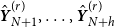




In step 2, both in-sample data and predicted data are used for two reasons. First, the forecast horizon is not too long compared to the in-sample horizon. If only predicted data are used, the extracted factors may not be accurate. Second, incorporating the true trajectories into the reconstruction produces a more stable representation.
7. Data
In this paper, we focus on examining the relative spreads of seven countries/regions (the UK, Germany, France, Italy, Japan, Australia, and the European Union) with respect to US bond yields, which serve as the reference yield. The data used in this analysis consist of monthly data from January 2010 to December 2020.Footnote 3 We use the first ten years as in-sample data to estimate unknown parameters and hidden state variables, and the data for the last year for out-of-sample forecasting.
The original data contain the following maturities:
-
• United States (US): with maturities 1, 3, 6 months, and 1, 2, 3, 5, 7, 10, and 30 years.
-
• United Kingdom (UK): with maturities 1, 3, 6 months, 1, 2, 3, 5, 10, 20, and 30 years.
-
• Germany (DE): with maturities 3, 6, 9 months, and 1, 2, 3, 5, 10, 20, and 30 years.
-
• France (FR): with maturities 1, 3, 6, 9 months, and 2, 3, 5, 10, 20, and 30 years.
-
• Italy (IT): with maturities 6, 9 months, and 2, 3, 5, 10, and 30 years.
-
• Japan (JP): with maturities 6 months, and 1, 2, 3, 5, 10, 20, and 30 years.
-
• Australia (AU): with maturities 1, 2, 3, 5, and 10 years.
-
• European Union (EU): with maturities 1, 3, 6, 9 months, 1, 2, 3, 5, 7, 10, 20, and 30 years.
To provide a better interpretation, we match each country’s maturities to 1, 3, 6, 9 months, 1, 2, 3, 5, 7, 10, 20, and 30 years. For countries/regions without all these maturities, we estimated the missing maturities using the static Nelson–Siegel model:
 \begin{align} Y_t(\tau _i) = F_{1,t} + F_{2,t} \left ( \frac {1 - e^{-\lambda \tau _i}}{\lambda \tau _i} \right ) + F_{3,t} \left ( \frac {1 - e^{-\lambda \tau _i}}{\lambda \tau _i} - e^{-\lambda \tau _i} \right ) + v_t(\tau _i), \end{align}
where $F_{1,t}$
,
$F_{1,t}$
, $F_{2,t}$
, and
$F_{2,t}$
, and $F_{3,t}$
are hidden factors representing the level, slope, and curvature. The difference between Equation (47) and the DNS model described in Section 3.1 is that for Equation (47), we do not assume any dynamics of the factors
$F_{3,t}$
are hidden factors representing the level, slope, and curvature. The difference between Equation (47) and the DNS model described in Section 3.1 is that for Equation (47), we do not assume any dynamics of the factors $F_{i,t}$
, for
$F_{i,t}$
, for $i \in \{ 1,2,3 \}$
. Instead, they are estimated day by day using the least squares method. Figure 2 shows the UK yield curves for the original data and the data after maturity matching, respectively. The 9-month and 7-year bond yields are interpolated in the right sub-figure. Additionally, all missing values are replaced by interpolated values.
$i \in \{ 1,2,3 \}$
. Instead, they are estimated day by day using the least squares method. Figure 2 shows the UK yield curves for the original data and the data after maturity matching, respectively. The 9-month and 7-year bond yields are interpolated in the right sub-figure. Additionally, all missing values are replaced by interpolated values.
UK yield curves from January 2010 to December 2020. The left figure is for the original data, and the right figure is for the data after maturity matching. 9-month yield and 7-year (84-month) yield are interpolated in the right figure.

8. Empirical analysis
In this section, we present the empirical results. We first show the in-sample estimations using the DNS model and the DNS-FR model in Sections 8.1 and 8.2, respectively. Section 8.3 gives the out-of-sample forecasting. To assess the potential issue of overfitting, we compare the functional regression model with a simple addition model in Section 8.4. Then, we test the performance of the DNS-FR model under a permanent shock and a temporary shock in Section 8.5. Finally, one application of the DNS-FR model in the construction of a bond ladder portfolio for risk management is given in Section 8.6.
8.1 Dynamic Nelson–Siegel model
We first present the estimation results of the DNS model, which serves as a benchmark. Model parameters and hidden state variables are jointly estimated by maximizing the marginal likelihood function described in Section 5.3. In this paper, $\lambda$
is fixed at 0.0609, as in Diebold and Li (Reference Diebold and Li2006).
$\lambda$
is fixed at 0.0609, as in Diebold and Li (Reference Diebold and Li2006).
The in-sample Root Mean Squared Error (RMSE) using covariance structure 2 is provided in Table 1. The in-sample RMSE for the DNS model using covariance structures 1 and 3 is given in Appendix B. We first discuss the differences between these covariance structures, as outlined in Section 4. Overall, the differences in mean RMSE are minimal. For long-end maturities, specifically 20-year and 30-year maturities, covariance structure 3 provides the most accurate estimation. However, for short-end and middle maturities, covariance structure 3 exhibits the highest RMSE. It also has the highest mean RMSE for most countries/regions, except Japan. Therefore, covariance structure 3 is not the best choice for this study. Covariance structures 1 and 2 are more evenly matched, with structure 2 outperforming structure 1 for some countries/regions and vice versa. Considering that covariance structure 2 shows some dependencies between yields with different maturities, which is more realistic in the bond market, while structure 1 assumes all yields are uncorrelated, we choose to use structure 2 for further analysis.
In-sample RMSE for DNS model using covariance structure 2

Table 1 Long description
A table with 11 rows and 9 columns comparing in-sample Root Mean Squared Error (RMSE) for DNS model using covariance structure 2 across different regions and maturities. The columns are labeled as Maturity, UK, FR, IT, DE, JP, AU, EU, and US. The rows are labeled with different maturities ranging from 1 month to 30 years, and a mean value. Row 1: Maturity, 1 month, 0.1313, 0.1139, 0.0288, 0.0047, 2.26e-05, 0.0048, 0.1984, 0.0645. Row 2: Maturity, 3 months, 0.0212, 0.0755, 0.0007, 0.0571, 3.20e-15, 0.0005, 0.1307, 0.0126. Row 3: Maturity, 6 months, 0.1027, 0.0449, 0.0679, 0.0677, 0.0323, 0.0026, 0.0492, 0.0688. Row 4: Maturity, 9 months, 0.0511, 0.0738, 0.0722, 0.0891, 0.0071, 0.0012, 0.0590, 0.0324. Row 5: Maturity, 1 year, 0.0999, 0.0142, 3.64e-13, 0.1009, 0.0160, 0.0106, 0.0867, 0.0752. Row 6: Maturity, 2 years, 0.0102, 0.0725, 0.1096, 0.0210, 0.0144, 0.0272, 0.0145, 0.0179. Row 7: Maturity, 3 years, 0.1223, 0.1770, 0.2409, 0.1216, 0.0195, 0.0589, 0.1305, 0.1082. Row 8: Maturity, 5 years, 0.2390, 0.2764, 0.3754, 0.1658, 0.0268, 0.0217, 0.2097, 0.1263. Row 9: Maturity, 7 years, 0.1563, 0.2023, 0.3206, 0.0950, 0.1574, 0.0957, 0.2067, 0.0787. Row 10: Maturity, 10 years, 0.1374, 0.1716, 0.2214, 0.1607, 0.3325, 0.2469, 0.0904, 0.1598. Row 11: Maturity, 20 years, 0.4039, 0.3410, 0.0532, 0.4377, 0.9466, 0.6271, 0.2843, 0.3872. Row 12: Maturity, 30 years, 0.4706, 0.4769, 0.1233, 0.4846, 1.1036, 0.8269, 0.3049, 0.5018. Row 13: Maturity, Mean, 0.1622, 0.1700, 0.1345, 0.1505, 0.2214, 0.1603, 0.1471, 0.1361.
Focusing on covariance structure 2, most countries/regions exhibit a high RMSE for long-end maturities, with the exception of Italy. Italy has a low RMSE for long-end maturities but a high RMSE for middle maturities, between 3 years and 10 years. Similar patterns are observed for the UK, France, and the European Union, which also show high RMSEs for middle maturities. Conversely, the DNS model fits the short-end maturities well across all countries/regions.
These results suggest that while the DNS model generally captures the dynamics well for short-end maturities, it struggles with accuracy at longer maturities for most countries/regions. This discrepancy is likely due to the higher volatility and risk associated with longer-term bonds, which are not fully captured by the DNS model.
Another notable observation is the presence of extremely small values in Tables 1 and 2, in the order of less than 1e-10. This phenomenon can be explained from two perspectives. First, as discussed in Section 7, data for some countries lack certain yield curve maturities used in the analysis. These missing maturities include 9-month and 20-year maturities for the US; 9-month and 7-year maturities for the UK; 1-month and 7-year maturities for Germany; 1-year and 7-year maturities for France; 1-month, 3-month, and 1-year, 7-year, and 20-year maturities for Italy; 1-month, 3-month, 9-month, and 7-year maturities for Japan; and 1-month, 3-month, 6-month, 9-month, and 7-year, 20-year, and 30-year maturities for Australia. These missing maturities are bootstrapped with small observation errors, leading to lower estimation errors for some of these maturities. Second, there are no constraints on the error terms in Equations (24) and (25). Due to the nature of the state-space model, a higher estimated signal-to-noise ratio results in smaller estimation errors for observations. This also explains the presence of extremely small values in some cases.
In-sample RMSE for DNS-FR model with 3 factors using covariance structure 2

Table 2 Long description
The table presents in-sample RMSE values for the DNS-FR model with 3 factors using covariance structure 2. It includes data for various countries (UK, FR, IT, DE, JP, AU, EU) across different maturities (1 month, 3 months, 6 months, 9 months, 1 year, 2 years, 3 years, 5 years, 7 years, 10 years, 20 years, 30 years) and a mean value. The table has 13 rows and 8 columns. Column headers are Maturity, UK, FR, IT, DE, JP, AU, and EU. Row labels include specific maturities and a mean value. Each cell contains a numerical value representing the RMSE for the corresponding country and maturity. Notable trends include varying RMSE values across different countries and maturities, with some extremely small values present.
8.2 DNS-FR model
In this section, we present the estimation results of the DNS-FR model. To estimate the yields of response countries, we first extract factors from US Treasury yields using kPCA as discussed in Section 4. The estimated hyperparameter for the RBF kernel is $\iota = 0.083$
. After extracting these factors, we estimate the yields using the same methodology as the DNS model.
$\iota = 0.083$
. After extracting these factors, we estimate the yields using the same methodology as the DNS model.
We select 3 kPCA factors for this study. Compared to the RMSE using 2 factors, the in-sample RMSE with 3 factors shows significant improvement, particularly for UK yields. Increasing the number of factors to 4 or 5 further reduces the RMSE for most countries/regions, but the improvement is marginal. Given the substantial increase in parameter space and associated computational challenges, we determine that 3 factors strike the optimal balance. Similar to the DNS model, the choice among the three covariance structures shows minimal difference. For consistency, we use covariance structure 2 for the remainder of this paper.
Table 2 presents the in-sample RMSE for the DNS-FR model with 3 factors and covariance structure 2. The in-sample RMSE for other covariance structures and factor counts is provided in Appendix C. The DNS-FR model significantly reduces the mean RMSE compared to the DNS model across all countries/regions. Specifically, for the UK, France, Germany, and European Union yields, the DNS-FR model outperforms the DNS model at all maturities. For Italy yields, while the DNS model shows lower RMSE at 3-month, 1-year, and 30-year maturities, the differences are minimal. For other maturities, the DNS-FR model performs better. For Japan yields, the DNS model has a slight advantage at 1-month and 3-month maturities, whereas for Australia yields, it is more accurate at 9-month, 1-year, and 2-year maturities. Otherwise, the DNS-FR model provides superior yield estimates.
As discussed in Section 8.1, the DNS model struggles with accurately estimating the yield curve for 20-year and 30-year maturities. The DNS-FR model significantly improves this issue. For UK and European Union yields, the RMSE magnitude for long-end maturities aligns closely with other maturities. The DNS model already provides accurate long-end maturity estimates for Italian yields, so the DNS-FR model does not offer much improvement here. For France, Germany, Japan, and Australia yields, the RMSE for long-end maturities remains high, but the DNS-FR model still achieves significant reductions.
For the remainder of this paper, we focus on UK yields, as the DNS-FR model performs well for both short and long maturities.
We close this subsection by discussing the structure of the yield curve. Typically, in the bond market, the yield curve is in an upward-sloping or normal shape, where short-term interest rates are lower than long-term rates due to the higher risk associated with long-term debt. However, under certain conditions, this relationship can invert, leading to an inverted yield curve where long-term bonds have lower yields than short-term bonds. Such inversions are relatively rare and noteworthy as it often indicates an unusual economic environment. Therefore, it is essential to test if models can accurately estimate yield curves in both normal and inverted configurations.
Figure 3 illustrates the estimated UK yield curves by the DNS and DNS-FR models for January 2011, August 2015, and September 2019. In January 2011, the yield curve displayed a normal upward-sloping shape. For bonds with maturities less than 120 months, both models perform similarly. However, for longer maturities, the DNS-FR model provides better estimates. In August 2015, when the curve remained in a normal shape, the DNS-FR model continued to outperform, especially for long-term bonds. Moreover, the DNS-FR model captures short-term fluctuations accurately, whereas the DNS model offers a smoothed estimation. In September 2019, the yield curve exhibited an inversion for maturities less than 60 months, before reverting to a normal slope for longer maturities. The DNS-FR model again demonstrates superior performance, accurately fitting both the inverted and normal segments of the curve.
Estimated UK yield curves by DNS model and DNS-FR model for three different months.

Figure 3 Long description
Three line graphs depict estimated UK yield curves by DNS model and DNS-FR model for three different months. Panel A: A line graph shows the yield curves for January 2011. The x-axis represents maturity in months ranging from 0 to 400, and the y-axis represents yield ranging from 0 to 4.5. The graph includes three lines: Original data, DNS estimation, and DNS-FR estimation. The lines show an upward trend with increasing maturity, with the DNS-FR estimation closely following the original data. Panel B: A line graph shows the yield curves for August 2015. The x-axis represents maturity in months ranging from 0 to 400, and the y-axis represents yield ranging from 0 to 3. The graph includes three lines: Original data, DNS estimation, and DNS-FR estimation. The lines show an upward trend with increasing maturity, with the DNS-FR estimation closely following the original data. An inset zooms in on the 0 to 20 months range. Panel C: A line graph shows the yield curves for September 2019. The x-axis represents maturity in months ranging from 0 to 400, and the y-axis represents yield ranging from 0.2 to 1.2. The graph includes three lines: Original data, DNS estimation, and DNS-FR estimation. The lines show a complex trend with a dip around 50 months and an upward trend beyond 150 months, with the DNS-FR estimation closely following the original data.
Figure 4 presents the extracted kPCA factors $U_{tj}$
(left) and their corresponding coefficients
$U_{tj}$
(left) and their corresponding coefficients $\gamma _{i,j}$
in Equation (22).
$\gamma _{i,j}$
in Equation (22).
Extracted kPCA factors and the corresponding coefficients.

8.3 Forecasting
In this section, we compare the performance of the DNS model and the DNS-FR model in out-of-sample forecasting, using the methods discussed in Section 6. Forecast accuracy is evaluated using the RMSE for 12-step ahead ( $h=12$
) forecasts.
$h=12$
) forecasts.
Tables 3 and 4 present the RMSE for the DNS model and the DNS-FR model, respectively. Interestingly, for all countries/regions, the DNS model provides a lower mean RMSE than the DNS-FR model. However, it is important to recall that, in the DNS-FR model forecasting process described in Section 6, we first forecast the yields of the reference country (US Treasury) using the DNS model. In Table 3, the mean RMSE for the US Treasury yield prediction is notably high, at least double that of the mean RMSE for other countries/regions. Consequently, the reconstructed factors $\hat {\boldsymbol{U}}_{N+1}, \dots , \hat {\boldsymbol{U}}_{N+h}$
may not accurately reflect the US Treasury market during this period.
$\hat {\boldsymbol{U}}_{N+1}, \dots , \hat {\boldsymbol{U}}_{N+h}$
may not accurately reflect the US Treasury market during this period.
12-step ahead forecasting RMSE for the DNS model

Table 3 Long description
A table comparing RMSE values for the DNS model across different regions and maturities. The table has 12 rows and 9 columns. The columns are labeled as Maturity, UK, FR, IT, DE, JP, AU, EU, and US. The rows are labeled with different maturity periods ranging from 1 month to 30 years, plus a mean row. Row 1: Maturity, 1 month, 0.6645, 0.1348, 0.2305, 0.0698, 0.0639, 0.5642, 0.1164, 1.5016. Row 2: Maturity, 3 months, 0.6158, 0.0543, 0.2390, 0.0687, 0.0585, 0.5202, 0.0574, 1.4229. Row 3: Maturity, 6 months, 0.5456, 0.0724, 0.2657, 0.1169, 0.0510, 0.4678, 0.0796, 1.3378. Row 4: Maturity, 9 months, 0.5257, 0.0969, 0.2817, 0.1718, 0.0435, 0.4285, 0.1203, 1.2959. Row 5: Maturity, 1 year, 0.4797, 0.0662, 0.3215, 0.2097, 0.0346, 0.4075, 0.1537, 1.2309. Row 6: Maturity, 2 years, 0.4659, 0.0541, 0.4272, 0.1702, 0.0317, 0.3174, 0.0994, 1.1570. Row 7: Maturity, 3 years, 0.4744, 0.1127, 0.5100, 0.1073, 0.0350, 0.3259, 0.0652, 1.1464. Row 8: Maturity, 5 years, 0.5096, 0.2305, 0.5819, 0.0721, 0.0356, 0.2357, 0.1444, 1.1109. Row 9: Maturity, 7 years, 0.4605, 0.2481, 0.6054, 0.0970, 0.0558, 0.1184, 0.2012, 0.9822. Row 10: Maturity, 10 years, 0.3946, 0.1886, 0.5505, 0.0783, 0.1137, 0.1576, 0.1798, 0.8818. Row 11: Maturity, 20 years, 0.1243, 0.1984, 0.4190, 0.1188, 0.4541, 0.8816, 0.1665, 0.5196. Row 12: Maturity, 30 years, 0.1224, 0.3753, 0.4180, 0.2515, 0.6326, 1.3228, 0.1251, 0.3364. Row 13: Maturity, Mean, 0.4486, 0.1527, 0.4042, 0.1277, 0.1342, 0.4790, 0.1258, 1.0770.
12-step ahead forecasting RMSE for the DNS-FR model

Table 4 Long description
The table presents RMSE values for the DNS model across various countries and regions. It includes data for different maturity periods ranging from 1 month to 30 years. The table has 12 rows and 9 columns. The columns are labeled as Maturity, UK, FR, IT, DE, JP, AU, and EU. The row labels indicate the maturity periods. Each cell contains a numerical value representing the RMSE for the corresponding country and maturity period. The mean RMSE values for each country are also provided at the bottom of the table.
To further compare the performance of the DNS model and the DNS-FR model, we conduct a moving window analysis. The moving window is set as follows: we start with a 5-year window from January 2010 to December 2014, treating this period as in-sample data to estimate model parameters and hidden state variables. We then estimate the yields and calculate the mean RMSE over all maturities and data points within this window. Next, we forecast the yields 12 steps ahead, treating the next 12 months (i.e., from January 2015 to December 2015) as out-of-sample data, and calculate the mean RMSE. We then shift the window forward by one month (i.e., one data point) and repeat the calculations, continuing this process until the last available data point.
Figure 5 shows the in-sample (left) and out-of-sample (right) mean RMSE for UK yields using a moving window. The blue curve represents the mean RMSE for the DNS model, while the red curve represents the mean RMSE for the DNS-FR model. The date of each point corresponds to the midpoint of the window. From the in-sample estimation, it is evident that the DNS-FR model consistently outperforms the DNS model over the entire sample period from 1998 to 2016, with the performance gap widening after 2010. In contrast, for the out-of-sample forecasting, the two curves frequently intersect. During certain periods, such as around 2018, the DNS-FR model achieves a lower mean RMSE, whereas in other periods, notably between 2010 and 2014, the DNS model performs better. Additionally, the differences between the two curves are limited, indicating that both models have similar forecasting performance. The same figures for other countries/regions are provided in Appendix D, and similar conclusions are drawn for all other countries/regions.
In-sample and out-of-sample mean RMSE for UK yields using a 5-year moving window, move forward for 1 month each time. Each point corresponds to the midpoint of the window, with RMSE averaged over the full window.

8.4 Assessing overfitting in the DNS-FR model
In Sections 8.1, 8.2, and 8.3, we demonstrate that the DNS-FR model outperforms the DNS model in in-sample estimation. However, for out-of-sample prediction, the DNS-FR model exhibits only comparable predictive power in some countries. This raises concerns about potential overfitting. In this section, we address this issue by comparing the DNS-FR model with the following model:
 \begin{align} Y_t(\tau _i) & = F_{1,t} + F_{2,t} \left ( \frac {1 - e^{-\lambda \tau _i}}{\lambda \tau _i} \right ) + F_{3,t} \left ( \frac {1 - e^{-\lambda \tau _i}}{\lambda \tau _i} - e^{-\lambda \tau _i} \right ) + \unicode{x03B2} _{\tilde {\tau }} Y_t^{(r)}(\tilde {\tau }) + \epsilon _t(\tau _i) \\[-28pt] \nonumber \end{align}
 \begin{align} F_{j,t} & = \psi _{j,0} + \psi _{j,1} F_{j, t-1} + \unicode{x03B7} _{j, t}. \\[0pt] \nonumber \end{align}
Here, $Y_t^{(r)}(\tilde {\tau })$
denotes the bond yield of the reference country for a given maturity
$Y_t^{(r)}(\tilde {\tau })$
denotes the bond yield of the reference country for a given maturity $\tilde {\tau }$
, and
$\tilde {\tau }$
, and $\unicode{x03B2} _{\tilde {\tau }}$
is the corresponding coefficient. Unlike the DNS-FR model, Equations (48) and (49) do not incorporate a functional component. Instead, they assume that a simple addition of the reference country’s bond yield enhances the DNS model. We refer to this model as the DNS-Reg
$\unicode{x03B2} _{\tilde {\tau }}$
is the corresponding coefficient. Unlike the DNS-FR model, Equations (48) and (49) do not incorporate a functional component. Instead, they assume that a simple addition of the reference country’s bond yield enhances the DNS model. We refer to this model as the DNS-Reg $X$
model, where
$X$
model, where $X$
represents the maturity (in months) of the reference bond yield.
$X$
represents the maturity (in months) of the reference bond yield.
Tables E.1 to E.4 in Appendix E present the in-sample estimation errors and out-of-sample forecasting errors. The response yield is the UK bond yield, while the reference yield is the US Treasury yield at six maturities: 1 month, 12 months, 24 months, 60 months, 120 months, and 360 months. We also compare the DNS-FR model with different numbers of factors (shown in brackets) extracted.
Table D.1 reports the in-sample estimation errors across different models. Incorporating a single US Treasury maturity into the DNS model reduces the RMSE, with longer maturities offering greater improvements in estimating UK bond yields. However, all variations of the DNS-Reg $X$
model yield higher RMSEs than the DNS-FR model, particularly for middle and long-term maturities. This is because the kPCA decomposition captures the level, slope, and curvature dynamics of the US Treasury yield curve, whereas a single time series of US Treasury yields cannot fully represent these features. As a result, although adding a single US Treasury maturity improves the estimation, the functional regression component remains crucial for achieving superior performance. Increasing the number of kPCA factors from 3 to 6 has only a limited impact on in-sample accuracy. For the DNS-FR model with 6 factors, the mean RMSE is 0.0655, approximately 60% lower than that of the DNS model and 37% lower than that of the DNS-Reg360 model.
$X$
model yield higher RMSEs than the DNS-FR model, particularly for middle and long-term maturities. This is because the kPCA decomposition captures the level, slope, and curvature dynamics of the US Treasury yield curve, whereas a single time series of US Treasury yields cannot fully represent these features. As a result, although adding a single US Treasury maturity improves the estimation, the functional regression component remains crucial for achieving superior performance. Increasing the number of kPCA factors from 3 to 6 has only a limited impact on in-sample accuracy. For the DNS-FR model with 6 factors, the mean RMSE is 0.0655, approximately 60% lower than that of the DNS model and 37% lower than that of the DNS-Reg360 model.
For out-of-sample forecasting, we consider three settings: a rolling window of 1-step ahead forecasting over the next 12 months (Table D.2), 2-step ahead forecasting (Table D.3), and 12-step ahead forecasting (Table D.4). Overall, the DNS-FR model outperforms both the DNS and DNS-Reg $X$
models over longer horizons, while DNS-Reg
$X$
models over longer horizons, while DNS-Reg $X$
models achieve lower RMSEs in the short term. For 1-step ahead forecasting, the DNS-Reg120 model achieves the lowest RMSE of 0.1411. In contrast, the best-performing DNS-FR specification, which uses 4 factors, yields an RMSE of 0.1923, around 20% higher than that of the DNS model and 36% higher than the DNS-Reg120 model. This indicates that the functional regression model has limited predictive power over short horizons.
$X$
models achieve lower RMSEs in the short term. For 1-step ahead forecasting, the DNS-Reg120 model achieves the lowest RMSE of 0.1411. In contrast, the best-performing DNS-FR specification, which uses 4 factors, yields an RMSE of 0.1923, around 20% higher than that of the DNS model and 36% higher than the DNS-Reg120 model. This indicates that the functional regression model has limited predictive power over short horizons.
However, for 2-step and 12-step ahead forecasting, the DNS-FR model demonstrates strong predictive performance. In the 2-step ahead setting, the DNS-FR model with 5 factors performs best, with an RMSE of 0.2038, 25% lower than that of the DNS model (0.2709) and 3% lower than the DNS-Reg360 model (0.2108). In the 12-step ahead setting, the best-performing model is the DNS-FR with 6 factors, achieving an RMSE of 0.3275, which is approximately 27% lower than the DNS model and 14% lower than the DNS-Reg360 model. Although the DNS-FR model with 3 factors yields higher forecasting errors than the DNS and DNS-Reg $X$
models, increasing the number of kPCA factors leads to substantial improvements in forecasting accuracy over longer horizons, including 2-step forecasts. This suggests that the DNS-FR model does not suffer from overfitting when applied to UK bond yield data.
$X$
models, increasing the number of kPCA factors leads to substantial improvements in forecasting accuracy over longer horizons, including 2-step forecasts. This suggests that the DNS-FR model does not suffer from overfitting when applied to UK bond yield data.
Figure 6 presents the RMSE of 12-step-ahead forecasts for each tenor of UK bond yields. A 5-year moving window (beginning in January 2010) is employed to fit the model, with the window advancing by one month at each iteration. RMSE values are computed across all windows for each forecast step. For the 2-, 3-, 5-, and 7-year maturities, the DNS-FR model with six factors consistently outperforms the other two models across all forecast steps. In contrast, for the 1-month, 3-month, and 10-year maturities, the DNS-FR model exhibits a larger RMSE than the DNS and DNS-Reg360 models only at a few forecast steps. For the 6-month, 9-month, and 1-year maturities, performance varies across the models. At some steps, the DNS-FR model performs better, while at other steps, the DNS and DNS-Reg360 models yield superior forecasts. For the 20-year and 30-year maturities, the DNS-FR model underperforms relative to the DNS-Reg360 model but achieves a lower RMSE than the DNS model.
RMSE of 5-year moving window for out-of-sample prediction over 12 steps for each tenor of UK bond yields. The window moves forward for 1 month each time. Results are shown for the DNS model (green), DNS-Reg360 model (blue), and DNS-FR model with 6 factors (red).

Figure 6 Long description
The image contains twelve line graphs labeled from (a) to (l), each representing the RMSE of out-of-sample predictions for UK bond yields over 12 steps for different maturities. Each graph compares the performance of three models: DNS model (green), DNS-Reg360 model (blue), and DNS-FR model with 6 factors (red). The x-axis of each graph represents the step number, ranging from 0 to 12, while the y-axis represents the RMSE values. Panel (a) shows the RMSE for 1 month maturity, Panel (b) for 3 months maturity, Panel (c) for 6 months maturity, Panel (d) for 9 months maturity, Panel (e) for 1 year maturity, Panel (f) for 2 years maturity, Panel (g) for 3 years maturity, Panel (h) for 5 years maturity, Panel (i) for 7 years maturity, Panel (j) for 10 years maturity, Panel (k) for 20 years maturity, and Panel (l) for 30 years maturity. Each graph shows the RMSE values fluctuating across the steps, with varying trends and patterns for each model and maturity.
Figure 7 displays the mean RMSE across all tenors for the three models. The DNS-FR model with six factors consistently achieves the smallest mean RMSE across all forecast steps, while the DNS model records the largest. The DNS-Reg360 model performs better than the DNS model but still exhibits a larger mean RMSE than the DNS-FR model.
Mean RMSE of 5-year moving window for out-of-sample prediction. The mean value is taken over all maturities.

In the remainder of this paper, we focus on the DNS-FR model with 3 factors, despite the 6-factor model demonstrating superior predictive accuracy. This choice is motivated by the fact that the 3-factor model achieves comparable in-sample estimation accuracy while involving significantly fewer parameters.
8.5 Stress testing
In this section, we conduct a stress testing analysis to answer the following question: If different shocks are applied to the US Treasury market, how do the bond markets of other countries/regions respond? We define two types of stress testing scenarios, each with four cases:
-
• Scenario 1: Temporary shocks (January 2015 to December 2015).
-
– Case 1.1: Short-end maturities (1, 3, 6, 9 months, and 1, 2, 3, 5 years) yield double.
-
– Case 1.2: Middle maturities (7 and 10 years) yield double.
-
– Case 1.3: Long-end maturities (20 and 30 years) yield double.
-
– Case 1.4: Entire yield curve doubles.
-
-
• Scenario 2: Permanent shocks (beginning January 2015).
-
– Case 2.1: Short-end maturities (1, 3, 6, 9 months, and 1, 2, 3, 5 years) yield double.
-
– Case 2.2: Middle maturities (7 and 10 years) yield double.
-
– Case 2.3: Long-end maturities (20 and 30 years) yield double.
-
– Case 2.4: Entire yield curve doubles.
-
To estimate the yields of the response countries, we first apply each stress testing scenario to the US Treasury yield curve. The time series of the US Treasury yields under different stress testing scenarios is provided in Appendix F. Using the amended US Treasury data, we extract kPCA factors. For consistency, we use three factors in this study, with the estimated hyperparameter $\iota$
for each scenario listed in Table 5. Finally, we estimate the yields of the response countries.
$\iota$
for each scenario listed in Table 5. Finally, we estimate the yields of the response countries.
Estimated hyperparameter $\iota$
using 3 factors for different stress testing cases
$\iota$
using 3 factors for different stress testing cases

Table 5 Long description
A table titled Estimated hyperparameter using 3 factors for different stress testing cases. The table has two columns: Stress testing cases and Estimated hyperparameter. It contains 11 rows, including a header row. Row 1: Original data, 0.083. Row 2: Stress testing 1, case 1.1, 0.091. Row 3: Stress testing 1, case 1.2, 0.080. Row 4: Stress testing 1, case 1.3, 0.115. Row 5: Stress testing 1, case 1.4, 0.081. Row 6: Stress testing 2, case 2.1, 0.059. Row 7: Stress testing 2, case 2.2, 0.096. Row 8: Stress testing 2, case 2.3, 0.183. Row 9: Stress testing 2, case 2.4, 0.037.
Figures 8 and 9 show the mean difference in in-sample estimation for UK yields under temporary and permanent shock scenarios, respectively, compared to the estimation under original US Treasury data. Each sub-figure corresponds to cases 1.1 to 1.4 and 2.1 to 2.4. We categorize bonds into three classes: short-end ( $(0, 5]$
years), middle (
$(0, 5]$
years), middle ( $(5, 10]$
years), and long-end (
$(5, 10]$
years), and long-end ( $(10, 30]$
years). The mean value is taken over all maturities in each class at each time point. The dashed lines represent the lower and upper bounds of the 95% confidence interval,Footnote 4 while the vertical black lines indicate the start and end of the shock period for the temporary shocks.
$(10, 30]$
years). The mean value is taken over all maturities in each class at each time point. The dashed lines represent the lower and upper bounds of the 95% confidence interval,Footnote 4 while the vertical black lines indicate the start and end of the shock period for the temporary shocks.
We first consider the effects of the temporary shocks in Figure 8. When the shock is applied to the short-end maturities of the US Treasury yield curve (case 1.1), the effect on UK yields is limited. The confidence intervals cover 0 at almost all time points for all three classes. The short-end maturities of UK yields may have some changes during the shock, but will return to normal levels once the shock ends. When the shock is applied to the middle maturities of the US Treasury (case 1.2), there is a statistically significant effect on the short-end and middle maturities of UK yields. The long-end maturities of UK yields are not affected. Interestingly, even though the shock ended in December 2015, the effects persist in the long run. In case 1.3, when the shock is applied to the long-end maturities of the US Treasury, the entire yield curve is affected, but the long-end maturities are most impacted. Even after the shock, the mean differences in the estimation of long-end maturities remain significantly away from 0. Finally, in case 1.4, when the shock is applied to the entire US Treasury yield curve, the mean differences in the estimation of middle maturities of UK yields are affected in some intervals, for example, from July 2015 to September 2016, and from September 2017 to December 2019, while neither the short nor the long maturities exhibit a significant effect.
Mean difference in percentage points of in-sample estimations between stress testing scenario 1 and original data for UK yields. The mean values are taken over short-end ( $(0, 5]$
years), middle (
$(0, 5]$
years), middle ( $(5, 10]$
years), and long-end (
$(5, 10]$
years), and long-end ( $(10, 30]$
years) maturities. Dashed lines represent the lower and upper bounds of 95% confidence interval for each curve.
$(10, 30]$
years) maturities. Dashed lines represent the lower and upper bounds of 95% confidence interval for each curve.

One should note that for the temporary shock, even though it ended in December 2015, some maturities of UK yields are still affected in the long run in some cases, such as the middle maturities in case 1.2 and the long-end maturities in case 1.3. This can be explained as follows. In a regression model, the change in the covariate at time $t$
only affects the response variable at time
$t$
only affects the response variable at time $t$
. However, if the covariate is autoregressive, the change in the covariate at time
$t$
. However, if the covariate is autoregressive, the change in the covariate at time $t$
will be accumulated over a long period.
$t$
will be accumulated over a long period.
Now, we move on to the permanent shock in Figure 9. Unlike the temporary shock, a permanent shock usually does not affect the UK yields in the long run. During the first few months after the shock starts, all the short-end, middle, and long-end maturities of UK yields react to this shock. However, after that, the yield curve returns to normal levels and fluctuates in the short run. The permanent shock affects the middle and long-end maturities more than the short-end maturities in all four cases.
Mean difference in percentage points of in-sample estimations between stress testing scenario 2 and the original data for UK yields. The mean values are taken over short-end ( $(0, 5]$
years), middle (
$(0, 5]$
years), middle ( $(5, 10]$
years), and long-end (
$(5, 10]$
years), and long-end ( $(10, 30]$
years) maturities. Dashed lines represent the lower and upper bounds of 95% confidence interval for each curve.
$(10, 30]$
years) maturities. Dashed lines represent the lower and upper bounds of 95% confidence interval for each curve.

Figure 9 Long description
Four line graphs depict the mean difference in yields for short-end, middle, and long-end maturities of US Treasury bonds under different shock scenarios. Panel A: The line graph shows the mean difference in yields for short-end, middle, and long-end maturities when the shock is applied to the short-end maturities of US Treasury. The x-axis represents the date from 2011 to 2019, and the y-axis represents the mean difference in yields ranging from -0.3 to 0.3. The graph includes three lines representing short-end maturity, middle maturity, and long-end maturity, with dashed lines indicating the lower and upper bounds of the 95% confidence interval for each curve. Panel B: The line graph shows the mean difference in yields for short-end, middle, and long-end maturities when the shock is applied to the middle maturities of US Treasury. The x-axis represents the date from 2011 to 2019, and the y-axis represents the mean difference in yields ranging from -0.4 to 0.4. The graph includes three lines representing short-end maturity, middle maturity, and long-end maturity, with dashed lines indicating the lower and upper bounds of the 95% confidence interval for each curve. Panel C: The line graph shows the mean difference in yields for short-end, middle, and long-end maturities when the shock is applied to the long-end maturities of US Treasury. The x-axis represents the date from 2011 to 2019, and the y-axis represents the mean difference in yields ranging from -0.4 to 0.4. The graph includes three lines representing short-end maturity, middle maturity, and long-end maturity, with dashed lines indicating the lower and upper bounds of the 95% confidence interval for each curve. Panel D: The line graph shows the mean difference in yields for short-end, middle, and long-end maturities when the shock is applied to all maturities of US Treasury. The x-axis represents the date from 2011 to 2019, and the y-axis represents the mean difference in yields ranging from -0.3 to 0.3. The graph includes three lines representing short-end maturity, middle maturity, and long-end maturity, with dashed lines indicating the lower and upper bounds of the 95% confidence interval for each curve.
Another notable feature is the green peaks almost immediately after the shocks start in cases 1.3/2.3 and 1.4/2.4 in Figures 8 and 9. This indicates that whenever a temporary or permanent shock is applied to the long-end maturities or the entire US Treasury yield curve, the long-end maturities of UK bonds react immediately. However, the UK bond market may overreact to this shock. Subsequently, the effects of this shock decrease, and the yields return to normal levels in a few months. If the shock is temporary, when it ends, the UK bond market, especially the long-end maturities, will overreact again. This is because, in our stress testing setup, when a temporary shock ends, the US Treasury yields are halved, causing another dramatic change in the US Treasury yield curve.
Finally, Figure 10 provides the estimated functional coefficients for the UK yields for the original US Treasury data, stress testing scenario 1 data, and stress testing scenario 2 data. For the stress testing data, we only consider cases 1.4 and 2.4, i.e., shocks applied to the entire yield curve. In each sub-figure, different colors represent different functional coefficients $\gamma _i(\tau )$
for
$\gamma _i(\tau )$
for $i \in \{ 1, \dots , 12 \}$
, in Equation (8).
$i \in \{ 1, \dots , 12 \}$
, in Equation (8).
For the original US Treasury data, the long-end maturities of UK bonds are mostly affected by the long-end maturities of the US Treasury ( $\gamma _{11}(\tau ), \gamma _{12}(\tau )$
), while the middle maturities of UK bonds are mostly affected by the middle maturities of the US Treasury (
$\gamma _{11}(\tau ), \gamma _{12}(\tau )$
), while the middle maturities of UK bonds are mostly affected by the middle maturities of the US Treasury ( $\gamma _{9}(\tau ), \gamma _{10}(\tau )$
). All other maturities are evenly affected by the entire US Treasury yield curve. When a temporary shock is applied to the US Treasury, these relationships change slightly. The long-end maturities of UK bonds are still affected by the long-end maturities of the US Treasury, but they are also affected by the 1-year, 2-year, and 3-year US Treasury. The effects of the middle maturities of the US Treasury decrease. All other UK bonds with maturities less than or equal to 10 years are evenly affected by the entire US Treasury yield curve. As for the permanent shock, the effects of the long-end maturities of the US Treasury disappear. Instead, the middle maturities of the US Treasury contribute more to the UK bonds, especially the middle maturities of UK bonds (
$\gamma _{9}(\tau ), \gamma _{10}(\tau )$
). All other maturities are evenly affected by the entire US Treasury yield curve. When a temporary shock is applied to the US Treasury, these relationships change slightly. The long-end maturities of UK bonds are still affected by the long-end maturities of the US Treasury, but they are also affected by the 1-year, 2-year, and 3-year US Treasury. The effects of the middle maturities of the US Treasury decrease. All other UK bonds with maturities less than or equal to 10 years are evenly affected by the entire US Treasury yield curve. As for the permanent shock, the effects of the long-end maturities of the US Treasury disappear. Instead, the middle maturities of the US Treasury contribute more to the UK bonds, especially the middle maturities of UK bonds ( $\gamma _{8}(\tau ), \gamma _{9}(\tau ), \gamma _{10}(\tau )$
).
$\gamma _{8}(\tau ), \gamma _{9}(\tau ), \gamma _{10}(\tau )$
).
Functional coefficients for UK yields.

Construction of a bond ladder portfolio.

8.6 Case study: Bond ladder portfolio
In this section, we present a case study of a bond ladder portfolio for risk management purposes. A bond ladder portfolio can be described as follows. Assume a US investor wants to construct an investment strategy consisting of cash and a UK bond with a maturity of $T$
months. At time
$T$
months. At time $t_i$
, the investor spends
$t_i$
, the investor spends $p_i$
dollars to purchase bonds and deposits the remaining amount in a bank account. We denote the number of bonds as
$p_i$
dollars to purchase bonds and deposits the remaining amount in a bank account. We denote the number of bonds as $N_i$
and the value of the portfolio at time
$N_i$
and the value of the portfolio at time $t_i$
as
$t_i$
as $W_i$
for
$W_i$
for $i \in \{ 0, 1, \dots , k \}$
. The initial wealth
$i \in \{ 0, 1, \dots , k \}$
. The initial wealth $W_0$
is 12 million USD. For simplicity, we assume
$W_0$
is 12 million USD. For simplicity, we assume $p_1 = p_2 = \dots = p$
, meaning the investor spends the same amount on bonds each month. The value of the portfolio
$p_1 = p_2 = \dots = p$
, meaning the investor spends the same amount on bonds each month. The value of the portfolio $W_t$
can be calculated as follows, assuming the interest rate is compounded monthly, and the investment interval is one month:
$W_t$
can be calculated as follows, assuming the interest rate is compounded monthly, and the investment interval is one month:
 \begin{align} W_i = \sum _{j=0}^k N_j F_i e^{-\tau _j Y_i(\tau _j)} \boldsymbol{1}_{\{ t_j \le t_i, \tau _j \ge 0\}} + \left ( 1+\frac {r_i}{12} \right ) C_{i-1} \end{align}
where $F_i$
is the face value in USD at time
$F_i$
is the face value in USD at time $t_i$
,Footnote 5
$t_i$
,Footnote 5 $r_i$
is the risk-free interest rateFootnote 6 for the period
$r_i$
is the risk-free interest rateFootnote 6 for the period $[t_{i-1}, t_{i}]$
,
$[t_{i-1}, t_{i}]$
, $\boldsymbol{1}_{\{ \cdot \}}$
is the indicator function, and
$\boldsymbol{1}_{\{ \cdot \}}$
is the indicator function, and $C_{i-1}$
is the amount in the cash account at time
$C_{i-1}$
is the amount in the cash account at time $t_{i-1}$
. The number of bonds
$t_{i-1}$
. The number of bonds $N_j$
is calculated as:
$N_j$
is calculated as:
 \begin{align} N_j = \frac {p}{F_j e^{-T Y_j(T)}}. \end{align}
Figure 11 illustrates the entire process of constructing the bond ladder portfolio.
Monthly EFFR data and the GBP/USD exchange rate for the year 2020

Table 6 Long description
The table has three columns and thirteen rows. The columns are labeled Date, EFFR, and GBP/USD exchange rate. The rows list data for each month from December 2019 to December 2020. Row 1: Date, Did; EFFR, ; GBP/USD exchange rate, 1.32018. Row 2: Date, January 2020; EFFR, 1.59 percent; GBP/USD exchange rate, 1.28231. Row 3: Date, February 2020; EFFR, 1.59 percent; GBP/USD exchange rate, 1.24086. Row 4: Date, March 2020; EFFR, 0.08 percent; GBP/USD exchange rate, 1.25907. Row 5: Date, April 2020; EFFR, 0.05 percent; GBP/USD exchange rate, 1.23455. Row 6: Date, May 2020; EFFR, 0.05 percent; GBP/USD exchange rate, 1.23992. Row 7: Date, June 2020; EFFR, 0.08 percent; GBP/USD exchange rate, 1.30770. Row 8: Date, July 2020; EFFR, 0.10 percent; GBP/USD exchange rate, 1.33690. Row 9: Date, August 2020; EFFR, 0.09 percent; GBP/USD exchange rate, 1.29115. Row 10: Date, September 2020; EFFR, 0.09 percent; GBP/USD exchange rate, 1.29457. Row 11: Date, October 2020; EFFR, 0.09 percent; GBP/USD exchange rate, 1.33173. Row 12: Date, November 2020; EFFR, 0.09 percent; GBP/USD exchange rate, 1.36561. Row 13: Date, December 2020; EFFR, 0.09 percent; GBP/USD exchange rate, 1.36893.
Predicted portfolio values.

Differences in portfolio values between each stress testing scenario and the original data, for different maturities of the underlying bond.

5% value-at-risk (VaR) for bond ladder portfolios with different maturities.

Differences of 5% value-at-risk (VaR) between each stress testing scenario and the original data, for different maturities of the underlying bond.

Figure 15 Long description
Three line graphs depict the differences in 5% value-at-risk (VaR) for bonds with different maturities under temporary and permanent shocks over a 12-month period. Panel A: A line graph shows the difference in 5% VaR for a 6-month maturity bond. The x-axis represents time in months, ranging from 0 to 12, and the y-axis represents the difference in 5% VaR in dollars, ranging from 0 to -7000. Two lines are plotted: one for temporary shock and one for permanent shock. Both lines show a downward trend, with the permanent shock line consistently lower than the temporary shock line. Panel B: A line graph shows the difference in 5% VaR for a 1-year maturity bond. The x-axis represents time in months, ranging from 0 to 12, and the y-axis represents the difference in 5% VaR in dollars, ranging from 0 to -20000. Two lines are plotted: one for temporary shock and one for permanent shock. The temporary shock line shows a more pronounced downward trend compared to the permanent shock line. Panel C: A line graph shows the difference in 5% VaR for a 30-year maturity bond. The x-axis represents time in months, ranging from 0 to 12, and the y-axis represents the difference in 5% VaR in dollars, ranging from 0 to -1200000. Two lines are plotted: one for temporary shock and one for permanent shock. Both lines show a downward trend, with the permanent shock line consistently lower than the temporary shock line.
In this study, we assume the investor makes 13 investments ( $k+1=13$
) over one year, from December 2019 to December 2020. The effective federal funds rate (EFFR) data and the GBP/USD exchange rateFootnote 7 for this period are given in Table 6. Furthermore, we assume the bond yield for the first investment (made in December 2019) is known, while the yields for the subsequent 12 investments are predicted using the DNS-FR model.Footnote 8 We consider three main questions:
$k+1=13$
) over one year, from December 2019 to December 2020. The effective federal funds rate (EFFR) data and the GBP/USD exchange rateFootnote 7 for this period are given in Table 6. Furthermore, we assume the bond yield for the first investment (made in December 2019) is known, while the yields for the subsequent 12 investments are predicted using the DNS-FR model.Footnote 8 We consider three main questions:
-
1. How does the value of the portfolio change over time?
-
2. How do different stress tests affect the value of the portfolio?
-
3. How does the value of the portfolio change with different maturities of the underlying bond?
For the second question, we consider the stress testing scenarios 1.4 and 2.4 described in Section 8.5, i.e., the shocks are applied to the entire yield curve. For the third question, we consider three different bonds with maturities of 6 months, 1 year, and 30 years, respectively.
Figure 12 shows the predicted portfolio values for the next 12 months for underlying bonds with maturities of 6 months, 1 year, and 30 years. The monthly investment amount is $\$1$
million for all maturities. For the first five months, the portfolio values of all bonds are lower than the initial wealth of
$\$1$
million for all maturities. For the first five months, the portfolio values of all bonds are lower than the initial wealth of $\$12$
million, mainly due to the decrease in the exchange rate. This also explains the decreases in portfolio values in the 8th and 9th months. At the end of 12 months, the 1-year bond has the maximum predicted portfolio value, followed by the 30-year bond, and the 6-month bond has the minimum predicted portfolio value. However, the differences among the three bonds are small. Another notable observation is that as maturities increase, so does risk. For example, at the end of 12 months, the portfolio value of the 6-month bond is roughly
$\$12$
million, mainly due to the decrease in the exchange rate. This also explains the decreases in portfolio values in the 8th and 9th months. At the end of 12 months, the 1-year bond has the maximum predicted portfolio value, followed by the 30-year bond, and the 6-month bond has the minimum predicted portfolio value. However, the differences among the three bonds are small. Another notable observation is that as maturities increase, so does risk. For example, at the end of 12 months, the portfolio value of the 6-month bond is roughly $\$12.5$
million with no uncertainty, while the portfolio value of the 30-year bond could be as high as
$\$12.5$
million with no uncertainty, while the portfolio value of the 30-year bond could be as high as $\$14.5$
million or as low as
$\$14.5$
million or as low as $\$11$
million, reflecting the common understanding that long-term debt usually carries higher risk.
$\$11$
million, reflecting the common understanding that long-term debt usually carries higher risk.
Figure 13 illustrates the differences in portfolio values between different shocks and the original data for the 6-month, 1-year, and 30-year bonds, respectively. A positive value indicates that the portfolio is worth more under the shock, while a negative value indicates that it is worth less. For short-end maturities (6-month and 1-year), the temporary shock has limited effects, but the permanent shock significantly impacts portfolio values. However, for the long-end maturity (30-year), the opposite is true. The permanent shock in 2015 has a larger effect on the portfolio values. Although this shock dissipated by the end of 2015, it continues to affect the long-end curve over an extended period.
In reality, VaR also attracts considerable attention. People are particularly concerned with the maximum potential loss under normal market conditions after excluding the worst outcomes with a total probability of $p\%$
. Figure 14 shows the 5% VaR for the portfolio value of bonds with 6-month, 1-year, and 30-year maturities, which is calculated numerically. At the end of 12 months, the 5% VaR of the portfolio values of the 6-month and 1-year bonds are roughly
$p\%$
. Figure 14 shows the 5% VaR for the portfolio value of bonds with 6-month, 1-year, and 30-year maturities, which is calculated numerically. At the end of 12 months, the 5% VaR of the portfolio values of the 6-month and 1-year bonds are roughly $\$12.5$
and
$\$12.5$
and $\$12.7$
million, respectively, indicating a minimal chance of loss with these bonds even in the worst cases. In contrast, the 5% VaR of the portfolio value of the 30-year bond is only about
$\$12.7$
million, respectively, indicating a minimal chance of loss with these bonds even in the worst cases. In contrast, the 5% VaR of the portfolio value of the 30-year bond is only about $\$11.2$
million, suggesting that investing in a 30-year bond could lead to a loss over a 1-year period in the worst case.
$\$11.2$
million, suggesting that investing in a 30-year bond could lead to a loss over a 1-year period in the worst case.
Figure 15 shows the difference in 5% VaR between each stress testing scenario and the original US Treasury data for different maturities of UK bonds. Overall, if a shock is applied to the US Treasury, the 5% VaR of the portfolio value of UK bonds will decrease. For the 6-month bond, both the temporary shock and the permanent shock have a similar effect on 5% VaR. For the 1-year bond, the permanent shock has a limited effect on 5% VaR, while the temporary shock has a significant influence. For the 30-year bond, both temporary and permanent shocks have a substantial influence on 5% VaR, with the influence of the temporary shock being stronger. Another notable feature is the magnitude of the difference in 5% VaR. For the 6-month bond, a shock can cause a decrease in 5% VaR up to $\$7,000$
at the end of 12 months, while for the 30-year bond, a temporary shock causes a decrease of
$\$7,000$
at the end of 12 months, while for the 30-year bond, a temporary shock causes a decrease of $\$1,200,000$
in 5% VaR. Long-term bonds are more sensitive to the shock.
$\$1,200,000$
in 5% VaR. Long-term bonds are more sensitive to the shock.
9. Conclusion
The DNS model has been pivotal in yield curve estimation over the past two decades. However, it falls short in capturing the relative spread between two economies. In this paper, we introduce a novel DNS-FR model, which extends the DNS model by incorporating the relative spread between a reference country and a response country. To address estimation challenges, we use kPCA to transform the functional regression into a finite-dimensional estimation problem. The Kalman Filter method is then employed to estimate unknown parameters and hidden state variables by maximizing the marginal likelihood function.
Our empirical analysis, which includes eight countries/regions with the US as the reference country and seven response countries/regions, demonstrates that the DNS-FR model outperforms the DNS model in in-sample estimation, particularly for long-term bonds with maturities of 20 and 30 years, across all seven response countries/regions. Additionally, the DNS-FR model is superior in capturing unusual yield curve structures, such as local fluctuations and inversions.
Furthermore, we conducted stress tests to analyze the effects of both temporary and permanent shocks applied to the US Treasury yield curve on the estimation of UK bond yields. The study reveals that middle and long-end maturities of UK bonds are mostly affected, regardless of whether the shock is applied to the short-end, middle, or long-end maturities of the US Treasury yield curve. Interestingly, for temporary shocks, their effects persist in the long run even after the shocks end.
Finally, we conducted a case study of a bond ladder portfolio, involving regular investments in UK bonds for risk management purposes. We forecasted the portfolio values 12 steps ahead with 6-month, 1-year, and 30-year bonds. The predicted portfolio values for the three bonds are similar, but the bond with a longer maturity carries higher risk, reflected in a wider confidence interval. The 5% VaR suggests that investing in the 6-month and 1-year bonds is unlikely to result in a loss over one year, whereas investing in the 30-year bond may lead to a loss in the worst-case scenario. Furthermore, we analyzed the influence of different types of shocks on the predicted portfolio values and VaR. The permanent shock has larger effects on short-end maturities, while the temporary shock, even though it ended a few years ago, has a more significant effect on long-end maturities.
Acknowledgements
This study was partially presented at the 68th Euro Working Group for Commodity and Financial Modelling. We would like to thank the audience and organizers for their valuable feedback and suggestions.
Supplementary material
The supplementary material for this article can be found at https://doi.org/10.1017/S174849952610027X
Data availability statement
The original bond yield data were obtained from https://www.tradingview.com/. The authors do not have permission to share the raw data. A sample data and the codes are available on GitHub at: https://github.com/peilun-he/State-Space-Dynamic-Functional-Regression-for-Multicurve.
Funding statement
This work received no specific grant from any funding agency, commercial, or not-for-profit sectors.
Competing interests
All authors declare that they have no competing interests.
Author contributions
Software: Peilun He; Gareth W. Peters; Nino Kordzakhia. Validation: Peilun He. Investigation: Peilun He; Gareth W. Peters; Nino Kordzakhia; Pavel V. Shevchenko. Formal analysis: Peilun He; Gareth W. Peters. Writing – Original Draft: Peilun He; Gareth W. Peters. Writing – Review and Editing: Peilun He; Gareth W. Peters; Nino Kordzakhia; Pavel V. Shevchenko. Visualization: Peilun He. Conceptualization: Gareth W. Peters. Methodology: Gareth W. Peters; Nino Kordzakhia; Pavel V. Shevchenko. Supervision: Gareth W. Peters; Nino Kordzakhia; Pavel V. Shevchenko.








 λ=0.0609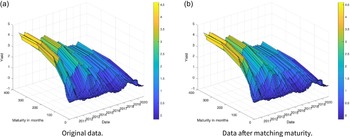
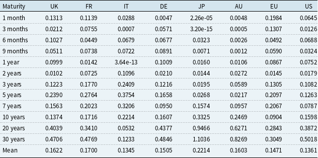
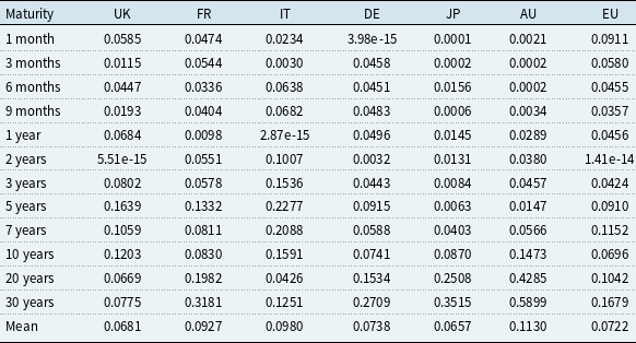
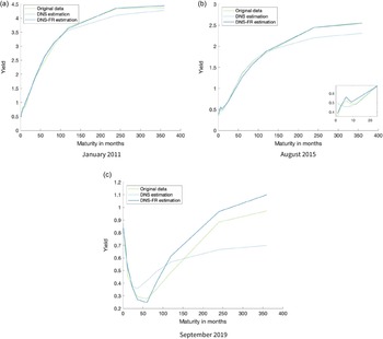

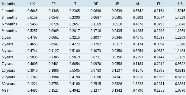
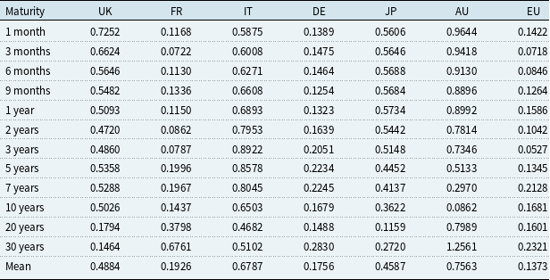


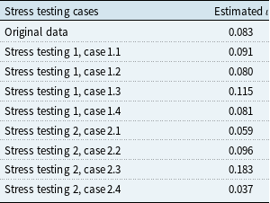
 ι
ι
 (0,5]
(0,5] (5,10]
 (10,30]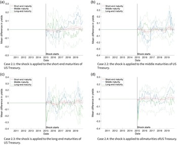
 (0,5]
(0,5] (5,10]
 (10,30]
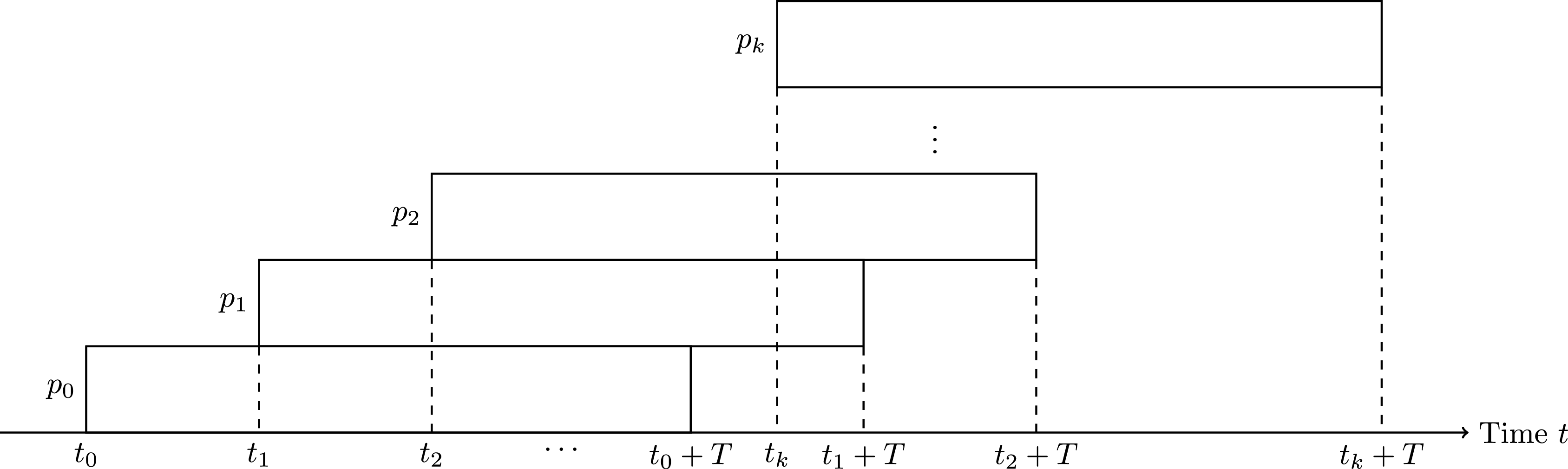
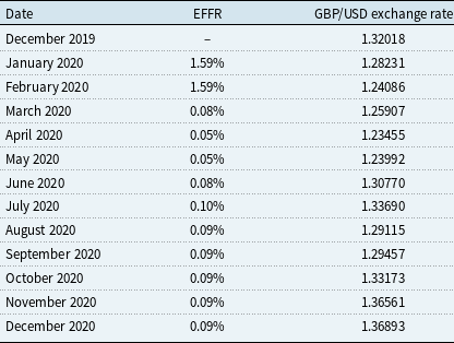


 Open access

