


1. Introduction
How should a Central Bank conduct monetary policy? Should it seek to control some monetary aggregate or should it target some interest rate? Periodically, the Fed has switched its policy targets. Prior to 1979, the Fed generally targeted the federal funds rate. Then, for the brief period 1979–1982 it targeted the narrow monetary aggregate, M1, gradually broadening the target over the period 1982–1993 to include M2, after which Chairman Greenspan announced that the Fed would no longer use monetary aggregates to guide policy. This choice of monetary targets gave rise to the “monetary instrument problem,” originally formulated by Poole (Reference Poole1970), who using a simple stochastic IS-LM model analyzed whether it is preferable to operate monetary policy by targeting the money supply or by controlling the interest rate. Poole’s study spawned an extensive literature, focusing on aspects such as the potential indeterminacy of the price level when pegging the nominal interest rate (Sargent and Wallace (Reference Sargent and Wallace1975), McCallum (Reference McCallum1981)) and the choice of the optimal monetary aggregate to target (Roper and Turnovsky (Reference Roper and Turnovsky1980), Barnett (Reference Barnett1982)).
The early literature focused exclusively on the implications of the choice of monetary policy for aggregate measures, specifically the stability of national income. While this is a natural objective, it is also important to determine the consequences the choice of monetary policy instrument may have for the distribution of wealth and income across heterogeneous agents in the economy. In fact, there is growing literature investigating the relationship between monetary policy and inequality measures, see Colciago et al. (Reference Colciago, Samarina and de Haan2019) for a comprehensive review. As the authors note, many studies are purely empirical and yield conflicting results. The lack of clear conclusion suggests the importance of comparing the distributional consequences of alternative forms of monetary policy within a more structured framework. The objective of this paper is to provide such a framework and to compare the implications for the distribution of wealth and income across heterogeneous agents, when the monetary authority targets the nominal money growth rate versus pegging the nominal interest rate.
While our primary focus is on the monetary instrument problem as articulated by Poole, we also briefly address the related monetary policy of “inflation targeting.” This policy was first introduced by the Reserve Bank of New Zealand in 1989 and has since been adopted by a number of Central Banks. The countries to have introduced some form of inflation targeting include the United Kingdom, the USA, Canada, Sweden, Australia, and South Korea. The target inflation rates are typically around 2% but often allow some flexibility in the range 1–3%.
In choosing the framework to employ for this analysis, two key issues must be addressed. These pertain to: (i) the nature of the heterogeneous agent model and (ii) the degree of money-price flexibility. With respect to the former, our choice is to adopt the “representative consumer theory of distribution” (RCTD) framework originally introduced by Caselli and Ventura (Reference Caselli and Ventura2000).Footnote 1 This approach assumes complete markets and homothetic utility. Its structure facilitates aggregation, with the evolution of the aggregate (macroeconomic) variables and the impact of policy being determined independently of any distributional characteristics. In fact, some support for this approach is provided by Krusell and Smith (Reference Krusell and Smith1998), who suggested that the underlying household wealth and income inequality have only relatively modest impact on the aggregate dynamics. Overall, we view the tractability of the RCTD approach, its amenability to calibration, and its facility to characterize transitional dynamics, as sufficiently appealing so as to adopt it over the more stylized incomplete asset markets approach based on Bewley (Reference Bewley1977) and Aiyagari (Reference Aiyagari1994).
But we also acknowledge that the RCTD approach imposes restrictions, such as the absence of idiosyncratic productivity shocks and limited market accessibility, which are at the heart of the incomplete markets setup. Also, to preserve homothetic utility and to take advantage of the aggregation it facilitates, constrains how money can be introduced into system. These restrictions impact the macro-dynamic equilibrium and have consequences for inequality.
Motivated in part by the doctrine espoused by Friedman (Reference Friedman1960), who long ago advocated the proposition that monetary policy should be directed to maintaining a stable nominal money growth rate, we focus on the long run. Thus, we address the monetary instrument problem in the context of a standard Ramsey model in which agents make their consumption and savings decisions to maximize their intertemporal utility, with prices being assumed to be completely flexible. We adapt the well-known Sidrauski (Reference Sidrauski1967) money-growth model to include heterogeneous agents, whose heterogeneity stems from their differential initial asset endowments. Instead of focusing on the usual aggregates such as the capital stock, employment, and output, we consider the implications for the distributions of wealth and income across agents. The reason for doing so is that in a long-run model such as this, with perfectly flexible prices, the role of monetary policy in influencing long-run real productive elements is limited. But, in contrast, the form of monetary control, by influencing the transitional path of financial variables, does have consequences for the distributions of both wealth and income, over time and in steady state.
Overall, while our choice of analytical framework—RCTD heterogeneity coupled with long-run monetary growth and flexible prices—is clearly restrictive, we nevertheless view it as providing a reasonable benchmark. Moreover, as our results below will confirm, it is compatible with substantial bodies of empirical evidence and can potentially help reconcile some of the conflicting results found in the literature.
Using the above setup, this paper addresses the distributional consequences of two types of changes. The first is a pure expansionary monetary policy. In this case, we find that with perfectly flexible prices, and in the absence of taxes impeding production, monetary policy in isolation has no dynamic consequences. If the central bank, maintaining a constant nominal money growth rate, engages in an expansionary policy by increasing its growth rate, there are no real effects. Instead, it will lead to an immediate increase in the price level leading to an instantaneous portfolio adjustment.Footnote 2 This reduces the share of assets denominated in nominal terms (money and bonds) in the economy, which, being held in greater proportion by the relatively less affluent, causes wealth inequality to immediately increase. But by reducing the real value of bonds and the income it generates, while the real wage rate remains unaffected, the price increase raises the share of income earned by labor, which favors the less affluent. The distribution of income is thus impacted by both these influences, and the net effect on income inequality depends upon which effect dominates. In contrast, if the monetary authority pegging the nominal interest engages in monetary expansion by reducing the interest rate, the price will immediately drop, causing precisely the opposite responses; wealth inequality will decline and the response of income inequality is uncertain.
Numerical simulations suggest that in either case the response of the price level is sensitive to the existing portfolio structure. These simulations also suggest that unanticipated permanent discrete changes in monetary policy may have a significant impact on inequality, and the qualitative response of income inequality may, or may not, coincide with that of wealth inequality.
The second scenario we consider is if the economy experiences a real shock, either due to policy or a structural change. In that case, we compare how the accompanying monetary policy will impact the ensuing transitional paths. For aggregate variables, this operates entirely through its impact on their speed of convergence, with the differential effects of alternative monetary policies turning out to be negligible. But for financial variables, the differential effects also depend upon the sensitivity of the initial response of the price level to the underlying real shock. These effects are more substantial, leading to somewhat more significant distributional consequences.
In general, there is a conflict between targeting the money growth rate and pegging the nominal interest with respect to their distributional consequences. Maintaining a constant money growth rate will lead to a larger increase in wealth inequality (both in the short run and over time), but a smaller increase in income inequality following an increase in government expenditure, than if the interest rate is pegged. An analogous comparison applies with respect to the distributional consequences of a productivity increase. Pegging the interest rate will lead to a larger decline in wealth inequality, but a smaller decline in income inequality, than if the money growth rate is set. In either case, inflation targeting is the least favorable from the viewpoint of minimizing wealth inequality but the most favorable in terms of constraining income inequality.
But in all cases, the differences caused by the alternative forms of sustained monetary policy are small. This finding provides some support for the view espoused by Bernanke (Reference Bernanke2015) and others, suggesting that inequality is driven primarily by the structural changes, themselves, and that the accompanying monetary policy plays only a limited role.
This paper is related to several diverse bodies of literature. Building on the early literature, a number of studies analyze the relationship between monetary policy and fiscal policy in terms of stabilizing the economy. Using the cash-in-advance monetary economy of Lucas and Stokey (Reference Lucas and Stokey1987), Sims (Reference Sims1994), and Woodford (Reference Woodford1994) showed that a policy of fixing nominal interest rates brings about price stability when the primary surplus defined as the difference between taxes and government expenditures is exogenously given. Using the same model, Schmitt-Grohé and Uribe (Reference Schmitt-Grohé and Uribe2000) focus on a balanced budget rule in which the secondary surplus, defined as tax revenues net of government expenditures and interest payments on the outstanding public debt, is required to be zero. They showed that fixing the nominal interest rate brings about price instability, while fixing the growth rate of money supply stabilizes the price. With the focus being on stabilization of the aggregate economy, none of these studies address optimal monetary policy from the perspective of wealth and income inequality.
There is also an extensive literature analyzing the impact of fiscal policy and increases in total factor productivity (TFP) on inequality. García-Peñalosa and Turnovsky (Reference García-Peñalosa and Turnovsky2011) focus on public consumption, while Chatterjee and Turnovsky (Reference Chatterjee and Turnovsky2012) address public investment. Both studies highlight the sensitivity of their impact on inequality to the different tax instruments used to finance the expenditures. Maliar and Maliar (Reference Maliar and Maliar2003) and Turnovsky and García-Peñalosa (Reference Turnovsky and García-Peñalosa2008) address the impact of increases in TFP on the distributions of wealth and income, while Lim and McNelis (Reference Lim and McNelis2013) compare the effects of alternative government expenditure rules on income inequality and welfare. Apart from Lim and McNelis, who introduce monetary policy via a Taylor rule, these studies abstract from the monetary sector and the potential influence of monetary policy.
As already noted, there is a recent burgeoning literature reviewing the relationship between central bank monetary policies and wealth and income inequality. This has included both the development of theoretical general equilibrium models identifying alternative distributional channels of monetary policy and the growing empirical evidence relating monetary policy and inequality. In their review, Colciago et al. (Reference Colciago, Samarina and de Haan2019) classify the literature into two categories, according to whether it focuses on (i) the implications of the underlying micro heterogeneity for the transmission of monetary policy shocks or (ii) the distributional effects of monetary policy. Prominent contributions in the first category include Kaplan et al. (Reference Kaplan, Moll and Violante2018) and Auclert (Reference Auclert2019), who adopt variants of the New Keynesian model to assess the heterogeneity of wealth holdings in determining the impact of monetary policy on aggregate variables, particularly consumption.Footnote 3 Within this classification, our paper belongs to the latter category, as does the more recent paper by Chang et al. (Reference Chang, Lin, Savitski and Tsai2020), who examine the impacts of money growth rate on distributions, using a cash-in-advance model with cash and credit goods, developed by Lucas and Stokey (Reference Lucas and Stokey1987).Footnote 4
In employing the flexible price (Sidrauski (Reference Sidrauski1967)) money-growth framework to focus on the long-run distributional consequences of monetary policy our approach contrasts with much of the monetary policy literature which employs short-run sticky price models. In doing so, we build on our recent work, Gokan and Turnovsky (Reference Gokan and Turnovsky2021, Reference Gokan and Turnovsky2023a), although the focus of the current paper is quite different. Both previous papers adopt the traditional policy of setting the nominal money growth rate as the policy instrument. The first paper showed that the super-neutrality of the money growth rate, associated with the Sidrauski growth model, does not extend to inequality. The latter paper used an endogenous growth setup to compare the impact of government consumption and investment on inequality under money-financing, while maintaining a fixed debt-money ratio.Footnote 5 In a forthcoming paper (Gokan and Turnovsky (Reference Gokan and Turnovsky2023b)), we apply this framework to address the widely adopted case where the monetary authority targets the inflation rate by means of a Taylor rule. There we find that the consequences for both wealth and income inequality depend crucially upon the intensity with which the nominal interest rate responds to the inflation rate. As will become clear, the implications for inequality obtained in the present paper contrast sharply from both the previous findings as well as those implied by application of a Taylor rule. This, together with the diverse empirical evidence, clearly justifies the need to consider the implications of alternative specifications of monetary policy for wealth and income distribution.
The remainder of this paper proceeds as follows. Section 2 sets out the analytical framework, while Section 3 describes the macroeconomic equilibrium corresponding to the two specifications of monetary policy. Section 4 discusses alternative measures of distribution and inequality and sets out their dynamics. Section 5 highlights the contrasting distributional consequences of a nominal expansionary monetary policy, in isolation. Section 6 selects parameter values that are consistent with the US economy and to be used in subsequent numerical simulations. Section 7 compares the impact of money growth targeting versus pegging the nominal interest rate when the economy experiences two real shocks (i) an increase in government consumption (demand shock) and (ii) a productivity increase (supply shock). Section 8 briefly compares the distributional consequences of inflation targeting with the other two forms of monetary policy. Section 9 relates the implications of this study to some of the recent empirical evidence, while Section 10 concludes. Technical details are relegated to the Appendix, where possible.
2. Analytical framework
This section summarizes the analytical framework. To the extent that it draws upon our earlier work, Gokan and Turnovsky (Reference Gokan and Turnovsky2021, Reference Gokan and Turnovsky2023a), our description can be brief, mostly dedicated to describing the alternative and contrasting specifications of monetary policy.
2.1. Firms
There is a single representative firm that employs a standard neoclassical production function to produce an aggregate good that can be either consumed or accumulated as capital:
 \begin{equation}Y=F(K,L),\quad F_{K}\gt 0, F_{KK}\lt 0, F_{L}\gt 0, F_{LL}\lt 0,\ \text{and}\ F_{KL}\gt 0,\end{equation}
where $Y$
,
$Y$
, $K$
, and
$K$
, and $L$
denote per capita output, capital, and labor. Profit maximization implies that the return to capital,
$L$
denote per capita output, capital, and labor. Profit maximization implies that the return to capital, $r,$
and the real wage rate,
$r,$
and the real wage rate, $w,$
are determined by the marginal product conditions:
$w,$
are determined by the marginal product conditions:
 \begin{equation}r=F_{K}\kern-2pt\left(K,L\right)\kern-2pt\left[\equiv r\kern-2pt\left(K,L\right)\right] \mathrm{\ and\ } w=F_{L}\kern-2pt\left(K,L\right)\kern-2pt\left[\equiv w\kern-2pt\left(K,L\right)\right].\end{equation}
2.2. Heterogeneous households
The population comprises N heterogeneous households, indexed by i, and remains constant over time. Individual (household) $i$
owns
$i$
owns $A_{i}(t)$
units of real wealth at time
$A_{i}(t)$
units of real wealth at time $t$
and the economy-wide average of total wealth is
$t$
and the economy-wide average of total wealth is $A\!\left(t\right)=\frac{1}{\mathcal{N}}\int _{0}^{\mathcal{N}}A_{i}\!\left(t\right)\!di$
. The relative share of total wealth owned by individual
$A\!\left(t\right)=\frac{1}{\mathcal{N}}\int _{0}^{\mathcal{N}}A_{i}\!\left(t\right)\!di$
. The relative share of total wealth owned by individual $i$
is
$i$
is $a_{i}(t)\equiv A_{i}(t)/A(t)$
, the mean of which across agents is one. There are three sources of private real wealth in the economy: private capital,
$a_{i}(t)\equiv A_{i}(t)/A(t)$
, the mean of which across agents is one. There are three sources of private real wealth in the economy: private capital, $K_{i}(t)$
, real money balances,
$K_{i}(t)$
, real money balances, $M_{i}(t),$
and real government bond,
$M_{i}(t),$
and real government bond, $B_{i}(t)$
. Agent
$B_{i}(t)$
. Agent $i^{\prime}s$
holding of each component of private wealth is denoted by the subscript
$i^{\prime}s$
holding of each component of private wealth is denoted by the subscript $i$
, with his relative share of each being defined analogously to
$i$
, with his relative share of each being defined analogously to $a_{i}(t)$
.
$a_{i}(t)$
.
Each household has one unit of time that can be allocated either to leisure, $l_{i}(t),$
or to labor,
$l_{i}(t),$
or to labor, $1-l_{i}(t)=L_{i}(t)$
, so that summing across individuals, the average economy-wide labor supply and leisure are
$1-l_{i}(t)=L_{i}(t)$
, so that summing across individuals, the average economy-wide labor supply and leisure are $L=1-l=1-\frac{1}{N}\int _{0}^{N}l_{i}di$
. The agent maximizes lifetime utility, specified as a constant elasticity function of consumption,
$L=1-l=1-\frac{1}{N}\int _{0}^{N}l_{i}di$
. The agent maximizes lifetime utility, specified as a constant elasticity function of consumption, $C_{i}(t)$
, leisure,
$C_{i}(t)$
, leisure, $l_{i}(t),$
real money balances,
$l_{i}(t),$
real money balances, $M_{i}(t)$
, and a multiplicatively separable function,
$M_{i}(t)$
, and a multiplicatively separable function, $h(G)$
, of government expenditure, G, taken as given:
$h(G)$
, of government expenditure, G, taken as given:
 \begin{equation} \Omega _{i}\equiv \frac{1}{\gamma }\int _{0}^{\infty }\left[\left(C_{i}\kern-2pt\left(t\right)l_{i}\kern-2pt\left(t\right)^{\beta }M_{i}\kern-2pt\left(t\right)^{\eta }\right)^{\gamma }\cdot h\kern-2pt\left(G\right)\right]{\kern-2pt} e^{-\rho t}dt \quad -\!\infty \lt \gamma \lt 1,\beta \,,\eta \gt 0,1\gt \gamma\! \left(1+\beta +\eta \right) \end{equation}
where $\kappa \equiv (1-\gamma )^{-1}\gt 0$
denotes the intertemporal elasticity of substitution (IES). Empirical evidence overwhelmingly supports
$\kappa \equiv (1-\gamma )^{-1}\gt 0$
denotes the intertemporal elasticity of substitution (IES). Empirical evidence overwhelmingly supports $0\lt \kappa \lt 1$
, in which case
$0\lt \kappa \lt 1$
, in which case $\gamma \lt 0$
, ensuring that the utility function is concave in the three variables,
$\gamma \lt 0$
, ensuring that the utility function is concave in the three variables, $C_{i}(t), l_{i}(t), \mathrm{and}{\ } M_{i}(t).$
Footnote
6
In the less common case
$C_{i}(t), l_{i}(t), \mathrm{and}{\ } M_{i}(t).$
Footnote
6
In the less common case $\kappa \gt 1$
, the utility function is concave with respect to these variables, if and only if
$\kappa \gt 1$
, the utility function is concave with respect to these variables, if and only if $1\gt \gamma (1+\beta +\eta )$
.
$1\gt \gamma (1+\beta +\eta )$
.
The optimization is performed subject to the agent’s wealth accumulation constraint
 \begin{align} \dot{A}_{i}\!\left(t\right)&\equiv \dot{K}_{i}\!\left(t\right)+\dot{B}_{i}\!\left(t\right)+\dot{M}_{i}\!\left(t\right)=\left(1-\tau \right)\!\left(r\left(t\right)-\delta \right)\! K_{i}\!\left(t\right)+\left(1-\tau \right)\! w\!\left(t\right)\!\left[1-l_{i}\!\left(t\right)\right]-C_{i}\!\left(t\right)\nonumber\\ & \quad +\left[R\!\left(t\right)-\pi\! \left(t\right)\right]B_{i}\!\left(t\right)-\pi\! \left(t\right)M_{i}\!\left(t\right)+T_{i}\!\left(t\right) \end{align}
where $\delta$
denotes the (constant) rate of capital depreciation, assumed to be tax-deductible,
$\delta$
denotes the (constant) rate of capital depreciation, assumed to be tax-deductible, $R(t)$
denotes the nominal interest rate,
$R(t)$
denotes the nominal interest rate, $\pi (t)$
denotes the rate of inflation,
$\pi (t)$
denotes the rate of inflation, $\tau$
is the constant income tax rate (common to both capital and labor income),
$\tau$
is the constant income tax rate (common to both capital and labor income), $\mathrm{and}{\ } T_{i}$
is lump-sum transfers/taxes which the government sets to maintain its intertemporal solvency and that the agent takes as given. For notational convenience, we omit the time index
$\mathrm{and}{\ } T_{i}$
is lump-sum transfers/taxes which the government sets to maintain its intertemporal solvency and that the agent takes as given. For notational convenience, we omit the time index $t$
whenever possible.Footnote
7
Carrying out the optimization yields the following relationships:
$t$
whenever possible.Footnote
7
Carrying out the optimization yields the following relationships:
 \begin{equation} C_{i}^{\gamma -1}l_{i}^{\beta \gamma }M_{i}^{\eta \gamma }h\!\left(G\right)=\lambda _{i} \end{equation}
 \begin{equation} \beta \frac{C_{i}}{l_{i}}=\left(1-\tau \right)\! w\!\left(K,l\right) \end{equation}
 \begin{equation} \eta \frac{C_{i}}{M_{i}}=R \end{equation}
 \begin{equation} \left(1-\tau \right)\!\left(r\!\left(K,l\right)-\delta \right)=R-\pi \end{equation}
 \begin{equation} \left(1-\tau \right)\!\left(r\!\left(K,l\right)-\delta \right)=\rho -\frac{\dot{\lambda }_{i}}{\lambda _{i}} \end{equation}
 \begin{equation}\lim _{t\rightarrow \infty } e^{-\rho t}\lambda _{i}K_{i}=0, \lim _{t\rightarrow \infty } e^{-\rho t}\lambda _{i}M_{i}=0\ {\rm and}\ \lim _{t\rightarrow \infty } e^{-\rho t}\lambda _{i}B_{i}=0.\end{equation}
where $\lambda _{i}$
is the agent’s shadow value of wealth. Using
$\lambda _{i}$
is the agent’s shadow value of wealth. Using $l=1-L$
enables us to express w and r as functions of l rather than L.
$l=1-L$
enables us to express w and r as functions of l rather than L.
Equations (5a)–(5e) are standard optimality conditions that determine allocations at a given time, while (5f) are transversality conditions that ensure intertemporal viability of the household’s consumption and savings decisions. We define the economy-wide averages $X=N^{-1}\int _{0}^{N}X_{i}di$
for all relevant variables,
$X=N^{-1}\int _{0}^{N}X_{i}di$
for all relevant variables, $X=K,B,M,C,l$
. Since all agents face the same wage rate and same rates of return on assets, the optimality conditions imply:
$X=K,B,M,C,l$
. Since all agents face the same wage rate and same rates of return on assets, the optimality conditions imply:
 \begin{equation} \frac{C_{i}\!\left(t\right)}{C\!\left(t\right)}=\frac{M_{i}\!\left(t\right)}{M\!\left(t\right)}=\frac{l_{i}\!\left(t\right)}{l\!\left(t\right)}\equiv \zeta _{i} \end{equation}
so that agent $i^{\prime}$
s share of the three averages maintains the same constant value,
$i^{\prime}$
s share of the three averages maintains the same constant value, $\zeta _{i},$
over time.Footnote
8
Equation (6a) further implies that all agents choose the same growth rates for consumption, leisure, and real money balances (although their levels differ):
$\zeta _{i},$
over time.Footnote
8
Equation (6a) further implies that all agents choose the same growth rates for consumption, leisure, and real money balances (although their levels differ):
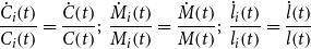 \begin{equation} \frac{\dot{C}_{i}\!\left(t\right)}{C_{i}\!\left(t\right)}=\frac{\dot{C}\!\left(t\right)}{C\!\left(t\right)};\,\,\frac{\dot{M}_{i}\!\left(t\right)}{M_{i}\!\left(t\right)}=\frac{\dot{M}\!\left(t\right)}{M\!\left(t\right)};\,\,\frac{\dot{l}_{i}\!\left(t\right)}{l_{i}\!\left(t\right)}=\frac{\dot{l}\!\left(t\right)}{l\!\left(t\right)} \end{equation}
which, in turn, implies that the aggregates grow at the same respective rates. These relationships which are a key implication of RCTD play an important role in facilitating the aggregation.
2.3. Government
Government expenditures include its spending on a publicly provided consumption good and the interest payments on its outstanding debt, while earning revenues from the taxes imposed on labor income and capital income. It finances the deficit by issuing a mixture of government bonds and nominal money. With the constraint imposed by its monetary targeting rule, it also imposes lump-sum transfers/taxes in order to ensure its intertemporal viability. Therefore, the consolidated government budget constraint expressed in real terms is
 \begin{equation} \dot{M}+\dot{B}=G+\left(R-\pi \right)\! B-\pi M-\tau \!\left[\left(r-\delta \right)\! K+wL\right]-T \end{equation}
Our focus is on the specification of monetary policy, and in particular comparing the distributional consequences of:
(i) Maintaining a constant growth rate of nominal money supply, as initially proposed by Friedman (Reference Friedman1960). For this to be sustained at the constant rate, $\overline{\theta }$
, requires that the real money growth rate is
$\overline{\theta }$
, requires that the real money growth rate is $\dot{M}(t)/M(t)=\overline{\theta }-\pi (t)$
.
$\dot{M}(t)/M(t)=\overline{\theta }-\pi (t)$
.
(ii) Pegging the nominal interest rate at $R(t)=\overline{R}$
, as initially analyzed by Poole (Reference Poole1970), with the real money supply being determined by (9c) below.
$R(t)=\overline{R}$
, as initially analyzed by Poole (Reference Poole1970), with the real money supply being determined by (9c) below.
3. Macroeconomic equilibrium
For either policy, the dynamics of the aggregate economic variables are derived by summing the optimal conditions across agents, derived in Section 2, and dividing by the population, $\mathcal{N}$
. As already noted, by employing the RCTD framework the dynamic evolution of the aggregate economic variables is determined independently of any distributional characteristics.
$\mathcal{N}$
. As already noted, by employing the RCTD framework the dynamic evolution of the aggregate economic variables is determined independently of any distributional characteristics.
3.1. Maintaining constant nominal monetary growth rate
To derive the macroeconomic equilibrium, we proceed as follows. First, summing (5b) over individual agents and using (2) we obtain $C=(1-\tau )\beta ^{-1}F_{L}(K,L)l\equiv C(K,L)=C(K,l)$
.Footnote
9
The macroeconomic equilibrium can then be described by the following dynamic equations:
$C=(1-\tau )\beta ^{-1}F_{L}(K,L)l\equiv C(K,L)=C(K,l)$
.Footnote
9
The macroeconomic equilibrium can then be described by the following dynamic equations:
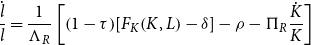
 \begin{equation} \frac{\dot{l}}{l}=\frac{1}{\Lambda _{\theta }}\left[\left(1-\tau \right)\!\left[F_{K}\!\left(K,L\right)-\delta \right]-\!\rho +\Pi _{\theta }\frac{\dot{K}}{K}+\eta \gamma \frac{\dot{M}}{M}\right] \end{equation}
 \begin{equation}\dot{K}=F(K,L)-C(K,L)-\delta K-G,\end{equation}
 \begin{equation} \frac{\dot{M}}{M}=\overline{\theta }-\eta \frac{C\!\left(K,L\right)}{M}+\left(1-\tau \right)\!\left[F_{K}\!\left(K,L\right)-\delta \right] \end{equation}
together with $L=1-l,\,\,\dot{L}=-\dot{l}$
, and where
$L=1-l,\,\,\dot{L}=-\dot{l}$
, and where $\Lambda _{\theta }\equiv \left(1-\gamma \right)\left(1+\frac{s}{\varepsilon }\frac{l}{1-l}\right)-\beta \gamma \gt 0$
,
$\Lambda _{\theta }\equiv \left(1-\gamma \right)\left(1+\frac{s}{\varepsilon }\frac{l}{1-l}\right)-\beta \gamma \gt 0$
, $\Pi _{\theta }\equiv -\left(1-\gamma \right)\frac{s}{\varepsilon }\lt 0, \mathrm{s}\equiv KF_{K}/Y$
is capital’s share of output, and
$\Pi _{\theta }\equiv -\left(1-\gamma \right)\frac{s}{\varepsilon }\lt 0, \mathrm{s}\equiv KF_{K}/Y$
is capital’s share of output, and $\varepsilon \equiv F_{K}F_{L}/FF_{KL}$
is the elasticity of substitution in production
$\varepsilon \equiv F_{K}F_{L}/FF_{KL}$
is the elasticity of substitution in production $.$
As long as the production function
$.$
As long as the production function $F(K,L)$
is a general constant returns to scale function, both
$F(K,L)$
is a general constant returns to scale function, both $s$
and
$s$
and $\boldsymbol{\varepsilon}$
are functions of the capital-labor ratio
$\boldsymbol{\varepsilon}$
are functions of the capital-labor ratio $K/L$
.Footnote
10
$K/L$
.Footnote
10
3.2. Pegging the nominal interest rate
If monetary policy takes the form of pegging the nominal interest rate at $R(t)=\overline{R}$
, the macroeconomic equilibrium is specified by:
$R(t)=\overline{R}$
, the macroeconomic equilibrium is specified by:
 \begin{equation} \frac{\dot{l}}{l}=\frac{1}{\Lambda _{R}}\left[\left(1-\tau \right)\!\left[F_{K}\!\left(K,L\right)-\delta \right]-\rho -\Pi _{R}\frac{\dot{K}}{K}\right] \end{equation}
 \begin{equation}\dot{K}=F\!\left(K,L\right)-C\!\left(K,L\right)-\delta K-G\end{equation}
where $\Lambda _{R}\equiv \!\left(1-\gamma \left(1+\eta \right)\right)\left(1+\frac{s}{\varepsilon }\frac{l}{1-l}\right)-\beta \gamma \gt 0$
,
$\Lambda _{R}\equiv \!\left(1-\gamma \left(1+\eta \right)\right)\left(1+\frac{s}{\varepsilon }\frac{l}{1-l}\right)-\beta \gamma \gt 0$
, $\Pi _{R}\equiv -\left(1-\gamma\! \left(1+\eta \right)\right)\frac{s}{\varepsilon }\lt 0$
. In this case, the real money stock is obtained by aggregating (5c), and having obtained
$\Pi _{R}\equiv -\left(1-\gamma\! \left(1+\eta \right)\right)\frac{s}{\varepsilon }\lt 0$
. In this case, the real money stock is obtained by aggregating (5c), and having obtained $K,L$
from (9a) and (9b) is determined by
$K,L$
from (9a) and (9b) is determined by
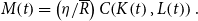 \begin{equation} M\!\left(t\right)=\left(\eta /\overline{R}\right)C\!\left(K\!\left(t\right),L\!\left(t\right)\right). \end{equation}
3.3. Steady state
Regardless of the form of monetary policy, equations (8a), (8b), (9a), and (9b) indicate that the following hold in steady state, denoted by the superscript*
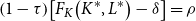 \begin{equation} \left(1-\tau \right)\!\left[F_{K}\!\left(K^{*},L^{*}\right)-\delta \right]=\rho \end{equation}
 \begin{equation} F\!\left(K^{*},L^{*}\right)-C\!\left(K^{*},L^{*}\right)-\delta K^{*}-\!G=0 \end{equation}
Therefore, the steady-state values of capital, labor (leisure), output, the wage rate, return to capital, and consumption are all determined independently of the nominal money growth rate and how it is being determined. That is, in the long run monetary policy is super-neutral insofar as these real quantities are concerned.Footnote 11
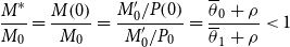
For the long-run value of inflation to be independent of how monetary policy is implemented, the steady-state values of real money balances obtained under the two monetary regimes must be equal. This will be met if the monetary authority adopts policies that satisfy $\overline{\theta }=\overline{R}-\rho$
, in which case
$\overline{\theta }=\overline{R}-\rho$
, in which case
 \begin{equation} M^{*}=\left(\eta /\!\left(\,\overline{\theta }+\rho \right)\right)C\!\left(K^{*},L^{*}\right)=\left(\eta /\overline{R}\,\right)C\!\left(K^{*},L^{*}\right). \end{equation}
Since our objective is to compare the dynamic consequences of the two forms of monetary policy, we assume that they satisfy this condition and are thus compatible with the same steady state.Footnote 12
3.4. Local aggregate dynamics
We begin by setting out the aggregate dynamics corresponding to the two forms of monetary policy.
3.4.1 Constant nominal money growth rate
To obtain the local aggregate dynamics when the monetary authority maintains the growth rate of nominal money supply constant, that is, $\theta =\overline{\theta,}$
we linearize (8) around steady state:
$\theta =\overline{\theta,}$
we linearize (8) around steady state:
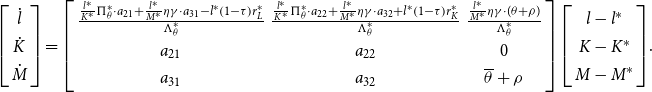 \begin{equation}\left[\begin{array}{c} \dot{l}\\ \dot{K}\\ \dot{M} \end{array}\right]=\left[\begin{array}{ccc} \frac{\frac{l^{*}}{K^{*}}\Pi _{\theta }^{*}\cdot a_{21}+\frac{l^{*}}{M^{*}}\eta \gamma \cdot a_{31}-l^{*}\left(1-\tau \right)r_{L}^{*}}{\Lambda _{\theta }^{*}} & \frac{\frac{l^{*}}{K^{*}}\Pi _{\theta }^{*}\cdot a_{22}+\frac{l^{*}}{M^{*}}\eta \gamma \cdot a_{32}+l^{*}\left(1-\tau \right)r_{K}^{*}}{\Lambda _{\theta }^{*}} & \frac{\frac{l^{*}}{M^{*}}\eta \gamma \cdot (\theta +\rho )}{\Lambda _{\theta }^{*}}\\ a_{21} & a_{22} & 0\\ a_{31} & a_{32} & \overline{\theta}+\rho \end{array}\right]\left[\begin{array}{c} l-l^{*}\\ K-K^{*}\\ M-M^{*} \end{array}\right]\!.\end{equation}
where the elements of the matrix in (11) are defined in Appendix A.1. There we suggest that under plausible conditions, convincingly met by our calibrated model, the dynamic system has one negative eigenvalue $\mu _{\theta }(\!\lt 0),$
so that all aggregate variables converge to their respective steady states at the common rate
$\mu _{\theta }(\!\lt 0),$
so that all aggregate variables converge to their respective steady states at the common rate $| \mu _{\theta }|$
.
$| \mu _{\theta }|$
.
With $l(0)$
and
$l(0)$
and $M(0)$
free to jump instantaneously in response to new information (the latter through a jump in the price level
$M(0)$
free to jump instantaneously in response to new information (the latter through a jump in the price level $P(0)$
), while
$P(0)$
), while $K(t)$
is constrained to evolve gradually from its initial value,
$K(t)$
is constrained to evolve gradually from its initial value, $K_{0}$
, the stable equilibrium paths for
$K_{0}$
, the stable equilibrium paths for $K, l$
, and
$K, l$
, and $M$
can be expressed as:
$M$
can be expressed as:
 \begin{equation} K\!\left(t\right)=K^{*}+\left(K_{0}-K^{*}\right)e^{{\mu _{\theta }}t} \end{equation}
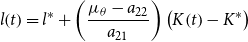 \begin{equation} l\!\left(t\right)=l^{*}+\left(\frac{\mu _{\theta }-a_{22}}{a_{21}}\right)\left(K\!\left(t\right)-K^{*}\right) \end{equation}
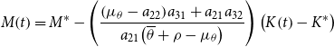 \begin{equation} M\!\left(t\right)=M^{*}-\left(\frac{\left(\mu _{\theta }-a_{22}\right)\! a_{31}+a_{21}a_{32}}{a_{21}\!\left(\overline{\theta }+\rho -\mu _{\theta }\right)}\right)\left(K\!\left(t\right)-K^{*}\right) \end{equation}
In Appendix A.1, it is noted that while sgn ( $\mu _{\theta }-a_{22}$
) is potentially ambiguous, it is most likely negative, as is certainly the case in our simulations. In that case, if the economy experiences an expansion in the aggregate capital stock
$\mu _{\theta }-a_{22}$
) is potentially ambiguous, it is most likely negative, as is certainly the case in our simulations. In that case, if the economy experiences an expansion in the aggregate capital stock $(K_{0}\lt K^{*})$
, following initial jumps, average leisure,
$(K_{0}\lt K^{*})$
, following initial jumps, average leisure, $l(t)$
, and real balances,
$l(t)$
, and real balances, $M(t)$
, will both increase monotonically to their respective steady-state values,
$M(t)$
, will both increase monotonically to their respective steady-state values, $l^{*}$
and
$l^{*}$
and $M^{*}$
, during the subsequent transition.Footnote
13
$M^{*}$
, during the subsequent transition.Footnote
13
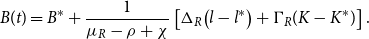
Using the government budget constraint, (7), and the transversality condition, (5f), the time path for government bonds, $B(t),$
can be solved in the neighborhood of the steady state as:
$B(t),$
can be solved in the neighborhood of the steady state as:
 \begin{equation}B\!\left(t\right)=B^{*}+\frac{1}{\mu _{\theta }-\rho +\chi }\left[\Delta _{\theta }\!\left(l\!\left(t\right)-l^{*}\right)+\Gamma _{\theta }\!\left(K\!\left(t\right)-K^{*}\right)-\left(\theta +\chi \right)\left(M\!\left(t\right)-M^{*}\right)\right],\end{equation}
where $\Delta _{\theta }$
and
$\Delta _{\theta }$
and $\Gamma _{\theta }$
are defined in Appendix A.1, and the derivation of (13) is also provided. There we point out that to satisfy the transversality condition, and with the nominal stock of bonds being sluggish,
$\Gamma _{\theta }$
are defined in Appendix A.1, and the derivation of (13) is also provided. There we point out that to satisfy the transversality condition, and with the nominal stock of bonds being sluggish, $B^{*}$
and
$B^{*}$
and $\chi$
are set so as to satisfy the appropriate initial and steady-state conditions for (13), given by (A5a) and (A5b). In equilibrium, government bonds also converge at the rate
$\chi$
are set so as to satisfy the appropriate initial and steady-state conditions for (13), given by (A5a) and (A5b). In equilibrium, government bonds also converge at the rate $| \mu _{\theta }| .$
3.4.2 Pegging the nominal interest rate
If monetary policy is specified in terms of pegging the nominal interest rate, that is, $R(t)=\overline{R}$
, the local transitional dynamics are described by:
$R(t)=\overline{R}$
, the local transitional dynamics are described by:
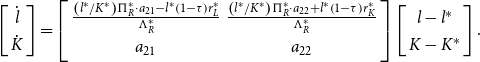 \begin{equation}\left[\begin{array}{c} \dot{l}\\ \dot{K} \end{array}\right]=\left[\begin{array}{cc} \frac{\left(l^{*}/K^{*}\right)\Pi _{R}^{*}\cdot a_{21}-l^{*}\left(1-\tau \right)r_{L}^{*}}{\Lambda _{R}^{*}} & \frac{\left(l^{*}/K^{*}\right)\Pi _{R}^{*}\cdot a_{22}+l^{*}\left(1-\tau \right)r_{K}^{*}}{\Lambda _{R}^{*}}\\ a_{21} & a_{22} \end{array}\right]\left[\begin{array}{c} l-l^{*}\\ K-K^{*} \end{array}\right].\end{equation}
where the elements of the matrix are defined in Appendix A.2. In this case, one of the two eigenvalues is negative, $\mu _{R}(\!\lt 0),$
so that all aggregate variables converge to their steady state at the common rate
$\mu _{R}(\!\lt 0),$
so that all aggregate variables converge to their steady state at the common rate $| \mu _{R}| .$
From (14), the saddle path describing the transitional dynamics of capital and leisure is described by (12a) and (12b), with
$| \mu _{R}| .$
From (14), the saddle path describing the transitional dynamics of capital and leisure is described by (12a) and (12b), with $\mu _{R}$
replacing
$\mu _{R}$
replacing $\mu _{\theta }$
. The transitional path of real money supply tracks that of consumption in accordance with equation (9c), while the dynamics of government bonds are now
$\mu _{\theta }$
. The transitional path of real money supply tracks that of consumption in accordance with equation (9c), while the dynamics of government bonds are now
 \begin{equation}B(t)=B^{*}+\frac{1}{\mu _{R}-\rho +\chi }\left[\Delta _{R}\!\left(l-l^{*}\right)+\Gamma _{R}(K-K^{*})\right].\end{equation}
subject to the constraints (A8a) and (A8b), and where $\Delta _{R}$
and
$\Delta _{R}$
and $\Gamma _{R}$
are defined in Appendix A.2.
$\Gamma _{R}$
are defined in Appendix A.2.
These results depend in part upon the form of the underlying utility function (3) and may be summarized by the following observations:
-
(i) The steady states of the real variables (output, employment, capital, consumption) are independent of how monetary policy is conducted.
-
(ii) The steady state of the monetary variables (inflation and real money) is independent of how monetary policy is conducted, provided $\overline{\theta }=\overline{R}-\rho$
.
$\overline{\theta }=\overline{R}-\rho$
. -
(iii) The differential effects of targeting the monetary growth rate or pegging the nominal interest rate on the transitional paths of the real variables operate entirely through its impact on their respective adjustment speeds,
$| \mu _{\theta }|$
,
$| \mu _{R}|$
. -
(iv) The differential effects on transitional paths of the monetary variables reflect both the differential adjustment speeds,
$| \mu _{\theta }| | \mu _{R}|,$
and the initial jump in the price level necessary for the real money supply to follow the respective stable transitional paths (12c), (9c).


4. Dynamics of wealth and income inequality
We now turn to the implications for the distributions of wealth and income. Since the impact of monetary policy manifests itself through the aggregate variables discussed in the previous section, no further identification of the specific form of monetary policy is necessary. Also, because this procedure is adapted from our earlier work, details are relegated to Appendix B. Instead, our focus here is to identify the various channels whereby aggregate variables influence the distribution.
4.1. Relative wealth and wealth inequality
The evolution of the relative wealth of individual i, described by equations (B3) and (B4), reflects two underlying sources of dynamics. First are those of the aggregate variables, $K(t),\,\,l(t)$
, described by (11) and (14), that generate the returns to capital and labor for the two forms of monetary policy. Second are the internal dynamics of relative wealth,
$K(t),\,\,l(t)$
, described by (11) and (14), that generate the returns to capital and labor for the two forms of monetary policy. Second are the internal dynamics of relative wealth, $a_{i}(t)$
, which depend upon the coefficient of
$a_{i}(t)$
, which depend upon the coefficient of $a_{i}$
in (B1) evaluated at steady state, and under weak restrictions can be shown to be positive. Specifically, if private consumption exceeds after-tax labor income, then aggregating the optimality condition, (5b), over individuals implies
$a_{i}$
in (B1) evaluated at steady state, and under weak restrictions can be shown to be positive. Specifically, if private consumption exceeds after-tax labor income, then aggregating the optimality condition, (5b), over individuals implies $l^{*}\gt \beta /(1+\beta )$
which in turn ensuresFootnote
14
$l^{*}\gt \beta /(1+\beta )$
which in turn ensuresFootnote
14
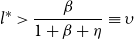 \begin{equation} l^{*}\gt \frac{\beta }{1+\beta +\eta }\equiv \upsilon \end{equation}
Imposing (16), (B2) then implies that the greater is an agent’s steady-state relative wealth, the more leisure he enjoys and the less labor he supplies. This reflects the fact that wealthier agents have a lower marginal utility of wealth.Footnote 15
In general, the individual’s initial relative wealth, $a_{i}(0)$
, is endogenous. This is because money and bonds, being denominated in nominal terms, are subject to real shocks due to the jump in the price level,
$a_{i}(0)$
, is endogenous. This is because money and bonds, being denominated in nominal terms, are subject to real shocks due to the jump in the price level, $P(0)$
, at the time a policy change or structural change occurs. Equation (C2) sets out the relationship between the jump in
$P(0)$
, at the time a policy change or structural change occurs. Equation (C2) sets out the relationship between the jump in $P(0)$
and initial relative wealth, showing that the impact of
$P(0)$
and initial relative wealth, showing that the impact of $P(0)$
on
$P(0)$
on $a_{i}(0)$
depends upon the difference between the individual’s allocation between the real asset (capital) and the nominal assets (money plus bonds,
$a_{i}(0)$
depends upon the difference between the individual’s allocation between the real asset (capital) and the nominal assets (money plus bonds, $N_{0}$
) and the economy-wide allocation.
$N_{0}$
) and the economy-wide allocation.
Because of the linearity of (C3) and (C4), we can readily transform these equations into a relationship describing the evolution of the standard deviation of wealth across agents, $\sigma _{a}(t)$
, which serves as a convenient and tractable summary measure of wealth inequality:
$\sigma _{a}(t)$
, which serves as a convenient and tractable summary measure of wealth inequality:
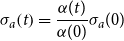 \begin{equation}\sigma _{a}\!\left(t\right)=\frac{\alpha (t)}{\alpha (0)}\sigma _{a}(0)\end{equation}
and which converges in steady state to $\sigma _{a}^{*}=\frac{1}{\alpha (0)}\cdot \sigma _{a}(0)$
. Equation (17) highlights how the evolution of
$\sigma _{a}^{*}=\frac{1}{\alpha (0)}\cdot \sigma _{a}(0)$
. Equation (17) highlights how the evolution of $\sigma _{a}(t)$
is driven by two factors, (i) initial wealth inequality,
$\sigma _{a}(t)$
is driven by two factors, (i) initial wealth inequality, $\sigma _{a}(0)$
, and (ii) the evolution of relative wealth,
$\sigma _{a}(0)$
, and (ii) the evolution of relative wealth, $a_{i}(t)$
, driven by
$a_{i}(t)$
, driven by $\alpha (t)$
, defined in (B3).
$\alpha (t)$
, defined in (B3).
Appendix C shows that the initial post-shock wealth inequality across individuals is
 \begin{equation} \sigma _{a}\!\left(0\right)=\left[\left(1-\varpi \right)^{2}\sigma _{k,0}^{2}+2\!\left(1-\varpi \right)\varpi \sigma _{k,0}\sigma _{n,0}\nu +\varpi ^{2}\sigma _{n,0}^{2}\right]^{1/2} \end{equation}
where $\varpi \equiv N_{0}/(P(0)K_{0}+N_{0})$
is the ratio of nominal assets to total wealth,
$\varpi \equiv N_{0}/(P(0)K_{0}+N_{0})$
is the ratio of nominal assets to total wealth, $\sigma _{k,0},\sigma _{n,0}$
are standard deviations of the initial endowments, and
$\sigma _{k,0},\sigma _{n,0}$
are standard deviations of the initial endowments, and $\nu$
is the correlation of endowments across agents. It is evident from (18) that one channel through which any shock impinges on wealth inequality is via its impact on the initial price level,
$\nu$
is the correlation of endowments across agents. It is evident from (18) that one channel through which any shock impinges on wealth inequality is via its impact on the initial price level, $P(0)$
, and how this interacts with the pattern of initial endowments and their distribution, see equation (C5). There we show that if: (i) the economy-wide endowment of capital exceeds that of financial assets (
$P(0)$
, and how this interacts with the pattern of initial endowments and their distribution, see equation (C5). There we show that if: (i) the economy-wide endowment of capital exceeds that of financial assets ( $\varpi \lt 1/2$
), and (ii) nominal assets are less unequally endowed across agents than is capital (
$\varpi \lt 1/2$
), and (ii) nominal assets are less unequally endowed across agents than is capital ( $\sigma _{n,0}\leq \sigma _{k,0}$
), an increase in the initial price level will increase initial wealth inequality. This is because an increase in
$\sigma _{n,0}\leq \sigma _{k,0}$
), an increase in the initial price level will increase initial wealth inequality. This is because an increase in $P(0)$
will increase the relative quantity of capital in agents’ portfolios, and since wealthier agents hold relatively more capital, wealth inequality will increase; the opposite applies to a decrease in
$P(0)$
will increase the relative quantity of capital in agents’ portfolios, and since wealthier agents hold relatively more capital, wealth inequality will increase; the opposite applies to a decrease in $P(0)$
. We view the conditions (i) and (ii) as entirely plausible and shall refer to this channel as “the initial price response” channel.
$P(0)$
. We view the conditions (i) and (ii) as entirely plausible and shall refer to this channel as “the initial price response” channel.
This impact on initial wealth inequality persists throughout the subsequent evolution of wealth inequality, as implied by (17). But during the transition, the other channel, $\alpha (t)$
, defined by (B3), comes into effect. From (B3) we see that
$\alpha (t)$
, defined by (B3), comes into effect. From (B3) we see that $\alpha (t)$
declines as leisure increases over time. This is because the positive relationship between leisure and capital described by the aggregate dynamics, (12b) and (14), implies that if capital is accumulated over time, labor supply falls, causing the capital-labor ratio to increase. This in turn implies that during the transition an increasing wage rate is accompanied by a declining return to capital, which favors the less affluent, leading to a steady decline in wealth inequality over time. This effect, which reflects the changing productivity of capital and labor, can be termed the “wage-return to capital” channel.
$\alpha (t)$
declines as leisure increases over time. This is because the positive relationship between leisure and capital described by the aggregate dynamics, (12b) and (14), implies that if capital is accumulated over time, labor supply falls, causing the capital-labor ratio to increase. This in turn implies that during the transition an increasing wage rate is accompanied by a declining return to capital, which favors the less affluent, leading to a steady decline in wealth inequality over time. This effect, which reflects the changing productivity of capital and labor, can be termed the “wage-return to capital” channel.
4.2. Relative income and income inequality
From equation (B8a), we see that relative income is driven in part by relative wealth. To describe this channel, we need to determine the agent’s position in real money balances, M, and income-yielding assets, $V\equiv K+B$
, relative to his overall wealth. These are given by equations (B5) and (B6), respectively. In the case of the latter, with capital and bonds yielding the same rate of return, and in the absence of risk, investors view these two assets as perfect substitutes, enabling us to characterize only their composite distribution (
$V\equiv K+B$
, relative to his overall wealth. These are given by equations (B5) and (B6), respectively. In the case of the latter, with capital and bonds yielding the same rate of return, and in the absence of risk, investors view these two assets as perfect substitutes, enabling us to characterize only their composite distribution ( $v_{i}\equiv V_{i}/V$
). Comparing (B5) and (B6), we see that the relative asset holdings of an agent who has above average wealth,
$v_{i}\equiv V_{i}/V$
). Comparing (B5) and (B6), we see that the relative asset holdings of an agent who has above average wealth, $a_{i}(t)\gt 1$
are:
$a_{i}(t)\gt 1$
are: $v_{i}(t)-1\gt a_{i}(t)-1\gt M_{i}/M-1,$
meaning that his portfolio comprises disproportionately more of the income-earning assets, and less money than his overall relative wealth position represents. For a relatively poor agent,
$v_{i}(t)-1\gt a_{i}(t)-1\gt M_{i}/M-1,$
meaning that his portfolio comprises disproportionately more of the income-earning assets, and less money than his overall relative wealth position represents. For a relatively poor agent, $a_{i}(t)\lt 1$
, the opposite applies.
$a_{i}(t)\lt 1$
, the opposite applies.
Of the several potential measures of income inequality, we shall focus on before-tax personal income, defined as income from the income-earning assets, (capital and bonds) plus income from labor. Thus, the relative before-tax personal income of agent i is $y_{i}(t)\equiv Y_{i}(t)/Y(t)=[r(t)V_{i}(t)+w(t)L_{i}(t)][r(t)V(t)+w(t)L(t)]^{-1}$
, which is related to the agent’s relative wealth by (B8a) and (B8b). This can then be transformed to the following relationship between income inequality and wealth inequality:
$y_{i}(t)\equiv Y_{i}(t)/Y(t)=[r(t)V_{i}(t)+w(t)L_{i}(t)][r(t)V(t)+w(t)L(t)]^{-1}$
, which is related to the agent’s relative wealth by (B8a) and (B8b). This can then be transformed to the following relationship between income inequality and wealth inequality:
 \begin{equation} \sigma _{y}\!\left(t\right)=\varphi\! \left(t\right)\sigma _{a}\!\left(t\right) \end{equation}
where
 \begin{equation} \varphi\! \left(t\right)\equiv \frac{1}{Y\!\left(t\right)+r\!\left(t\right)B\!\left(t\right)}\left\{r\!\left(t\right)A\!\left(t\right)-\left(r\!\left(t\right)M\!\left(t\right)+w\!\left(t\right)l\!\left(t\right)\right)\left(1-\frac{\upsilon }{l^{*}}\right)\frac{1}{\alpha\! \left(t\right)}\right\} \end{equation}
The term $\varphi (t)$
measures the income generated by the individual’s portfolio of assets, as reflected in his relative wealth. Because of the homogeneity of the underlying utility function, it is driven by economy-wide averages and is therefore common to all individuals. It comprises two components: (i) the share of personal income from the income-earning assets, bonds plus capital, and (ii) relative labor income, reflected in the second term, which reflects the fact that more (less) wealthy agents supply less (more) labor. In our benchmark calibration, the second term, which is negative, is dominated by the first term, implying
$\varphi (t)$
measures the income generated by the individual’s portfolio of assets, as reflected in his relative wealth. Because of the homogeneity of the underlying utility function, it is driven by economy-wide averages and is therefore common to all individuals. It comprises two components: (i) the share of personal income from the income-earning assets, bonds plus capital, and (ii) relative labor income, reflected in the second term, which reflects the fact that more (less) wealthy agents supply less (more) labor. In our benchmark calibration, the second term, which is negative, is dominated by the first term, implying $0\lt \varphi (t)\lt 1$
. In steady state, (19) converges to:
$0\lt \varphi (t)\lt 1$
. In steady state, (19) converges to:
 \begin{equation} \sigma _{y}^{*}=\varphi ^{*}\sigma _{a}^{*}=\left[r^{*}A^{*}-\left(r^{*}M^{*}+w^{*}l^{*}\right)\!\left(1-\upsilon /l^{*}\right)\right]\!\left[Y^{*}+r^{*}B^{*}\right]^{-1}\sigma _{a}^{*} \end{equation}
We conclude with two observations. First, it is apparent from (20) that the two channels through which the aggregate variables impinge on wealth inequality, $\sigma _{a}(t)$
, also indirectly impact income inequality. But by influencing
$\sigma _{a}(t)$
, also indirectly impact income inequality. But by influencing $\varphi (t)$
, they will exert an additional direct impact on income inequality. In the short run, the discrete change in the price level,
$\varphi (t)$
, they will exert an additional direct impact on income inequality. In the short run, the discrete change in the price level, $P(0)$
, will impact the real income generated by government bonds, which in addition to any initial jumps in
$P(0)$
, will impact the real income generated by government bonds, which in addition to any initial jumps in $l(0)$
and its impact on
$l(0)$
and its impact on $r(0)$
and
$r(0)$
and $w(0)$
will impact
$w(0)$
will impact $\varphi (0)$
. Over time,
$\varphi (0)$
. Over time, $\varphi (t)$
will continue to reflect the evolving returns to capital and wage rate embodied in the wage-return to capital channel. Second, the effects of the channels we have identified are highly sensitive to the source of the structural change and specifically whether they reflect demand or supply shocks. As we demonstrate below, both analytically and in our simulations, this is because they lead to opposite responses in
$\varphi (t)$
will continue to reflect the evolving returns to capital and wage rate embodied in the wage-return to capital channel. Second, the effects of the channels we have identified are highly sensitive to the source of the structural change and specifically whether they reflect demand or supply shocks. As we demonstrate below, both analytically and in our simulations, this is because they lead to opposite responses in $P(0)$
, which have opposite effects on the initial wealth inequality, which then persist over time.
$P(0)$
, which have opposite effects on the initial wealth inequality, which then persist over time.
5. Nominal monetary expansion and inequality
In this section, we compare the impacts of monetary expansions under the two modes of monetary policy—setting $\theta =\overline{\theta }$
and pegging
$\theta =\overline{\theta }$
and pegging $R=\overline{R}$
—on inequality. In both cases, the economy starts out from the same initial steady state,
$R=\overline{R}$
—on inequality. In both cases, the economy starts out from the same initial steady state, $\overline{\theta }_{0}=\overline{R}_{0}-\rho$
, the only difference being in the form of the nominal monetary expansion. In the first case, it occurs via an increase in the money growth from
$\overline{\theta }_{0}=\overline{R}_{0}-\rho$
, the only difference being in the form of the nominal monetary expansion. In the first case, it occurs via an increase in the money growth from $\overline{\theta }_{0}$
to
$\overline{\theta }_{0}$
to $\overline{\theta }_{1}$
; in the latter case, it is accomplished by a reduction in the nominal interest rate from
$\overline{\theta }_{1}$
; in the latter case, it is accomplished by a reduction in the nominal interest rate from $\overline{R}_{0}$
to
$\overline{R}_{0}$
to $\overline{R}_{1}$
. In either case, the real capital stock remains unchanged at its initial level,
$\overline{R}_{1}$
. In either case, the real capital stock remains unchanged at its initial level, $K_{0}$
, implying that
$K_{0}$
, implying that $l,\,\,L,\,\,Y,C$
also remain unchanged at their initial equilibrium levels.Footnote
16
$l,\,\,L,\,\,Y,C$
also remain unchanged at their initial equilibrium levels.Footnote
16
There are no transitional dynamics. The required adjustment is that the real stock of money must jump instantaneously in order for the equilibrium marginal rate of substitution between money and consumption, (10c), to be maintained. If the nominal money supply and government debt are constrained to evolve gradually, the required equilibrating adjustment occurs through a jump in the price level.Footnote 17
Recalling (10c), increasing the money growth rate from $\overline{\theta }_{0}$
to
$\overline{\theta }_{0}$
to $\overline{\theta }_{1}$
implies an immediate reduction in real money balances, attained by an increase in price from its pre-shock level,
$\overline{\theta }_{1}$
implies an immediate reduction in real money balances, attained by an increase in price from its pre-shock level, $P_{0}$
. Let
$P_{0}$
. Let $M_{0},M^{\prime}_{0}$
denote the pre-shock levels of the real and nominal money stocks:
$M_{0},M^{\prime}_{0}$
denote the pre-shock levels of the real and nominal money stocks:
 \begin{equation} \frac{M^{*}}{M_{0}}=\frac{M\!\left(0\right)}{M_{0}}=\frac{M^{\prime}_{0}/P\!\left(0\right)}{M^{\prime}_{0}/P_{0}}=\frac{\overline{\theta }_{0}+\rho }{\overline{\theta }_{1}+\rho }\lt 1 \end{equation}
which implies
 \begin{equation} \frac{dB\!\left(0\right)}{B\!\left(0\right)}=\frac{dM\!\left(0\right)}{M\!\left(0\right)}=\frac{P_{0}-P\!\left(0\right)}{P_{0}}=-\frac{dP\!\left(0\right)}{P_{0}}=\frac{\overline{\theta }_{0}-\overline{\theta }_{1}}{\overline{\theta }_{0}+\rho }\lt 0 \end{equation}
where the proportionate change in bonds follows from the government budget constraint, (A5a).
With $l(t)$
unchanged at its initial steady state, (B3) implies
$l(t)$
unchanged at its initial steady state, (B3) implies $\alpha (t)=\alpha (0)=1$
, and (17) implies
$\alpha (t)=\alpha (0)=1$
, and (17) implies $\sigma _{a}^{*}=\sigma _{a}(t)=\sigma _{a}(0)$
, where recalling (18),
$\sigma _{a}^{*}=\sigma _{a}(t)=\sigma _{a}(0)$
, where recalling (18), $\sigma _{a}(0)$
is endogenously determined due to the initial jump in the price level reported in (21’). As shown in equation (C5), the effect of the price jump on
$\sigma _{a}(0)$
is endogenously determined due to the initial jump in the price level reported in (21’). As shown in equation (C5), the effect of the price jump on $\sigma _{a}(0)$
depends critically upon: the relative importance of nominal assets in economy-wide wealth (
$\sigma _{a}(0)$
depends critically upon: the relative importance of nominal assets in economy-wide wealth ( $\varpi$
), and the relative variations in the initial endowments of financial versus real assets across individuals (
$\varpi$
), and the relative variations in the initial endowments of financial versus real assets across individuals ( $\sigma _{n,0}/\sigma _{k,0}$
). Under the previously identified weak conditions (
$\sigma _{n,0}/\sigma _{k,0}$
). Under the previously identified weak conditions ( $\varpi \lt 1/2, \sigma _{n,0}\leq \sigma _{k,0}$
), (C5) implies
$\varpi \lt 1/2, \sigma _{n,0}\leq \sigma _{k,0}$
), (C5) implies $d\sigma _{a}^{*}/dP(0)=d\sigma _{a}(0)/dP(0)\gt 0$
.
$d\sigma _{a}^{*}/dP(0)=d\sigma _{a}(0)/dP(0)\gt 0$
.
Under these same conditions, a monetary expansion brought about by a reduction in the nominal interest rate yields
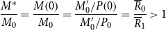 \begin{equation} \frac{M^{*}}{M_{0}}=\frac{M\!\left(0\right)}{M_{0}}=\frac{M^{\prime}_{0}/P\!\left(0\right)}{M^{\prime}_{0}/P_{0}}=\frac{\overline{R}_{0}}{\overline{R}_{1}}\gt 1 \end{equation}
which implies
 \begin{equation} \frac{dB\!\left(0\right)}{B\!\left(0\right)}=\frac{dM\!\left(0\right)}{M\!\left(0\right)}=\frac{P_{0}-P\!\left(0\right)}{P_{0}}=-\frac{dP\!\left(0\right)}{P_{0}}=\frac{\overline{R}_{0}-\overline{R}_{1}}{\overline{R}_{0}}\gt 0 \end{equation}
In this case, the reduction in the nominal interest rate reduces the initial price level, in which case under the conditions ( $\varpi \lt 1/2,\sigma _{n,0}\leq \sigma _{k,0}$
) we obtain
$\varpi \lt 1/2,\sigma _{n,0}\leq \sigma _{k,0}$
) we obtain $d\sigma _{a}^{*}/dP(0)=d\sigma _{a}(0)/dP(0)\lt 0$
.
$d\sigma _{a}^{*}/dP(0)=d\sigma _{a}(0)/dP(0)\lt 0$
.
Turning now to income inequality, again there are no transitional dynamics. Given the response in wealth inequality, the effect on income inequality is
 \begin{equation} d\sigma _{y}^{*}/\sigma _{y}^{*}=d\varphi ^{*}/\varphi ^{*}+d\sigma _{a}^{*}/\sigma _{a}^{*} \end{equation}
where
 \begin{equation} \frac{d\varphi ^{*}}{dP\!\left(0\right)/P_{0}}=-\frac{r^{*}}{\left(Y^{*}+r^{*}B^{*}\right)^{2}}\left[\left(M^{*}\upsilon Y^{*}/l^{*}\right)+w^{*}\left(1-\upsilon \right)B^{*}\right]\lt 0 \end{equation}
implying that an increase (decrease) in the initial price level reduces (raises) the real income generating effect of wealth, $\varphi ^{*}$
. The impact on income inequality reflects two effects. First, to the extent that the price rise increases wealth inequality it also directly increases income inequality. But, in addition, the discrete price increase reduces the real value of government bonds, and therefore the interest income they generate. Since these bonds are held more proportionately by wealthier agents, this reduces the degree of income inequality. The net impact on income inequality thus depends upon the relative sizes of these two offsetting effects. Comparing (23) and (C5), we see that the two effects are essentially determined independently. Accordingly, income inequality may quite plausibly rise or fall with increasing wealth inequality.
$\varphi ^{*}$
. The impact on income inequality reflects two effects. First, to the extent that the price rise increases wealth inequality it also directly increases income inequality. But, in addition, the discrete price increase reduces the real value of government bonds, and therefore the interest income they generate. Since these bonds are held more proportionately by wealthier agents, this reduces the degree of income inequality. The net impact on income inequality thus depends upon the relative sizes of these two offsetting effects. Comparing (23) and (C5), we see that the two effects are essentially determined independently. Accordingly, income inequality may quite plausibly rise or fall with increasing wealth inequality.
The notable feature is that the two forms of monetary expansion have precisely the opposite impacts on wealth and income inequality and can be summarized in the following proposition, specified for the more plausible case where $d\sigma _{a}^{*}/dP(0)=d\sigma _{a}(0)/dP(0)\gt 0$
.
$d\sigma _{a}^{*}/dP(0)=d\sigma _{a}(0)/dP(0)\gt 0$
.
Proposition 1:
-
(i) A nominal monetary expansion specified by an increase in the monetary growth rate increases the price level, reducing the value of the nominal assets and causing wealth inequality to increase. This is offset by a decline in the income generating effect of wealth,
$\varphi ^{*}$
, with the net impact on income inequality depending upon which effect dominates. -
(ii) If the monetary expansion takes the form of a reduction in the nominal interest rate, precisely the opposite occurs. The price level falls, wealth inequality declines, and
$\varphi ^{*}$
increases, with the net impact on income inequality depending upon which effect dominates.


Any apparent contradiction between these two forms of nominal monetary expansion is readily resolved by observing that with perfectly flexible prices the initial jump in the price level following an increase in the nominal monetary growth rate dominates the (gradually) growing nominal money supply. The real stock of money immediately declines, so paradoxically, this turns out to be a contractionary policy in real terms. In contrast, reducing the nominal interest rate directly stimulates the real demand for money and is expansionary.
An interesting aspect of Proposition 1 is that although neither form of monetary expansion affects the economy’s real productive capacity—both leaving $K,L,Y,C$
unchanged at their initial levels—the difference is that (i) increases the inflation rate, while (ii) reduces it. In view of the fact that much of the empirical literature view the monetary policy–inequality relationship in terms of inflation, it is useful to re-express the proposition in these terms.Footnote
18
$K,L,Y,C$
unchanged at their initial levels—the difference is that (i) increases the inflation rate, while (ii) reduces it. In view of the fact that much of the empirical literature view the monetary policy–inequality relationship in terms of inflation, it is useful to re-express the proposition in these terms.Footnote
18
Proposition 2: Monetary policy that increases the rate of inflation will increase wealth inequality. Its effect on income inequality depends upon whether the increase in wealth inequality dominates its effect on the income generating effect of wealth, $\varphi ^{*}$
.
$\varphi ^{*}$
.
Table 1 provides some numerical examples illustrating the ranges of likely responses of wealth and income inequality due to the price change associated with the monetary expansion. The parameters are based on the calibration discussed in Section 6, below. In the absence of any solid information on the relative magnitudes of the distribution of initial endowments, $\sigma _{n,0}/\sigma _{k,0}\equiv \lambda$
, and their correlation,
$\sigma _{n,0}/\sigma _{k,0}\equiv \lambda$
, and their correlation, $\nu$
, we let these two parameters vary over the range indicated in the table. In all cases, increasing the monetary growth rate by 1 percentage point (p.p.) increases wealth inequality, while decreasing the nominal interest rate by 1 p.p. reduces wealth inequality. As is readily seen, the comparative impacts on wealth and income inequality are sensitive to both
$\nu$
, we let these two parameters vary over the range indicated in the table. In all cases, increasing the monetary growth rate by 1 percentage point (p.p.) increases wealth inequality, while decreasing the nominal interest rate by 1 p.p. reduces wealth inequality. As is readily seen, the comparative impacts on wealth and income inequality are sensitive to both $\lambda$
and
$\lambda$
and $\nu$
. The examples suggest that if
$\nu$
. The examples suggest that if $\nu \geq 0$
, the income generating effect dominates so that wealth and income inequality are impacted in opposite ways, But if nominal and real assets are negatively correlated, the wealth effect dominates and wealth and income inequality respond in the same direction. In light of (B5) and (B6), which imply that poor agents hold relatively more money than do affluent agents, the negatively correlated case
$\nu \geq 0$
, the income generating effect dominates so that wealth and income inequality are impacted in opposite ways, But if nominal and real assets are negatively correlated, the wealth effect dominates and wealth and income inequality respond in the same direction. In light of (B5) and (B6), which imply that poor agents hold relatively more money than do affluent agents, the negatively correlated case $\nu \lt 0$
seems plausible.Footnote
19
$\nu \lt 0$
seems plausible.Footnote
19
Changes in inequality in response to changes in monetary policy
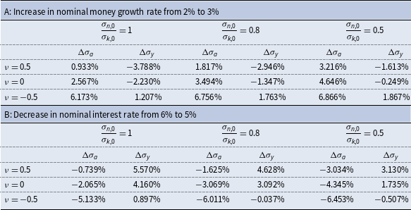
NB Table 1A also obtains for (i) increase in nominal interest rate from 6% to 7%; (ii) increase in inflation target from 2% to 3%. Table 1B also obtains for (i) decrease in nominal money growth rate from 2% to 1%; (ii) decrease in inflation target from 2% to 1%. $\sigma _{k,0},\sigma _{n,0}$
denote initial distributions of capital and nominal assets across agents.
$\sigma _{k,0},\sigma _{n,0}$
denote initial distributions of capital and nominal assets across agents. $\nu$
denotes correlation between initial distributions of capital and nominal assets across agents.
$\nu$
denotes correlation between initial distributions of capital and nominal assets across agents.
6. Calibration
While monetary policy in isolation does not generate transitional dynamics, it does influence the transitional path generated by real structural changes, such as an increase in technology. To compare the dynamic responses of the economy to such changes under the alternative monetary policies, we employ numerical simulations.
The parameter values we adopt for this purpose are reported in Table 2 and are chosen to be consistent with US parameters over the last decade, insofar as is feasible for a small stylized model such as this. In choosing these values, we should also note the following. In the case of the aggregate economy-wide average variables, we assume that the monetary policies are consistent with a common steady state. However, this does not yield the same rate of convergence among the different monetary policies, although the differences are small. This is important since the nature of the transition, and in particular the speed of convergence, is a critical determinant of the responses in the various inequality measures to the alternative shocks. A characteristic of the RCTD approach to distribution being adopted is that all measures of inequality are relative to those of initial wealth, which is arbitrarily given and normalized to unity. In the initial equilibrium, the steady-state values of the standard deviations of wealth, income-earning assets, and income are identical among the three monetary policies.
Basic parameters (benchmark)
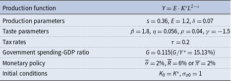
The production function is Cobb-Douglas, with the capital elasticity being set at its conventional value, $s=0.36$
, TFP is
$s=0.36$
, TFP is $E=$
1.2, while the annual rate of depreciation is assumed to be 7%. This yields an equilibrium capital-output ratio of 3.
$E=$
1.2, while the annual rate of depreciation is assumed to be 7%. This yields an equilibrium capital-output ratio of 3.
Regarding the parameters pertaining to utility, the rate of time preference, $\rho =0.04$
, is standard, while the IES corresponding to
$\rho =0.04$
, is standard, while the IES corresponding to $\gamma =-1.5(0.4)$
is well within the estimated range as reported by Guvenen (Reference Guvenen2006) and Havranek et al. (Reference Havranek, Horvath, Irsova and Rusnak2015). The elasticity of leisure in utility is the critical factor determining the agent’s allocation of time, and setting
$\gamma =-1.5(0.4)$
is well within the estimated range as reported by Guvenen (Reference Guvenen2006) and Havranek et al. (Reference Havranek, Horvath, Irsova and Rusnak2015). The elasticity of leisure in utility is the critical factor determining the agent’s allocation of time, and setting $\beta =1.8$
yields the steady-state allocation of time to leisure of
$\beta =1.8$
yields the steady-state allocation of time to leisure of $l^{*}=0.6919$
which is comparable to the evidence provided by Cooley (Reference Cooley1995) and other related studies.
$l^{*}=0.6919$
which is comparable to the evidence provided by Cooley (Reference Cooley1995) and other related studies.
Information on $\eta$
is less direct. In the case of real money balances, our choice of
$\eta$
is less direct. In the case of real money balances, our choice of $\eta =0.056$
is justified as follows. First, it depends upon how broadly one views money with respect to the utility benefits it provides. For this purpose we adopt the broad measure, M3. The implied value of the real money balances becomes
$\eta =0.056$
is justified as follows. First, it depends upon how broadly one views money with respect to the utility benefits it provides. For this purpose we adopt the broad measure, M3. The implied value of the real money balances becomes $M^{*}=0.4531$
, so that the real money balance to consumption ratio is
$M^{*}=0.4531$
, so that the real money balance to consumption ratio is $M^{*}/C^{*}=0.9333.$
The average value of the real M3-consumption ratio for the period 2002–2020 in the USA is 0.88, suggesting that the parameter choices pertaining to money are generally consistent with the data.
$M^{*}/C^{*}=0.9333.$
The average value of the real M3-consumption ratio for the period 2002–2020 in the USA is 0.88, suggesting that the parameter choices pertaining to money are generally consistent with the data.
With regard to monetary policy, many advanced economies set a target rate of inflation equal to 2%. Accordingly, we set the growth rate of nominal money supply at $\overline{\theta }=$
2%, nominal interest rate at
$\overline{\theta }=$
2%, nominal interest rate at $\overline{R}=6\mathrm{\% }$
so that the steady-state inflation rate becomes 2% for both monetary policies.Footnote
20
With the inflation rate in the USA from 2000 to 2020 averaging around 1.70%, this value is also compatible with US experience.
$\overline{R}=6\mathrm{\% }$
so that the steady-state inflation rate becomes 2% for both monetary policies.Footnote
20
With the inflation rate in the USA from 2000 to 2020 averaging around 1.70%, this value is also compatible with US experience.
For fiscal policies, the average value of the US government consumption-GDP ratio from 2000 to 2019 is 15.04%.Footnote
21
Thus, setting $G=0.115$
, the share of government consumption in output is
$G=0.115$
, the share of government consumption in output is $G/Y^{*}=15.13\% .$
Footnote
22
For simplicity, the tax rates on labor and capital income are set at
$G/Y^{*}=15.13\% .$
Footnote
22
For simplicity, the tax rates on labor and capital income are set at $20\%,$
which are close to the average rates for the USA over the period 2000–2020. Setting
$20\%,$
which are close to the average rates for the USA over the period 2000–2020. Setting $B^{*}=0.6040$
together with
$B^{*}=0.6040$
together with $\chi =0.003$
implies the ratio of bonds-money of
$\chi =0.003$
implies the ratio of bonds-money of $B^{*}/M^{*}=1.3330$
, which is both close to the average US government bonds-money ratio over the period 2009 and 2019 of 1.349 and is also consistent with the long-run solvency of the government.
$B^{*}/M^{*}=1.3330$
, which is both close to the average US government bonds-money ratio over the period 2009 and 2019 of 1.349 and is also consistent with the long-run solvency of the government.
While our calibration is motivated by consistency with an initial steady state, it is also important that it be compatible with the transitional dynamics and specifically the speed of convergence. Empirical studies over the years have suggested some range in these estimated rates of convergence. Early estimates by Barro and Sala-i-Martin (Reference Barro and Sala-I-Martin1992) and Mankiw et al. (Reference Mankiw, Romer and Weil1992) yielded annual rates of convergence of around 2%. But subsequent studies have suggested that these estimates are downwardly biased, and more recent studies by Evans (Reference Evans1997), Islam (Reference Islam1995), and others argue that estimates in the range of 5% are more accurate. The parameter values chosen above yield asymptotic convergence rates of 5.48% and 5.60% for the $\overline{\theta }=2\mathrm{\% }$
and
$\overline{\theta }=2\mathrm{\% }$
and $\overline{R}=6\%$
policies. respectively, which are close to the estimate of 5.8% suggested by Evans (Reference Evans1997).
$\overline{R}=6\%$
policies. respectively, which are close to the estimate of 5.8% suggested by Evans (Reference Evans1997).
Table 3 also shows the coefficients of variation of the various measures discussed in Section 4. Comparing the measures, we see that they satisfy $\sigma _{a}^{*}\gt \sigma _{y}^{*}$
, consistent with the qualitative ranking summarized in empirical estimates of the respective Gini coefficients.Footnote
23
$\sigma _{a}^{*}\gt \sigma _{y}^{*}$
, consistent with the qualitative ranking summarized in empirical estimates of the respective Gini coefficients.Footnote
23
Steady-state values (benchmark)
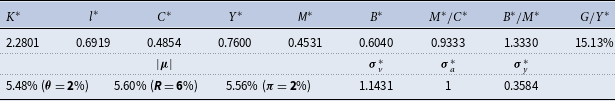
7. Impact of monetary policy on the dynamics of inequality
In Section 5, we showed that monetary policy in isolation has no impact on real aggregate variables, and since the adjustment of the capital stock is the underlying driving force there is no impact on the evolution of the economy. The only response is the initial jump in the price level, which, by instantaneously changing the real stocks of money and bonds, immediately influences wealth and income inequality.Footnote 24
On the other hand, the specification of monetary control – whether setting the money growth rate or pegging the nominal interest rate—will potentially impact the transitional adjustment followed by the economy in response to a real structural change. In the case of real variables, since they are driven solely by differences in the rates of convergence, which have been shown to be only minimally sensitive to monetary policy, the impact is in fact negligible. By contrast, financial variables are also impacted by the initial jump in the price level necessary to sustain intertemporal solvency (as required by (12c) and (9c)), and with more substantial variation across policies, they contribute more significantly to distributional differences.
7.1. Increase in government expenditure (demand increase)
We assume that the economy is initially in steady state and at time 0 government expenditure increases from its benchmark level $G=0.115 (G/Y^{*}=15.13\% )$
to
$G=0.115 (G/Y^{*}=15.13\% )$
to $0.135 (G/Y^{*}=17.34\% )$
.Footnote
25
The resulting changes in key variables are reported in Table 4, with the relevant transitional paths illustrated in Fig. 1.
$0.135 (G/Y^{*}=17.34\% )$
.Footnote
25
The resulting changes in key variables are reported in Table 4, with the relevant transitional paths illustrated in Fig. 1.
Increase in government consumption from 0.115 to 0.135
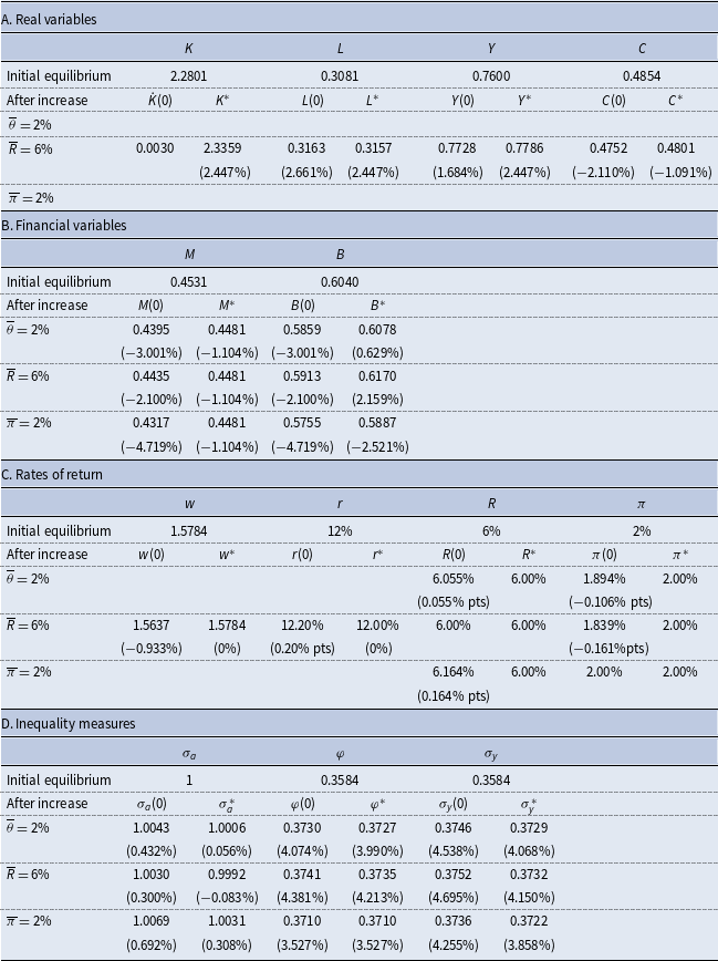
Increase in government expenditure.
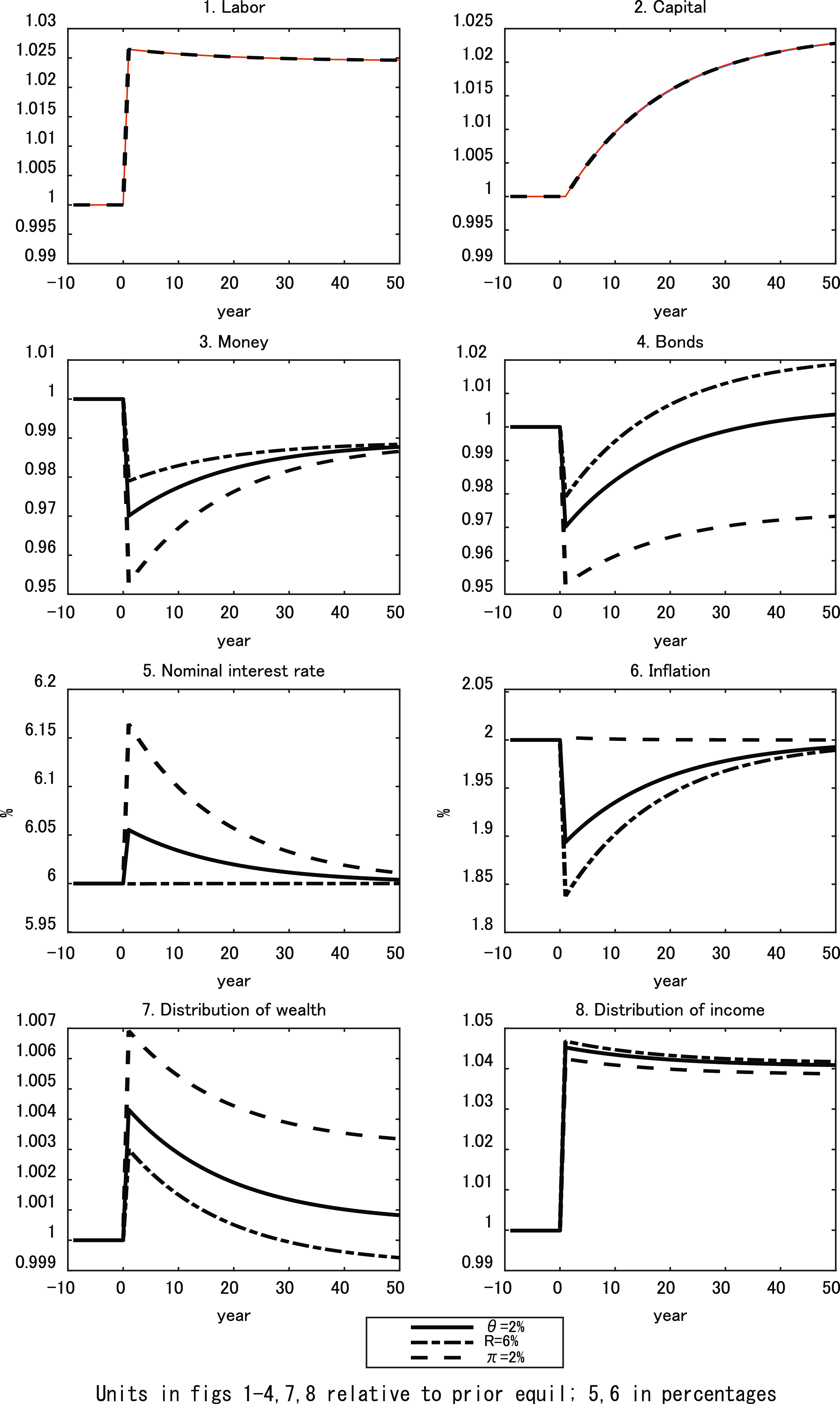
The responses of the aggregate real variables are reported in the first panel and are similar to those obtained by García-Peñalosa and Turnovsky (Reference García-Peñalosa and Turnovsky2011) under lump-sum tax financing and require little further comment. The long-run government expenditure-output multiplier is 0.93, which is consistent with recent empirical estimates that consistently obtain expenditure multipliers below unity,see, for example, Ramey and Zubairy (Reference Ramey and Zubairy2018). The transitional paths followed by $L(t)$
and
$L(t)$
and $K(t)$
are virtually identical for the alternative forms of monetary policy, with the differential rate of convergence (5.48% vs 5.60%) having a negligible impact, see Table 3, Fig. 1a, b.
$K(t)$
are virtually identical for the alternative forms of monetary policy, with the differential rate of convergence (5.48% vs 5.60%) having a negligible impact, see Table 3, Fig. 1a, b.
By contrast, the initial jumps in the price level necessary for the real money stock to attain the stable path (12c), (9c) are 3.0% and 2.1%, respectively (Table 4B, Fig. 1c). These are significant differences and are accounted for by the fact that on impact, the price level must satisfy $P(0)=M_{0}R(0)/\eta C(0)$
, so that
$P(0)=M_{0}R(0)/\eta C(0)$
, so that $d\hat{P}(0)=d\hat{R}(0)-d\hat{C}(0)$
, (where ^ denotes proportional changes) and where
$d\hat{P}(0)=d\hat{R}(0)-d\hat{C}(0)$
, (where ^ denotes proportional changes) and where $d\hat{C}(0)=-2.1\%$
is driven by the government expenditure increase and is independent of monetary policy. The difference is due to the modest increase in the nominal interest rate (from 6.00 to 6.055%) associated with the money growth policy (Table 4C, Fig. 1e).Footnote
26
$d\hat{C}(0)=-2.1\%$
is driven by the government expenditure increase and is independent of monetary policy. The difference is due to the modest increase in the nominal interest rate (from 6.00 to 6.055%) associated with the money growth policy (Table 4C, Fig. 1e).Footnote
26
In both cases, the instantaneous increase in the price level, $P(0)$
, leads to an immediate increase in wealth inequality,
$P(0)$
, leads to an immediate increase in wealth inequality, $\sigma _{a}(0)$
, reflecting the assumption of endowments in (C5). The larger price increase associated with the fixed monetary growth policy, due to the increase in the nominal interest rate, leads to a larger initial increase in wealth inequality (0.43% versus 0.30%, Table 4D). Over time, as capital is accumulated the wage rate increases, while the rate of return to capital declines. This favors the less affluent who are more dependent on income from labor, causing wealth inequality to fall over time. For
$\sigma _{a}(0)$
, reflecting the assumption of endowments in (C5). The larger price increase associated with the fixed monetary growth policy, due to the increase in the nominal interest rate, leads to a larger initial increase in wealth inequality (0.43% versus 0.30%, Table 4D). Over time, as capital is accumulated the wage rate increases, while the rate of return to capital declines. This favors the less affluent who are more dependent on income from labor, causing wealth inequality to fall over time. For $\overline{\theta }=2\%$
, the increase in wealth inequality is reduced to 0.056%, while for
$\overline{\theta }=2\%$
, the increase in wealth inequality is reduced to 0.056%, while for $\overline{R}=6\%$
policy, wealth inequality ends up 0.083% below its pre-shock level (Table 4D). In effect, the initial increase in wealth inequality due to the initial price response channel is gradually offset over time by the decline due to the wage-return to capital channel.
$\overline{R}=6\%$
policy, wealth inequality ends up 0.083% below its pre-shock level (Table 4D). In effect, the initial increase in wealth inequality due to the initial price response channel is gradually offset over time by the decline due to the wage-return to capital channel.
With bonds being denominated in nominal terms, in the short run real bonds drop in the same proportion as do real money balances, namely 3.0% and 2.1%, respectively (Fig. 1d). But with the growth of money supply constrained by policy (2% nominal growth rate in the first case and tracking consumption in the second case) the increase in government expenditure is primarily financed by borrowing, which grows rapidly during the transition (3.63% versus 4.26%, Table 4B). The difference is because pegging the nominal interest rate at $\vec{R}=0.06$
is more constraining on monetary growth and this has consequences for the differences in income inequality.
$\vec{R}=0.06$
is more constraining on monetary growth and this has consequences for the differences in income inequality.
The immediate impact of the increase in government expenditure is to increase employment by 2.66%, leading to an immediate reduction in the wage rate of 0.93% coupled with an increase in the return to capital of 0.20 p.p. (Table 4B). By favoring capital relative to labor, this decline in the wage-return to capital channel favors the more affluent individuals, increasing the “income generating” element, $\varphi$
. In fact, this effect dominates the weak wealth effect, with the result that for the fixed monetary growth policy,
$\varphi$
. In fact, this effect dominates the weak wealth effect, with the result that for the fixed monetary growth policy, $\theta (t)=\overline{\theta }$
, their combined impact is to raise income inequality by 4.54%. Over time, as capital is accumulated, the wage rate increases, the return to capital falls, the initial responses are partially reversed, and the long-run increase in income inequality is reduced to 4.07%. In the case where the monetary authority pegs the nominal interest rate at
$\theta (t)=\overline{\theta }$
, their combined impact is to raise income inequality by 4.54%. Over time, as capital is accumulated, the wage rate increases, the return to capital falls, the initial responses are partially reversed, and the long-run increase in income inequality is reduced to 4.07%. In the case where the monetary authority pegs the nominal interest rate at $R(\mathrm{t})=\overline{R}$
, the impact on income inequality is slightly larger, namely 4.70% in the short run and 4.15% in steady state, see Table 4D.
$R(\mathrm{t})=\overline{R}$
, the impact on income inequality is slightly larger, namely 4.70% in the short run and 4.15% in steady state, see Table 4D.
It is clear that most of the increase in income inequality is due to the real structural change resulting from the expansion in government spending. The contribution to inequality due to the chosen monetary policy is modest, the difference being about 0.16 p.p. (4.54% versus 4.70%) in the immediate increase and 0.08 p.p. (4.07% versus 4.15%) over time. The other point to note from Table 4 is that there is a conflict with respect to the two forms of monetary policy and their respective impacts on wealth and income inequality. While pegging the nominal interest rate reduces the increase in wealth inequality relative to that of targeting the nominal money growth rate, it exacerbates the increase in income inequality. This is true both in the short run and in steady state. But again the differences are small.
7.2. Increase in productivity (supply increase)
Table 5 sets out the analogous effects in the case where TFP increases by 2% from $E=1.2$
to
$E=1.2$
to $1.224.$
In this case, the effects on the real aggregate variables reported in the first panel of Table 5 are similar to those reported by Turnovsky and García-Peñalosa (Reference Turnovsky and García-Peñalosa2008). In contrast to those reported in Table 4, where the increase in government consumption crowds out private consumption, now the increased output can accommodate an increase in private consumption, as well as an increase in leisure (decrease in labor). Over time, as capital is accumulated this growth continues to the new steady state.
$1.224.$
In this case, the effects on the real aggregate variables reported in the first panel of Table 5 are similar to those reported by Turnovsky and García-Peñalosa (Reference Turnovsky and García-Peñalosa2008). In contrast to those reported in Table 4, where the increase in government consumption crowds out private consumption, now the increased output can accommodate an increase in private consumption, as well as an increase in leisure (decrease in labor). Over time, as capital is accumulated this growth continues to the new steady state.
Increase in productivity from 1.20 to 1.224
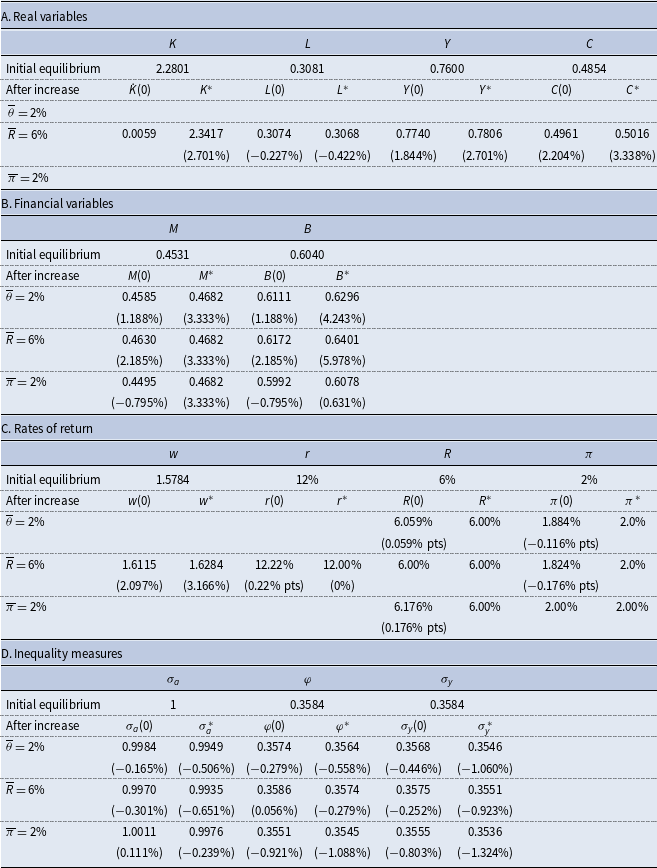
With consumption now increasing instantaneously, the price level must now fall by 1.19% and 2.19%, respectively, under the two forms of monetary policy for the real money stocks to reach their respective stable paths, (12c) and (9c) (Table 5B, Fig. 2c). Again, the difference is due to the modest increase in the nominal interest rate associated with the money growth policy (Fig. 2e).
Increase in productivity.
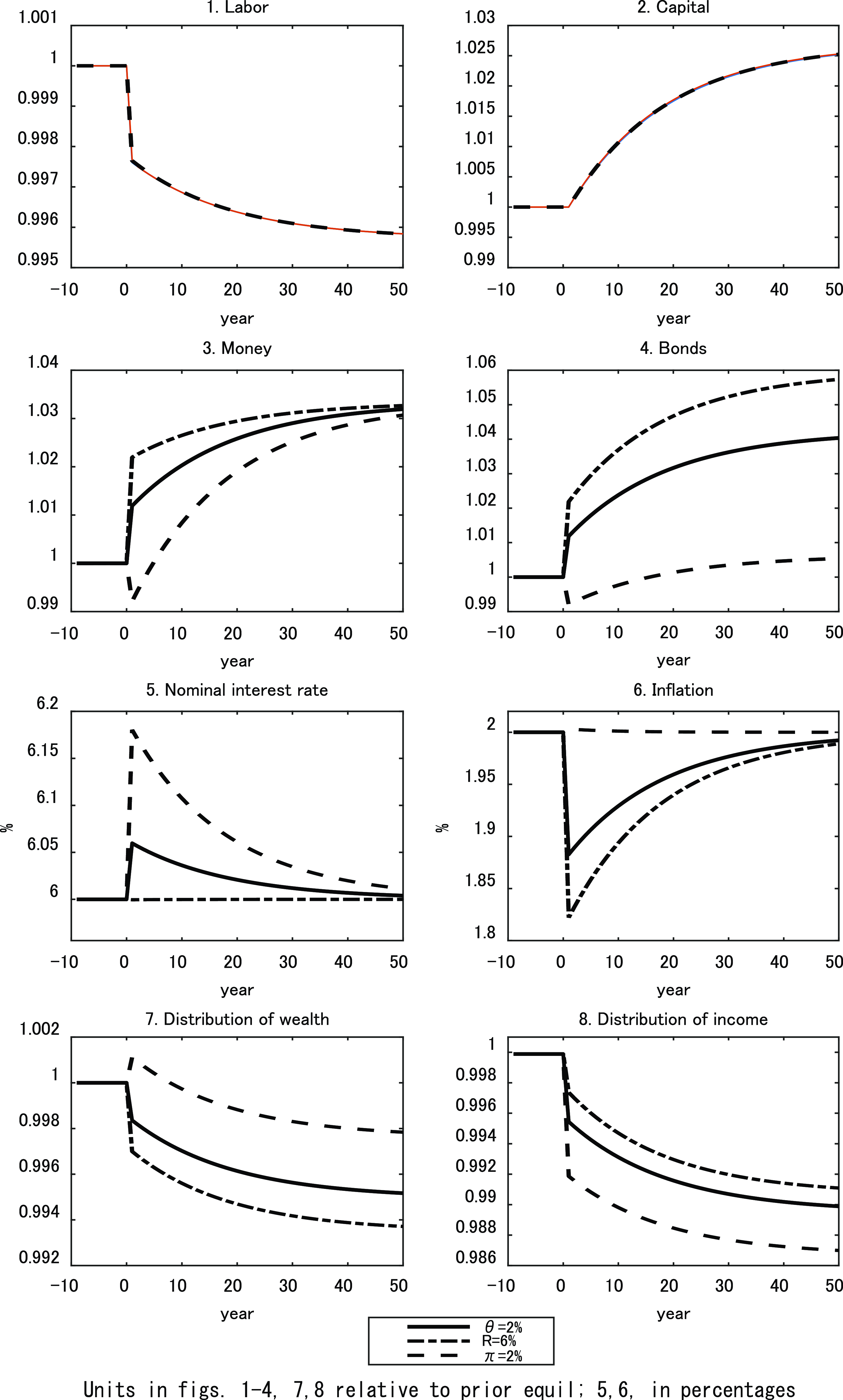
In both cases, the instantaneous decline in the price level leads to an immediate drop in wealth inequality, with the larger price decline associated with the pegged interest rate policy leading to a larger decline in wealth inequality. Over time, as capital is accumulated, the wage rate gradually rises, and the return to capital gradually falls. The same mechanism as before causes wealth inequality to fall gradually over time, adding to the initial decline, with the long run leading to long-run declines in wealth inequality of around 0.51% and 0.65%, respectively (Table 5D).
Analogously to the response to the increase in government spending, the short-run drop in the price level causes bonds to increase immediately in real terms in the same proportion as do real money balances, 1.19% and 2.19%, respectively. Over time, the constraints on the growth of money supply mean that the deficit is financed primarily by bonds which increase by further 3.05% and 3.79%, respectively, during the transition, with long-run increases of 4.24% and 5.98% (Table 5B).
In contrast to the demand shock, the immediate effect of the increase in consumption due to the productivity increase is to increase leisure (an Edgeworth complement), thereby reducing employment by 0.23%, leading to an increase in the wage rate of 2.1%, together with a 0.22 p.p. increase in the return to capital. With both labor and capital experiencing increased rates of return, the impact on the income generating term, $\varphi$
, is weaker and the short-run decline in wealth inequality has a bigger impact on income inequality. As a result, the immediate impact is to reduce income inequality by 0.45% for the fixed monetary growth policy,
$\varphi$
, is weaker and the short-run decline in wealth inequality has a bigger impact on income inequality. As a result, the immediate impact is to reduce income inequality by 0.45% for the fixed monetary growth policy, $\theta (t)=\overline{\theta }$
, and by 0.25% for the
$\theta (t)=\overline{\theta }$
, and by 0.25% for the $R(t)=\overline{R}$
policy. As capital is accumulated, the wage rate increases, while the return to capital falls and in the long run income inequality declines by 1.06% and 0.92%, respectively (Table 5D).
$R(t)=\overline{R}$
policy. As capital is accumulated, the wage rate increases, while the return to capital falls and in the long run income inequality declines by 1.06% and 0.92%, respectively (Table 5D).
Finally, we may note that the conflict between the policies with respect to wealth and income inequality observed with respect to the increase in government expenditure applies here as well, although not as severe. A productivity increase will reduce both wealth and income inequality both in the short run and over time. But the reduction in wealth inequality will be larger if the monetary authority pegs the nominal interest rate, while income inequality will be reduced more if it chooses to maintain the nominal money growth rate.
8. Targeting the inflation rate
We briefly consider a third policy that has been increasingly adopted by a number of central banks, namely targeting the inflation rate, $\pi (t)=\overline{\pi }$
. In this case, the local aggregate dynamics are analogous to those obtained when pegging the nominal interest rate:
$\pi (t)=\overline{\pi }$
. In this case, the local aggregate dynamics are analogous to those obtained when pegging the nominal interest rate:
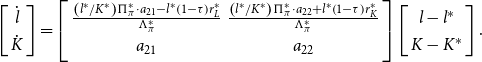 \begin{equation}\left[\begin{array}{c} \dot{l}\\ \dot{K} \end{array}\right]=\left[\begin{array}{cc} \frac{\left(l^{*}/K^{*}\right)\Pi _{\pi }^{*}\cdot a_{21}-l^{*}\left(1-\tau \right)r_{L}^{*}}{\Lambda _{\pi }^{*}} & \frac{\left(l^{*}/K^{*}\right)\Pi _{\pi }^{*}\cdot a_{22}+l^{*}\left(1-\tau \right)r_{K}^{*}}{\Lambda _{\pi }^{*}}\\ a_{21} & a_{22} \end{array}\right]\left[\begin{array}{c} l-l^{*}\\ K-K^{*} \end{array}\right].\end{equation}
with the time path of the real money supply now being determined by
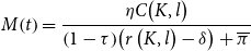 \begin{equation} M\!\left(t\right)=\frac{\eta C\!\left(K,l\right)}{\left(1-\tau \right)\!\left(r\left(K,l\right)-\delta \right)+\overline{\pi }} \end{equation}
while the dynamics of government bonds are now
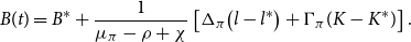 \begin{equation}B(t)=B^{*}+\frac{1}{\mu _{\pi }-\rho +\chi }\left[\Delta _{\pi }\!\left(l-l^{*}\right)+\Gamma _{\pi }(K-K^{*})\right].\end{equation}
subject to the constraints (A11a) and (A11b) and all elements are defined in Appendix A.3.
The impact of the two real shocks on the aggregate and distributional measures is reported in the third rows of the panels in Tables 4 and 5 and their impact on the transitional paths illustrated in Figs. 1 and 2. Recalling the fact that the initial price level must satisfy $d\hat{P}(0)=d\hat{R}(0)-d\hat{C}(0)$
to ensure that the evolution of real money balances must satisfy the consumer transversality condition, the initial price must now accommodate the jump in the real rate of return in order for the inflation rate to remain at its targeted level. In the case of the increase in government expenditure, this now requires a larger increase in the price level of 4.72%, while for the productivity increase the increase in the return to capital dominates that of consumption and the price level must increase (by 0.80%), in contrast to the other two policies.
$d\hat{P}(0)=d\hat{R}(0)-d\hat{C}(0)$
to ensure that the evolution of real money balances must satisfy the consumer transversality condition, the initial price must now accommodate the jump in the real rate of return in order for the inflation rate to remain at its targeted level. In the case of the increase in government expenditure, this now requires a larger increase in the price level of 4.72%, while for the productivity increase the increase in the return to capital dominates that of consumption and the price level must increase (by 0.80%), in contrast to the other two policies.
With inflation targeting causing an increase in government expenditure to generate a larger increase in the initial price level, this leads to a larger initial increase in wealth inequality. In fact, the impact is sufficient that, allowing for the decline in wealth inequality during the transition, targeting the inflation rate causes long-run wealth inequality to rise, rather than fall, as it would if the nominal interest rate were pegged. But it also has a weaker effect on the income generating term, $\varphi (0)$
, increasing income inequality less, than do either of the other two forms of monetary policy. Specifically, compared to pegging the nominal interest rate, it reduces the short-run and long-run increases in income inequality from 4.70% to 4.26% and 4.15% to 3.86%, respectively. An analogous pattern applies following an increase in productivity. In this case, inflation targeting weakens the long-run decline in wealth inequality but strengthens that of income inequality.
$\varphi (0)$
, increasing income inequality less, than do either of the other two forms of monetary policy. Specifically, compared to pegging the nominal interest rate, it reduces the short-run and long-run increases in income inequality from 4.70% to 4.26% and 4.15% to 3.86%, respectively. An analogous pattern applies following an increase in productivity. In this case, inflation targeting weakens the long-run decline in wealth inequality but strengthens that of income inequality.
Table 6 normalizes the relative effects of the two structural shocks on the wealth and income inequality measures, and their sensitivity to alternative forms of monetary policy, in terms of elasticities. This facilitates comparison and suggests the following comparative effects. First, the impact of government consumption on income inequality is insensitive to the three forms of monetary policy. For all three policies, a 10% increase in government expenditure will lead to a short-run increase in income inequality ranging between 2.45% and 2.70%, which declines only slightly over time to between 2.22% and 2.39%.
Elasticities of inequality measures with respect to structural changes
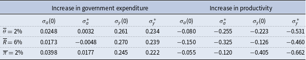
By contrast, both wealth and income inequality are much more sensitive to productivity increases, both over time and with more variation across the accompanying monetary policy. The differences are most striking between pegging the interest rate and inflation targeting. A comparable 10% increase in productivity, with a pegged interest, will lead to a 2.05 p.p. (3.25%–1.20%) larger long-run decline in wealth inequality than does inflation targeting. With respect to income inequality, these relative effects are reversed but the differences are comparable. Inflation targeting reduces long-run income inequality by 2.02 p.p. (6.62%–4.60%) more than if the interest rate is pegged.
9. Relationship to empirical evidence
Much of the recent empirical evidence describing the effects of conventional monetary policy on wealth and income inequality is summarized by Colciago et al. (Reference Colciago, Samarina and de Haan2019), who conclude that it is somewhat mixed. This may reflect the diverse effects of alternative forms of monetary policy adopted by disparate countries of varying stages of development, as well as different historical periods, and is therefore unsurprising.
First, the empirical finding that expansionary monetary policy will reduce wealth inequality seems to be robust across diverse data sets. For example, it is obtained by Doepke and Schneider (Reference Doepke and Schneider2006) using US data, by Meh et al. (Reference Meh, Rios-Rull and Terajima2010) for Canada, and by Adam and Zhu (Reference Adam and Zhu2016) and Hohberger et al. (Reference Hohberger, Priftis and Vogel2019) for the Euro area. While these studies use cross-sectional data across different groups, the mechanism is due to increased inflation eroding the value of assets denominated in nominal terms, favoring poorer borrowers/debtors over more affluent lenders. Our result in Proposition 1 (ii), asserting that an expansionary monetary policy in the form of a reduced nominal interest rate causes an increase in wealth inequality, is entirely consistent with this evidence, although the transfer mechanism is slightly different.Footnote 27 In our setup, there are no private debtors. The transfer in wealth occurs via a discrete unanticipated reduction in the price level, which favors the less affluent, who hold relatively more money over the more affluent who hold relatively more capitalFootnote 28
The empirical relationship between monetary policy and income inequality is more ambiguous. Thus, while Romer and Romer (Reference Romer and Romer1999) and Easterly and Fischer (Reference Easterly and Fischer2001) using cross country data and Inui et al. (Reference Inui, Sudou and Yamada2017) using Japanese data find that an expansionary monetary policy increases income inequality, most studies find that a contractionary policy increases income inequality, see, for example, Coibion et al. (Reference Coibion, Gorodnichenko, Kueng and Soilva2017) for the USA, Muntaz and Theophilopoulou (Reference Muntaz and Theophilopoulou2017) for the UK, Guerello et al. (Reference Guerello2018) and Hohberger et al. (Reference Hohberger, Priftis and Vogel2019) for the Euro area, and Furceri et al. (Reference Furceri, Loungani and Zdzienicka2018) for a range of advanced and emerging economies. From the numerical simulations reported in Table 1, we see that our analysis implies that an expansionary monetary policy can be reconciled with either of these scenarios. Which it is, depends upon the relative size of the wealth effect ( $\sigma _{a}$
) and income-earning effect (
$\sigma _{a}$
) and income-earning effect ( $\varphi$
), and which in turn depends upon the relative structure of the portfolio balance in the economy. Furthermore, in the case when the wealth effect dominates and the higher nominal interest rate target is associated with more income inequality, this also implies a positive association between inflation and income inequality, consistent with Albanesi (Reference Albanesi2007) and Erosa and Ventura (Reference Erosa and Ventura2002).
$\varphi$
), and which in turn depends upon the relative structure of the portfolio balance in the economy. Furthermore, in the case when the wealth effect dominates and the higher nominal interest rate target is associated with more income inequality, this also implies a positive association between inflation and income inequality, consistent with Albanesi (Reference Albanesi2007) and Erosa and Ventura (Reference Erosa and Ventura2002).
We should also point out that our finding that an (exogenous) increase in government consumption expenditure increases income inequality is contrary to recent empirical evidence, see, for example, Agnello and Sousa (Reference Agnello and Sousa2014) and Furceri et al. (Reference Furceri, Ge, Loungani and Melina2022). In response to this potential criticism, we note the following. First, these studies typically include transfers, which we have excluded, but which being disproportionally allocated to the poor, play a substantial inequality-reducing role. Second, by omitting monetary variables, as such empirical studies typically do, they are potentially subject to omitted variable bias. Third, in their extensive literature review, Anderson et al. (Reference Anderson, d’Orey, Duvendack and Esposito2017) stress how the impact of government spending on inequality is highly sensitive to (i) its mode of financing and (ii) its allocation, a finding strongly supported by numerical simulations.Footnote 29 Finally, it is not our objective to track the government spending–inequality relationship per se. Rather, it is to compare the significance of alternative forms of monetary policy in the face of real structural shocks, and for this purpose government spending serves as a convenient form of demand shock.
It is also possible to infer from the simulations the sources of the underlying shocks that are reflected in the observed co-movement between monetary policy and income inequality. For example, comparing the contractionary policy illustrated in Fig. 1e with the increase in income inequality depicted in Fig. 1h suggests that an observed relationship such as this is generated by an underlying demand shock like an increase in government consumption. Similarly, comparing Fig. 2e with the decline in income inequality in Fig. 2h suggests that an observed relationship such as this is compatible with the underlying shock reflecting a productivity increase.
10. Conclusion
This paper has adopted a heterogeneous agent modification of the Sidrauski (Reference Sidrauski1967) model to reconsider the so-called monetary instrument problem initially articulated by Poole (Reference Poole1970), albeit from a longer-run perspective. With flexible prices, the long-run super-neutrality of money with respect to real aggregate measures such as output and capital, previously obtained when setting the nominal money growth rate, also extends to pegging the nominal interest rate. In contrast, the choice of monetary instrument does have consequences for wealth and income inequality, which, furthermore, involve potential conflicts between these two measures. Our main results include the following.
With perfectly flexible prices, a monetary expansion alone has no dynamic consequences. All that occurs is that the price level jumps instantaneously to ensure that real money balances remain consistent with intertemporal solvency. But the form of the monetary expansion matters. If it involves increasing the money growth rate, the instantaneous increase in the price level causes an immediate sustained increase in wealth inequality. If it is a reduction in the nominal interest rate the price level drops and wealth inequality declines. In either case, the price effect also impacts the real income generated by the economy’s productive factors, with the overall effect on income inequality depending upon which effect dominates.
If the economy undergoes some real shock, the accompanying monetary policy will have some impact on the ensuing transitional path. In the case of real variables, this operates entirely through its impact on the speed of convergence and is negligible. With regard to financial variables, the impact also depends upon the initial jumps in the price level. These effects are more substantial across monetary policies, with more significant distributional consequences.
In general, there is a conflict between targeting the money growth rate and pegging the nominal interest, with respect to their relative distributional implications. Maintaining a constant money growth rate will cause a larger increase in wealth inequality but a smaller increase in income inequality following an increase in government expenditure than if the interest rate is pegged. Analogously, pegging the interest rate will lead to a larger decline in wealth inequality but a smaller decline in income inequality, in response to an increase in productivity than if the money growth rate is being maintained. However, the differences are not great and the main impact on both wealth and income inequality is driven by the underlying real shock rather than the accompanying monetary policy.
Finally, we have briefly compared these two policies to the increasingly adopted policy of inflation targeting. This is shown to be the least favorable from the viewpoint of minimizing wealth inequality but the most favorable in terms of reducing income inequality.
This model has been introduced as a benchmark, and to conclude we suggest two directions in which it may be usefully extended. First, the long-run distributional consequences of alternative passive monetary policies—a time horizon over which prices are likely to be flexible—are undoubtedly a relevant concern. Indeed, maintaining a fixed monetary growth rate is at the heart of the position long advocated by Milton Friedman. But it remains unclear what guidance it offers if the objective is one of short-run stabilization. Clearly, it would be of interest to reconsider the distributional consequences of monetary policy from a shorter-run stabilization perspective, when prices are less flexible, and when more activist policies such as a Taylor rule are being implemented.
Second, the underlying property of super-neutrality of money associated with the Sidrauski model is a polar characteristic. Early work by Feldstein (Reference Feldstein1976), Feldstein, Green, and Sheshinski (Reference Feldstein, Green and Sheshinski1978), and others has emphasized how the interaction between the tax structure and inflation is critical in determining the long-run qualitative impact of monetary policy on capital accumulation. The ambiguity of these effects on the aggregate economy suggests that the consequences of this interaction for wealth and income inequality are unclear and merit further detailed study.
Acknowledgements
We are grateful to two anonymous referees for their constructive suggestions. Stephen Turnovsky wishes to acknowledge the Van Voorhis Professorship at the University of Washington for its financial support. Work on this paper was initiated while Yoichi Gokan was visiting the University of Washington. He would like to acknowledge financial support from the JSPS KAKENHI Project (No. 19K01564).
Appendix
A. Local Stability Conditions and Sable Adjustment Paths
A.1. Constant Monetary Growth:
${\theta} =\overline{\theta }$

The fundamental dynamics of the aggregate economy are described by the linearized system, (11), where the previously undefined elements of the matrix are
 $$a_{21}=-F_{L}^{*}-C_{l}^{*}\lt 0 ;\,\, a_{22}=F_{K}^{*}-\delta -C_{K}^{*}.$$
 \begin{equation*}a_{31}=-\eta C_{l}^{*}-M^{*}\left(1-\tau \right)r_{L}^{*}\lt 0;\quad a_{32}=-\eta C_{K}^{*}+M^{*}\!\left(1-\tau \right)r_{K}^{*}\lt 0,\end{equation*}
and $C_{K}^{*}=\frac{s^{*}}{\varepsilon ^{*}}\frac{C^{*}}{K^{*}}\gt 0, C_{l}^{*}=\left(\frac{s^{*}}{\varepsilon ^{*}}\frac{l^{*}}{1-l^{*}}+1\right)\frac{C^{*}}{l^{*}}\gt 0,$
and hence
$C_{K}^{*}=\frac{s^{*}}{\varepsilon ^{*}}\frac{C^{*}}{K^{*}}\gt 0, C_{l}^{*}=\left(\frac{s^{*}}{\varepsilon ^{*}}\frac{l^{*}}{1-l^{*}}+1\right)\frac{C^{*}}{l^{*}}\gt 0,$
and hence $a_{22}=\frac{\rho }{1-\tau }-\frac{s^{*}}{\varepsilon ^{*}}\frac{C^{*}}{K^{*}}$
.
$a_{22}=\frac{\rho }{1-\tau }-\frac{s^{*}}{\varepsilon ^{*}}\frac{C^{*}}{K^{*}}$
.
Under plausible parameterization, certainly met by our benchmark calibration, (11) has a unique stable eigenvalue $\mu _{\theta }\lt 0$
, so that the stable adjustment paths for the key aggregate variables can be expressed as
$\mu _{\theta }\lt 0$
, so that the stable adjustment paths for the key aggregate variables can be expressed as
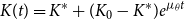 \begin{equation}K(t)=K^{*}+(K_{0}-K^{*})e^{{\mu _{\theta }}t}\end{equation}
 \begin{equation}l(t)=l^{*}+\frac{\mu _{\theta }-a_{22}}{a_{21}}\left(K(t)-K^{*}\right)\end{equation}
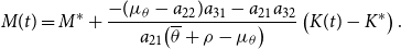 \begin{equation}M(t)=M^{*}+\frac{-(\mu _{\theta }-a_{22})a_{31}-a_{21}a_{32}}{a_{21}\!\left(\overline{\theta }+\rho -\mu _{\theta }\right)}\left(K(t)-K^{*}\right).\end{equation}
Under weak conditions, again satisfied by our calibrations, we can show $\mu _{\theta }-a_{22}\lt 0$
, implying that the coefficients of (A1b) and (A1c) are both positive. Thus, if the economy undergoes an expansion (contraction) in capital, then following initial jumps, leisure and real money balances will both gradually increase (decrease) monotonically, with all variables converging to their respective steady states at the common rate
$\mu _{\theta }-a_{22}\lt 0$
, implying that the coefficients of (A1b) and (A1c) are both positive. Thus, if the economy undergoes an expansion (contraction) in capital, then following initial jumps, leisure and real money balances will both gradually increase (decrease) monotonically, with all variables converging to their respective steady states at the common rate $| \mu _{\theta }| \gt 0$
.
$| \mu _{\theta }| \gt 0$
.
A critical factor determining the evolution of the financial variables is the initial responses of the real stocks of money and bonds, $M(0),B(0)$
, the nominal stocks of which,
$M(0),B(0)$
, the nominal stocks of which, $M^{\prime}(0),B^{\prime}(0)$
, are constrained to gradual adjustments, so that instantaneously they remain at their respective pre-shock levels,
$M^{\prime}(0),B^{\prime}(0)$
, are constrained to gradual adjustments, so that instantaneously they remain at their respective pre-shock levels, $M^{\prime}_{0},B^{\prime}_{0}$
. Writing (A1c) for simplicity as
$M^{\prime}_{0},B^{\prime}_{0}$
. Writing (A1c) for simplicity as $M(t)=M^{*}+\varsigma (K(t)-K^{*})$
, with
$M(t)=M^{*}+\varsigma (K(t)-K^{*})$
, with $K_{0}$
predetermined, the initial jump in the real stock of money consistent with stable adjustment of the economy is
$K_{0}$
predetermined, the initial jump in the real stock of money consistent with stable adjustment of the economy is $dM(0)=dM^{*}-\varsigma dK^{*}$
. With
$dM(0)=dM^{*}-\varsigma dK^{*}$
. With $M(0)=M^{\prime}(0)/P(0) =M^{\prime}_{0}/P(0)$
, the required initial jump in the price level is
$M(0)=M^{\prime}(0)/P(0) =M^{\prime}_{0}/P(0)$
, the required initial jump in the price level is $dP(0)/P(0)\approx -dM(0)/M(0)$
. With
$dP(0)/P(0)\approx -dM(0)/M(0)$
. With $B^{\prime}_{0}$
also being predetermined, the immediate post-shock quantity of real bonds,
$B^{\prime}_{0}$
also being predetermined, the immediate post-shock quantity of real bonds, $B(0)=(B^{\prime}_{0}/M^{\prime}_{0})M(0)$
.
$B(0)=(B^{\prime}_{0}/M^{\prime}_{0})M(0)$
.
To determine the evolution of bonds, we recall the government constraint (7). Using the factor pricing equilibrium conditions, (2), the constant rate of monetary growth policy, $\theta =\overline{\theta }$
, and the adjustment of lump-sum taxes/transfers,
$\theta =\overline{\theta }$
, and the adjustment of lump-sum taxes/transfers, $T=\chi (K+M+B)$
, we may rewrite the constraint as
$T=\chi (K+M+B)$
, we may rewrite the constraint as
 \begin{equation}\dot{B}=G+[(1-\tau )(r-\delta )]B-\overline{\theta }M-\tau (r(K,L)-\delta )K-\tau w(K,L)L-\chi (B+K+M).\end{equation}
Linearizing (A2) around the steady state $(l^{*},K^{*},M^{*},B^{*})$
yields:
$(l^{*},K^{*},M^{*},B^{*})$
yields:
 \begin{align}\dot{B}\!\left(t\right)&=\left(\rho -\chi \right)\!\left(B\!\left(t\right)-B^{*}\right)+\Delta _{\theta }\!\left(l\left(t\right)-l^{*}\right)\nonumber\\[3pt] & \quad+\Gamma _{\theta }(K(t)-K^{*})-(\overline{\theta }+\chi )(M(t)-M^{*}),\end{align}
where:
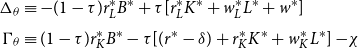 \begin{align*}\Delta _{\theta }&\equiv -(1-\tau )r_{L}^{*}B^{*}+\tau [r_{L}^{*}K^{*}+w_{L}^{*}L^{*}+w^{*}]\\[4pt] \Gamma _{\theta }&\equiv (1-\tau )r_{K}^{*}B^{*}-\tau [(r^{*}-\delta )+r_{K}^{*}K^{*}+w_{K}^{*}L^{*}]-\!\chi\end{align*}
Since $K,l$
, and
$K,l$
, and $M$
converge to their respective steady-state values at the common rate
$M$
converge to their respective steady-state values at the common rate $| \mu _{\theta }|$
, provided
$| \mu _{\theta }|$
, provided $\rho \gt \chi,\text{ and }$
imposing the transversality condition, (5f), the solution to eq. (A3) is
$\rho \gt \chi,\text{ and }$
imposing the transversality condition, (5f), the solution to eq. (A3) is
 \begin{equation}B\!\left(t\right)-B^{*}=\frac{\Delta _{\theta }}{\mu _{\theta }\!-\!\rho +\chi }\left(l\!\left(t\right)-l^{*}\right)+\frac{\Gamma _{\theta }}{\mu _{\theta }\!-\!\rho +\!\chi }\left(K\!\left(t\right)-K^{*}\right)-\frac{\overline{\theta }+\chi }{\mu _{\theta }\!-\!\rho +\chi }\left(M\!\left(t\right)-M^{*}\right).\end{equation}
This describes the dynamics of $B(t)$
in terms of the dynamics of
$B(t)$
in terms of the dynamics of $l(t),\,K(t),\,M(t)$
, but conditional on
$l(t),\,K(t),\,M(t)$
, but conditional on $\chi$
and
$\chi$
and $B^{*}$
, both of which are yet to be determined. These are jointly determined by requiring that (A4) satisfies the initial condition,
$B^{*}$
, both of which are yet to be determined. These are jointly determined by requiring that (A4) satisfies the initial condition, $B(0)=(B^{\prime}_{0}/M^{\prime}_{0})M(0)$
, together with the steady-state government budget constraint, (7), namely:
$B(0)=(B^{\prime}_{0}/M^{\prime}_{0})M(0)$
, together with the steady-state government budget constraint, (7), namely:
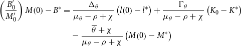 \begin{align} \left(\frac{B^{\prime}_{0}}{M^{\prime}_{0}}\right)M\!\left(0\right)-B^{*}&=\frac{\Delta _{\theta }}{\mu _{\theta }-\rho +\chi }\left(l\!\left(0\right)-l^{*}\right)+\frac{\Gamma _{\theta }}{\mu _{\theta }-\rho +\chi }\left(K_{0}-K^{*}\right)\nonumber \\ & \quad-\frac{\overline{\theta }+\chi }{\mu _{\theta }-\rho +\chi }\left(M\!\left(0\right)-M^{*}\right) \end{align}
 \begin{equation} [\rho -\chi ]B^{*}+G-\overline{\theta }M^{*}-\tau [F(K^{*},L^{*})-\delta K^{*}]+\chi (K^{*}+M^{*})=0 \end{equation}
Thus, (A4) describes a linear approximation to the convergent transitional path for $B(t)$
, where
$B(t)$
, where $\chi$
and
$\chi$
and $B^{*}$
are jointly determined by (A5a) and (A5b).
$B^{*}$
are jointly determined by (A5a) and (A5b).
A.2. Pegging the Nominal Interest Rate: ${R}=\overline{R}$
If the monetary policy maintains a constant nominal interest rate, real money balances are $M=\frac{\eta C\left(K,l\right)}{\overline{R}}$
and the government budget (7) becomes
$M=\frac{\eta C\left(K,l\right)}{\overline{R}}$
and the government budget (7) becomes
 \begin{equation*} \dot{B}=G+\left(1-\tau \right)\!\left(r-\delta \right)B-\frac{\eta }{\overline{R}}\dot{C}\!\left(K,l\right)+\frac{\eta }{\overline{R}}C\!\left(K,l\right)\!\left[\left(1-\tau \right)\!r\!\left(K,L\right)-\overline{R}\right] \end{equation*}
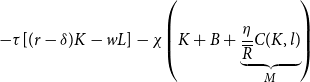 \begin{equation}-\tau [(r-\delta )K-wL]-\chi\! \left(K+B+\underset{M}{\underbrace{\frac{\eta }{\overline{R}}C(K,l)}}\right)\end{equation}
Linearizing the right-hand side of (A6) around the steady state $(l^{*},K^{*},B^{*}),$
as for the case of
$(l^{*},K^{*},B^{*}),$
as for the case of $\theta =\overline{\theta },$
the equilibrium time path for
$\theta =\overline{\theta },$
the equilibrium time path for $B(t)$
becomes
$B(t)$
becomes
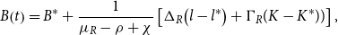 \begin{equation}B\!\left(t\right)=B^{*}+\frac{1}{\mu _{R}-\rho +\chi }\left[\Delta _{R}\!\left(l-l^{*}\right)+\Gamma _{R}(K-K^{*}))\right],\end{equation}
where
 \begin{equation*}\Delta _{R}\equiv -\left(1-\tau \right)\! r_{L}^{*}\left(B^{*}+\frac{\eta }{\overline{R}}C^{*}\right)+\frac{\eta }{\overline{R}}C_{l}^{*}\left(-\mu _{R}+\left(\rho -\overline{R}\right)-\chi \right)+\tau\! \left[r_{L}^{*}K^{*}+w_{L}^{*}L^{*}+w^{*}\right]\end{equation*}
 \begin{equation*}\Gamma _{R}\equiv \left(1-\tau \right)\! r_{K}^{*}\left(B^{*}+\frac{\eta }{\overline{R}}C^{*}\right)+\frac{\eta }{\overline{R}}C_{K}^{*}\left(-\mu _{R}+\left(\rho -\overline{R}\right)-\chi \right)\end{equation*}
 \begin{equation*}-\tau \left[(r^{*}-\delta )+r_{K}^{*}K^{*}+w_{K}^{*}L^{*}\right]-\chi,\end{equation*}
and $B^{*},\chi$
are now determined by
$B^{*},\chi$
are now determined by
 \begin{equation} \left(\frac{B^{\prime}_{0}}{M^{\prime}_{0}}\right)M\!\left(0\right)-B^{*}=\frac{\Delta _{R}}{\mu _{R}-\rho +\chi }\left(l\!\left(0\right)-l^{*}\right)+\frac{\Gamma _{R}}{\mu _{R}-\rho +\chi }\left(K_{0}-K^{*}\right) \end{equation}
 \begin{equation} [\rho +\chi ]B^{*}+G-(\overline{R}-\rho )M^{*}-\tau [F(K^{*},L^{*})-\delta K^{*}]+\chi (K^{*}+M^{*})=0 \end{equation}
A.3. Targeting the Inflation Rate: ${\pi }=\overline{\pi }$
If the monetary policy targets the inflation rate $\pi =\overline{\pi }$
, real money balances can now be expressed as
$\pi =\overline{\pi }$
, real money balances can now be expressed as $M\equiv M(K,l)=\eta C(K,l)/((1-\tau )r(K,L)+\overline{\pi })$
and the government budget (7) as:
$M\equiv M(K,l)=\eta C(K,l)/((1-\tau )r(K,L)+\overline{\pi })$
and the government budget (7) as:
 \begin{equation*} \dot{B}=G+r\!\left(K,L\right)\!B-\underset{\dot{M}}{\underbrace{\left(M_{K}\dot{K}+M_{l}\dot{l}\right)}}-\underset{M}{\underbrace{\frac{\eta }{\left(1-\tau _{K}\right)\! r\!\left(K,L\right)-\delta +\overline{\pi }}C\!\left(K,l\right)}}\overline{\pi } \end{equation*}
 \begin{equation}-\tau [(r-\delta )K-wL]-\chi (B+K+\underset{M}{\underbrace{\frac{\eta }{\left(1-\tau _{K}\right)\! r\!\left(K,L\right)-\delta +\overline{\pi }}C(K,l)}}).\end{equation}
Linearizing the right-hand side of (A9) around the steady state $(l^{*},K^{*},B^{*})$
, the solution becomes
$(l^{*},K^{*},B^{*})$
, the solution becomes
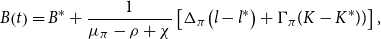 \begin{equation}B\!\left(t\right)=B^{*}+\frac{1}{\mu _{\pi }-\rho +\chi }\left[\Delta _{\pi }\!\left(l-l^{*}\right)+\Gamma _{\pi }(K-K^{*}))\right],\end{equation}
where
 \begin{equation*}\Delta _{\pi }\equiv -\left(1-\tau \right)\!r_{L}^{*}B^{*}-\frac{\eta }{\rho +\overline{\pi }}C_{l}^{*}\!\left(\mu _{\pi }+\overline{\pi }+\chi \right)+\tau r_{L}^{*}K^{*}\end{equation*}
 \begin{equation*}+\tau\! \left(w_{L}^{*}L^{*}+w^{*}\right)-\eta C^{*}\frac{\left(1-\tau \right)\! r_{L}^{*}}{\left(\rho +\overline{\pi }\right)^{2}}\left(\mu _{\pi }+\overline{\pi }+\chi \right),\end{equation*}
 \begin{equation*}\Gamma _{\pi }\equiv \left(1-\tau _{K}\right)\! r_{K}^{*}B^{*}-\frac{\eta }{\rho +\overline{\pi }}C_{K}^{*}\!\left(\mu _{\pi }+\overline{\pi }+\chi \right)-\tau\! \left[\!\left(r_{K}^{*}K^{*}+r^{*}-\delta \right)+ w_{K}^{*}L^{*}\right]\end{equation*}
 \begin{equation*}-\chi +\eta C^{*}\frac{\left(1-\tau \right)r_{K}^{*}}{\left(\rho +\overline{\pi }\right)^{2}}\left(\mu _{\pi }+\overline{\pi }+\chi \right)\end{equation*}
and $B^{*},\chi$
are now determined by
$B^{*},\chi$
are now determined by
 \begin{equation} \left(\frac{B^{\prime}_{0}}{M^{\prime}_{0}}\right)M\!\left(0\right)-B^{*}=\frac{\Delta _{\pi }}{\mu _{\pi }-\rho +\chi }\left(l\left(0\right)-l^{*}\right)+\frac{\Gamma _{\pi }}{\mu _{\pi }-\rho +\chi }\left(K_{0}-K^{*}\right) \end{equation}
 \begin{equation} [\rho +\chi ]B^{*}+G-\overline{\pi }M^{*}-\tau [F(K^{*},L^{*})-\delta K^{*}]+\chi (K^{*}+M^{*})=0 \end{equation}
B. The Dynamics of Relative Wealth and Income
To derive the relative dynamics of individual $i^{\prime}\mathrm{s}$
relative wealth,
$i^{\prime}\mathrm{s}$
relative wealth, $a_{i}(t)\equiv A_{i}(t)/A(t)$
, we sum over the agents’ individual budget constraints, (4), to obtain an expression for the evolution of aggregate wealth,
$a_{i}(t)\equiv A_{i}(t)/A(t)$
, we sum over the agents’ individual budget constraints, (4), to obtain an expression for the evolution of aggregate wealth, $A(t)\equiv K(t)+B(t)+M(t)$
, which we then combine with the individual wealth accumulation eq. (4). This leads to the following relationship determining agent i’s relative rate of wealth accumulation:
$A(t)\equiv K(t)+B(t)+M(t)$
, which we then combine with the individual wealth accumulation eq. (4). This leads to the following relationship determining agent i’s relative rate of wealth accumulation:
 \begin{equation} \dot{a}_{i}=\left(1-\tau \right)\!\frac{w}{A}\left[1-\frac{1+\beta +\eta }{\beta }l_{i}-\left(1-\frac{1+\beta +\eta }{\beta }l\right)a_{i}\right] \end{equation}
We should note that in deriving (B1) we are assuming that $T_{i}/A_{i}=T/A=\chi$
, thus eliminating any (arbitrary) distributional effects of transfers. Recalling eq. (6a),
$T_{i}/A_{i}=T/A=\chi$
, thus eliminating any (arbitrary) distributional effects of transfers. Recalling eq. (6a), $l_{i}/l=\zeta _{i}$
, a constant over time that we obtain from the steady state to (B1):
$l_{i}/l=\zeta _{i}$
, a constant over time that we obtain from the steady state to (B1):
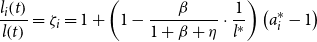 \begin{equation} \frac{l_{i}\!\left(t\right)}{l\!\left(t\right)}=\zeta _{i}=1+\left(1-\frac{\beta }{1+\beta +\eta }\cdot \frac{1}{l^{*}}\right)\left(a_{i}^{*}-1\right) \end{equation}
To analyze the local dynamics of relative wealth, we linearize (B1) around the steady-state $l^{*},K^{*}$
, and
$l^{*},K^{*}$
, and $a_{i}^{*}$
. Using (17), the bounded solution for agent i’s relative share of wealth,
$a_{i}^{*}$
. Using (17), the bounded solution for agent i’s relative share of wealth, $a_{i}(t)$
, is
$a_{i}(t)$
, is
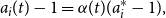 \begin{equation}a_{i}(t)-1=\alpha (t)(a_{i}^{*}-1),\end{equation}
where $\alpha\! \left(t\right)\equiv 1+\left(\frac{\left(1-\tau \right)w^{*}}{A^{*}}\left[1-\frac{l\left(t\right)}{l^{*}}\right]\right)\left(\frac{\left(1-\tau \right)w^{*}}{A^{*}}\left[\frac{l^{*}}{\upsilon }-1\right]-\mu \right)^{-1}$
Setting $t=0$
in (B3) yields
$t=0$
in (B3) yields $a_{i}(0)-1=\alpha (0)(a_{i}^{*}-1)$
, which, combined with (B3), implies
$a_{i}(0)-1=\alpha (0)(a_{i}^{*}-1)$
, which, combined with (B3), implies
 \begin{equation} a_{i}\!\left(t\right)-1=\frac{\alpha\! \left(t\right)}{\alpha\! \left(0\right)}\left(a_{i}\!\left(0\right)-1\right) \end{equation}
Let $t\rightarrow \infty$
, we see that agent
$t\rightarrow \infty$
, we see that agent $i^{\prime}\mathrm{s}$
relative wealth in steady state,
$i^{\prime}\mathrm{s}$
relative wealth in steady state, $a_{i}^{*},$
is
$a_{i}^{*},$
is
 \begin{equation} a_{i}^{*}-1=\frac{1}{\alpha\! \left(0\right)}\left(a_{i}\!\left(0\right)-1\right) \end{equation}
where the individual’s initial relative wealth, $a_{i}(0)$
, is endogenous.
$a_{i}(0)$
, is endogenous.
As noted, to determine the agent’s relative income we need to determine his relative wealth position in real money balances and income-earning assets. Using (7a), (D.2), and (D.3), we can relate agent $i^{\prime}$
s relative position in real money balances to his relative wealth:
$i^{\prime}$
s relative position in real money balances to his relative wealth:
 \begin{equation} \frac{M_{i}}{M}-1=\left(1-\frac{\upsilon }{l^{*}}\right)\frac{1}{\alpha\! \left(t\right)}\cdot \left[a_{i}\!\left(t\right)-1\right] \end{equation}
With capital and bonds yielding the same rate of return, and in the absence of risk, investors view these two assets as perfect substitutes, enabling us to characterize their composite distribution. Letting $V_{i}\equiv B_{i}+K_{i}$
and
$V_{i}\equiv B_{i}+K_{i}$
and $V\equiv B+K$
, so that
$V\equiv B+K$
, so that $v_{i}-1\equiv (V_{i}/V)-1$
, and using (B5) in conjunction with the definition of relative wealth, we can show:
$v_{i}-1\equiv (V_{i}/V)-1$
, and using (B5) in conjunction with the definition of relative wealth, we can show:
 \begin{equation} v_{i}(t)-1=\omega (t)(a_{i}(t)-1) \end{equation}
where:
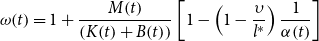 \begin{equation*} \omega\! \left(t\right)=1+\frac{M\!\left(t\right)}{\left(K\!\left(t\right)+B\!\left(t\right)\right)}\left[1-\left(1-\frac{\upsilon }{l^{*}}\right)\frac{1}{\alpha\! \left(t\right)}\right] \end{equation*}
which expresses the agent’s relative position of the composite income-earning asset, ( $B(t)+K(t)$
) in terms of his overall relative position in wealth.
$B(t)+K(t)$
) in terms of his overall relative position in wealth.
As noted in the text, we focus on before-tax personal income, which, for individual i is:
 \begin{equation} Y_{i}(t)=r(t)V_{i}(t)+w(t)L{i}^{}{(}{}t) \end{equation}
while the average economy-wide before-tax personal income is
 \begin{equation} Y(t)=r(t)V(t)+w(t)L(t) \end{equation}
Dividing (B7a) by (B7b), and using (B2) and (B5), the relative before-tax income of agent i, $y_{i}(t)\equiv Y_{i}(t)/Y(t)$
, can be expressed as
$y_{i}(t)\equiv Y_{i}(t)/Y(t)$
, can be expressed as
 \begin{equation} y_{i}(t)-1=\varphi (t)[a_{i}(t)-1] \end{equation}
where:
 \begin{equation} \varphi\! \left(t\right)\equiv \frac{r\!\left(t\right)V\!\left(t\right)}{r\!\left(t\right)V\!\left(t\right)+w\!\left(t\right)L\!\left(t\right)}\omega\! \left(t\right)-\frac{w\!\left(t\right)l\!\left(t\right)}{r\!\left(t\right)V\!\left(t\right)+w\!\left(t\right)L\!\left(t\right)}\left(1-\frac{\upsilon }{l^{*}}\right)\frac{1}{\alpha\! \left(t\right)} \end{equation}
Substituting for $\omega (t)$
and using the definitions
$\omega (t)$
and using the definitions $A(t)\equiv K(t)+B(t)+M(t)=V(t)+M(t)$
this can be expressed as in (20b) in the text.
$A(t)\equiv K(t)+B(t)+M(t)=V(t)+M(t)$
this can be expressed as in (20b) in the text.
C. Determination of Initial Price and Initial Wealth Inequality
Following a shock, the price level undergoes an initial jump, $dP(0)$
. This is to ensure that the real money stock,
$dP(0)$
. This is to ensure that the real money stock, $M(0)$
, jumps onto the stable path, (9b), and depends upon the specific shock driving the aggregate dynamics. To determine the effect on individual i’s initial relative wealth,
$M(0)$
, jumps onto the stable path, (9b), and depends upon the specific shock driving the aggregate dynamics. To determine the effect on individual i’s initial relative wealth, $a_{i}(0)$
, and the impact effect on initial wealth inequality,
$a_{i}(0)$
, and the impact effect on initial wealth inequality, $\sigma _{a}(0)$
, we begin by writing
$\sigma _{a}(0)$
, we begin by writing
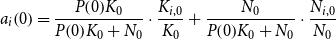 \begin{equation} a_{i}\!\left(0\right)=\frac{P\!\left(0\right)\! K_{0}}{P\!\left(0\right)\! K_{0}+N_{0}}\cdot \frac{K_{i,0}}{K_{0}}+\frac{N_{0}}{P\!\left(0\right)\! K_{0}+N_{0}}\cdot \frac{N_{i,0}}{N_{0}} \end{equation}
where $N_{0}\equiv M^{\prime}_{0}+B^{\prime}_{0},\,\,\,N_{i,0}\equiv M^{\prime}_{i,0}+B^{\prime}_{i,0}$
and primes denote nominal quantities. From (C1) we see that the effect of the initial jump in
$N_{0}\equiv M^{\prime}_{0}+B^{\prime}_{0},\,\,\,N_{i,0}\equiv M^{\prime}_{i,0}+B^{\prime}_{i,0}$
and primes denote nominal quantities. From (C1) we see that the effect of the initial jump in $P(0)$
from its prior level, on the agent’s relative wealth, is
$P(0)$
from its prior level, on the agent’s relative wealth, is
 \begin{equation} \frac{da_{i}\!\left(0\right)}{a_{i}\!\left(0\right)}=\left[\frac{P\!\left(0\right)\! K_{i,0}}{P\!\left(0\right)\! K_{i,0}+N_{i,0}}-\frac{P\!\left(0\right)\! K_{0}}{P\!\left(0\right)\! K_{0}+N_{0}}\right]\frac{dP\!\left(0\right)}{P\!\left(0\right)} \end{equation}
If an agent’s endowment portfolio of assets coincides with the economy-wide endowment, the term in parentheses is zero and $da_{i}(0)=0$
, independent of the price change. Otherwise, if the agent’s portfolio is weighted more (less) toward the real asset (capital),
$da_{i}(0)=0$
, independent of the price change. Otherwise, if the agent’s portfolio is weighted more (less) toward the real asset (capital), $dP(0)\gt 0$
is associated with
$dP(0)\gt 0$
is associated with $da_{i}(0)\gt 0(da_{i}(0)\lt 0)$
.
$da_{i}(0)\gt 0(da_{i}(0)\lt 0)$
.
To determine the impact on overall initial wealth inequality, we rewrite (C1), as:
 \begin{equation} a_{i}\!\left(0\right)-1=\frac{P\!\left(0\right)\! K_{0}}{P\!\left(0\right)\! K_{0}+N_{0}}\left(k_{i,0}-1\right)+\frac{N_{0}}{P\!\left(0\right)\! K_{0}+N_{0}}\left(n_{i,0}-1\right) \end{equation}
where $n_{i,0}\equiv N_{i,0}/N_{0}$
. Denoting the ratio of nominal assets,
$n_{i,0}\equiv N_{i,0}/N_{0}$
. Denoting the ratio of nominal assets, $N_{0}$
, to total nominal wealth by
$N_{0}$
, to total nominal wealth by $\varpi \equiv N_{0}/(P(0)K_{0}+N_{0})$
, the standard deviation of initial wealth across agents following a shock is
$\varpi \equiv N_{0}/(P(0)K_{0}+N_{0})$
, the standard deviation of initial wealth across agents following a shock is
 \begin{equation} \sigma _{a}(0)=[(1-\varpi )^{2}\sigma _{k,0}^{2}+2(1-\varpi )\varpi \sigma _{k,0}\sigma _{n,0}v +\varpi ^{2}\sigma _{n,0}^{2}]^{1/2} \end{equation}
From the definition of $\varpi, d\varpi /\varpi =-(1-\varpi )[dP(0)/P(0)]$
, and hence, the effect of the change in price from its pre-shock level on initial wealth inequality is
$\varpi, d\varpi /\varpi =-(1-\varpi )[dP(0)/P(0)]$
, and hence, the effect of the change in price from its pre-shock level on initial wealth inequality is
 \begin{equation} \frac{d\sigma _{a}\!\left(0\right)}{\sigma _{a}\!\left(0\right)}=\left[\left(1-\varpi \right)\sigma _{k,0}^{2}-\left(1-2\varpi \right)\sigma _{k,0}\sigma _{n,0}\nu -\varpi \sigma _{n,0}^{2}\right]\frac{\left(1-\varpi \right)\!\varpi }{\sigma _{a}^{2}\!\left(0\right)}\left[\frac{dP\!\left(0\right)}{P\!\left(0\right)}\right] \end{equation}
From eq. (C5), we see that the impact of the initial price on initial wealth inequality depends upon the total relative endowments of nominal versus real assets, $\varpi$
, and the standard deviations,
$\varpi$
, and the standard deviations, $\sigma _{k,0},\sigma _{n,0}$
and correlation,
$\sigma _{k,0},\sigma _{n,0}$
and correlation, $\nu$
, of their distributions across agents. Under plausible conditions, the term in parentheses in (C5) can be shown to be positive. With
$\nu$
, of their distributions across agents. Under plausible conditions, the term in parentheses in (C5) can be shown to be positive. With $-1\lt \nu \lt 1$
, we can show that weak conditions that ensure this to be so are (i)
$-1\lt \nu \lt 1$
, we can show that weak conditions that ensure this to be so are (i) $\varpi \lt 1/2$
, that is, that the economy-wide endowment of real assets (capital) exceeds that of nominal (financial) assets, and (ii)
$\varpi \lt 1/2$
, that is, that the economy-wide endowment of real assets (capital) exceeds that of nominal (financial) assets, and (ii) $\sigma _{n,0}\leq \sigma _{k,0}$
, nominal asserts are less unequally endowed across agents than are real assets. In the absence of specific information pertaining to
$\sigma _{n,0}\leq \sigma _{k,0}$
, nominal asserts are less unequally endowed across agents than are real assets. In the absence of specific information pertaining to $\sigma _{k,0},\sigma _{n,0},\,\,\,\mathrm{or}\,\,\nu$
our simulations assume
$\sigma _{k,0},\sigma _{n,0},\,\,\,\mathrm{or}\,\,\nu$
our simulations assume $\sigma _{k,0}=\sigma _{n,0},\,\,\nu =0$
, when (C5) simplifies to
$\sigma _{k,0}=\sigma _{n,0},\,\,\nu =0$
, when (C5) simplifies to
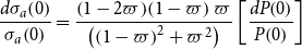 \begin{equation} \frac{d\sigma _{a}\!\left(0\right)}{\sigma _{a}\!\left(0\right)}=\frac{\left(1-2\varpi \right)\!\left(1-\varpi \right)\varpi }{\left(\left(1-\varpi \right)^{2}+\varpi ^{2}\right)}\left[\frac{dP\!\left(0\right)}{P\!\left(0\right)}\right] \end{equation}
While these restrictions are arbitrary, the results are fairly robust with regard to modest relaxation with regard to these distributional parameters.


 Open access