





Impact statement
In fluid dynamics, data assimilation integrates experimental measurements with low-fidelity simulations to address the shortcomings of both. This work extends the recent work using physics-informed neural networks (PINNs) to experimental datasets of higher Reynolds number stalled airfoil flows. Using our proposed methodology, we have shown the ability of PINNs to reconstruct the entire flow field from sparse measurements and predict key surface quantities.
1. Introduction
Particle image velocimetry (PIV) enables high-quality multi-component flow velocity measurements for a variety of flows. However, there are limitations with dynamic range, both in terms of scales (ratio of largest size to the smallest size) and velocities (largest to the smallest component), as well as obtaining data in the near-wall region. Moreover, as with any experimental technique, noise and uncertainty are present in the data and vary across the captured domain. These issues can be addressed using high-fidelity computational fluid dynamics (CFD) simulation methods such as large eddy simulation (LES) or direct numerical simulation (DNS), but such methods become intractable at higher Reynolds numbers (Doran, Reference Doran and Doran2013). RANS simulations reduce the computational cost but sacrifice accuracy in the final solution for flows with large pressure gradients and separation. PINNs provide an alternative method for solving the broader data assimilation problem of noise reduction, expanding the field of view, and obtaining reliable secondary quantities. The objective of this work is to achieve this from sparse experimental PIV measurements using PINNs.
Initially proposed by Raissi et al. (Reference Raissi, Perdikaris and Karniadakis2019), PINNs utilize modern advancements in machine learning and neural networks to directly solve partial differential equations (PDEs) by leveraging automatic differentiation to compute the necessary gradients. At its core, the assumption is that a neural network can approximate a solution to a non-linear function, in this case, the RANS equations (Hornik et al., Reference Hornik, Stinchcombe and White1989). The differentiating factor between PINNs and CFD is that PINNs directly compare predictions to reference data at discrete locations to find a solution for the entire field.
One of the foundational papers on the PINN methodology and the application of sparse reference data to reconstruct the mean flow quantities is by Sliwinski and Rigas (Reference Sliwinski and Rigas2023). In this work, they investigated predicting a time-averaged cylinder flow at Reynolds number of Re = 150 from a sparse sampling of a DNS solution. To do so, they used the forcing representation of the Reynolds stresses initially proposed by Foures et al. (Reference Foures, Dovetta, Sipp and Schmid2014) to reduce the discrepancy between unknowns and equations to solve. By decomposing the forcing via the Helmholtz decomposition, the disparity of unknowns to equations is one. Even with an underdetermined system of equations, this PINN formulation yielded improved predictions of the mean velocity field with uniformly sparse data of two points per cylinder diameter. Furthermore, the results highlighted the ability of PINNs to work with sparse and noisy data. However, the authors noted in the conclusions that there were small reconstruction errors at the surface of the cylinder.
An alternative reconstruction method, proposed by von Saldern et al. (Reference von Saldern, Reumschüssel, Kaiser, Sieber and Oberleithner2022), uses the Boussinesq approximation (Boussinesq, Reference Boussinesq1877) and seeks to find the eddy viscosity
$ {\nu}_t $
 that minimizes the mismatch between the experimental data and the RANS solution. The authors used this approach to assimilate a swirling, turbulent jet flow from a reference stereo-PIV dataset. The network implicitly derived an eddy viscosity model from the data, which, when used to calculate the Reynolds stresses, had good agreement with the data.
Rather than allow the PINN to indirectly construct a model for computing the Reynolds stresses, Patel et al. (Reference Patel, Mons, Marquet and Rigas2024) extended the equations to include the Spalart–Allmaras turbulence model, in which an additional variable,
$ \tilde{\nu} $
 , is solved. This variable represents a modified form of the turbulent kinematic viscosity and is used to compute the eddy viscosity term,
$ {\nu}_t $
, is solved. This variable represents a modified form of the turbulent kinematic viscosity and is used to compute the eddy viscosity term,
$ {\nu}_t $
 , which accounts for the additional momentum transfer induced by turbulent fluctuations. This formulation does not change the disparity of unknowns to equations but provides further constraints on the PINN. Patel et al. (Reference Patel, Mons, Marquet and Rigas2024) applied their formulation to a periodic hill case for a Reynolds number of Re = 5600. The addition of a turbulence model improved flow predictions throughout the domain, particularly in the near-wall region and at the separation point (Patel et al., Reference Patel, Mons, Marquet and Rigas2024). Others have also implemented a turbulence model into the PINNs equation formulation. Pioch et al. (Reference Pioch, Harmening, Müller, Peitzmann, Schramm and Moctar2023) applied a k-
$ \omega $
, which accounts for the additional momentum transfer induced by turbulent fluctuations. This formulation does not change the disparity of unknowns to equations but provides further constraints on the PINN. Patel et al. (Reference Patel, Mons, Marquet and Rigas2024) applied their formulation to a periodic hill case for a Reynolds number of Re = 5600. The addition of a turbulence model improved flow predictions throughout the domain, particularly in the near-wall region and at the separation point (Patel et al., Reference Patel, Mons, Marquet and Rigas2024). Others have also implemented a turbulence model into the PINNs equation formulation. Pioch et al. (Reference Pioch, Harmening, Müller, Peitzmann, Schramm and Moctar2023) applied a k-
$ \omega $
 , as well as other mixing length-based models, to a backwards-facing step case at a Reynolds number of Re = 5100 and found good agreement with reference data but noted the difficulty in training stability, resulting in unphysical predictions.
In many of these cases, the reference data used to train the PINN originated from a DNS solution as opposed to experimental measurements. Relatively few have directly integrated raw experimental data into PINNs. One example by Steinfurth and Weiss (Reference Steinfurth and Weiss2024) trained a PINN model using planar PIV collected at multiple planes, surface pressure, and wall shear-stress measurements from a backwards-facing ramp model. These measurements were aggregated and used to train a three-dimensional PINN with a mixing length model to approximate the Reynolds shear stresses instead of one of the aforementioned eddy viscosity models. When training a PINN, the loss function incorporates evaluations at both data points from a reference data set and randomly generated collocation points. In the context of PINNs, collocation points are equivalent to cells in a CFD solver, which provide locations to assess how closely the predicted quantities fit the governing equations and boundary conditions. In Steinfurth and Weiss (Reference Steinfurth and Weiss2024), with the amount of data points in the domain, they required much fewer additional collocation points to evaluate the physics loss and boundary conditions. Furthermore, the authors found that the predictions improved overall by significantly suppressing the contribution of the physics loss to the total loss. This approach lends itself to a data-rich assimilation problem and was shown to be effective, in particular, for fixing stitching errors in the reference PIV dataset. Other attempts to integrate a turbulence model within a PINN include the work by Villié et al. (Reference Villié, Schmitter, von Saldern, Demange and Oberleithner2025). Here, the authors applied a Spalart–Allmaras turbulence model to enhance experimental MRI measurements of a transitioning stenosis flow. The PINN reduced errors associated with the measurement technique in the velocity components and found reasonable agreement with the simulations for other quantities, such as pressure and Reynolds stresses.
Klopsch et al. (Reference Klopsch, Fuchs, Rigas, Oberleithner and von Saldern2025) expanded the work of Patel et al. (Reference Patel, Mons, Marquet and Rigas2024) to apply PINNs with the same formulation of the Spalart–Allmaras equations, but to experimental PIV measurements of a flow past a Boeing Gaussian Bump at two Reynolds numbers of Re =
$ 1\times {10}^6 $
 and
$ 2\times {10}^6 $
and
$ 2\times {10}^6 $
 , respectively. These two Reynolds numbers represent a mostly attached and a fully separated flow, respectively. The authors provided windows of time-averaged PIV data at different streamwise locations along the Gaussian bump. The PINN then reconstructed the continuous velocity field across the domain, alongside predicting the pressure and eddy viscosity fields. Whilst the obtained fields were physically consistent, it was noted that the assimilated eddy viscosity did not fully conform to the Spalart-Allmaras model.
For most existing PINN methodologies, the network weights and biases are initiated randomly and sampled from a distribution based on the activation function used. In the broader machine learning community, it is common to start from a pre-trained model developed to solve a similar task, for example, in computer vision or text-based tasks (Too et al., Reference Too, Yujian, Njuki and Yingchun2019; Ziegler et al., Reference Ziegler, Stiennon, Wu, Brown, Radford, Amodei, Christiano and Irving2019). This process, known as transfer learning, involves fine-tuning a model through additional training with a new, domain-specific dataset. The benefit of this is a reduction of computational cost by reducing the subsequent training time and often improving results over building a model directly by initiating training from a more informed starting set of network parameters (Torrey and Shavlik, Reference Torrey and Shavlik2010; Weiss et al., Reference Weiss, Khoshgoftaar and Wang2016; Chakraborty, Reference Chakraborty2021).
In this work, we apply transfer learning to PINNs such that they reconstruct mean flows from limited experimental measurements. The PINN enforces the incompressible RANS equations with a Spalart–Allmaras turbulence model. It is first trained on a baseline RANS simulation such that it successfully predicts all states, including the eddy viscosity and pressure. The PINN is subsequently transferred to sub-sampled LES and PIV data to reconstruct all states inside and outside the experimental domain. The key idea behind this proposed method is to form stronger priors, in the form of better estimates of the networks’ initial parameters, from the RANS data before training with sparse experimental data. The rest of the paper is organized as follows. In Section 2, we detail the PINN formulation and specifics of the configuration for this work. Section 3 outlines the new training methodologies as well as the datasets used throughout this work. Section 4 showcases the results and discusses some of the fundamental challenges when using PINNs in this application. Section 5 summarizes the findings from applying these new methodologies and discusses some potential extensions.
2. PINN and problem setup
Like many other data assimilation techniques, the PINN framework fits sparse measurements to a set of governing equations (Raissi et al., Reference Raissi, Perdikaris and Karniadakis2019). Given that the scope of this work is to assimilate experimental PIV measurements in 2D, we construct the physics loss of the PINN from the 2D RANS equations. The methodology presented here builds upon recent work by Sliwinski and Rigas (Reference Sliwinski and Rigas2023) and Patel et al. (Reference Patel, Mons, Marquet and Rigas2024). Section 2.1 focuses on the governing equations used in this work, with Section 2.2 describing how these equations integrate within the loss function. Section 2.3 outlines the extension to boundary conditions through the application of hard constraints. Section 2.4 covers the details of the network architecture, and Section 2.5 aggregates the various aspects of the PINN and provides specific information about the implementation for the work presented through the result sections.
2.1. Governing equations
For a mean flow problem, we can apply the Reynolds decomposition to split the flow quantities into their respective steady (
$ \overline{U_i},\overline{P} $
 ) and unsteady (
$ {u}_i^{\prime },{p}^{\prime } $
) and unsteady (
$ {u}_i^{\prime },{p}^{\prime } $
 ) parts. Once substituted into the Navier–Stokes equations and averaged in time, we obtain the RANS equations

where
$ \overline{U_i} $
 is the mean velocity,
$ P $
is the mean velocity,
$ P $
 is pressure,
$ \rho $
is pressure,
$ \rho $
 is density and
$ \nu $
is density and
$ \nu $
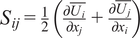
 is kinematic viscosity. The two remaining terms represent the strain rate tensor,
$ {S}_{ij}=\frac{1}{2}\left(\frac{\partial \overline{U_i}}{\partial {x}_j}+\frac{\partial \overline{U_j}}{\partial {x}_i}\right) $
is kinematic viscosity. The two remaining terms represent the strain rate tensor,
$ {S}_{ij}=\frac{1}{2}\left(\frac{\partial \overline{U_i}}{\partial {x}_j}+\frac{\partial \overline{U_j}}{\partial {x}_i}\right) $
 , and the divergence of the Reynolds stress tensor
$ \overline{u_i^{\prime }{u}_j^{\prime }} $
, and the divergence of the Reynolds stress tensor
$ \overline{u_i^{\prime }{u}_j^{\prime }} $
 . For a 2D problem, Equation 2.1 provides three equations with six unknowns, creating an under-determined system to solve. This issue is known as the closure problem. Within the turbulence modeling and data assimilation communities, numerous approaches, with varying levels of complexity, have been proposed as solutions to the closure problem. In the work presented here, we will consider two approaches: one model-free and the other modeled using a Spalart–Allmaras turbulence model.
For the model-free approach, we allow the PINN to determine the Reynolds stresses through the training process. In this case, the output layer would require a node for each component of the Reynolds stress tensor. However, it is more effective to reduce the disparity between equations and unknowns (Sliwinski and Rigas, Reference Sliwinski and Rigas2023). Initially proposed by Foures et al. (Reference Foures, Dovetta, Sipp and Schmid2014), the divergence of the Reynolds stresses can be represented as a forcing term,
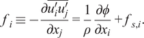
Applying the Helmholtz decomposition to
$ {f}_i $
 results in two terms: a potential,
$ \phi $
results in two terms: a potential,
$ \phi $
 and solenoidal,
$ {f}_{s,i} $
and solenoidal,
$ {f}_{s,i} $
 , component. By combining Equation 2.1 with Equation 2.2, we can derive the RANS with forcing (RANS-F) equations, given by

As the forcing term,
$ {f}_{s,i} $
 , is solenoidal, we can also specify that the forcing must be divergence-free. Additionally, to reduce the number of unknowns, we can combine the pressure with
$ \phi $
, is solenoidal, we can also specify that the forcing must be divergence-free. Additionally, to reduce the number of unknowns, we can combine the pressure with
$ \phi $
 as a single term (
$ \overline{P}-\phi $
as a single term (
$ \overline{P}-\phi $
 ). The resulting system remains under-determined, but the number of unknowns has been reduced to five with four equations. The reduction in unknowns, while attempting to mitigate one problem, creates the issue that the pressure remains coupled with
$ \phi $
). The resulting system remains under-determined, but the number of unknowns has been reduced to five with four equations. The reduction in unknowns, while attempting to mitigate one problem, creates the issue that the pressure remains coupled with
$ \phi $
 . Therefore, even with a fully known velocity field and subsequently making the system determined, the predicted pressure may not be equivalent to the true pressure as the influence of
$ \phi $
. Therefore, even with a fully known velocity field and subsequently making the system determined, the predicted pressure may not be equivalent to the true pressure as the influence of
$ \phi $
 is unknown (Foures et al., Reference Foures, Dovetta, Sipp and Schmid2014; Sliwinski and Rigas, Reference Sliwinski and Rigas2023).
The second approach to solving the closure problem is empirically modeling the Reynolds stresses through a turbulence model. This approach is commonly seen in numerical solvers and relies on the Boussinesq approximation to relate the Reynolds stresses to a combination of the mean velocity gradients and a modeled eddy viscosity term,
$ {\nu}_t $
 , as given by

for an incompressible flow, where
$ k $
 is the turbulent kinetic energy and
$ {\delta}_{ij} $
is the turbulent kinetic energy and
$ {\delta}_{ij} $
 is the Kronecker delta (Boussinesq, Reference Boussinesq1877). In this work, following recent literature, a Spalart–Allmaras (SA) turbulence model was selected to model the eddy viscosity term (Franceschini et al., Reference Franceschini, Sipp and Marquet2020; Patel et al., Reference Patel, Mons, Marquet and Rigas2024). For a mean flow problem, the transport equation simplifies to,

This formulation provides one additional unknown,
$ \tilde{\nu} $
 , and one additional equation (Spalart and Allmaras, Reference Spalart and Allmaras1994). For the Spalart–Allmaras transport equation, Equation 2.5, the mean velocity gradients predominantly drive the production and destruction of eddy viscosity through the domain. Therefore, for the PINN, the sensitivity to the mean velocity gradients is increased to solve this equation correctly. The following equation relates this additional term to the eddy viscosity in the momentum equations


where
$ {c}_{v1}=7.3 $
 . With this approach, the forcing,
$ {f}_i $
. With this approach, the forcing,
$ {f}_i $
 , from Equation 2.2, will still represent the divergence of the Reynolds stresses. The key difference is that the forcing term is a corrective forcing,
$ {f}_{c,i} $
, from Equation 2.2, will still represent the divergence of the Reynolds stresses. The key difference is that the forcing term is a corrective forcing,
$ {f}_{c,i} $
 , which can be decomposed in the same method to its respective solenoidal and potential components, as shown

This corrective forcing formulation aims to capture any differences between the turbulence model and any measured data. Notably, the solenoidal forcing,
$ {f}_{s,i} $
 from Equation 2.2 will not be the same, but
$ {f}_i $
from Equation 2.2 will not be the same, but
$ {f}_i $
 should be when converged. As the purpose of the turbulence model is to compute the Reynolds stresses, the forcing,
$ {f}_{s,i} $
should be when converged. As the purpose of the turbulence model is to compute the Reynolds stresses, the forcing,
$ {f}_{s,i} $
 , in Equation 2.7 captures any components that the model cannot represent due to the constraints of the Boussinesq approximation. Whilst this does not resolve the problem of an under-determined system of equations to solve, the benefit of a turbulence model is to aid in improving predictions in higher Reynolds number flows, as would be done in traditional numerical methods. Previously, the equivalent forcing term in Equation 2.2 would need to do all of this. To promote the PINN’s use of the turbulence model, we penalize the production of forcing by minimizing the magnitude of the sum of all solenoidal forcing terms. Once substituted into the momentum equation in Equation 2.1, the final definition for the RANS-SA equations is

2.2. Loss formulation
Traditionally, deep neural networks solve regression problems by minimizing a pointwise comparison between the predicted and reference values through the mean-squared error, commonly referred to as supervised learning. PINNs expand on this methodology by expanding this loss function to include additional supervised and unsupervised terms. These terms fall into three categories: physics loss, boundary loss, and data loss,

The contribution from each component,
$ {\mathrm{\mathcal{L}}}_{total} $
 , is then used to evaluate the predicted quantities and update the network’s parameters. For the physics loss,
$ {\mathrm{\mathcal{L}}}_P $
, is then used to evaluate the predicted quantities and update the network’s parameters. For the physics loss,
$ {\mathrm{\mathcal{L}}}_P $
 , we can use the predicted quantities from the network to solve the governing partial differential equations (PDEs). The fundamental assumption for all PINN problems is that the gradients computed from the network with automatic differentiation correctly represent the derivatives of the solution and can be used to enforce the governing PDEs. For example, by moving all terms of the RANS-F equations to one side, as shown in Equation 2.3, the PINN computed values of each left-hand side become a residual we are minimizing. This type of training is unsupervised, as we do not provide reference values to solve this part of the loss function. In practice, we generate random collocation points, analogous to cells of a mesh, that are passed through the network to compute the localized values and their associated gradients. We can express the physics loss as,

where
$ {N}_p $
 is the number of collocation points evaluated by each equation,
$ f $
is the number of collocation points evaluated by each equation,
$ f $
 , and its overall contribution is weighted by
$ {\lambda}_P $
, and its overall contribution is weighted by
$ {\lambda}_P $
 .
.
For many non-linear PDE problems, a trivial solution is valid, and if left unsupervised, a neural network will identify it as the most optimal solution. To prevent this, we must apply additional constraints to the problem through supervised methods. One approach is to provide boundary conditions with reference values that are physically derived, such as a no-slip wall. For the PINN, this acts as a supervised component of the loss function and is evaluated through the MSE as described by,

where
$ {\lambda}_B $
 is the weighting of the boundary loss to the total loss. The important distinction here is the source of
$ {N}_B $
is the weighting of the boundary loss to the total loss. The important distinction here is the source of
$ {N}_B $
 . These points are from generated collocation points, like the physics loss, specifically those on a defined boundary. The specific boundary conditions, construction of the domain, and the generation of the collocation points are discussed in detail in Section 2.5.
Like the boundary loss, the data loss provides reference data at discrete locations, but from a measured data set rather than our physical understanding of the flow. The sample data can be sourced from either numerical or experimental datasets and is evaluated through the MSE as described,

where
$ i $
 represents the flow variable in the reference data,
$ \boldsymbol{Y} $
represents the flow variable in the reference data,
$ \boldsymbol{Y} $
 , and the prediction,
$ \hat{\boldsymbol{Y}} $
, and the prediction,
$ \hat{\boldsymbol{Y}} $
 , at each
$ j $
, at each
$ j $
 th data point. The contribution of
$ {\mathrm{\mathcal{L}}}_D $
th data point. The contribution of
$ {\mathrm{\mathcal{L}}}_D $
 is weighted by
$ {\lambda}_D $
is weighted by
$ {\lambda}_D $
 and evaluated at
$ {N}_D $
and evaluated at
$ {N}_D $
 data points for each quantity provided. Importantly, the associated location of this data point, used as an input to the network, does not necessarily need to be in the collocation points. In this case, a secondary forward pass computes the necessary predicted values for the loss function, and the network aggregates all of the aforementioned loss components for backpropagation.
2.3. Hard constraints
In Section 2.2, each component of the total loss function is implicitly a soft constraint that is minimized towards zero. Therefore, the optimizer will update the network parameters by minimizing the components that contribute most to the total loss, either through its residual or by that residual being amplified by its associated multiplier,
$ \lambda $
 . These constraints are referred to as soft constraints, as the predicted quantity may only satisfy the constraint to a converged residual. This behavior may be preferable for certain constraints, such as data loss, as the data may contain noise or outliers. However, not satisfying these constraints can produce unphysical or undesired results for certain boundary conditions. A practical example of this would be the difference in lift generated for a wing in ground effect with a slip or no-slip wall.
To overcome potentially unphysical behavior, hard constraints are employed along these boundaries to ensure the predicted values match those prescribed by the boundary condition. Unlike many other data assimilation methods, the practical implementation for neural networks is not trivial due to its stochastic nature. One proposed method uses an augmented Lagrangian method (ALM) (Lu et al., Reference Lu, Pestourie, Yao, Wang, Verdugo and Johnson2021). Fundamentally, these work similarly to the loss multipliers; however, there are various methodologies for updating the value of the Lagrange multiplier to enforce the constraint more firmly during training.
In the work presented here, we utilize the approach proposed by Basir and Senocak (Reference Basir and Senocak2023). Here, the authors updated the Lagrange multipliers using the RMSprop algorithm (Hinton et al., Reference Hinton, Srivastava and Swersky2012). This unique multiplier per boundary point approach enables a more balanced learning process for complex PDE problems with many constraints without needing significant hyperparameter tuning once applied. However, over a more simplistic approach, such as a monotonically increasing multiplier, this adaptive ALM method increases computational cost in both required training time and memory usage. The increased computational cost comes from the RMSprop algorithm requiring two additional parameters, the momentum and gradient, that update the Lagrange multiplier. The additional parameters also increase computational time, with each parameter having an associated equation to update them per iteration. Additionally, as the multiplier is unique to the collocation point, the number of additional parameters to keep in memory is three times the number of boundary points in a given hard constraint. Therefore, when creating the PINN, it is critical to be selective about which constraints are hard constraints.
2.4. Network architecture
One of the objectives of this work is to investigate whether the trends captured by one PINN model are generalizable to a new one through transfer learning. Section 3.3 details the specifics for applying transfer learning to PINNs, but fundamentally, to enable this, the same network architecture must be used to directly copy all weights and biases from one network to another. Therefore, following recent literature, a fully connected neural network (FCNN) is constructed with two input nodes (
$ x\&y $
 ), seven hidden layers with 50 nodes each and an output layer of six nodes with a hyperbolic tangent (tanh) activation function on all but the output layer. These six nodes relate to each of the unknown quantities in the 2D RANS-SA equation formulation (
$ \overline{U},\overline{V},\left(P-\phi \right),{f}_{s,x},{f}_{s,y}\&\sqrt{\tilde{\nu}} $
), seven hidden layers with 50 nodes each and an output layer of six nodes with a hyperbolic tangent (tanh) activation function on all but the output layer. These six nodes relate to each of the unknown quantities in the 2D RANS-SA equation formulation (
$ \overline{U},\overline{V},\left(P-\phi \right),{f}_{s,x},{f}_{s,y}\&\sqrt{\tilde{\nu}} $
 ). There are two notable points regarding this formulation. First, as in Patel et al. (Reference Patel, Mons, Marquet and Rigas2024), to ensure
$ \tilde{\nu} $
). There are two notable points regarding this formulation. First, as in Patel et al. (Reference Patel, Mons, Marquet and Rigas2024), to ensure
$ \tilde{\nu} $
 is positive, the output from the network is squared, hence the need to predict
$ \sqrt{\tilde{\nu}} $
is positive, the output from the network is squared, hence the need to predict
$ \sqrt{\tilde{\nu}} $
 . Second, to enable transfer learning between equations, for models trained with the RANS-F equation set,
$ \tilde{\nu} $
. Second, to enable transfer learning between equations, for models trained with the RANS-F equation set,
$ \tilde{\nu} $
 is still included as a node on the output layer. Any associated boundary conditions and data loss terms for
$ \tilde{\nu} $
is still included as a node on the output layer. Any associated boundary conditions and data loss terms for
$ \tilde{\nu} $
 are still applied to softly limit the range of predicted values, but the physics loss does not evaluate the field across the domain.
2.5. PINN configuration
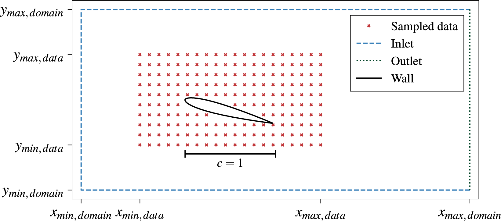
Like any numerical method, the domain and boundary conditions applied are key to obtaining physically meaningful results. As mentioned in Section 2.2, the purpose of the domain is to provide collocation points to evaluate the network across each loss component. A total of 180,000 training points (150,000 domain and 30,000 boundary points) were used to evaluate the physics and boundary losses, with 25,000 (20,000 domain and 5,000 boundary points) validation points used to evaluate these metrics and the network’s performance. All points were randomly generated using a Hammersley distribution, either through the domain or along its edge for boundary points. The number of collocation points was chosen to minimize training time and operate within the GPU’s memory constraints. In the work presented here, we will be investigating the application of PINNs to a stalled airfoil flow across a range of Reynolds numbers and data fidelities. Specifically, a NACA 0012 airfoil at an angle of attack,
$ \alpha $
 = 15° is selected at two Reynolds numbers of Re = 10,000 and 75,000. As shown by the schematic in Figure 1, the domain is constructed from an external box and an internal airfoil. Along the outer edges of the external box, we can prescribe the inlet and outlet conditions and treat the internal edge of the airfoil as a solid wall. This domain geometry is agnostic of any dataset or Reynolds number changes and will be fixed throughout all models. To ensure the PINN obeys the no-slip condition, we apply hard constraints along the surface of the airfoil. Soft constraints are applied to all other boundary conditions, including the data loss, to mitigate the increased computational cost and enable the flexibility of a PINN to handle noisy or erroneous data. Table 1 summarizes all PINN configurations’ applied boundary conditions.
Schematic of domain with representative data loss points within inner data “box” and boundaries for applied boundary conditions.
Boundary conditions applied to all PINN models, including type of constraint enforcement box

Table 1. Long description
The table consists of three columns: Boundary, Enforcement, and Constraints.
* Row 1: Inlet boundary has Soft enforcement. Constraints are U-bar equals 1, V-bar equals 0, and nu-tilde equals 4 nu-infinity.
* Row 2: Airfoil wall boundary has Hard enforcement. Constraints are U-bar equals V-bar equals f sub s comma x equals f sub s comma y equals nu-tilde equals 0.
* Row 3: Outlet boundary has no specified enforcement or constraints.
For all cases presented here, the domain remained fixed, with a length of 15c (−5c to 10c) and a height of 10c (−5c to 5c), where c is the chord length and is set to 1, with the airfoil leading edge located at the origin. This study considers four datasets in total, including two RANS simulations (R10 and R75), and two high-fidelity datasets from LES (L10) and PIV (P75), respectively. These will provide the reference data for the baseline models, as well as the transfer learning models, which will be pre-trained on RANS and then fine-tuned using either the PIV data or LES data as a clean validation case to eliminate experimental noise as a variable when training the PINN. With regard to the PINN configuration and training methodologies for these various models, full details are provided in Section 3. Specifically, Tables 3 and 4 describe the dimensions of the data box, the sub-sampling of the reference data, and the quantities used for training as part of the data loss, and those evaluated throughout the domain to validate the physical consistency of the PINN.
Table 2 details the base weights for the loss function described in Equation 2.9. The weights detailed here only apply to soft-enforced boundary conditions. As is common in the literature, two optimizers are utilized during training, Adam and L-BFGS, with different weights depending on the optimizer used throughout the different model training stages. For hard constrained boundary conditions, such as the airfoil wall, we assume
$ {\lambda}_B=1 $
 and the Lagrange multiplier is updated internally per collocation point on the boundary. The data provided, and quantities predicted, are scaled by the freestream velocity,
$ {\overline{U}}_{\infty } $
and the Lagrange multiplier is updated internally per collocation point on the boundary. The data provided, and quantities predicted, are scaled by the freestream velocity,
$ {\overline{U}}_{\infty } $
 , and the airfoil’s chord length, c. No additional scaling or normalization of the inputs or outputs was undertaken here, as seen in other areas of the literature.
Summary of loss function weights during Adam and L-BFGS optimization stages for all soft-enforced constraints
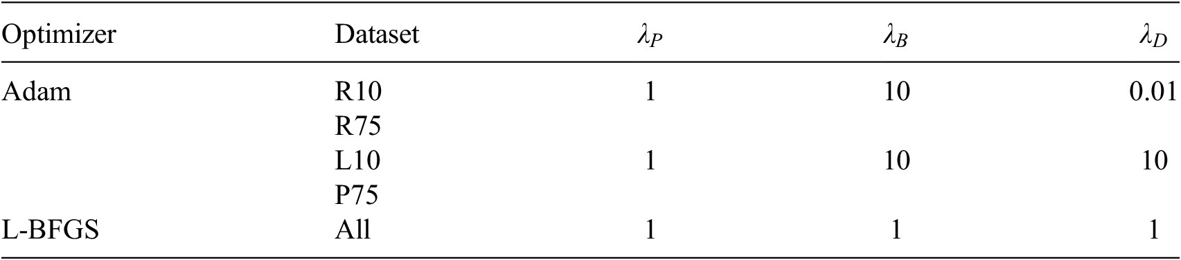
Table 2. Long description
The table consists of five columns: Optimizer, Dataset, lambda sub P, lambda sub B, and lambda sub D.
Under the Adam optimizer:
* For datasets R 10 and R 75, lambda sub P is 1, lambda sub B is 10, and lambda sub D is 0.01.
* For datasets L 10 and P 75, lambda sub P is 1, lambda sub B is 10, and lambda sub D is 10.
Under the L-B F G S optimizer:
* For all datasets, lambda sub P is 1, lambda sub B is 1, and lambda sub D is 1.
3. Transferring to high-fidelity data
To apply PINNs to higher Reynolds number problems efficiently using eddy viscosity models, we need to reconsider how we train these models. Section 3.1 summarizes the datasets used throughout this work for both the baseline and transfer learning models. Section 3.2 details a new methodology for incorporating the reference RANS eddy viscosity field within the data loss, which prevents the PINN from reaching a trivial solution for the eddy viscosity. Section 3.3 discusses how the RANS-trained baseline model can be fine-tuned through transfer learning to high-fidelity numerical or experimental datasets.
3.1. Reference datasets
To apply the proposed methodologies, we first need to fully define the reference data used for the generation of each model. For each PINN model and its accompanying reference data set, we can group each quantity into driving or driven quantities. Driving quantities are those that appear in the data loss, whereas driven quantities are those that do not feature in the data loss or are derivatives of the PINN’s predictions. It is important to make this distinction when analyzing the results, as we expect driving quantities to be predicted accurately, especially at the data location. However, driven quantities rely on the network to reconstruct them. By comparing the driven quantities for which we have data, we can have greater confidence in the physical interpretability of other quantities for which we do not have data.
For the two RANS datasets (R10 and R75), the driving quantities for the baseline models include
$ \overline{U},\overline{V} $
 and
$ \tilde{\nu} $
and
$ \tilde{\nu} $
 and the driven quantity for comparison is the pressure coefficient,
$ {C}_p $
and the driven quantity for comparison is the pressure coefficient,
$ {C}_p $
 , where

and
$ {q}_{\infty }=\frac{1}{2}\rho {\overline{U}}^2 $
 . For the PINN, due to the Helmholtz decomposition in Equation 2.2, the pressure coefficient is calculated by

When training with the RANS datasets, no sub-sampling is applied, where all 28,934 cells are used as data points with the driving quantities evaluated at these locations.
For the two high-fidelity datasets from LES and PIV (L10 and P75, respectively), the driving quantities will only include
$ \overline{U} $
 and
$ \overline{V} $
and
$ \overline{V} $
 . The driven quantities are the Reynolds shear stress,
$ \overline{u^{\prime }{v}^{\prime }} $
. The driven quantities are the Reynolds shear stress,
$ \overline{u^{\prime }{v}^{\prime }} $
 and
$ {C}_p $
and
$ {C}_p $
 . The reference data are provided in Figures 2 and 3 for comparison, both with the baseline models generated using these datasets, as well as for transfer learning. When comparing Figures 2 to 3, the necessity for experimental data over RANS becomes apparent. For this stalled airfoil case, RANS does not reliably capture the size of the recirculation bubble and the strength of the reverse flow region. Table 3 summarizes the quantities used in the data loss and sampling frequencies throughout the domain.
Reference fields for velocity, pressure coefficient,
$ {C}_p $
 , and eddy viscosity,
$ {\nu}_t $
, and eddy viscosity,
$ {\nu}_t $
 , fields for a NACA 0012 at
$ \alpha $
, fields for a NACA 0012 at
$ \alpha $
 = 15° from RANS at Re = 10,000 (left) and Re = 75,000 (right).
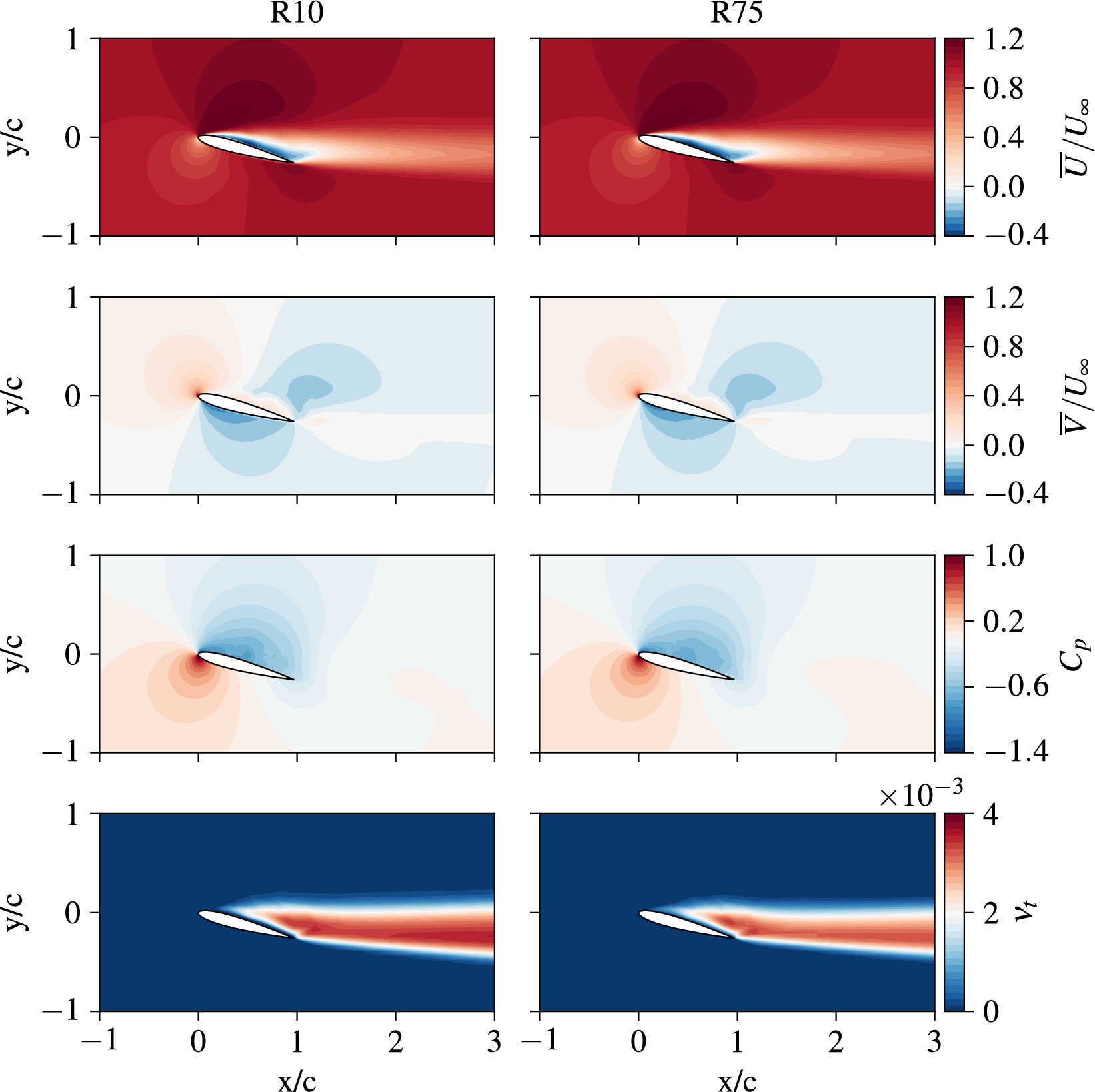
Figure 2. Long description
The grid consists of four rows and two columns. The x-axis for all panels ranges from negative 1 to 3 x all over c, and the y-axis ranges from negative 1 to 1 y all over c.
Row 1 shows the streamwise velocity U-bar all over U-infinity. The flow is characterized by a high-velocity red region surrounding the airfoil and a low-velocity blue wake trailing behind the trailing edge. The R 75 case shows a more defined and slightly thinner wake compared to R 10.
Row 2 shows the transverse velocity V-bar all over V-infinity. It features a dipole-like structure with positive velocity (red) above the leading edge and negative velocity (blue) below it.
Row 3 shows the pressure coefficient C sub p. A high-pressure red stagnation point is visible at the leading edge, with a low-pressure blue region on the upper suction surface. The R 75 case shows a more intense low-pressure zone.
Row 4 shows the eddy viscosity nu sub t. The field is mostly dark blue (zero) with a concentrated plume of red and white originating from the upper surface and trailing into the wake. The R 75 case shows a higher magnitude of eddy viscosity, indicated by a brighter red core in the wake, with a scale factor of 10 to the negative 3 power.
Color bars on the right of each row indicate the scale, ranging from blue (negative or low values) to red (positive or high values).
Reference fields for velocity, pressure coefficient,
$ {C}_p $
 , and Reynolds shear stress,
$ \overline{u^{\prime }{v}^{\prime }} $
, and Reynolds shear stress,
$ \overline{u^{\prime }{v}^{\prime }} $
 , fields for a NACA 0012 at
$ \alpha $
, fields for a NACA 0012 at
$ \alpha $
 = 15° from LES at Re = 10,000 (left) and PIV at Re = 75,000 (right). PIV
$ {C}_p $
= 15° from LES at Re = 10,000 (left) and PIV at Re = 75,000 (right). PIV
$ {C}_p $
 is computed using a Poisson solver and not directly measured.
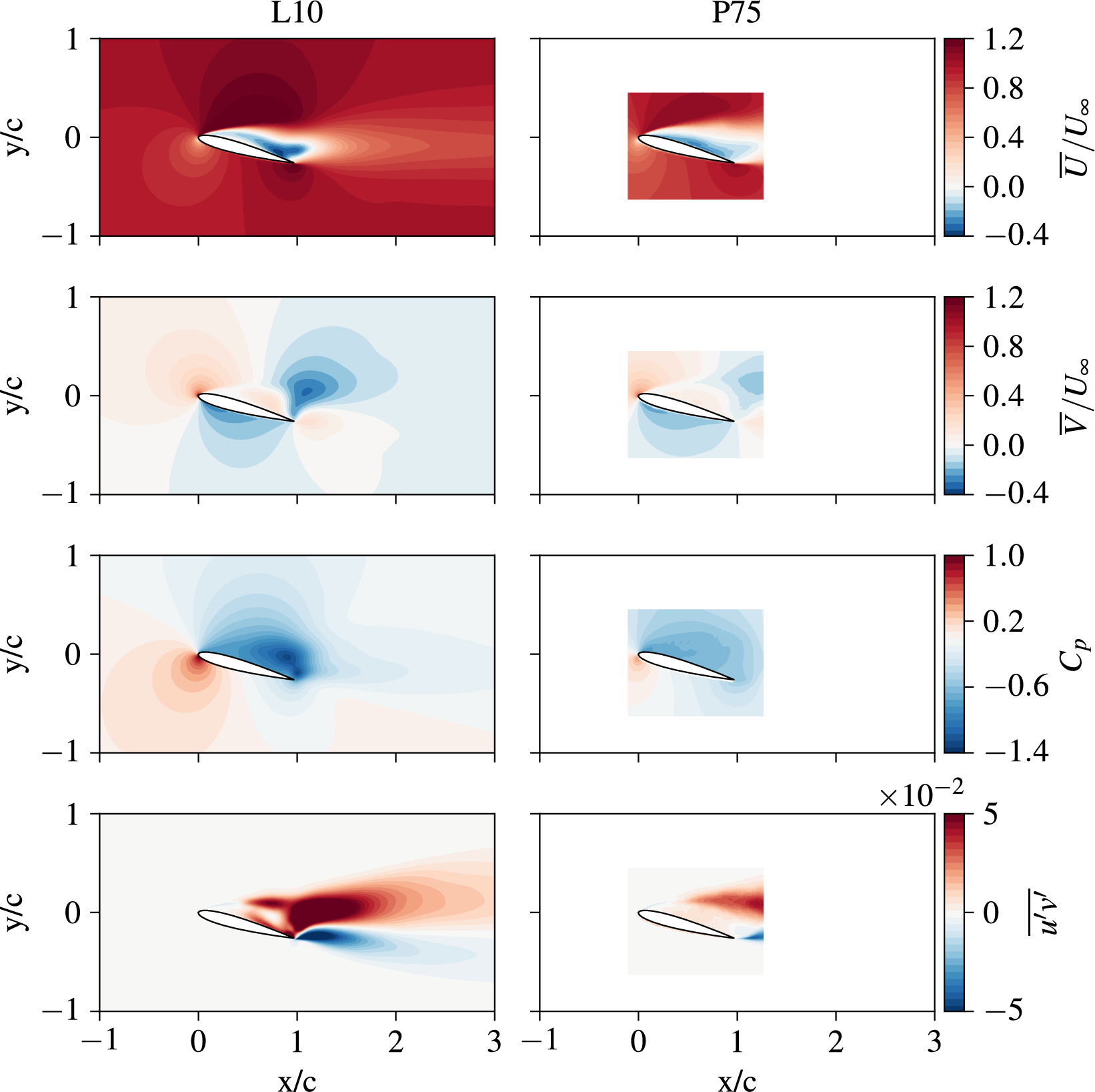
Figure 3. Long description
The grid uses x all over c as the horizontal axis from negative 1 to 3 and y all over c as the vertical axis from negative 1 to 1. Each row represents a different variable with a color scale on the right.
Row 1 shows horizontal velocity U bar all over U infinity. The L 10 panel shows a large wake of low velocity (blue) trailing from the airfoil trailing edge, while the P 75 panel shows a similar but more concentrated wake region.
Row 2 shows vertical velocity V bar all over V infinity. Both panels show a dipole-like structure with positive velocity (red) above the leading edge and negative velocity (blue) below and behind the airfoil.
Row 3 shows the pressure coefficient C sub p. A deep blue region of low pressure is visible on the upper surface of the airfoil in both L 10 and P 75, indicating suction, with a red high-pressure stagnation point at the leading edge.
Row 4 shows Reynolds shear stress u prime v prime overline. The L 10 panel displays a broad turbulent wake with high positive values (dark red) above the trailing edge and negative values (blue) below. The P 75 panel shows a similar but more spatially restricted shear layer.
The P 75 P I V data in the right column is presented within a smaller rectangular window compared to the full-field L 10 L E S data.
Summary of dimensions of the inner data box, driving quantities and their sampling frequency, and driven quantities for model validation of the baseline models
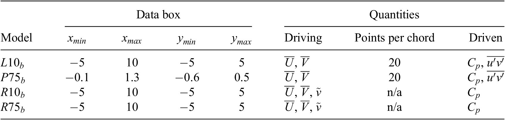
Table 3. Long description
The table is organized into eight columns. The first column lists the Model. The next four columns define the Data box dimensions: x sub min, x sub max, y sub min, and y sub max. The final three columns list Quantities: Driving, Points per chord, and Driven.
* Model L 10 sub b: Data box x from minus 5 to 10, y from minus 5 to 5. Driving quantities are U bar and V bar. Points per chord is 20. Driven quantities are C sub p and u prime v prime bar.
* Model P 75 sub b: Data box x from minus 0.1 to 1.3, y from minus 0.6 to 0.5. Driving quantities are U bar and V bar. Points per chord is 20. Driven quantities are C sub p and u prime v prime bar.
* Model R 10 sub b: Data box x from minus 5 to 10, y from minus 5 to 5. Driving quantities are U bar, V bar, and nu tilde. Points per chord is n forward slash a. Driven quantity is C sub p.
* Model R 75 sub b: Data box x from minus 5 to 10, y from minus 5 to 5. Driving quantities are U bar, V bar, and nu tilde. Points per chord is n forward slash a. Driven quantity is C sub p.
When utilizing these high-fidelity datasets, uniform sub-sampling of the data was undertaken to evaluate the PINNs’ performance with sparse measurements. In this process, there was no interpolation prior to sub-sampling to ensure that the PINN did not propagate any errors. The PIV data is from a set of experiments by Carter and Ganapathisubramani (Reference Carter and Ganapathisubramani2023). Whilst we sub-sampled the data at 20 points per chord, we dropped any data with clear post-processing errors or near the wall to improve training stability and prediction accuracy. This resulted in a total of 586 data points to evaluate both driving quantities when training with the PIV data. For the LES data, reducing the window size mimics a typical experimental field of view. This was also found to be beneficial for improving predictions in the wake by naturally focusing the optimizer to improve predictions in this region. Given the slightly larger data window, a total of 769 data points were used in training for evaluating the data loss.
Figure 4 shows the sub-sampled data, in red, against the full available data, in black, for both the LES and PIV datasets. For the LES data, the slight non-uniformity in the sampling is due to selecting the nearest neighbour to a uniform grid of points to avoid any potential interpolation errors.
Comparison of original reference data, in black, and sub-sampled data, in red, for the LES (left) and PIV (right) datasets, respectively.
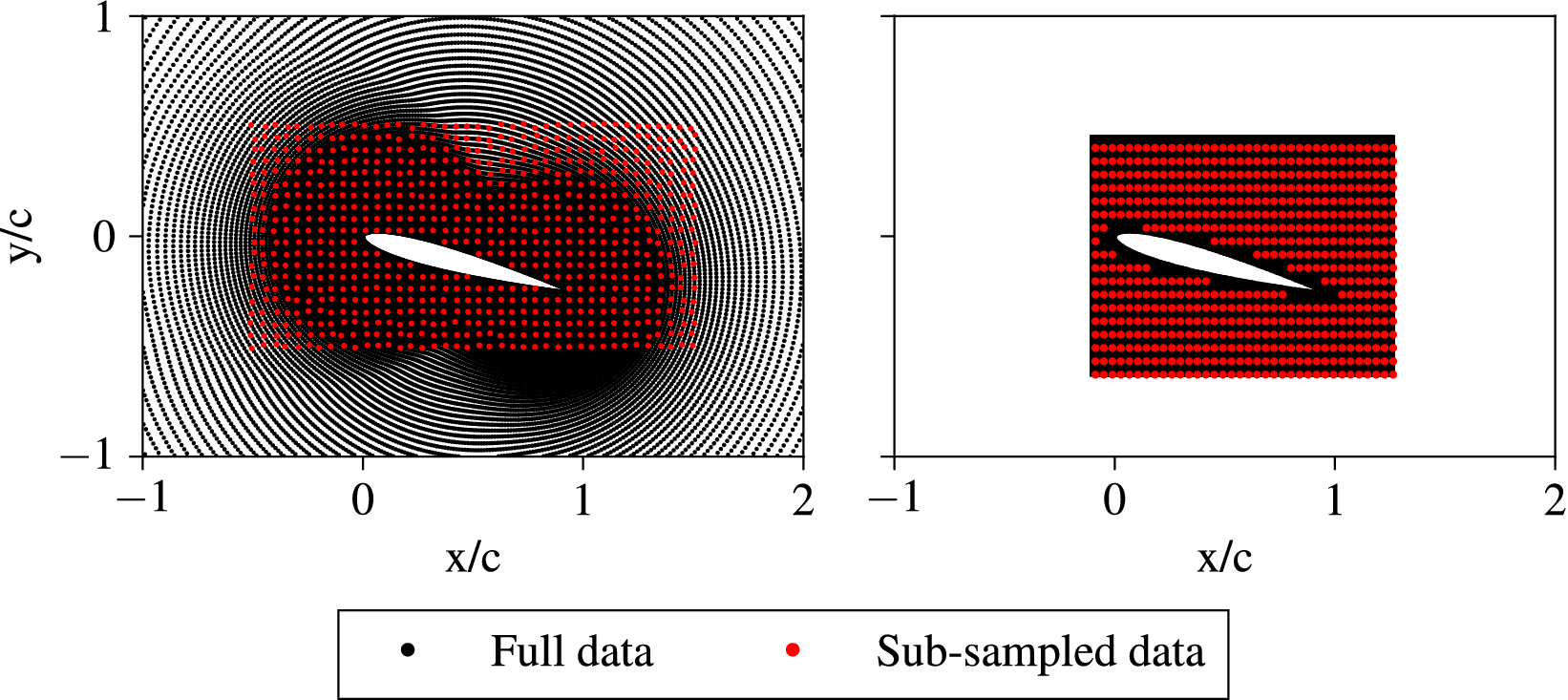
Figure 4. Long description
A two-panel scatter plot. Both panels share identical axes: the horizontal x forward slash c axis ranges from negative 1 to 2, and the vertical y forward slash c axis ranges from negative 1 to 1. At the center of each plot is a white, wing-shaped airfoil profile.
* The left panel, representing the L E S dataset, shows full data as black dots arranged in dense, concentric curvilinear patterns that follow the contours of the airfoil, filling the entire plot area. Overlaid on this is the sub-sampled data, shown as red dots forming a rectangular grid that concentrated around the airfoil from x forward slash c equals negative 0.5 to 1.5 and y forward slash c equals negative 0.5 to 0.5.
* The right panel, representing the P I V dataset, shows the full data as a solid black rectangular block. The sub-sampled data is represented by red dots arranged in a uniform, sparse grid that perfectly overlaps the black rectangular region, leaving the rest of the plot area white and empty.
A legend at the bottom indicates that black dots represent Full data and red dots represent Sub-sampled data.
3.2. Baseline training
In much of the recent literature surrounding PINNs, the training process of the neural network is a combination of stochastic gradient descent-based optimization (e.g. Adam) followed by a quasi-Newton method (e.g. L-BFGS) until convergence (Raissi et al., Reference Raissi, Perdikaris and Karniadakis2019; Sliwinski and Rigas, Reference Sliwinski and Rigas2023). This process has been largely effective for various fluid-based problems but presents issues with training stability for PINNs using a turbulence model (Patel et al., Reference Patel, Mons, Marquet and Rigas2024). In this work, we propose that a negative feedback loop drives the issue, where erroneous mean velocity gradients in the initial predictions produce incorrect eddy viscosity production, which, in turn, causes further issues with the predicted velocity field later in the training process.
To overcome this issue, we propose splitting the training procedure into two distinct sections. First, the PINN undergoes training using the RANS-F equation set with just an Adam optimizer to stabilize the velocity field to a more physical regime. Following this, a second Adam optimization step with the RANS-SA equations is taken at a reduced learning rate to mitigate any significant changes in the velocity field. The training procedure concludes using an L-BFGS optimizer until convergence. Algorithm 1 provides the full details, and this procedure will apply to all baseline models in Section 4.
Algorithm 1. Baseline model—network training process with adaptive learning rate.
1 Input: Network parameters
$ {\theta}_0=\left(\mathbf{W},\mathbf{b}\right) $
 , loss function
$ \mathrm{\mathcal{L}}\left(\theta \right) $
, loss function
$ \mathrm{\mathcal{L}}\left(\theta \right) $
 .
.
2 Set equation to RANS-F
3 for
$ t\leftarrow 1 $
 to
$ \mathrm{100,000} $
to
$ \mathrm{100,000} $
 do
do
4 Optimize
$ {\theta}_t\leftarrow \mathtt{Adam}\left(\mathrm{\mathcal{L}}\left({\theta}_{t-1}\right),\gamma \right) $
 .
.
5 if plateau detected over
$ \mathrm{5,000} $
 steps then
6
$ \gamma \leftarrow \gamma \cdot {\gamma}_{\mathrm{plateau}} $

7 end
8 end
9 Set equation to RANS-SA.
10
$ \gamma \leftarrow {10}^{-4} $

11 for
$ t\leftarrow 1 $
 to
$ \mathrm{50,000} $
to
$ \mathrm{50,000} $
 do
do
12 Optimize
$ {\theta}_t\leftarrow \mathtt{Adam}\left(\mathrm{\mathcal{L}}\left({\theta}_{t-1}\right),\gamma \right) $
 .
.
13 if plateau detected over
$ \mathrm{5,000} $
 steps then
14
$ \gamma \leftarrow \gamma \cdot {\gamma}_{\mathrm{plateau}} $

15 end
16 end
17
$ \gamma \leftarrow 1 $

18 for
$ t\leftarrow 1 $
 to convergence do
19 Optimize
$ {\theta}_t\leftarrow \mathtt{L}\hbox{-} \mathtt{BFGS}\left(\mathrm{\mathcal{L}}\left({\theta}_{t-1}\right),\gamma \right) $

20 end
21 Output: Final network parameters
$ {\theta}_t $
 .
.
22 Defaults:
$ \gamma ={10}^{-3},{\gamma}_{\mathrm{plateau}}=0.5,{\theta}_0=\left(\mathbf{W}\sim U\left(-\sqrt{3}/2,\sqrt{3}/2\right),\mathbf{b}\leftarrow 0\right) $
 .
.
Alongside giving us a reference of the performance of a PINN with different datasets of the same problem, the baseline models provide a starting point for applying transfer learning. Table 3 provides a summary of the four models that will be trained using Algorithm 1, which will act as a source of comparison to the transfer learning cases (
$ L{10}_b $
 &
$ P{75}_b $
&
$ P{75}_b $
 ) and as an initialization for the transfer learning models (
$ R{10}_b $
) and as an initialization for the transfer learning models (
$ R{10}_b $
 &
$ R{75}_b $
&
$ R{75}_b $
 ).
).
3.3. Transfer learning
One of the shortcomings of PINNs is their inherent embedding of the flow configuration in the network, limiting direct application to a new problem, such as a change in geometry, without additional steps or modification to the network architecture. However, for a sufficiently similar flow problem, it is reasonable to assume that the resulting solution, or network parameters for a PINN, would be comparable. Therefore, this limitation can also be seen as a feature, as many problems rely on a fixed geometry but vary parameters such as the Reynolds number. One approach to leverage this feature is through transfer learning.
Transfer learning is the process in neural networks of fine-tuning a pre-trained model on a new dataset to enhance its predictive capabilities for a specific task related to that dataset (Weiss et al., Reference Weiss, Khoshgoftaar and Wang2016). This technique commonly appears in fields such as large language models (LLMs) and computer vision tasks, where training one of these models from scratch would be prohibitively expensive or yield worse overall results. In the context of PINNs, we can take a pre-existing model and re-train the model at a reduced learning rate with a new dataset, replacing the existing data loss term within the loss function.
Algorithm 2: Transfer learning training process—RANS-SA only.
1 Input: Network parameters
$ {\theta}_0 $
 , loss function
$ \mathrm{\mathcal{L}}\left(\theta \right) $
, loss function
$ \mathrm{\mathcal{L}}\left(\theta \right) $
 .
.
2 for
$ t\leftarrow 1 $
 to
$ \mathrm{10,000} $
to
$ \mathrm{10,000} $
 do
do
3 Optimize
$ {\theta}_t\leftarrow \mathtt{Adam}\left(\mathrm{\mathcal{L}}\left({\theta}_{t-1}\right),\gamma \right) $

4 end
5
$ \gamma \leftarrow 1 $

6 for
$ t\leftarrow 1 $
 to convergence do
7 Optimize
$ {\theta}_t\leftarrow \mathtt{L}\hbox{-} \mathtt{BFGS}\left(\mathrm{\mathcal{L}}\left({\theta}_{t-1}\right),\gamma \right) $

8 end
9 Output: Final network parameters
$ {\theta}_t $
 .
.
10 Defaults:
$ \gamma ={10}^{-4},{\theta}_0={\left(\mathbf{W},\mathbf{b}\right)}_{\mathrm{baseline}} $

There are many permutations of transfer learning available with varying levels of freedom given to the new network to update its parameters through the number of iterations, learning rate, or available parameters to update (otherwise referred to as frozen/unfrozen layers) (Torrey and Shavlik, Reference Torrey and Shavlik2010). As outlined in Algorithm 2, the process for the work presented here is quite simplistic, reducing only the number of iterations and learning rate. This decision helps reduce the parameter space to search when generating these models, but further optimization of this process through more complex procedures may be possible. For all models using transfer learning through Section 4, Algorithm 2 has been used to train the new model.
This method proposes fine-tuning with the experimental data from a baseline model of a matching geometry. To investigate this, as shown in Figure 5, we generate baseline models from a low-fidelity RANS dataset for two Reynolds numbers and then apply transfer learning to either of the two high-fidelity datasets. For the four models in Table 4, we consider matching Reynolds numbers and the feasibility of scaling up or down from the baseline model Reynolds numbers. This study omits the application of transfer learning between similar fidelity data, as we are primarily interested in transitioning from RANS to experimental data, as denoted by the dashed arrows in Figure 5. Table 4 also summarizes the sampling frequency and quantities provided for training and validation, respectively.
Flowchart of possible transfer learning options with solid arrows indicating those investigated (with associated model name labeled—subscript “
$ b $
 ” indicating baseline model) and dashed arrows indicating those disregarded.
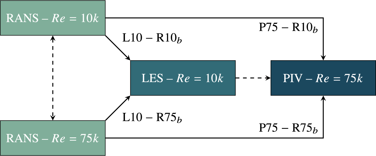
Figure 5. Long description
The flowchart consists of four rectangular nodes connected by solid and dashed arrows.
On the far left, there are two green source nodes arranged vertically.
* The top node is labeled R A N S minus R e equals 10 k.
* The bottom node is labeled R A N S minus R e equals 75 k.
* A vertical dashed double-headed arrow connects these two nodes, indicating a disregarded relationship.
In the center is a teal node labeled L E S minus R e equals 10 k.
* A solid arrow points from R A N S minus R e equals 10 k to this center node, labeled L 10 minus R 10 sub b.
* A solid arrow points from R A N S minus R e equals 75 k to this center node, labeled L 10 minus R 75 sub b.
On the far right is a dark blue node labeled P I V minus R e equals 75 k.
* A solid arrow originates from the top-left R A N S node and points to the top of the P I V node, labeled P 75 minus R 10 sub b.
* A solid arrow originates from the bottom-left R A N S node and points to the bottom of the P I V node, labeled P 75 minus R 75 sub b.
* A horizontal dashed arrow points from the center L E S node to the P I V node, indicating a disregarded path.
Summary of dimensions of the inner data box, driving quantities and their sampling frequency, and driven quantities for model validation of the transfer learning cases
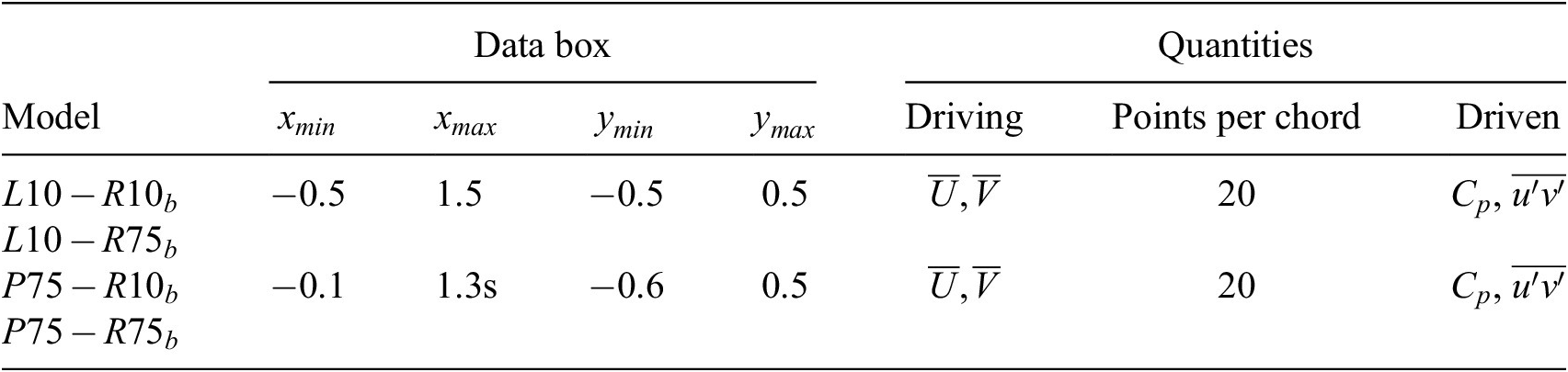
Table 4. Long description
The table is divided into three main sections: Model, Data box, and Quantities.
* The Data box section includes four columns: x sub min, x sub max, y sub min, and y sub max.
* The Quantities section includes three columns: Driving, Points per chord, and Driven.
Row 1 and 2: Models L 10 minus R 10 sub b and L 10 minus R 75 sub b.
* Data box: x sub min is negative 0.5, x sub max is 1.5, y sub min is negative 0.5, y sub max is 0.5.
* Quantities: Driving is U-bar, V-bar; Points per chord is 20; Driven is C sub p, u-prime v-prime-bar.
Row 3 and 4: Models P 75 minus R 10 sub b and P 75 minus R 75 sub b.
* Data box: x sub min is negative 0.1, x sub max is 1.3s, y sub min is negative 0.6, y sub max is 0.5.
* Quantities: Driving is U-bar, V-bar; Points per chord is 20; Driven is C sub p, u-prime v-prime-bar.
One advantage of transfer learning is the subsequent reduction in training time after the first model. For the baseline models trained using Algorithm 1, the total training time is approximately 10 hours using an NVIDIA A100 GPU, whereas those using the transfer learning process only require one hour on equivalent hardware. The full details of training time in terms of iterations and wall time are summarized in Table 5. This cost-saving highlights one of the other potential advantages, particularly when applying large datasets to PINNs.
Summary of PINN training algorithms and computational time box

Table 5. Long description
The table consists of four columns and two data rows.
Column headers from left to right are:
1. Algorithm.
2. Adam iterations.
3. L-B F G S iterations.
4. Wall time in hours.
Data rows:
Row 1: Algorithm 1. Baseline. Adam iterations: 150,000. L-B F G S iterations: 50,000 or convergence. Wall time: 10.
Row 2: Algorithm 2. Transfer learning. Adam iterations: 10,000. L-B F G S iterations: 50,000 or convergence. Wall time: 1 plus 10 for baseline.
4. Results
The results section follows the order of the models defined in Section 3. Section 4.1 outlines the difficulties of training PINNs directly with experimental data and how these challenges are consistent when using LES data. Section 4.2 applies the same baseline training methodology to the RANS datasets for models
$ R{10}_b $
 and
$ R{75}_b $
and
$ R{75}_b $
 . Section 4.3 presents the transfer learning, initially applied to the LES dataset, as a validation case of the proposed methodology, and the importance of hard constraints. Section 4.4 then applies the transfer learning method to the PIV data. Section 4.5 summarizes the findings from the results section and presents the results for the transfer learning models where the baseline Reynolds number is different from the high-fidelity dataset.
4.1. PINNs with high-fidelity data
To highlight some of the issues with working from high-fidelity data directly with PINNs, we first created two PINN models without using transfer learning. These models,
$ L{10}_b $
 and
$ P{75}_b $
and
$ P{75}_b $
 , follow the creation procedure of the baseline model process outlined in Algorithm 1 and the parameters outlined through Section 3. For all comparisons, we will consider their relative difference where the error,
$ \unicode{x025B} $
, follow the creation procedure of the baseline model process outlined in Algorithm 1 and the parameters outlined through Section 3. For all comparisons, we will consider their relative difference where the error,
$ \unicode{x025B} $
 , is given as,

for the driving variables. For the driven variables, we will only consider the structures and magnitudes of the predicted quantities against the reference values.
For the LES baseline PINN, Figure 6 shows the prediction of the driving variables (
$ \overline{U}\&\overline{V} $
 ) and their error,
$ \unicode{x025B} $
) and their error,
$ \unicode{x025B} $
 . As the velocity components are in the data loss for the PINN, it is expected to get a good agreement between the reference fields and the predictions. For the bulk of the wake, there is a small residual error, but the large structures, such as the recirculation region, are closely matched. The largest error is near the airfoil surface on the pressure side of the wing. Whilst the data is sub-sampled, data points are provided up to the surface of the airfoil with no additional masking of the near-wall region. With sparse data, it is reasonable to assume that the PINN is unable to reconstruct the correct velocity gradients, and the sensitivity to those gradients has resulted in the PINN optimizing towards a non-physical solution in this region of the domain. Therefore, to improve on this, we would likely need more data close to or on the wall.
PINN predicted fields from model L
$ {10}_b $
 of the driving quantities for each velocity component,
$ \overline{U}\&\overline{V} $
of the driving quantities for each velocity component,
$ \overline{U}\&\overline{V} $
 , and their respective errors to reference the L10 dataset. For
$ \overline{U} $
, and their respective errors to reference the L10 dataset. For
$ \overline{U} $
 , the dashed line indicates the edge of the recirculation region from the experimental data.
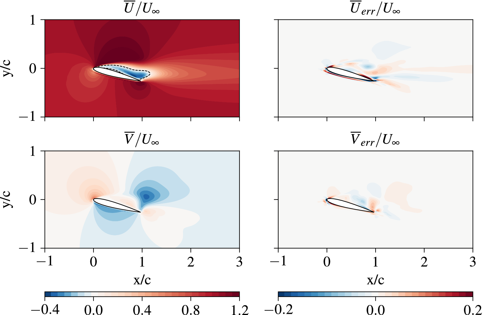
Figure 6. Long description
The multi-panel figure consists of two rows and two columns of contour plots. All plots show an airfoil centered near the origin. The horizontal axis represents x all over c ranging from negative 1 to 3. The vertical axis represents y all over c ranging from negative 1 to 1.
* Top-Left Panel: Displays U-bar all over U-infinity. It shows a high-velocity red region above and below the airfoil. A dashed line on the upper surface of the airfoil indicates the recirculation region boundary. The color scale at the bottom left ranges from negative 0.4 blue to 1.2 dark red.
* Top-Right Panel: Displays U-bar sub err all over U-infinity. The field is mostly neutral white with small patches of blue and red concentrated near the airfoil surfaces and wake. The color scale at the bottom right ranges from negative 0.2 blue to 0.2 dark red.
* Bottom-Left Panel: Displays V-bar all over U-infinity. It shows a dipole-like structure with a light red region above the leading edge and a blue region above the trailing edge. It uses the same negative 0.4 to 1.2 scale as the top-left panel.
* Bottom-Right Panel: Displays V-bar sub err all over U-infinity. Similar to the top-right panel, the errors are localized around the airfoil geometry and trailing edge, using the negative 0.2 to 0.2 scale.
Figure 7 highlights this non-physical solution near the airfoil’s lower surface and how it propagates to neighboring regions of the domain. While away from the surface of the airfoil, the pressure contours have a good agreement with the reference data; the main issue is focused towards the leading edge. On closer inspection, it appears the surface of the airfoil has been offset slightly upstream, resulting in an unphysical prediction of the pressure. The conclusion is that the PINN tends toward an unphysical solution when there is negative feedback between the velocity gradients and the equations, as the pressure is only constrained by the physics loss here. A similar conclusion can also be drawn when looking at the Reynolds shear stress in Figure 7, where the bulk of the prediction away from the airfoil has a reasonable agreement but struggles close to the airfoil, particularly on the airfoil’s pressure side. This suggests that with more data around the airfoil, we could get much better results as the physics are largely matched elsewhere in the flow.
PINN predicted fields from model L
$ {10}_b $
 of the driven quantities, including the pressure coefficient,
$ {C}_p $
of the driven quantities, including the pressure coefficient,
$ {C}_p $
 , and Reynolds shear stress,
$ \overline{u^{\prime }{v}^{\prime }} $
, and Reynolds shear stress,
$ \overline{u^{\prime }{v}^{\prime }} $
 .
.
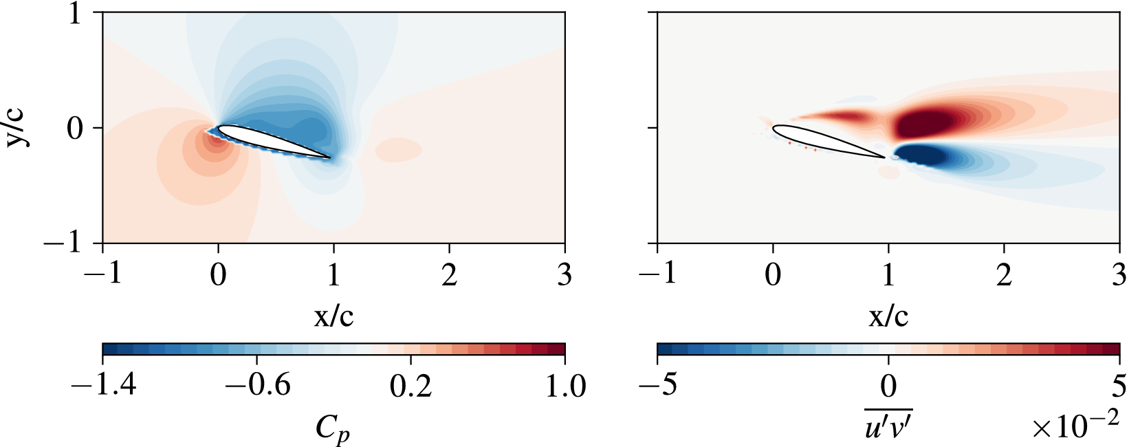
Figure 7. Long description
The figure consists of two side-by-side panels. Both panels share a horizontal x all over c axis ranging from negative 1 to 3 and a vertical y all over c axis ranging from negative 1 to 1. An airfoil is centered at the origin in both plots.
Left Panel: Displays the pressure coefficient C sub p. A color scale at the bottom ranges from negative 1.4 in dark blue to 1.0 in dark red. The plot shows a large blue region of negative pressure above the airfoil and a red region of positive pressure at the leading edge and below the airfoil.
Right Panel: Displays the Reynolds shear stress u prime v prime overline. A color scale at the bottom ranges from negative 5 times 10 to the negative 2 power in dark blue to 5 times 10 to the negative 2 power in dark red. The plot shows a concentrated red wake region extending from the upper surface of the airfoil and a blue wake region extending from the lower trailing edge, indicating turbulent stress distribution.
For the PIV baseline PINN, in Figure 8, we can see that the presence of a turbulence model allows us to accurately predict the recirculation region with good agreement with the reference data from Figure 3. Outside of the PIV window, in the far wake region, the contours show that the turbulence model is correctly applying the additional dissipation for the velocity field to recover physically. However, we can see where the PINN struggles using this baseline methodology when considering the error plots. For example, with PIV, resolving the near wall can be challenging due to the presence of reflections on the surface from the laser. Therefore, we could attribute errors in that region to poor reference data rather than the PINN failing to model the physics correctly. In this case, the errors are in three distinct regions: the stagnation point, the near wall, and the shear layer.
PINN predicted fields from model P
$ {75}_b $
 of the driving quantities for each velocity component,
$ \overline{U}\&\overline{V} $
of the driving quantities for each velocity component,
$ \overline{U}\&\overline{V} $
 , and their respective errors to reference P75 dataset. For
$ \overline{U} $
, and their respective errors to reference P75 dataset. For
$ \overline{U} $
 , the dashed line indicates the edge of the recirculation region from the experimental data.
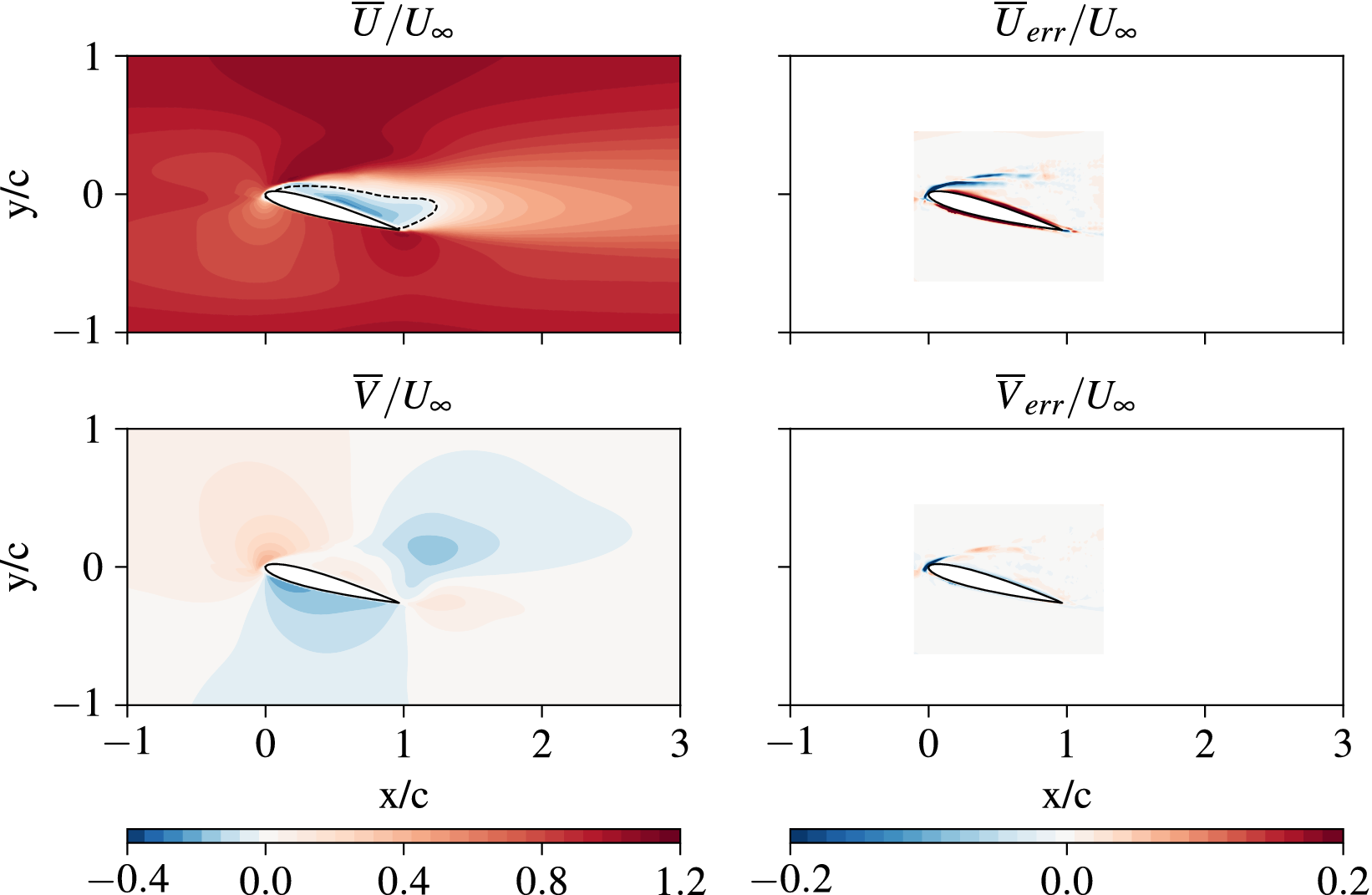
Figure 8. Long description
The figure consists of a two by two grid of contour plots. All plots share an x over c axis from negative 1 to 3 and a y over c axis from negative 1 to 1. An airfoil is centered at the origin.
Top-left panel: Displays U-bar over U-infinity. It shows a red-toned velocity field with a dashed line indicating a recirculation region behind the airfoil. The flow is highest in dark red regions above and below the airfoil.
Bottom-left panel: Displays V-bar over U-infinity. It shows a dipole-like structure with light red positive values above the leading edge and light blue negative values below the leading edge.
Top-right panel: Displays U-bar sub err over U-infinity. It shows the error distribution for the horizontal velocity component, with concentrated blue and red streaks near the airfoil surface and wake.
Bottom-right panel: Displays V-bar sub err over U-infinity. It shows the error distribution for the vertical velocity component, with minimal visible error except for small blue and red spots at the leading and trailing edges.
Two color bars are located at the bottom. The left color bar for the velocity fields ranges from negative 0.4 in blue to 1.2 in dark red. The right color bar for the error fields ranges from negative 0.2 in blue to 0.2 in dark red, with white representing zero error.
Starting with the shear layer, we see a large underprediction in the velocity, which appears to be a secondary recirculation region. This observation is unphysical and can be attributed to an issue with the PINN when working with a complex flow with erroneous data points. For the near-wall predictions, the error is likely a PIV issue rather than the PINN, given the consistency in the wall-normal distance of the error along the chord. However, this argument is not applicable to the stagnation point. Relative to the rest of the domain, the stagnation point is a small region with a large amount of physics to capture, which presents an issue for the PINN. With limited data points in this region, the PINN can only rely on the physics loss to model the velocity gradients here. Therefore, as seen by the concentration of error and discontinuous contours, the PINN cannot accurately model the stagnation point.
The driven variables in Figure 9 reinforce the observations of this model’s predictions. From the pressure, we can see that the maximum
$ {C}_p $
 is not on the airfoil surface. Additionally, the lack of a stagnation point is likely affecting the magnitude of the pressure along the suction side with a reduced acceleration over the leading edge. The comparison of the second-order statistics in the form of the Reynolds shear stress showcases the overfitting present in this PINN model. Critically, when discussing overfitting, there are two aspects to consider: overfitting to the data, where the driving quantity errors are high in locations where data is not provided (as we are only giving a coarse, sub-sampled dataset), and secondly, overfitting to the equations, where the driven, or validation, quantities are not physical. In this case, the former aligns with the aforementioned observations and results depicted in Figure 8. For the latter, this type of overfitting is shown by the Reynolds stresses in Figure 9, where the general structure bears similarities to the PIV data, but its presence before the leading edge and discontinuities in other regions of the flow indicate a lack of physical meaning from the turbulence model and forcing. As our predicted Reynolds stresses are computed using the eddy viscosity and mean velocity gradients, from Equation 2.4, the error seen in Figure 9 is directly a consequence of the eddy viscosity having large discontinuities and otherwise unphysical features throughout the domain. From this baseline case, it is clear that an alternative approach is necessary for effectively integrating experimental data with PINNs.
PINN predicted fields from model P
$ {75}_b $
 of the driven quantities, including the pressure coefficient,
$ {C}_p $
of the driven quantities, including the pressure coefficient,
$ {C}_p $
 , and Reynolds shear stress,
$ \overline{u^{\prime }{v}^{\prime }} $
, and Reynolds shear stress,
$ \overline{u^{\prime }{v}^{\prime }} $
 .
.
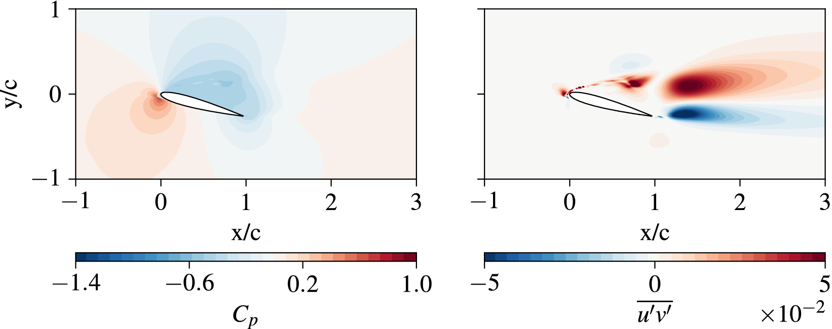
Figure 9. Long description
A two-panel visualization of fluid dynamics. Both panels use x all over c as the horizontal axis ranging from negative 1 to 3 and y all over c as the vertical axis ranging from negative 1 to 1. An airfoil is centered at the origin.
Left panel: Displays the pressure coefficient C sub p. A color scale at the bottom ranges from negative 1.4 in dark blue to 1.0 in dark red. The plot shows a high-pressure red region at the leading edge stagnation point and a low-pressure blue region over the upper suction surface of the airfoil.
Right panel: Displays the Reynolds shear stress u prime v prime overline. A color scale at the bottom ranges from negative 5 to 5 times 10 to the negative 2 power. The plot shows a wake trailing from the airfoil with a distinct dipole structure. A large red plume of positive shear stress extends above the wake centerline and a corresponding blue plume of negative shear stress extends below it, both originating near the trailing edge and expanding as they move downstream to the right.
4.2. Baseline models
To implement transfer learning with high-fidelity data, we first need to create a baseline model. Here, we intend to create a model that captures some of the fundamental features in the flow, such as the position of the stagnation point and the no-slip wall. The fine-tuning training procedure can then modify approximated features, such as the recirculation region, to match the high-fidelity dataset. By building the baseline model from an RANS dataset, we can directly use the eddy viscosity field from the CFD data as a data loss to avoid a trivial solution. The key assumption here is that between the different data fidelities, the similarity of the flow features should result in similar structures of turbulence production, and the PINN will only need to slightly modify the predicted eddy viscosity.
Figure 10 shows the predictions of these RANS baseline models. Across the baseline models, we see a good agreement between the predictions and the reference data outlined in Figure 2, with the predicted fields capturing the key structures across all quantities, including those where data was not provided. Unlike the PIV baseline, the RANS baseline models can capture fundamental features such as the stagnation point. The presence of increased near-wall data from the refinement in the CFD mesh likely enables this in the RANS models. This level of resolution and proximity to the wall would be very challenging to acquire through methods such as PIV. Therefore, when utilizing these baseline models for transfer learning, the objective is to provide reasonable estimates in regions of the flow for which we would not have data.
PINN predictions for
$ R{10}_b $
 and
$ R{75}_b $
and
$ R{75}_b $
 models for the error in each velocity component,
$ \overline{U}\&\overline{V} $
models for the error in each velocity component,
$ \overline{U}\&\overline{V} $
 , the pressure coefficient,
$ {C}_p $
, the pressure coefficient,
$ {C}_p $
 , and eddy viscosity,
$ {\nu}_t $
, and eddy viscosity,
$ {\nu}_t $
 .
.

Figure 10. Long description
The grid uses x forward slash c on the horizontal axis ranging from negative 1 to 3 and y forward slash c on the vertical axis ranging from negative 1 to 1. An airfoil shape is centered at the origin in every plot.
* Row 1 shows U bar err forward slash U infinity. Both models show low error (white) in the far field with small pockets of positive (red) and negative (blue) error concentrated along the upper surface and wake of the airfoil.
* Row 2 shows V bar err forward slash V infinity. Errors are localized near the leading and trailing edges, with R 75 sub b showing slightly more fragmented error patterns compared to R 10 sub b.
* Row 3 shows the pressure coefficient C sub p. Both models display a smooth gradient with a high-pressure region (red) at the leading edge and a low-pressure region (blue) over the upper surface. The distributions are nearly identical between the two models.
* Row 4 shows eddy viscosity nu sub t with a scale factor of 10 to the negative 3 power. R 10 sub b shows a broad, somewhat noisy distribution of eddy viscosity in the wake. In contrast, R 75 sub b shows a much smoother, more concentrated plume of high eddy viscosity (red) trailing directly behind the airfoil, indicating a more refined prediction.
One of the fundamental challenges when implementing a turbulence model is avoiding a trivial solution, given the nature of the transport equation, Equation 2.5, and the typical magnitudes of
$ {\nu}_t $
 . By providing this quantity in the data loss, we can reduce the likelihood of this occurring, and whilst the accuracy is much closer for the R
$ {75}_b $
. By providing this quantity in the data loss, we can reduce the likelihood of this occurring, and whilst the accuracy is much closer for the R
$ {75}_b $
 model, as shown in Figure 10, some of the unphysical features in the R
$ {10}_b $
model, as shown in Figure 10, some of the unphysical features in the R
$ {10}_b $
 model highlights that the model is not overfitting to the data. Furthermore, the similarities in both predicted pressures of models R
$ {10}_b $
model highlights that the model is not overfitting to the data. Furthermore, the similarities in both predicted pressures of models R
$ {10}_b $
 and R
$ {75}_b $
and R
$ {75}_b $
 reinforce the idea that the PINN trained using this methodology does not overfit and highlight the non-uniqueness in the solutions to the transport equation.
4.3. PINNs with transfer learning to LES data
One possibility when working with experimental data is that the dataset contains too much noise or otherwise erroneous data points that make applying it to PINNs unfeasible, as the underlying physics of the data may be too far from the truth. For example, the measured velocity field may not obey 2D continuity, which would be true for a stalled airfoil flow that would have some spanwise component. The source of this error could be a combination of experimental uncertainties or missing velocity components in the case of planar PIV. Therefore, to isolate this problem when testing transfer learning, we initially investigated this using an LES dataset. Appendix A contains further information on generating and validating this dataset. For the following sections, all models follow Algorithm 2 and use the parameters outlined in Section 3.
4.3.1.
$ L10-R{10}_b $


In this case, we consider the application of transfer learning between datasets of equivalent Reynolds numbers of Re = 10,000. For the PINN, this should be the most straightforward case with both clean data and a lower Reynolds number. From Figure 11, we can see that the PINN has been able to modify the velocity field, particularly around the recirculation region. For the streamwise component, the PINN has modified the original recirculation bubble away from the airfoil surface, allowing it to expand in size. The dashed streamline, denoting the reference zero velocity contour, clearly illustrates this ability to capture the new profile. While we cannot directly compare to the LES baseline (L
$ {10}_b $
 ) predictions, the problematic features in that model have either been fully mitigated or reduced in magnitude. This model shows that the error focuses primarily on the leading edge and stagnation point. However, unlike the LES baseline model, this error does not propagate along the airfoil in the near-wall region.
PINN predicted fields from model
$ L10-R{10}_b $
 of the driving quantities for each velocity component,
$ \overline{U}\&\overline{V} $
of the driving quantities for each velocity component,
$ \overline{U}\&\overline{V} $
 , and their respective errors to reference L10 dataset. For
$ \overline{U} $
, and their respective errors to reference L10 dataset. For
$ \overline{U} $
 , the dashed line indicates the edge of the recirculation region from the LES data.
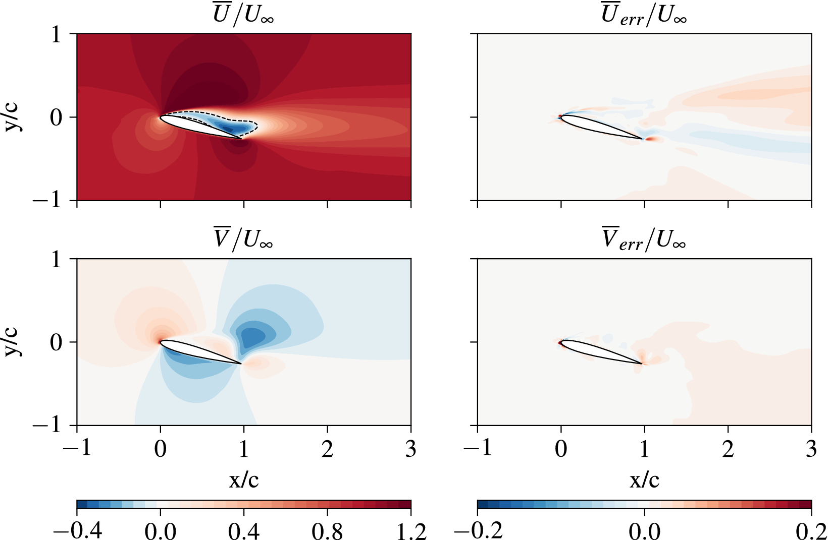
Figure 11. Long description
A four-panel grid of contour plots. Each plot shares an x-axis labeled x forward slash c ranging from negative 1 to 3 and a y-axis labeled y forward slash c ranging from negative 1 to 1. A white airfoil shape is centered at the origin in every panel.
* Top-left panel, U-bar over U-infinity. Shows a red-dominant field indicating high velocity. A dark blue region with a dashed black outline appears directly above the airfoil trailing edge, representing the recirculation zone.
* Top-right panel, U-bar sub err over U-infinity. Shows a mostly white field indicating low error, with faint red and blue streaks trailing behind the airfoil.
* Bottom-left panel, V-bar over U-infinity. Displays a dipole-like pattern with light blue and light red lobes around the airfoil, indicating vertical velocity components.
* Bottom-right panel, V-bar sub err over U-infinity. Shows a nearly uniform white field with very minor orange tinting in the wake region.
Two color bars are at the bottom. The left bar for velocity fields ranges from negative 0.4 blue to 1.2 dark red. The right bar for error fields ranges from negative 0.2 blue to 0.2 dark red.
We can also examine the driven variables in Figure 12 to verify these results and ensure the model does not overfit the new data. For the pressure, we can see that the PINN has recreated some of the defining features, such as the low-pressure region over the trailing edge. However, the limits of the pressure are under-predicted for both the suction side and the stagnation point. Notably, the stagnation point is slightly displaced from the airfoil surface, as indicated by the concentration of error near the leading edge in Figure 11. As with the LES baseline, this inability to capture the stagnation points likely generates lower pressures downstream.
PINN predicted fields from model
$ L10-R{10}_b $
 of the driven quantities, including the pressure coefficient,
$ {C}_p $
of the driven quantities, including the pressure coefficient,
$ {C}_p $
 , and Reynolds shear stress,
$ \overline{u^{\prime }{v}^{\prime }} $
, and Reynolds shear stress,
$ \overline{u^{\prime }{v}^{\prime }} $
 .
.
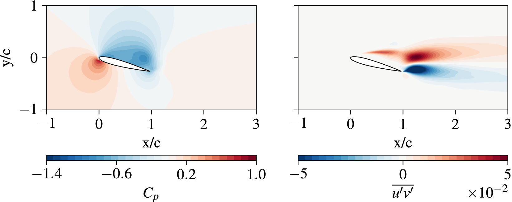
Figure 12. Long description
A two-panel visualization of fluid dynamics data. Both panels share an x forward slash c horizontal axis from negative 1 to 3 and a y forward slash c vertical axis from negative 1 to 1. An airfoil is centered at the origin, angled downward.
* Left Panel: Displays the pressure coefficient C sub p. A color scale at the bottom ranges from negative 1.4 in dark blue to 1.0 in dark red. The plot shows a high-pressure red region at the leading edge stagnation point and a large low-pressure blue suction region over the upper surface of the airfoil.
* Right Panel: Displays the Reynolds shear stress u prime v prime overline. A color scale at the bottom ranges from negative 5 to 5 times 10 to the negative 2 power. The field is mostly neutral gray with two distinct concentrated lobes trailing from the airfoil trailing edge. A red lobe of positive stress extends from the upper trailing edge, and a dark blue lobe of negative stress extends from the lower trailing edge, both dissipating as they move right into the wake.
Regarding the Reynolds shear stress, from Figure 12, we can see that even with a turbulence model, the PINN captures the transition in the shear layer. With traditional turbulence modeling, accurately predicting flow separation is a well-known limitation of many RANS models. The exact mechanism that enables the PINN to achieve this is unclear. As the PINN only has access to the sampled mean velocity and the baseline model, this would indicate that the PINN is using a combination of these elements to predict the correct Reynolds stresses. The two sources of information to generate this solution are the sampled mean velocity fields and the baseline PINN model. We can assume that, by definition, the RANS data would not have a transitional shear layer and, therefore, would not be present in the baseline model. While the sampled data is relatively sparse, the gradients evaluated by the collocation points must adjust accordingly to match the values at each location. These velocity gradients, in addition to the wall-normal distance, are responsible for the production of eddy viscosity through the domain. For an equivalent geometry, we would expect some discrepancy, and by only softly enforcing the equations, we get physically consistent results when compared to the LES from a turbulence model not typically used for capturing this transition behavior. However, more validation of this hypothesis is required.
4.3.2. Influence of hard constraints
Through the results section, we have not yet considered the quantities at the wall but instead focused mainly on the predictions across the domain. As stated in Section 2.3, we have applied a hard enforcement of the no-slip wall boundary condition for all models presented. To appreciate why we need to do this and the impact of using hard constraints, Figure 13 compares the streamlines around the airfoil between the L
$ 10- $
 R
$ {10}_b $
R
$ {10}_b $
 model, from Section 4.3.1, and an equivalent LES model with soft constraints on the wall. Importantly, the baseline model also has soft constraints, given the majority of training is done here, as noted in Table 5.
Comparison of the streamlines for the reference LES data (grey), soft-constrained (blue—left), and hard-constrained (red—right) PINN models.
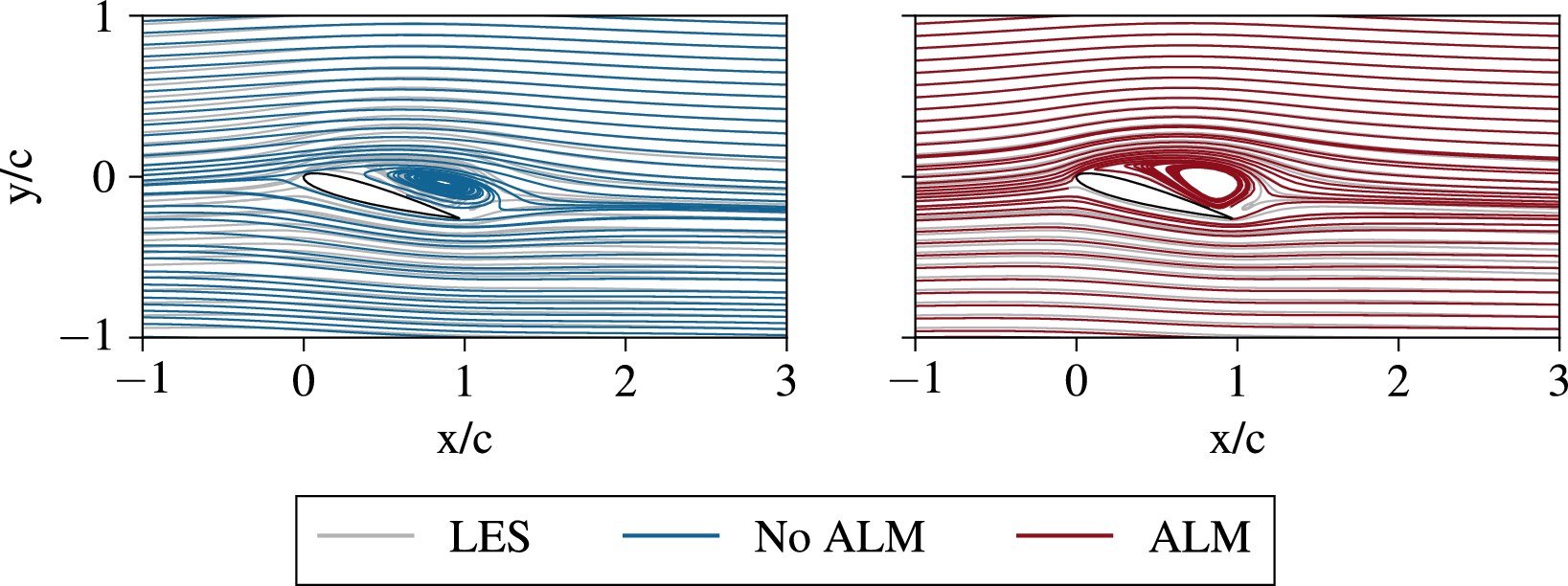
Figure 13. Long description
The image consists of two horizontal panels with identical axes. The x-axis is labeled x forward slash c ranging from negative 1 to 3. The y-axis is labeled y forward slash c ranging from negative 1 to 1. At the center of each panel is a tilted airfoil shape.
In the left panel, blue streamlines represent the soft-constrained No A L M model overlaid on grey L E S reference streamlines. The blue lines closely follow the grey lines in the laminar regions but show a large recirculating vortex bubble directly above the trailing edge of the airfoil, centered near x forward slash c equals 1.
In the right panel, red streamlines represent the hard-constrained A L M model overlaid on the same grey L E S reference. The red lines show a tighter, more elongated recirculation zone above the airfoil compared to the blue model. The red streamlines appear to deviate slightly more from the grey reference lines in the wake region downstream of the airfoil.
A legend at the bottom identifies the grey line as L E S, the blue line as No A L M, and the red line as A L M.
The effects of the hard constraints are most notable toward the leading edge of the airfoil, where, without them, the PINN is unable to get the correct location of the stagnation point. With hard constraints, the stagnation point matches nearly perfectly with the reference LES dataset. Downstream in the recirculation region behind the airfoil, a similar pattern emerges where the hard-constrained PINN predictions are in strong agreement with the LES data. The key takeaway here is that with the hard constraints, the curvature of the airfoil is properly captured in the solution, ensuring the predictions of other quantities, such as pressure, are physically consistent and governed by the geometry.
4.3.3. Predicting pressure
Unlike the other quantities on the surface of the airfoil, the pressure acts as the only driven quantity, as we do not prescribe any pressure-related boundary conditions. Figure 14 makes the same comparison as in Section 4.3.2 for the surface pressure. Here, we observe that without hard constraints, the pressure remains approximately constant at
$ {C}_p\approx -0.2 $
 around the entire airfoil. Even without the reference data, we can assume this is unphysical for this type of flow and is a product of the PINN not capturing the curvature of the airfoil correctly, and the surface points, where predictions are generated, are not where the PINN believes the geometry to be. When we apply hard constraints, after
$ x/c=0.2 $
around the entire airfoil. Even without the reference data, we can assume this is unphysical for this type of flow and is a product of the PINN not capturing the curvature of the airfoil correctly, and the surface points, where predictions are generated, are not where the PINN believes the geometry to be. When we apply hard constraints, after
$ x/c=0.2 $
 , the pressure largely recovers to the reference data without any explicit data or boundary conditions enforcing this. This improvement in the driven quantities highlights the importance of proper enforcement of the boundary conditions to capture the geometry.
PINN surface pressure coefficient,
$ {C}_p $
 , predictions comparison between soft and hard (ALM) constraints. Reference surface pressure coefficient provided from L10 dataset.
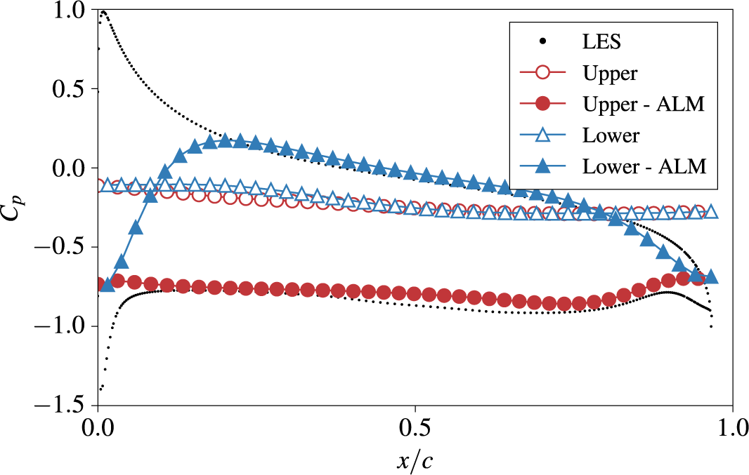
Figure 14. Long description
The X-axis represents the normalized chord position x forward slash c, ranging from 0.0 to 1.0. The Y-axis represents the pressure coefficient C sub p, ranging from negative 1.5 to 1.0.
* The L E S reference data is shown as a black dotted line, forming a large loop with a high peak near the leading edge (x forward slash c equals 0) and a narrow closure at the trailing edge.
* Upper surface data: The ‘Upper’ series (open pink circles) follows a nearly horizontal path near C sub p equals negative 0.2. The ‘Upper - A L M’ series (solid pink circles) shows a significant downward shift, following a horizontal path near C sub p equals negative 0.8.
* Lower surface data: The ‘Lower’ series (open blue triangles) is nearly horizontal near C sub p equals negative 0.1. The ‘Lower - A L M’ series (solid blue triangles) shows a complex curve that starts at negative 0.75, rises to a peak of 0.2 at x forward slash c equals 0.25, and then gradually declines toward the trailing edge.
A legend in the top right corner identifies the five data series: L E S (black dot), Upper (open pink circle), Upper - A L M (solid pink circle), Lower (open blue triangle), and Lower - A L M (solid blue triangle).
As for the points where
$ x/c<0.2 $
 , this can be attributed to the fact that, with PINNs, the surface collocation points used for inference may not coincide with the pressure or suction peaks. For example, in the ALM case, the pressure coefficient range is from
$ -0.90 $
, this can be attributed to the fact that, with PINNs, the surface collocation points used for inference may not coincide with the pressure or suction peaks. For example, in the ALM case, the pressure coefficient range is from
$ -0.90 $
 to
$ 0.77 $
to
$ 0.77 $
 . Whilst this still does not match the reference data exactly, it is much closer than the range of values in Figure 14. Furthermore, the location of the pressure peak is at
$ \left(-0.02,-0.05\right) $
. Whilst this still does not match the reference data exactly, it is much closer than the range of values in Figure 14. Furthermore, the location of the pressure peak is at
$ \left(-0.02,-0.05\right) $
 , which highlights that the training methodology can recover pressure from sparse velocity measurements, but some caution is required when interpreting the models’ predictions.
The other aspect of predicting pressure not discussed so far in the results is the coupling of P with
$ \phi $
 . To reduce the number of unknowns, we apply the Helmholtz decomposition in Equation 2.2 and group the potential component with the pressure. To recover Equation 3.1 from Equation 3.2, we must assume that the
$ \phi \equiv {\phi}_{\infty } $
. To reduce the number of unknowns, we apply the Helmholtz decomposition in Equation 2.2 and group the potential component with the pressure. To recover Equation 3.1 from Equation 3.2, we must assume that the
$ \phi \equiv {\phi}_{\infty } $
 so that the PINN predicted pressure matches the reference pressure. However, we cannot be certain that this is true as the two components cannot be easily separated. Foures et al. (Reference Foures, Dovetta, Sipp and Schmid2014) suggest that the contribution of
$ \phi $
so that the PINN predicted pressure matches the reference pressure. However, we cannot be certain that this is true as the two components cannot be easily separated. Foures et al. (Reference Foures, Dovetta, Sipp and Schmid2014) suggest that the contribution of
$ \phi $
 is small and that
$ \nabla \phi \approx -\nabla k $
is small and that
$ \nabla \phi \approx -\nabla k $
 and that (
$ \overline{P}-\phi $
and that (
$ \overline{P}-\phi $
 ) would be very close to the true pressure,
$ \overline{P} $
) would be very close to the true pressure,
$ \overline{P} $
 . When analysing the other PINN models, in particular where we do not have reliable reference data from the experiments, this method can give us more trust in the predicted pressure fields.
4.4. PINNs with transfer learning to PIV data
With the LES models acting as a validation of the methodology, we can now apply the same techniques to the experimental PIV data. We can directly compare the capabilities of transfer learning to the original baseline model in Section 4.1. As with applying transfer learning to LES, all models follow Algorithm 2 and use the parameters outlined in Section 3.
4.4.1.
$ P75-R{75}_b $

Figure 15 outlines the predicted fields for the driving quantities in this PINN setup. From this figure, we can make two comparisons, firstly to the reference data, Figure 3, used in training and secondly to the initial baseline attempt without transfer learning in Figures 8 and 9. Starting with the reference data, we can see a good agreement for both velocity components. Like the LES transfer learning models, the PINN can accurately modify the recirculation region, as indicated by the zero velocity streamline in the reference data. In this region, we can also see how the PINN can smooth discontinuous data without losing information. These sorts of discontinuities come from post-processing issues of the PIV when multiple cameras or light sources are present. Alongside obtaining otherwise unknown quantities of the flow, PINNs can provide better analysis of experimental data.
PINN predicted fields from model
$ P75-R{75}_b $
 of the driving quantities for each velocity component,
$ \overline{U}\&\overline{V} $
of the driving quantities for each velocity component,
$ \overline{U}\&\overline{V} $
 , and their respective errors to reference P75 dataset. For
$ \overline{U} $
, and their respective errors to reference P75 dataset. For
$ \overline{U} $
 , the dashed line indicates the edge of the recirculation region from the experimental data.
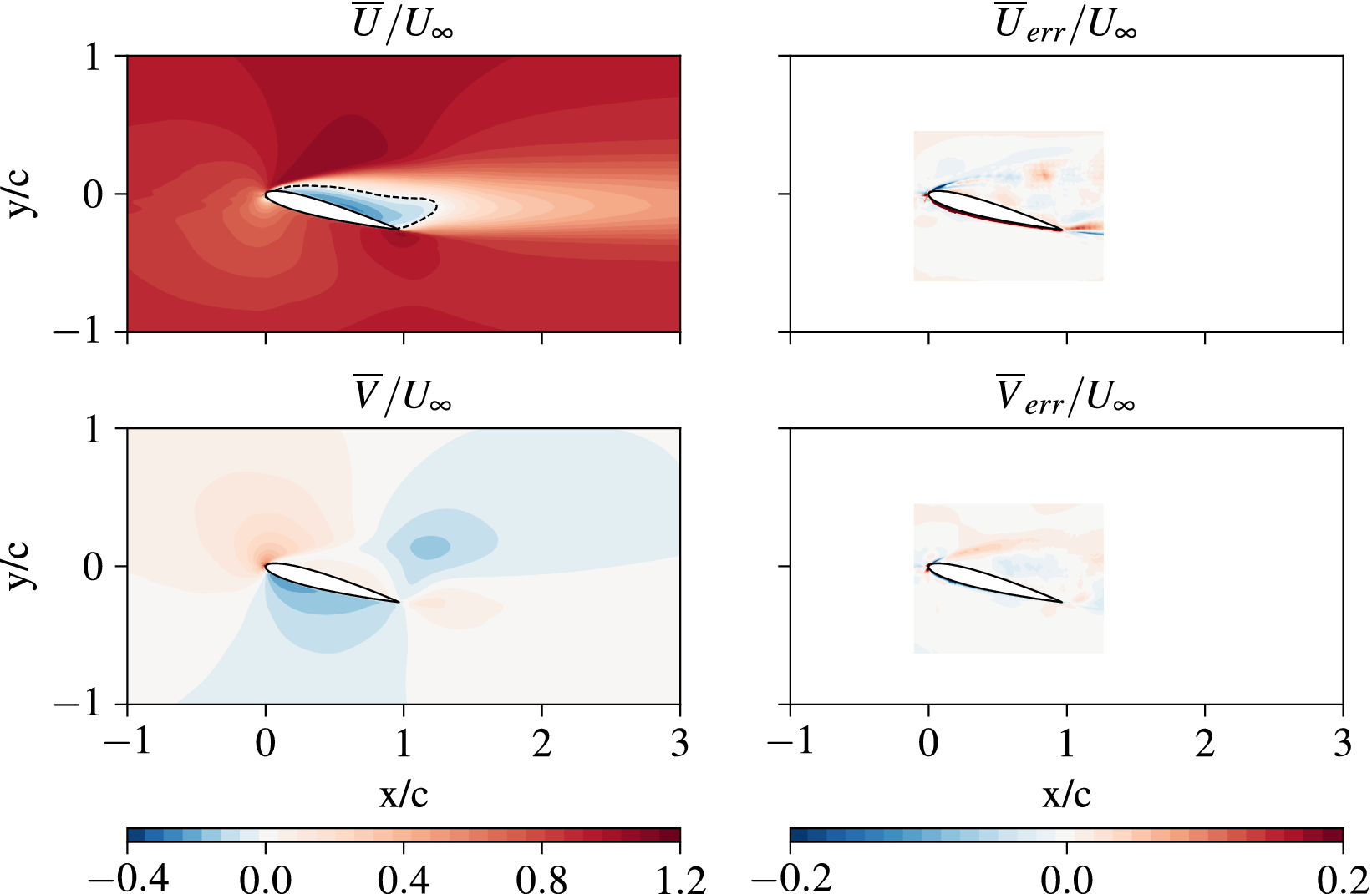
Figure 15. Long description
A four-panel heatmap display. All panels share an x-axis labeled x forward slash c ranging from negative 1 to 3 and a y-axis labeled y forward slash c ranging from negative 1 to 1.
Top-left panel: Labeled U-bar over U-infinity. It shows a red-dominant field representing horizontal velocity. A white airfoil shape is centered at the origin. A dashed line outlines a recirculation region immediately behind and above the airfoil. The wake extends to the right in lighter red and white tones.
Top-right panel: Labeled U-bar sub err over U-infinity. It shows the error for the horizontal velocity. The field is mostly white, indicating low error, with small patches of light blue and red concentrated near the airfoil surface and trailing edge.
Bottom-left panel: Labeled V-bar over U-infinity. It shows vertical velocity. Red regions (positive velocity) are located above the airfoil leading edge and below the trailing edge. Blue regions (negative velocity) are located below the leading edge and above the trailing edge.
Bottom-right panel: Labeled V-bar sub err over U-infinity. It shows the error for vertical velocity. Similar to the top-right, the field is predominantly white with minor red and blue fluctuations near the airfoil boundary.
Two color bars are at the bottom. The left bar for velocity fields ranges from negative 0.4 (dark blue) to 1.2 (dark red). The right bar for error fields ranges from negative 0.2 (dark blue) to 0.2 (dark red) with 0.0 as white.
When comparing to the baseline PIV model, we can see that using transfer learning suppresses the presence of unphysical predictions by the PINN. Firstly, when comparing to the results in Figure 8, we do not get a secondary recirculation region within the shear layer of the leading edge. In the near-wall region, we see a nearly identical error profile on the airfoil’s pressure side to the
$ P{75}_b $
 case. Given the relatively constant distance of the error from the airfoil’s surface, it is reasonable to assume that this is from laser reflections and erroneous vectors in this region of the dataset, reinforcing the conclusions of Section 4.1. As the
$ P{75}_b $
case. Given the relatively constant distance of the error from the airfoil’s surface, it is reasonable to assume that this is from laser reflections and erroneous vectors in this region of the dataset, reinforcing the conclusions of Section 4.1. As the
$ P{75}_b $
 model did not exhibit any major unphysical features here; it reinforces the point that this error is driven by the reference data. The less complex physics on the pressure side of the airfoil allow the PINN to more easily correct this error over the suction side, which requires additional support. For the suction side, the error is much lower in the transfer learning case. This indicates that the PINN can more accurately predict the near-wall region for flows with an adverse pressure gradient by providing an initial guess from a baseline model.
Finally, we can see from the error plots a reduction in the error around the leading edge of the airfoil. The improved shape of the contours at the leading edge suggests a more accurately resolved stagnation point compared to the baseline attempt. The impact of this improvement likely contributes to the aforementioned enhancements to other features of the velocity fields.
The improvements at the airfoil’s leading edge also result in more physical results for the driven quantities. For pressure, we can see the improvements eliminate the detachment of the stagnation point to a position forward of the airfoil. Additionally, in Figure 9, some discontinuities can be seen in the low-pressure zone away from the airfoil. In Figure 16, we see a smoother and more continuous variation in the pressure. As for the Reynolds shear stresses, there are significant improvements over the original baseline. The discontinuous and patchy distribution of the stresses through the shear layer is removed and approximates the experimental distribution. We do not want a perfect match for this quantity, as the lack of stress in the shear layer from the leading edge is not physical. As previously stated, this is likely an artefact of the experimental data, and the PINN correcting this data indicates that it has learned the underlying physics of the problem, not simply overfitting the model to the data provided. However, the model suppresses the peak magnitude of the stresses when compared to both the baseline and reference data. The three-dimensional nature of the flow is likely to be the source of discrepancy since the PINN is trying to fit the data to two-dimensional equations (Cadambi Padmanaban et al., Reference Cadambi Padmanaban, Ganapathisubramani and Symon2026).
PINN predicted fields from model
$ P75-R{75}_b $
 of the driven quantities, including the pressure coefficient,
$ {C}_p $
of the driven quantities, including the pressure coefficient,
$ {C}_p $
 , and Reynolds shear stress,
$ \overline{u^{\prime }{v}^{\prime }} $
, and Reynolds shear stress,
$ \overline{u^{\prime }{v}^{\prime }} $
 .
.

Figure 16. Long description
Two horizontal panels display fluid dynamics data. Both panels share an x all over c horizontal axis from negative 1 to 3 and a y all over c vertical axis from negative 1 to 1. An airfoil is centered at the origin, angled downward.
Left Panel: Pressure coefficient C sub p. A color scale below ranges from negative 1.4 in dark blue to 1.0 in dark red. A high-pressure red region is concentrated at the leading edge stagnation point. A low-pressure blue region covers the upper surface of the airfoil, extending into the flow field above and behind it.
Right Panel: Reynolds shear stress u prime v prime overline. A color scale below ranges from negative 5 to 5 times 10 to the negative 2 power. The field is mostly neutral gray. A positive red shear layer originates from the upper surface leading edge and extends into the wake. A negative blue shear layer originates from the trailing edge and extends horizontally to the right.
4.5. Performance overview of transfer learning
To supplement these results, Figure 17 provides a quantitative overview of the performance boost expected when using transfer learning for a given dataset and baseline model. A direct comparison between these models trained on different datasets is not valid, but all the results are grouped here to show the general trends between the transfer learning cases presented in this work. For each model outlined in Table 4 and high-fidelity models in Table 3, the combined RMSE is computed for both the driving and driven variables, respectively, where the ground truth is available. Notably, this excludes
$ {C}_p $
 from all P75 models. Therefore, comparisons between the accuracy of models using varying datasets are invalid and are only qualitative in terms of the trends found. The combined RMSE is defined as,

where
$ i $
 represents the number of reference points and
$ n $
represents the number of reference points and
$ n $
 is the number of quantities. The RMSE is evaluated with the complete reference data inside the data domain defined in Table 4.
Summary of performance gains when using transfer learning over the baseline algorithm, only for driving and driven variables, respectively.
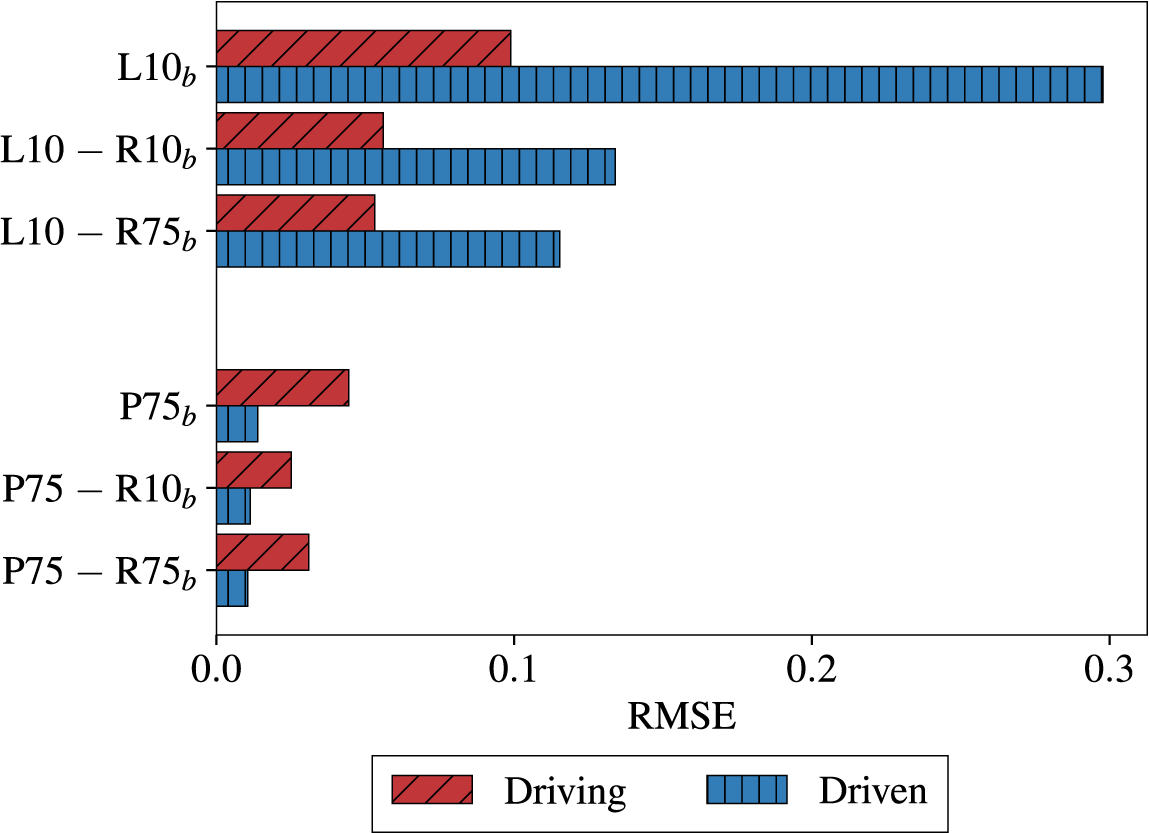
Figure 17. Long description
The horizontal bar chart uses an x-axis labeled R M S E with a scale from 0.0 to 0.3. The y-axis lists six configurations divided into two groups. A legend at the bottom identifies pink bars with diagonal hatching as Driving and blue bars with vertical hatching as Driven.
Top Group (L configurations):
* L 10 sub b: Driving is approximately 0.10 and Driven is approximately 0.30.
* L 10 minus R 10 sub b: Driving is approximately 0.06 and Driven is approximately 0.14.
* L 10 minus R 75 sub b: Driving is approximately 0.05 and Driven is approximately 0.12.
Bottom Group (P configurations):
* P 75 sub b: Driving is approximately 0.04 and Driven is approximately 0.01.
* P 75 minus R 10 sub b: Driving is approximately 0.02 and Driven is approximately 0.01.
* P 75 minus R 75 sub b: Driving is approximately 0.03 and Driven is approximately 0.01.
Overall, the L configurations show significantly higher R M S E values than the P configurations, with Driven variables consistently showing higher error than Driving variables in the L group, while the reverse is true in the P group.
In addition to testing transfer learning with a matched Reynolds number between the RANS and respective high-fidelity dataset, we also considered the effects of applying this methodology with the mismatched Reynolds numbers in the models
$ L10-R{75}_b $
 and
$ P75-R{10}_b $
and
$ P75-R{10}_b $
 . The proposition for both models is that, given the identical geometries and similarities in the RANS eddy viscosity fields, it may be possible to repurpose a baseline model to avoid significant training time.
In both models, a small dependence on the quality of the baseline model was apparent, with any errors in the baseline propagating into the final model. This did not cause major differences between the two models for a given dataset, e.g.
$ L10-R{10}_b $
 and
$ L10-R{75}_b $
and
$ L10-R{75}_b $
 , but any minor discrepancies could only be attributed to the variations in the baseline model. Figure 17 reinforces these findings with the RMSE for the driven quantities being lowest for models initialized with the
$ R{75}_b $
, but any minor discrepancies could only be attributed to the variations in the baseline model. Figure 17 reinforces these findings with the RMSE for the driven quantities being lowest for models initialized with the
$ R{75}_b $
 baseline.
For the
$ P75-R{10}_b $
 , the consistency with the
$ P75-R{75}_b $
, the consistency with the
$ P75-R{75}_b $
 predictions highlights the robustness of the methodology. Additionally, by comparing the error of the two models to the reference PIV data, we could be certain of the errors associated with the PINN and those associated with the uncertainties in the reference data.
In all cases, transfer learning yielded a minimum improvement of 18% across all variables and as high as 61% for the driven variables in the
$ L10-R{75}_b $
 case. The key takeaway from this analysis is that to obtain unknown quantities accurately, the quality of the baseline model supersedes the necessity to match the Reynolds number.
5. Conclusion
To summarize the work presented here, we have presented a transfer learning-based methodology for improving mean flow reconstruction using PINNs and sparse experimental measurements. We have demonstrated the robustness of the methodology by first applying it to a LES dataset and then to a higher Reynolds number PIV dataset, with consistent improvements in both cases. These results show that the combination of extensions presented here, transfer learning and hard constrained boundary conditions, helps to overcome the notable challenges within the PINN methodology and enable the recovery of other mean quantities, including pressure and Reynolds shear stress.
When applying our PIV dataset naively to a PINN model, we found only a reasonable agreement between the driving variables (
$ \overline{U}\&\overline{V} $
 ) and the original reference data. From the predicted Reynolds shear stresses, we identified that the source of this error was related to problems predicting eddy viscosity in a physically consistent manner. With transfer learning applied from a RANS-trained PINN baseline model, we observed significant improvements to the prediction of both the driving and the driven quantities. This improvement in the driven quantity predictions indicates that the PINN is learning the underlying physics from the equations and not overfitting the data. Additionally, the ability to derive physical meaning from the quantities learnt indirectly from the model helps improve interpretability.
Alongside this new methodology, we also studied the importance of matching all physical constraints on the flow, including the no-slip boundary condition. Here, we used an augmented Lagrangian method to update a Lagrange multiplier on each boundary collocation point to increase the effective weighting of that point to the total loss of the PINN. This extension to the constraints resulted in a reduction of the surface velocity by two orders of magnitude. When comparing the surface pressure, the ALM PINN had a much closer agreement to the reference LES data beyond
$ x/c=0.2 $
 , where the soft-constrained PINN predicted a near-constant value across the airfoil surface. One possible extension to this would be to investigate the effects of different optimizers and whether more advanced optimizers, such as L-BFGS, can remove deviations, in particular at the leading edge of the airfoil.
Furthermore, we showcased that this methodology is repeatable across different datasets, and transfer learning is applicable between datasets of varying Reynolds numbers. Due to the similarity in the eddy viscosity fields, the transferability between Reynolds numbers indicates that the emphasis should be on creating a higher accuracy baseline model instead of matching the specific Reynolds number of each experimental case in a dataset. This method also helps to reduce the computational cost, particularly over larger datasets. Further exploration is required to verify the extent of this transferability between Reynolds numbers and whether this methodology is appropriate to transfer between similar geometries, for example, going from a NACA 0012 airfoil to a NACA 0020.
Data availability statement
Data published in this article are available from the University of Southampton repository at https://doi.org/10.5258/SOTON/D3539 (Toma et al., Reference Toma, Ganapathisubramani and Symon2026).
Acknowledgements
We are grateful for the technical assistance of Uttam Cadambi Padmanaban for producing the LES data and the University of Southampton’s High Performance Computing Facility, IRIDIS X, for the technical support and computational resources used in the completion of this work. Artificial intelligence tools (ChatGPT) were used only for writing refinement in this research.
Author contribution
Conceptualization: C.T., B.G., S.S.; Data curation: C.T.; Formal analysis: C.T.; Funding acquisition: B.G., S.S.; Investigation: C.T.; Methodology: C.T.; Project administration: C.T., B.G., S.S.; Software: C.T.; Supervision: B.G., S.S.; Visualization: C.T.; Writing - original draft: C.T.; Writing - review & editing: C.T., B.G., S.S.; C.T. contributed to the implementation of the PINN codes, creation of the associated training procedures, analysing the results and writing several drafts. B.G. and S.S. were responsible for conceptualization, funding acquisition, editing of drafts and project management.
Funding statement
We gratefully acknowledge funding from the School of Engineering at the University of Southampton and EPSRC grant no. EP/W524621/1 for CT’s PhD studentship.
Competing interests
The authors declare no conflict of interest.
Ethical standard
The research meets all ethical guidelines, including adherence to the legal requirements of the study country.
Appendix: LES data generation and validation
A.1. Generating dataset
A high-fidelity computational dataset is generated by performing wall-resolved large eddy simulations (WRLES) of a flow past a NACA 0012 airfoil at
$ \alpha =15{}^{\circ} $
 using OpenFOAM (Weller et al., Reference Weller, Tabor, Jasak and Fureby1998). The governing equations are solved with the pimpleFoam solver, which combines the PISO (pressure-implicit with splitting of operators) (Issa, Reference Issa1986) and SIMPLE (semi-implicit pressure-linked equations) algorithms (Patankar and Spalding, Reference Patankar and Spalding1972). This combination allows for the use of larger time steps, thereby reducing the overall computational cost. The pimpleFoam solver works by seeking a quasi-steady approximation of the solution at each time step, achieved through multiple “inner” iterations. The converged solution at one time step is then propagated to the next time step.
Turbulence modeling is performed using the wall-adapting local eddy-viscosity (WALE) model (Nicoud and Ducros, Reference Nicoud and Ducros1999). This model is well-suited for capturing transition and is less dissipative than the traditional Smagorinsky model (Duan and Wang, Reference Duan and Wang2024), making it more effective in preserving small-scale turbulence structures. The airfoil has a chord of
$ c=1m $
 with a blunt trailing edge and is surrounded by an O-grid with a diameter of
$ {L}_x/c=120 $
with a blunt trailing edge and is surrounded by an O-grid with a diameter of
$ {L}_x/c=120 $
 . The pressure and suction sides of the airfoil are discretized using
$ 200 $
. The pressure and suction sides of the airfoil are discretized using
$ 200 $
 points each, and the blunt trailing edge is discretized using
$ 15 $
points each, and the blunt trailing edge is discretized using
$ 15 $
 points. The domain extends in the spanwise direction by
$ {L}_z/c=1 $
points. The domain extends in the spanwise direction by
$ {L}_z/c=1 $
 , as the flow transitions to a three-dimensional state at this Reynolds number with a dominant spanwise wavelength of
$ {\lambda}_z\approx c/3 $
, as the flow transitions to a three-dimensional state at this Reynolds number with a dominant spanwise wavelength of
$ {\lambda}_z\approx c/3 $
 (Gupta et al., Reference Gupta, Zhao, Sharma, Agrawal, Hourigan and Thompson2023). The span is discretized using
$ 25 $
(Gupta et al., Reference Gupta, Zhao, Sharma, Agrawal, Hourigan and Thompson2023). The span is discretized using
$ 25 $
 points with a spacing of
$ {\Delta}_z=0.04c $
points with a spacing of
$ {\Delta}_z=0.04c $
 , giving a total mesh size of
$ \mathrm{2,266,000} $
, giving a total mesh size of
$ \mathrm{2,266,000} $
 cells.
The incoming flow is set at
$ {U}_{\infty }=1m/s $
 . The Reynolds number is fixed at
$ {\mathit{\operatorname{Re}}}_c=\mathrm{10,000} $
. The Reynolds number is fixed at
$ {\mathit{\operatorname{Re}}}_c=\mathrm{10,000} $
 by setting the kinematic viscosity to
$ \nu ={10}^{-4}{m}^2/s $
by setting the kinematic viscosity to
$ \nu ={10}^{-4}{m}^2/s $
 . The first grid point is located at
$ {y}_1=0.5 mm $
. The first grid point is located at
$ {y}_1=0.5 mm $
 , resulting in an average
$ {y}^{+}=0.27 $
, resulting in an average
$ {y}^{+}=0.27 $
 . The gradients are computed using a second-order accurate central differencing scheme. The velocity term is discretized using a limited central differencing scheme that applies an upwind method in regions of strong gradients. The turbulence variable
$ \tilde{\nu} $
. The gradients are computed using a second-order accurate central differencing scheme. The velocity term is discretized using a limited central differencing scheme that applies an upwind method in regions of strong gradients. The turbulence variable
$ \tilde{\nu} $
 is discretized using an unbounded second-order scheme. The equations for scalar variables are solved using a preconditioned conjugate gradient (PCG) solver, while vector variables are solved using a preconditioned bi-conjugate gradient stabilized (PBiCGStab) solver. A second-order implicit scheme is used for time-stepping. The time step is set to
$ \Delta t=0.001 $
is discretized using an unbounded second-order scheme. The equations for scalar variables are solved using a preconditioned conjugate gradient (PCG) solver, while vector variables are solved using a preconditioned bi-conjugate gradient stabilized (PBiCGStab) solver. A second-order implicit scheme is used for time-stepping. The time step is set to
$ \Delta t=0.001 $
 , resulting in a maximum Courant number of
$ Co\approx 2 $
, resulting in a maximum Courant number of
$ Co\approx 2 $
 .
.
A mixed boundary condition is applied for velocity and the turbulence variable, switching between a fixed-value Dirichlet type and a fixed-gradient Neumann type based on the sign of the velocity flux. A pressure outlet boundary is imposed along the circumference of the domain, while the airfoil surface is treated as a no-slip boundary. Since
$ {y}^{+}<1 $
 , the viscous sublayer is fully resolved, eliminating the need for wall functions. After the initial transient phase, the flow is averaged over 565 eddy turnover times
$ {T}^{+} $
, the viscous sublayer is fully resolved, eliminating the need for wall functions. After the initial transient phase, the flow is averaged over 565 eddy turnover times
$ {T}^{+} $
 , where one eddy turnover time is defined as
$ {T}^{+}=c/{U}_{\infty } $
, where one eddy turnover time is defined as
$ {T}^{+}=c/{U}_{\infty } $
 . The integral time scale
$ {T}_i $
. The integral time scale
$ {T}_i $
 is estimated by placing a probe in the wake of the airfoil at approximately
$ 0.2c $
is estimated by placing a probe in the wake of the airfoil at approximately
$ 0.2c $
 downstream of the trailing edge and along the leading-edge shear layer, yielding
$ {T}_i=0.3 $
downstream of the trailing edge and along the leading-edge shear layer, yielding
$ {T}_i=0.3 $
 . Based on this, a sampling frequency of
$ {f}_s=1/0.3=3.33 $
. Based on this, a sampling frequency of
$ {f}_s=1/0.3=3.33 $
 Hz is chosen, resulting in approximately
$ 1800 $
Hz is chosen, resulting in approximately
$ 1800 $
 instantaneous snapshots of velocity, which is then used to compute the time-averaged velocity field. This is span-averaged to obtain the final reference dataset.
A.2. Validating dataset
While several methods exist to validate the high-fidelity dataset, we present the frequency spectrum of the integrated lift coefficient
$ {C}_L $
 , defined as

where
$ \rho $
 is the fluid density,
$ {U}_{\infty } $
is the fluid density,
$ {U}_{\infty } $
 is the freestream velocity,
$ S $
is the freestream velocity,
$ S $
 is the span of the wing. The integrated lift coefficient is sampled at a frequency of
$ {f}_s=10 $
is the span of the wing. The integrated lift coefficient is sampled at a frequency of
$ {f}_s=10 $
 kHz. The corresponding frequency spectrum is shown in Figure A1. From this, the Strouhal number (
$ St $
kHz. The corresponding frequency spectrum is shown in Figure A1. From this, the Strouhal number (
$ St $
 ) is estimated as

where
$ f $
 is the dominant frequency.
LES lift spectra of a NACA 0012 airfoil at
$ \alpha $
 = 15° and Reynolds number, Re = 10,000.
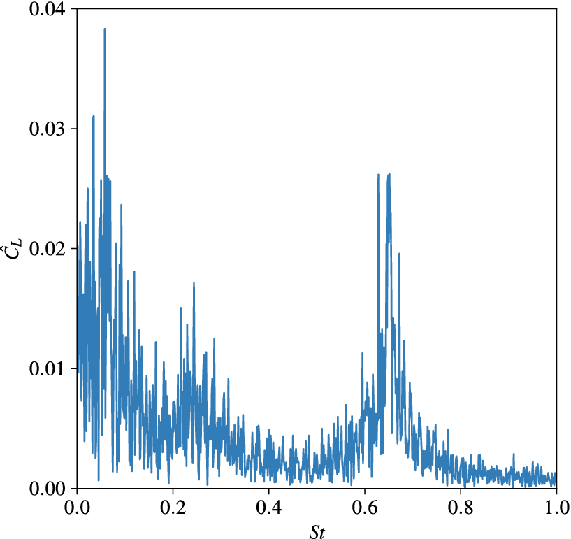
Figure 18. Long description
The x-axis represents the Strouhal number S t ranging from 0.0 to 1.0. The y-axis represents the lift coefficient C sub L hat ranging from 0.00 to 0.04. The data is plotted as a highly oscillatory blue line. Starting from the left, there is a broad, high-intensity region of fluctuations between S t equals 0.0 and 0.2, reaching a maximum peak of approximately 0.038 at S t equals 0.06. Following this, the amplitude of fluctuations decreases significantly, reaching a local minimum around S t equals 0.45. A second, narrower peak emerges between S t equals 0.6 and 0.7, reaching a height of approximately 0.026. Beyond S t equals 0.7, the signal decays into low-amplitude noise as it approaches S t equals 1.0.
The Strouhal number of the peak frequency is
$ St=0.6515 $
 , which closely agrees with the value reported in Rolandi et al. (Reference Rolandi, Smith, Amitay, Theofilis and Taira2025), where the authors obtained
$ St=0.675 $
, which closely agrees with the value reported in Rolandi et al. (Reference Rolandi, Smith, Amitay, Theofilis and Taira2025), where the authors obtained
$ St=0.675 $
 for a similar case at
$ 14{}^{\circ} $
for a similar case at
$ 14{}^{\circ} $
 angle of attack and the same Reynolds number. Furthermore, the characteristic three-peak structure in the lift coefficient spectrum, previously observed in Rolandi et al. (Reference Rolandi, Smith, Amitay, Theofilis and Taira2025), is also present in our results. Additionally, the
$ U=0 $
angle of attack and the same Reynolds number. Furthermore, the characteristic three-peak structure in the lift coefficient spectrum, previously observed in Rolandi et al. (Reference Rolandi, Smith, Amitay, Theofilis and Taira2025), is also present in our results. Additionally, the
$ U=0 $
 contour, as shown in Figure 3, outlines a small separation bubble slightly downstream of the leading-edge separation point, which is a known characteristic of the flow at this Reynolds number, as also noted in Figure 4 in Rolandi et al. (Reference Rolandi, Smith, Amitay, Theofilis and Taira2025).
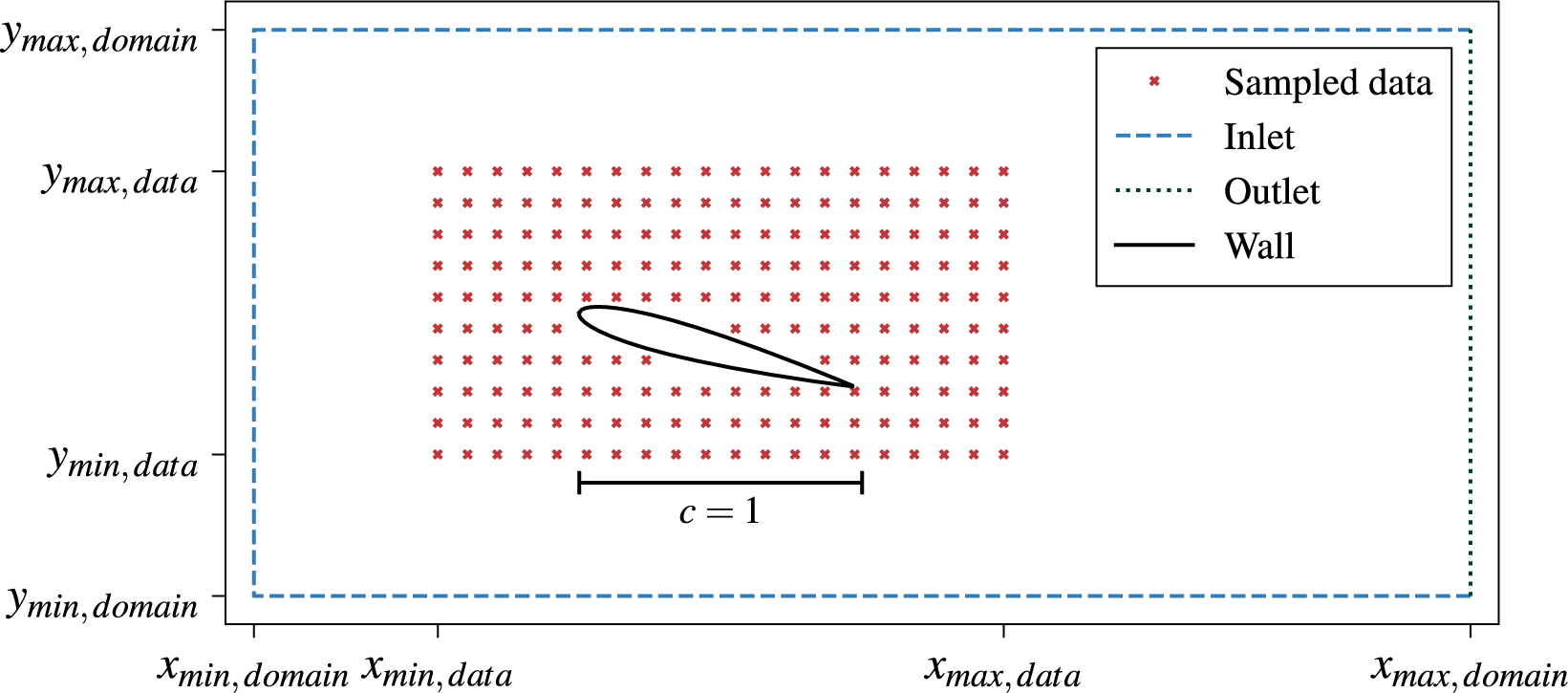

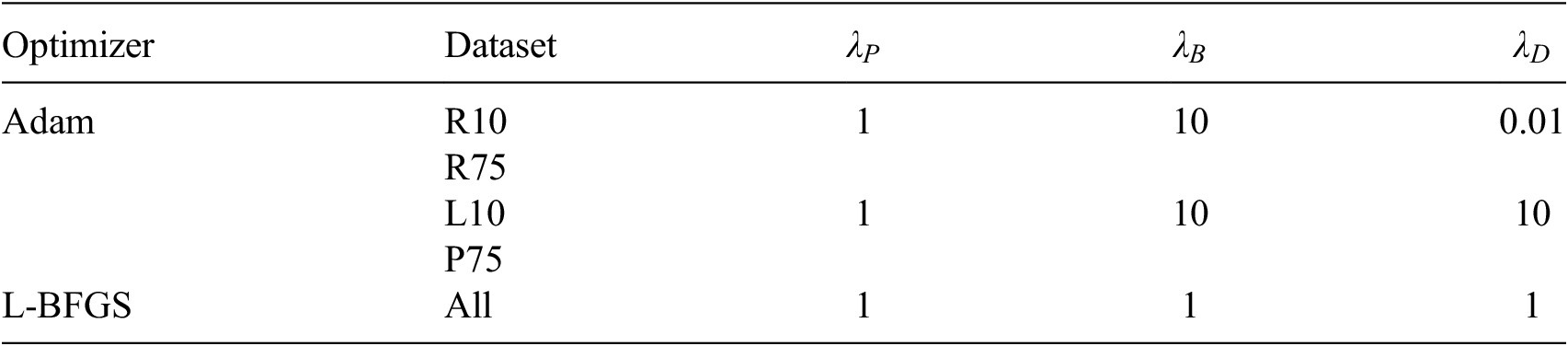
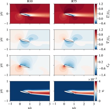


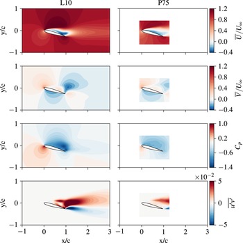


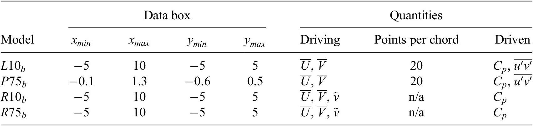
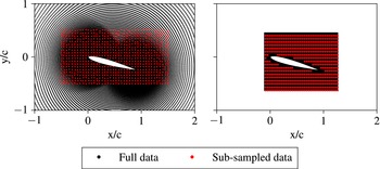
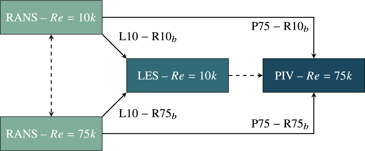

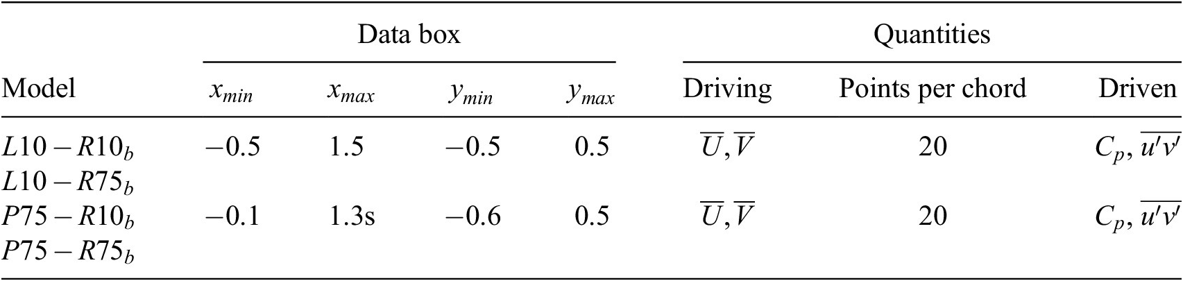

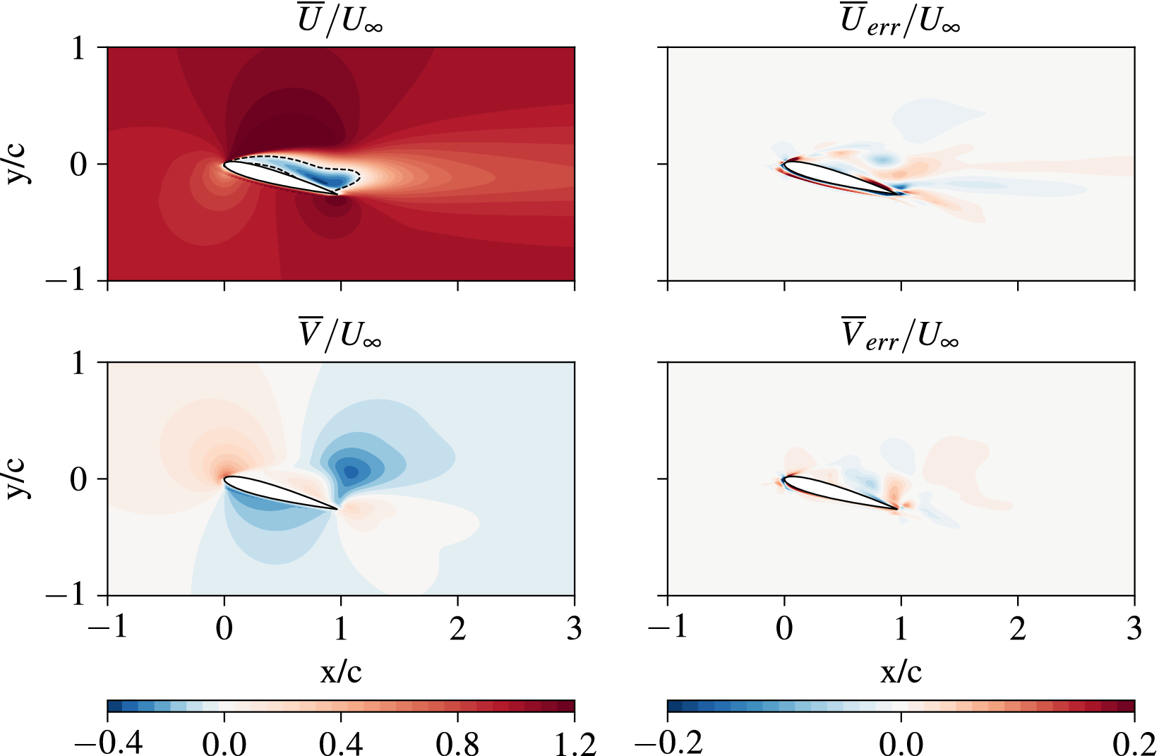


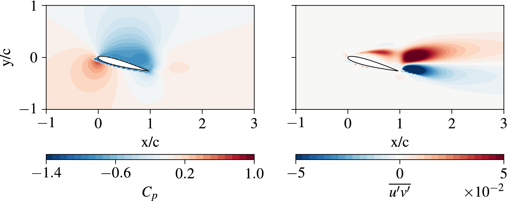


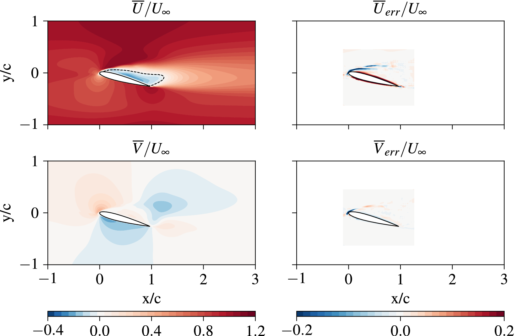


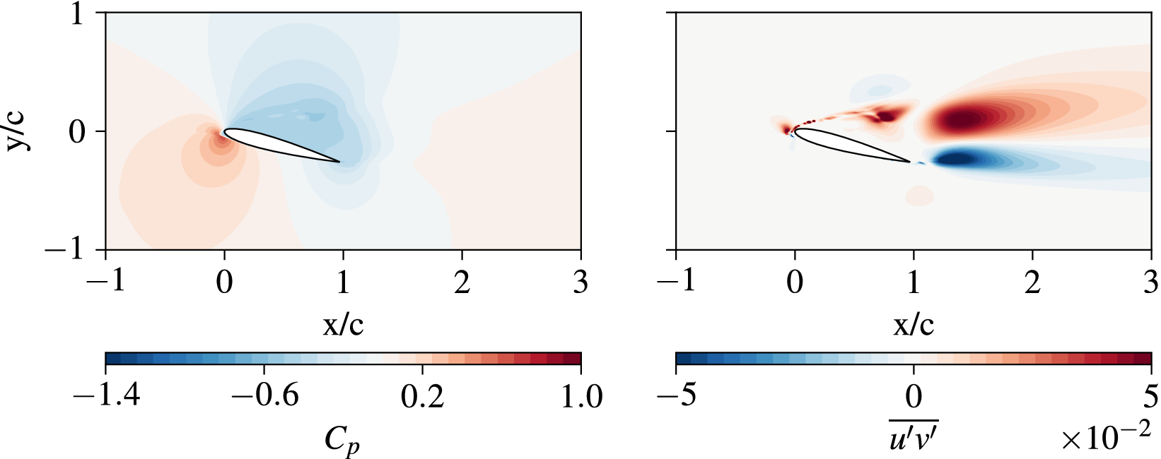


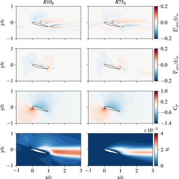


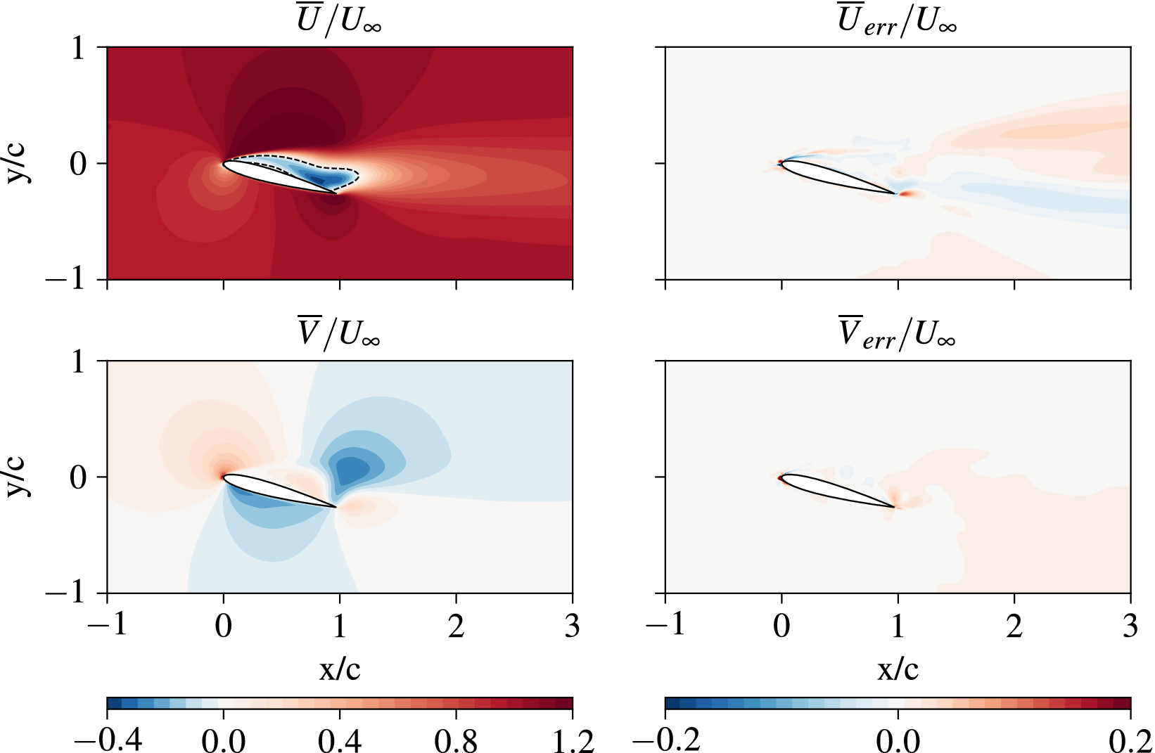


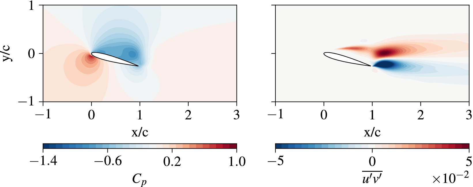


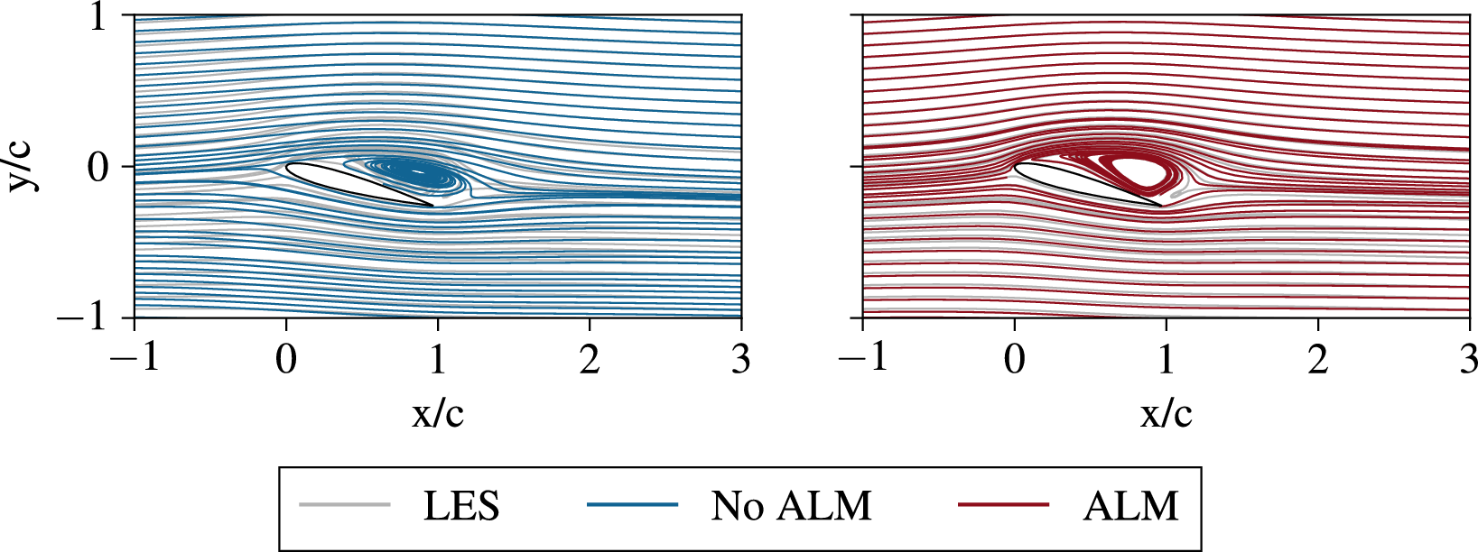
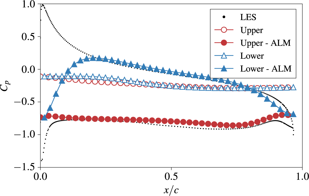

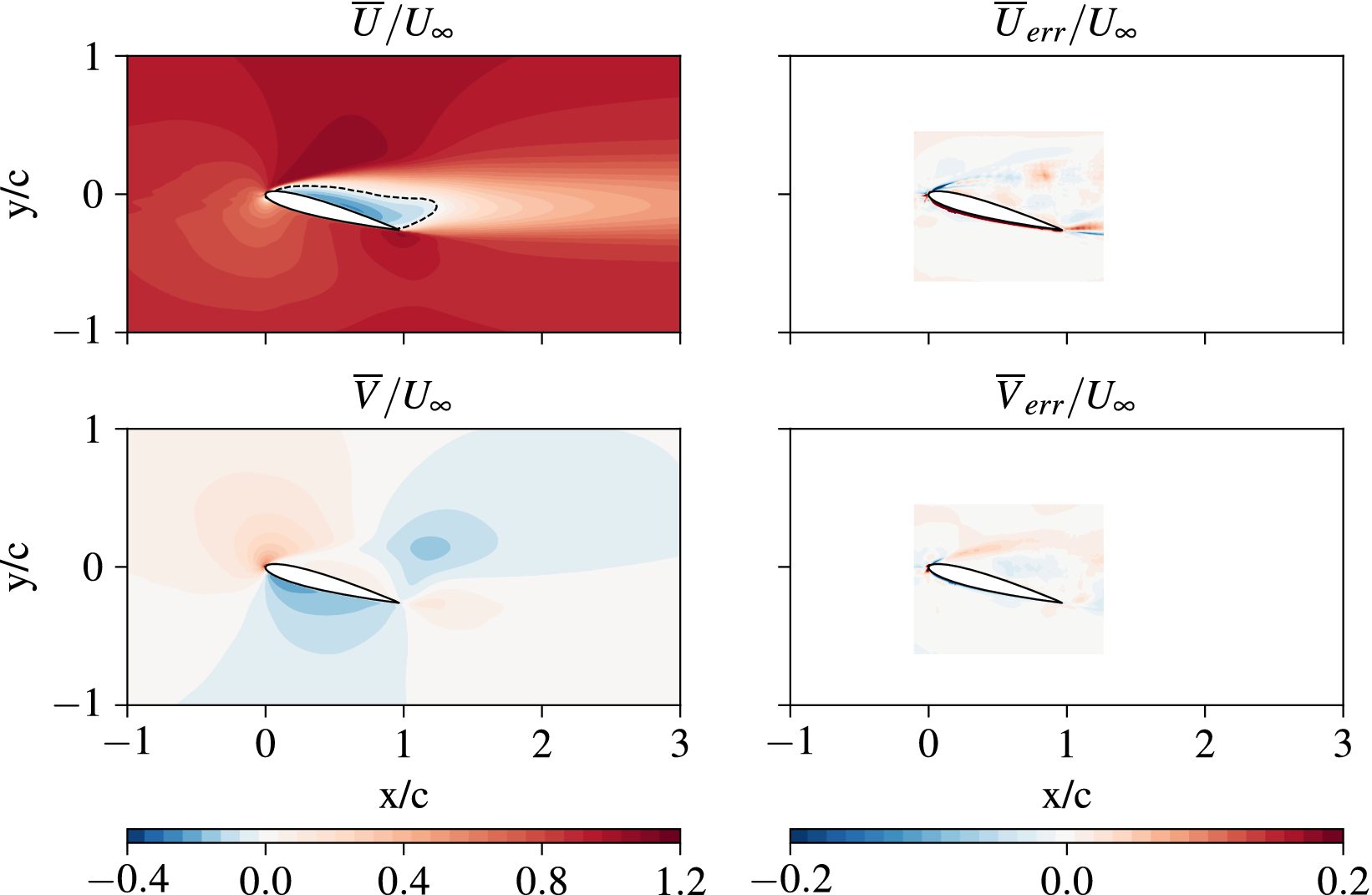


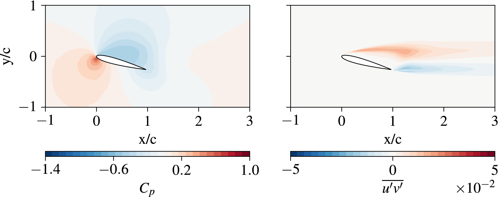


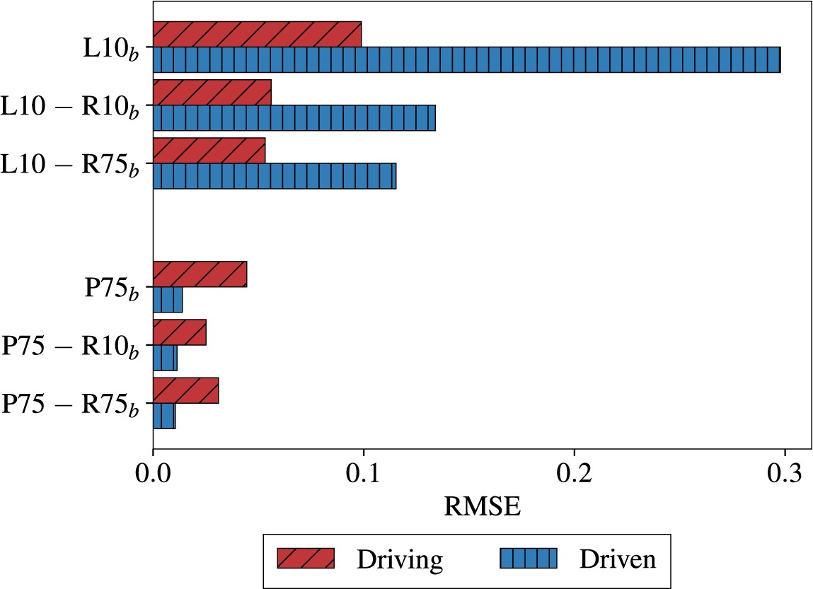
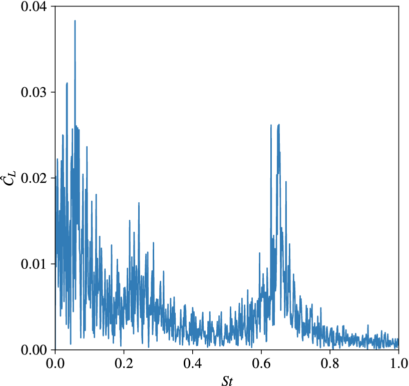


 Open access


Comments
No Comments have been published for this article.