


1. Introduction
A type I X-ray burst is rapid nuclear burning on the surface of a neutron star (NS) (e.g. Lewin van Paradijs, & Taam, Reference Lewin, van Paradijs and Taam1993). Type I X-ray bursts happen when the accumulated ‘nuclear fuel’ accreted from the donor star onto the surface of the NS is sufficiently hot. In some cases, the radiation pressure becomes large enough to overcome the gravity of the NS, causing the photosphere to expand. This is followed by fallback of the photosphere after extending to its outermost point. This process of expansion and contraction of the photosphere is well characterised by double-peaked soft X-ray light curves. These particular type I X-ray bursts are called photospheric radius expansion (PRE) bursts.
According to Galloway et al. (Reference Galloway2020), there are hitherto 115 recognised PRE bursters (see https://burst.sci.monash.edu/ sources), which are all low mass X-ray binaries (LMXBs). PRE bursts can serve as standard candles (Basinska et al. Reference Basinska, Lewin, Sztajno, Cominsky and Marshall1984) based on the assumption that the luminosity of PRE bursts stays at the Eddington limit throughout the photospheric expansion and contraction. We refer to the distances estimated in this way as PRE distances. Using the standard assumption of spherically symmetric PRE burst emission, Galloway et al. (Reference Galloway2020) constrained PRE distances for 73 PRE bursters (23 of which only have upper limits of PRE distances, see Table 8 of Galloway et al. Reference Galloway2020) based on the theoretical Eddington luminosity calculated by Lewin et al. (Reference Lewin, van Paradijs and Taam1993). Hereafter, we refer to this spherically symmetric model as the simplistic PRE model, and the simplistic-PRE-model-based PRE distances as nominal PRE distances. Besides PRE models, a Bayesian framework has been recently developed to infer parameters, including the distance and the composition of nuclear fuel on the NS surface, for the type I X-ray burster SAX J1808.4-3658 (Goodwin et al. Reference Goodwin, Galloway, Heger, Cumming and Johnston2019), by matching the burst observables (such as burst flux and recurrence time) of non-PRE type I X-ray bursts with the prediction from a burst ignition model (Cumming & Bildsten Reference Cumming and Bildsten2000).
At least 43% of PRE bursters registered nominal PRE distances as their best constrained distances. The great usefulness of the simplistic PRE model calls for careful examination of its validity. There are several uncertainties in the simplistic PRE model. Firstly, according to Lewin et al. (Reference Lewin, van Paradijs and Taam1993), the Eddington luminosity measured by an observer at infinity
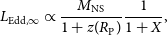 \begin{equation}L_{\textrm{Edd},\infty} \propto\frac{M_{\textrm{NS}}}{1+z(R_{\textrm{P}})} \frac{1}{1+X},\end{equation}
depends on the NS mass
 $M_{\textrm{NS}}$
and the gravitational redshift
$M_{\textrm{NS}}$
and the gravitational redshift
 $z(R_{\textrm{P}})=(1-2G_{\textrm{N}} M_{\textrm{NS}}/c^2 R_{\textrm{P}})^{-1/2}-1$
(where
$z(R_{\textrm{P}})=(1-2G_{\textrm{N}} M_{\textrm{NS}}/c^2 R_{\textrm{P}})^{-1/2}-1$
(where
 $G_{\textrm{N}}$
and c stand for Newton’s gravitational constant and speed of light in vacuum, respectively) at the photosphere radius
$G_{\textrm{N}}$
and c stand for Newton’s gravitational constant and speed of light in vacuum, respectively) at the photosphere radius
 $R_{\textrm{P}}$
. To a greater degree,
$R_{\textrm{P}}$
. To a greater degree,
 $L_{\textrm{Edd},\infty}$
hinges on the hydrogen mass fraction X of the nuclear fuel on the NS surface at the time of the PRE burst: hydrogen-free nuclear fuel corresponds to a
$L_{\textrm{Edd},\infty}$
hinges on the hydrogen mass fraction X of the nuclear fuel on the NS surface at the time of the PRE burst: hydrogen-free nuclear fuel corresponds to a
 $L_{\textrm{Edd},\infty}$
1.7 times higher than nuclear fuel of cosmic abundances (Lewin et al., Reference Lewin, van Paradijs and Taam1993). Secondly, the method assumes spherically symmetric emission. On the one hand, PRE bursts per se are not necessarily spherically symmetric given that the NS in an LMXB is spinning and accretes via an accretion disk. On the other hand, even if PRE bursts are initially isotropic (assuming the nuclear fuel has spread evenly on the NS surface), propagation effects (such as the reflection from the surrounding accretion disk) would still potentially lead to anisotropy of PRE burst emission. Thirdly, for each PRE burster, the peak fluxes of its recognised PRE bursts vary, typically by 13% (Galloway et al. Reference Galloway, Muno, Hartman, Psaltis and Chakrabarty2008).
$L_{\textrm{Edd},\infty}$
1.7 times higher than nuclear fuel of cosmic abundances (Lewin et al., Reference Lewin, van Paradijs and Taam1993). Secondly, the method assumes spherically symmetric emission. On the one hand, PRE bursts per se are not necessarily spherically symmetric given that the NS in an LMXB is spinning and accretes via an accretion disk. On the other hand, even if PRE bursts are initially isotropic (assuming the nuclear fuel has spread evenly on the NS surface), propagation effects (such as the reflection from the surrounding accretion disk) would still potentially lead to anisotropy of PRE burst emission. Thirdly, for each PRE burster, the peak fluxes of its recognised PRE bursts vary, typically by 13% (Galloway et al. Reference Galloway, Muno, Hartman, Psaltis and Chakrabarty2008).
Provided the uncertainties of the simplistic PRE model as well as the resultant nominal PRE distances, independent distance measurements for PRE bursters hold the key to testing the simplistic PRE model. By 2003, 12 PRE bursters in 12 globular clusters (GCs) had distances determined from RR Lyrae stars residing in the GCs; incorporating the distances with respective peak bolometric fluxes derived from X-ray observations of PRE bursts, Kuulkers et al. (Reference Kuulkers, den Hartog, in’t Zand, Verbunt, Harris and Cocchi2003) measured 12 observed Eddington luminosities, 9 of which are consistent with the theoretical value by Lewin et al., (Reference Lewin, van Paradijs and Taam1993). The independent check by Kuulkers et al. (Reference Kuulkers, den Hartog, in’t Zand, Verbunt, Harris and Cocchi2003) largely confirms the validity of the simplistic PRE model. The confirmation, however, is not conclusive due to the modest number of PRE bursters residing in GCs. Besides, this GC-only sample of PRE bursters might lead to some systematic offsets of the measured Eddington luminosities, as a result of potential systematic offsets of distances determined with RR Lyrae stars or X-ray flux decay that becomes more prominent in the dense regions of GCs.
Alternatively, geometric parallaxes of PRE bursters provided by the Gaia mission (Gaia Collaboration et al. 2016) can also be used to test the simplistic PRE model. This effort normally requires determination of Gaia parallax zero point
 $\pi_0$
for each PRE burster, as
$\pi_0$
for each PRE burster, as
 $\pi_0$
is found to be offset from 0 (Lindegren et al. Reference Lindegren2018; Reference Lindegren2021b). Recently, Arnason et al. (Reference Arnason, Papei, Barmby, Bahramian and Gorski2021) (A21) has identified Gaia Data Release 2 (DR2) counterparts for 10 PRE bursters with Gaia parallaxes. After applying the Gaia DR2 global
$\pi_0$
is found to be offset from 0 (Lindegren et al. Reference Lindegren2018; Reference Lindegren2021b). Recently, Arnason et al. (Reference Arnason, Papei, Barmby, Bahramian and Gorski2021) (A21) has identified Gaia Data Release 2 (DR2) counterparts for 10 PRE bursters with Gaia parallaxes. After applying the Gaia DR2 global
 $\pi_0$
(Lindegren et al. Reference Lindegren2018), A21 converted these parallaxes into distances, incorporating the prior information described in Bailer-Jones et al. (Reference Bailer-Jones, Rybizki, Fouesneau, Mantelet and Andrae2018). A21 noted that the inferred distances of the 10 PRE bursters are systematically smaller than the nominal PRE distances estimated before 2008 (this discrepancy is relieved with the latest nominal PRE distances by Galloway et al. Reference Galloway2020, see the discussion in Section 4.2.1). However, due to the predominance of low-significance parallax constraints, this discrepancy is strongly dependent on the underlying Galactic distribution of PRE bursters (as is shown in Figure 3 of A21), which is far from well constrained. Moreover, adopting the Gaia DR2 global
$\pi_0$
(Lindegren et al. Reference Lindegren2018), A21 converted these parallaxes into distances, incorporating the prior information described in Bailer-Jones et al. (Reference Bailer-Jones, Rybizki, Fouesneau, Mantelet and Andrae2018). A21 noted that the inferred distances of the 10 PRE bursters are systematically smaller than the nominal PRE distances estimated before 2008 (this discrepancy is relieved with the latest nominal PRE distances by Galloway et al. Reference Galloway2020, see the discussion in Section 4.2.1). However, due to the predominance of low-significance parallax constraints, this discrepancy is strongly dependent on the underlying Galactic distribution of PRE bursters (as is shown in Figure 3 of A21), which is far from well constrained. Moreover, adopting the Gaia DR2 global
 $\pi_0$
, instead of one individually estimated for each source, would introduce an extra systematic error.
$\pi_0$
, instead of one individually estimated for each source, would introduce an extra systematic error.
This work furthers the effort of A21 to test the simplistic PRE model with Gaia parallaxes of PRE bursters, making use of the latest Gaia Early Data Release 3 (EDR3, Brown et al. Reference Brown, Vallenari, Prusti, de Bruijne, Babusiaux, Biermann and Collaboration2020). Unlike A21, this work only focuses on the PRE bursters with relatively significant Gaia parallaxes; we apply a locally determined
 $\pi_0$
for each PRE burster and probe the simplistic PRE model as well as the composition of nuclear fuel.
$\pi_0$
for each PRE burster and probe the simplistic PRE model as well as the composition of nuclear fuel.
In addition to the above-mentioned motivation, Gaia astrometry of PRE bursters (hereafter simplified as bursters, when unambiguous) can provide more than geometric parallaxes (and hence distances). A Gaia counterpart of a burster also brings a reference position precise to sub-mass level, and possibly a detected proper motion as well. The latter can be combined with the parallax-based or model-dependent distance estimates to yield the burster’s transverse space velocity (the transverse velocity with respect to its Galactic neighbourhood). The space velocity distribution of PRE bursters (or LMXBs) is important for testing binary evolution theories (see Tauris et al. Reference Tauris2017 as an analogy). Both reference position and proper motion can be used to confirm or rule out candidate counterparts at other wavelengths, especially when the immediate neighbourhood of a burster is crowded on a
 $\sim$
1” scale.
$\sim$
1” scale.
In this paper, all uncertainties are quoted at the
 $1\,\sigma$
confidence level unless otherwise stated; all sky positions are J2000 positions. As we mainly deal with Gaia photometric passbands (Jordi et al., Reference Jordi2010) in this work, a conventional optical passband is referred to in the form of
$1\,\sigma$
confidence level unless otherwise stated; all sky positions are J2000 positions. As we mainly deal with Gaia photometric passbands (Jordi et al., Reference Jordi2010) in this work, a conventional optical passband is referred to in the form of
 $\textrm{Y}^*$
, while its magnitude is denoted by
$\textrm{Y}^*$
, while its magnitude is denoted by
 $Y^*$
; by contrast, a Gaia passband is referred to in the form of Y band, and its magnitude is denoted by
$Y^*$
; by contrast, a Gaia passband is referred to in the form of Y band, and its magnitude is denoted by
 $m_{\textrm{Y}}$
.
$m_{\textrm{Y}}$
.
2. Gaia counterparts of PRE bursters with detected parallaxes
To be able to effectively refine nominal PRE distances, constrain the composition of nuclear fuel on the NS surface, and test the simplistic PRE model, we only search for Gaia counterparts with detected parallaxes
 $\pi_1$
(
$\pi_1$
(
 $>\!3\,\sigma$
, a criterion we apply throughout this paper). This cutoff leads to a smaller sample of PRE bursters compared to A21, which included many marginal parallax detections. Our search is based on the positions of 115 PRE bursters compiled in Table 1 of Galloway et al. (Reference Galloway2020). For each PRE burster, we found its closest Gaia EDR3 source within
$>\!3\,\sigma$
, a criterion we apply throughout this paper). This cutoff leads to a smaller sample of PRE bursters compared to A21, which included many marginal parallax detections. Our search is based on the positions of 115 PRE bursters compiled in Table 1 of Galloway et al. (Reference Galloway2020). For each PRE burster, we found its closest Gaia EDR3 source within
 $10.^{\prime\prime}0$
using TOPCAT
Footnote a. From the resultant 110 candidates, we shortlisted 16 Gaia counterpart candidates with detected
$10.^{\prime\prime}0$
using TOPCAT
Footnote a. From the resultant 110 candidates, we shortlisted 16 Gaia counterpart candidates with detected
 $\pi_1$
. Among the 16 Gaia counterpart candidates, the Gaia counterparts for Cyg
$\pi_1$
. Among the 16 Gaia counterpart candidates, the Gaia counterparts for Cyg
 $\textrm{X}-2$
, Cen
$\textrm{X}-2$
, Cen
 $\textrm{X}-4$
, and
$\textrm{X}-4$
, and
 $4\textrm{U}\,0919-54$
have been recognised by VizieR (Ochsenbein, Bauer, & Marcout, Reference Ochsenbein, Bauer and Marcout2000) in an automatic manner, simply based on the
$4\textrm{U}\,0919-54$
have been recognised by VizieR (Ochsenbein, Bauer, & Marcout, Reference Ochsenbein, Bauer and Marcout2000) in an automatic manner, simply based on the
 $\approx\!1$
mas angular distance (at the reference epoch year 2015.5 disregarding proper motion) that is comparable to the Gaia positional uncertainties (see Table 1); the Gaia counterpart for XB 2129
$\approx\!1$
mas angular distance (at the reference epoch year 2015.5 disregarding proper motion) that is comparable to the Gaia positional uncertainties (see Table 1); the Gaia counterpart for XB 2129
 $+$
47 has been identified by A21.
$+$
47 has been identified by A21.
To identify Gaia counterparts of PRE bursters from the remaining 12 candidates, we adopted a more complicated cross-match criterion, which requires the identification of an optical counterpart (either confirmed or potential) for the PRE burster. For an optical source
 $\mathcal{S}$
that is a confirmed or potential counterpart, we consider it associated with the Gaia source
$\mathcal{S}$
that is a confirmed or potential counterpart, we consider it associated with the Gaia source
 $\mathcal{G}$
if all the following conditions are met:
$\mathcal{G}$
if all the following conditions are met:
-
(i)
 $\mathcal{S}$
is sufficiently bright (
$3\leq G^*\leq 21$
Footnote b) for Gaia detection; the conventional apparent magnitude measured closest to
$\textrm{G}^*$
band is looked at if
$G^*$
is not available (as compiled in Table 1);
$\mathcal{S}$
is sufficiently bright (
$3\leq G^*\leq 21$
Footnote b) for Gaia detection; the conventional apparent magnitude measured closest to
$\textrm{G}^*$
band is looked at if
$G^*$
is not available (as compiled in Table 1); -
(ii)
$\mathcal{G}$
falls into the 1-
$\sigma_{\mathcal{S}}$
-radius circle around
$\mathcal{S}$
(where the position of a confirmed radio or infrared counterpart of
$\mathcal{S}$
would be adopted if it is more precise than the optical position); -
(iii)
$\mathcal{G}$
is the only Gaia source within the 5-
$\sigma_{\mathcal{S}}$
-radius circle around
$\mathcal{S}$
.


Here, to account for the effect of proper motion (and the smaller contribution of parallax), the position of the candidate has been extrapolated to the epoch at which the position of
 $\mathcal{S}$
was measured, with the astrometric parameters of
$\mathcal{S}$
was measured, with the astrometric parameters of
 $\mathcal{G}$
using the ‘predictor mode’ of pmpar (available at https://github.com/walterfb/pmpar). This extrapolation allows the evaluation of the same-epoch
$\mathcal{G}$
using the ‘predictor mode’ of pmpar (available at https://github.com/walterfb/pmpar). This extrapolation allows the evaluation of the same-epoch
 $\Delta_{\mathcal{S-G}}$
, the separation between
$\Delta_{\mathcal{S-G}}$
, the separation between
 $\mathcal{S}$
and
$\mathcal{S}$
and
 $\mathcal{G}$
, which is free from proper motion and parallax effects.
$\mathcal{G}$
, which is free from proper motion and parallax effects.
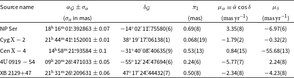
Gaia EDR3 counterparts with detected parallaxes
 $\pi_1$
for 4 PRE bursters and NP Ser
$\pi_1$
for 4 PRE bursters and NP Ser
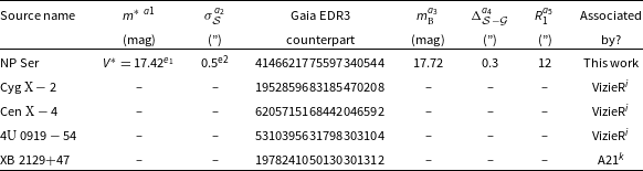
a1Apparent magnitude at a conventional passband;
a2positional uncertainty (adding in quadrature uncertainties in both directions) of the source (see Section 2);
a3apparent magnitude at the Gaia B band (Jordi et al. Reference Jordi2010), which covers the conventional G*, V*, B* bands and part of the R* band;
a4angular separation between the source and its Gaia counterpart, where
 $\alpha_\mathcal{G}$
and
$\alpha_\mathcal{G}$
and
 $\delta_\mathcal{G}$
were extrapolated to the respective epoch of
$\delta_\mathcal{G}$
were extrapolated to the respective epoch of
 $\alpha_\mathcal{S}$
(and
$\alpha_\mathcal{S}$
(and
 $\delta_{\mathcal{S}}$
) using the astrometric parameters in Table 2 (see Section 2 for more explanation);
$\delta_{\mathcal{S}}$
) using the astrometric parameters in Table 2 (see Section 2 for more explanation);
a5maximum search radius that contains only one Gaia source.
e1Deutsch et al. (1996);
e2Deutsch et al. (1999), where
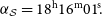 $\alpha_{\mathcal{S}}=18^{\textrm{h}}16^{\textrm{m}}01.^{\!\!{\textrm s}} $
380,
$\alpha_{\mathcal{S}}=18^{\textrm{h}}16^{\textrm{m}}01.^{\!\!{\textrm s}} $
380,
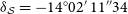 $\delta_{\mathcal{S}} = - 14^{\circ}02'\,11^{\prime\prime}34$
out of R-band CCD observation, with uncertainty radius of
$\delta_{\mathcal{S}} = - 14^{\circ}02'\,11^{\prime\prime}34$
out of R-band CCD observation, with uncertainty radius of
 $0^{\prime\prime}5$
at 90 confidence, measured at MJD 50674.
$0^{\prime\prime}5$
at 90 confidence, measured at MJD 50674.
 $^i$
Ochsenbein et al. (Reference Ochsenbein, Bauer and Marcout2000);
$^i$
Ochsenbein et al. (Reference Ochsenbein, Bauer and Marcout2000);
 $^k$
Arnason et al. (Reference Arnason, Papei, Barmby, Bahramian and Gorski2021).
$^k$
Arnason et al. (Reference Arnason, Papei, Barmby, Bahramian and Gorski2021).
Five astrometric parameters from Gaia EDR3 counterparts at year 2016.0 prior to calibration of Gaia parallaxes
In principle, the apparent magnitude of
 $\mathcal{G}$
should match that of the optical counterpart of
$\mathcal{G}$
should match that of the optical counterpart of
 $\mathcal{S}$
. However, making such a comparison is complicated by (1) the wide photometric passbands designed for the in-flight Gaia (Jordi et al. Reference Jordi2010) and (2) magnitude variability of stars.
$\mathcal{S}$
. However, making such a comparison is complicated by (1) the wide photometric passbands designed for the in-flight Gaia (Jordi et al. Reference Jordi2010) and (2) magnitude variability of stars.
On top of the 4 Gaia counterparts of PRE bursters (Cen
 $\textrm{X}-4$
, Cyg
$\textrm{X}-4$
, Cyg
 $\textrm{X}-2$
,
$\textrm{X}-2$
,
 $4\textrm{U}\,0919-54$
, and XB 2129+47) already recognised by VizieR and A21, we identified one Gaia counterpart with detected
$4\textrm{U}\,0919-54$
, and XB 2129+47) already recognised by VizieR and A21, we identified one Gaia counterpart with detected
 $\pi_1$
(from the remaining 12 objects), which was NP Ser (see Table 1). However, as we will discuss in Section 4.1, NP Ser is not the optical counterpart of GX
$\pi_1$
(from the remaining 12 objects), which was NP Ser (see Table 1). However, as we will discuss in Section 4.1, NP Ser is not the optical counterpart of GX
 $17+2$
, meaning that our final sample consists of 5 Gaia sources with detected
$17+2$
, meaning that our final sample consists of 5 Gaia sources with detected
 $\pi_1$
, of which 4 are PRE bursters.
$\pi_1$
, of which 4 are PRE bursters.
Hereafter, the 5 Gaia sources are sometimes referred to as ‘targets’. The (Gaia) B band covers the conventional
 $\textrm{G}^*$
,
$\textrm{G}^*$
,
 $\textrm{V}^*$
,
$\textrm{V}^*$
,
 $\textrm{B}^*$
bands and part of the
$\textrm{B}^*$
bands and part of the
 $\textrm{R}^*$
band. According to Table 1, the magnitude
$\textrm{R}^*$
band. According to Table 1, the magnitude
 $V^*$
of NP Ser measured at conventional
$V^*$
of NP Ser measured at conventional
 $\textrm{V}^*$
band generally agrees with
$\textrm{V}^*$
band generally agrees with
 $m_{\textrm{B}}$
of its Gaia counterpart. The 5 astrometric parameters of the Gaia counterparts for the 4 PRE bursters and NP Ser are summarised in Table 2.
$m_{\textrm{B}}$
of its Gaia counterpart. The 5 astrometric parameters of the Gaia counterparts for the 4 PRE bursters and NP Ser are summarised in Table 2.
3. Calibration of Gaia parallaxes
Before being applied for scientific purposes, each of the Gaia parallaxes
 $\pi_1$
needs to be calibrated by determining its (Gaia) parallax zero point
$\pi_1$
needs to be calibrated by determining its (Gaia) parallax zero point
 $\pi_0$
, as
$\pi_0$
, as
 $\pi_0$
has been shown to be systematically offset from zero (with an all-sky median of
$\pi_0$
has been shown to be systematically offset from zero (with an all-sky median of
 $-0.02$
mas for EDR3; Lindegren et al. Reference Lindegren2021b). Previous studies have revealed the dependence of
$-0.02$
mas for EDR3; Lindegren et al. Reference Lindegren2021b). Previous studies have revealed the dependence of
 $\pi_0$
on sky position, apparent magnitude, and colour (Lindegren et al. Reference Lindegren2018; Chen et al. Reference Chen, Richer, Caiazzo and Heyl2018; Huang et al. Reference Huang, Yuan, Beers and Zhang2021). Furthermore, Lindegren et al. (Reference Lindegren2021b) proposed that the position dependence of
$\pi_0$
on sky position, apparent magnitude, and colour (Lindegren et al. Reference Lindegren2018; Chen et al. Reference Chen, Richer, Caiazzo and Heyl2018; Huang et al. Reference Huang, Yuan, Beers and Zhang2021). Furthermore, Lindegren et al. (Reference Lindegren2021b) proposed that the position dependence of
 $\pi_0$
can be mostly attributed to the evolution of
$\pi_0$
can be mostly attributed to the evolution of
 $\pi_0$
with respect to ecliptic latitude
$\pi_0$
with respect to ecliptic latitude
 $\beta$
and derived an empirical global solution for five-parameter (see Lindegren et al. Reference Lindegren2021a for explanation) Gaia EDR3 sources and another such solution for six-parameter sources. While this approach is convenient to use, the empirical solutions do not provide an estimate of the uncertainty of
$\beta$
and derived an empirical global solution for five-parameter (see Lindegren et al. Reference Lindegren2021a for explanation) Gaia EDR3 sources and another such solution for six-parameter sources. While this approach is convenient to use, the empirical solutions do not provide an estimate of the uncertainty of
 $\pi_0$
and are only considered indicative (Lindegren et al. Reference Lindegren2021b).
$\pi_0$
and are only considered indicative (Lindegren et al. Reference Lindegren2021b).
In this work, we attempted a new pathway of generic
 $\pi_0$
determination. Unlike the global empirical solutions, the new
$\pi_0$
determination. Unlike the global empirical solutions, the new
 $\pi_0$
determination technique offers locally acquired
$\pi_0$
determination technique offers locally acquired
 $\pi_0$
and provides the uncertainty of the determined
$\pi_0$
and provides the uncertainty of the determined
 $\pi_0$
. We estimated
$\pi_0$
. We estimated
 $\pi_0$
for the 5 targets using a subset of the agn_cross_id table publicised along with EDR3 (Klioner et al. in preparation). We selected 1 592 629 quasar-like sources (out of the 1 614 173 sources in the agn_cross_id table), which (a) have
$\pi_0$
for the 5 targets using a subset of the agn_cross_id table publicised along with EDR3 (Klioner et al. in preparation). We selected 1 592 629 quasar-like sources (out of the 1 614 173 sources in the agn_cross_id table), which (a) have
 $m_{\textrm{B-R}}$
(denoted as ‘bp_rp’ in EDR3) values and (b) show no detected (
$m_{\textrm{B-R}}$
(denoted as ‘bp_rp’ in EDR3) values and (b) show no detected (
 $>\!3\,\sigma$
level) proper motion in either direction. Hereafter, we refer to this subset of 1 592 629 sources as the quasar catalog, and its sources as background quasars or quasars (when unambiguous).
$>\!3\,\sigma$
level) proper motion in either direction. Hereafter, we refer to this subset of 1 592 629 sources as the quasar catalog, and its sources as background quasars or quasars (when unambiguous).
On the sky, spatial patterns of
 $\pi_0$
on angular scales of up to
$\pi_0$
on angular scales of up to
 $\sim\!10^\circ$
are seen in Figure 2 of Lindegren et al. (Reference Lindegren2021b). We attempted different radius cuts (around each of the 5 targets) of up to
$\sim\!10^\circ$
are seen in Figure 2 of Lindegren et al. (Reference Lindegren2021b). We attempted different radius cuts (around each of the 5 targets) of up to
 $40^\circ$
, but found no clear evidence showing quasar parallaxes representative of the target
$40^\circ$
, but found no clear evidence showing quasar parallaxes representative of the target
 $\pi_0$
beyond a
$\pi_0$
beyond a
 $10^\circ$
radius cut. In most cases, a
$10^\circ$
radius cut. In most cases, a
 $10^\circ$
radius cut provides a sufficiently large sample of quasars for
$10^\circ$
radius cut provides a sufficiently large sample of quasars for
 $\pi_0$
estimation. Hence, we only present analysis of quasars within
$\pi_0$
estimation. Hence, we only present analysis of quasars within
 $10^\circ$
around each target.
$10^\circ$
around each target.
3.1. A new pathway to parallax zero points
Our
 $\pi_0$
determination is solely based on the quasar catalog (of 1 592 629 sources). The vital step of (Gaia) parallax calibration (or
$\pi_0$
determination is solely based on the quasar catalog (of 1 592 629 sources). The vital step of (Gaia) parallax calibration (or
 $\pi_0$
determination) is to select appropriate quasars in the same sky region with similar G-band apparent magnitudes
$\pi_0$
determination) is to select appropriate quasars in the same sky region with similar G-band apparent magnitudes
 $m_{\textrm{G}}$
and colours
$m_{\textrm{G}}$
and colours
 $m_{\textrm{B-R}}$
. We implemented this selection for each of the 5 targets by applying 4 filters to the quasar catalog: the angular-distance filter, the
$m_{\textrm{B-R}}$
. We implemented this selection for each of the 5 targets by applying 4 filters to the quasar catalog: the angular-distance filter, the
 $\beta$
filter, the
$\beta$
filter, the
 $m_{\textrm{G}}$
filter, and the
$m_{\textrm{G}}$
filter, and the
 $m_{\textrm{B-R}}$
filter. Once appropriate background quasars are chosen for each target, one can calculate
$m_{\textrm{B-R}}$
filter. Once appropriate background quasars are chosen for each target, one can calculate
 $\pi_0$
as the weighted mean parallax of this ‘sub-sample’, and the formal uncertainty of
$\pi_0$
as the weighted mean parallax of this ‘sub-sample’, and the formal uncertainty of
 $\pi_0$
.
$\pi_0$
.
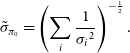 \begin{equation} \tilde{\sigma}_{\pi_0}=\left(\sum_{i}\frac{1}{{\sigma_i}^2}\right)^{-\frac{1}{2}}. \end{equation}
(Equation (4.19) in Bevington & Robinson Reference Bevington and Robinson2003), where
 $\sigma_i$
is the (Gaia) parallax error of each background quasar in the sub-sample.
$\sigma_i$
is the (Gaia) parallax error of each background quasar in the sub-sample.
We parameterised (1) the angular-distance filter using the search radius r around the target, (2) the
 $\beta$
filter using
$\beta$
filter using
 $\Delta \sin{\beta}$
, the half width of the
$\Delta \sin{\beta}$
, the half width of the
 $\sin{\beta}$
filter centred about
$\sin{\beta}$
filter centred about
 $\sin{\beta^\textrm{target}}$
, (3) the
$\sin{\beta^\textrm{target}}$
, (3) the
 $m_{\textrm{G}}$
filter using
$m_{\textrm{G}}$
filter using
 $\underline{\Delta} m_{\textrm{G}}$
, which stands for the relative half width (or
$\underline{\Delta} m_{\textrm{G}}$
, which stands for the relative half width (or
 $\Delta m_{\textrm{G}}/m_{\textrm{G}}^\textrm{target}$
) of the
$\Delta m_{\textrm{G}}/m_{\textrm{G}}^\textrm{target}$
) of the
 $m_{\textrm{G}}$
filter around
$m_{\textrm{G}}$
filter around
 $m_{\textrm{G}}^\textrm{target}$
, and (4) the
$m_{\textrm{G}}^\textrm{target}$
, and (4) the
 $m_{\textrm{B-R}}$
filter using
$m_{\textrm{B-R}}$
filter using
 $\Delta m_{\textrm{B-R}}$
, the half width of the
$\Delta m_{\textrm{B-R}}$
, the half width of the
 $m_{\textrm{B-R}}$
filter centred about
$m_{\textrm{B-R}}$
filter centred about
 $m_{\textrm{B-R}}^\textrm{target}$
.
$m_{\textrm{B-R}}^\textrm{target}$
.
Hence, the problem of
 $\pi_0$
determination using background quasars can be reduced to searching for optimal filter parameters (for each target), i.e. r,
$\pi_0$
determination using background quasars can be reduced to searching for optimal filter parameters (for each target), i.e. r,
 $\Delta \sin{\beta}$
,
$\Delta \sin{\beta}$
,
 $\underline{\Delta} m_{\textrm{G}}$
and
$\underline{\Delta} m_{\textrm{G}}$
and
 $\Delta m_{\textrm{B-R}}$
. For this search, we investigated the marginalised relation between
$\Delta m_{\textrm{B-R}}$
. For this search, we investigated the marginalised relation between
 $s_{\pi_0}^{*}$
and each of the 4 parameters (see the top 4-panel block of Figure 1), where
$s_{\pi_0}^{*}$
and each of the 4 parameters (see the top 4-panel block of Figure 1), where
 $s_{\pi_0}^{*}=s_{\pi_0}/s_{\pi_0}^\textrm{glb}$
stands for the weighted standard deviation of quasar parallaxes divided by its global value of 0.32 mas. To avoid small-sample fluctuations, Figure 1 starts at
$s_{\pi_0}^{*}=s_{\pi_0}/s_{\pi_0}^\textrm{glb}$
stands for the weighted standard deviation of quasar parallaxes divided by its global value of 0.32 mas. To avoid small-sample fluctuations, Figure 1 starts at
 $N_{\textrm{quasar}}=50$
, or
$N_{\textrm{quasar}}=50$
, or
 $N_{\textrm{quasar}}^\textrm{start}=50$
, which can also prevent overly small-sized sub-samples. To start with, we first introduce the
$N_{\textrm{quasar}}^\textrm{start}=50$
, which can also prevent overly small-sized sub-samples. To start with, we first introduce the
 $s_{\pi_0}^{*}$
-to-
$s_{\pi_0}^{*}$
-to-
 $\underline{\Delta} m_{\textrm{G}}$
relation and explain its implications. Relations between
$\underline{\Delta} m_{\textrm{G}}$
relation and explain its implications. Relations between
 $s_{\pi_0}^{*}$
and other 3 parameters can be interpreted in the same way.
$s_{\pi_0}^{*}$
and other 3 parameters can be interpreted in the same way.
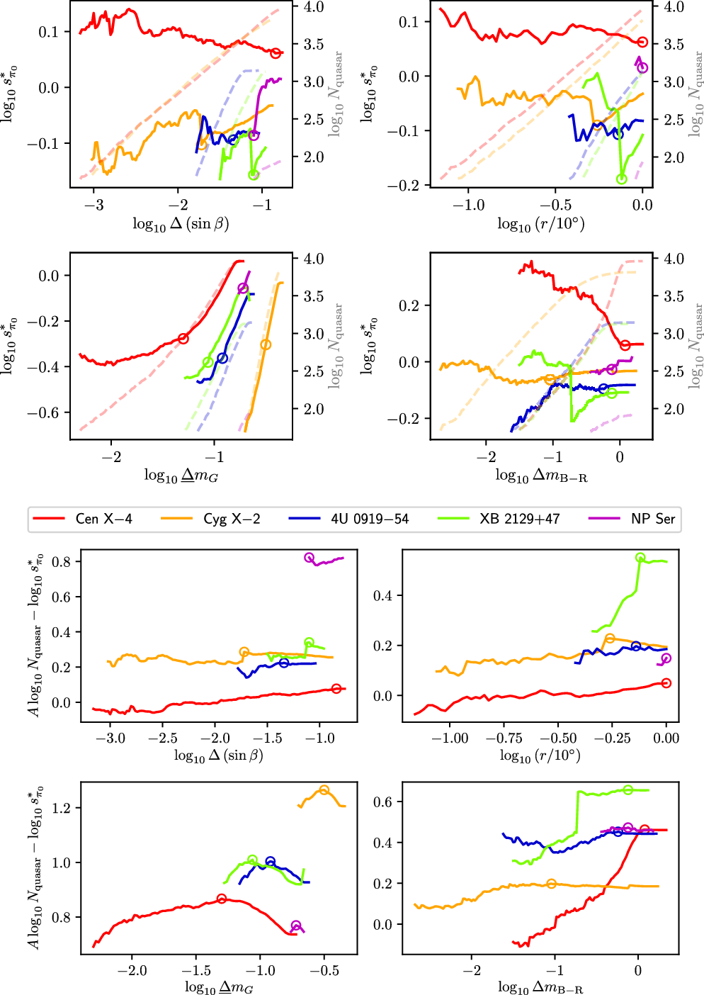
Top 4-panel block: The solid lines present the marginalised relations between
 $s_{\pi_0}^{*}$
of background quasars and 4 filter parameters:
$s_{\pi_0}^{*}$
of background quasars and 4 filter parameters:
 $\Delta \sin{\beta}$
(
$\Delta \sin{\beta}$
(
 $\beta$
denotes ecliptic latitude), search radius r around the target,
$\beta$
denotes ecliptic latitude), search radius r around the target,
 $\underline{\Delta} m_{\textrm{G}}$
and
$\underline{\Delta} m_{\textrm{G}}$
and
 $\Delta m_{\textrm{B-R}}$
. Here,
$\Delta m_{\textrm{B-R}}$
. Here,
 $s_{\pi_0}^{*}=s_{\pi_0}/s_{\pi_0}^{\textrm{glb}}$
, where
$s_{\pi_0}^{*}=s_{\pi_0}/s_{\pi_0}^{\textrm{glb}}$
, where
 $s_{\pi_0}$
and
$s_{\pi_0}$
and
 $s_{\pi_0}^{\textrm{glb}}$
represent the weighted standard deviation of quasar parallaxes and its global value (of the 1592629 quasars in the quasar catalog), respectively;
$s_{\pi_0}^{\textrm{glb}}$
represent the weighted standard deviation of quasar parallaxes and its global value (of the 1592629 quasars in the quasar catalog), respectively;
 $\Delta m_{\textrm{B-R}}$
|
$\Delta m_{\textrm{B-R}}$
|
 $\Delta \sin{\beta}$
stands for the half width of the
$\Delta \sin{\beta}$
stands for the half width of the
 $m_{\textrm{B-R}}$
|
$m_{\textrm{B-R}}$
|
 $\sin{\beta}$
filter centred around the
$\sin{\beta}$
filter centred around the
 $m_{\textrm{B-R}}^\textrm{target}$
|
$m_{\textrm{B-R}}^\textrm{target}$
|
 $\sin{\beta^\textrm{target}}$
(used to pick like-
$\sin{\beta^\textrm{target}}$
(used to pick like-
 $m_{\textrm{B-R}}$
|like-
$m_{\textrm{B-R}}$
|like-
 $\beta$
background quasars);
$\beta$
background quasars);
 $\underline{\Delta} m_{\textrm{G}}$
defines the half relative width of the
$\underline{\Delta} m_{\textrm{G}}$
defines the half relative width of the
 $m_{\textrm{G}}$
filter around
$m_{\textrm{G}}$
filter around
 $m_{\textrm{G}}^\textrm{target}$
used to select like-
$m_{\textrm{G}}^\textrm{target}$
used to select like-
 $m_{\textrm{G}}$
background quasars. The dashed curves lay out the marginalised relations between
$m_{\textrm{G}}$
background quasars. The dashed curves lay out the marginalised relations between
 $N_{\textrm{quasar}}$
and the 4 filter parameters, where
$N_{\textrm{quasar}}$
and the 4 filter parameters, where
 $N_{\textrm{quasar}}$
stands for number of remaining background quasars after being filtered. To avoid small-sample effect, the calculations start from
$N_{\textrm{quasar}}$
stands for number of remaining background quasars after being filtered. To avoid small-sample effect, the calculations start from
 $N_{\textrm{quasar}}=50$
, or
$N_{\textrm{quasar}}=50$
, or
 $N_{\textrm{quasar}}^{\textrm{start}}=50$
. The dependence of
$N_{\textrm{quasar}}^{\textrm{start}}=50$
. The dependence of
 $\pi_0$
on a variable (r,
$\pi_0$
on a variable (r,
 $\beta$
,
$\beta$
,
 $m_{\textrm{G}}$
, or
$m_{\textrm{G}}$
, or
 $m_{\textrm{B-R}}$
) is suggested if
$m_{\textrm{B-R}}$
) is suggested if
 $s_{\pi_0}^{*}$
grows with a larger filter (such as the
$s_{\pi_0}^{*}$
grows with a larger filter (such as the
 $m_{\textrm{G}}$
dependence), and vice versa. Bottom 4-panel block: The marginalised relation between the index
$m_{\textrm{G}}$
dependence), and vice versa. Bottom 4-panel block: The marginalised relation between the index
 $w=A \log_{10}N_{\textrm{quasar}}-\log_{10}s_{\pi_0}^{*}$
and each filter parameter, where
$w=A \log_{10}N_{\textrm{quasar}}-\log_{10}s_{\pi_0}^{*}$
and each filter parameter, where
 $A=(\log_{10}s_{\pi_0}^{*,max}-\log_{10}s_{\pi_0}^{*,min})/(\log_{10}N_{\textrm{quasar}}^{\max}-\log_{10}N_{\textrm{quasar}}^{\textrm{start}})$
is a scaling factor. The maximum of w is chosen (circled out in both bottom and top blocks) as the ‘optimal’ filter parameter.
$A=(\log_{10}s_{\pi_0}^{*,max}-\log_{10}s_{\pi_0}^{*,min})/(\log_{10}N_{\textrm{quasar}}^{\max}-\log_{10}N_{\textrm{quasar}}^{\textrm{start}})$
is a scaling factor. The maximum of w is chosen (circled out in both bottom and top blocks) as the ‘optimal’ filter parameter.
Unlike
 $\tilde{\sigma}_{\pi_0}$
, if a sufficiently large (
$\tilde{\sigma}_{\pi_0}$
, if a sufficiently large (
 $\gtrsim\!50$
) background-quasar sample had no
$\gtrsim\!50$
) background-quasar sample had no
 $m_{\textrm{G}}$
dependence (as opposed to Lindegren et al. Reference Lindegren2018; Lindegren et al. Reference Lindegren2021b),
$m_{\textrm{G}}$
dependence (as opposed to Lindegren et al. Reference Lindegren2018; Lindegren et al. Reference Lindegren2021b),
 $\log_{10} s_{\pi_0}^{*}$
would be expected to be largely independent to
$\log_{10} s_{\pi_0}^{*}$
would be expected to be largely independent to
 $\underline{\Delta} m_{\textrm{G}}$
, and to fluctuate around the global value 0. This is clearly not the case for all of the 5 targets. From Figure 1, we found an obvious upward trend of
$\underline{\Delta} m_{\textrm{G}}$
, and to fluctuate around the global value 0. This is clearly not the case for all of the 5 targets. From Figure 1, we found an obvious upward trend of
 $s_{\pi_0}^{*}$
with growing
$s_{\pi_0}^{*}$
with growing
 $\underline{\Delta} m_{\textrm{G}}$
. This upward trend shows that background quasars with similar
$\underline{\Delta} m_{\textrm{G}}$
. This upward trend shows that background quasars with similar
 $m_{\textrm{G}}$
around
$m_{\textrm{G}}$
around
 $m_{\textrm{G}}^\textrm{target}$
tend to have similar parallaxes, which supports the
$m_{\textrm{G}}^\textrm{target}$
tend to have similar parallaxes, which supports the
 $m_{\textrm{G}}$
-dependence of
$m_{\textrm{G}}$
-dependence of
 $\pi_0$
stated in Lindegren et al. (Reference Lindegren2018); Lindegren et al. (Reference Lindegren2021b).
$\pi_0$
stated in Lindegren et al. (Reference Lindegren2018); Lindegren et al. (Reference Lindegren2021b).
Using the same interpretation, we also investigated marginalised relations of
 $s_{\pi_0}^{*}$
with respect to each of the other 3 filter parameters. As can be seen in Figure 1, most fields show a (weak) colour dependence of
$s_{\pi_0}^{*}$
with respect to each of the other 3 filter parameters. As can be seen in Figure 1, most fields show a (weak) colour dependence of
 $\pi_0$
. For the two sky-position-related filter parameters,
$\pi_0$
. For the two sky-position-related filter parameters,
 $\beta$
dependence of
$\beta$
dependence of
 $\pi_0$
is clearly found in the target fields of Cyg
$\pi_0$
is clearly found in the target fields of Cyg
 $\textrm{X}-2$
and NP Ser, whereas the r dependence of
$\textrm{X}-2$
and NP Ser, whereas the r dependence of
 $\pi_0$
is hardly noticeable in any of the 5 target fields. This contrast reinforces the belief that the
$\pi_0$
is hardly noticeable in any of the 5 target fields. This contrast reinforces the belief that the
 $\beta$
dependence of
$\beta$
dependence of
 $\pi_0$
contributes considerably to the position dependence of
$\pi_0$
contributes considerably to the position dependence of
 $\pi_0$
(Lindegren et al. Reference Lindegren2021b). Additionally,
$\pi_0$
(Lindegren et al. Reference Lindegren2021b). Additionally,
 $\log_{10} s_{\pi_0}^{*}$
converges to
$\log_{10} s_{\pi_0}^{*}$
converges to
 $0.0\pm0.1$
at
$0.0\pm0.1$
at
 $r=10^\circ$
in all target fields, which roughly agrees with our assumption that the r-dependence of
$r=10^\circ$
in all target fields, which roughly agrees with our assumption that the r-dependence of
 $\pi_0$
becomes negligible beyond
$\pi_0$
becomes negligible beyond
 $10^\circ$
search radius; in other words, quasar parallaxes at
$10^\circ$
search radius; in other words, quasar parallaxes at
 $r>10^\circ$
are almost not representative of the target
$r>10^\circ$
are almost not representative of the target
 $\pi_0$
.
$\pi_0$
.
Knowing the way to interpret the relation between
 $s_{\pi_0}^{*}$
and each of the filter parameters, we can proceed to choose the optimal filter parameters. In choosing filter parameters, one wants the filtered sub-sample to have a consistently low level of
$s_{\pi_0}^{*}$
and each of the filter parameters, we can proceed to choose the optimal filter parameters. In choosing filter parameters, one wants the filtered sub-sample to have a consistently low level of
 $s_{\pi_0}^{*}$
; meanwhile, one prefers a filtered sub-sample as large as possible to achieve reliable and precise
$s_{\pi_0}^{*}$
; meanwhile, one prefers a filtered sub-sample as large as possible to achieve reliable and precise
 $\pi_0$
. To meet both demands is difficult when
$\pi_0$
. To meet both demands is difficult when
 $s_{\pi_0}^{*}$
rises with a larger filter (as is the case for the
$s_{\pi_0}^{*}$
rises with a larger filter (as is the case for the
 $m_{\textrm{G}}$
filter). In this regard, we created an index
$m_{\textrm{G}}$
filter). In this regard, we created an index
 $w=A \log_{10} N_{\textrm{quasar}} - \log_{10} s_{\pi_0}^{*}$
, where
$w=A \log_{10} N_{\textrm{quasar}} - \log_{10} s_{\pi_0}^{*}$
, where
 $A=(\log_{10}s_{\pi_0}^{*,\max}-\log_{10}s_{\pi_0}^{*,\min})/(\log_{10}N_{\textrm{quasar}}^{\max}-\log_{10}N_{\textrm{quasar}}^{\textrm{start}})$
is a scaling factor. Instead of the minimum of
$A=(\log_{10}s_{\pi_0}^{*,\max}-\log_{10}s_{\pi_0}^{*,\min})/(\log_{10}N_{\textrm{quasar}}^{\max}-\log_{10}N_{\textrm{quasar}}^{\textrm{start}})$
is a scaling factor. Instead of the minimum of
 $s_{\pi_0}^{*}$
or the maximum of
$s_{\pi_0}^{*}$
or the maximum of
 $N_{\textrm{quasar}}$
, we adopted the filter parameter at the peak of the index w (see the bottom 4-panel block of Figure 1), so that an optimised trade-off between
$N_{\textrm{quasar}}$
, we adopted the filter parameter at the peak of the index w (see the bottom 4-panel block of Figure 1), so that an optimised trade-off between
 $s_{\pi_0}^{*}$
and
$s_{\pi_0}^{*}$
and
 $N_{\textrm{quasar}}$
can be reached. Using this consistent standard, we reached the parameter of each filter for each target (see Table 3).
$N_{\textrm{quasar}}$
can be reached. Using this consistent standard, we reached the parameter of each filter for each target (see Table 3).
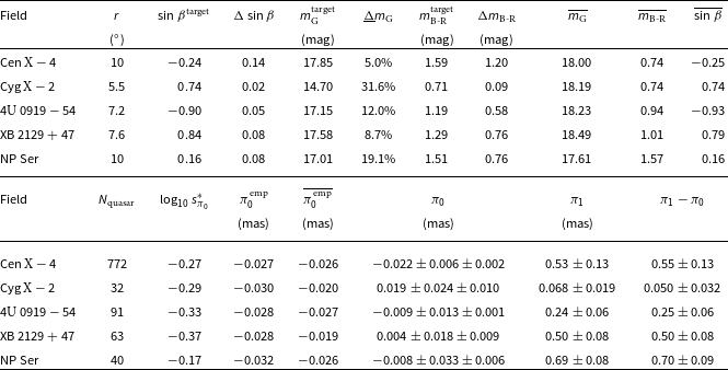
The information of the 4 filters (including search radius r,
 $\beta$
filter,
$\beta$
filter,
 $m_{\textrm{G}}$
filter, and
$m_{\textrm{G}}$
filter, and
 $m_{\textrm{B-R}}$
filter, see Section 3.1 for explanation) and the parallax zero point
$m_{\textrm{B-R}}$
filter, see Section 3.1 for explanation) and the parallax zero point
 $\pi_0$
calculated from the respective sub-sample of background quasars after applying the 4 filters.
$\pi_0$
calculated from the respective sub-sample of background quasars after applying the 4 filters.
 $\pi_1$
and
$\pi_1$
and
 $\pi_1-\pi_0$
stand for uncalibrated parallaxes and calibrated parallaxes, respectively.
$\pi_1-\pi_0$
stand for uncalibrated parallaxes and calibrated parallaxes, respectively.
 $\overline{m_{\textrm{G}}}$
,
$\overline{m_{\textrm{G}}}$
,
 $\overline{m_{\textrm{B-R}}}$
, and
$\overline{m_{\textrm{B-R}}}$
, and
 $\overline{\sin{\beta}}$
represent the respective weighted average value of the three filter parameters (see Section 3.1).
$\overline{\sin{\beta}}$
represent the respective weighted average value of the three filter parameters (see Section 3.1).
 $N_{\textrm{quasar}}$
and
$N_{\textrm{quasar}}$
and
 $s_{\pi_0}^{*}$
(defined in Section 3.1) are reported for the filtered quasar sub-sample in each target field. The empirical parallax zero-point solutions for the targets calculated with zero_point.zpt (https://gitlab.com/icc-ub/public/gaiadr3_zeropoint) are provided as
$s_{\pi_0}^{*}$
(defined in Section 3.1) are reported for the filtered quasar sub-sample in each target field. The empirical parallax zero-point solutions for the targets calculated with zero_point.zpt (https://gitlab.com/icc-ub/public/gaiadr3_zeropoint) are provided as
 $\pi_0^\textrm{emp}$
. The weighted average empirical parallax zero points of the sub-samples (see Section 3.1) are presented as
$\pi_0^\textrm{emp}$
. The weighted average empirical parallax zero points of the sub-samples (see Section 3.1) are presented as
 $\overline{\pi_0^\textrm{emp}}$
After applying the 4 filters, we acquired a quasar sub-sample of
 $N_{\textrm{quasar}}$
and
$N_{\textrm{quasar}}$
and
 $s_{\pi_0}^{*}$
for each target and obtained
$s_{\pi_0}^{*}$
for each target and obtained
 $\pi_0$
of the target from this sub-sample (see Table 3). Due to the relative paucity of quasars identified at low Galactic latitudes b (for the reasons discussed in Lindegren et al. Reference Lindegren2021b), NP Ser,
$\pi_0$
of the target from this sub-sample (see Table 3). Due to the relative paucity of quasars identified at low Galactic latitudes b (for the reasons discussed in Lindegren et al. Reference Lindegren2021b), NP Ser,
 $4\textrm{U}\,0919-54$
, and XB 2129+47 (all of which have
$4\textrm{U}\,0919-54$
, and XB 2129+47 (all of which have
 $|b|<4^\circ$
) receive relatively low values for
$|b|<4^\circ$
) receive relatively low values for
 $N_{\textrm{quasar}}$
compared to Cen
$N_{\textrm{quasar}}$
compared to Cen
 $\textrm{X}-4$
(
$\textrm{X}-4$
(
 $b=24^\circ$
), which partly lead to the relatively large
$b=24^\circ$
), which partly lead to the relatively large
 $\tilde{\sigma}_{\pi_0}$
. Nonetheless, we have shown that
$\tilde{\sigma}_{\pi_0}$
. Nonetheless, we have shown that
 $\pi_0$
for targets at
$\pi_0$
for targets at
 $|b|<6^\circ$
can be determined with nearby (on the sky) quasars. On the other hand, Cyg
$|b|<6^\circ$
can be determined with nearby (on the sky) quasars. On the other hand, Cyg
 $\textrm{X}-2$
, despite being located at
$\textrm{X}-2$
, despite being located at
 $b=-11^\circ$
, has the smallest
$b=-11^\circ$
, has the smallest
 $N_{\textrm{quasar}}$
and the largest
$N_{\textrm{quasar}}$
and the largest
 $\tilde{\sigma}_{\pi_0}$
among the 5 targets. This is mainly due to the relative rarity of bright quasars (Cyg
$\tilde{\sigma}_{\pi_0}$
among the 5 targets. This is mainly due to the relative rarity of bright quasars (Cyg
 $\textrm{X}-2$
has
$\textrm{X}-2$
has
 $m_{\textrm{G}}=14.7$
mag).
$m_{\textrm{G}}=14.7$
mag).
The negative
 $\log_{10} s_{\pi_0}^{*}$
of the quasar sub-sample for each target indicates that the sub-sample of (closely located, like-
$\log_{10} s_{\pi_0}^{*}$
of the quasar sub-sample for each target indicates that the sub-sample of (closely located, like-
 $\beta$
, like-
$\beta$
, like-
 $m_{\textrm{G}}$
, and like-
$m_{\textrm{G}}$
, and like-
 $m_{\textrm{B-R}}$
) quasars is representative of the target source. Despite this good representativeness, the
$m_{\textrm{B-R}}$
) quasars is representative of the target source. Despite this good representativeness, the
 $\tilde{\sigma}_{\pi_0}$
estimated with Equation (2) is still an under-estimate for the uncertainty of
$\tilde{\sigma}_{\pi_0}$
estimated with Equation (2) is still an under-estimate for the uncertainty of
 $\pi_0$
, as the sub-sample has a spread in each parameter and does not represent the target perfectly. We estimated the weighted average
$\pi_0$
, as the sub-sample has a spread in each parameter and does not represent the target perfectly. We estimated the weighted average
 $m_{\textrm{G}}$
,
$m_{\textrm{G}}$
,
 $m_{\textrm{B-R}}$
, and
$m_{\textrm{B-R}}$
, and
 $\sin{\beta}$
of the quasar sub-sample (where the weighting is
$\sin{\beta}$
of the quasar sub-sample (where the weighting is
 $1/{\sigma_i}^2$
, see Equation (2) for the definition of
$1/{\sigma_i}^2$
, see Equation (2) for the definition of
 $\sigma_i$
), which are presented in Table 3 as
$\sigma_i$
), which are presented in Table 3 as
 $\overline{m_{\textrm{G}}}$
,
$\overline{m_{\textrm{G}}}$
,
 $\overline{m_{\textrm{B-R}}}$
, and
$\overline{m_{\textrm{B-R}}}$
, and
 $\overline{\sin{\beta}}$
, respectively. According to Table 3, there are residual offsets of
$\overline{\sin{\beta}}$
, respectively. According to Table 3, there are residual offsets of
 $\sin{\beta}$
,
$\sin{\beta}$
,
 $m_{\textrm{G}}$
, and
$m_{\textrm{G}}$
, and
 $m_{\textrm{B-R}}$
between the target and the average level of the sub-sample, which would result in extra systematic error for the
$m_{\textrm{B-R}}$
between the target and the average level of the sub-sample, which would result in extra systematic error for the
 $\pi_0$
estimates. To estimate this systematic error of
$\pi_0$
estimates. To estimate this systematic error of
 $\pi_0$
, we calculated the empirical parallax zero points for the targets (see Table 3) using zero_point.zpt (https://gitlab.com/icc-ub/public/gaiadr3_zeropoint, Lindegren et al. Reference Lindegren2021b), noted as
$\pi_0$
, we calculated the empirical parallax zero points for the targets (see Table 3) using zero_point.zpt (https://gitlab.com/icc-ub/public/gaiadr3_zeropoint, Lindegren et al. Reference Lindegren2021b), noted as
 $\pi_0^\textrm{emp}$
. In the same way, we also estimated the empirical parallax zero points for each quasar of the sub-sample, then derived the weighted average empirical parallax zero point of the sub-sample, noted as
$\pi_0^\textrm{emp}$
. In the same way, we also estimated the empirical parallax zero points for each quasar of the sub-sample, then derived the weighted average empirical parallax zero point of the sub-sample, noted as
 $\overline{\pi_0^\textrm{emp}}$
(see Table 3). The difference between
$\overline{\pi_0^\textrm{emp}}$
(see Table 3). The difference between
 $\pi_0^\textrm{emp}$
and
$\pi_0^\textrm{emp}$
and
 $\overline{\pi_0^\textrm{emp}}$
is taken as an estimate for the systematic error of
$\overline{\pi_0^\textrm{emp}}$
is taken as an estimate for the systematic error of
 $\pi_0$
, which is added in quadrature to the
$\pi_0$
, which is added in quadrature to the
 $\tilde{\sigma}_{\pi_0}$
calculated with Equation (2).
$\tilde{\sigma}_{\pi_0}$
calculated with Equation (2).
No uncertainties are yet available for
 $\pi_0^\textrm{emp}$
. Regardless, all of our
$\pi_0^\textrm{emp}$
. Regardless, all of our
 $\pi_0$
are consistent with the empirical counterparts at the
$\pi_0$
are consistent with the empirical counterparts at the
 $2\,\sigma$
confidence level. We note that
$2\,\sigma$
confidence level. We note that
 $\pi_0^\textrm{emp}$
is only used to estimate the systematic error of
$\pi_0^\textrm{emp}$
is only used to estimate the systematic error of
 $\pi_0$
and is not adopted in the discussions that follow. The calibrated parallaxes
$\pi_0$
and is not adopted in the discussions that follow. The calibrated parallaxes
 $\pi_1-\pi_0$
are summarised in Table 3.
$\pi_1-\pi_0$
are summarised in Table 3.
Despite the overall consistency between
 $\pi_0$
and
$\pi_0$
and
 $\pi_0^\textrm{emp}$
, it is noteworthy that all
$\pi_0^\textrm{emp}$
, it is noteworthy that all
 $\pi_0$
are larger than the
$\pi_0$
are larger than the
 $\pi_0^\textrm{emp}$
counterparts, which can be a coincidence of small-number statistics. Alternatively, knowing that most of the targets are situated at low b, it might indicate a systematic offset between quasar-sub-sample-based
$\pi_0^\textrm{emp}$
counterparts, which can be a coincidence of small-number statistics. Alternatively, knowing that most of the targets are situated at low b, it might indicate a systematic offset between quasar-sub-sample-based
 $\pi_0$
and
$\pi_0$
and
 $\pi_0^\textrm{emp}$
at low b. Interestingly, a recent parallax zero-point study based on
$\pi_0^\textrm{emp}$
at low b. Interestingly, a recent parallax zero-point study based on
 $\sim$
110 000 W Ursae Majoris variables showed that the W-Ursae-Majoris-variable-based
$\sim$
110 000 W Ursae Majoris variables showed that the W-Ursae-Majoris-variable-based
 $\pi_0$
are systematically larger than the
$\pi_0$
are systematically larger than the
 $\pi_0^\textrm{emp}$
counterparts at low b (see Figure 3 of Ren et al. Reference Ren, Chen, Zhang, de Grijs, Deng and Huang2021). Hence, a future quasar-sub-sample-based study involving a large sample of targets (and other parallax zero-point studies by different approaches) will be essential for probing
$\pi_0^\textrm{emp}$
counterparts at low b (see Figure 3 of Ren et al. Reference Ren, Chen, Zhang, de Grijs, Deng and Huang2021). Hence, a future quasar-sub-sample-based study involving a large sample of targets (and other parallax zero-point studies by different approaches) will be essential for probing
 $\pi_0^\textrm{emp}$
at low b. More specifically, if quasar-sub-sample-based
$\pi_0^\textrm{emp}$
at low b. More specifically, if quasar-sub-sample-based
 $\pi_0$
at low b are confirmed to be systematically larger than the
$\pi_0$
at low b are confirmed to be systematically larger than the
 $\pi_0^\textrm{emp}$
counterparts, then it is likely that
$\pi_0^\textrm{emp}$
counterparts, then it is likely that
 $\pi_0^\textrm{emp}$
is systematically under-estimated at low b.
$\pi_0^\textrm{emp}$
is systematically under-estimated at low b.
4. Discussion
In this section, we discuss the implications of the 5 calibrated parallaxes
 $\pi_1-\pi_0$
provided in Table 3.
$\pi_1-\pi_0$
provided in Table 3.
4.1. NP Ser and GX
$17+2$
revisited

GX
 $17+2$
is one of the brightest X-ray sources on the sky, from which 43 PRE bursts have been recorded (see Table 1 of Galloway et al. Reference Galloway2020 and references therein); its distance was estimated to be 7.3–12.6 kpc by treating its PRE bursts as standard candles (as explained in Section 1), where the distance uncertainty is dominated by the uncertain composition of the nuclear fuel (Galloway et al. Reference Galloway2020). The optical source NP Ser,
$17+2$
is one of the brightest X-ray sources on the sky, from which 43 PRE bursts have been recorded (see Table 1 of Galloway et al. Reference Galloway2020 and references therein); its distance was estimated to be 7.3–12.6 kpc by treating its PRE bursts as standard candles (as explained in Section 1), where the distance uncertainty is dominated by the uncertain composition of the nuclear fuel (Galloway et al. Reference Galloway2020). The optical source NP Ser,
 $\approx1.^{\prime\prime}0$
away from GX
$\approx1.^{\prime\prime}0$
away from GX
 $17+2$
, was initially considered the optical counterpart of GX
$17+2$
, was initially considered the optical counterpart of GX
 $17+2$
(Tarenghi & Reina Reference Tarenghi and Reina1972), but the association has been ruled out, based on its sky-position offset from GX
$17+2$
(Tarenghi & Reina Reference Tarenghi and Reina1972), but the association has been ruled out, based on its sky-position offset from GX
 $17+2$
(Deutsch et al. Reference Deutsch, Margon, Anderson, Wachter and Goss1999) and its lack of optical variability (as expected for the optical counterpart of GX
$17+2$
(Deutsch et al. Reference Deutsch, Margon, Anderson, Wachter and Goss1999) and its lack of optical variability (as expected for the optical counterpart of GX
 $17+2$
) (e.g. Davidsen et al. Reference Davidsen, Malina and Bowyer1976; Margon Reference Margon1978). Despite this, NP Ser was initially treated as a potential counterpart and the Gaia properties of NP Ser were analysed. Regardless of the non-association of NP Ser and GX
$17+2$
) (e.g. Davidsen et al. Reference Davidsen, Malina and Bowyer1976; Margon Reference Margon1978). Despite this, NP Ser was initially treated as a potential counterpart and the Gaia properties of NP Ser were analysed. Regardless of the non-association of NP Ser and GX
 $17+2$
, the complex sky region around GX
$17+2$
, the complex sky region around GX
 $17+2$
for optical/infrared observations (see Figure 2 of Deutsch et al. Reference Deutsch, Margon, Anderson, Wachter and Goss1999 for example) merits high-precision Gaia astrometry of NP Ser, which will facilitate future data analysis of optical/infrared observations of GX
$17+2$
for optical/infrared observations (see Figure 2 of Deutsch et al. Reference Deutsch, Margon, Anderson, Wachter and Goss1999 for example) merits high-precision Gaia astrometry of NP Ser, which will facilitate future data analysis of optical/infrared observations of GX
 $17+2$
.
$17+2$
.
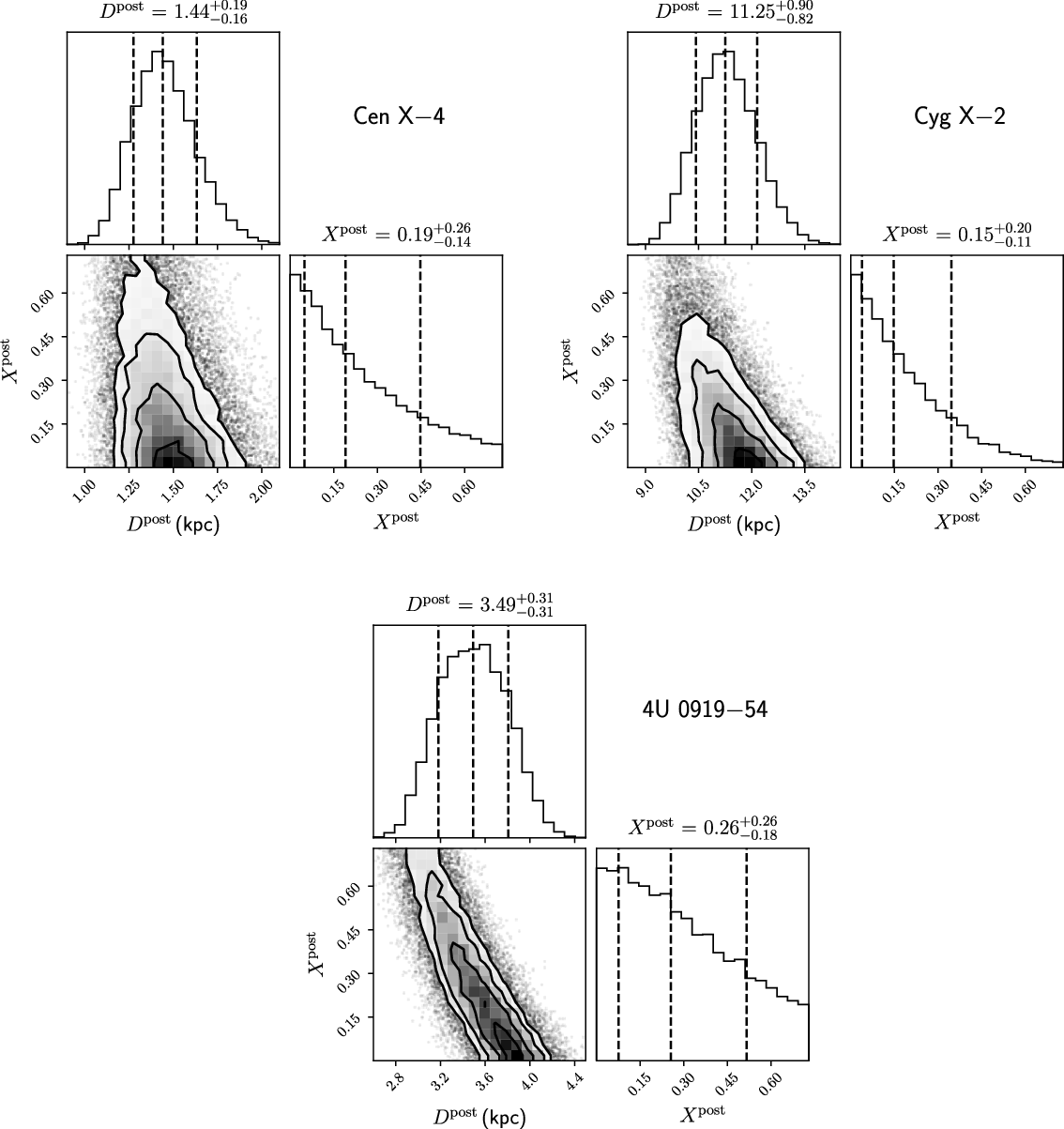
2-D histograms and marginalised 1-D histograms for posterior distance
 $D^{\textrm{post}}$
and posterior mass fraction of hydrogen of nuclear fuel
$D^{\textrm{post}}$
and posterior mass fraction of hydrogen of nuclear fuel
 $X^{\textrm{post}}$
simulated with bilby (Ashton et al. Reference Ashton2019) and plotted with corner.py (Foreman-Mackey Reference Foreman-Mackey2016). The n-th contour in each 2-D histogram contains
$X^{\textrm{post}}$
simulated with bilby (Ashton et al. Reference Ashton2019) and plotted with corner.py (Foreman-Mackey Reference Foreman-Mackey2016). The n-th contour in each 2-D histogram contains
 $1-\exp\left(-n^2/2\right)$
of the simulated sample (Foreman-Mackey Reference Foreman-Mackey2016). The vertical lines in the middle and two sides mark the median and central 68% of the sample, respectively.
$1-\exp\left(-n^2/2\right)$
of the simulated sample (Foreman-Mackey Reference Foreman-Mackey2016). The vertical lines in the middle and two sides mark the median and central 68% of the sample, respectively.
Using the astrometric parameters of NP Ser in Tables 2 and 3, we extrapolated the reference position of NP Ser (from the reference epoch 2016.0 yr, or MJD 57388) to MJD 47496, following the method described in Section 3.2 of Ding et al. (Reference Ding, Deller, Freire, Kaplan, Lazio, Shannon and Stappers2020). The projected Gaia position of NP Ser is offset from the VLA position of GX
 $17+2$
(see Table 2 of Deutsch et al. Reference Deutsch, Margon, Anderson, Wachter and Goss1999) by
$17+2$
(see Table 2 of Deutsch et al. Reference Deutsch, Margon, Anderson, Wachter and Goss1999) by
 $0.^{\!\prime\prime}95\pm0.^{\!\prime\prime}07$
at MJD 47496. Considering the distances to GX
$0.^{\!\prime\prime}95\pm0.^{\!\prime\prime}07$
at MJD 47496. Considering the distances to GX
 $17+2$
and NP Ser, nuclear fuel with cosmic abundances (73% hydrogen) corresponds to the smallest PRE distance of
$17+2$
and NP Ser, nuclear fuel with cosmic abundances (73% hydrogen) corresponds to the smallest PRE distance of
 $8.5\pm1.2$
kpc for GX
$8.5\pm1.2$
kpc for GX
 $17+2$
(Galloway et al. Reference Galloway2020); in comparison, the calibrated Gaia parallax of NP Ser is
$17+2$
(Galloway et al. Reference Galloway2020); in comparison, the calibrated Gaia parallax of NP Ser is
 $0.70\pm0.09$
mas, corresponding to a distance of
$0.70\pm0.09$
mas, corresponding to a distance of
 $1.44^{+0.21}_{-0.16}$
kpc, which establishes NP Ser as a foreground source of GX
$1.44^{+0.21}_{-0.16}$
kpc, which establishes NP Ser as a foreground source of GX
 $17+2$
. The current sky-position offset between NP Ser and GX
$17+2$
. The current sky-position offset between NP Ser and GX
 $17+2$
depends on the proper motion of GX
$17+2$
depends on the proper motion of GX
 $17+2$
. Assuming GX
$17+2$
. Assuming GX
 $17+2$
rotates around the Galactic centre in the Galactic disk with negligible peculiar velocity (with respect to the neighbourhood of GX
$17+2$
rotates around the Galactic centre in the Galactic disk with negligible peculiar velocity (with respect to the neighbourhood of GX
 $17+2$
), the apparent proper motion of GX
$17+2$
), the apparent proper motion of GX
 $17+2$
would be
$17+2$
would be
 $\mu_{\alpha}=-3.5$
 $\textrm{mas yr}^{-1}$
and
$\textrm{mas yr}^{-1}$
and
 $\mu_{\delta}=-6.7$
 $\textrm{mas yr}^{-1}$
given a distance of 8.5 kpc (from the Earth). Based on this indicative proper motion of GX
$\textrm{mas yr}^{-1}$
given a distance of 8.5 kpc (from the Earth). Based on this indicative proper motion of GX
 $17+2$
and the Gaia ephemeris of NP Ser, NP Ser is currently (at MJD 59394)
$17+2$
and the Gaia ephemeris of NP Ser, NP Ser is currently (at MJD 59394)
 $1.^{\prime\prime}0$
away from GX
$1.^{\prime\prime}0$
away from GX
 $17+2$
and continues to move away from GX
$17+2$
and continues to move away from GX
 $17+2$
on the sky; accordingly, it would become easier with time to resolve GX
$17+2$
on the sky; accordingly, it would become easier with time to resolve GX
 $17+2$
from the foreground NP Ser in optical/infrared observations.
$17+2$
from the foreground NP Ser in optical/infrared observations.
4.2. Posterior distances and compositions of nuclear fuel for Cen
$\textrm{X}-4$
, Cyg
$\textrm{X}-2$
, and
$4\textrm{U}\,0919-54$


Among the (calibrated) parallaxes
 $\pi_1-\pi_0$
of the 4 PRE bursters (i.e. Cen
$\pi_1-\pi_0$
of the 4 PRE bursters (i.e. Cen
 $\textrm{X}-4$
, Cyg
$\textrm{X}-4$
, Cyg
 $\textrm{X}-2$
,
$\textrm{X}-2$
,
 $4\textrm{U}\,0919-54$
, and XB 2129+47),
$4\textrm{U}\,0919-54$
, and XB 2129+47),
 $\pi_1-\pi_0$
for Cen
$\pi_1-\pi_0$
for Cen
 $\textrm{X}-4$
,
$\textrm{X}-4$
,
 $4\textrm{U}\,0919-54$
and XB 2129+47 are detected, whereas
$4\textrm{U}\,0919-54$
and XB 2129+47 are detected, whereas
 $\pi_1-\pi_0$
of Cyg
$\pi_1-\pi_0$
of Cyg
 $\textrm{X}-2$
is weakly constrained. All PRE bursters except XB 2129+47 have nominal PRE distances published that are inferred from their respective PRE bursts (see Table 4 for PRE distances and their references). Using Bayesian inference, we can incorporate the parallax of a PRE burster with its nominal PRE distance to constrain the composition of nuclear fuel and refine the nominal PRE distance.
$\textrm{X}-2$
is weakly constrained. All PRE bursters except XB 2129+47 have nominal PRE distances published that are inferred from their respective PRE bursts (see Table 4 for PRE distances and their references). Using Bayesian inference, we can incorporate the parallax of a PRE burster with its nominal PRE distance to constrain the composition of nuclear fuel and refine the nominal PRE distance.
In Section 1, we have mentioned that the Eddington luminosity (measured by an observer at infinity)
 $L_{\textrm{Edd},\infty}$
varies with NS mass
$L_{\textrm{Edd},\infty}$
varies with NS mass
 $M_{\textrm{NS}}$
and photosphere radius
$M_{\textrm{NS}}$
and photosphere radius
 $R_{\textrm{P}}$
(see Equation (1)). In practice, the bolometric flux at the ‘touchdown’ (when the photosphere drops back to the NS surface) of a PRE burst is compared to the theoretical
$R_{\textrm{P}}$
(see Equation (1)). In practice, the bolometric flux at the ‘touchdown’ (when the photosphere drops back to the NS surface) of a PRE burst is compared to the theoretical
 $L_{\textrm{Edd},\infty}$
at
$L_{\textrm{Edd},\infty}$
at
 $R_{\textrm{P}}=R_{\textrm{NS}}$
(where
$R_{\textrm{P}}=R_{\textrm{NS}}$
(where
 $R_{\textrm{NS}}$
stands for NS radius) to calculate the nominal PRE distance (Galloway et al. Reference Galloway2020). Therefore, the theoretical
$R_{\textrm{NS}}$
stands for NS radius) to calculate the nominal PRE distance (Galloway et al. Reference Galloway2020). Therefore, the theoretical
 $L_{\textrm{Edd},\infty}$
should change with
$L_{\textrm{Edd},\infty}$
should change with
 $M_{\textrm{NS}}$
and
$M_{\textrm{NS}}$
and
 $R_{\textrm{NS}}$
, which is, however, not taken into account in this work. We note that, following Galloway et al. (Reference Galloway2020), we assume
$R_{\textrm{NS}}$
, which is, however, not taken into account in this work. We note that, following Galloway et al. (Reference Galloway2020), we assume
 $M_{\textrm{NS}}=1.4\,\textrm{M}_{\odot}$
and
$M_{\textrm{NS}}=1.4\,\textrm{M}_{\odot}$
and
 $R_{\textrm{NS}}=11.2$
km (Steiner et al. Reference Steiner, Heinke, Bogdanov, Li, Ho, Bahramian and Han2018) for all PRE bursters.
$R_{\textrm{NS}}=11.2$
km (Steiner et al. Reference Steiner, Heinke, Bogdanov, Li, Ho, Bahramian and Han2018) for all PRE bursters.
4.2.1. Bayes factor between two ends of the composition of nuclear fuel
As mentioned in Section 1, the Eddington luminosity of PRE bursts depends on the composition of nuclear fuel (accreted onto the NS surface from its companion) at the time of the outburst. This composition is normally parameterised by X, the mass fraction of hydrogen in nuclear fuel at the time of a PRE burst, which generally ranges from 0 to
 $\approx73$
%, the cosmic mass fraction of hydrogen. As the result of the dynamic nucleosynthesis process during accretion, X varies from one PRE burst to another, but is always smaller than the hydrogen mass fraction of the donor star. X can be roughly predicted by the theoretical ignition models of X-ray bursts and mainly depends on the local accretion rate
$\approx73$
%, the cosmic mass fraction of hydrogen. As the result of the dynamic nucleosynthesis process during accretion, X varies from one PRE burst to another, but is always smaller than the hydrogen mass fraction of the donor star. X can be roughly predicted by the theoretical ignition models of X-ray bursts and mainly depends on the local accretion rate
 $\dot{m}$
(e.g. Fujimoto, Hanawa, & Miyaji, Reference Fujimoto, Hanawa and Miyaji1981).
$\dot{m}$
(e.g. Fujimoto, Hanawa, & Miyaji, Reference Fujimoto, Hanawa and Miyaji1981).
Nominal PRE distances for
 $X=0$
, denoted as
$X=0$
, denoted as
 $D_0$
, are summarised in Table 4 along with their references. At any given X, the nominal PRE distance
$D_0$
, are summarised in Table 4 along with their references. At any given X, the nominal PRE distance
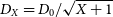 $D_X= D_0/\sqrt{X+1}$
(Lewin et al. Reference Lewin, van Paradijs and Taam1993). As the fractional uncertainty of a nominal PRE distance measurement is independent of X,
$D_X= D_0/\sqrt{X+1}$
(Lewin et al. Reference Lewin, van Paradijs and Taam1993). As the fractional uncertainty of a nominal PRE distance measurement is independent of X,
 $\sigma_X=\sigma_0/\sqrt{1+X}$
, where
$\sigma_X=\sigma_0/\sqrt{1+X}$
, where
 $\sigma_0$
and
$\sigma_0$
and
 $\sigma_X$
represent the uncertainty of the nominal PRE distance at
$\sigma_X$
represent the uncertainty of the nominal PRE distance at
 $X=0$
and at a given X, respectively.
$X=0$
and at a given X, respectively.
Bayes factor
 $K=K^{X=0.7}_{X=0}=P(\pi_1-\pi_0|X=0.7)/P(\pi_1-\pi_0|X=0)$
(ratio of two conditional probabilities), where X refers to the mass fraction of hydrogen of the nuclear fuel
$K=K^{X=0.7}_{X=0}=P(\pi_1-\pi_0|X=0.7)/P(\pi_1-\pi_0|X=0)$
(ratio of two conditional probabilities), where X refers to the mass fraction of hydrogen of the nuclear fuel
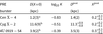
 $^\mathrm{a}$
Chevalier et al. (Reference Chevalier, Ilovaisky, Van Paradijs, Pedersen and Van der Klis1989);
$^\mathrm{a}$
Chevalier et al. (Reference Chevalier, Ilovaisky, Van Paradijs, Pedersen and Van der Klis1989);
 $^\mathrm{b}$
Galloway et al. (Reference Galloway2020).
$^\mathrm{b}$
Galloway et al. (Reference Galloway2020).
As our first attempt to constrain X, we used the calibrated Gaia parallax of each PRE burster to determine which value of X is more likely for the burster –0.73 or 0. We calculated the Bayes factor
 $K=K^{X=0.7}_{X=0}$
using
$K=K^{X=0.7}_{X=0}$
using
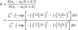 \begin{equation}\begin{split}K &= \frac{\textrm{P}(\pi_1-\pi_0|X=0.7)}{\textrm{P}(\pi_1-\pi_0|X=0)}\\[3pt] &= \frac{\int^{\infty}_{0} \frac{1}{\sigma_{0.7}}\exp\left[-\frac{1}{2}\left(\frac{1/D-\mu_{\pi}}{\sigma_{\pi}}\right)^2-\frac{1}{2}\left(\frac{D-D_{0.7}}{\sigma_{0.7}}\right)^2\right]\textrm{d}D}{\int^{\infty}_{0} \frac{1}{\sigma_{0}}\exp\left[-\frac{1}{2}\left(\frac{1/D-\mu_{\pi}}{\sigma_{\pi}}\right)^2-\frac{1}{2}\left(\frac{D-D_{0}}{\sigma_{0}}\right)^2\right] \textrm{d}D},\end{split}\end{equation}
where
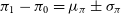 $\pi_1-\pi_0=\mu_{\pi}\pm\sigma_{\pi}$
,
$\pi_1-\pi_0=\mu_{\pi}\pm\sigma_{\pi}$
,
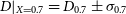 $D|_{X=0.7}=D_{0.7} \pm \sigma_{0.7}$
and
$D|_{X=0.7}=D_{0.7} \pm \sigma_{0.7}$
and
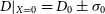 $D|_{X=0}=D_{0} \pm \sigma_{0}$
. For the calculation of
$D|_{X=0}=D_{0} \pm \sigma_{0}$
. For the calculation of
 $K^{X=0.7}_{X=0}$
, we did not use any Galactic prior (see Equation (4) for explanation), as the extra constraint given by a Galactic prior is negligible when X is fixed. The results of
$K^{X=0.7}_{X=0}$
, we did not use any Galactic prior (see Equation (4) for explanation), as the extra constraint given by a Galactic prior is negligible when X is fixed. The results of
 $K^{X=0.7}_{X=0}$
are presented in Table 4.
$K^{X=0.7}_{X=0}$
are presented in Table 4.
Among the three
 $\log_{10} K^{X=0.7}_{X=0}$
values, the one for Cen
$\log_{10} K^{X=0.7}_{X=0}$
values, the one for Cen
 $\textrm{X}-4$
is the most offset from 0, which suggests the calibrated parallax of Cen
$\textrm{X}-4$
is the most offset from 0, which suggests the calibrated parallax of Cen
 $\textrm{X}-4$
substantially (when
$\textrm{X}-4$
substantially (when
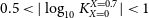 $0.5<|\log_{10}K^{X=0.7}_{X=0}|<1$
, Kass & Raftery Reference Kass and Raftery1995) favours
$0.5<|\log_{10}K^{X=0.7}_{X=0}|<1$
, Kass & Raftery Reference Kass and Raftery1995) favours
 $X=0$
over
$X=0$
over
 $X=0.7$
. Merely 2 PRE bursts have ever been observed from Cen
$X=0.7$
. Merely 2 PRE bursts have ever been observed from Cen
 $\textrm{X}-4$
in 1969 (Belian et al. Reference Belian, Conner and Evans1972) and 1979 (Matsuoka et al. Reference Matsuoka1980). The long intervals between PRE bursts of Cen
$\textrm{X}-4$
in 1969 (Belian et al. Reference Belian, Conner and Evans1972) and 1979 (Matsuoka et al. Reference Matsuoka1980). The long intervals between PRE bursts of Cen
 $\textrm{X}-4$
imply small accretion rates and low X at the time of PRE bursts, despite hydrogen signatures observed from its donor star (e.g. Shahbaz, Watson, & Dhillon, Reference Shahbaz, Watson and Dhillon2014). This expectation is confirmed by the
$\textrm{X}-4$
imply small accretion rates and low X at the time of PRE bursts, despite hydrogen signatures observed from its donor star (e.g. Shahbaz, Watson, & Dhillon, Reference Shahbaz, Watson and Dhillon2014). This expectation is confirmed by the
 $\log_{10} K^{X=0.7}_{X=0}$
of Cen
$\log_{10} K^{X=0.7}_{X=0}$
of Cen
 $\textrm{X}-4$
.
$\textrm{X}-4$
.
It is noteworthy that hydrogen-poor nuclear fuel at the time of PRE bursts is also favoured for Cyg
 $\textrm{X}-2$
and
$\textrm{X}-2$
and
 $4\textrm{U}\,0919-54$
. In fact, the previous independent test of the simplistic PRE model using GC PRE bursters also suggests hydrogen-poor nuclear fuel at the time of PRE bursts for the majority of the 12 GC PRE bursters (Kuulkers et al. Reference Kuulkers, den Hartog, in’t Zand, Verbunt, Harris and Cocchi2003). The statistical inclination towards low X, if confirmed with a larger sample of PRE bursters, might be partly attributed to a selection effect explained as follows.
$4\textrm{U}\,0919-54$
. In fact, the previous independent test of the simplistic PRE model using GC PRE bursters also suggests hydrogen-poor nuclear fuel at the time of PRE bursts for the majority of the 12 GC PRE bursters (Kuulkers et al. Reference Kuulkers, den Hartog, in’t Zand, Verbunt, Harris and Cocchi2003). The statistical inclination towards low X, if confirmed with a larger sample of PRE bursters, might be partly attributed to a selection effect explained as follows.
For each PRE burster, only the brightest PRE bursts are selected to calculate its nominal PRE distance (Galloway et al. Reference Galloway, Muno, Hartman, Psaltis and Chakrabarty2008; Reference Galloway2020; Chevalier et al. Reference Chevalier, Ilovaisky, Van Paradijs, Pedersen and Van der Klis1989). This selection criterion results in a nominal PRE distance that tends to decrease with time as brighter bursts are discovered. This tendency is clearly shown by the fact that almost all the nominal PRE distances registered in Table 9 of Galloway et al. (Reference Galloway, Muno, Hartman, Psaltis and Chakrabarty2008) are larger than their counterparts in Table 8 of Galloway et al. (Reference Galloway2020). If we assume the variability of observed fluxes of PRE bursts is mainly caused by the fluctuation of X (at the time of different PRE bursts), the selection criterion of PRE bursters would lead to an increasingly biased PRE-burst sample that is more likely low-X. This selection effect would have a big impact on the X of the frequent PRE burster Cyg
 $\textrm{X}-2$
(see
$\textrm{X}-2$
(see
 $n_{\textrm{burst}}$
in Table 1 of Galloway et al. Reference Galloway2020), but less so for
$n_{\textrm{burst}}$
in Table 1 of Galloway et al. Reference Galloway2020), but less so for
 $4\textrm{U}\,0919-54$
and Cen
$4\textrm{U}\,0919-54$
and Cen
 $\textrm{X}-4$
. A low X of
$\textrm{X}-4$
. A low X of
 $4\textrm{U}\,0919-54$
(if confirmed in the future) can be explained by the suggestion that the donor star of
$4\textrm{U}\,0919-54$
(if confirmed in the future) can be explained by the suggestion that the donor star of
 $4\textrm{U}\,0919-54$
is likely a helium white dwarf (in’t Zand et al. Reference in’t Zand, Cumming, van der Sluys, Verbunt and Pols2005). On the other hand, the revised nominal PRE distances of PRE bursters (Galloway et al. Reference Galloway2020) relieve the tension between the pre-2008 nominal PRE distances (see the references in Table 1 of A21) and the Gaia DR2 distances (A21), as mentioned in Section 1.
$4\textrm{U}\,0919-54$
is likely a helium white dwarf (in’t Zand et al. Reference in’t Zand, Cumming, van der Sluys, Verbunt and Pols2005). On the other hand, the revised nominal PRE distances of PRE bursters (Galloway et al. Reference Galloway2020) relieve the tension between the pre-2008 nominal PRE distances (see the references in Table 1 of A21) and the Gaia DR2 distances (A21), as mentioned in Section 1.
4.2.2. Refining nominal PRE distances and compositions of nuclear fuel
To better understand the statistical properties of X (and to refine the PRE distance), we subsequently constrained both X and the nominal PRE distance D of each PRE burster with its calibrated parallax in a Bayesian way. The 2-D joint probability distribution (JPD) we applied is
 \begin{equation}\begin{split} \phi &= \phi(D,X\ |\ \pi_1-\pi_0,D_0) \\[3pt] &\propto \phi(\pi_1-\pi_0,D_0\ |\ D,X) \\[3pt] &\propto \rho(D) \exp\left[{-\frac{1}{2}\left( \frac{\frac{1}{D}-\mu_{\pi}}{\sigma_{\pi}}\right)^2-\frac{1}{2}\left( \frac{D-\frac{D_0}{\sqrt{X+1}}}{\frac{\sigma_0}{\sqrt{X+1}}}\right)^2}\right], \\[3pt] & (D>0\ \text{and}\ X \in [0,0.73]),\end{split}\end{equation}
where
 $\rho(D)$
represents the Galactic prior term, i.e., the prior probability of finding a PRE burster at a distance D along a given line of sight. We approached
$\rho(D)$
represents the Galactic prior term, i.e., the prior probability of finding a PRE burster at a distance D along a given line of sight. We approached
 $\rho$
by the Galactic mass distribution of LMXBs, which can be calculated with Equation (5) of Atri et al. (Reference Atri2019) using parameters provided by Grimm et al. (Reference Grimm, Gilfanov and Sunyaev2002); Atri et al. (Reference Atri2019). Among the three components of the Galactic mass density (i.e.
$\rho$
by the Galactic mass distribution of LMXBs, which can be calculated with Equation (5) of Atri et al. (Reference Atri2019) using parameters provided by Grimm et al. (Reference Grimm, Gilfanov and Sunyaev2002); Atri et al. (Reference Atri2019). Among the three components of the Galactic mass density (i.e.
 $\rho_{\textrm{bulge}}$
,
$\rho_{\textrm{bulge}}$
,
 $\rho_{\textrm{disk}}$
, and
$\rho_{\textrm{disk}}$
, and
 $\rho_{\textrm{sphere}}$
, see Grimm et al. Reference Grimm, Gilfanov and Sunyaev2002 for explanations), the Galactic-disk component
$\rho_{\textrm{sphere}}$
, see Grimm et al. Reference Grimm, Gilfanov and Sunyaev2002 for explanations), the Galactic-disk component
 $\rho_{\textrm{disk}}$
dominates the Galactic mass density budget for LMXBs at the light of sight to any of the three PRE bursters. Therefore, for this work alone, we adopted
$\rho_{\textrm{disk}}$
dominates the Galactic mass density budget for LMXBs at the light of sight to any of the three PRE bursters. Therefore, for this work alone, we adopted
 $\rho_{\textrm{disk}}$
(see Equation (5) of Grimm et al. Reference Grimm, Gilfanov and Sunyaev2002) as the Galactic prior term
$\rho_{\textrm{disk}}$
(see Equation (5) of Grimm et al. Reference Grimm, Gilfanov and Sunyaev2002) as the Galactic prior term
 $\rho$
.
$\rho$
.
2-D histograms and marginalised 1-D histograms of posterior distance
 $D^{\textrm{post}}$
and
$D^{\textrm{post}}$
and
 $X'^{\textrm{post}}$
(defined in Section 4.3) simulated with bilby (Ashton et al. Reference Ashton2019) and plotted with corner.py (Foreman-Mackey Reference Foreman-Mackey2016). The n-th contour in each 2-D histogram contains
$X'^{\textrm{post}}$
(defined in Section 4.3) simulated with bilby (Ashton et al. Reference Ashton2019) and plotted with corner.py (Foreman-Mackey Reference Foreman-Mackey2016). The n-th contour in each 2-D histogram contains
 $1-\exp\left(-n^2/2\right)$
of the simulated sample (Foreman-Mackey Reference Foreman-Mackey2016). The vertical lines in the middle and two sides mark the median and central 68% of the sample, respectively.
$1-\exp\left(-n^2/2\right)$
of the simulated sample (Foreman-Mackey Reference Foreman-Mackey2016). The vertical lines in the middle and two sides mark the median and central 68% of the sample, respectively.
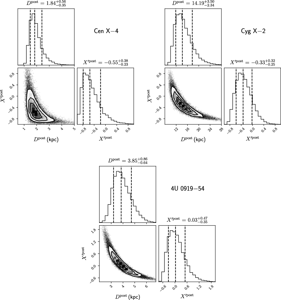
Following the JPD, we simulated posterior {D, X} pairs (hereafter referred to as
 $D^\textrm{post}$
and
$D^\textrm{post}$
and
 $X^\textrm{post}$
), using bilby
Footnote c (Ashton et al. Reference Ashton2019). For this simulation, we adopted a uniform distribution between 0 and 0.73 for X and a uniform distribution between 0 and 50 kpc for D (where using a larger upper limit of D does not change the result). Based on the marginalised probability density functions (PDFs) of the simulated {
$X^\textrm{post}$
), using bilby
Footnote c (Ashton et al. Reference Ashton2019). For this simulation, we adopted a uniform distribution between 0 and 0.73 for X and a uniform distribution between 0 and 50 kpc for D (where using a larger upper limit of D does not change the result). Based on the marginalised probability density functions (PDFs) of the simulated {
 $D^\textrm{post}$
,
$D^\textrm{post}$
,
 $X^\textrm{post}$
} chain, we estimated
$X^\textrm{post}$
} chain, we estimated
 $D^\textrm{post}$
and
$D^\textrm{post}$
and
 $X^\textrm{post}$
, which are presented in Figure 2 and Table 4.
$X^\textrm{post}$
, which are presented in Figure 2 and Table 4.
In general, the conversion of parallax to distance depends on the adopted Galactic prior (Bailer-Jones Reference Bailer-Jones2015). As an example, A21 found that the application of different Galactic priors (e.g. Bailer-Jones et al. Reference Bailer-Jones, Rybizki, Fouesneau, Demleitner and Andrae2021; Atri et al. Reference Atri2019) results in inconsistent distances (see Figure 3 of A21). Unlike A21, we applied an extra constraint on D provided by the PRE distance (see Equation (4)), which gives a handle on X and improves the constraint on D. With this extra constraint, the dependence on the Galactic prior becomes negligible for all of the three PRE bursters: their
 $D^\textrm{post}$
and
$D^\textrm{post}$
and
 $X^\textrm{post}$
stay almost the same without the
$X^\textrm{post}$
stay almost the same without the
 $\rho(D)$
term.
$\rho(D)$
term.
The PDFs of X provide richer information on X than
 $K^{X=0.7}_{X=0}$
. As expected from
$K^{X=0.7}_{X=0}$
. As expected from
 $K^{X=0.7}_{X=0}$
, the PDF of X for Cen
$K^{X=0.7}_{X=0}$
, the PDF of X for Cen
 $\textrm{X}-4$
favours a hydrogen-poor nature of nuclear fuel. In addition to the new constraint we put on X, the nominal PRE distance of each PRE burster incorporating the parallax information is supposed to be more reliable (though not necessarily more precise). We note that the refined nominal PRE distances are still model dependent; their accuracies are subject to the validity of the simplistic PRE model.
$\textrm{X}-4$
favours a hydrogen-poor nature of nuclear fuel. In addition to the new constraint we put on X, the nominal PRE distance of each PRE burster incorporating the parallax information is supposed to be more reliable (though not necessarily more precise). We note that the refined nominal PRE distances are still model dependent; their accuracies are subject to the validity of the simplistic PRE model.
4.3. A roadmap for testing the simplistic PRE model with parallax measurements
The discussion in Section 4.2 is based on the correctness of the simplistic PRE model. Now we discuss the potential feasibility of using parallaxes (of PRE bursters) to test the simplistic PRE model. We first define the PRE distance correction factor
 $\eta$
(
$\eta$
(
 $\eta>0$
) using the relation
$\eta>0$
) using the relation
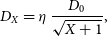 \begin{equation}D_X = \eta\ \frac{D_0}{\sqrt{X+1}},\end{equation}
where
 $D_0$
stands for the nominal PRE distance at
$D_0$
stands for the nominal PRE distance at
 $X=0$
(derived from the simplistic PRE model), and
$X=0$
(derived from the simplistic PRE model), and
 $D_X$
refers to the ‘true’ distance. If the simplistic PRE model is correct, then
$D_X$
refers to the ‘true’ distance. If the simplistic PRE model is correct, then
 $\eta=1$
. However,
$\eta=1$
. However,
 $\eta\ \neq\ 1$
is possible due to various causes including the stochasticity of PRE burst luminosity and anisotropy of PRE burst emission (e.g. Sztajno et al. Reference Sztajno, Fujimoto, van Paradijs, Vacca, Lewin, Penninx and Trumper1987). The latter cause implies
$\eta\ \neq\ 1$
is possible due to various causes including the stochasticity of PRE burst luminosity and anisotropy of PRE burst emission (e.g. Sztajno et al. Reference Sztajno, Fujimoto, van Paradijs, Vacca, Lewin, Penninx and Trumper1987). The latter cause implies
 $\eta$
to be geometry dependent (e.g. viewing-angle-related); if all PRE bursters have different geometry-dependent
$\eta$
to be geometry dependent (e.g. viewing-angle-related); if all PRE bursters have different geometry-dependent
 $\eta$
, a search for a global deviation of
$\eta$
, a search for a global deviation of
 $\eta$
from unity with a sample of PRE bursters would be less practical. Nevertheless, it remains practical to constrain
$\eta$
from unity with a sample of PRE bursters would be less practical. Nevertheless, it remains practical to constrain
 $\eta$
on an individual basis. One way to make this constraint is using the generalised X, defined as
$\eta$
on an individual basis. One way to make this constraint is using the generalised X, defined as
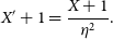 \begin{equation}X'+1=\frac{X+1}{\eta^2}.\end{equation}
Accordingly,
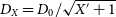 $D_X=D_0/\sqrt{X'+1}$
. Thanks to the same mathematical formalism, we can re-use Equation (4) as the JPD for statistical analysis, except that the domain of
$D_X=D_0/\sqrt{X'+1}$
. Thanks to the same mathematical formalism, we can re-use Equation (4) as the JPD for statistical analysis, except that the domain of
 $X^{\prime}$
is widened to
$X^{\prime}$
is widened to
 $X'>-1$
.
$X'>-1$
.
The simulated {
 $D^{\textrm{post}}$
,
$D^{\textrm{post}}$
,
 $X'^{\textrm{post}}$
} chain (posterior D and
$X'^{\textrm{post}}$
} chain (posterior D and
 $X^{\prime}$
) is depicted in Figure 3. If the simplistic PRE model is correct, then
$X^{\prime}$
) is depicted in Figure 3. If the simplistic PRE model is correct, then
 $\eta=1$
; as a result,
$\eta=1$
; as a result,
 $X^{\prime}$
is supposed to fall into the ‘standard’ domain of [0, 0.73]. None of the three PDFs of
$X^{\prime}$
is supposed to fall into the ‘standard’ domain of [0, 0.73]. None of the three PDFs of
 $X^{\prime}$
decisively rules out
$X^{\prime}$
decisively rules out
 $X^{\prime}$
from this standard domain. However, we notice
$X^{\prime}$
from this standard domain. However, we notice
 $X'<0$
at 90% confidence for Cen
$X'<0$
at 90% confidence for Cen
 $\textrm{X}-4$
, which moderately disfavours the simplistic PRE model.
$\textrm{X}-4$
, which moderately disfavours the simplistic PRE model.
As the domain of
 $X^{\prime}$
is broadened from that of X, the fractional precision of
$X^{\prime}$
is broadened from that of X, the fractional precision of
 $D^{\textrm{post}}$
becomes predominantly reliant on that of the parallax. In this regime,
$D^{\textrm{post}}$
becomes predominantly reliant on that of the parallax. In this regime,
 $D^{\textrm{post}}$
and
$D^{\textrm{post}}$
and
 $X'^{\textrm{post}}$
become more dependent on the adopted Galactic prior. To understand the degree of this dependence, we re-estimated
$X'^{\textrm{post}}$
become more dependent on the adopted Galactic prior. To understand the degree of this dependence, we re-estimated
 $D^{\textrm{post}}$
and
$D^{\textrm{post}}$
and
 $X'^{\textrm{post}}$
after resetting the Galactic prior to
$X'^{\textrm{post}}$
after resetting the Galactic prior to
 $\rho(D)=1$
, which are summarised in Table 5. For Cyg
$\rho(D)=1$
, which are summarised in Table 5. For Cyg
 $\textrm{X}-2$
with insignificant
$\textrm{X}-2$
with insignificant
 $\pi_1-\pi_0$
, the dependence on the Galactic prior is evident, despite the consistency between the two sets of
$\pi_1-\pi_0$
, the dependence on the Galactic prior is evident, despite the consistency between the two sets of
 $D^{\textrm{post}}$
and
$D^{\textrm{post}}$
and
 $X'^{\textrm{post}}$
. For Cen
$X'^{\textrm{post}}$
. For Cen
 $\textrm{X}-4$
and
$\textrm{X}-4$
and
 $4\textrm{U}\,0919-54$
both having relatively significant
$4\textrm{U}\,0919-54$
both having relatively significant
 $\pi_1-\pi_0$
, the degree of the dependence varies with the Galactic coordinates of the targets. In particular, we found the
$\pi_1-\pi_0$
, the degree of the dependence varies with the Galactic coordinates of the targets. In particular, we found the
 $D^{\textrm{post}}$
and
$D^{\textrm{post}}$
and
 $X'^{\textrm{post}}$
of Cen
$X'^{\textrm{post}}$
of Cen
 $\textrm{X}-4$
are robust against the selection of Galactic priors in Equation (4).
$\textrm{X}-4$
are robust against the selection of Galactic priors in Equation (4).
 $D^{\textrm{post}}$
and
$D^{\textrm{post}}$
and
 $X'^{\textrm{post}}$
(see Section 4.3) inferred from the Galactic prior
$X'^{\textrm{post}}$
(see Section 4.3) inferred from the Galactic prior
 $\rho(D)$
of Equation (4), in comparison to the counterparts (noted as
$\rho(D)$
of Equation (4), in comparison to the counterparts (noted as
 $\tilde{D}^{\textrm{post}}$
and
$\tilde{D}^{\textrm{post}}$
and
 $\tilde{X'}^{\textrm{post}}$
) given
$\tilde{X'}^{\textrm{post}}$
) given
 $\rho(D)=1$
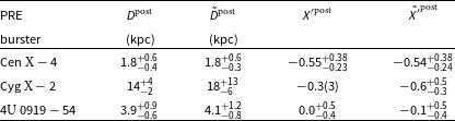
Using
 $X^{\prime}$
as a probe of the simplistic PRE model has the advantage of being independent of the PDF for X, which is usually not available. Future
$X^{\prime}$
as a probe of the simplistic PRE model has the advantage of being independent of the PDF for X, which is usually not available. Future
 $D_0$
and
$D_0$
and
 $\pi_1-\pi_0$
measurements with higher precision will sharpen the above test of the simplistic PRE model. Lower fractional uncertainty of
$\pi_1-\pi_0$
measurements with higher precision will sharpen the above test of the simplistic PRE model. Lower fractional uncertainty of
 $\pi_1-\pi_0$
will not only reduce the strong correlation between
$\pi_1-\pi_0$
will not only reduce the strong correlation between
 $D^{\textrm{post}}$
and
$D^{\textrm{post}}$
and
 $X'^{\textrm{post}}$
for Cyg
$X'^{\textrm{post}}$
for Cyg
 $\textrm{X}-2$
and
$\textrm{X}-2$
and
 $4\textrm{U}\,0919-54$
(shown in Figure 3) but also lessen the dependence of inferred
$4\textrm{U}\,0919-54$
(shown in Figure 3) but also lessen the dependence of inferred
 $D^{\textrm{post}}$
and
$D^{\textrm{post}}$
and
 $X'^{\textrm{post}}$
on the adopted Galactic prior. On the other hand, constraining X at PRE bursts independently (with, for example, ignition models of X-ray bursts) is the key to singling out
$X'^{\textrm{post}}$
on the adopted Galactic prior. On the other hand, constraining X at PRE bursts independently (with, for example, ignition models of X-ray bursts) is the key to singling out
 $\eta$
. Given that the simplistic PRE model is not significantly disfavoured by any of the 3 PRE bursters, the refined distances in Table 4 (based on the correctness of the simplistic PRE model) are still valid.
$\eta$
. Given that the simplistic PRE model is not significantly disfavoured by any of the 3 PRE bursters, the refined distances in Table 4 (based on the correctness of the simplistic PRE model) are still valid.
4.4. Future prospects
The potential of constraining X and testing the simplistic PRE model using Gaia parallaxes of PRE bursters hinges on the achievable parallax uncertainties. Future Gaia data releases include Gaia Data Release 4 (DR4) (for the 5-yr data collection) and the data release after extended observations of up to 5.4 yr (https://www.cosmos.esa.int/web/gaia/release). We predict the achievable parallax (
 $\pi_1$
) and proper motion uncertainties of Cen
$\pi_1$
) and proper motion uncertainties of Cen
 $\textrm{X}-4$
for future Gaia data releases using the simulation method detailed in Appendix A. In the same way, we estimated the predicted
$\textrm{X}-4$
for future Gaia data releases using the simulation method detailed in Appendix A. In the same way, we estimated the predicted
 $\pi_1$
uncertainty
$\pi_1$
uncertainty
 $\hat{\sigma}_{\pi_1}$
of Cyg
$\hat{\sigma}_{\pi_1}$
of Cyg
 $\textrm{X}-2$
,
$\textrm{X}-2$
,
 $4\textrm{U}\,0919-54$
, and XB 2129+47 for future data releases and DR2, which are listed in Table 6. The predicted
$4\textrm{U}\,0919-54$
, and XB 2129+47 for future data releases and DR2, which are listed in Table 6. The predicted
 $\pi_1$
uncertainties for DR2, denoted as
$\pi_1$
uncertainties for DR2, denoted as
 $\hat{\sigma}^\textrm{DR2}_{\pi_1}$
, generally agree with the real values
$\hat{\sigma}^\textrm{DR2}_{\pi_1}$
, generally agree with the real values
 $\sigma^\textrm{DR2}_{\pi_1}$
(see Table 6). In general, our simulation shows Gaia parallax and proper motion precision improves with observation time t at roughly
$\sigma^\textrm{DR2}_{\pi_1}$
(see Table 6). In general, our simulation shows Gaia parallax and proper motion precision improves with observation time t at roughly
 $t^{-1/2}$
and
$t^{-1/2}$
and
 $t^{-3/2}$
, respectively.
$t^{-3/2}$
, respectively.
Predicted parallax (
 $\pi_1$
) uncertainties
$\pi_1$
) uncertainties
 $\hat{\sigma}_{\pi_1}$
for Cen
$\hat{\sigma}_{\pi_1}$
for Cen
 $\textrm{X}-4$
, Cyg
$\textrm{X}-4$
, Cyg
 $\textrm{X}-2$
, and
$\textrm{X}-2$
, and
 $4\textrm{U}\,0919-54$
obtained with simulations (see Appendix A for details). For comparison, real values of
$4\textrm{U}\,0919-54$
obtained with simulations (see Appendix A for details). For comparison, real values of
 $\sigma^\textrm{DR2}_{\pi_1}$
are provided as
$\sigma^\textrm{DR2}_{\pi_1}$
are provided as
 $\sigma^\textrm{DR2}_{\pi_1}$
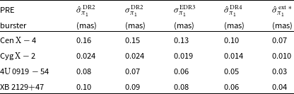
 $^*$
we adopt an indicative 5-yr extension on top of the Gaia 5-yr mission.
$^*$
we adopt an indicative 5-yr extension on top of the Gaia 5-yr mission.
According to Table 3, the future parallax uncertainty of Cyg
 $\textrm{X}-2$
will be predominantly limited by the uncertainty of
$\textrm{X}-2$
will be predominantly limited by the uncertainty of
 $\pi_0$
, or
$\pi_0$
, or
 $\sigma_{\pi_0}$
. For this target, improvement in the estimation of the zero-point parallax correction and its uncertainty – which is challenging due to the relative brightness of the source – is essential. In comparison, the
$\sigma_{\pi_0}$
. For this target, improvement in the estimation of the zero-point parallax correction and its uncertainty – which is challenging due to the relative brightness of the source – is essential. In comparison, the
 $\sigma_{\pi_1}$
of Cen
$\sigma_{\pi_1}$
of Cen
 $\textrm{X}-4$
,
$\textrm{X}-4$
,
 $4\textrm{U}\,0919-54$
, and XB 2129+47 dominates the respective error budget of the calibrated parallax
$4\textrm{U}\,0919-54$
, and XB 2129+47 dominates the respective error budget of the calibrated parallax
 $\pi_1-\pi_0$
. Therefore, one can expect
$\pi_1-\pi_0$
. Therefore, one can expect
 $\pi_1-\pi_0$
of Cen
$\pi_1-\pi_0$
of Cen
 $\textrm{X}-4$
,
$\textrm{X}-4$
,
 $4\textrm{U}\,0919-54$
, and XB 2129+47 to be potentially 1.9 times more precise (than EDR3) at the end of the extended Gaia mission (with 10-yr data), which would promise better constraints on X and
$4\textrm{U}\,0919-54$
, and XB 2129+47 to be potentially 1.9 times more precise (than EDR3) at the end of the extended Gaia mission (with 10-yr data), which would promise better constraints on X and
 $X^{\prime}$
for Cen
$X^{\prime}$
for Cen
 $\textrm{X}-4$
and
$\textrm{X}-4$
and
 $4\textrm{U}\,0919-54$
. On the other hand, to constrain X and
$4\textrm{U}\,0919-54$
. On the other hand, to constrain X and
 $X^{\prime}$
for XB 2129+47 with its already relatively precise Gaia parallax will require more PRE bursts to be detected from XB 2129+47. Apart from Gaia astrometry, radio observations of PRE bursters during their outbursts using very long baseline interferometry technique can also potentially measure geometric parallaxes of PRE bursters, hence serving the same scientific goals outlined in this paper.
$X^{\prime}$
for XB 2129+47 with its already relatively precise Gaia parallax will require more PRE bursts to be detected from XB 2129+47. Apart from Gaia astrometry, radio observations of PRE bursters during their outbursts using very long baseline interferometry technique can also potentially measure geometric parallaxes of PRE bursters, hence serving the same scientific goals outlined in this paper.
This work only deals with the simplistic PRE model, the hitherto most impactful PRE model. As is mentioned in Section 1, PRE models are not the only pathway to the distances of type I X-ray bursters. Bayesian inference based on a burst ignition model (Cumming & Bildsten Reference Cumming and Bildsten2000) was recently realised to estimate parameters including X and D (Goodwin et al. Reference Goodwin, Galloway, Heger, Cumming and Johnston2019). We believe such inferences will be made for more type I X-ray bursters in the near future. In Bayesian analysis based on burst ignition models (e.g. Cumming & Bildsten Reference Cumming and Bildsten2000; Woosley et al. Reference Woosley2004), model-independent geometric parallaxes will serve as prior knowledge and help refine the inferred parameters including D and X; the parallaxes can also judge which burst ignition model is more likely correct with a Bayes factor analysis.
Finally, we reiterate that we have assumed
 $M_{\textrm{NS}}=1.4\,\textrm{M}_{\odot}$
and
$M_{\textrm{NS}}=1.4\,\textrm{M}_{\odot}$
and
 $R_{\textrm{NS}}=11.2$
km for all PRE bursters. Therefore, strictly speaking,
$R_{\textrm{NS}}=11.2$
km for all PRE bursters. Therefore, strictly speaking,
 $\eta$
should also reflect the deviation of
$\eta$
should also reflect the deviation of
 $M_{\textrm{NS}}$
and
$M_{\textrm{NS}}$
and
 $R_{\textrm{NS}}$
from their respective assumed values. Though a large deviation of
$R_{\textrm{NS}}$
from their respective assumed values. Though a large deviation of
 $M_{\textrm{NS}}$
from 1.4
$M_{\textrm{NS}}$
from 1.4
 $\textrm{M}_{\odot}$
is rare, it is not impossible (Shao et al. Reference Shao, Tang, Jiang and Fan2020). In general,
$\textrm{M}_{\odot}$
is rare, it is not impossible (Shao et al. Reference Shao, Tang, Jiang and Fan2020). In general,
 $L_{\textrm{Edd},\infty}$
would increase with larger
$L_{\textrm{Edd},\infty}$
would increase with larger
 $M_{\textrm{NS}}$
and
$M_{\textrm{NS}}$
and
 $R_{\textrm{NS}}$
(see Equation (1)). For example,
$R_{\textrm{NS}}$
(see Equation (1)). For example,
 $L_{\textrm{Edd},\infty}(M_{\textrm{NS}}=2, R_{\textrm{NS}}=15)$
is 40% greater than
$L_{\textrm{Edd},\infty}(M_{\textrm{NS}}=2, R_{\textrm{NS}}=15)$
is 40% greater than
 $L_{\textrm{Edd},\infty}(M_{\textrm{NS}}=1.4, R_{\textrm{NS}}=11.2)$
. Such a
$L_{\textrm{Edd},\infty}(M_{\textrm{NS}}=1.4, R_{\textrm{NS}}=11.2)$
. Such a
 $L_{\textrm{Edd},\infty}$
would correspond to
$L_{\textrm{Edd},\infty}$
would correspond to
 $X'=-0.29$
assuming
$X'=-0.29$
assuming
 $X=0$
and the simplistic PRE model is correct. This value is consistent with
$X=0$
and the simplistic PRE model is correct. This value is consistent with
 $X'=-0.55^{+0.38}_{-0.23}$
for Cen
$X'=-0.55^{+0.38}_{-0.23}$
for Cen
 $\textrm{X}-4$
. Given that the NS mass distribution is relatively well constrained compared to the NS radius distribution, it is possible to constrain the NS radius of a PRE burster in a Bayesian framework (slightly different from this work) provided prior knowledge of X, D, and
$\textrm{X}-4$
. Given that the NS mass distribution is relatively well constrained compared to the NS radius distribution, it is possible to constrain the NS radius of a PRE burster in a Bayesian framework (slightly different from this work) provided prior knowledge of X, D, and
 $M_{\textrm{NS}}$
, assuming the simplistic PRE model is correct.
$M_{\textrm{NS}}$
, assuming the simplistic PRE model is correct.
5. Conclusion
This work joins the few previous efforts to determine the Gaia parallax zero-point
 $\pi_0$
for a single source using nearby (on the sky) background quasars. We provide a new template for
$\pi_0$
for a single source using nearby (on the sky) background quasars. We provide a new template for
 $\pi_0$
determination (which also includes the
$\pi_0$
determination (which also includes the
 $\pi_0$
uncertainty) approached by the weighted standard deviation of quasar parallaxes with respect to the filter parameters (see Section 3). This work focuses on the small sample of PRE bursters with detected Gaia parallaxes
$\pi_0$
uncertainty) approached by the weighted standard deviation of quasar parallaxes with respect to the filter parameters (see Section 3). This work focuses on the small sample of PRE bursters with detected Gaia parallaxes
 $\pi_1$
. A future work will apply the new template to a larger sample of targets, which can enable a comprehensive comparison with zero-parallax points estimated in other ways.
$\pi_1$
. A future work will apply the new template to a larger sample of targets, which can enable a comprehensive comparison with zero-parallax points estimated in other ways.
We also introduce a Bayesian framework to test the simplistic PRE model with parallaxes of PRE bursters on an individual basis. Though no parallax of the PRE bursters decisively disfavours the simplistic PRE model, the model is disfavoured by the current Cen
 $\textrm{X}-4$
parallax at 90% confidence. At the end of the extended Gaia mission with 10-yr data, we expect the parallax precision to improve by a factor of 1.9, which will sharpen the test of the simplistic PRE model. This test will also considerably benefit from an independent determination of X (hydrogen mass fraction of nuclear fuel), which we highly encourage.
$\textrm{X}-4$
parallax at 90% confidence. At the end of the extended Gaia mission with 10-yr data, we expect the parallax precision to improve by a factor of 1.9, which will sharpen the test of the simplistic PRE model. This test will also considerably benefit from an independent determination of X (hydrogen mass fraction of nuclear fuel), which we highly encourage.
Acknowledgements
The authors thank Ilya Mandel, Chris Flynn, and Adelle Goodwin for useful discussions and are grateful to the anonymous referee for the helpful comments on the manuscript. H.D. is supported by the ACAMAR (Australia-ChinA ConsortiuM for Astrophysical Research) scholarship, which is partly funded by the China Scholarship Council. A.T.D is the recipient of an ARC Future Fellowship (FT150100415). Parts of this research were conducted by the Australian Research Council Centre of Excellence for Gravitational Wave Discovery (OzGrav), through project number CE170100004. This work has made use of data from the European Space Agency (ESA) mission Gaia (https://www.cosmos.esa.int/gaia), processed by the Gaia Data Processing and Analysis Consortium (DPAC, https://www.cosmos.esa.int/web/gaia/dpac/consortium). Data analysis was partly performed on OzSTAR, the Swinburne-based supercomputer.
A. Simulating the parallax precision of Cen
$\textbf{X}-\textbf{4}$
in future Gaia data releases

To simulate the uncalibrated parallax (
 $\pi_1$
) precision of Cen
$\pi_1$
) precision of Cen
 $\textrm{X}-4$
for a future Gaia data release, we made two assumptions: (1) Cen
$\textrm{X}-4$
for a future Gaia data release, we made two assumptions: (1) Cen
 $\textrm{X}-4$
is observed by Gaia at equal intervals; (2)
$\textrm{X}-4$
is observed by Gaia at equal intervals; (2)
 $\sigma^i_k=\sigma^j_k$
, (
$\sigma^i_k=\sigma^j_k$
, (
 $k=\alpha, \delta$
and
$k=\alpha, \delta$
and
 $i \neq j$
), where
$i \neq j$
), where
 $\sigma^i_{\alpha}$
and
$\sigma^i_{\alpha}$
and
 $\sigma^i_{\delta}$
stand for, respectively, the uncertainty of right ascension (RA) and declination at the i-th observation.
$\sigma^i_{\delta}$
stand for, respectively, the uncertainty of right ascension (RA) and declination at the i-th observation.
The observation interval is determined with Table 1 of Gaia Collaboration et al. (2016). At the ecliptic latitude of Cen
 $\textrm{X}-4$
(
$\textrm{X}-4$
(
 $-14^\circ1$
), the number of observations is 63 over 5 yr, corresponding to an interval of 29 d. It appears from Table 2 that, for a specific target,
$-14^\circ1$
), the number of observations is 63 over 5 yr, corresponding to an interval of 29 d. It appears from Table 2 that, for a specific target,
 $\sigma_{\alpha}/\sigma_{\delta} \approx \sigma_{\mu_{\alpha}}/\sigma_{\mu_{\delta}}$
(where
$\sigma_{\alpha}/\sigma_{\delta} \approx \sigma_{\mu_{\alpha}}/\sigma_{\mu_{\delta}}$
(where
 $\sigma_{\mu_{\alpha}}$
and
$\sigma_{\mu_{\alpha}}$
and
 $\sigma_{\mu_{\delta}}$
represent uncertainty of
$\sigma_{\mu_{\delta}}$
represent uncertainty of
 $\mu_{\alpha}$
and
$\mu_{\alpha}$
and
 $\mu_{\delta}$
, respectively), which implies the ratio of spatial resolution between RA and declination deviates slightly from unity and changes with pointing. Hence, we set
$\mu_{\delta}$
, respectively), which implies the ratio of spatial resolution between RA and declination deviates slightly from unity and changes with pointing. Hence, we set
 $\sigma^i_{\alpha} / \sigma^i_{\delta}$
to 1.21, which is the
$\sigma^i_{\alpha} / \sigma^i_{\delta}$
to 1.21, which is the
 $\sigma_{\mu_{\alpha}}/\sigma_{\mu_{\delta}}$
of Cen
$\sigma_{\mu_{\alpha}}/\sigma_{\mu_{\delta}}$
of Cen
 $\textrm{X}-4$
from EDR3.
$\textrm{X}-4$
from EDR3.
Simulated positions of Cen
 $\textrm{X}-4$
were generated with pmpar (available at https://github.com/walterfb/pmpar) using the ‘predictor mode’, based on the astrometric parameters of Cen
$\textrm{X}-4$
were generated with pmpar (available at https://github.com/walterfb/pmpar) using the ‘predictor mode’, based on the astrometric parameters of Cen
 $\textrm{X}\unicode{x002D}4$
in Table 2. We first simulated positions from MJD 56863 to MJD 57901 (the observing period of EDR3). The sole variable
$\textrm{X}\unicode{x002D}4$
in Table 2. We first simulated positions from MJD 56863 to MJD 57901 (the observing period of EDR3). The sole variable
 $\sigma^i_{\alpha}$
(and
$\sigma^i_{\alpha}$
(and
 $\sigma^i_{\delta}$
accordingly) was tuned to make the parallax precision equal to 0.13 mas, the current parallax precision of Cen
$\sigma^i_{\delta}$
accordingly) was tuned to make the parallax precision equal to 0.13 mas, the current parallax precision of Cen
 $\textrm{X}-4$
. Subsequently, we stuck to the position uncertainties while extending the observing period to MJD 58689 (around the end day of the 5-yr period) and MJD 60516 (an indicative day 10 years after the first light of Gaia), which, respectively, yield parallax uncertainties of 0.095 mas and 0.067 mas. Thus, we predict the parallax precision of Cen
$\textrm{X}-4$
. Subsequently, we stuck to the position uncertainties while extending the observing period to MJD 58689 (around the end day of the 5-yr period) and MJD 60516 (an indicative day 10 years after the first light of Gaia), which, respectively, yield parallax uncertainties of 0.095 mas and 0.067 mas. Thus, we predict the parallax precision of Cen
 $\textrm{X}-4$
to improve by a factor of 1.3 and 1.9, respectively, with DR4 and 10-yr data. Besides, we expect the proper motion precision of Cen
$\textrm{X}-4$
to improve by a factor of 1.3 and 1.9, respectively, with DR4 and 10-yr data. Besides, we expect the proper motion precision of Cen
 $\textrm{X}-4$
to be enhanced by 2.7 and 6.7 times, respectively, with DR4 and 10-yr data.
$\textrm{X}-4$
to be enhanced by 2.7 and 6.7 times, respectively, with DR4 and 10-yr data.


