1. Introduction
Clusters of galaxies are formed through often highly energetic merger events and accretion from filaments of the Cosmic Web. Clusters are comprised of constituent galaxies, X-ray emitting plasmas, and
 $\sim\!{\mu G}$
-level magnetic fields (Clarke et al. Reference Clarke, Kronberg and Böhringer2001; Johnston-Hollitt Reference Johnston-Hollitt2003). In a fraction of clusters, large-scale (
$\sim\!{\mu G}$
-level magnetic fields (Clarke et al. Reference Clarke, Kronberg and Böhringer2001; Johnston-Hollitt Reference Johnston-Hollitt2003). In a fraction of clusters, large-scale (
 $\sim\!1$
Mpc) steep-spectrum (
$\sim\!1$
Mpc) steep-spectrum (
 $\alpha \lesssim -1$
Footnote
a
), diffuse radio emission is observed as centrally-located radio halos and peripherally-located radio relics (see van Weeren et al. Reference van Weeren, de Gasperin, Akamatsu, Brüggen, Feretti, Kang, Stroe and Zandanel2019, and references therein). These large-scale synchtrotron-emitting sources are not thought to be presently fuelled by active galactic nuclei (AGN), rather they are assumed to be generated through in situ (re-)acceleration of particles (e.g. Jaffe Reference Jaffe1977; Enßlin et al. Reference Enßlin, Biermann, Klein and Kohle1998). Such sources are observed in predominantly merging, or otherwise morphologically disturbed clusters (e.g. Buote Reference Buote2001; Brunetti et al. Reference Brunetti, Cassano, Dolag and Setti2009; Cassano et al. Reference Cassano, Ettori, Giacintucci, Brunetti, Markevitch, Venturi and Gitti2010; Botteon et al. Reference Botteon2018; Golovich et al. Reference Golovich2019).
$\alpha \lesssim -1$
Footnote
a
), diffuse radio emission is observed as centrally-located radio halos and peripherally-located radio relics (see van Weeren et al. Reference van Weeren, de Gasperin, Akamatsu, Brüggen, Feretti, Kang, Stroe and Zandanel2019, and references therein). These large-scale synchtrotron-emitting sources are not thought to be presently fuelled by active galactic nuclei (AGN), rather they are assumed to be generated through in situ (re-)acceleration of particles (e.g. Jaffe Reference Jaffe1977; Enßlin et al. Reference Enßlin, Biermann, Klein and Kohle1998). Such sources are observed in predominantly merging, or otherwise morphologically disturbed clusters (e.g. Buote Reference Buote2001; Brunetti et al. Reference Brunetti, Cassano, Dolag and Setti2009; Cassano et al. Reference Cassano, Ettori, Giacintucci, Brunetti, Markevitch, Venturi and Gitti2010; Botteon et al. Reference Botteon2018; Golovich et al. Reference Golovich2019).
Radio halos are generally spatially correlated with the thermal, X-ray–emitting core of the cluster and are observed with morhpologies ranging from circular (e.g. Orrú et al. Reference Orrú, Murgia, Feretti, Govoni, Brunetti, Giovannini, Girardi and Setti2007; Murgia et al. Reference Murgia, Govoni, Markevitch, Feretti, Giovannini, Taylor and Carretti2009) to more complex and elongated structures (e.g. van Weeren et al. Reference van Weeren, Röttgering, Intema, Rudnick, Brüggen, Hoeft and Oonk2012). Radio halos are generally observed to have power law spectra, though some halos with significant spectral coverage show steepening beyond GHz frequencies (Thierbach et al. Reference Thierbach, Klein and Wielebinski2003; Xie et al. Reference Xie2020; Rajpurohit et al. Reference Rajpurohit2021c). Merger-driven turbulence in the intra-cluster medium (ICM) may provide a mechanism for in situ (re-)acceleration of seed particles from either the thermal pool of electrons or from a pre-accelerated population of mildly-relativistic ‘fossil’ electrons throughout the cluster volume (e.g. Brunetti et al. Reference Brunetti, Setti, Feretti and Giovannini2001; Buote Reference Buote2001; Brunetti & Jones Reference Brunetti and Jones2014).
Radio relics occur in the low-density cluster outskirts, where strong shocks in the ICM are thought to (re-)accelerate electrons through diffusive-shock acceleration (DSA; e.g. Enßlin et al. Reference Enßlin, Biermann, Klein and Kohle1998, and similar processes; e.g. Kang Reference Kang2015) either originating a ‘fossil’ electron population (e.g. Markevitch et al. Reference Markevitch, Govoni, Brunetti and Jerius2005; Kang & Ryu Reference Kang and Ryu2011; Kang & Ryu Reference Kang and Ryu2016) or accelerated from the thermal pool of electrons in the cluster (e.g. Enßlin et al. Reference Enßlin, Biermann, Klein and Kohle1998; Hoeft & Brüggen Reference Hoeft and Brüggen2007). Unlike radio halos, relics are often observed with highly ordered, linearly polarised emission (e.g. Johnston-Hollitt Reference Johnston-Hollitt2003; van Weeren et al. Reference van Weeren, Röttgering, Brüggen and Hoeft2010; Pearce et al. Reference Pearce2017). The integrated spectra of relics are generally power laws (e.g. Hindson et al. Reference Hindson2014; Loi et al. Reference Loi2017; Rajpurohit et al. Reference Rajpurohit2020; Duchesne et al. Reference Duchesne, Johnston-Hollitt, Bartalucci, Hodgson and Pratt2021a), though few examples exist with curvature beyond GHz frequencies (e.g. Trasatti et al. Reference Trasatti, Akamatsu, Lovisari, Klein, Bonafede, Brüggen, Dallacasa and Clarke2015). In some cases, radio relics have been observed to be located co-spatially with X-ray shocks/surface brightness discontinuities (e.g. Finoguenov et al. Reference Finoguenov, Sarazin, Nakazawa, Wik and Clarke2010; Botteon et al. Reference Botteon, Gastaldello, Brunetti and Dallacasa2016a; Botteon et al. Reference Botteon, Gastaldello, Brunetti and Kale2016b).
Along with the large-scale radio halos and relics, other diffuse, non-thermal sources have been observed in clusters with many observational and physical similarities (see e.g. van Weeren et al. Reference van Weeren, de Gasperin, Akamatsu, Brüggen, Feretti, Kang, Stroe and Zandanel2019, for a review of source types and nomenclature). Radio mini-halos are
 $\lesssim\!500$
kpc synchrotron-emitting regions surrounding AGN in the centres of some cool-core (CC) clusters (see e.g. Bravi et al. Reference Bravi, Gitti and Brunetti2016; Giacintucci et al. Reference Giacintucci, Markevitch, Cassano, Venturi, Clarke, Kale and Cuciti2019). Observationally, they appear as small radio halos with similar spectral and morphological properties but are thought to form via re-acceleration of AGN outflow from small-scale turbulence and sloshing within the cluster core (e.g. Gitti et al. Reference Gitti, Brunetti and Setti2002). Mini-halos are not typically associated with major mergers.
$\lesssim\!500$
kpc synchrotron-emitting regions surrounding AGN in the centres of some cool-core (CC) clusters (see e.g. Bravi et al. Reference Bravi, Gitti and Brunetti2016; Giacintucci et al. Reference Giacintucci, Markevitch, Cassano, Venturi, Clarke, Kale and Cuciti2019). Observationally, they appear as small radio halos with similar spectral and morphological properties but are thought to form via re-acceleration of AGN outflow from small-scale turbulence and sloshing within the cluster core (e.g. Gitti et al. Reference Gitti, Brunetti and Setti2002). Mini-halos are not typically associated with major mergers.
Beyond the cluster core, smaller-scale relic-like sources of various types are also found: radio phoenices or otherwise revived fossil sources have been observed (e.g. Slee et al. Reference Slee, Roy, Murgia, Andernach and Ehle2001; Cohen & Clarke Reference Cohen and Clarke2011; Giacintucci et al. Reference Giacintucci, Markevitch, Johnston-Hollitt, Wik, Wang and Clarke2020; Hodgson et al. Reference Hodgson, Bartalucci, Johnston-Hollitt, McKinley, Vazza and Wittor2021). These sources are typically on the order of a few hundred kpc in size and vary morphologically. They range from ultra-steep spectrum fossil plasmas that have possibly been revived via shock-driven adiabatic compression (e.g. Enßlin & Gopal-Krishna Reference Enßlin and Gopal2001; Enßlin & Brüggen Reference Enßlin and Brüggen2002), radio galaxies with shocks passing through an outer lobe/tail, re-energising the radio plasma (e.g. gentle re-energisation; de Gasperin et al. Reference de Gasperin2017, or less-gentle processes; Bonafede et al. Reference Bonafede, Intema, Brüggen, Girardi, Nonino, Kantharia, van Weeren and Röttgering2014; van Weeren et al. Reference van Weeren2017), to true remnant radio galaxies with no evidence of re-energisation and are simply fading from normal energy losses after their AGN have switched off or have entered a low-power state (e.g. Parma et al. Reference Parma, Murgia, de Ruiter, Fanti, Mack and Govoni2007; Murgia et al. Reference Murgia2011). Distinguishing between what are effectively radio galaxies at various stages through their life-cycle is difficult and in the case of radio phoenices often the hosting cluster does not show evidence of merger-driven shocks. Finally, in rare cases synchrotron-emitting bridges have been observed between cluster pairs (e.g. Govoni et al. Reference Govoni2019; Botteon et al. Reference Botteon2020a), likely formed through turbulence in the inter-cluster region (Brunetti & Vazza Reference Brunetti and Vazza2020).
It is not yet clear whether the seed electrons responsible for radio halos and relics are from the thermal pool or from fossils that have diffused into the surrounding ICM—observations of spectra of such sources are beginning to provide answers (e.g. Rajpurohit et al. Reference Rajpurohit2021c; Rajpurohit et al. Reference Rajpurohit2021b; Rajpurohit et al. Reference Rajpurohit2021a). The current generation of radio interferometers, including the Murchison Widefield Array (MWA; Tingay et al. Reference Tingay2013; Wayth et al. Reference Wayth2018), the Australian Square Kilometre Array Pathfinder (ASKAP; Hotan et al. Reference Hotan2021), the LOw Frequency ARray (LOFAR; van Haarlem et al. Reference van Haarlem2013), and MeerKATFootnote b (Jonas & MeerKAT Team Reference Jonas2016) are beginning to uncover diffuse cluster sources at higher rates (e.g. Wilber et al. Reference Wilber, Johnston-Hollitt, Duchesne, Tasse, Akamatsu, Intema and Hodgson2020; Duchesne et al. Reference Duchesne, Johnston-Hollitt, Zhu, Wayth and Line2020; Di Gennaro et al. Reference Di Gennaro2020; Brüggen et al. Reference Brüggen2021; van Weeren et al. Reference van Weeren2020; Knowles et al. Reference Knowles2021; Duchesne et al. Reference Duchesne, Johnston-Hollitt, Bartalucci, Hodgson and Pratt2021a; Hodgson et al. Reference Hodgson, Bartalucci, Johnston-Hollitt, McKinley, Vazza and Wittor2021; Duchesne et al. Reference Duchesne, Johnston-Hollitt, Offringa, Pratt, Zheng and Dehghan2021b; Duchesne et al. Reference Duchesne, Johnston-Hollitt and Wilber2021c), providing unprecedented insight into cluster diffuse source populations, paving the way for future observations with the Square Kilometre Array (SKA). In this work we detail a targeted campaign to follow-up diffuse radio emission in clusters originally detected in MWA surveys, leveraging the wide bandwidth of the MWA to investigate the low-frequency integrated spectra of these sources.
Throughout this paper, we assume a standard
 $\Lambda$
Cold Dark Matter cosmology with
$\Lambda$
Cold Dark Matter cosmology with
 $H_0 = 70$
km s−1 Mpc−1,
$H_0 = 70$
km s−1 Mpc−1,
 $\Omega_{\rm{M}} = 0.3$
, and
$\Omega_{\rm{M}} = 0.3$
, and
 $\Omega_\Lambda = 1-\Omega_{\rm{M}}$
. Unless otherwise stated, frequency subscripts and superscripts on quantities are in units of MHz.
$\Omega_\Lambda = 1-\Omega_{\rm{M}}$
. Unless otherwise stated, frequency subscripts and superscripts on quantities are in units of MHz.
2. Data & methods
2.1. Cluster sample
(Duchesne et al. Reference Duchesne, Johnston-Hollitt, Offringa, Pratt, Zheng and Dehghan2021b, hereafter D21) report a number of candidate diffuse cluster sources detected in a large, deep
 $45^\circ \times 45^\circ$
MWA image created for foreground modelling of the Epoch of Re-ionisation 0-h field (Offringa et al. Reference Offringa2016). Due to the low resolution of the MWA, many of these sources had an uncertain nature. With the upgrade to the Phase 2 ‘extended’ MWA (Wayth et al. Reference Wayth2018, hereafter MWA-2) and the allure of an increase in resolution by a factor of two, we carried out re-observation of a selection of these sources as part of MWA project G0045 with Director’s Time observations of two additional fields and the addition of overlapping archival observations.
$45^\circ \times 45^\circ$
MWA image created for foreground modelling of the Epoch of Re-ionisation 0-h field (Offringa et al. Reference Offringa2016). Due to the low resolution of the MWA, many of these sources had an uncertain nature. With the upgrade to the Phase 2 ‘extended’ MWA (Wayth et al. Reference Wayth2018, hereafter MWA-2) and the allure of an increase in resolution by a factor of two, we carried out re-observation of a selection of these sources as part of MWA project G0045 with Director’s Time observations of two additional fields and the addition of overlapping archival observations.
At the same time, a candidate list of diffuse cluster sources had been prepared based on visual searches of the GaLactic and Extragalactic MWA (GLEAM) survey (Wayth et al. Reference Wayth2015; Hurley-Walker et al. Reference Hurley-Walker2017). These searches focused on clusters from the Meta-Catalogue of X-ray detected Clusters (MCXC; Piffaretti et al. Reference Piffaretti, Arnaud, Pratt, Pointecouteau and Melin2011), the Abell catalogues (Abell Reference Abell1958; Abell et al. Reference Abell, Corwin and Olowin1989), Planck Sunyaev–Zel’dovich clusters (Planck Collaboration et al. Reference Planck2015; Planck Collaboration et al. Reference Planck2016), and a handful of miscellaneous clusters serendipitously found to host candidate diffuse emission that are nearby other clusters from the aforementioned catalogues. While the full sample is not within the scope of this work (it would be prohibitive to perform targeted follow-up of close to 200 sources), we present here 31 sources across 9 fieldsFootnote
c
. Due to the large field of view of the MWA (
 $\sim\!20$
deg at 216 MHz and
$\sim\!20$
deg at 216 MHz and
 $\sim\!60$
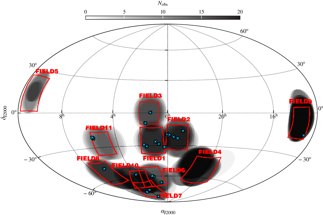
deg at 88 MHz) we planned MWA-2 observations to cover a total 22 clusters (Table 1). While the 200-MHz wideband GLEAM image is usually sufficient to detect and measure flux density of these sources, the lower-frequency bands become prohibitively confused for use here. The fields observed (labelled FIELD1–FIELD11) are shown on Figure 1. FIELD5 and our target source within Abell 1127 were presented in Duchesne et al. (Reference Duchesne, Johnston-Hollitt, Zhu, Wayth and Line2020), while two sources from the current survey have already been reported: Abell 141 in FIELD1 and Abell 3404 in FIELD8 (Duchesne et al. Reference Duchesne, Johnston-Hollitt and Wilber2021c). While generally we will not report non-detections (or more accurately, non-confirmations) from the non-public candidate list, we will, where available, report any such sources from D21 in Appendix A.
$\sim\!60$
deg at 88 MHz) we planned MWA-2 observations to cover a total 22 clusters (Table 1). While the 200-MHz wideband GLEAM image is usually sufficient to detect and measure flux density of these sources, the lower-frequency bands become prohibitively confused for use here. The fields observed (labelled FIELD1–FIELD11) are shown on Figure 1. FIELD5 and our target source within Abell 1127 were presented in Duchesne et al. (Reference Duchesne, Johnston-Hollitt, Zhu, Wayth and Line2020), while two sources from the current survey have already been reported: Abell 141 in FIELD1 and Abell 3404 in FIELD8 (Duchesne et al. Reference Duchesne, Johnston-Hollitt and Wilber2021c). While generally we will not report non-detections (or more accurately, non-confirmations) from the non-public candidate list, we will, where available, report any such sources from D21 in Appendix A.
Clusters and sources discussed in this work.
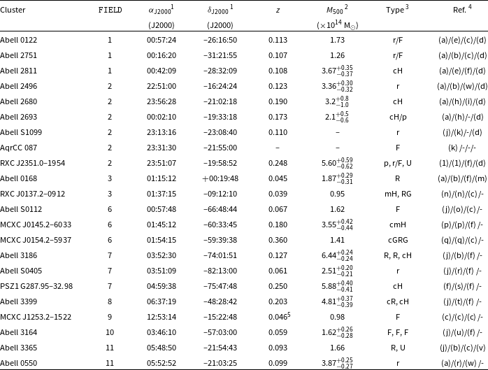
1 Coordinates are shown in units of hours, minutes, seconds, and degrees, arcminutes, arcseconds.
2 Mass within
 $R_{500}$
, the radius within which the mean density of the cluster is 500 times the critical density of the Universe.
$R_{500}$
, the radius within which the mean density of the cluster is 500 times the critical density of the Universe.
3 Detected diffuse source types (either as reported in the literature or as determined in this work): relic (R), halo (H), mini-halo (mH), remnant radio galaxy/AGN (r), miscellaneous fossil plasma/re-accelerated fossil plasma source (e.g. phoenix) (F), candidate (c), point source (p), normal radio galaxy (RG), giant radio galaxy (GRG), unclassified (U).
4 References for position/z/
 $M_{500}$
/previously detected diffuse emission: (a) Abell (Reference Abell1958). (b) Struble & Rood (Reference Struble and Rood1999). (c) (
$M_{500}$
/previously detected diffuse emission: (a) Abell (Reference Abell1958). (b) Struble & Rood (Reference Struble and Rood1999). (c) (
 $M_{{X},500}$
) Piffaretti et al. (Reference Piffaretti, Arnaud, Pratt, Pointecouteau and Melin2011). (d) Duchesne et al. (Reference Duchesne, Johnston-Hollitt, Offringa, Pratt, Zheng and Dehghan2021b). (e) Zaritsky et al. (Reference Zaritsky and Gonzalez2006). (f) (
$M_{{X},500}$
) Piffaretti et al. (Reference Piffaretti, Arnaud, Pratt, Pointecouteau and Melin2011). (d) Duchesne et al. (Reference Duchesne, Johnston-Hollitt, Offringa, Pratt, Zheng and Dehghan2021b). (e) Zaritsky et al. (Reference Zaritsky and Gonzalez2006). (f) (
 $M_{{SZ},500}$
) Planck Collaboration et al. (2015). (g) Cavagnolo et al. (Reference Cavagnolo, Donahue, Voit and Sun2008). (h) Coziol et al. (Reference Coziol, Andernach, Caretta, Alamo-MartÍnez and Tago2009). (i) Wen & Han (Reference Wen and Han2015). (j) Abell et al. (1989). (k) Caretta et al. (Reference Caretta, Maia, Kawasaki and Willmer2002). (l) Chon & Böhringer (Reference Chon and Böhringer2012). (m) Dwarakanath et al. (Reference Dwarakanath, Parekh, Kale and George2018). (n) Cruddace et al. (Reference Cruddace2002). (o) Garilli et al. (Reference Garilli, Maccagni and Tarenghi1993). (p) Schwope et al. (Reference Schwope2000). (q) Vikhlinin et al. (Reference Vikhlinin, McNamara, Forman, Jones, Quintana and Hornstrup1998). (r) De Grandi et al. (Reference De Grandi1999). (s) Planck Collaboration et al. (Reference Planck2014). (t) Böhringer et al. (Reference Böhringer2004). (u) Fleenor et al. (Reference Fleenor, Rose, Christiansen, Johnston-Hollitt, Hunstead, Drinkwater and Saunders2006). (v) van Weeren et al. (Reference van Weeren, Brüggen, Röttgering, Hoeft, Nuza and Intema2011). (w) Planck Collaboration et al. (2016).
$M_{{SZ},500}$
) Planck Collaboration et al. (2015). (g) Cavagnolo et al. (Reference Cavagnolo, Donahue, Voit and Sun2008). (h) Coziol et al. (Reference Coziol, Andernach, Caretta, Alamo-MartÍnez and Tago2009). (i) Wen & Han (Reference Wen and Han2015). (j) Abell et al. (1989). (k) Caretta et al. (Reference Caretta, Maia, Kawasaki and Willmer2002). (l) Chon & Böhringer (Reference Chon and Böhringer2012). (m) Dwarakanath et al. (Reference Dwarakanath, Parekh, Kale and George2018). (n) Cruddace et al. (Reference Cruddace2002). (o) Garilli et al. (Reference Garilli, Maccagni and Tarenghi1993). (p) Schwope et al. (Reference Schwope2000). (q) Vikhlinin et al. (Reference Vikhlinin, McNamara, Forman, Jones, Quintana and Hornstrup1998). (r) De Grandi et al. (Reference De Grandi1999). (s) Planck Collaboration et al. (Reference Planck2014). (t) Böhringer et al. (Reference Böhringer2004). (u) Fleenor et al. (Reference Fleenor, Rose, Christiansen, Johnston-Hollitt, Hunstead, Drinkwater and Saunders2006). (v) van Weeren et al. (Reference van Weeren, Brüggen, Röttgering, Hoeft, Nuza and Intema2011). (w) Planck Collaboration et al. (2016).
5 A second system (Abell 1631) is detected at
 $z=0.014$
(Coziol et al. Reference Coziol, Andernach, Caretta, Alamo-MartÍnez and Tago2009)—see cluster entry in Section 3.1 for details.
$z=0.014$
(Coziol et al. Reference Coziol, Andernach, Caretta, Alamo-MartÍnez and Tago2009)—see cluster entry in Section 3.1 for details.
The sky coverage of the MWA-2 diffuse source follow-up survey, with named fields labelled and cluster targets reported in this work noted as blue ‘x’ marks. Actual MWA-2 pointings at 154 MHz are shown as transparent black circles, indicating relative sensitivity of fields. While no sources from either FIELD4 or FIELD5 are reported in this work (as discussed in the text) we show their locations for completeness.
2.2. Observations with the MWA-2
For all fields, we observed a range of frequencies, mirroring the GLEAM survey frequency selections: 30-MHz instantaneous bandwidth observations centred on 88, 118, 154, 185, and 216 MHz. Observations are performed in the MWA-standard ‘snapshot’ observing mode, with 2-min drift-scan snapshots. Each snapshot is calibrated and imaged independently prior to stacking/mosaicking.
Processing of the MWA-2 data follow the recipe described in detail by Duchesne et al. (Reference Duchesne, Johnston-Hollitt, Zhu, Wayth and Line2020) making use of the purpose-built Phase II Pipeline (piip Footnote d ) with constituent software which will be briefly described. Individual snapshots are retrieved from the Pawsey Supercomputing CentreFootnote e archive using the MWA component of the All-Sky Virtual ObservatoryFootnote f which performs general pre-processing and initial RFI flagging with AOFlagger Footnote g (Offringa et al. Reference Offringa2015). After snapshots are retrieved and pre-processed, they are calibrated using an implementation of the Mitchcal algorithm (Offringa et al. Reference Offringa2016) using a global sky model as described in Duchesne et al. (Reference Duchesne, Johnston-Hollitt, Zhu, Wayth and Line2020). Imaging per snapshot is performed with WSClean Footnote h (version 2.9.0; Offringa et al. Reference Offringa2014; Offringa & Smirnov Reference Offringa and Smirnov2017) using multi-scale CLEANing.
Final images are corrected for astrometry using fits_warp.py (version 2.0; Hancock et al. Reference Hancock, Trott and Hurley-Walker2018) and the flux scale is set using flux_warp
Footnote
i
(version 1.14). Both of these tools take an input sky model generated by cross-matching and spectral modelling of GLEAM, the NRAOFootnote
j
VLAFootnote
k
Sky Survey (NVSS; Condon et al. Reference Condon, Cotton, Greisen, Yin, Perley, Taylor and Broderick1998) and/or the Sydney University Molonglo Sky Survey (SUMSS; Bock et al. Reference Bock, Large and Sadler1999; Mauch et al. Reference Mauch, Murphy, Buttery, Curran, Hunstead, Piestrzynski, Robertson and Sadler2003; Murphy et al. Reference Murphy, Mauch, Green, Hunstead, Piestrzynska, Kels and Sztajer2007) using the Positional Update and Matching Algorithm (PUMA; Line et al. Reference Line, Webster, Pindor, Mitchell and Trott2017). This sky model is in turn cross-matched to point sources in the snapshot image catalogues to calculate astrometric offsets and flux density discrepancies. Corrections are applied over the snapshots via interpolation between cross-matched sources. Finally, snapshot images are stacked to create mosaics as described in Duchesne et al. (Reference Duchesne, Johnston-Hollitt, Zhu, Wayth and Line2020). Flux density scale uncertainties are derived by comparing point source flux densities with the PUMA-generated sky model finding
 $\sim\!2$
–10% standard deviation across the observed fields and frequencies. An additional 8% per cent is added in quadrature as inherited from the GLEAM survey, which dominates the flux densities in the sky model. Bulk image details are presented in Table 2.
$\sim\!2$
–10% standard deviation across the observed fields and frequencies. An additional 8% per cent is added in quadrature as inherited from the GLEAM survey, which dominates the flux densities in the sky model. Bulk image details are presented in Table 2.
MWA-2 and ASKAP observation and image details. Note due to the large number of separate images produced, there is a large range of values and here we report the minimum and maximum values for each quantity for each field. Exact PSF values used in measurements are provided as part of the online table described in Appendix B.
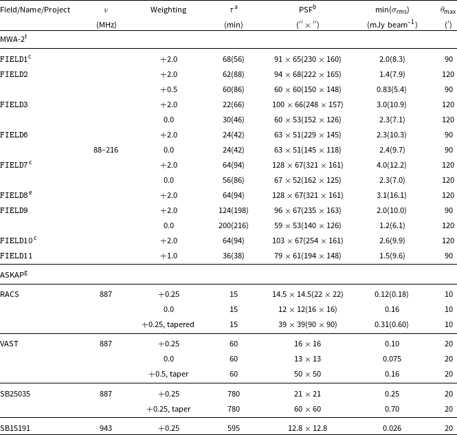
a Range of total stacked times for MWA snapshots, though note that effective sensitivity varies over the map due to mixed primary beam pointings/patterns. For ASKAP observations, this is simply integration time.
b Range of major and minor axes of the PSF at the centre of the stacked images for the various images/frequencies.
c Alternate imaging published in Duchesne et al. (Reference Duchesne, Johnston-Hollitt and Wilber2021c).
d FIELD7 and FIELD10 have significant enough overlap that they are combined for a joint FIELD7+FIELD10 for increased sensitivity, though two individual maps are made centred on each field.
e Alternate imaging for this field published in Brüggen et al. (Reference Brüggen2021) and Duchesne et al. (Reference Duchesne, Johnston-Hollitt and Wilber2021c).
f For MWA-2 observations, all fields are observed at 88, 118, 154, 185, and 216 MHz, and in general resolution increases with frequency, sensitivity peaks at 154 MHz except for zenith fields where sensitivity peaks at 216 MHz, and integration time varies across frequencies due to difference in data lost to ionospheric problems or other calibration problems. As discussed in the text, FIELD4 and FIELD5 are not presented in this work.
g All ASKAP data are re-imaged.
The ‘extended’ configuration of the MWA was created with the same number of tiles (i.e. 128) as the Phase I MWA due to limitations of the current correlator. Creating the longer baselines of the MWA-2 therefore required removing a significant number of short baselines, reducing the sensitivity to larger angular scales compared to the Phase I MWA (Hodgson et al. Reference Hodgson, Johnston-Hollitt, McKinley, Vernstrom and Vacca2020). While the loss of sensitivity for this work is comparatively minimal, we still find that images weighted with a ‘Briggs’ (Briggs Reference Briggs1995) robust parameter of
 $\lesssim\!+0.5$
begin to significantly lose large-scale flux. Therefore, for flux density measurements we create at set of robust
$\lesssim\!+0.5$
begin to significantly lose large-scale flux. Therefore, for flux density measurements we create at set of robust
 $+2.0$
images for all fields except FIELD11 for which we use robust
$+2.0$
images for all fields except FIELD11 for which we use robust
 $+1.0$
Footnote
l
. We also create images at 0.0 and
$+1.0$
Footnote
l
. We also create images at 0.0 and
 $+0.5$
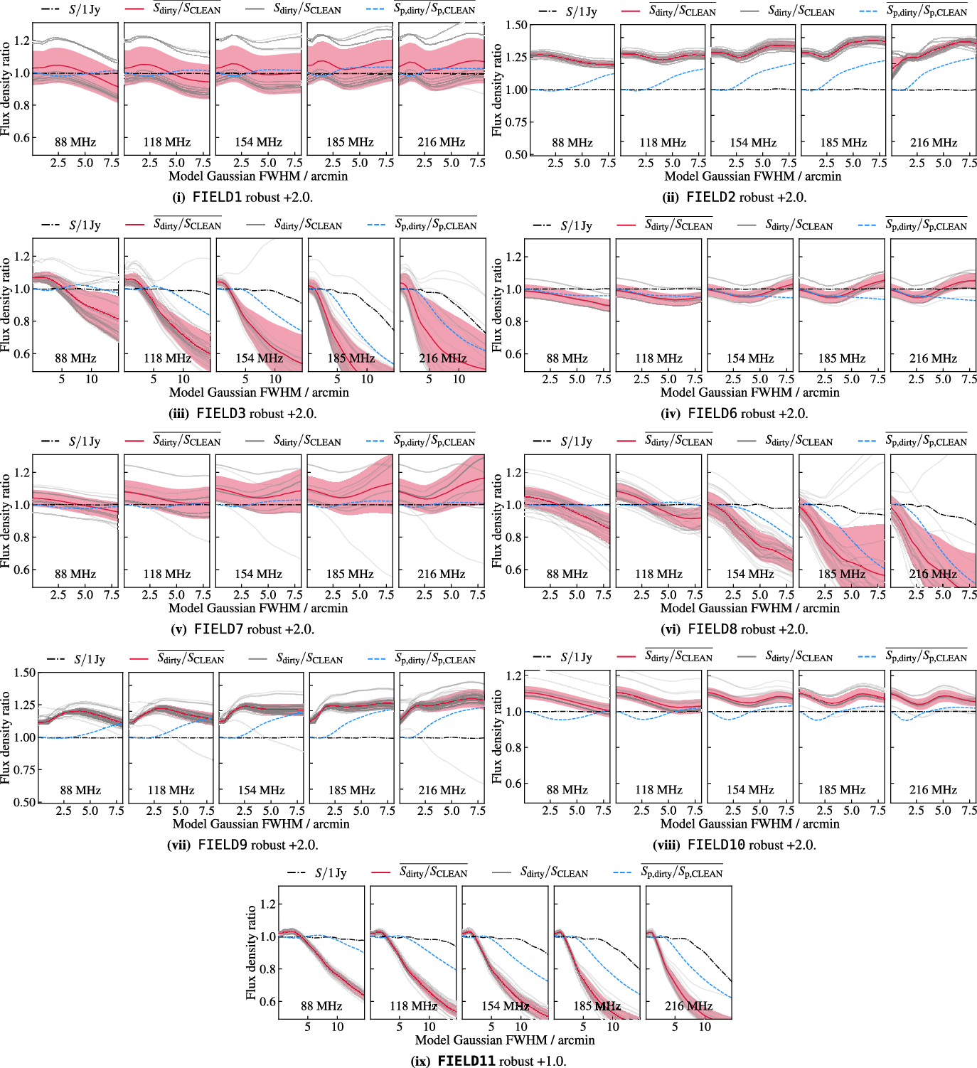
to leverage the resolution increase, though these images are typically used for morphological reference only, unless otherwise noted. Figure 27(i)–(ix) in app:dirty highlight the ‘dirty flux’ bias introduced due to the snapshot stacking method used which is corrected as described in Section 2.1.2 of Duchesne et al. (Reference Duchesne, Johnston-Hollitt and Wilber2021c). Final imaging details are collected in Table 2. Note FIELD5 was published in Duchesne et al. (Reference Duchesne, Johnston-Hollitt, Zhu, Wayth and Line2020) and no further sources have been detected in that field so is not discussed here. FIELD4 suffered from significant sidelobe contamination from Cygnus A with the 185- and 216-MHz bands rendered unusable and will not be considered until future observations can be made when Cygnus A is not present in the primary beam sidelobeFootnote
m
.
$+0.5$
to leverage the resolution increase, though these images are typically used for morphological reference only, unless otherwise noted. Figure 27(i)–(ix) in app:dirty highlight the ‘dirty flux’ bias introduced due to the snapshot stacking method used which is corrected as described in Section 2.1.2 of Duchesne et al. (Reference Duchesne, Johnston-Hollitt and Wilber2021c). Final imaging details are collected in Table 2. Note FIELD5 was published in Duchesne et al. (Reference Duchesne, Johnston-Hollitt, Zhu, Wayth and Line2020) and no further sources have been detected in that field so is not discussed here. FIELD4 suffered from significant sidelobe contamination from Cygnus A with the 185- and 216-MHz bands rendered unusable and will not be considered until future observations can be made when Cygnus A is not present in the primary beam sidelobeFootnote
m
.
2.3. ASKAP survey data
2.3.1. Data and re-processing
The Rapid ASKAP Continuum Survey (McConnell et al. Reference McConnell2020) at 887 MHz covers the entire sky below
 $\delta_{{\rm{J}}2000} \sim +30^\circ$
and covers all clusters in our sample. The survey has a resolution of
$\delta_{{\rm{J}}2000} \sim +30^\circ$
and covers all clusters in our sample. The survey has a resolution of
 $\sim\!15$
arcsec and noise of
$\sim\!15$
arcsec and noise of
 $\sim\!250$
–400
$\sim\!250$
–400
 $\mu$
Jy beam−1. This imaging is sufficient in most cases to detect discrete source populations within the emission regions in the MWA data. ASKAP data (images and calibrated visibilities) are publicly available through the CSIROFootnote
n
ASKAP Science Data Archive (CASDA; Chapman et al. Reference Chapman, Dempsey, Miller, Heywood, Pritchard, Sangster, Whiting and Dart2017). RACS data products are available under project AS110 (Hotan et al. Reference Hotan, Whiting, Huynh and Moss2020a).
$\mu$
Jy beam−1. This imaging is sufficient in most cases to detect discrete source populations within the emission regions in the MWA data. ASKAP data (images and calibrated visibilities) are publicly available through the CSIROFootnote
n
ASKAP Science Data Archive (CASDA; Chapman et al. Reference Chapman, Dempsey, Miller, Heywood, Pritchard, Sangster, Whiting and Dart2017). RACS data products are available under project AS110 (Hotan et al. Reference Hotan, Whiting, Huynh and Moss2020a).
We are able to obtain slightly higher sensitivity in the RACS images by re-imaging with a robust
 $+0.25$
weighting using WSClean which has the added benefit of enhancing any detected diffuse emission with only a minor loss in resolution. For clusters where discrete sources are strong enough to be subtracted using a suitable u,v cut (ranging from 1 700–3 000
$+0.25$
weighting using WSClean which has the added benefit of enhancing any detected diffuse emission with only a minor loss in resolution. For clusters where discrete sources are strong enough to be subtracted using a suitable u,v cut (ranging from 1 700–3 000
 $\lambda$
, additionally see Knowles et al. Reference Knowles2021 for some discussion of this problem), we subtract discrete sources and re-image with additional tapering—dependent on the scale of the emission—at a robust
$\lambda$
, additionally see Knowles et al. Reference Knowles2021 for some discussion of this problem), we subtract discrete sources and re-image with additional tapering—dependent on the scale of the emission—at a robust
 $+0.25$
image weighting. For a selection of observations where point sources are either too faint or non-existent, a low-resolution image is made without additional subtraction and intervening source contributions (if any) are subtracted from the flux density measurements. As a quick quality assurance check, we compare any re-processed maps to the RACS survey images and find no significant discrepancies in astrometry or flux scale.
$+0.25$
image weighting. For a selection of observations where point sources are either too faint or non-existent, a low-resolution image is made without additional subtraction and intervening source contributions (if any) are subtracted from the flux density measurements. As a quick quality assurance check, we compare any re-processed maps to the RACS survey images and find no significant discrepancies in astrometry or flux scale.
Two clusters in our sample also benefit from being within archival ASKAP observations performed for the ASKAP survey for Variability And Slow Transients (VAST; Murphy et al. Reference Murphy2013) under pilot project AS107 (Murphy et al. Reference Murphy2020). The set up for these observations is similar to RACS, except they have 5–6
 $\sim\!15$
min identical pointings which we combine and image as above. These data have some overlap in u,v coverage, so the additional u,v coverage is typically only equivalent to 2–3 additional 15-min observations. Source-subtraction is done in the combined visibilities and flux densities of points sources are equivalent to within a few per cent of RACS data at the location of the VAST observations.
$\sim\!15$
min identical pointings which we combine and image as above. These data have some overlap in u,v coverage, so the additional u,v coverage is typically only equivalent to 2–3 additional 15-min observations. Source-subtraction is done in the combined visibilities and flux densities of points sources are equivalent to within a few per cent of RACS data at the location of the VAST observations.
Abell 0122 features at the centre of a beam in a deep observation, SB25035 (Murphy et al. Reference Murphy, Lenc, Whiting, Huynh and Hotan2019)Footnote o . These data are processed identically to images presented of Abell 0141 by Duchesne et al. (Reference Duchesne, Johnston-Hollitt and Wilber2021c) and no flux scale discrepancy is observed. Due to the smaller size of the emission, no low-resolution image is made.
Finally, a single cluster, Abell 3186, is present outside of the full width at half maximum (FWHM) of some beams in a deep, 12-h observation near the Large Magellanic Cloud (SB25035; Hotan et al. Reference Hotan, McConnell, Whiting and Huynh2020b). As the primary beam is not well modelled by a simple 2-d Gaussian
 $\sim\!2$
deg away from the beam centre, we instead cross-match sources in the image to a catalogue derived from the RACS image in the region, and create a pseudo primary beam correction using flux_warp with a linear radial basis function interpolation scheme. This results in flux densities of the surrounding point sources that do not different by more than
$\sim\!2$
deg away from the beam centre, we instead cross-match sources in the image to a catalogue derived from the RACS image in the region, and create a pseudo primary beam correction using flux_warp with a linear radial basis function interpolation scheme. This results in flux densities of the surrounding point sources that do not different by more than
 $\sim\!10$
% from RACS. While the point source sensitivity of this image is comparable to the 15-min RACS image, the inner u,v sampling is denser due to the longer synthesis rotation allowing better recovery of extended emission.
$\sim\!10$
% from RACS. While the point source sensitivity of this image is comparable to the 15-min RACS image, the inner u,v sampling is denser due to the longer synthesis rotation allowing better recovery of extended emission.
While the deep ASKAP observations have a well-sampled u,v plane, as discussed by McConnell et al. (Reference McConnell2020), the short
 $\sim\!15$
-min observations performed for RACS do not allow significant sampling of the inner u,v plane due to lack of significant Earth-rotation synthesis (see e.g. their Figure 4 for an example of the u,v coverage, and see e.g. Figure 2 from Duchesne et al. Reference Duchesne, Johnston-Hollitt, Bartalucci, Hodgson and Pratt2021a for an example of the u,v coverage for a 10-h ASKAP observation). While in principle structures up to
$\sim\!15$
-min observations performed for RACS do not allow significant sampling of the inner u,v plane due to lack of significant Earth-rotation synthesis (see e.g. their Figure 4 for an example of the u,v coverage, and see e.g. Figure 2 from Duchesne et al. Reference Duchesne, Johnston-Hollitt, Bartalucci, Hodgson and Pratt2021a for an example of the u,v coverage for a 10-h ASKAP observation). While in principle structures up to
 $\sim\!10$
arcmin can be recovered, the lower sensitivity at this large angular scale only allows the brightest large-scale objects to be recovered fully. Generally the sources we will discuss in this work are sufficiently small to not be heavily affected (with some exceptions, noted where appropriate) and measurements typically agree with spectra obtained from MWA-2 data alone.
$\sim\!10$
arcmin can be recovered, the lower sensitivity at this large angular scale only allows the brightest large-scale objects to be recovered fully. Generally the sources we will discuss in this work are sufficiently small to not be heavily affected (with some exceptions, noted where appropriate) and measurements typically agree with spectra obtained from MWA-2 data alone.
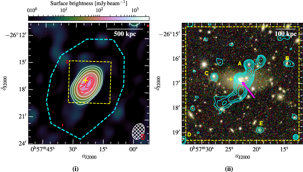
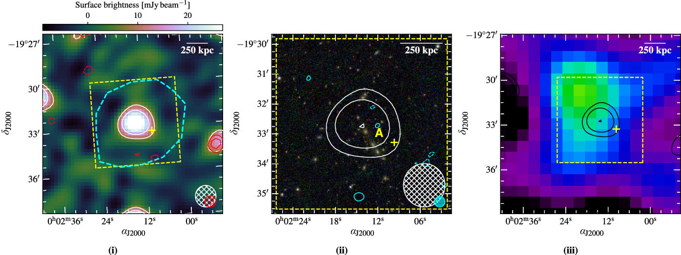
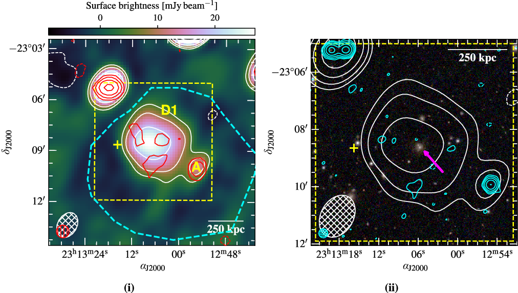
Abell 0122. (i). Background: MWA-2, 185 MHz, robust
 $+2.0$
image. (ii). Background: RGB DES image (i, r, g). Where relevant, the white contours are from the background image in (i), in levels of
$+2.0$
image. (ii). Background: RGB DES image (i, r, g). Where relevant, the white contours are from the background image in (i), in levels of
 $[\pm 3, 6, 12, 24, 48] \times \sigma_{\rm{rms}}$
(
$[\pm 3, 6, 12, 24, 48] \times \sigma_{\rm{rms}}$
(
 $\sigma_{\rm{rms}} = 2.5$
mJy beam−1). Red contours: TGSS image, in levels of
$\sigma_{\rm{rms}} = 2.5$
mJy beam−1). Red contours: TGSS image, in levels of
 $[\pm 3, 6, 12, 24, 48] \times \sigma_{\rm{rms}}$
(
$[\pm 3, 6, 12, 24, 48] \times \sigma_{\rm{rms}}$
(
 $\sigma_{\rm{rms}} = 4.5$
mJy beam−1. Cyan contours: deep ASKAP robust
$\sigma_{\rm{rms}} = 4.5$
mJy beam−1. Cyan contours: deep ASKAP robust
 $+0.25$
image, in levels of
$+0.25$
image, in levels of
 $[\pm 3, 6, 12, 24, 48] \times \sigma_{\rm{rms}}$
(
$[\pm 3, 6, 12, 24, 48] \times \sigma_{\rm{rms}}$
(
 $\sigma_{\rm{rms}} = 0.026$
mJy beam−1). The dashed, yellow box is identical in both panels. The ellipses in the lower corners correspond to the respective beams. Sources discussed in the text are labelled. Linear scale bars are at the redshift of the cluster. The magenta arrow points towards the brightest cluster galaxy (BCG). The yellow cross indicates the reported cluster centre.
$\sigma_{\rm{rms}} = 0.026$
mJy beam−1). The dashed, yellow box is identical in both panels. The ellipses in the lower corners correspond to the respective beams. Sources discussed in the text are labelled. Linear scale bars are at the redshift of the cluster. The magenta arrow points towards the brightest cluster galaxy (BCG). The yellow cross indicates the reported cluster centre.
General ASKAP imaging details are presented in Table 2, and as with the MWA-2 data a range of imaging properties are reported for the various RACS images made. For non-RACS images, we report the exact properties.
2.4. Spectral properties
2.4.1. Intervening source contributions
Due to the low resolution of the MWA (even in its extended configuration) we have to carefully consider contamination from confusing sources. The two main scenarios we consider are case (1) brighter sources blended with the diffuse emission, and/or case (2) faint underlying/intervening sources within the detected MWA emission. Case (1) is simple in the sense that bright sources are easily detected with low resolution surveys such as the NVSS or SUMSS, both with
 $\sim\!45$
arcsec resolution, or the TIFRFootnote
p
GMRTFootnote
q
Sky Survey (TGSS; Intema et al. Reference Intema, Jagannathan, Mooley and Frail2017) with
$\sim\!45$
arcsec resolution, or the TIFRFootnote
p
GMRTFootnote
q
Sky Survey (TGSS; Intema et al. Reference Intema, Jagannathan, Mooley and Frail2017) with
 $\sim\!25$
arcsec resolution. The RACS survey data are suitable for this purpose also, and the MWA-2 and GLEAM data can also be useful in this case.
$\sim\!25$
arcsec resolution. The RACS survey data are suitable for this purpose also, and the MWA-2 and GLEAM data can also be useful in this case.
In case (1), we can generally detect these brighter sources across multiple frequencies and model their spectra to remove their contribution in the MWA images, fitting a normal power law model of the form
 $${S_{v,{\rm{discrete}}}} = {S_{0,{\rm{discrete}}}}{({\rm{v}}/{v_0})^\alpha },$$
for extrapolation to
 $S_{v,{{\rm{discrete}}}}$
from a measured flux density
$S_{v,{{\rm{discrete}}}}$
from a measured flux density
 $S_{0,{{\rm{discrete}}}}$
. For sources with only two measurements we derive a two-point spectral index rearranging Eq. (1). We did not encounter any intervening discrete sources that required more complex spectral energy distribution (SED) modelling. Uncertainty in the initial discrete source measurements and spectral index are propagated to the extrapolated value.
$S_{0,{{\rm{discrete}}}}$
. For sources with only two measurements we derive a two-point spectral index rearranging Eq. (1). We did not encounter any intervening discrete sources that required more complex spectral energy distribution (SED) modelling. Uncertainty in the initial discrete source measurements and spectral index are propagated to the extrapolated value.
Case (2) typically involves sources that are only detected in RACS or other higher-resolution data due to the relative sensitivities of the various low-resolution surveys. If multiple data sets are available, we model the SED as above to extrapolate discrete source flux densities at MWA frequencies. For sources without spectral coverage, we assume a spectral index. Typically this is assumed to be
 $\left\langle \alpha \right\rangle = - 0.7$
, though for some sources we note a non-detection in some MWA-2 bands/TGSS imply flatter spectra and modify the assumed spectral index appropriately. We use a range of
$\left\langle \alpha \right\rangle = - 0.7$
, though for some sources we note a non-detection in some MWA-2 bands/TGSS imply flatter spectra and modify the assumed spectral index appropriately. We use a range of
 $\alpha$
to estimate additional uncertainty in the unknown spectral index, via:
$\alpha$
to estimate additional uncertainty in the unknown spectral index, via:
 $${S_{v,{\rm{discrete}}}} = {S_{0,{\rm{discrete}}}}{u^{\left\langle \alpha \right\rangle }} \pm {\sigma _{{S_{v,{\rm{discrete}}}}}}\quad [{\rm{Jy}}],$$
and
 \begin{equation} \sigma_{S_{v,{\rm{discrete}}}} = S_{0,{\rm{discrete}}}\| u^{\alpha_{min}} - u^{\alpha_{max}} \| \quad [{{\rm{Jy}}}] \, ,\end{equation}
where
 $\alpha_{\rm{min}} = -1.0$
and
$\alpha_{\rm{min}} = -1.0$
and
 $\alpha_{\rm{max}} = -0.5$
, typically, though may be chosen to reflect limits on point source contributions as seen in TGSS or MWA images. For each source, we report the total confusing flux density contributions that are subtracted, along with associated uncertainty in the online table (see Appendix B for details of the online table).
$\alpha_{\rm{max}} = -0.5$
, typically, though may be chosen to reflect limits on point source contributions as seen in TGSS or MWA images. For each source, we report the total confusing flux density contributions that are subtracted, along with associated uncertainty in the online table (see Appendix B for details of the online table).
2.4.2. Flux density measurements
Flux density measurements are predominantly made using the lower-resolution robust
 $+2.0$
/
$+2.0$
/
 $+1.0$
images along with the GLEAM 200-MHz image and select ASKAP images. For certain sources/fields MWA-2 robust
$+1.0$
images along with the GLEAM 200-MHz image and select ASKAP images. For certain sources/fields MWA-2 robust
 $0.0$
/
$0.0$
/
 $+0.5$
images are used to maximise the signal-to-noise ratio (SNR) for smaller sources. Flux density measurements are performed using in-house code, fluxtools.py
Footnote
r
by integration over a bespoke polygon region enclosing the source at all frequencies. This means the region is large enough to enclose the emission seen in the lowest-resolution images (usually the 88-MHz maps).
$+0.5$
images are used to maximise the signal-to-noise ratio (SNR) for smaller sources. Flux density measurements are performed using in-house code, fluxtools.py
Footnote
r
by integration over a bespoke polygon region enclosing the source at all frequencies. This means the region is large enough to enclose the emission seen in the lowest-resolution images (usually the 88-MHz maps).
As the MWA-2 images are only CLEANed to the noise level in the individual 2-min snapshots, additional consideration is made for the un-deconvolved/‘dirty’ flux density contribution in the final stacked images. As described in Duchesne et al. (Reference Duchesne, Johnston-Hollitt and Wilber2021c), the measurement of flux density may not be consistent before and after CLEANing, and the measurement process has the added complexity of normalising the residual, ‘dirty’ flux density to the CLEAN flux density. Figure 27(i)–(ix) in Appendix D show this effect for simulated Gaussian sources of varying size, highlighting the dependence on source size.
Flux density measurements,
 $S_v$
, can therefore be described by
$S_v$
, can therefore be described by
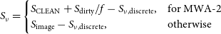 \begin{equation} S_v = \begin{cases} S_{\rm{CLEAN}} + S_{\rm{dirty}}/f - S_{v,{\rm{discrete}}}, & \text{for MWA -2} \\ S_{\rm{image}} - S_{v,{\rm{discrete}}}, & {\rm{otherwise}} \\ \end{cases}\end{equation}
where
 $S_{\rm{CLEAN}}$
is the contribution from the stacked CLEAN component model,
$S_{\rm{CLEAN}}$
is the contribution from the stacked CLEAN component model,
 $S_{\rm{dirty}}$
is contribution from the stacked residual map, f is the model ratio
$S_{\rm{dirty}}$
is contribution from the stacked residual map, f is the model ratio
 $\overline{S_{\rm{dirty}}/S_{\rm{CLEAN}}}$
determined from simulated Gaussian sources, dependent on source size (Figure 27(i)–(ix)), and
$\overline{S_{\rm{dirty}}/S_{\rm{CLEAN}}}$
determined from simulated Gaussian sources, dependent on source size (Figure 27(i)–(ix)), and
 $S_{\rm{discrete}}$
is the contribution from intervening discrete sources. For the non-MWA-2 images,
$S_{\rm{discrete}}$
is the contribution from intervening discrete sources. For the non-MWA-2 images,
 $S_{\rm{image}}$
is measured directly from the restored images.
$S_{\rm{image}}$
is measured directly from the restored images.
The uncertainty on the flux density measurement,
 $\sigma_{S_v}$
, is estimated as the quadrature sum of the various sources of uncertainty following
$\sigma_{S_v}$
, is estimated as the quadrature sum of the various sources of uncertainty following
 $${\sigma _{{S_v}}} = {[{({\sigma _{\rm{scale}}}{S_v})^2} + {({\sigma _{\rm{discrete}}})^2} + {N_{\rm{beam}}}{({\sigma _{\rm{rms}}})^2} + {({\sigma _{{\rm{std}},f}}{S_{\rm{dirty}}})^2}]^{0.5}},$$
where
 $\sigma_{\rm{scale}}$
is the flux scale uncertainty for the image,
$\sigma_{\rm{scale}}$
is the flux scale uncertainty for the image,
 $\sigma_{{\rm{std}},f}$
is the standard deviation in values of f over all snapshots for a given stacked MWA-2 image,
$\sigma_{{\rm{std}},f}$
is the standard deviation in values of f over all snapshots for a given stacked MWA-2 image,
 $\sigma_{\rm{discrete}}$
is the uncertainty in the subtracted discrete source contribution, and
$\sigma_{\rm{discrete}}$
is the uncertainty in the subtracted discrete source contribution, and
 $N_{\rm{beam}}$
is the number of independent restoring beams that cover the polygon region used for measurement. Typically the
$N_{\rm{beam}}$
is the number of independent restoring beams that cover the polygon region used for measurement. Typically the
 $\sigma_{\rm{scale}}$
term dominates, as this is
$\sigma_{\rm{scale}}$
term dominates, as this is
 $\sim\!8$
–10% for all MWA and ASKAP images. The
$\sim\!8$
–10% for all MWA and ASKAP images. The
 ${({\sigma _{{\rm{std}},f}}{S_{\rm{dirty}}})^2}$
term is only included for MWA-2 images.
${({\sigma _{{\rm{std}},f}}{S_{\rm{dirty}}})^2}$
term is only included for MWA-2 images.
2.4.3. Spectra and spectral indices
The measured flux densities and uncertainties are used for modelling the integrated spectra within the observed frequency range. For sources with only MWA-2 data, we find a normal power law (as in Eq. 1) describes the data sufficiently wellFootnote s and provides a spectral index for the source. For sources where additional flux density measurements are available, we find a mixture of power law and curved power law models can be used to describe the observed spectra. We use a generic curved power law model of the form (Duffy & Blundell Reference Duffy and Blundell2012)
 $${S_v} \propto {v^\alpha }\exp [q{(\ln v)^{\rm{2}}}],$$
where q gives an indication of curvature in the spectrum. For each source we provide a fitted power law model or a curved power law model if appropriate, with the combined MWA-2 and supplementary data. An additional power law model is fit solely to the MWA-2 measurements providing a low-frequency spectral index. Model parameters and uncertainties are estimated via non-linear weighted least-squares curve fitting with the Levenberg–Marquardt algorithm and we report
 $1\sigma$
uncertainties.
$1\sigma$
uncertainties.
2.5. Archival X-ray observations
X-ray datasets used in this work were taken using the XMM-Newton European Photon Imaging Camera (EPIC, Turner et al. Reference Turner2001 and Strüder et al. Reference Strüder2001) except for the observation of Abell 3399 which was taken using the Advanced CCD Imaging Spectrometer (ACIS, Garmire et al. Reference Garmire, Bautz, Ford, Nousek, Ricker George and Tananbaum2003) on board of the Chandra observatory. The details of data reduction can be found in the Appendix A of Bartalucci et al. (Reference Bartalucci2017). We used the same reduction and cleaning procedures but updated versions of the Chandra and XMM-Newton analysis software CIAO (Fruscione et al. Reference Fruscione2006) ver. 4.11 with CALDB 4.8.5 and SAS (ver. 15.0) with CCF updated up to March 2021, respectively. The useful exposure times after the cleaning procedures and the observations used are reported in Table 3. The datasets were then arranged in data-cubes and corresponding exposure and background maps were calculated as detailed in Bourdin & Mazzotta Reference Bourdin and Mazzotta2008, Bourdin et al. Reference Bourdin, Mazzotta, Markevitch, Giacintucci and Brunetti2013 and Bogdán et al. Reference Bogdán2013. Point sources were detected using the technique described in Bogdán et al. Reference Bogdán2013, visually inspected for false positives or missed sources and then removed from the analysis. Exposure-corrected and background subtracted images are produced in the [0.5–2.5] keV band.
X-ray observation properties.
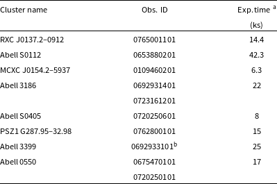
a Exposure time after the cleaning procedures described in Section 2.5.
b Chandra dataset.
2.6. Additional survey data
In addition to the already discussed radio survey images (NVSS, TGSS, SUMSS, and GLEAM), we make use of images from the ROSAT Footnote t All Sky Survey (RASS; Voges et al. Reference Voges1999) for select clusters without deep Chandra or XMM-Newton observations and optical data from the SuperCOSMOS Sky Survey (SSS; Hambly et al. Reference Hambly2001a; Hambly et al. Reference Hambly, Irwin and MacGillivray2001b; Hambly et al. Reference Hambly, Davenhall, Irwin and MacGillivray2001c), the first Pan-STARRSFootnote u survey (PS1; Tonry et al. Reference Tonry2012; Chambers et al. Reference Chambers2016), and the Dark Energy Survey Data Release 2 (DES DR2; Abbott et al. Reference Abbott2018; Morganson et al. Reference Morganson2018; Flaugher et al. Reference Flaugher2015, hereafter DES).
3. Results
3.1. Individual clusters
In this section we will describe the individual clusters ordered by observed field. Individual plots of source SEDs are shown in Appendix C and measurements for cluster sources are provided as an online table described in Appendix B.
3.1.1. FIELD1
Abell 0122 (Figure 2). Reported by D21 as an unclassified steep spectrum source. The source is detected in the MWA-2, TGSS, and deep ASKAP data, shown in Figure 2(i) and Figure 2(ii). The deep ASKAP data show a complex source with additional point source contributions (labelled in Figure 2(ii)) and with contribution from what may be the core of the emission, the brightest cluster galaxy (BCG) (6dF J0057228–261653; Jones et al. Reference Jones2009) indicated by a magenta arrow in Figure 2(ii). The projected extent of the source is
 $\sim\!2.6$
arcmin (corresponding to
$\sim\!2.6$
arcmin (corresponding to
 $\sim\!310$
kpc), including the protrusion to the West of Source A. This is slightly smaller than that reported by D21 due to less source blending. The SED between 88–943 MHz is shown in Figure 26(i), finding curvature between the MWA and ASKAP data after subtraction of the labelled sources, and with a spectral index from 88–216 MHz of
$\sim\!310$
kpc), including the protrusion to the West of Source A. This is slightly smaller than that reported by D21 due to less source blending. The SED between 88–943 MHz is shown in Figure 26(i), finding curvature between the MWA and ASKAP data after subtraction of the labelled sources, and with a spectral index from 88–216 MHz of
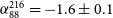 $\alpha_{88}^{216} = -1.6 \pm 0.1$
. We consider this a remnant radio galaxy, likely associated with the BCG, or otherwise fossil plasma originally from the BCG.
$\alpha_{88}^{216} = -1.6 \pm 0.1$
. We consider this a remnant radio galaxy, likely associated with the BCG, or otherwise fossil plasma originally from the BCG.
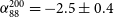
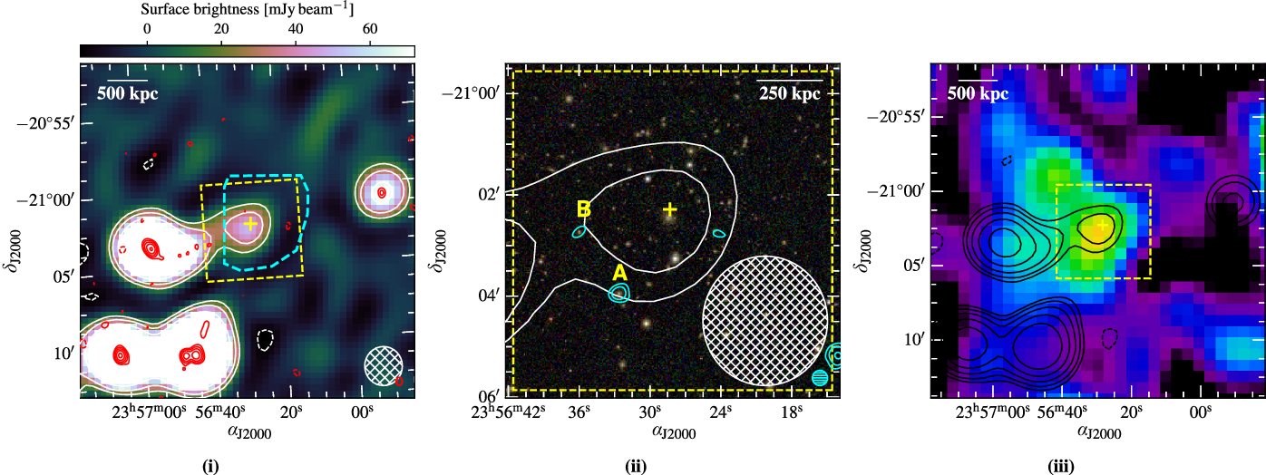
Abell 2751 (Figure 3). D21 report a relic source on the outskirts of Abell 2751 (D1 in Figure 3(i)). We show the MWA-2 and RACS discrete source-subtracted images in Figure 3(i), and the higher-resolution RACS image in Figure 3(ii) showing the embedded compact source labelled B. The largest angular size (LAS) is 4.7 arcmin corresponding to a largest linear size (LLS) of 580 kpc, slightly smaller than that reported by D21 due to the less confused images. Sources A and B are subtracted from MWA-2 measurements, and we subtract the contribution of B from the measurements presented in D21. A plot of the SED between 88–1400 MHz is shown in Figure 26(ii) in app:seds, and we find a well-fit power law distribution with
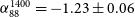 $\alpha_{88}^{1400} = -1.23 \pm 0.06$
, consistent with
$\alpha_{88}^{1400} = -1.23 \pm 0.06$
, consistent with
 $\alpha$
reported by D21. RASS data shown in the Figure 3(iii) indicates the bulk ICM sits to the southwest, with D1 oriented almost perpendicular, which is abnormal for large-scale relics (with the exception of the relic source in MACS J1149.5
$\alpha$
reported by D21. RASS data shown in the Figure 3(iii) indicates the bulk ICM sits to the southwest, with D1 oriented almost perpendicular, which is abnormal for large-scale relics (with the exception of the relic source in MACS J1149.5
 $+$
2223, though the nature of that source is unclear; Bonafede et al. Reference Bonafede2012; Bruno et al. Reference Bruno2021). With no evidence of shocks (and an absence of more sensitive X-ray data) we cannot differentiate from relic or fossil electrons/remnant radio galaxy. The reported cluster centre by Abell et al. (1989) is offset from the RASS X-ray peak by
$+$
2223, though the nature of that source is unclear; Bonafede et al. Reference Bonafede2012; Bruno et al. Reference Bruno2021). With no evidence of shocks (and an absence of more sensitive X-ray data) we cannot differentiate from relic or fossil electrons/remnant radio galaxy. The reported cluster centre by Abell et al. (1989) is offset from the RASS X-ray peak by
 $\sim\!2$
arcmin (
$\sim\!2$
arcmin (
 $\sim\!230$
kpc); the optical concentration of galaxies is also elongated (Duchesne et al. Reference Duchesne, Johnston-Hollitt, Offringa, Pratt, Zheng and Dehghan2021b, see their Figure 15)—we suggest the system is merging based on these observations, and significant shocks may be present in the cluster volume. We consider this an ambiguous fossil source or remnant.
$\sim\!230$
kpc); the optical concentration of galaxies is also elongated (Duchesne et al. Reference Duchesne, Johnston-Hollitt, Offringa, Pratt, Zheng and Dehghan2021b, see their Figure 15)—we suggest the system is merging based on these observations, and significant shocks may be present in the cluster volume. We consider this an ambiguous fossil source or remnant.
Abell 2751. (i). Background: MWA-2, 185 MHz, robust
 $+2.0$
image. (ii). Background: RGB DES image (i, r, g). (iii). Background: Smoothed RASS image. The white contours are as in Figure 2(i) for the background of (i) (
$+2.0$
image. (ii). Background: RGB DES image (i, r, g). (iii). Background: Smoothed RASS image. The white contours are as in Figure 2(i) for the background of (i) (
 $\sigma_{\rm{rms}} = 7$
mJy beam−1), except in (ii) with a single contour at
$\sigma_{\rm{rms}} = 7$
mJy beam−1), except in (ii) with a single contour at
 $3\sigma_{\rm{rms}}$
. Red contours: RACS discrete source-subtracted image,
$3\sigma_{\rm{rms}}$
. Red contours: RACS discrete source-subtracted image,
 $[\pm 3, 6, 12, 24, 48] \times \sigma_{\rm{rms}}$
(
$[\pm 3, 6, 12, 24, 48] \times \sigma_{\rm{rms}}$
(
 $\sigma_{\rm{rms}} = 0.44$
mJy beam−1), except in (ii) with a single contour at
$\sigma_{\rm{rms}} = 0.44$
mJy beam−1), except in (ii) with a single contour at
 $3\sigma_{\rm{rms}}$
. Cyan contours: RACS robust
$3\sigma_{\rm{rms}}$
. Cyan contours: RACS robust
 $+0.25$
image,
$+0.25$
image,
 $[\pm 3, 6, 12, 24, 48] \times \sigma_{\rm{rms}}$
(
$[\pm 3, 6, 12, 24, 48] \times \sigma_{\rm{rms}}$
(
 $\sigma_{\rm{rms}} = 0.2$
mJy beam−1). The yellow circle in (iii) has a 1 Mpc radius centred on the reported cluster coordinates. Other features are as in Figure 2.
$\sigma_{\rm{rms}} = 0.2$
mJy beam−1). The yellow circle in (iii) has a 1 Mpc radius centred on the reported cluster coordinates. Other features are as in Figure 2.
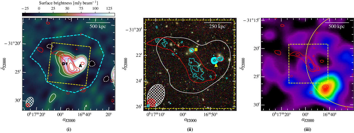
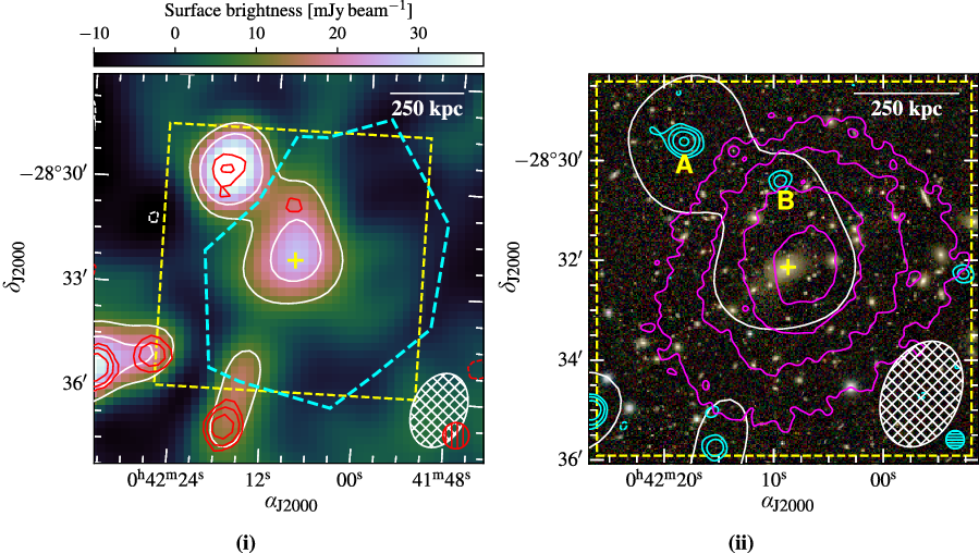
Abell 2811 (Figure 4). Halo/mini-halo candidate reported by D21, detected in MWA-2 data up to 185 MHz, with only partial detection at 216 MHz, and no detection in the RACS data (Figure 4). We measure the integrated flux density across the MWA-2 band, including the 200-MHz GLEAM image, and fit a power law model to the SED (Figure 26(iii)), finding
 $\alpha_{88}^{200} = -2.5 \pm 0.4$
(
$\alpha_{88}^{200} = -2.5 \pm 0.4$
(
 $\alpha_{\text{MWA-2}} = -3.1 \pm 0.5$
for the MWA-2 data only), after subtraction of the contribution of Source B. The 168-MHz measurement reported by D21 is slightly higher than expected due to additional blending with Source A. Additionally, the LAS is
$\alpha_{\text{MWA-2}} = -3.1 \pm 0.5$
for the MWA-2 data only), after subtraction of the contribution of Source B. The 168-MHz measurement reported by D21 is slightly higher than expected due to additional blending with Source A. Additionally, the LAS is
 $2.7$
arcmin (with an LLS of 320 kpc), slightly smaller again due to less blending with Source A. We fit the exposure-corrected and background-subtracted XMM-Newton data presented in D21 with a single-
$2.7$
arcmin (with an LLS of 320 kpc), slightly smaller again due to less blending with Source A. We fit the exposure-corrected and background-subtracted XMM-Newton data presented in D21 with a single-
 $\beta$
model (Cavaliere & Fusco-Femiano Reference Cavaliere and Fusco-Femiano1976), and estimate the X-ray morphological parameters, the centroid shift, w (Poole et al. Reference Poole, Fardal, Babul, McCarthy, Quinn and Wadsley2006), with an outer radius set to
$\beta$
model (Cavaliere & Fusco-Femiano Reference Cavaliere and Fusco-Femiano1976), and estimate the X-ray morphological parameters, the centroid shift, w (Poole et al. Reference Poole, Fardal, Babul, McCarthy, Quinn and Wadsley2006), with an outer radius set to
 $R_{500} = 1.035$
Mpc (Piffaretti et al. Reference Piffaretti, Arnaud, Pratt, Pointecouteau and Melin2011). We find
$R_{500} = 1.035$
Mpc (Piffaretti et al. Reference Piffaretti, Arnaud, Pratt, Pointecouteau and Melin2011). We find
 $w = 0.072R_{500}$
, consistent with disturbed systems (Pratt et al. Reference Pratt, Croston, Arnaud and Böhringer2009). Additionally, the surface brightness concentration,
$w = 0.072R_{500}$
, consistent with disturbed systems (Pratt et al. Reference Pratt, Croston, Arnaud and Böhringer2009). Additionally, the surface brightness concentration,
 $c_{100/500}$
is found to be 0.21, placing it right on the border of merging, halo-hosting clusters (Cassano et al. Reference Cassano, Ettori, Giacintucci, Brunetti, Markevitch, Venturi and Gitti2010). Similarly, the centroid shift within 500 kpc is found to be
$c_{100/500}$
is found to be 0.21, placing it right on the border of merging, halo-hosting clusters (Cassano et al. Reference Cassano, Ettori, Giacintucci, Brunetti, Markevitch, Venturi and Gitti2010). Similarly, the centroid shift within 500 kpc is found to be
 $w_{500} = 0.07$
, placing it outside of halo-hosting quadrant, near Abell 697 which has been reported to host a radio halo (but see also Kempner & Sarazin Reference Kempner and Sarazin2001 Venturi et al. Reference Venturi, Giacintucci, Dallacasa, Cassano, Brunetti, Bardelli and Setti2008) with an ultra-steep spectrum (
$w_{500} = 0.07$
, placing it outside of halo-hosting quadrant, near Abell 697 which has been reported to host a radio halo (but see also Kempner & Sarazin Reference Kempner and Sarazin2001 Venturi et al. Reference Venturi, Giacintucci, Dallacasa, Cassano, Brunetti, Bardelli and Setti2008) with an ultra-steep spectrum (
 $\alpha = -1.5$
; Macario et al. Reference Macario2013), though not as steep as the spectrum for Abell 2811. We also note the concentration parameter,
$\alpha = -1.5$
; Macario et al. Reference Macario2013), though not as steep as the spectrum for Abell 2811. We also note the concentration parameter,
 $c_{40/400} = 0.048$
, is below what is typically seen in CC clusters (Santos et al. Reference Santos, Rosati, Tozzi, Böhringer, Ettori and Bignamini2008, with
$c_{40/400} = 0.048$
, is below what is typically seen in CC clusters (Santos et al. Reference Santos, Rosati, Tozzi, Böhringer, Ettori and Bignamini2008, with
 $c_{40/400} \gtrsim 0.075$
). Many of the properties are consistent with a radio halo, however, such a steep spectrum is rare for radio halos: while we consider this an extreme case of an ultra-steep–spectrum radio halo (USSRH) it may be a fossil plasma source projected onto the cluster centre.
$c_{40/400} \gtrsim 0.075$
). Many of the properties are consistent with a radio halo, however, such a steep spectrum is rare for radio halos: while we consider this an extreme case of an ultra-steep–spectrum radio halo (USSRH) it may be a fossil plasma source projected onto the cluster centre.
Abell 2811. (i). Background: MWA-2, 154 MHz, robust
 $+2.0$
image. (ii). Background: RGB DES image (i, r, g). The white contours are as in Figure 2(i) for the background of (i) (for
$+2.0$
image. (ii). Background: RGB DES image (i, r, g). The white contours are as in Figure 2(i) for the background of (i) (for
 $\sigma_{\rm{rms}} = 3.5$
mJy beam−1). Red contours: NVSS image, in levels of
$\sigma_{\rm{rms}} = 3.5$
mJy beam−1). Red contours: NVSS image, in levels of
 $[\pm 3, 6, 12, 24, 48] \times \sigma_{\rm{rms}}$
(
$[\pm 3, 6, 12, 24, 48] \times \sigma_{\rm{rms}}$
(
 $\sigma_{\rm{rms}} = 0.45$
mJy beam−1. Cyan contours: RACS robust
$\sigma_{\rm{rms}} = 0.45$
mJy beam−1. Cyan contours: RACS robust
 $+0.25$
image, in levels of
$+0.25$
image, in levels of
 $[\pm 3, 6, 12, 24, 48] \times \sigma_{\rm{rms}}$
(
$[\pm 3, 6, 12, 24, 48] \times \sigma_{\rm{rms}}$
(
 $\sigma_{\rm{rms}} = 0.17$
mJy beam−1). Magenta contours: exposure-corrected, background-subtracted XMM-Newton data as presented in D21. Other image features are as in Figure 2.
$\sigma_{\rm{rms}} = 0.17$
mJy beam−1). Magenta contours: exposure-corrected, background-subtracted XMM-Newton data as presented in D21. Other image features are as in Figure 2.
3.1.2. FIELD2
Abell 2496 (Figure 5). Reported by D21 as an unclassifed diffuse cluster source. The MWA-2 and TGSS data in Figure 5(i) show an extended source, with the RACS data in Figure 5(ii) showing a clear double-lobed morphology. A small extension is seen in the RACS data in the direction of the larger extension seen in the TGSS and MWA-2 images, tracing an older plasma component. The angular and linear extend of the source is the same as reported in D21. The overall emission is modelled with a normal power law with
 $\alpha_{88}^{1400} = -1.23 \pm 0.05$
(Figure 26(i)). The PS1 data show possible hosts between the lobes: WISEA J225055.58–162721.0; indicated by a yellow arrow in Figure 5(ii), and WISEA J225054.36-162710.7; indicated by a magenta arrow, neither with known redshifts. No distinct radio core is seen. We suggest this is a remnant radio galaxy.
$\alpha_{88}^{1400} = -1.23 \pm 0.05$
(Figure 26(i)). The PS1 data show possible hosts between the lobes: WISEA J225055.58–162721.0; indicated by a yellow arrow in Figure 5(ii), and WISEA J225054.36-162710.7; indicated by a magenta arrow, neither with known redshifts. No distinct radio core is seen. We suggest this is a remnant radio galaxy.
Abell 2496. (i). Background: MWA-2, 185 MHz, robust
 $+0.5$
image. (ii). Background: RGB PS1 image (i, r, g). The white contours are as in Figure 2(i) for the background of (i) (for
$+0.5$
image. (ii). Background: RGB PS1 image (i, r, g). The white contours are as in Figure 2(i) for the background of (i) (for
 $\sigma_{\rm{rms}} = 1.5$
mJy beam−1). Red contours: TGSS image, in levels of
$\sigma_{\rm{rms}} = 1.5$
mJy beam−1). Red contours: TGSS image, in levels of
 $[\pm 3, 6, 12, 24, 48] \times \sigma_{\rm{rms}}$
(
$[\pm 3, 6, 12, 24, 48] \times \sigma_{\rm{rms}}$
(
 $\sigma_{\rm{rms}} = 4$
mJy beam−1). Cyan contours: RACS robust
$\sigma_{\rm{rms}} = 4$
mJy beam−1). Cyan contours: RACS robust
 $+0.25$
image, in levels of
$+0.25$
image, in levels of
 $[\pm 3, 6, 12, 24, 48] \times \sigma_{\rm{rms}}$
(
$[\pm 3, 6, 12, 24, 48] \times \sigma_{\rm{rms}}$
(
 $\sigma_{\rm{rms}} = 0.23$
mJy beam−1). Other image features are as in Figure 2.
$\sigma_{\rm{rms}} = 0.23$
mJy beam−1). Other image features are as in Figure 2.

Abell 2680 (Figure 6). Reported by D21. Figure 6(i) shows the MWA-2 and TGSS radio data, and Figure 6(ii) the PS1 data with MWA-2 and RACS data overlaid. The LAS of the source is 3.0 arcmin (with an LLS of 580 kpc), slightly larger than reported by D21 and the reduced confusion enables a better estimate of the size. A single compact source is detected within the emission with RACS (Source A) and is subtracted from subsequent flux density measurements. We are only able to provide measurements in the 88-, 118-, and 154-MHz MWA-2 bands as the cluster is towards the edge of FIELD2 with lessened sensitivity in the higher frequency images. We find
 $\alpha_{88}^{200} = -1.7 \pm 0.7$
(Figure 26(v)), consistent with the limited reported by D21. Smoothed RASS data is shown in Figure 6(iii) highlighting the location of the radio emission relative to the thermal ICM though noting that the RASS data provide limited insight to the morphology of the ICM. From an optical analysis, (Wen & Han Reference Wen and Han2015, but see also Wen et al. Reference Wen, Han and Liu2012) report an
$\alpha_{88}^{200} = -1.7 \pm 0.7$
(Figure 26(v)), consistent with the limited reported by D21. Smoothed RASS data is shown in Figure 6(iii) highlighting the location of the radio emission relative to the thermal ICM though noting that the RASS data provide limited insight to the morphology of the ICM. From an optical analysis, (Wen & Han Reference Wen and Han2015, but see also Wen et al. Reference Wen, Han and Liu2012) report an
 $R_{500}$
Footnote
v
of 1.26 Mpc which corresponds to mass of
$R_{500}$
Footnote
v
of 1.26 Mpc which corresponds to mass of
 $M_{500} = 2.4 \times 10^{14}$
M
$M_{500} = 2.4 \times 10^{14}$
M
 $_\odot$
following Equation 1 from Wen & Han (Reference Wen and Han2015). As the cluster is detected in the RASS data, a mass is estimated following the procedures described by TarrÍo et al. (Reference TarrÍo, Melin, Arnaud and Pratt2016, Reference TarrÍo, Melin and Arnaud2018), resulting in
$_\odot$
following Equation 1 from Wen & Han (Reference Wen and Han2015). As the cluster is detected in the RASS data, a mass is estimated following the procedures described by TarrÍo et al. (Reference TarrÍo, Melin, Arnaud and Pratt2016, Reference TarrÍo, Melin and Arnaud2018), resulting in
 $M_{500} = 3.2_{-1.0}^{+0.8} \times 10^{14}$
M
$M_{500} = 3.2_{-1.0}^{+0.8} \times 10^{14}$
M
 $_\odot$
, somewhat consistent with the mass derived from the optical radius. We consider this a candidate halo.
$_\odot$
, somewhat consistent with the mass derived from the optical radius. We consider this a candidate halo.
Abell 2680. (i). Background: MWA-2, 88 MHz, robust
 $+0.5$
image. (ii). Background: RGB PS1 image (i, r, g). (iii). Background: Smoothed RASS image. The white (black) contours are as in Figure 2(i) for the background of (i) (with
$+0.5$
image. (ii). Background: RGB PS1 image (i, r, g). (iii). Background: Smoothed RASS image. The white (black) contours are as in Figure 2(i) for the background of (i) (with
 $\sigma_{\rm{rms}} = 5.5$
mJy beam−1). Red contours: TGSS image, in levels of
$\sigma_{\rm{rms}} = 5.5$
mJy beam−1). Red contours: TGSS image, in levels of
 $[\pm 3, 6, 12, 24, 48] \times \sigma_{\rm{rms}}$
(
$[\pm 3, 6, 12, 24, 48] \times \sigma_{\rm{rms}}$
(
 $\sigma_{\rm{rms}} = 3.7$
mJy beam−1). Cyan contours: RACS robust
$\sigma_{\rm{rms}} = 3.7$
mJy beam−1). Cyan contours: RACS robust
 $+0.25$
image, in levels of
$+0.25$
image, in levels of
 $[\pm 3, 6, 12, 24, 48] \times \sigma_{\rm{rms}}$
(
$[\pm 3, 6, 12, 24, 48] \times \sigma_{\rm{rms}}$
(
 $\sigma_{\rm{rms}} = 0.25$
mJy beam−1). Other image features are as in Figure 2.
$\sigma_{\rm{rms}} = 0.25$
mJy beam−1). Other image features are as in Figure 2.
Abell 2693 (Figure 7). Reported by D21. The candidate radio halo in Abell 2693 is largely similar to that in Abell 2680, with only a faint discrete source detected in the RACS data (Source A) with
 $S_{{A},887} \sim 0.8$
mJy. We provide additional flux density measurements, subtracting the contribution of Source A, to obtain a spectral index of
$S_{{A},887} \sim 0.8$
mJy. We provide additional flux density measurements, subtracting the contribution of Source A, to obtain a spectral index of
 $\alpha_{88}^{200} = -1.5 \pm 0.2$
(Figure 26(vi)). A mass is derived from the RASS data:
$\alpha_{88}^{200} = -1.5 \pm 0.2$
(Figure 26(vi)). A mass is derived from the RASS data:
 $M_{500} = 2.1_{-0.6}^{+0.5} \times 10^{14}$
M
$M_{500} = 2.1_{-0.6}^{+0.5} \times 10^{14}$
M
 $_\odot$
, placing Abell 2693 as one of the least massive halo-hosting clusters if confirmed (surpassed only by the ‘Ant’ cluster; Botteon et al. Reference Botteon2021a). The LAS for the source is 2.0 arcmin (
$_\odot$
, placing Abell 2693 as one of the least massive halo-hosting clusters if confirmed (surpassed only by the ‘Ant’ cluster; Botteon et al. Reference Botteon2021a). The LAS for the source is 2.0 arcmin (
 ${LLS}=370$
kpc), marginally smaller than that reported by D21. Alternatively, this may be a point source with
${LLS}=370$
kpc), marginally smaller than that reported by D21. Alternatively, this may be a point source with
 $\alpha_{88}^{887} = - 2.2 \pm 0.2$
.
$\alpha_{88}^{887} = - 2.2 \pm 0.2$
.
Abell 2693. (i) Background: MWA-2, 154 MHz, robust
 $+0.5$
image. (ii) Background: RGB PS1 image (i, r, g). (iii). Background: Smoothed RASS image. The white (black) contours are as in Figure 2(i) for the background of (i) (with
$+0.5$
image. (ii) Background: RGB PS1 image (i, r, g). (iii). Background: Smoothed RASS image. The white (black) contours are as in Figure 2(i) for the background of (i) (with
 $\sigma_{\rm{rms}} = 2.8$
mJy beam−1). Red contours: NVSS image as in Figure 4(i). Cyan contours: RACS robust
$\sigma_{\rm{rms}} = 2.8$
mJy beam−1). Red contours: NVSS image as in Figure 4(i). Cyan contours: RACS robust
 $+0.25$
image, in levels of
$+0.25$
image, in levels of
 $[\pm 3, 6, 12, 24, 48] \times \sigma_{\rm{rms}}$
(
$[\pm 3, 6, 12, 24, 48] \times \sigma_{\rm{rms}}$
(
 $\sigma_{\rm{rms}} = 0.15$
mJy beam−1). Other image features are as in Figure 2.
$\sigma_{\rm{rms}} = 0.15$
mJy beam−1). Other image features are as in Figure 2.
Abell S1099 (Figure 8). Reported by D21. MWA-2 radio data shown in Figure 8(i) and PS1 optical data shown in Figure 8(ii). RACS data shows no additional discrete sources beyond Source A, which is subtracted from flux density measurements where appropriate with
 $\alpha_{{A},216}^{1400} = -0.5 \pm 0.1$
. The resulting spectral index of the diffuse source D1 is found to be
$\alpha_{{A},216}^{1400} = -0.5 \pm 0.1$
. The resulting spectral index of the diffuse source D1 is found to be
 $\alpha_{88}^{1400} = -0.87\pm0.11$
(Figure 26(vii)). The lack of obvious core or any clear lobes/hot spots suggests a remnant radio source that has diffused into the surrounding medium. No deep X-ray observations are available, no cluster or source is detected in the RASS image, and there is no detection as a Planck-SZ source. We consider this a remnant radio galaxy with the putative host (LEDA 195207) indicated by a magenta arrow on Figure 8(ii).
$\alpha_{88}^{1400} = -0.87\pm0.11$
(Figure 26(vii)). The lack of obvious core or any clear lobes/hot spots suggests a remnant radio source that has diffused into the surrounding medium. No deep X-ray observations are available, no cluster or source is detected in the RASS image, and there is no detection as a Planck-SZ source. We consider this a remnant radio galaxy with the putative host (LEDA 195207) indicated by a magenta arrow on Figure 8(ii).
Abell S1099. (i) Background: MWA-2, 216-MHz, robust
 $+2.0$
image. (ii): RGB PS1 image (i, r, g). The white contours are as in Figure 2(i) for the background of (i) (with
$+2.0$
image. (ii): RGB PS1 image (i, r, g). The white contours are as in Figure 2(i) for the background of (i) (with
 $\sigma_{\rm{rms}} = 1.6$
mJy beam−1). Red contours: NVSS image as in Figure 4(i). Cyan contours: RACS robust
$\sigma_{\rm{rms}} = 1.6$
mJy beam−1). Red contours: NVSS image as in Figure 4(i). Cyan contours: RACS robust
 $+0.25$
image, in levels of
$+0.25$
image, in levels of
 $[\pm 3, 6, 12, 24, 48] \times \sigma_{\rm{rms}}$
(
$[\pm 3, 6, 12, 24, 48] \times \sigma_{\rm{rms}}$
(
 $\sigma_{\rm{rms}} = 0.19$
mJy beam−1). Other image features are as in Figure 2.
$\sigma_{\rm{rms}} = 0.19$
mJy beam−1). Other image features are as in Figure 2.
AqrCC 087 (Figure 9). The cluster is reported in the Aquarius cluster catalogue (Caretta et al. Reference Caretta, Maia, Kawasaki and Willmer2002), though no redshift is available. Additionally, there is no cross-identification with other cluster catalogues, and as with Abell S1099 no X-ray or SZ observations provide detections. We suggest this is a poor cluster or group. The redshift distribution of galaxies within 1 deg around AqrCC 087 peaks around
 $z \approx 0.1$
. We detect an elongated radio source
$z \approx 0.1$
. We detect an elongated radio source
 $\sim\!5.6$
arcmin from the reported cluster centre (Figure 9(i),
$\sim\!5.6$
arcmin from the reported cluster centre (Figure 9(i),
 $\sim\!620$
kpc at
$\sim\!620$
kpc at
 $z=0.1$
) with no obvious optical host (Figure 9(ii)). The angular size is
$z=0.1$
) with no obvious optical host (Figure 9(ii)). The angular size is
 $\sim\!4.5$
arcmin, which if at
$\sim\!4.5$
arcmin, which if at
 $z=0.1$
is a linear projected extent of
$z=0.1$
is a linear projected extent of
 $\sim\!500$
kpc. The source is not detected in RACS, with a partial detection in the NVSS image (though note there is confusion with the discrete Source A). Source A is subtracted from subsequent MWA-2 flux density measurements, and we obtain a spectral index of
$\sim\!500$
kpc. The source is not detected in RACS, with a partial detection in the NVSS image (though note there is confusion with the discrete Source A). Source A is subtracted from subsequent MWA-2 flux density measurements, and we obtain a spectral index of
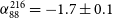 $\alpha_{88}^{216} = -1.7 \pm 0.1$
(Figure 26(viii)). As with Abell S1099, we consider this likely to be a remnant radio galaxy.
$\alpha_{88}^{216} = -1.7 \pm 0.1$
(Figure 26(viii)). As with Abell S1099, we consider this likely to be a remnant radio galaxy.
AqrCC 087. (i) Background: MWA-2, 216-MHz, robust
 $+0.5$
image. (ii) Background: RGB PS1 image (i, r, g). The white contours are as in Figure 2(i) for the background of (i) (with
$+0.5$
image. (ii) Background: RGB PS1 image (i, r, g). The white contours are as in Figure 2(i) for the background of (i) (with
 $\sigma_{\rm{rms}} = 1.1$
mJy beam−1). Red contours: NVSS image as in Figure 4(i). Cyan contours: RACS robust
$\sigma_{\rm{rms}} = 1.1$
mJy beam−1). Red contours: NVSS image as in Figure 4(i). Cyan contours: RACS robust
 $+0.25$
image, in levels of
$+0.25$
image, in levels of
 $[\pm 3, 6, 12, 24, 48] \times \sigma_{\rm{rms}}$
(
$[\pm 3, 6, 12, 24, 48] \times \sigma_{\rm{rms}}$
(
 $\sigma_{\rm{rms}} = 0.15$
mJy beam−1). Other image features are as in Figure 2, though note no scalebar is given as no redshift is available for the reported cluster.
$\sigma_{\rm{rms}} = 0.15$
mJy beam−1). Other image features are as in Figure 2, though note no scalebar is given as no redshift is available for the reported cluster.
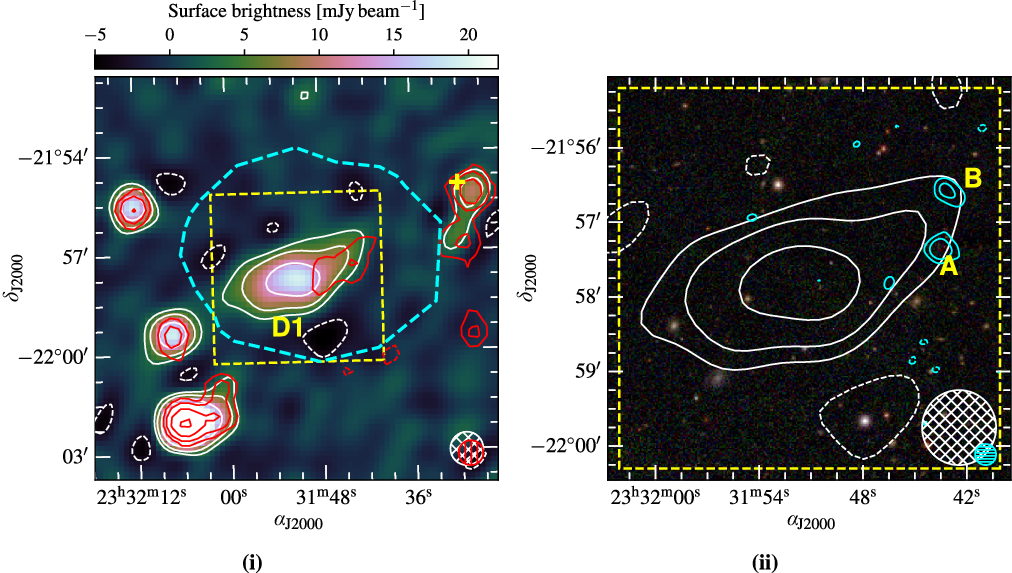
RXC J2351.0–1954 (PSZ1 G057.09-74.45) (Figure 10). Originally D21 reported three candidate sources: a halo at the centre (labelled D1 in Figure 10(i)), and two relics: SE (labelled D2, inset Figure 10(iii)), and NW, (labelled D3, inset Figure 10(ii)). The candidate halo is shown by the RACS data to be blended sources. The SE candidate relic detected at low significance (
 $\sim\!3\sigma$
), though the RACS data show a single compact source within the southern portion of the emission (Source A). The NW candidate relic is partially detected in RACS, with other compact blended sources (B–D in Figure 10(ii)). Excluding point sources, the LAS of D2 and D3 are 1.9 arcmin (
$\sim\!3\sigma$
), though the RACS data show a single compact source within the southern portion of the emission (Source A). The NW candidate relic is partially detected in RACS, with other compact blended sources (B–D in Figure 10(ii)). Excluding point sources, the LAS of D2 and D3 are 1.9 arcmin (
 ${\rm{LLS}}=230$
) and 3.5 arcmin (
${\rm{LLS}}=230$
) and 3.5 arcmin (
 ${\rm{LLS}}=430$
kpc), respectively. All labelled compact sources are subtracted from MWA measurements where appropriate. The spectral index of D2 is measured to be
${\rm{LLS}}=430$
kpc), respectively. All labelled compact sources are subtracted from MWA measurements where appropriate. The spectral index of D2 is measured to be
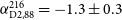 $\alpha_{{{\rm{D}}2},88}^{216} = -1.3 \pm 0.3$
(26(ix)). D3 shows significant curvature within the MWA band and to 887.5 MHz and is fit with a generic curved model, with a power law model fit across the MWA-2 band:
$\alpha_{{{\rm{D}}2},88}^{216} = -1.3 \pm 0.3$
(26(ix)). D3 shows significant curvature within the MWA band and to 887.5 MHz and is fit with a generic curved model, with a power law model fit across the MWA-2 band:
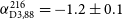 $\alpha_{{{\rm{D}}3},88}^{216} = -1.2 \pm 0.1$
(Figure 26(x)).The smoothed RASS image is shown as contours on Figure 10(i) showing elongation hinting at an un-relaxed ICM, though we consider that D3 is likely a remnant with the classical spectral steepening and D2 is still unconfirmed.
$\alpha_{{{\rm{D}}3},88}^{216} = -1.2 \pm 0.1$
(Figure 26(x)).The smoothed RASS image is shown as contours on Figure 10(i) showing elongation hinting at an un-relaxed ICM, though we consider that D3 is likely a remnant with the classical spectral steepening and D2 is still unconfirmed.
RXC J2351.0–1954. (i) Background: MWA-2, 154-MHz, robust
 $+0.5$
(ii) and (iii) Background: RGB PS1 image (i, r, g). The white contours are as in Figure 2(i) for the background of (i) (with
$+0.5$
(ii) and (iii) Background: RGB PS1 image (i, r, g). The white contours are as in Figure 2(i) for the background of (i) (with
 $\sigma_{\rm{rms}} = 4.9$
mJy beam−1). Red contours: TGSS image, in levels of
$\sigma_{\rm{rms}} = 4.9$
mJy beam−1). Red contours: TGSS image, in levels of
 $[\pm 3, 6, 12, 24, 48] \times \sigma_{\rm{rms}}$
(
$[\pm 3, 6, 12, 24, 48] \times \sigma_{\rm{rms}}$
(
 $\sigma_{\rm{rms}} = 3.6$
mJy beam−1). Cyan contours: RACS robust
$\sigma_{\rm{rms}} = 3.6$
mJy beam−1). Cyan contours: RACS robust
 $+0.25$
image, in levels of
$+0.25$
image, in levels of
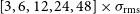 $[3, 6, 12, 24, 48] \times \sigma_{\rm{rms}}$
(
$[3, 6, 12, 24, 48] \times \sigma_{\rm{rms}}$
(
 $\sigma_{\rm{rms}} = 0.20$
mJy beam−1). Magenta contours: smoothed RASS image, increasing with factors of
$\sigma_{\rm{rms}} = 0.20$
mJy beam−1). Magenta contours: smoothed RASS image, increasing with factors of
 $\sqrt{2}$
. Other image features are as in Figure 2.
$\sqrt{2}$
. Other image features are as in Figure 2.
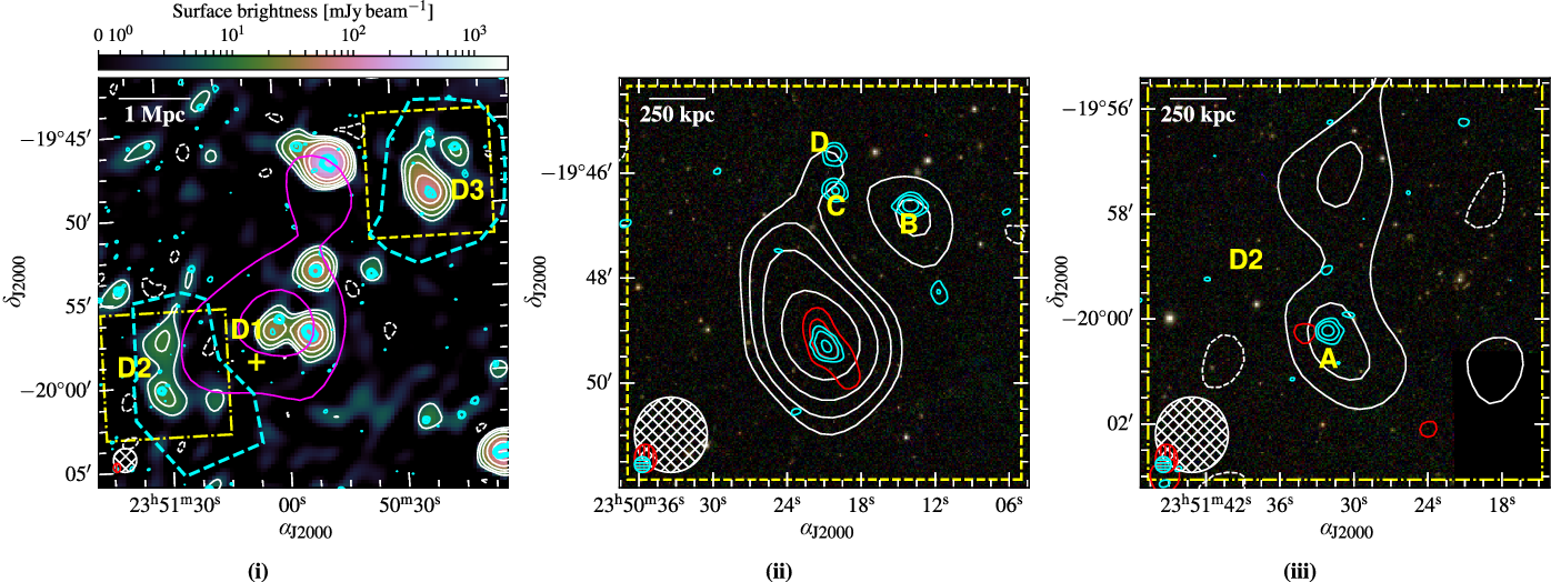
3.1.3. FIELD3
Abell 0168 Figure 11 shows the radio relic that was reported by Dwarakanath et al. (Reference Dwarakanath, Parekh, Kale and George2018) and is detected in the MWA-2 data. Dwarakanath et al. (Reference Dwarakanath, Parekh, Kale and George2018) split the total relic source into two distinct components–a large exterior component and a smaller interior component with a steeper spectrum. Here we consider it a single emission region due in part to the limitation of resolution but there also appears to be a fainter diffuse component connecting the two regions. While emission is detected in all MWA-2 bands (see e.g. 118-MHz in Figure 11), due to the large size (
 $\sim\!11.5$
arcmin) we note that flux recovery diminishes significantly in the 154-, 185-, and 216-MHz bands. With supplemental GLEAM data and flux densities reported by Dwarakanath et al. (Reference Dwarakanath, Parekh, Kale and George2018), we find the spectral index of the whole relic to be
$\sim\!11.5$
arcmin) we note that flux recovery diminishes significantly in the 154-, 185-, and 216-MHz bands. With supplemental GLEAM data and flux densities reported by Dwarakanath et al. (Reference Dwarakanath, Parekh, Kale and George2018), we find the spectral index of the whole relic to be
 $\alpha_{88}^{608} = -1.50 \pm 0.08$
.
$\alpha_{88}^{608} = -1.50 \pm 0.08$
.
Abell 0168. Background: MWA-2, 154-MHz, robust
 $+2.0$
image. The white contours are as in Figure 2(i) for the background image (with
$+2.0$
image. The white contours are as in Figure 2(i) for the background image (with
 $\sigma_{\rm{rms}} = 3.2$
mJy beam−1). Red contours: NVSS,
$\sigma_{\rm{rms}} = 3.2$
mJy beam−1). Red contours: NVSS,
 $[\pm 3, 6, 12, 24, 48] \times \sigma_{\rm{rms}}$
(
$[\pm 3, 6, 12, 24, 48] \times \sigma_{\rm{rms}}$
(
 $\sigma_{\rm{rms}} = 0.45$
mJy beam−1). Other image features are as in Figure 2, with a yellow circle with a 1 Mpc radius centred on the cluster.
$\sigma_{\rm{rms}} = 0.45$
mJy beam−1). Other image features are as in Figure 2, with a yellow circle with a 1 Mpc radius centred on the cluster.
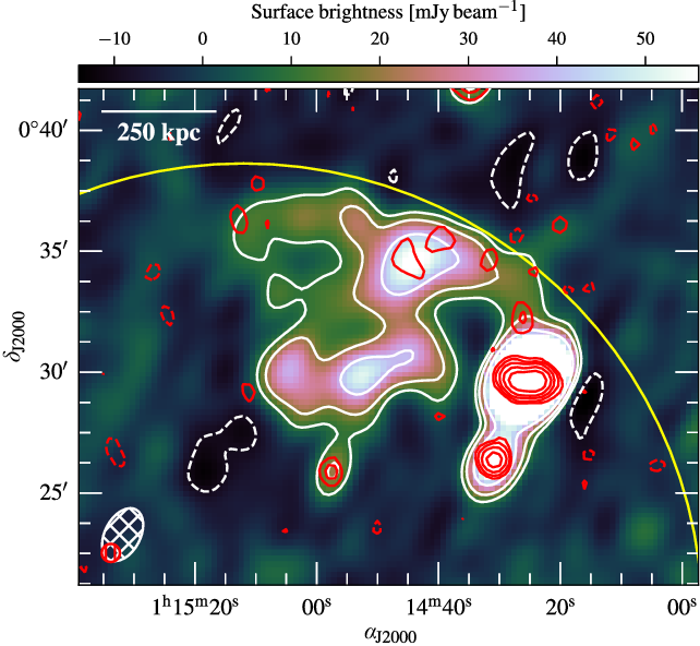
RXC J0137.2–0912 (Figure 12). We report the detection of steep-spectrum emission within RXC J0137.2–0912, shown in Figure 12(i) in MWA and TGSS data. 12(ii) shows the optical host of the central compact emission with contours from re-processed VAST data (cyan) overlaid. Figure 12(iii) shows the extent of the cluster’s X-ray emission with archival XMM-Newton data, noting some elongation perpendicular to the orientation of the radio emission. The compact emission from Sources A and B is subtracted after extrapolating to MWA-2 frequencies using the VAST and TGSS measurements, and C–E are subtracted assuming
 $\alpha = -0.7$
. A power law SED is modelled, with a spectral index of
$\alpha = -0.7$
. A power law SED is modelled, with a spectral index of
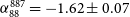 $\alpha_{88}^{887} = -1.62 \pm 0.07$
(Figure 26(xii), or
$\alpha_{88}^{887} = -1.62 \pm 0.07$
(Figure 26(xii), or
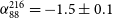 $\alpha_{88}^{216} = -1.5 \pm 0.1$
across the MWA band alone). The total angular size of the source is
$\alpha_{88}^{216} = -1.5 \pm 0.1$
across the MWA band alone). The total angular size of the source is
 $7.8$
arcmin, corresponding to 410 kpc. From the archival XMM-Newton data, we find a concentration parameter
$7.8$
arcmin, corresponding to 410 kpc. From the archival XMM-Newton data, we find a concentration parameter
 $c_{40/400} = 0.19$
, consistent with CC clusters (where non-CC clusters are found to have
$c_{40/400} = 0.19$
, consistent with CC clusters (where non-CC clusters are found to have
 $c_{40/400} \lesssim 0.075$
; Santos et al. Reference Santos, Rosati, Tozzi, Böhringer, Ettori and Bignamini2008). Based on the likelihood of a CC, the prominent BCG with significant AGN emission, and steep-spectrum diffuse emission surrounding the BCG we suggest the emission is a mini-halo. Some structure in the centre of the cluster gives some evidence for sloshing, and with a centroid shift within
$c_{40/400} \lesssim 0.075$
; Santos et al. Reference Santos, Rosati, Tozzi, Böhringer, Ettori and Bignamini2008). Based on the likelihood of a CC, the prominent BCG with significant AGN emission, and steep-spectrum diffuse emission surrounding the BCG we suggest the emission is a mini-halo. Some structure in the centre of the cluster gives some evidence for sloshing, and with a centroid shift within
 $R_{500} = 684$
kpc (Piffaretti et al. Reference Piffaretti, Arnaud, Pratt, Pointecouteau and Melin2011) of
$R_{500} = 684$
kpc (Piffaretti et al. Reference Piffaretti, Arnaud, Pratt, Pointecouteau and Melin2011) of
 $w = 0.037R_{500}$
suggesting some disturbance (Pratt et al. Reference Pratt, Croston, Arnaud and Böhringer2009; Böhringer et al. Reference Böhringer2010). While the orientation of the radio emission appears largely perpendicular to the X-ray emission, the extension to the SW in the radio is traced by an extension in the X-ray as well. The NE direction is ambiguous as the XMM-Newton exposure drops significantly due to a chip gap at that location. This is indicated on Figure 12(iii) as a dashed, magenta line.
$w = 0.037R_{500}$
suggesting some disturbance (Pratt et al. Reference Pratt, Croston, Arnaud and Böhringer2009; Böhringer et al. Reference Böhringer2010). While the orientation of the radio emission appears largely perpendicular to the X-ray emission, the extension to the SW in the radio is traced by an extension in the X-ray as well. The NE direction is ambiguous as the XMM-Newton exposure drops significantly due to a chip gap at that location. This is indicated on Figure 12(iii) as a dashed, magenta line.
RXC J0137.2–0912. (i) Background: MWA-2, 154-MHz, robust
 $0.0$
image. (ii) Background: RGB DES image (i, r, g). (ii) Background: smoothed XMM-Newton EPIC image. The white contours are as in Figure 2(i) for the background of (i) (with
$0.0$
image. (ii) Background: RGB DES image (i, r, g). (ii) Background: smoothed XMM-Newton EPIC image. The white contours are as in Figure 2(i) for the background of (i) (with
 $\sigma_{\rm{rms}} = 3.8$
mJy beam−1). Red contours: TGSS image, in levels of
$\sigma_{\rm{rms}} = 3.8$
mJy beam−1). Red contours: TGSS image, in levels of
 $[\pm 3, 6, 12, 24, 48] \times \sigma_{\rm{rms}}$
(
$[\pm 3, 6, 12, 24, 48] \times \sigma_{\rm{rms}}$
(
 $\sigma_{\rm{rms}} = 2.8$
mJy beam−1). Cyan contours: VAST
$\sigma_{\rm{rms}} = 2.8$
mJy beam−1). Cyan contours: VAST
 $+0.25$
image, in levels of
$+0.25$
image, in levels of
 $[\pm 3, 6, 12, 24, 48] \times \sigma_{\rm{rms}}$
(
$[\pm 3, 6, 12, 24, 48] \times \sigma_{\rm{rms}}$
(
 $\sigma_{\rm{rms}} = 0.14$
mJy beam−1). The dashed, magenta line on (iii) indicates the location of an XMM-Newton chip gap with lessened sensitivity. Other image features are as in Figure 2.
$\sigma_{\rm{rms}} = 0.14$
mJy beam−1). The dashed, magenta line on (iii) indicates the location of an XMM-Newton chip gap with lessened sensitivity. Other image features are as in Figure 2.
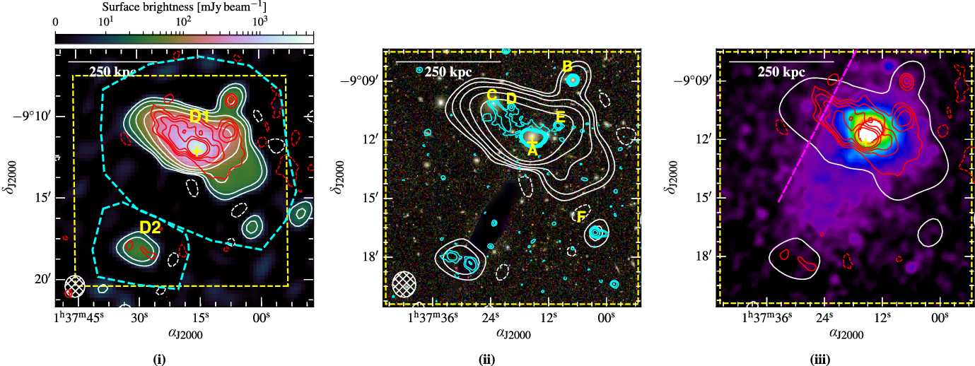
We see also an additional diffuse source resembling a remnant radio galaxy, D2; however, its SED shows significant curvature uncharacteristic of remnants (Figure 26(xiii)).
3.1.4. FIELD6
Abell S0112 (Figure 13). Abell S0112 is covered by the Australia Telescope Low Brightness Survey (ATLBS, region B; Subrahmanyan et al. Reference Subrahmanyan, Ekers, Saripalli and Sadler2010; Thorat et al. Reference Thorat, Subrahmanyan, Saripalli and Ekers2013) which reveals two extended radio galaxies (A and B) within the cluster. The MWA data reveal an additional emission component (D1) between the two bright radio galaxies, creating an asymmetric dumbbell shape. The emission is only detected across the MWA-2 band, from 88–185 MHz and in the 200-MHz GLEAM data. The extent of the emission between the two radio galaxies is
 $\sim\!3$
arcmin (
$\sim\!3$
arcmin (
 ${\rm{LLS}}\approx 230$
kpc). We measure integrated flux density within the D1 region between A and B, finding a spectral index of
${\rm{LLS}}\approx 230$
kpc). We measure integrated flux density within the D1 region between A and B, finding a spectral index of
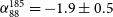 $\alpha_{88}^{185} = -1.9 \pm 0.5$
Figure 26(xiv)). In Figure 13(ii) we show optical data which reveals a lack of obvious optical host for the emission, and Figure 13(iii) shows the XMM-Newton image, highlighting the offset of the emission from the main component of the X-ray–emitting ICM. Source A is an active radio galaxy with a normal a radio spectrum (
$\alpha_{88}^{185} = -1.9 \pm 0.5$
Figure 26(xiv)). In Figure 13(ii) we show optical data which reveals a lack of obvious optical host for the emission, and Figure 13(iii) shows the XMM-Newton image, highlighting the offset of the emission from the main component of the X-ray–emitting ICM. Source A is an active radio galaxy with a normal a radio spectrum (
 $\alpha \sim -0.8$
), and D1 may be associated with an older episode of outflow. This could be true for B as well, with the extension of B to the north in the MWA-2 data also suggesting additional emission components not detected in higher-frequency/resolution images. We consider this emission fossil plasma associated with either A or B, with potential for some re-acceleration due to the dynamic nature of the cluster.
$\alpha \sim -0.8$
), and D1 may be associated with an older episode of outflow. This could be true for B as well, with the extension of B to the north in the MWA-2 data also suggesting additional emission components not detected in higher-frequency/resolution images. We consider this emission fossil plasma associated with either A or B, with potential for some re-acceleration due to the dynamic nature of the cluster.
Abell S0112. (i) Background: MWA-2, 154-MHz, robust
 $+2.0$
image. (ii) Background: RGB SSS image (i, r, b). (iii). Background: smoothed XMM-Newton EPIC image. The white contours are as in Figure 2(i) for the background of (i) (with
$+2.0$
image. (ii) Background: RGB SSS image (i, r, b). (iii). Background: smoothed XMM-Newton EPIC image. The white contours are as in Figure 2(i) for the background of (i) (with
 $\sigma_{\rm{rms}} = 3.5$
mJy beam−1). Magenta contours: ATLBS high-resolution image, in levels of
$\sigma_{\rm{rms}} = 3.5$
mJy beam−1). Magenta contours: ATLBS high-resolution image, in levels of
 $[\pm 3, 6, 12, 24, 48] \times \sigma_{\rm{rms}}$
(
$[\pm 3, 6, 12, 24, 48] \times \sigma_{\rm{rms}}$
(
 $\sigma_{\rm{rms}} = 0.08$
mJy beam−1). Cyan contours: RACS survey image, in levels of
$\sigma_{\rm{rms}} = 0.08$
mJy beam−1). Cyan contours: RACS survey image, in levels of
 $[\pm 3, 6, 12, 24, 48] \times \sigma_{\rm{rms}}$
(
$[\pm 3, 6, 12, 24, 48] \times \sigma_{\rm{rms}}$
(
 $\sigma_{\rm{rms}} = 0.29$
mJy beam−1). Other image features are as in Figure 2.
$\sigma_{\rm{rms}} = 0.29$
mJy beam−1). Other image features are as in Figure 2.
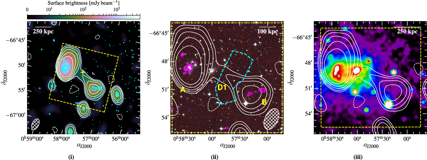
MCXC J0145.2–6033 (Figure 14). We report the detection of a candidate mini-halo in MWA-2 and RACS data, shown in Figure 14(i). The detection is marginal in the RACS data, and
 $2\sigma$
contours of the low resolution image are shown in Figure 14(i) to highlight the extent of the emission. Figure 14(i) shows the robust
$2\sigma$
contours of the low resolution image are shown in Figure 14(i) to highlight the extent of the emission. Figure 14(i) shows the robust
 $+0.25$
RACS data which stems from the BCG and extends northwards. We measure the flux densities across the available images and find
$+0.25$
RACS data which stems from the BCG and extends northwards. We measure the flux densities across the available images and find
 $\alpha_{88}^{887} = -2.1 \pm 0.1$
(Figure 26(xv), with the same value across only the MWA-2 band). The extent of the source is
$\alpha_{88}^{887} = -2.1 \pm 0.1$
(Figure 26(xv), with the same value across only the MWA-2 band). The extent of the source is
 ${{\rm{LAS}}} = 1.9$
arcmin;
${{\rm{LAS}}} = 1.9$
arcmin;
 ${{\rm{LLS}}} = 350$
kpc. The optical data is shown in Figure 14(ii), with a BCG clear near the centre of the emission. RASS data shown in Figure 14(iii) does not show any significant offset from the BCG, and we suggest the cluster is reasonably relaxed. With an LAS of 1.9 arcmin (
${{\rm{LLS}}} = 350$
kpc. The optical data is shown in Figure 14(ii), with a BCG clear near the centre of the emission. RASS data shown in Figure 14(iii) does not show any significant offset from the BCG, and we suggest the cluster is reasonably relaxed. With an LAS of 1.9 arcmin (
 ${\rm{LLS}}=350$
kpc), the source is only barely extended in the robust
${\rm{LLS}}=350$
kpc), the source is only barely extended in the robust
 $+2.0$
MWA-2 images, and the robust
$+2.0$
MWA-2 images, and the robust
 $0.0$
images show no significant extension. There is a
$0.0$
images show no significant extension. There is a
 $\sim\!20$
mJy difference between the 0.0 and
$\sim\!20$
mJy difference between the 0.0 and
 $+2.0$
measurements at 154 MHz (
$+2.0$
measurements at 154 MHz (
 $S_{{r0}} = 110 \pm 10$
and
$S_{{r0}} = 110 \pm 10$
and
 $S_{r2} = 130 \pm 10$
) which may be allowable within uncertainties. Given the low SNR in the RACS data, it is difficult to confirm if this is an ultra-steep spectrum point source.
$S_{r2} = 130 \pm 10$
) which may be allowable within uncertainties. Given the low SNR in the RACS data, it is difficult to confirm if this is an ultra-steep spectrum point source.
MCXC J0145.2–6033. (i) Background: MWA-2, 154-MHz, robust
 $+2.0$
image. (ii) Background: RGB DES image (i, r, g). (iii) Background: smoothed RASS image. The white (black) contours are as in Figure 2(i) for the background of (i) (with
$+2.0$
image. (ii) Background: RGB DES image (i, r, g). (iii) Background: smoothed RASS image. The white (black) contours are as in Figure 2(i) for the background of (i) (with
 $\sigma_{\rm{rms}} = 2.9$
mJy beam−1). Red contours: RACS low-resolution image,
$\sigma_{\rm{rms}} = 2.9$
mJy beam−1). Red contours: RACS low-resolution image,
 $[\pm 3, 6, 12, 24, 48] \times \sigma_{\rm{rms}}$
(
$[\pm 3, 6, 12, 24, 48] \times \sigma_{\rm{rms}}$
(
 $\sigma_{\rm{rms}} = 0.34$
mJy beam-1). Cyan contours: RACS robust
$\sigma_{\rm{rms}} = 0.34$
mJy beam-1). Cyan contours: RACS robust
 $+0.25$
image,
$+0.25$
image,
 $[\pm 3, 6, 12, 24, 48] \times \sigma_{\rm{rms}}$
(
$[\pm 3, 6, 12, 24, 48] \times \sigma_{\rm{rms}}$
(
 $\sigma_{\rm{rms}} = 0.17$
mJy beam−1). Magenta contours: MWA-2, 216-MHz, robust
$\sigma_{\rm{rms}} = 0.17$
mJy beam−1). Magenta contours: MWA-2, 216-MHz, robust
 $0.0$
image,
$0.0$
image,
 $[\pm 3, 6, 12, 24, 48] \times \sigma_{\rm{rms}}$
(
$[\pm 3, 6, 12, 24, 48] \times \sigma_{\rm{rms}}$
(
 $\sigma_{\rm{rms}} = 3.4$
mJy beam−1). Other image features are as in Figure 2.
$\sigma_{\rm{rms}} = 3.4$
mJy beam−1). Other image features are as in Figure 2.
MCXC J0154.2–5937 (Figure 15). We report peripherally located, elongated extended emission in the cluster, shown in Figure 15(i). In Figure 15(ii) a potential optical host is seen with matching emission in the RACS image (Source A,
 $S_{887} \sim 1$
mJy, WISEA J015436.21–593929.9, no redshift). The radio SED of the whole source is uncertain, but consistent with a radio galaxy (
$S_{887} \sim 1$
mJy, WISEA J015436.21–593929.9, no redshift). The radio SED of the whole source is uncertain, but consistent with a radio galaxy (
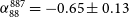 $\alpha_{88}^{887} = -0.65 \pm 0.13$
; Figure 26(xvi)). If in the cluster, the source is
$\alpha_{88}^{887} = -0.65 \pm 0.13$
; Figure 26(xvi)). If in the cluster, the source is
 $\sim\!1$
Mpc in projected extent, classing it as a giant radio galaxy.
$\sim\!1$
Mpc in projected extent, classing it as a giant radio galaxy.
MCXC J0154.2–5937. (i) Background: MWA-2, 154-MHz, robust
 $+2.0$
image. (ii) Background: RGB DES image (i, r, g). (iii) Background: smoothed XMM-Newton EPIC image. The white contours are as in Figure 2(i) for the background of (i) (with
$+2.0$
image. (ii) Background: RGB DES image (i, r, g). (iii) Background: smoothed XMM-Newton EPIC image. The white contours are as in Figure 2(i) for the background of (i) (with
 $\sigma_{\rm{rms}} = 2.5$
mJy beam−1). Red contours: RACS low-resolution image,
$\sigma_{\rm{rms}} = 2.5$
mJy beam−1). Red contours: RACS low-resolution image,
 $[\pm 3, 6, 12, 24, 48] \times \sigma_{\rm{rms}}$
(
$[\pm 3, 6, 12, 24, 48] \times \sigma_{\rm{rms}}$
(
 $\sigma_{\rm{rms}} = 0.40$
mJy beam−1). Cyan contours: RACS robust
$\sigma_{\rm{rms}} = 0.40$
mJy beam−1). Cyan contours: RACS robust
 $+0.0$
image,
$+0.0$
image,
 $[\pm 3, 6, 12, 24, 48] \times \sigma_{\rm{rms}}$
(
$[\pm 3, 6, 12, 24, 48] \times \sigma_{\rm{rms}}$
(
 $\sigma_{\rm{rms}} = 0.20$
mJy beam−1). Other image features are as in Figure 2.
$\sigma_{\rm{rms}} = 0.20$
mJy beam−1). Other image features are as in Figure 2.
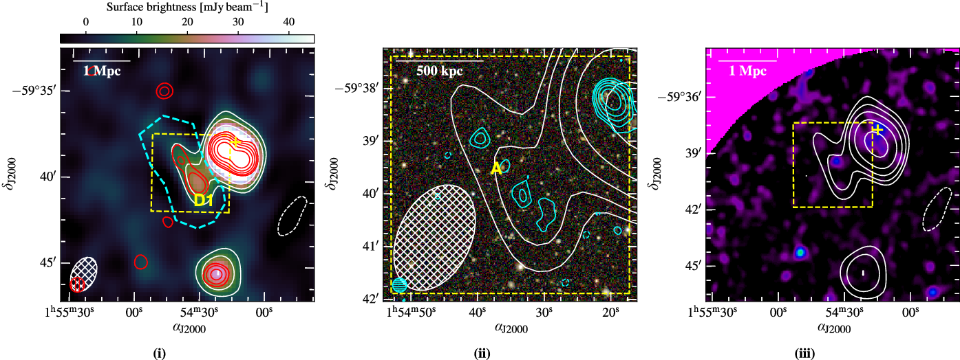
3.1.5. FIELD7
Abell 3186 (Figure 16). From the data presented here we report Abell 3186 to be a double relic system, potentially with central diffuse emission possible from a radio halo. The cluster shows a similar morphology to older observations of the canonical double relic cluster Abell 3667 (Johnston-Hollitt Reference Johnston-Hollitt2003; Hindson et al. Reference Hindson2014) with a larger, bright relic on one side and a smaller dimmer one on the other.
Abell 3186. (i) Background: MWA-2, 88-MHz, robust
 $+2.0$
image. (iii) and (iv) Background: RGB SSS image (i, r, b). (ii) Background: smoothed XMM-Newton EPIC image. The white contours are as in Figure 2(i) for the background of (i) (with
$+2.0$
image. (iii) and (iv) Background: RGB SSS image (i, r, b). (ii) Background: smoothed XMM-Newton EPIC image. The white contours are as in Figure 2(i) for the background of (i) (with
 $\sigma_{\rm{rms}} = 15$
mJy beam−1). Red contours: deep ASKAP low-resolution image,
$\sigma_{\rm{rms}} = 15$
mJy beam−1). Red contours: deep ASKAP low-resolution image,
 $[\pm 3, 6, 12, 24, 48] \times \sigma_{\rm{rms}}$
(
$[\pm 3, 6, 12, 24, 48] \times \sigma_{\rm{rms}}$
(
 $\sigma_{\rm{rms}} = 0.70$
mJy beam−1). Cyan contours: deep ASKAP robust
$\sigma_{\rm{rms}} = 0.70$
mJy beam−1). Cyan contours: deep ASKAP robust
 $+0.25$
,
$+0.25$
,
 $[\pm 3, 6, 12, 24, 48] \times \sigma_{\rm{rms}}$
(
$[\pm 3, 6, 12, 24, 48] \times \sigma_{\rm{rms}}$
(
 $\sigma_{\rm{rms}} = 0.32$
mJy beam−1 and
$\sigma_{\rm{rms}} = 0.32$
mJy beam−1 and
 $\sigma_{\rm{rms}} = 0.25$
mJy beam−1 for (iii) and (iv), respectively). Other image features are as in Figures 2 and 3, with the magenta box indicating the location of (iv) on (i) and (ii).
$\sigma_{\rm{rms}} = 0.25$
mJy beam−1 for (iii) and (iv), respectively). Other image features are as in Figures 2 and 3, with the magenta box indicating the location of (iv) on (i) and (ii).
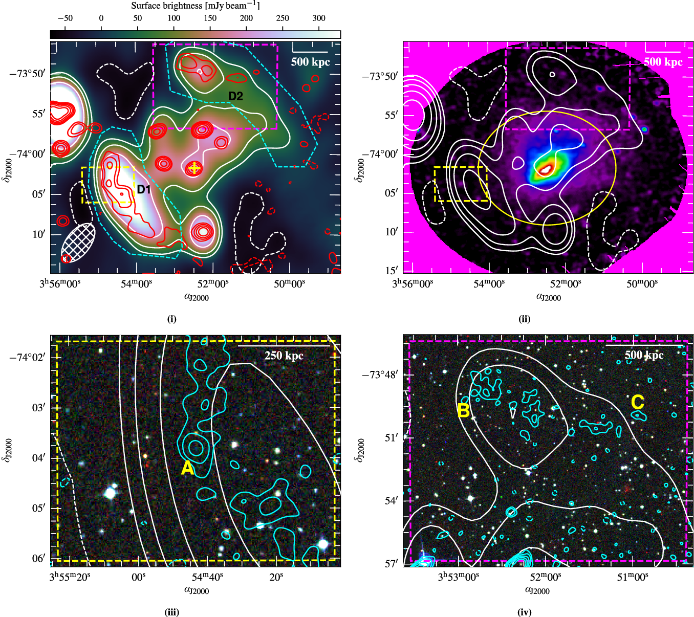
The larger relic, D1, is detected to the SW as an elongated structure on the periphery of Abell 3186 with the MWA and ASKAP, shown in Figure 16(i). The angular extent of D1 is
 $\sim\!12$
arcmin, corresponding to
$\sim\!12$
arcmin, corresponding to
 $\sim\!1650$
kpc. The MWA-2 images in this region at 154-, 185-, and 216-MHz, which are generally less sensitive, suffered from significant noise from a nearby bright source and the large relic is poorly detected. A somewhat compact source is detected within the emission (Source A) which has a faint, blue optical counterpart, seen in Figure 16(iii). After subtracting the contribution from A, we obtain a spectral index of
$\sim\!1650$
kpc. The MWA-2 images in this region at 154-, 185-, and 216-MHz, which are generally less sensitive, suffered from significant noise from a nearby bright source and the large relic is poorly detected. A somewhat compact source is detected within the emission (Source A) which has a faint, blue optical counterpart, seen in Figure 16(iii). After subtracting the contribution from A, we obtain a spectral index of
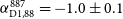 $\alpha_{{D1},88}^{887} = -1.0 \pm 0.1$
(Figure 16(xvii)), consistent with relic sources. We show the XMM-Newton image in Figure 16(ii), and note that Lovisari et al. (Reference Lovisari2017) report the cluster has a ‘mixed’ morphology (i.e. semi-disturbed). Additionally, the cluster hosts a second relic to the NW seen as a patchy structure, with detections in all bands, though the full extent of the emission (
$\alpha_{{D1},88}^{887} = -1.0 \pm 0.1$
(Figure 16(xvii)), consistent with relic sources. We show the XMM-Newton image in Figure 16(ii), and note that Lovisari et al. (Reference Lovisari2017) report the cluster has a ‘mixed’ morphology (i.e. semi-disturbed). Additionally, the cluster hosts a second relic to the NW seen as a patchy structure, with detections in all bands, though the full extent of the emission (
 $\sim\!14$
arcmin,
$\sim\!14$
arcmin,
 $\sim\!1900$
kpc), extending to the SW, is only seen at 88 and 118 MHz as with D1. After subtraction of discrete source contributions (labelled B and C in Figure 16(iv)), we derive a spectral index of
$\sim\!1900$
kpc), extending to the SW, is only seen at 88 and 118 MHz as with D1. After subtraction of discrete source contributions (labelled B and C in Figure 16(iv)), we derive a spectral index of
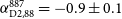 $\alpha_{{{\rm{D}}2},88}^{887} = -0.9 \pm 0.1$
. The morphology and spectral properties of these relics are extremely reminiscent of Abell 3667 which as a bright, larger relic and a smaller more compact relic with average spectral indices of
$\alpha_{{{\rm{D}}2},88}^{887} = -0.9 \pm 0.1$
. The morphology and spectral properties of these relics are extremely reminiscent of Abell 3667 which as a bright, larger relic and a smaller more compact relic with average spectral indices of
 $-0.9$
for both across MWA bands (Hindson et al. Reference Hindson2014), though higher resolution, higher frequency spectral index measurements show
$-0.9$
for both across MWA bands (Hindson et al. Reference Hindson2014), though higher resolution, higher frequency spectral index measurements show
 $\alpha$
varies inside the relics from approximately
$\alpha$
varies inside the relics from approximately
 $-0.8$
to
$-0.8$
to
 $-1$
(Johnston-Hollitt Reference Johnston-Hollitt2003). We consider this a classical double relic system. We note also the 88-MHz MWA-2 image (Figure 16(i)) appears to show an excess of diffuse flux within the central cluster region which may indicate a radio halo, though the confusion from sources in the cluster make this impossible to confirm with the present data.
$-1$
(Johnston-Hollitt Reference Johnston-Hollitt2003). We consider this a classical double relic system. We note also the 88-MHz MWA-2 image (Figure 16(i)) appears to show an excess of diffuse flux within the central cluster region which may indicate a radio halo, though the confusion from sources in the cluster make this impossible to confirm with the present data.
Abell S0405 (Figure 17). We report a diffuse source in Abell S0405, with RACS data revealing a double-lobed radio galaxy structure (Figure 17(i)) without a core or jets. No obvious optical host exists between the two lobes (Figure 17(ii)) and we suggest this is a remnant radio galaxy. We find
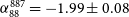 $\alpha_{88}^{887} = -1.99 \pm 0.08$
between the MWA and RACS data, after subtraction of Sources A and B from the MWA images (Figure 26(xix)). The source is measured to be
$\alpha_{88}^{887} = -1.99 \pm 0.08$
between the MWA and RACS data, after subtraction of Sources A and B from the MWA images (Figure 26(xix)). The source is measured to be
 $\sim\!185$
kpc if at the redshift of the cluster (
$\sim\!185$
kpc if at the redshift of the cluster (
 $z=0.0613$
; De Grandi et al. Reference De Grandi1999), and sits within the X-ray–emitting ICM (Figure 17(iii)).
$z=0.0613$
; De Grandi et al. Reference De Grandi1999), and sits within the X-ray–emitting ICM (Figure 17(iii)).
Abell S0405. (i) Background: MWA-2, 154-MHz, robust
 $+2.0$
image. (ii) Background: RGB SSS image (i, r, b). (iii). Background: smoothed Chandra image. The white contours are as in Figure 2(i) for the background of (i) (with
$+2.0$
image. (ii) Background: RGB SSS image (i, r, b). (iii). Background: smoothed Chandra image. The white contours are as in Figure 2(i) for the background of (i) (with
 $\sigma_{\rm{rms}} = 10$
mJy beam−1). Cyan contours: RACS survey image,
$\sigma_{\rm{rms}} = 10$
mJy beam−1). Cyan contours: RACS survey image,
 $[\pm 3, 6, 12, 24, 48] \times \sigma_{\rm{rms}}$
(
$[\pm 3, 6, 12, 24, 48] \times \sigma_{\rm{rms}}$
(
 $\sigma_{\rm{rms}} = 0.28$
mJy beam−1). Other image features are as in Figure 2.
$\sigma_{\rm{rms}} = 0.28$
mJy beam−1). Other image features are as in Figure 2.
PSZ1 G287.95–32.98
Footnote
w
(Figure 18). We report the detection of a diffuse source at the cluster centre with the MWA at 118 and 154 MHz as well as a partial detection at 887 MHz in RACS data. The projected size of the source is
 $\sim\!320$
kpc. Other MWA bands either suffer from lack of sensitivity or significant confusion with nearby Sources A and B (Figure 18(i)). We obtain a spectral index of
$\sim\!320$
kpc. Other MWA bands either suffer from lack of sensitivity or significant confusion with nearby Sources A and B (Figure 18(i)). We obtain a spectral index of
 $\alpha_{118}^{887} =-1.5 \pm 0.2$
(Figure 26(xx)). Figure 18(iii) shows the XMM-Newton image, highlighting the central location of the candidate radio halo. Based on the XMM-Newton data, Rossetti et al. (Reference Rossetti, Gastaldello, Eckert, Della Torre, Pantiri, Cazzoletti and Molendi2017) use the concentration parameter (see Santos et al. Reference Santos, Rosati, Tozzi, Böhringer, Ettori and Bignamini2008) to determine the cluster is a non-CC cluster, and the emission is therefore unlikely to be a mini-halo. Additionally, no obvious BCG with core radio emission is seen in the optical data shown in Figure 18(ii). We classify this source as a candidate radio halo.
$\alpha_{118}^{887} =-1.5 \pm 0.2$
(Figure 26(xx)). Figure 18(iii) shows the XMM-Newton image, highlighting the central location of the candidate radio halo. Based on the XMM-Newton data, Rossetti et al. (Reference Rossetti, Gastaldello, Eckert, Della Torre, Pantiri, Cazzoletti and Molendi2017) use the concentration parameter (see Santos et al. Reference Santos, Rosati, Tozzi, Böhringer, Ettori and Bignamini2008) to determine the cluster is a non-CC cluster, and the emission is therefore unlikely to be a mini-halo. Additionally, no obvious BCG with core radio emission is seen in the optical data shown in Figure 18(ii). We classify this source as a candidate radio halo.
PSZ1 G287.95–32.98. (i) Background: MWA-2, 154-MHz, robust
 $+2.0$
image. (ii) Background: RGB SSS image (i, r, b). (iii). Background: smoothed XMM-Newton image. The white contours are as in Figure 2(i) for the background of (i) (with
$+2.0$
image. (ii) Background: RGB SSS image (i, r, b). (iii). Background: smoothed XMM-Newton image. The white contours are as in Figure 2(i) for the background of (i) (with
 $\sigma_{\rm{rms}} = 6.6$
mJy beam−1). Red contours: RACS low resolution image
$\sigma_{\rm{rms}} = 6.6$
mJy beam−1). Red contours: RACS low resolution image
 $[\pm 3, 6, 12, 24, 48] \times \sigma_{\rm{rms}}$
(
$[\pm 3, 6, 12, 24, 48] \times \sigma_{\rm{rms}}$
(
 $\sigma_{\rm{rms}} = 0.25$
mJy beam−1). Cyan contours: RACS robust
$\sigma_{\rm{rms}} = 0.25$
mJy beam−1). Cyan contours: RACS robust
 $+0.25$
image,
$+0.25$
image,
 $[\pm 3, 6, 12, 24, 48] \times \sigma_{\rm{rms}}$
(
$[\pm 3, 6, 12, 24, 48] \times \sigma_{\rm{rms}}$
(
 $\sigma_{\rm{rms}} = 0.15$
mJy beam-1). Other image features are as in Figure 2.
$\sigma_{\rm{rms}} = 0.15$
mJy beam-1). Other image features are as in Figure 2.
3.1.6. FIELD8
Abell 3399 (Figure 19). We report the detection of a candidate radio relic on the periphery of Abell 3399 (D1 in Figure 19(i)) with an angular extent of
 $\sim\!3.6$
arcmin (
$\sim\!3.6$
arcmin (
 ${\rm{LLS}}\approx 710$
kpc) and a candidate radio halo at the centre of the cluster (D2 in Figure 19(i)) with an angular extent of
${\rm{LLS}}\approx 710$
kpc) and a candidate radio halo at the centre of the cluster (D2 in Figure 19(i)) with an angular extent of
 $\sim\!2.8$
arcmin (
$\sim\!2.8$
arcmin (
 ${\rm{LLS}}\approx 570$
kpc). As is clear from the Chandra X-ray data shown in Figure 19(ii), the cluster is undergoing a merger and Lovisari et al. (Reference Lovisari2017) consider the cluster ‘disturbed’ based on morphological analysis. Measuring flux densities of D1 at 88–154, and 887.5 MHz yields a spectral index of
${\rm{LLS}}\approx 570$
kpc). As is clear from the Chandra X-ray data shown in Figure 19(ii), the cluster is undergoing a merger and Lovisari et al. (Reference Lovisari2017) consider the cluster ‘disturbed’ based on morphological analysis. Measuring flux densities of D1 at 88–154, and 887.5 MHz yields a spectral index of
 $\alpha _{{\rm{D}}1,88}^{887} = - 1.6 \pm 0.3$
(Figure 26(xxi)). For D2, the emission is is barely detected between 154–216 MHz and the 88-MHz image is too confused with D1 for a useful measurement. We instead calculate the two-point spectral index between 118 and 887 MHz, finding
$\alpha _{{\rm{D}}1,88}^{887} = - 1.6 \pm 0.3$
(Figure 26(xxi)). For D2, the emission is is barely detected between 154–216 MHz and the 88-MHz image is too confused with D1 for a useful measurement. We instead calculate the two-point spectral index between 118 and 887 MHz, finding
 $\alpha _{{\rm{D}}2,118}^{887} = - 1.5 \pm 0.2$
(Figure 26(xxii), though note the line shown is derived from the two-point index and not a fitted power law model).
$\alpha _{{\rm{D}}2,118}^{887} = - 1.5 \pm 0.2$
(Figure 26(xxii), though note the line shown is derived from the two-point index and not a fitted power law model).
Abell 3399. (i) Background: MWA-2, 118-MHz, robust
 $+2.0$
image. (ii) Background: RGB SSS image (i, r, b). (iii) Background: smoothed Chandra image. The white contours are as in Figure 2(i) for the background of (i) (with
$+2.0$
image. (ii) Background: RGB SSS image (i, r, b). (iii) Background: smoothed Chandra image. The white contours are as in Figure 2(i) for the background of (i) (with
 $\sigma_{\rm{rms}} = 7.3$
mJy beam−1). Red contours: RACS discrete source-subtracted image,
$\sigma_{\rm{rms}} = 7.3$
mJy beam−1). Red contours: RACS discrete source-subtracted image,
 $[\pm 3, 6, 12, 24, 48] \times \sigma_{\rm{rms}}$
(
$[\pm 3, 6, 12, 24, 48] \times \sigma_{\rm{rms}}$
(
 $\sigma_{\rm{rms}} = 0.45$
mJy beam−1). Cyan contours: RACS survey image,
$\sigma_{\rm{rms}} = 0.45$
mJy beam−1). Cyan contours: RACS survey image,
 $[\pm 3, 6, 12, 24, 48] \times \sigma_{\rm{rms}}$
(
$[\pm 3, 6, 12, 24, 48] \times \sigma_{\rm{rms}}$
(
 $\sigma_{\rm{rms}} = 0.17$
mJy beam−1). Other image features are as in Figure 2.
$\sigma_{\rm{rms}} = 0.17$
mJy beam−1). Other image features are as in Figure 2.
3.1.7. FIELD9
MCXC J1253.2–1522 (Abell 1631) (Figure 20). We report a steep spectrum source projected onto MCXC J1253.2–1522 in MWA data, with no counterpart in RACS, and marginal detection in the TGSS image (Figure 20(i)). Note the TGSS image has artefacts from the nearby complex radio galaxy that peak at the location of the diffuse source. Multiple cluster systems are reported along line of sight: MCXC J1253.2–1522 at
 $z=0.0462$
(Piffaretti et al. Reference Piffaretti, Arnaud, Pratt, Pointecouteau and Melin2011) and Abell 1631 at
$z=0.0462$
(Piffaretti et al. Reference Piffaretti, Arnaud, Pratt, Pointecouteau and Melin2011) and Abell 1631 at
 $z=0.01394$
(Coziol et al. Reference Coziol, Andernach, Caretta, Alamo-MartÍnez and Tago2009). Additionally, Flin & Krywult (Reference Flin and Krywult2006) report that the system has complex substructure, which is clear in the smoothed RASS image shown in Figure 20(iii). No obvious optical host is visible in PS1 data (Figure 20(i), and the projected linear extent is 200 kpc (or 70 kpc if at
$z=0.01394$
(Coziol et al. Reference Coziol, Andernach, Caretta, Alamo-MartÍnez and Tago2009). Additionally, Flin & Krywult (Reference Flin and Krywult2006) report that the system has complex substructure, which is clear in the smoothed RASS image shown in Figure 20(iii). No obvious optical host is visible in PS1 data (Figure 20(i), and the projected linear extent is 200 kpc (or 70 kpc if at
 $z=0.01394$
). While just outside of the field of view (FoV) of archival XMM-Newton observations, RASS shows no significant X-ray emission at the location of the source, but the source sits between two X-ray clumps. We find the spectral index to be
$z=0.01394$
). While just outside of the field of view (FoV) of archival XMM-Newton observations, RASS shows no significant X-ray emission at the location of the source, but the source sits between two X-ray clumps. We find the spectral index to be
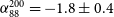 $\alpha_{88}^{200} = -1.8 \pm 0.4$
(Figure 26(xxiii)), and suggest the source is fossil plasma or otherwise a remnant radio galaxy.
$\alpha_{88}^{200} = -1.8 \pm 0.4$
(Figure 26(xxiii)), and suggest the source is fossil plasma or otherwise a remnant radio galaxy.
MCXC J1253.2–1522 (Abell 1631). (i) Background: MWA-2, 118-MHz, robust
 $+2.0$
image. (ii) Background: RGB PS1 image (i, r, g). (iii) Background: smoothed RASS image. The white (black) contours are as in Figure 2(i) for the background of (i) (with
$+2.0$
image. (ii) Background: RGB PS1 image (i, r, g). (iii) Background: smoothed RASS image. The white (black) contours are as in Figure 2(i) for the background of (i) (with
 $\sigma_{\rm{rms}} = 7.0$
mJy beam−1). Red contours: TGSS image,
$\sigma_{\rm{rms}} = 7.0$
mJy beam−1). Red contours: TGSS image,
 $[\pm 3, 6, 12, 24, 48] \times \sigma_{\rm{rms}}$
(
$[\pm 3, 6, 12, 24, 48] \times \sigma_{\rm{rms}}$
(
 $\sigma_{\rm{rms}} = 3.5$
mJy beam−1). Cyan contours: RACS survey image,
$\sigma_{\rm{rms}} = 3.5$
mJy beam−1). Cyan contours: RACS survey image,
 $[3, 6, 12, 24, 48] \times \sigma_{\rm{rms}}$
(
$[3, 6, 12, 24, 48] \times \sigma_{\rm{rms}}$
(
 $\sigma_{\rm{rms}} = 0.32$
mJy beam−1). Other image features are as in Figure 2, with the addition of a separate, yellow linear scale at the redshift of Abell 1631.
$\sigma_{\rm{rms}} = 0.32$
mJy beam−1). Other image features are as in Figure 2, with the addition of a separate, yellow linear scale at the redshift of Abell 1631.
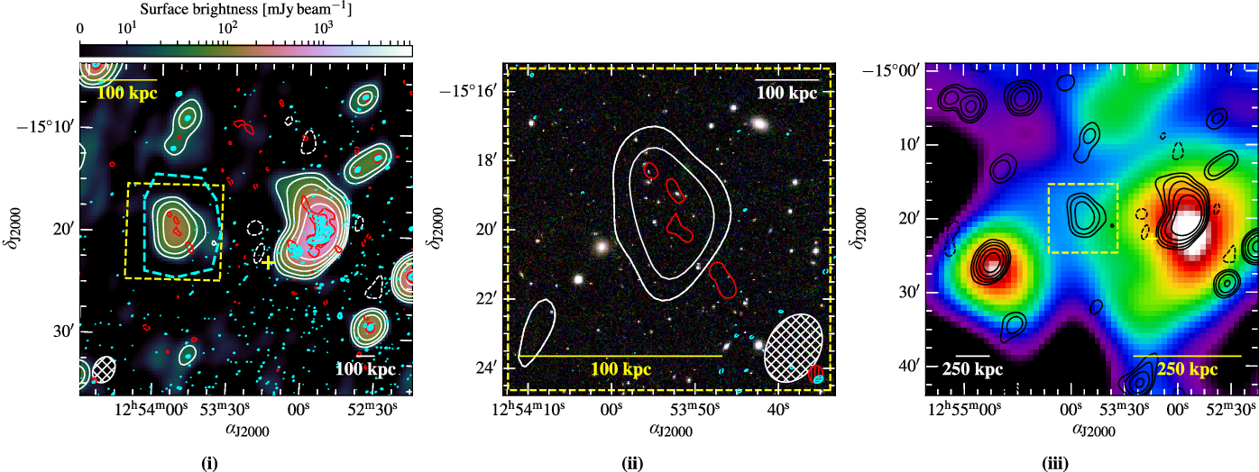
3.1.8. FIELD10
Abell 3164 (Figure 21). MWA and the VAST data reveal a complex radio galaxy with at least three distinct remnant components (D1–3 in Figure 21(i)) with LASs 3.5, 3.8, and 3.1 arcmin and LLSs of 240, 260, and 210 kpc for D1–3, respectively. The head-tail (HT) galaxy (hosted by FAIRALL 0757; Fairall Reference Fairall1984) in the cluster is clearly connected to D3 and is likely responsible for at least D2, however, it is not clear whether D1 has spawned from the same galaxy. The source-subtracted VAST data is shown in Figure 21(i) and highlights the steepness of D2. After subtraction of Sources A and B from the relevant measurements, we obtain spectral indices of D1:
 $\alpha_{88}^{887} = -1.48 \pm 0.08$
(Figure 26(xxiv)), D2:
$\alpha_{88}^{887} = -1.48 \pm 0.08$
(Figure 26(xxiv)), D2:
 $\alpha_{88}^{216} = -2.3 \pm 0.1$
(though Figure 26(xxiv) shows some curvature within the MWA band, and D2 is also fit with a generic curved model between 88–887.5 MHz), D3:
$\alpha_{88}^{216} = -2.3 \pm 0.1$
(though Figure 26(xxiv) shows some curvature within the MWA band, and D2 is also fit with a generic curved model between 88–887.5 MHz), D3:
 $\alpha_{154}^{887} = -1.78 \pm 0.07$
(Figure 26(xxvi)). We do not believe significant flux density is missing, since D1, which is comparative in angular scale, is recovered consistently alongside the MWA. We see steepening from D3–D2, but D1 is flatter, which suggests either (1) it may not be associated with past episode from the HT or (2) it has been re-accelerated/revived by ICM motion. Steepening of the spectrum of HT radio galaxies is observed to increase with distance from the host galaxy (e.g. the HT in Abell 1132; Wilber et al. Reference Wilber2018, or in Abell 1775; Botteon et al. Reference Botteon2021b).
$\alpha_{154}^{887} = -1.78 \pm 0.07$
(Figure 26(xxvi)). We do not believe significant flux density is missing, since D1, which is comparative in angular scale, is recovered consistently alongside the MWA. We see steepening from D3–D2, but D1 is flatter, which suggests either (1) it may not be associated with past episode from the HT or (2) it has been re-accelerated/revived by ICM motion. Steepening of the spectrum of HT radio galaxies is observed to increase with distance from the host galaxy (e.g. the HT in Abell 1132; Wilber et al. Reference Wilber2018, or in Abell 1775; Botteon et al. Reference Botteon2021b).
Abell 3164. Background: MWA-2, 154-MHz, robust
 $+2.0$
(ii) Background: VAST robust
$+2.0$
(ii) Background: VAST robust
 $0.0$
(iii) Background: smoothed, RASS image. (iv)–(vi) Background: RGB DES image (i, r, g). The white contours are as in Figure 2(i) for the background of (i) (with
$0.0$
(iii) Background: smoothed, RASS image. (iv)–(vi) Background: RGB DES image (i, r, g). The white contours are as in Figure 2(i) for the background of (i) (with
 $\sigma_{\rm{rms}} = 4.3$
mJy beam−1). Red contours: VAST source-subtracted image,
$\sigma_{\rm{rms}} = 4.3$
mJy beam−1). Red contours: VAST source-subtracted image,
 $[\pm 3, 6, 12, 24, 48] \times \sigma_{\rm{rms}}$
(
$[\pm 3, 6, 12, 24, 48] \times \sigma_{\rm{rms}}$
(
 $\sigma_{\rm{rms}} = 0.17$
mJy beam−1). Cyan contours: VAST robust
$\sigma_{\rm{rms}} = 0.17$
mJy beam−1). Cyan contours: VAST robust
 $0.0$
image,
$0.0$
image,
 $[\pm 3, 6, 12, 24, 48] \times \sigma_{\rm{rms}}$
(
$[\pm 3, 6, 12, 24, 48] \times \sigma_{\rm{rms}}$
(
 $\sigma_{\rm{rms}} = 0.09$
mJy beam−1). Other image features are as in Figure 2. Yellow boxes on (ii) indicate the locations of (iv)–(vi).
$\sigma_{\rm{rms}} = 0.09$
mJy beam−1). Other image features are as in Figure 2. Yellow boxes on (ii) indicate the locations of (iv)–(vi).
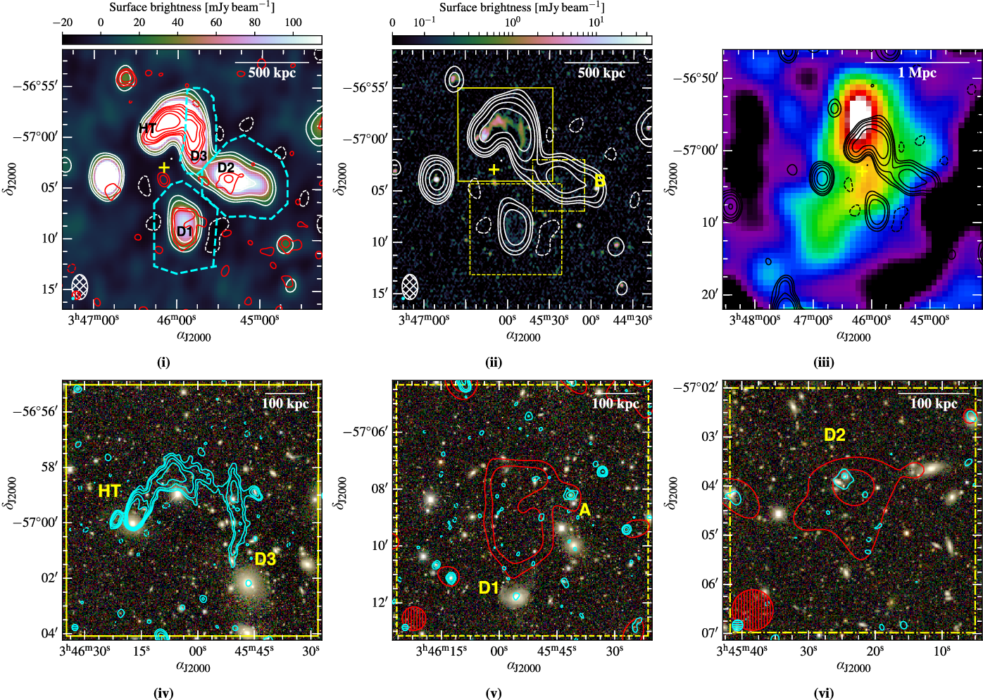
The smoothed RASS image is shown in Figure 21(iii) which highlights a faint X-ray structure detected as the cluster, elongated towards the SE. The X-ray emission does not elucidate the nature of the diffuse components based on location, however, the diffuse emission resides within the clearly elongated X-ray emission to the south of the cluster, thus is in a region where we can assume dynamical activity is occurring.
3.1.9. FIELD11
Abell 3365 (Figure 22). Abell 3365 (RXC J0548.8–2154) was reported to host a relic and candidate second relic by van Weeren et al. (Reference van Weeren, Brüggen, Röttgering, Hoeft, Nuza and Intema2011)—at the time, spectral coverage was minimal. While not in our original survey scope, the cluster resides at the edge of a field that was opportunistically processed for other targets. We show the 154-MHz map in Figure 22 with RACS contours overlaid. The NE relic is detected (D1), and the SW candidate relic source is also detected (D2). An additional extension, labelled D3, is also detected that has not been identified in other radio maps. We utilise the additional spectral coverage offered by the MWA-2 and find, after subtraction of Source A, a power law model for the NE relic, with
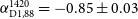 $\alpha _{{\rm{D}}1,88}^{1420} = - 0.85 \pm 0.03$
(Figure 26(xxvii)). We note a curious feature of the flux density measurements wherein the lower MWA bands separate from the higher bands—we cannot explain this feature as either instrumental or physical. While the relic is detected in the RACS data, we note significant negative bowls around the source indicating a lack of flux recovery. A lower limit is provided but not used in fitting. The resultant spectral shape is reasonably shallow for a relic. The SW relic (D2) is detected in MWA-2 data as well, but is too confused in the 88-MHz band. The resultant SED provides
$\alpha _{{\rm{D}}1,88}^{1420} = - 0.85 \pm 0.03$
(Figure 26(xxvii)). We note a curious feature of the flux density measurements wherein the lower MWA bands separate from the higher bands—we cannot explain this feature as either instrumental or physical. While the relic is detected in the RACS data, we note significant negative bowls around the source indicating a lack of flux recovery. A lower limit is provided but not used in fitting. The resultant spectral shape is reasonably shallow for a relic. The SW relic (D2) is detected in MWA-2 data as well, but is too confused in the 88-MHz band. The resultant SED provides
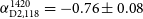 $\alpha _{{\rm{D}}2,118}^{1420} = - 0.76 \pm 0.08$
(Figure 26(xxviii)), noting that the discrete Source A discussed by van Weeren et al. (2011) is not confused in these bands and is not required to be subtracted.
$\alpha _{{\rm{D}}2,118}^{1420} = - 0.76 \pm 0.08$
(Figure 26(xxviii)), noting that the discrete Source A discussed by van Weeren et al. (2011) is not confused in these bands and is not required to be subtracted.
Abell 3365. Background: MWA-2, 154-MHz, robust
 $+1.0$
image. The white contours are as in Figure 2(i) for the background image (with
$+1.0$
image. The white contours are as in Figure 2(i) for the background image (with
 ${\sigma _{{\rm{rms}}}} = 3.5$
mJy beam−1). Red contours: RACS low-resolution,
${\sigma _{{\rm{rms}}}} = 3.5$
mJy beam−1). Red contours: RACS low-resolution,
 $[\pm 3, 6, 12, 24, 48] \times \sigma_{\rm{rms}}$
(
$[\pm 3, 6, 12, 24, 48] \times \sigma_{\rm{rms}}$
(
 $\sigma_{\rm{rms}} = 0.47$
mJy beam−1). Other image features are as in Figures 2 and 3. Note the white circle has a 1 Mpc radius, centred on the coordinates associated with RXC J0548.8–2154 (i.e. the X-ray component for the system).
$\sigma_{\rm{rms}} = 0.47$
mJy beam−1). Other image features are as in Figures 2 and 3. Note the white circle has a 1 Mpc radius, centred on the coordinates associated with RXC J0548.8–2154 (i.e. the X-ray component for the system).
Golovich et al. (Reference Golovich2019) present deep XMM-Newton observations of the cluster along with spectro-optical analysis (see their Fig. 25), highlighting the merger axis and location of the candidate SW relic with respect to three subclusters within the system. They note there is no distinct alignment of the subclusters with the W relic candidate (D2), and given the shallow spectrum we suggest this is not a relic source.
Despite this, Urdampilleta et al. (Reference Urdampilleta, Simionescu, Kaastra, Zhang, Di Gennaro, Mernier, de Plaa and Brunetti2021) find significant temperature jumps across both relics, finding evidence for shocks with Mach numbers
 ${{\cal M}_{{\rm{west}}}} = 3.9 \pm 0.8$
and
${{\cal M}_{{\rm{west}}}} = 3.9 \pm 0.8$
and
 $\mathcal{M}_{\rm{east}} = 3.5 \pm 0.6$
, which for DSA may produce relics with flatter spectral indices as observed here. Assuming DSA for these relics, and assuming
$\mathcal{M}_{\rm{east}} = 3.5 \pm 0.6$
, which for DSA may produce relics with flatter spectral indices as observed here. Assuming DSA for these relics, and assuming
 $\alpha_{\rm{integrated}} = \alpha_{\rm{inj}}$
as might be the case for a re-accelerated fossil electron population (e.g. van Weeren et al. Reference van Weeren2016), we find radio Mach numbers of
$\alpha_{\rm{integrated}} = \alpha_{\rm{inj}}$
as might be the case for a re-accelerated fossil electron population (e.g. van Weeren et al. Reference van Weeren2016), we find radio Mach numbers of
 $\mathcal{M}_{\rm{RW}} = 4.2 \pm 0.4$
and
$\mathcal{M}_{\rm{RW}} = 4.2 \pm 0.4$
and
 $\mathcal{M}_{\rm{RE}} = 2.5 \pm 0.1$
for the western and eastern relics, respectively. If accelerated from the thermal pool, we would expect
$\mathcal{M}_{\rm{RE}} = 2.5 \pm 0.1$
for the western and eastern relics, respectively. If accelerated from the thermal pool, we would expect
 $\alpha_{\rm{inj}} = \alpha_{\rm{integrated}} + 0.5$
, resulting in a non-physical Mach number under standard DSA. The nature of both sources (D1 and D2) is uncertain.
$\alpha_{\rm{inj}} = \alpha_{\rm{integrated}} + 0.5$
, resulting in a non-physical Mach number under standard DSA. The nature of both sources (D1 and D2) is uncertain.
Abell 0550 (Figure 23). We report the detection of a large-scale, elongated emission structure on the periphery of Abell 0550 (Figure 23(i) with an LAS of
 $\sim\!15$
arcmin (
$\sim\!15$
arcmin (
 ${\rm{LLS}}\approx 1.6$
Mpc). We detect the source between 88–154 MHz in the MWA-2 data. We note that there is a spiral galaxy (WISEA J055346.34–211119.6, no redshift) near the centre of the emission, shown in Figure 23(ii), denoted with an ‘S’. Spiral galaxies rarely host large-scale radio lobes, though a small number have been detected, sometimes with remnant lobes (e.g. Hota et al. Reference Hota2011) and this may be such an example. With no compact emission detected in RACS from the spiral galaxy, we can rule out significant AGN contribution and suggest the emission seen in the NVSS and MWA-2 images is related to star-formation processes and that the galaxy, if the host, is not actively fuelling the lobes, consistent with a steep spectrum. The resultant spectrum (Figure 26(xxix)), with the spiral and compact Source A subtracted flattens at 1.4 GHz, and is fit with a generic curved power law, though the physical interpretation of this is not clear. New kpc-scale jets from the spiral that are not subtracted may contribute to the spectral flattening, though this is unlikely to be so extreme and we suggest residual flux from the extended emission from the spiral is affecting the measurements. Across the MWA band we fit a power law model finding a spectral index of
${\rm{LLS}}\approx 1.6$
Mpc). We detect the source between 88–154 MHz in the MWA-2 data. We note that there is a spiral galaxy (WISEA J055346.34–211119.6, no redshift) near the centre of the emission, shown in Figure 23(ii), denoted with an ‘S’. Spiral galaxies rarely host large-scale radio lobes, though a small number have been detected, sometimes with remnant lobes (e.g. Hota et al. Reference Hota2011) and this may be such an example. With no compact emission detected in RACS from the spiral galaxy, we can rule out significant AGN contribution and suggest the emission seen in the NVSS and MWA-2 images is related to star-formation processes and that the galaxy, if the host, is not actively fuelling the lobes, consistent with a steep spectrum. The resultant spectrum (Figure 26(xxix)), with the spiral and compact Source A subtracted flattens at 1.4 GHz, and is fit with a generic curved power law, though the physical interpretation of this is not clear. New kpc-scale jets from the spiral that are not subtracted may contribute to the spectral flattening, though this is unlikely to be so extreme and we suggest residual flux from the extended emission from the spiral is affecting the measurements. Across the MWA band we fit a power law model finding a spectral index of
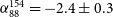 $\alpha_{88}^{154} = -2.4 \pm 0.3$
. Figure 23(iii) shows the emission with respect to the X-ray–emitting core of the cluster, though the source is at the edge of the X-ray data. Bernardi et al. (Reference Bernardi2016) observed the cluster with KAT-7, searching for a central radio halo. This elongated source is outside of their observed FoV but a halo was not detected, and the data here (MWA-2 and re-processed RACS) do not suggest the presence of a halo either.
$\alpha_{88}^{154} = -2.4 \pm 0.3$
. Figure 23(iii) shows the emission with respect to the X-ray–emitting core of the cluster, though the source is at the edge of the X-ray data. Bernardi et al. (Reference Bernardi2016) observed the cluster with KAT-7, searching for a central radio halo. This elongated source is outside of their observed FoV but a halo was not detected, and the data here (MWA-2 and re-processed RACS) do not suggest the presence of a halo either.
Abell 0550. Background: MWA-2, 118-MHz, robust
 $+1.0$
image. (ii) Background: RGB PS1 image (i, r, g). (iii). Background: smoothed XMM-Newton EPIC image. The white contours are as in Figure 2(i) for the background of (i) (with
$+1.0$
image. (ii) Background: RGB PS1 image (i, r, g). (iii). Background: smoothed XMM-Newton EPIC image. The white contours are as in Figure 2(i) for the background of (i) (with
 $\sigma_{\rm{rms}} = 6.6$
mJy beam−1). Red contours: NVSS image,
$\sigma_{\rm{rms}} = 6.6$
mJy beam−1). Red contours: NVSS image,
 $[\pm 3, 6, 12, 24, 48] \times \sigma_{\rm{rms}}$
(
$[\pm 3, 6, 12, 24, 48] \times \sigma_{\rm{rms}}$
(
 $\sigma_{\rm{rms}} = 0.57$
mJy beam−1). Cyan contours: RACS robust
$\sigma_{\rm{rms}} = 0.57$
mJy beam−1). Cyan contours: RACS robust
 $+0.25$
image,
$+0.25$
image,
 $[\pm 3, 6, 12, 24, 48] \times \sigma_{\rm{rms}}$
(
$[\pm 3, 6, 12, 24, 48] \times \sigma_{\rm{rms}}$
(
 $\sigma_{\rm{rms}} = 0.25$
mJy beam−1). Other image features are as in Figure 2 and Figure 3. Note (iii) clips at the location of relic as that is the FoV of the XMM-Newton observation.
$\sigma_{\rm{rms}} = 0.25$
mJy beam−1). Other image features are as in Figure 2 and Figure 3. Note (iii) clips at the location of relic as that is the FoV of the XMM-Newton observation.
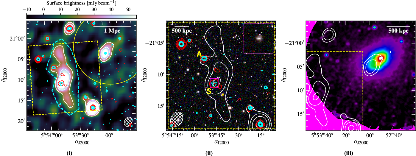
4. Discussion
4.1. Low frequency radio halos and relics
Scaling relationships between diffuse source radio luminosity and cluster properties (e.g.
 $M_{500}$
) have been established for halos, mini-halos, and relics. Recent works have shown that for radio halos these relationships are converging at 1.4 GHz and 150 MHz (Cuciti et al. Reference Cuciti2021; van Weeren et al. Reference van Weeren2020; Duchesne et al. Reference Duchesne, Johnston-Hollitt and Wilber2021c). For relics this is less certain as confirmed radio relic numbers remain low, and scaling relations here typically utilise double relic detections (e.g. de Gasperin et al. Reference de Gasperin, van Weeren, Brüggen, Vazza, Bonafede and Intema2014; de Gasperin et al. Reference de Gasperin, Intema, van Weeren, Dawson, Golovich, Wittman, Bonafede and Brüggen2015; Duchesne et al. Reference Duchesne, Johnston-Hollitt, Bartalucci, Hodgson and Pratt2021a). Similar relationships are found for mini-halos (e.g. Giacintucci et al. Reference Giacintucci, Markevitch, Cassano, Venturi, Clarke, Kale and Cuciti2019; Richard-Laferrière et al. Reference Richard-Laferrière2020), though the effect of the CC on cluster properties (e.g. mass) and contribution of the radio-loud BCG on the estimated mini-halo power may create additional uncertainty in the relations (e.g. Richard-Laferrière et al. Reference Richard-Laferrière2020).
$M_{500}$
) have been established for halos, mini-halos, and relics. Recent works have shown that for radio halos these relationships are converging at 1.4 GHz and 150 MHz (Cuciti et al. Reference Cuciti2021; van Weeren et al. Reference van Weeren2020; Duchesne et al. Reference Duchesne, Johnston-Hollitt and Wilber2021c). For relics this is less certain as confirmed radio relic numbers remain low, and scaling relations here typically utilise double relic detections (e.g. de Gasperin et al. Reference de Gasperin, van Weeren, Brüggen, Vazza, Bonafede and Intema2014; de Gasperin et al. Reference de Gasperin, Intema, van Weeren, Dawson, Golovich, Wittman, Bonafede and Brüggen2015; Duchesne et al. Reference Duchesne, Johnston-Hollitt, Bartalucci, Hodgson and Pratt2021a). Similar relationships are found for mini-halos (e.g. Giacintucci et al. Reference Giacintucci, Markevitch, Cassano, Venturi, Clarke, Kale and Cuciti2019; Richard-Laferrière et al. Reference Richard-Laferrière2020), though the effect of the CC on cluster properties (e.g. mass) and contribution of the radio-loud BCG on the estimated mini-halo power may create additional uncertainty in the relations (e.g. Richard-Laferrière et al. Reference Richard-Laferrière2020).
Despite scatter in these relations, sources in each class tend to stay near the currently determined fits. As a point of comparison, we plot a selection of our sources (namely, candidate halos, relics, and some of the miscellaneous fossil sources) on the
 $P_{v}$
–
$P_{v}$
–
 $M_{500}$
planes to compare against the larger samples. Figure 24 shows these relations for halos (Figure 24(i) and 24(ii)) and relics (Figure 24(iii) and 24(iv)) for
$M_{500}$
planes to compare against the larger samples. Figure 24 shows these relations for halos (Figure 24(i) and 24(ii)) and relics (Figure 24(iii) and 24(iv)) for
 $v \in \{ 150,\,1400\}$
MHz. For each, we plot the best-fit relations from Duchesne et al. (Reference Duchesne, Johnston-Hollitt and Wilber2021c) and Duchesne et al. (Reference Duchesne, Johnston-Hollitt, Bartalucci, Hodgson and Pratt2021a) for halos and relics, respectively. Additionally, the full literature samples used in those works are plotted, and the
$v \in \{ 150,\,1400\}$
MHz. For each, we plot the best-fit relations from Duchesne et al. (Reference Duchesne, Johnston-Hollitt and Wilber2021c) and Duchesne et al. (Reference Duchesne, Johnston-Hollitt, Bartalucci, Hodgson and Pratt2021a) for halos and relics, respectively. Additionally, the full literature samples used in those works are plotted, and the
 $P_{150}$
–
$P_{150}$
–
 $M_{500}$
relation for double relics is scaled from 1400 MHz following Equation 6 from Duchesne et al. (Reference Duchesne, Johnston-Hollitt and Wilber2021c), assuming a mean spectral index of
$M_{500}$
relation for double relics is scaled from 1400 MHz following Equation 6 from Duchesne et al. (Reference Duchesne, Johnston-Hollitt and Wilber2021c), assuming a mean spectral index of
 $\alpha = -1.2$
.
$\alpha = -1.2$
.
Halo and double relic
 $P_{v}$
–
$P_{v}$
–
 $M_{500}$
scaling relations with candidate sources from this work overlaid. Best-fit lines are also shown from Duchesne et al. (Reference Duchesne, Johnston-Hollitt, Bartalucci, Hodgson and Pratt2021a) for relics, with scaling to 150 MHz, and Duchesne et al. (Reference Duchesne, Johnston-Hollitt and Wilber2021c) for halos. Literature data as discussed in Duchesne et al. (Reference Duchesne, Johnston-Hollitt, Bartalucci, Hodgson and Pratt2021a) and Duchesne et al. (Reference Duchesne, Johnston-Hollitt and Wilber2021c) are also shown for reference.
$M_{500}$
scaling relations with candidate sources from this work overlaid. Best-fit lines are also shown from Duchesne et al. (Reference Duchesne, Johnston-Hollitt, Bartalucci, Hodgson and Pratt2021a) for relics, with scaling to 150 MHz, and Duchesne et al. (Reference Duchesne, Johnston-Hollitt and Wilber2021c) for halos. Literature data as discussed in Duchesne et al. (Reference Duchesne, Johnston-Hollitt, Bartalucci, Hodgson and Pratt2021a) and Duchesne et al. (Reference Duchesne, Johnston-Hollitt and Wilber2021c) are also shown for reference.
 $P_{v}|M_{500}$
refers to fits determined assuming
$P_{v}|M_{500}$
refers to fits determined assuming
 $P_{v}$
is the dependent variable and
$P_{v}$
is the dependent variable and
 $M_{500}$
the independent variable, and ‘orthogonal’ refers to an orthogonal regression using the Bivariate Correlated Errors and intrinsic Scatter method (BCES; Akritas & Bershady Reference Akritas and Bershady1996)—see (Duchesne et al. Reference Duchesne, Johnston-Hollitt and Wilber2021c) for further BCES fitting details.
$M_{500}$
the independent variable, and ‘orthogonal’ refers to an orthogonal regression using the Bivariate Correlated Errors and intrinsic Scatter method (BCES; Akritas & Bershady Reference Akritas and Bershady1996)—see (Duchesne et al. Reference Duchesne, Johnston-Hollitt and Wilber2021c) for further BCES fitting details.
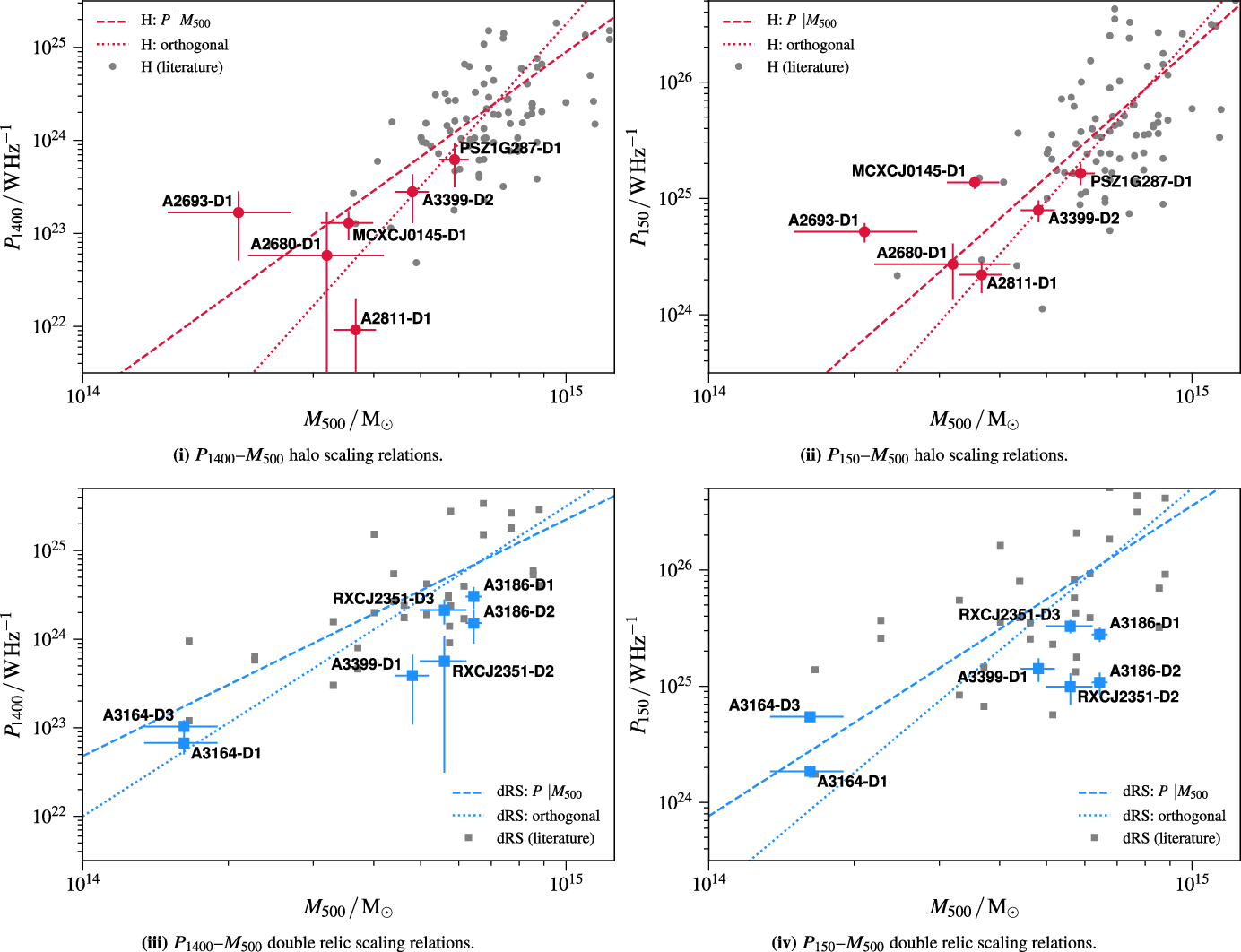
As expected, at 150 MHz the candidate USSRHs in Abell 2811 and PSZ1 G287.95–32.98 shift to be placed on the orthogonal regression line. This is largely consistent with the USSRH population (e.g. Cassano et al. Reference Cassano2013; Bruno et al. Reference Bruno2021; Duchesne et al. Reference Duchesne, Johnston-Hollitt and Wilber2021c) which are normally found to be under-luminous with respect to the 1400 MHz scaling relations but shift towards the regression line when the relation is computed at 150 MHz. Conversely, the candidate halo (or point source) in Abell 2693 sits far above both relations, though the derived mass approaches the limits obtainable with RASS and carries significant uncertainty. Given how few halos are detected in low mass clusters (
 $\lesssim\!5 \times 10^{14}$
M
$\lesssim\!5 \times 10^{14}$
M
 $_\odot$
) and our lack of understanding in this low-mass regime it is difficult to rule out the radio halo classification, however, as discussed previously other characteristics (e.g. location) are less consistent with a halo interpretation. While we suggest the sources in Abell 3164 are fossil plasma sources, their nature is still somewhat uncertain and D1 and D2 are included on Figure 24(iii) and 24(iv) as a reference.
$_\odot$
) and our lack of understanding in this low-mass regime it is difficult to rule out the radio halo classification, however, as discussed previously other characteristics (e.g. location) are less consistent with a halo interpretation. While we suggest the sources in Abell 3164 are fossil plasma sources, their nature is still somewhat uncertain and D1 and D2 are included on Figure 24(iii) and 24(iv) as a reference.
4.2. Clues from integrated spectra—seed electrons & palaeontology
4.2.1. Cluster diffuse sources samples
We find that of the 31 sources reported in this surveyFootnote x , that 13 are likely fossil radio plasma sources: remnant radio galaxies or otherwise remnant outflows from AGN at unknown stages after cessation of an episode of nuclear activity. These sources are labelled ‘F’ and ‘r’ in Table 1. For classification purposes, in Table 1 remnant (‘r’) is used when the morphology still resembles a radio galaxy and when a possible host is identified. These sources are unlikely to be radio halos or relics based on largely morphological and other physical characteristics.
Having established this sample we wish to consider how fossil radio plasmas relate to other diffuse cluster emission. In particular, we wish to consider the question of whether these sources provide a link between the source of electrons in the ICM from which relics and halos may be generated. With the MWA (and ASKAP) we are able to obtain estimates of the spectral index in the MHz regime where most emission models retain power law shapes, and comparisons between different classes of sources (fossils, halos, relics, and remnant radio galaxies) will not be overly effected by spectral curvature.
Table 4 presents details of a literature sample of integrated spectral indices for populations of halos (H), relics (R), mini halos (mH), remnants (r), and cluster-based fossil sources (F), which we compare to our cluster remnant and fossil sample. Where available, we use spectral indices derived from low-frequency measurements (i.e. within the MWA band,
 $\sim\!150$
MHz up to
$\sim\!150$
MHz up to
 $\sim\!1$
GHz).
$\sim\!1$
GHz).
Median spectral indices for the diffuse source populations.
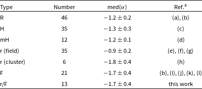
Samples drawn from: (a) Duchesne et al. (Reference Duchesne, Johnston-Hollitt, Bartalucci, Hodgson and Pratt2021a); (b) van Weeren et al. (Reference van Weeren, de Gasperin, Akamatsu, Brüggen, Feretti, Kang, Stroe and Zandanel2019); (c) Duchesne et al. (Reference Duchesne, Johnston-Hollitt and Wilber2021c); (d) Richard-Laferrière et al. (Reference Richard-Laferrière2020); (e) Brienza et al. (Reference Brienza2017); (f) Mahatma et al. (Reference Mahatma2018); (g) Quici et al. (Reference Quici2021); (h) Murgia et al. (Reference Murgia2011); (i) Duchesne et al. (Reference Duchesne, Johnston-Hollitt, Zhu, Wayth and Line2020); (j) Mandal et al. (Reference Mandal2020); (k) Giacintucci et al. (Reference Giacintucci, Markevitch, Johnston-Hollitt, Wik, Wang and Clarke2020); (l) Hodgson et al. (Reference Hodgson, Bartalucci, Johnston-Hollitt, McKinley, Vazza and Wittor2021).
Spectral indices have been derived from a variety of measurements/instruments and spectra may steepen (if a low-frequency observation is more sensitive; e.g. Macario et al. Reference Macario, Venturi, Brunetti, Dallacasa, Giacintucci, Cassano, Bardelli and Athreya2010) or flatten (if a high-frequency observation is more sensitive; e.g. Ogrean et al. Reference Ogrean2015) artificially due to a mismatch of u,v sampling and general sensitivity between observations. This introduces further uncertainty to the spectral indices, but is not likely to bias the distributions significantly towards steeper or flatter spectra.
We show the histograms of reported
 $\alpha$
in Figure 25 for our sample of cluster fossil plasma sources (r and F in Table 1) against three classes of objects from the samples described in Table 4: i) halos and mini halos, ii) relics (both single and double systems), and iii) cluster fossils sources and both field and cluster remnants.
$\alpha$
in Figure 25 for our sample of cluster fossil plasma sources (r and F in Table 1) against three classes of objects from the samples described in Table 4: i) halos and mini halos, ii) relics (both single and double systems), and iii) cluster fossils sources and both field and cluster remnants.
Spectral index distributions for (i) radio halos, (ii) relics (double and single), and (iii) remnant radio galaxies and fossil radio plasma sources, compared to the collection of fossils plasma sources reported in this work. See Section 4.2 and Table 4 for population details. Vertical lines indicate median population values. Note that bins are clipped at
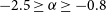 $-2.5 \geq \alpha \geq -0.8$
, and our sample is generally clipped at
$-2.5 \geq \alpha \geq -0.8$
, and our sample is generally clipped at
 $\sim\! -0.9$
by construction due to the original search criteria.
$\sim\! -0.9$
by construction due to the original search criteria.
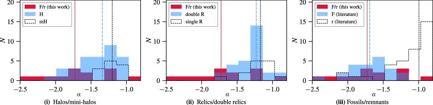
Median
 $\alpha$
obtained for each distribution are reported in Table 4. We note the single relic population is unlikely to be fundamentally different to the double relic population, which are thought to form through the same shock-acceleration processes. This is evident in Figure 25(ii) which shows the distribution of
$\alpha$
obtained for each distribution are reported in Table 4. We note the single relic population is unlikely to be fundamentally different to the double relic population, which are thought to form through the same shock-acceleration processes. This is evident in Figure 25(ii) which shows the distribution of
 $\alpha$
is not significantly different between the two samples. Furthermore, the halo and relic median spectral indices are consistent, suggesting a common generation time if drawn from the same underlying electron population (though as discussed previously the generation mechanisms are thought to be different, but both associated with mergers). We note that the radio halo sample shown in Figure 25(i) includes USSRHs as expected from turbulent (re-)acceleration processes which creates a significant tail in the distribution towards steeper spectra. Relics show a similar ultra-steep–spectrum tail but are much more densely peaked around their median value.
$\alpha$
is not significantly different between the two samples. Furthermore, the halo and relic median spectral indices are consistent, suggesting a common generation time if drawn from the same underlying electron population (though as discussed previously the generation mechanisms are thought to be different, but both associated with mergers). We note that the radio halo sample shown in Figure 25(i) includes USSRHs as expected from turbulent (re-)acceleration processes which creates a significant tail in the distribution towards steeper spectra. Relics show a similar ultra-steep–spectrum tail but are much more densely peaked around their median value.
4.2.2. Remnants, fossils, and revived radio plasma: seed electron populations?
Figure 25 shows that, in general, fossil plasma sources tend towards steeper spectra than the relic and halo populations, and are significantly steeper than field remnant radio galaxies. The few remnants found in clusters (e.g. Murgia et al. Reference Murgia2011) typically have steeper spectra at equivalent frequencies than their field counterpartsFootnote y . Sources such as D1 in Abell S1099 may represent a younger cluster remnant, and with no evidence of morphological disturbance of the ICM we do not consider this a re-accelerated source. It is likely the cluster environment plays a role in allowing these sources to remain visible for longer (e.g. by constraining diffusion of the electrons into the surrounding ICM; Murgia et al. Reference Murgia2011). Studies (Brienza et al. Reference Brienza2017; Mahatma et al. Reference Mahatma2018; Jurlin et al. Reference Jurlin2020; Quici et al. Reference Quici2021) suggest remnants have a short observable lifetime before surface brightness becomes prohibitively faint as the plasma both steepens in spectrum and expands. With low numbers of these remnant and fossil sources, it is difficult to draw firm conclusions about the role of the cluster environment.
Given the ubiquity of radio galaxies of complex morphologies in clusters (e.g. Hardcastle & Sakelliou Reference Hardcastle and Sakelliou2004; Clarke & Ensslin Reference Clarke and Ensslin2006; Sakelliou et al. Reference Sakelliou, Hardcastle and Jetha2008; Botteon et al. Reference Botteon2020c; Brüggen et al. Reference Brüggen2021) we expect a large population of these fossil plasma sources waiting to be re-accelerated by merger-based shocks and turbulence. By construction, we have steep-spectrum (and ultra-steep–spectrum) sources in either relaxed, or ‘ambiguously dynamic’ clusters that cannot be described as relics or halos—these are likely fossil radio plasma and highlight a population of sources in clusters that can provide seed electrons for relic and halo sources as well as smaller-scale revived fossil plasma like phoenices.
Examples exist in the literature of re-acceleration of fossil plasmas with some connection to AGN (e.g. Bonafede et al. Reference Bonafede, Intema, Brüggen, Girardi, Nonino, Kantharia, van Weeren and Röttgering2014; van Weeren et al. Reference van Weeren2017; de Gasperin Reference de Gasperin2017; Wilber et al. Reference Wilber2019), and simulations have shown that fossil electrons from AGN outflows and long-dead radio galaxies can (1) exist diffusively within the ICM (Vazza et al. Reference Vazza, Wittor, Brunetti and Brüggen2021) and (2) be re-accelerated by normal DSA-like processes (e.g. Kang Reference Kang2018). It is not clear that the acceleration efficiency for electrons at shocks is sufficient to produce the observed relics unless there is a mildly-relativistic population (e.g. Botteon et al. Reference Botteon, Brunetti, Ryu and Roh2020b), though many observed properties of relics do not require a population of fossil electrons (e.g. Rajpurohit et al. Reference Rajpurohit2020; Rajpurohit et al. Reference Rajpurohit2021b). The distribution of
 $\alpha$
for relics and halos extends into the ultra-steep–spectrum regime which would be consistent with a population of re-accelerated fossil electrons in low-energy events (e.g. from weak mergers triggering USSRH; Brunetti et al. Reference Brunetti2008), though it is not clear whether the density of such a fossil electron population would be sufficient to produce the observed emission. In general, such weaker events should be more common and simulations suggest a large population of faint diffuse sources should exist (e.g. Nuza et al. Reference Nuza, Hoeft, van Weeren, Gottlöber and Yepes2012); however, these low surface brightness and ultra-steep spectrum sources are still challenging to detect and image. Surveys with e.g. LOFAR (especially combining HBA and LBA data for spectral information) should uncover a larger number of these ultra-steep–spectrum sources and indeed instruments like MWA, LOFAR, and the uGMRT are now starting to uncover them (e.g. Giacintucci et al. Reference Giacintucci, Markevitch, Johnston-Hollitt, Wik, Wang and Clarke2020; Mandal et al. Reference Mandal2020; Hodgson et al. Reference Hodgson, Bartalucci, Johnston-Hollitt, McKinley, Vazza and Wittor2021).
$\alpha$
for relics and halos extends into the ultra-steep–spectrum regime which would be consistent with a population of re-accelerated fossil electrons in low-energy events (e.g. from weak mergers triggering USSRH; Brunetti et al. Reference Brunetti2008), though it is not clear whether the density of such a fossil electron population would be sufficient to produce the observed emission. In general, such weaker events should be more common and simulations suggest a large population of faint diffuse sources should exist (e.g. Nuza et al. Reference Nuza, Hoeft, van Weeren, Gottlöber and Yepes2012); however, these low surface brightness and ultra-steep spectrum sources are still challenging to detect and image. Surveys with e.g. LOFAR (especially combining HBA and LBA data for spectral information) should uncover a larger number of these ultra-steep–spectrum sources and indeed instruments like MWA, LOFAR, and the uGMRT are now starting to uncover them (e.g. Giacintucci et al. Reference Giacintucci, Markevitch, Johnston-Hollitt, Wik, Wang and Clarke2020; Mandal et al. Reference Mandal2020; Hodgson et al. Reference Hodgson, Bartalucci, Johnston-Hollitt, McKinley, Vazza and Wittor2021).
5. Summary
In this work we have reported an MWA-2 follow-up survey of candidate diffuse cluster radio sources originally detected in MWA Phase I data as part of the GLEAM survey and EoR0 field survey D21. We have combined the MWA-2 data with recent ASKAP data at 887 MHz to (1) attempt to classify the sources based on their morphologies, host cluster properties, and SEDs and (2) simply ensure sources are not confused point sources—an ongoing problem with low-resolution interferometric observations. We report on 31 sources, with 6 candidate halos, 2 mini-halos (1 candidate), 3 relics (1 candidate and 1 double relic system), 13 remnant AGN or miscellaneous fossil plasmas. Some of the candidate sources are found to be point sources or radio galaxies, and we also follow-up the ‘twin relic’ in Abell 0168 reported by Dwarakanath et al. (Reference Dwarakanath, Parekh, Kale and George2018) and the double-relic system in Abell 3365 reported by van Weeren et al. (Reference van Weeren, Brüggen, Röttgering, Hoeft, Nuza and Intema2011). Specifically, we report the detection of a new double relic system associated with Abell 3186, a mini-halo associated with RXC J0137.2–0912 and that the candidate halo in Abell 2811 reported by D21 has a spectral index of
 $\alpha = -2.5\pm0.4$
, though this will require follow-up high resolution, high-sensitivity observations to confirm its nature. We also observe an HT galaxy in Abell 3164 that exhibits episodic activity with a potentially re-accelerated component.
$\alpha = -2.5\pm0.4$
, though this will require follow-up high resolution, high-sensitivity observations to confirm its nature. We also observe an HT galaxy in Abell 3164 that exhibits episodic activity with a potentially re-accelerated component.
We find that generally the relics and halos presented here sit in reasonable locations on the established
 $P_{1400}$
–
$P_{1400}$
–
 $M_{500}$
and
$M_{500}$
and
 $P_{150}$
–
$P_{150}$
–
 $M_{500}$
scaling relations, with the USSRHs shifting closer towards the
$M_{500}$
scaling relations, with the USSRHs shifting closer towards the
 $P_{150}$
–
$P_{150}$
–
 $M_{500}$
relation. We also compare the integrated spectra of our sample of cluster fossil and remnant sources against various samples of steep-spectrum, diffuse cluster sources as well as field remnant radio galaxies, finding that the general spectral properties are consistent with the literature fossil radio source population. This is in turn consistent with the integrated, low-frequency spectral indices of cluster-based remnant radio galaxies. We have discussed the putative link between these fossil sources and other diffuse cluster sources, noting that the distributions of spectral indices for diffuse clusters sources would be consistent with fossil radio plasmas as seed electrons for the emission.
$M_{500}$
relation. We also compare the integrated spectra of our sample of cluster fossil and remnant sources against various samples of steep-spectrum, diffuse cluster sources as well as field remnant radio galaxies, finding that the general spectral properties are consistent with the literature fossil radio source population. This is in turn consistent with the integrated, low-frequency spectral indices of cluster-based remnant radio galaxies. We have discussed the putative link between these fossil sources and other diffuse cluster sources, noting that the distributions of spectral indices for diffuse clusters sources would be consistent with fossil radio plasmas as seed electrons for the emission.
In this work we have just gently brushed the dust off of a small collection of old fossils and large-scale, deep, and high-resolution surveys with the SKA pathfinders—particularly ASKAP and MeerKAT with
 $\sim\!5$
–15 arcsec resolution over the Southern Sky—will enable high-fidelity follow-up of these types of sources placing constraints on the
$\sim\!5$
–15 arcsec resolution over the Southern Sky—will enable high-fidelity follow-up of these types of sources placing constraints on the
 $\gtrsim 1$
GHz spectrum. In the future SKA should dig deeper, revealing myriad new ultra-steep spectrum radio fossils, providing key observational evidence for any link between these sources and cluster halos and relics.
$\gtrsim 1$
GHz spectrum. In the future SKA should dig deeper, revealing myriad new ultra-steep spectrum radio fossils, providing key observational evidence for any link between these sources and cluster halos and relics.
Acknowledgements
The authors would like to thank Dr. Paula Tarro Alonso for providing mass estimates for Abell 2680 and Abell 2693. SWD acknowledges an Australian Government Research Training Program scholarship administered through Curtin University. The Australian SKA Pathfinder is part of the Australia Telescope National Facility which is managed by CSIRO. Operation of ASKAP is funded by the Australian Government with support from the National Collaborative Research Infrastructure Strategy. ASKAP uses the resources of the Pawsey Supercomputing Centre. Establishment of ASKAP, the Murchison Radio-astronomy Observatory and the Pawsey Supercomputing Centre are initiatives of the Australian Government, with support from the Government of Western Australia and the Science and Industry Endowment Fund. We acknowledge the Wajarri Yamatji people as the traditional owners of the Observatory site. Support for the operation of the MWA is provided by the Australian Government (NCRIS), under a contract to Curtin University administered by Astronomy Australia Limited. This research has made use of data obtained from the Chandra Data Archive and the Chandra Source Catalog, and software provided by the Chandra X-ray Center (CXC) in the application package CIAO. This research has made use of the NASA/IPAC Extragalactic Database (NED), which is operated by the Jet Propulsion Laboratory, California Institute of Technology, under contract with the National Aeronautics and Space Administration. This research has made use of the VizieR catalogue access tool, CDS, Strasbourg, France. The original description of the VizieR service was described in Ochsenbein et al. (Reference Ochsenbein, Bauer and Marcout2000).
This research made use of a number of python packages not explicitly mentioned in the main text: aplpy (Robitaille & Bressert Reference Robitaille and Bressert2012), astropy (Astropy Collaboration et al. Reference Astropy2013), matplotlib (Hunter Reference Hunter2007), numpy (van der Walt et al. Reference van der Walt, Colbert and Varoquaux2011) and scipy (Jones et al. Reference Jones, Oliphant and Peterson2001).
A. Non-candidates
In this section we will record clusters previously reported as having candidate diffuse emission by D21 but are shown by the MWA-2 data to be discrete sources. Note that while FIELD1 and FIELD2 overlap with a majority image used by Duchesne et al. Reference Duchesne, Johnston-Hollitt, Offringa, Pratt, Zheng and Dehghan2021b, for some clusters towards the edges of the fields we are unable to confirm the presence of either diffuse emission of discrete sources—these clusters are not mentioned here.
Abell 0022 Edge of image. Inconclusive.
Abell 0033 Edge of image. Inconclusive.
Abell 2798 Resolution still not sufficient. Inconclusive.
Abell S1136 To be discussed in Macgregor et al. (in prepatation).
Abell S1063 Halo reported by Xie et al. (Reference Xie2020).
Abell 2556 The MWA-2 216-MHz, robust
 $+0.5$
image breaks up into three discrete point sources. RACS data confirm the source is a number of point sources and a double-lobed radio galaxy, with a spectral index
$+0.5$
image breaks up into three discrete point sources. RACS data confirm the source is a number of point sources and a double-lobed radio galaxy, with a spectral index
 $\alpha \sim -0.8$
. The steeper spectral index reported by D21 is a result of point sources contributing to the 168-MHz measurement but not the 1.4-GHz measurement.
$\alpha \sim -0.8$
. The steeper spectral index reported by D21 is a result of point sources contributing to the 168-MHz measurement but not the 1.4-GHz measurement.
Abell S0084 MWA-2 data breaks into two discrete components and RACS confirms this. We cannot confirm the candidate halo/mini-halo.
Abell S1121 Out of images.
PSZ G082.31–67.01 Out of images.
B. Measured source properties
A table of measured and derived source properties are provided for all frequencies (88, 118, 154, 169, 185, 200, 216, 887, 943, and 1400 MHz, though note not all sources are measured at every frequency) as supplementary online material available at the datastore for the Publications of the Astronomical Society of Australia, hosted at https://dx.doi.org/10.26185/611f33b774e96. The following details the columns available for each source:
-
C0 cluster_name
Name of cluster as it appears in Table 1.
-
C1 source_id
ID of source as used in Section 3.1 and in figures.
-
C2 flux_$nu (mJy)
Final flux density of source at frequency $nu MHz.
-
C3 err_flux_$nu (mJy)
Uncertainty on the final flux density of source at frequency $nu MHz.
-
C4 conf_$nu (mJy)
Total confusing flux density subtracted from initial measurement at frequency $nu MHz.
-
C5 err_conf_$nu (mJy)
Uncertainty on total confusing flux density subtracted from initial measurement at frequency $nu MHz. This is added in quadrature to the initial measurement.
-
C6 psf_a_$nu (arcsec)
FWHM of PSF major axis in $nu-MHz image at the source location.
-
C7 psf_b_$nu (arcsec)
FWHM of PSF minor axis in $nu-MHz image at the source location.
 $\vdots$
-
C56 alpha_mwa
Spectral index across the MWA-2 images as shown in Figure 26(i)–(xxix).
-
C57 alpha
Spectral index across all data for power law models as shown in Figure 26(i)–(xxix).
-
C58 q
Curvature parameter for curved power law model fits (Eq. 6), as shown in Figure 26(i)–(xxix).

Integrated spectra of diffuse sources described in Section 3.1 in the order they are reported. The ordinate and abscissa are integrated flux density (mJy) and frequency (MHz), respectively. Individual measurements are reported in the online table described in Appendix B. The dashed, black lines are the fits for the full set of measurements (with grey, shaded regions corresponding to 95% confidence intervals) and the red, dotted lines are fits for only the MWA-2 data. Note black arrows represent limits. Note if only two data points are available, a two-point spectral index was calculated and the resultant line is drawn based on that spectral index. For curved power law spectra, we report the curvature, q, rather than the equivalent spectral index.

C. Integrated spectra
Figure 26(i)–(xxix) show the SEDs for all sources reported in Section 3.1. For each source with MWA-2 and additional data, we additionally provide a power law fit to the MWA-2 data only.
D. Flux recovery in MWA-2 data
Figure 27(i)–(ix) show the ratios of dirty to CLEAN flux density for Gaussian models of varying FWHM. For each source the residual flux density is integrated and multiplied by the factor
 $S_{\rm{CLEAN}} / S_{\rm{dirty}}$
to account for this. Additional detail of this process is provided in Duchesne et al. (Reference Duchesne, Johnston-Hollitt and Wilber2021c).
$S_{\rm{CLEAN}} / S_{\rm{dirty}}$
to account for this. Additional detail of this process is provided in Duchesne et al. (Reference Duchesne, Johnston-Hollitt and Wilber2021c).
Flux recovery and ratio of deconvolved (‘CLEAN’) to un-deconvolved (‘dirty’) integrated flux density for individual snapshots (grey lines). The angular scale on the abscissa correspond to FWHM of the simulated Gaussian (sampled every 30 arcsec). The mean profile,
 $\overline{S_{\rm{dirty}} / S_{\rm{CLEAN}}}$
, is plotted with the standard deviation plotted as a red shaded region. The mean peak flux profile,
$\overline{S_{\rm{dirty}} / S_{\rm{CLEAN}}}$
, is plotted with the standard deviation plotted as a red shaded region. The mean peak flux profile,
 $\overline{S_{p,{\rm{dirty}}} / S_{p,{\rm{CLEAN}}}}$
, is also shown. (i) and (vi) are re-produced from Duchesne et al. (Reference Duchesne, Johnston-Hollitt and Wilber2021c) for completeness.
$\overline{S_{p,{\rm{dirty}}} / S_{p,{\rm{CLEAN}}}}$
, is also shown. (i) and (vi) are re-produced from Duchesne et al. (Reference Duchesne, Johnston-Hollitt and Wilber2021c) for completeness.