





1 Introduction
1.1 Motivation
Our motivation arises from the Generalized Riemann Hypothesis (GRH). A well-known consequence of GRH is that the least quadratic non-residue modulo a prime p is bounded above by
$(\log p)^2$
 . While this ensures the existence of quadratic non-residues in intervals of size
$(\log p)^A$
. While this ensures the existence of quadratic non-residues in intervals of size
$(\log p)^A$
 when
$A> 2$
when
$A> 2$
 , far less is known about their behavior in shorter intervals such as
$[1, (\log p)^A]$
, far less is known about their behavior in shorter intervals such as
$[1, (\log p)^A]$
 for any fixed
$A> 0$
for any fixed
$A> 0$
 .
.
In this article, we investigate the arithmetic nature of such small quadratic non-residues in the context of partitions. Inspired by the classical work of Erdős and Lehner [Reference Erdős and Lehner17], who studied the statistical distribution of partitions in which no summand exceeds a given threshold, we consider partitions where the parts are small prime quadratic non-residues modulo p and study their statistical properties for almost all primes p.
Our goals in this article are threefold. First, we establish distributional results for partitions whose parts are prime quadratic non-residues modulo p and are contained in intervals of the form
$[1, (\log p)^A]$
 . Second, we go beyond the GRH barrier by proving such results even when
$A \in (0,2]$
. Second, we go beyond the GRH barrier by proving such results even when
$A \in (0,2]$
 , and do so unconditionally. Third, we extend our results to accommodate broader frameworks where the parts have additional arithmetic constraints, such as character twists, Möbius twists, and arithmetic progressions.
1.2 Survey of previous results
For an odd prime
$ p $
 , let
$ n_p $
, let
$ n_p $
 denote the least quadratic non-residue modulo
$ p $
denote the least quadratic non-residue modulo
$ p $
 . Using the Pólya–Vinogradov inequality, Vinogradov showed that
$ n_p \ll p^{1/(2\sqrt {e})} (\log p)^2 $
. Using the Pólya–Vinogradov inequality, Vinogradov showed that
$ n_p \ll p^{1/(2\sqrt {e})} (\log p)^2 $
 . He further conjectured that
$ n_p \ll _\varepsilon p^\varepsilon $
. He further conjectured that
$ n_p \ll _\varepsilon p^\varepsilon $
 for any
$ \varepsilon> 0 $
for any
$ \varepsilon> 0 $
 . Currently, the best known upper bound
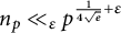
for any fixed
$\varepsilon>0$
 is due to Burgess [Reference Burgess10]. Assuming GRH, Ankeny [Reference Ankeny2] showed that
$n_p \ll (\log p)^2$
is due to Burgess [Reference Burgess10]. Assuming GRH, Ankeny [Reference Ankeny2] showed that
$n_p \ll (\log p)^2$
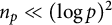 . Lamzouri, Li, and Soundararajan [Reference Lamzouri, Li and Soundararajan28] made Ankeny’s bound explicit by showing that
$n_p\leq (\log p)^2$
. Lamzouri, Li, and Soundararajan [Reference Lamzouri, Li and Soundararajan28] made Ankeny’s bound explicit by showing that
$n_p\leq (\log p)^2$
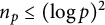 under GRH. See Carniero–Milinovich–Quesada-Herrera–Ramos [Reference Carneiro, Milinovich, Quesada-Herrera and Ramos11] for improvements to the leading constant in this inequality.
For results concerning almost all primes, Linnik [Reference Linnik30] used the large sieve to show that for any fixed
$\varepsilon> 0$
 , almost all primes
$p\leq X$
, almost all primes
$p\leq X$
 satisfy
$n_p\ll _{\varepsilon } p^{\varepsilon }$
satisfy
$n_p\ll _{\varepsilon } p^{\varepsilon }$
 . More precisely, he showed that

Furthermore, by applying Linnik’s technique alongside mean-value estimates for quadratic characters (see [Reference Baier3, Reference Duke and Kowalski15]), one can obtain sharp estimates of the form

for any fixed
$A>1$
 .
.
To study small quadratic non-residues, a natural approach is to study quadratic character sums over short intervals. A classical result of Davenport and Erdős [Reference Davenport and Erdös13] shows that for each prime p, quadratic character sums over short moving intervals across the full range
$[1, p]$
 exhibit Gaussian distribution under certain limiting conditions. This result was extended by Lamzouri [Reference Lamzouri27] to more general Dirichlet characters and exponential sums. In a different direction, it was shown in [Reference Basak, Nath and Zaharescu5] that for almost all primes p, if the short moving intervals are restricted to the initial range
$[1, (\log p)^A]$
exhibit Gaussian distribution under certain limiting conditions. This result was extended by Lamzouri [Reference Lamzouri27] to more general Dirichlet characters and exponential sums. In a different direction, it was shown in [Reference Basak, Nath and Zaharescu5] that for almost all primes p, if the short moving intervals are restricted to the initial range
$[1, (\log p)^A]$
 for any
$A> 1$
for any
$A> 1$
 , the distribution is still Gaussian. Furthermore, in [Reference Basak, Nath and Zaharescu6], it was shown that for
$A> 2$
, the distribution is still Gaussian. Furthermore, in [Reference Basak, Nath and Zaharescu6], it was shown that for
$A> 2$
 , the sequence of consecutive small quadratic non-residues exhibits Poisson behavior.
In this article, we are interested in studying the behavior of small quadratic non-residues in the context of partitions. A partition of a positive integer m is a non-decreasing sequence of positive integers whose sum is equal to m. Let
$\mathcal {P}(m)$
 Footnote
1
denote the number of partitions of m. Asymptotic estimates for
$\mathcal {P}(m)$
Footnote
1
denote the number of partitions of m. Asymptotic estimates for
$\mathcal {P}(m)$
 were first obtained by Hardy and Ramanujan [Reference Hardy and Ramanujan22], where they proved that

Beyond this asymptotic formula, they introduced the Hardy–Ramanujan circle method, which uses modular transformations to derive a divergent series for
$\mathcal {P}(m)$
 with remarkably small error. This method was later refined by Rademacher [Reference Rademacher36], who succeeded in obtaining a convergent series representation for
$\mathcal {P}(m)$
with remarkably small error. This method was later refined by Rademacher [Reference Rademacher36], who succeeded in obtaining a convergent series representation for
$\mathcal {P}(m)$
 . Independently, Ingham [Reference Ingham25] showed that the asymptotic formula (1.1) can also be deduced via a Tauberian theorem.
Given a subset
$\mathbb {A} \subset \mathbb {N}$
 , let
$\mathcal {P}_{\mathbb {A}}(m)$
, let
$\mathcal {P}_{\mathbb {A}}(m)$
 denote the number of partitions of m with all parts belonging to
$\mathbb {A}$
denote the number of partitions of m with all parts belonging to
$\mathbb {A}$
 . The function
$\mathcal {P}_{\mathbb {A}}(m)$
. The function
$\mathcal {P}_{\mathbb {A}}(m)$
 has been the subject of extensive study under diverse arithmetic and combinatorial constraints. In their seminal work [Reference Erdős and Lehner17], Erdős and Lehner studied the distribution of
$\mathcal {P}_{\mathbb {A}}(m)$
has been the subject of extensive study under diverse arithmetic and combinatorial constraints. In their seminal work [Reference Erdős and Lehner17], Erdős and Lehner studied the distribution of
$\mathcal {P}_{\mathbb {A}}(m)$
 in the special case where
$\mathbb {A}$
in the special case where
$\mathbb {A}$
 is the set of the first K positive integers, uniformly for
$K = o(m^{\frac {1}{3}})$
is the set of the first K positive integers, uniformly for
$K = o(m^{\frac {1}{3}})$
 . More precisely, they showed that if
$K=C^{-1}m^{\frac {1}{2}} \log m +xm^{\frac {1}{2}}$
. More precisely, they showed that if
$K=C^{-1}m^{\frac {1}{2}} \log m +xm^{\frac {1}{2}}$
 with
$C=\pi \sqrt {2/3}$
with
$C=\pi \sqrt {2/3}$
 , then

where
$\mathbb {A}= [1,K]$
 . We also highlight classical works of Lehner [Reference Lehner29], Petersson [Reference Petersson35], Livingood [Reference Livingood31], and Grosswald [Reference Grosswald21], among others, which provide asymptotic estimates and exact formulas for
$\mathcal {P}_{\mathbb {A}}(m)$
. We also highlight classical works of Lehner [Reference Lehner29], Petersson [Reference Petersson35], Livingood [Reference Livingood31], and Grosswald [Reference Grosswald21], among others, which provide asymptotic estimates and exact formulas for
$\mathcal {P}_{\mathbb {A}}(m)$
 pertaining to subsets
$\mathbb {A} \subseteq \mathbb {Z}/q\mathbb {Z}$
pertaining to subsets
$\mathbb {A} \subseteq \mathbb {Z}/q\mathbb {Z}$
 for a fixed prime q. More recently, Vaughan [Reference Vaughan40] established asymptotic estimates for
$\mathcal {P}_{\mathbb {A}}(m)$
for a fixed prime q. More recently, Vaughan [Reference Vaughan40] established asymptotic estimates for
$\mathcal {P}_{\mathbb {A}}(m)$
 , where
$\mathbb {A}$
, where
$\mathbb {A}$
 is the set of primes. Vaughan’s method has since been extended to accommodate other special classes of subsets
$\mathbb {A}$
is the set of primes. Vaughan’s method has since been extended to accommodate other special classes of subsets
$\mathbb {A}$
 (see, e.g., [Reference Berndt, Malik and Zaharescu8, Reference Dunn and Robles16, Reference Gafni18, Reference Gafni19] and the references therein). Finally, we also mention the works [Reference Basak, Goldfeld, Heap, Robles and Zaharescu4, Reference Basak, Robles and Zaharescu7] in which certain partition structures were studied for sets
$\mathbb {A}$
(see, e.g., [Reference Berndt, Malik and Zaharescu8, Reference Dunn and Robles16, Reference Gafni18, Reference Gafni19] and the references therein). Finally, we also mention the works [Reference Basak, Goldfeld, Heap, Robles and Zaharescu4, Reference Basak, Robles and Zaharescu7] in which certain partition structures were studied for sets
$\mathbb {A}$
 endowed with an associated oscillatory sequence, such as the Möbius function or quadratic characters.
Meinardus [Reference Meinardus32] established asymptotic estimates for
$\mathcal {P}_{\mathbb {A}}(m)$
 for general subsets
$\mathbb {A} \subset \mathbb {N}$
for general subsets
$\mathbb {A} \subset \mathbb {N}$
 , under certain analytic conditions on the associated zeta functions. More recently, Meinardus’ results have been generalized to broader settings under weaker assumptions by Debruyne–Tenenbaum [Reference Debruyne and Tenenbaum14] and Bridges–Brindle–Bringmann–Franke [Reference Bridges, Brindle, Bringmann and Franke9] by using the saddle point method. Finally, we also mention that Nathanson [Reference Nathanson34] obtained asymptotic estimates for
$\mathcal {P}_{\mathbb {A}}(m)$
, under certain analytic conditions on the associated zeta functions. More recently, Meinardus’ results have been generalized to broader settings under weaker assumptions by Debruyne–Tenenbaum [Reference Debruyne and Tenenbaum14] and Bridges–Brindle–Bringmann–Franke [Reference Bridges, Brindle, Bringmann and Franke9] by using the saddle point method. Finally, we also mention that Nathanson [Reference Nathanson34] obtained asymptotic estimates for
$\mathcal {P}_{\mathbb {A}}(m)$
 accompanied by error terms, where
$\mathbb {A}$
accompanied by error terms, where
$\mathbb {A}$
 is a non-empty finite set of relatively prime positive integers.
Our objective in this work is to consider partitions where each part is a small prime quadratic non-residue modulo a large prime p. As we shall see, the sets
$\mathbb {A}$
 arising in our setting do not satisfy the analytic conditions required for the methods developed in [Reference Bridges, Brindle, Bringmann and Franke9, Reference Debruyne and Tenenbaum14, Reference Meinardus32]. Moreover, our analysis departs significantly from earlier works of Lehner [Reference Lehner29] and Grosswald [Reference Grosswald21], where the modulus q is fixed and the parameter m is large. Nathanson’s asymptotic formula is also restricted to parts that are of bounded size, which will not be the case in our setting. Therefore, a different approach is required that blends analytic and combinatorial methods tailored to the specific structure of small prime quadratic non-residues. In Section 2, we will provide a more detailed discussion comparing our methods with previous works. We now turn to a precise description of our main results.
1.3 Statement of the main results
To state our main results, we require some notation. Throughout the article, we let
$X>0$
 be sufficiently large, depending on other parameters which will be specified as necessary. Let
$A>0$
be sufficiently large, depending on other parameters which will be specified as necessary. Let
$A>0$
 be an arbitrary constant and set
$K=(\log X)^A$
be an arbitrary constant and set
$K=(\log X)^A$
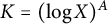 . For each prime
$p \in (X,2X]$
. For each prime
$p \in (X,2X]$
 , we define

where
$(\frac {\cdot }{p})$
 is the Legendre symbol modulo p. Let

For clarity, we mention here that
$\{a_{k,p} \}$
 ,
$\mathbb {H}_p$
,
$\mathbb {H}_p$
 , and
$H_p$
, and
$H_p$
 also depend on X and A, but for brevity, we suppress this in the notation. For
$w \in \mathbb {C}$
also depend on X and A, but for brevity, we suppress this in the notation. For
$w \in \mathbb {C}$
 with
$\lvert w \rvert <1$
with
$\lvert w \rvert <1$
 , consider the generating function

Then
$\mathcal {P}_{\mathbb {H}_p}(m)$
 represents the number of partitions of a positive integer
$ m $
represents the number of partitions of a positive integer
$ m $
 into parts that are prime quadratic non-residues modulo
$ p $
into parts that are prime quadratic non-residues modulo
$ p $
 and do not exceed
$(\log X)^A$
and do not exceed
$(\log X)^A$
 . In other words,
$\mathcal {P}_{\mathbb {H}_p}(m)$
. In other words,
$\mathcal {P}_{\mathbb {H}_p}(m)$
 counts partitions of
$ m $
counts partitions of
$ m $
 into small prime quadratic non-residues modulo
$ p $
into small prime quadratic non-residues modulo
$ p $
 . Our first result is as follows.
Theorem 1.1 Let
$\eta>3,A>0,$
 and
$B>0$
and
$B>0$
 be arbitrary constants. Let
$\varepsilon>0$
be arbitrary constants. Let
$\varepsilon>0$
 . Suppose
$X>0$
. Suppose
$X>0$
 is sufficiently large in terms of
$\eta ,A,B,$
is sufficiently large in terms of
$\eta ,A,B,$
 and
$\varepsilon ,$
and
$\varepsilon ,$
 and
$K=(\log X)^A$
and
$K=(\log X)^A$
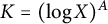 . Let
$m \in [K^{\eta }, 2K^{\eta }]$
. Let
$m \in [K^{\eta }, 2K^{\eta }]$
 be a positive integer. For each prime
$p \in (X,2X]$
be a positive integer. For each prime
$p \in (X,2X]$
 , let
$\mathcal {P}_{\mathbb {H}_p}(m)$
, let
$\mathcal {P}_{\mathbb {H}_p}(m)$
 be defined by (1.4). Then outside an exceptional set of primes
$\mathcal {E} \subseteq (X,2X]$
be defined by (1.4). Then outside an exceptional set of primes
$\mathcal {E} \subseteq (X,2X]$
 depending at most on
$X,\eta ,A$
depending at most on
$X,\eta ,A$
 , and B and satisfying the bound

we have

where
$\mathbb {H}_p$
 and
$H_p$
and
$H_p$
 are defined by (1.3).
Remark 1.1. Theorem 1.1 is essentially sharp in the sense that one cannot establish (1.5) for each individual prime
$ p \in (X,2X] $
 , while working with intervals as small as
$ [1, (\log X)^A] $
, while working with intervals as small as
$ [1, (\log X)^A] $
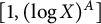 for
$ A> 0 $
for
$ A> 0 $
 . For instance, an application of the Chinese remainder theorem shows that there exist infinitely many primes p for which the least quadratic non-residue is
$\gg \log p$
. For instance, an application of the Chinese remainder theorem shows that there exist infinitely many primes p for which the least quadratic non-residue is
$\gg \log p$
 . Therefore, in such cases,
$\mathbb {H}_p$
. Therefore, in such cases,
$\mathbb {H}_p$
 could be empty. Hence, one must account for an exceptional set of primes, and Theorem 1.1 states that this exceptional set must be thin.
Using Theorem 1.1, we prove the following result regarding the distribution of
$\log \mathcal {P}_{\mathbb {H}_p}(m)$
 . For
$u>1$
. For
$u>1$
 , define the function
$\Psi _u : (0,\infty ) \to \mathbb {R}$
, define the function
$\Psi _u : (0,\infty ) \to \mathbb {R}$
 by
by

where
$\Gamma (t)$
 denotes the Gamma function.
Theorem 1.2 Fix
$\lambda \in \mathbb {R}$
 . Let
$\eta>3 $
. Let
$\eta>3 $
 and
$A>0$
and
$A>0$
 be arbitrary constants. Let
$\{X_j\}$
be arbitrary constants. Let
$\{X_j\}$
 be an increasing sequence of positive real numbers tending to
$\infty $
be an increasing sequence of positive real numbers tending to
$\infty $
 . For each
$X_j$
. For each
$X_j$
 , set
$K_j=(\log X_j)^A$
, set
$K_j=(\log X_j)^A$
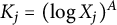 and let
$m_j \in [K_j^{\eta }, 2K_j^{\eta }]$
and let
$m_j \in [K_j^{\eta }, 2K_j^{\eta }]$
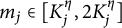 be a positive integer. For each prime
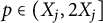
$p \in (X_j,2X_j]$
be a positive integer. For each prime
$p \in (X_j,2X_j]$
 , let
$\mathcal {P}_{\mathbb {H}_p}(m_j)$
, let
$\mathcal {P}_{\mathbb {H}_p}(m_j)$
 be defined by (1.4). Then

where
$\Psi _u(t)$
 is defined by (1.6).
We are also interested in studying partition asymptotics where the parts are small prime quadratic residues and non-residues associated with two distinct primes p and q. Fix an odd prime q and for each prime
$p \in (X,2X]$
 , we define

Let

For
$w \in \mathbb {C}$
 with
$\lvert w \rvert <1$
with
$\lvert w \rvert <1$
 , we consider the generating function

Then
$\mathcal {P}_{\mathbb {H}_{p,q}}(m)$
 represents the number of partitions of a positive integer
$ m $
represents the number of partitions of a positive integer
$ m $
 into parts which lie in
$\mathbb {H}_{p,q}$
into parts which lie in
$\mathbb {H}_{p,q}$
 .
.
In the framework of pretentious number theory, Granville and Soundararajan [Reference Granville and Soundararajan20] introduced a distance function
$ \mathbb {D}(\chi , \psi , y) $
 to quantify how closely two Dirichlet characters
$ \chi $
to quantify how closely two Dirichlet characters
$ \chi $
 and
$ \psi $
and
$ \psi $
 resemble each other up to a positive real number
$ y $
resemble each other up to a positive real number
$ y $
 . More precisely, they define
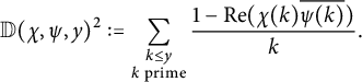
When
$\chi $
 and
$\psi $
and
$\psi $
 are the Legendre symbols modulo p and q, respectively, and
$y=K$
are the Legendre symbols modulo p and q, respectively, and
$y=K$
 ,
$\mathbb {D}(\chi , \psi , K)$
,
$\mathbb {D}(\chi , \psi , K)$
 equals zero if and only if
$( \frac {k}{p})( \frac {k}{q})=1$
equals zero if and only if
$( \frac {k}{p})( \frac {k}{q})=1$
 for each prime
$k \leq K$
for each prime
$k \leq K$
 . In such a scenario, the two characters are indistinguishable up to K, and we have
$a_{k,p,q}=0$
. In such a scenario, the two characters are indistinguishable up to K, and we have
$a_{k,p,q}=0$
 for all
$k \in \mathbb {N}$
for all
$k \in \mathbb {N}$
 . This implies that the set
$\mathbb {H}_{p,q}$
. This implies that the set
$\mathbb {H}_{p,q}$
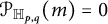
 is empty and
$\mathcal {P}_{\mathbb {H}_{p,q}}(m)=0$
is empty and
$\mathcal {P}_{\mathbb {H}_{p,q}}(m)=0$
 . Our aim below is to provide a context where we are able to show that the two characters are not only distinguishable, but the asymptotic behavior of the partition function
$\mathcal {P}_{\mathbb {H}_{p,q}}(m)$
. Our aim below is to provide a context where we are able to show that the two characters are not only distinguishable, but the asymptotic behavior of the partition function
$\mathcal {P}_{\mathbb {H}_{p,q}}(m)$
 is governed by an underlying Gaussian distribution.
Theorem 1.3 Let
$\eta>3,A>0,$
 and
$B>0$
and
$B>0$
 be arbitrary constants. Fix an odd prime q. Let
$\varepsilon>0$
be arbitrary constants. Fix an odd prime q. Let
$\varepsilon>0$
 . Suppose
$X>0$
. Suppose
$X>0$
 is sufficiently large in terms of
$\eta ,A,B,q$
is sufficiently large in terms of
$\eta ,A,B,q$
 , and
$\varepsilon ,$
, and
$\varepsilon ,$
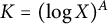
 and
$K=(\log X)^A$
and
$K=(\log X)^A$
 . Let
$m \in [K^{\eta }, 2K^{\eta }]$
. Let
$m \in [K^{\eta }, 2K^{\eta }]$
 be a positive integer. For each prime
$p \in (X,2X]$
be a positive integer. For each prime
$p \in (X,2X]$
 , let
$\mathcal {P}_{\mathbb {H}_{p,q}}(m)$
, let
$\mathcal {P}_{\mathbb {H}_{p,q}}(m)$
 be defined by (1.10). Then outside an exceptional set of primes
$\mathcal {E}\subseteq (X,2X]$
be defined by (1.10). Then outside an exceptional set of primes
$\mathcal {E}\subseteq (X,2X]$
 depending at most on
$X,\eta ,A,B$
depending at most on
$X,\eta ,A,B$
 , and q and satisfying the bound

we have

where
$\mathbb {H}_{p,q}$
 and
$H_{p,q}$
and
$H_{p,q}$
 are defined by (1.9).
We also have the analog of Theorem 1.2 in this context.
Theorem 1.4 Fix
$\lambda \in \mathbb {R}$
 . Let
$\eta>3 $
. Let
$\eta>3 $
 and
$A>0$
and
$A>0$
 be arbitrary constants. Fix an odd prime q. Let
$\{X_j\}$
be arbitrary constants. Fix an odd prime q. Let
$\{X_j\}$
 be an increasing sequence of positive real numbers tending to
$\infty $
be an increasing sequence of positive real numbers tending to
$\infty $
 . For each
$X_j$
. For each
$X_j$
 , set
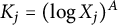
$K_j=(\log X_j)^A$
, set
$K_j=(\log X_j)^A$
 and let
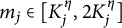
$m_j \in [K_j^{\eta }, 2K_j^{\eta }]$
and let
$m_j \in [K_j^{\eta }, 2K_j^{\eta }]$
 be a positive integer. For each prime
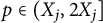
$p \in (X_j,2X_j]$
be a positive integer. For each prime
$p \in (X_j,2X_j]$
 , let
$\mathcal {P}_{\mathbb {H}_{p,q}}(m_j)$
, let
$\mathcal {P}_{\mathbb {H}_{p,q}}(m_j)$
 be defined by (1.10). Then

where
$\Psi _u(t)$
 is defined by (1.6)
Remark 1.2. In contrast to earlier works such as [Reference Basak, Nath and Zaharescu5, Reference Basak, Nath and Zaharescu6], which requires the range of A to satisfy
$A> 1$
 and
$A> 2,$
and
$A> 2,$
 respectively, Theorems 1.1–1.4 allow us to fix any
$A> 0$
respectively, Theorems 1.1–1.4 allow us to fix any
$A> 0$
 for almost all primes, thereby extending well beyond the threshold
$A>2$
for almost all primes, thereby extending well beyond the threshold
$A>2$
 known under GRH. Additionally, we obtain arbitrary log savings on our exceptional set of primes, unlike in [Reference Basak, Nath and Zaharescu5, Reference Basak, Nath and Zaharescu6], where the log saving depended on the choice of A. This is achieved through a combination of high moment estimates, a discretization argument, and an application of the Erdős–Turán inequality.
Remark 1.3. The restriction
$\eta> 3$
 in Theorems 1.1–1.4 reflects the classical threshold
$K = o(m^{\frac {1}{3}})$
in Theorems 1.1–1.4 reflects the classical threshold
$K = o(m^{\frac {1}{3}})$
 that arises in the work of Erdős and Lehner [Reference Erdős and Lehner17]. After completing the proof of Theorem 1.1 in Section 7, we explore the potential for relaxing the range of
$\eta $
that arises in the work of Erdős and Lehner [Reference Erdős and Lehner17]. After completing the proof of Theorem 1.1 in Section 7, we explore the potential for relaxing the range of
$\eta $
 . See Remark 7.1 for more details.
The general framework of Meinardus [Reference Meinardus32] for deriving asymptotics of generating functions represented by infinite products can be readily applied to the study of partitions into parts which lie in arithmetic progressions. For instance, Andrews [Reference Andrews1, Theorem 6.4] shows that

where
$\mathbb {A} = \{ k \in \mathbb {N} : k \equiv b \bmod D \}$
 for some fixed
$D> 0$
for some fixed
$D> 0$
 with
$(b, D) = 1$
with
$(b, D) = 1$
 , and
$C,\kappa $
, and
$C,\kappa $
 are some constants depending only on b and D. Note that the condition
$(b, D) = 1$
are some constants depending only on b and D. Note that the condition
$(b, D) = 1$
 is essential for the validity of the asymptotic formula (1.13), although it seems to be omitted in the statement of [Reference Andrews1, Theorem 6.4]. While the sets
$\mathbb {A}$
is essential for the validity of the asymptotic formula (1.13), although it seems to be omitted in the statement of [Reference Andrews1, Theorem 6.4]. While the sets
$\mathbb {A}$
 considered in our work do not satisfy the analytic assumptions of Meinardus’ theory, we can nevertheless extend Theorems 1.1–1.4 to a broader setting where the parts are small prime quadratic non-residues lying in arithmetic progressions. We present here only the extension of Theorem 1.1. The other extensions follow similarly.
Fix a prime D and let
$b \in (\mathbb {Z}/D\mathbb {Z})^{\times }$
 . For each prime
$p \in (X,2X]$
. For each prime
$p \in (X,2X]$
 , we define

We set

For
$w \in \mathbb {C}$
 with
$\lvert w \rvert <1$
with
$\lvert w \rvert <1$
 , consider the generating function

Theorem 1.5 Let
$\eta>3,A>0,$
 and
$B>0$
and
$B>0$
 be arbitrary constants. Let D be a fixed prime and
$b \in (\mathbb {Z}/D\mathbb {Z})^{\times }$
be arbitrary constants. Let D be a fixed prime and
$b \in (\mathbb {Z}/D\mathbb {Z})^{\times }$
 . Let
$\varepsilon>0$
. Let
$\varepsilon>0$
 . Suppose
$X>0$
. Suppose
$X>0$
 is sufficiently large in terms of
$\eta ,A,B,D$
is sufficiently large in terms of
$\eta ,A,B,D$
 , and
$\varepsilon ,$
, and
$\varepsilon ,$
 and
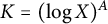
$K=(\log X)^A$
and
$K=(\log X)^A$
 . Let
$m \in [K^{\eta }, 2K^{\eta }]$
. Let
$m \in [K^{\eta }, 2K^{\eta }]$
 be a positive integer. For each prime
$p \in (X, 2X]$
be a positive integer. For each prime
$p \in (X, 2X]$
 , let
$\mathcal {P}_{\widehat {\mathbb {H}}_p}(m)$
, let
$\mathcal {P}_{\widehat {\mathbb {H}}_p}(m)$
 be defined by (1.16). Then outside an exceptional set of primes
$\mathcal {E}\subseteq (X,2X]$
be defined by (1.16). Then outside an exceptional set of primes
$\mathcal {E}\subseteq (X,2X]$
 depending at most on
$X,\eta ,A,B,$
depending at most on
$X,\eta ,A,B,$
 and D and satisfying the bound

we have

where
$\widehat {\mathbb {H}}_p$
 and
$\widehat {H}_p$
and
$\widehat {H}_p$
 are defined by (1.15).
Remark 1.4. With some extra effort, in Theorem 1.5, one can allow D to grow uniformly up to size
$\log \log X$
 . However, for the sake of simplicity, we have refrained from doing so.
Our final result concerns partition asymptotics where the parts are small quadratic residues or non-residues twisted by the Möbius function. For each prime
$p \in (X, 2X]$
 , we define

We define

For
$w \in \mathbb {C}$
 with
$\lvert w \rvert <1$
with
$\lvert w \rvert <1$
 , consider the generating function

Theorem 1.6 Let
$\eta>3,A>0,$
 and
$B>0$
and
$B>0$
 be arbitrary constants. Let
$\varepsilon>0$
be arbitrary constants. Let
$\varepsilon>0$
 . Suppose
$X>0$
. Suppose
$X>0$
 is sufficiently large in terms of
$\eta ,A,B,$
is sufficiently large in terms of
$\eta ,A,B,$
 and
$\varepsilon $
and
$\varepsilon $
 . Let
$m \in [K^{\eta }, 2K^{\eta }]$
. Let
$m \in [K^{\eta }, 2K^{\eta }]$
 be a positive integer. For each prime
$p \in (X, 2X]$
be a positive integer. For each prime
$p \in (X, 2X]$
 , let
$\mathcal {P}_{\mathbb {H}_{p,\mu }}(m)$
, let
$\mathcal {P}_{\mathbb {H}_{p,\mu }}(m)$
 be defined by (1.19). Then outside an exceptional set of primes
$\mathcal {E} \subseteq (X,2X]$
be defined by (1.19). Then outside an exceptional set of primes
$\mathcal {E} \subseteq (X,2X]$
 depending at most on
$X,\eta ,A$
depending at most on
$X,\eta ,A$
 , and B and satisfying the bound

we have

where
$\mathbb {H}_{p,\mu }$
 and
$H_{p, \mu }$
and
$H_{p, \mu }$
 are defined by (1.18).
Remark 1.5. The analog of Theorem 1.2 doesn’t hold for
$\mathcal {P}_{\mathbb {H}_{p,\mu }}(m)$
 . As we shall see in Section 7, the relation (1.12) is closely related to the distribution of short character sums. In the context of Möbius twists, we need to study the distribution of sums of the form
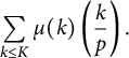
The distribution of these sums is not Gaussian. In fact, the corresponding moments are amplified by extra powers of logs which arise from a connection with moments of a Rademacher random multiplicative function due to Harper–Nikeghbali–Radziwiłł [Reference Harper, Nikeghbali and Radziwiłł23]. For more details, see Lemma 10.1.
The proof of Theorem 1.6 relies on some refined estimates of exponential sums over square-free integers which may be of independent interest. For more details, see Lemmas 10.4 and 10.5.
We conclude this section by briefly mentioning that the shape of the main term in (1.5) differs from that appearing in the classical partition asymptotics such as (1.1). This is due to a distinction in the residue computation which contributes to the main term in each case. For more details, see Remark 5.1.
1.4 Structure of the article
In Section 2, we give a brief overview of the proofs of our main results and highlight how our methods differ from prior works. Standard notations used throughout the article are introduced in Section 3. Section 4 focuses on studying the distribution of short quadratic character sums. The analysis of the main term in the proof of Theorem 1.1 is carried out in Section 5. Section 6 is devoted to bounding the error terms, where we use high-moment estimates for quadratic character sums combined with a discretization argument. The proofs of Theorems 1.1 and 1.2 are completed in Section 7. In Section 8, we address the character twist setting and apply the Erdős–Turán inequality to establish Theorems 1.3 and 1.4. Section 9 contains the proof of Theorem 1.5 which concern the arithmetic progression aspect. Lastly, in Section 10, we prove Theorem 1.6.
2 Outline of the proofs
The proof of Theorem 1.1 begins with the following observation. Suppose we write

where
$w = e^{-\tau }$
 and
$\tau = \sigma +2 \pi i t$
and
$\tau = \sigma +2 \pi i t$
 , with
$\sigma ,t \in \mathbb {R}$
, with
$\sigma ,t \in \mathbb {R}$
 and
$\sigma>0$
and
$\sigma>0$
 . Then, using the orthogonality relation,
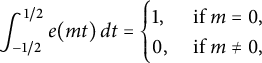
we have

To estimate the integral in (2.2), we need to study the behavior of
$ f_p(\tau ) $
 . Using (2.1), we can write

At this stage, adopting the approach of Meinardus [Reference Meinardus32] (see also [Reference Andrews1, Chapter 6]), we use inverse Mellin transform to derive

where
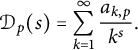
Our first significant difficulty in this analysis arises from the fact that
$ \mathcal {D}_p(s) $
 is a short Dirichlet polynomial in our context, in contrast to the setup of Meinardus, where the Dirichlet series has a pole of order one at
$ s = \alpha $
is a short Dirichlet polynomial in our context, in contrast to the setup of Meinardus, where the Dirichlet series has a pole of order one at
$ s = \alpha $
 for some
$ \alpha>0 $
for some
$ \alpha>0 $
 . Similar assumptions regarding the existence of such a pole are also made in the works of Debruyne–Tenenbaum [Reference Debruyne and Tenenbaum14] and Bridges–Brindle–Bringmann–Franke [Reference Bridges, Brindle, Bringmann and Franke9]. Since our corresponding Dirichlet polynomial
$ \mathcal {D}_p(s) $
. Similar assumptions regarding the existence of such a pole are also made in the works of Debruyne–Tenenbaum [Reference Debruyne and Tenenbaum14] and Bridges–Brindle–Bringmann–Franke [Reference Bridges, Brindle, Bringmann and Franke9]. Since our corresponding Dirichlet polynomial
$ \mathcal {D}_p(s) $
 has no poles, the methods developed in [Reference Bridges, Brindle, Bringmann and Franke9, Reference Debruyne and Tenenbaum14, Reference Meinardus32] are not applicable to our setting. To this end, we directly work with
$\mathcal {D}_p(s)$
has no poles, the methods developed in [Reference Bridges, Brindle, Bringmann and Franke9, Reference Debruyne and Tenenbaum14, Reference Meinardus32] are not applicable to our setting. To this end, we directly work with
$\mathcal {D}_p(s)$
 , and a standard contour integration argument reveals that the main term in the asymptotic expansion of
$\mathcal {P}_{\mathbb {H}_p}(m)$
, and a standard contour integration argument reveals that the main term in the asymptotic expansion of
$\mathcal {P}_{\mathbb {H}_p}(m)$
 arises from a double pole at
$s=0$
arises from a double pole at
$s=0$
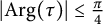
 in the integrand of (2.3) when
$ \lvert \operatorname {Arg}(\tau ) \rvert \leq \tfrac {\pi }{4} $
in the integrand of (2.3) when
$ \lvert \operatorname {Arg}(\tau ) \rvert \leq \tfrac {\pi }{4} $
 .
.
The analysis of the error term, corresponding to the range
$ \tfrac {\pi }{4} < \lvert \operatorname {Arg}(\tau ) \rvert \leq \tfrac {\pi }{2} $
 , is more intricate and occupies the rest of the proof. As part of this, we aim to derive upper bounds for the expression

These bounds depend crucially on the cardinality of
$\mathbb {H}_p$
 , denoted by
$H_p$
, denoted by
$H_p$
 . Heuristically, one expects
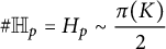
for each individual prime p, based on the natural assumption that on average, the “probability” of a randomly chosen integer
$ k \in [1, p-1] $
 being a quadratic non-residue is
$ \frac {1}{2} $
being a quadratic non-residue is
$ \frac {1}{2} $
 . Unfortunately, establishing (2.5) for every individual prime
$ p $
. Unfortunately, establishing (2.5) for every individual prime
$ p $
 , particularly in intervals as small as
$ [1, (\log X)^A] $
, particularly in intervals as small as
$ [1, (\log X)^A] $
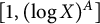 for any
$ A> 0 $
for any
$ A> 0 $
 , remains beyond current knowledge. As discussed in Section 1, even assuming GRH, it is only known that
$H_p \geq 1 $
, remains beyond current knowledge. As discussed in Section 1, even assuming GRH, it is only known that
$H_p \geq 1 $
 if we allow
$A\geq 2$
if we allow
$A\geq 2$
 . Moreover, as pointed out in Remark 1.1, it is possible to have
$H_p=0$
. Moreover, as pointed out in Remark 1.1, it is possible to have
$H_p=0$
 for smaller values of A, in which case we are unable to obtain a nontrivial upper bound for (2.4).
This motivates the idea of bounding (2.4) for almost all primes, which leads to our second significant challenge: estimating the right-hand side of (2.4) on average over primes. Roughly speaking, this task reduces to bounding weighted exponential sums of the form
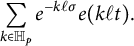
At this stage, there are two different methods to approach this problem. The first involves detecting the condition
$\mathbb {1}_{k \in \mathbb {H}_p}$
 in (2.6) via quadratic characters. This leads to two distinct exponential sums: the first is a classical exponential sum over primes, which can be bounded using Vinogradov’s estimates; the second is twisted by quadratic characters and is handled by bounding its high moments. A key technical step in this approach is to carefully discretize the continuous variable t. This enables us to derive the required upper bounds for (2.4) for all but a thin exceptional set of primes. A detailed treatment of this method is presented in Section 6. The second method focuses on those primes p for which
$H_p$
in (2.6) via quadratic characters. This leads to two distinct exponential sums: the first is a classical exponential sum over primes, which can be bounded using Vinogradov’s estimates; the second is twisted by quadratic characters and is handled by bounding its high moments. A key technical step in this approach is to carefully discretize the continuous variable t. This enables us to derive the required upper bounds for (2.4) for all but a thin exceptional set of primes. A detailed treatment of this method is presented in Section 6. The second method focuses on those primes p for which
$H_p$
 is sufficiently large. In this setting, we use the equidistribution of the sequence
$kt$
is sufficiently large. In this setting, we use the equidistribution of the sequence
$kt$
 modulo
$1$
modulo
$1$
 as k varies over
$\mathbb {H}_p$
as k varies over
$\mathbb {H}_p$
 . This approach relies on the Erdős–Turán inequality to quantify the equidistribution, combined with the Siegel–Walfisz theorem to control the distribution of primes in arithmetic progressions. A full exposition of this method appears in Section 8, in the proof of Theorem 1.3. An application of the saddle point method with the choice
$\sigma = \sigma _p = H_p/m$
. This approach relies on the Erdős–Turán inequality to quantify the equidistribution, combined with the Siegel–Walfisz theorem to control the distribution of primes in arithmetic progressions. A full exposition of this method appears in Section 8, in the proof of Theorem 1.3. An application of the saddle point method with the choice
$\sigma = \sigma _p = H_p/m$
 , together with other analytic arguments, completes the proof of Theorem 1.1 in Section 7.
To obtain our distribution result, that is, Theorem 1.2, we study moments of short character sums. These moments are determined separately through a mix of combinatorial arguments, quadratic reciprocity, and distribution of primes in arithmetic progressions. Then we combine our moment estimates and the asymptotic estimate (1.5) from Theorem 1.1 to prove Theorem 1.2. The proof of Theorem 1.4 follows similar arguments.
Our final challenge is to extend the proofs to more general settings that incorporate additional arithmetic constraints. In Theorem 1.5, where the variable k is restricted to lie in arithmetic progressions modulo D, we require a more careful analysis of (2.6). In particular, we require a variant of Vinogradov’s bounds that makes the dependence on the modulus D explicit. This is carried out in Section 9, in Lemmas 9.3 and 9.4. In the Möbius case, as discussed in Remark 1.5, the limiting distribution is no longer Gaussian. Instead, the moments are amplified by powers of logs (see Lemma 10.1). We also need some refined estimates for exponential sums over square-free integers, in particular, Lemmas 10.4 and 10.5, which are essential for bounding the analogous version of (2.6) that appears in this context.
3 General notations
We employ some standard notation that will be used throughout the article:
-
• Throughout the article, the expressions $f(X)=O(g(X))$
 ,
$f(X) \ll g(X)$
, and
$g(X) \gg f(X)$
are equivalent to the statement that
$|f(X)| \leq C|g(X)|$
for all sufficiently large X, where
$C>0$
is an absolute constant. A subscript of the form
$\ll _{\alpha }$
means the implied constant may depend on the parameter
$\alpha $
. Dependence on several parameters is indicated in an analogous manner, as in
$\ll _{\alpha , \lambda }$
.
,
$f(X) \ll g(X)$
, and
$g(X) \gg f(X)$
are equivalent to the statement that
$|f(X)| \leq C|g(X)|$
for all sufficiently large X, where
$C>0$
is an absolute constant. A subscript of the form
$\ll _{\alpha }$
means the implied constant may depend on the parameter
$\alpha $
. Dependence on several parameters is indicated in an analogous manner, as in
$\ll _{\alpha , \lambda }$
. -
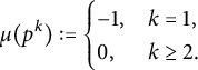
• Let $\mu $
denote the Möbius function, which is a multiplicative function defined as follows: for each prime p, $$\begin{align*}\mu(p^k) := \begin{cases} -1, & k=1, \\ 0, & k \geq 2. \end{cases}\end{align*}$$
-
• For a prime p, the Legendre symbol $(\frac {\cdot }{p})$
is defined by $$\begin{align*}\bigg(\frac{n}{p}\bigg):= \begin{cases} 1, & \text{if } n \text{ is a quadratic residue modulo p},\\ 0, &\text{if } p|n,\\ -1, & \text{if } n \text{ is a quadratic non-residue modulo p}. \end{cases} \end{align*}$$
For any integer k and any positive odd integer n, the Jacobi symbol $\left (\frac {k}{n}\right )$
is defined as the product of the Legendre symbols corresponding to the prime factors of n. We have $$ \begin{align*} \bigg(\frac{k}{n}\bigg):=\bigg(\frac{k}{p_1}\bigg)^{\alpha_1}\bigg(\frac{k}{p_2}\bigg)^{\alpha_2} \cdots\bigg(\frac{k}{p_k}\bigg)^{\alpha_k}, \end{align*} $$where $ n=p_1^{\alpha _1} p_2^{\alpha _2} \ldots p_k^{\alpha _k} $
is the prime factorization of n.
-
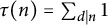
• For $n \in \mathbb {N}$
,
$\tau (n)$
denotes the divisor function given by
$\tau (n) = \sum _{d \mid n} 1$
. -
• For $n \in \mathbb {N}$
,
$\varphi (n)$
denotes the Euler totient function given by
$\varphi (n) = \ \sum _{1 \leq m \leq n, (m,n)=1} 1$
. -
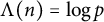
• For $n \in \mathbb {N}$
,
$\Lambda (n)$
denotes the von Mangoldt function given by
$\Lambda (n) = \log p$
if
$n=p^k$
for some prime p and
$k \in \mathbb {N}$
, and zero otherwise. -
• For $n \in \mathbb {N}$
,
$[n]$
denotes the interval
$\{1,\dots ,n\}$
. -
• We write $e(t) = e^{2\pi i t}$
. -
• For any set $\mathcal {A}$
,
$\#\mathcal {A}$
denotes the cardinality of the set
$\mathcal {A}$
. -
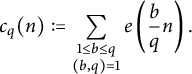
• For $q,n \in \mathbb {N}$
, we define the Ramanujan sum $$\begin{align*}c_q(n) := \sum_{\substack{1 \leq b \leq q \\ (b,q)=1}}e\left ( \frac{b}{q}n \right). \end{align*}$$
We shall use the bound $\lvert c_q(n) \rvert \leq (n,q).$
-
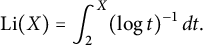
• For $X \geq 2$
,
$\pi (X)$
denotes the number of primes up to X,
$\pi (X;q,a)$
denotes the number of primes congruent to
$a \bmod q$
, and the function Li
$(X)$
is the logarithmic integral defined by $$\begin{align*}\text{Li}(X) = \int_{2}^{X} (\log t)^{-1} \, dt. \end{align*}$$
-
• Throughout the article, the symbols $c_0, c_1, c_2,\dots ,C_0,C_1,C_2 \dots $
denote absolute constants. -
• The notation $ k = \square $
indicates that
$ k $
is a perfect square, while
$ k \neq \square $
signifies that
$ k $
is not a perfect square. -
• We denote by $\varepsilon $
an arbitrarily small positive quantity that may vary from one line to the next, or even within the same line. Thus, we may write
$X^{2\varepsilon } \leq X^{\varepsilon }$
with no reservations. -
• The notation $\sum_{1 \leq n \leq X}^{\mathfrak{b}}$
denotes the sum running over n square-free in
$[1,X]$
.


























4 Distribution of short quadratic character sums
Suppose
$ X> 0 $
 is sufficiently large, and let
$ A> 0 $
is sufficiently large, and let
$ A> 0 $
 be an arbitrary constant. Set
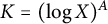
$K=(\log X)^A$
be an arbitrary constant. Set
$K=(\log X)^A$
 . For each prime
$ p $
. For each prime
$ p $
 in the interval
$ (X, 2X] $
in the interval
$ (X, 2X] $
 , define the sum
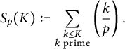
Our goal in this section is to study the distribution of
$S_{p}(K)$
 . This will be useful in the proof of Theorem 1.2 in Section 7. We begin with an auxiliary lemma that addresses cancellations in sums involving quadratic characters.
Lemma 4.1 Let
$ A> 0 $
 and
$B>0$
and
$B>0$
 be arbitrary constants. Suppose
$ X> 0 $
be arbitrary constants. Suppose
$ X> 0 $
 is sufficiently large in terms of A and B. Let
$ k \in \mathbb {N} $
is sufficiently large in terms of A and B. Let
$ k \in \mathbb {N} $
 satisfy
$ 2 \leq k \leq (\log X)^A $
satisfy
$ 2 \leq k \leq (\log X)^A $
 , with
$ k $
, with
$ k $
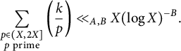
 not a perfect square. Then we have
Proof Our tool here is the Siegel–Walfisz theorem [Reference Iwaniec and Kowalski26, Equation (5.77)]. Let
$ k_0 $
 be the square-free part of
$ k $
be the square-free part of
$ k $
 . Then
$ k_0 \geq 2 $
. Then
$ k_0 \geq 2 $
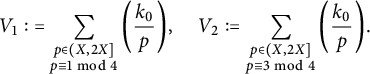
 . By the multiplicativity of Legendre symbols, we write

where
We consider the following cases.
Case 1:
$k_0$
 odd. Using quadratic reciprocity, we can express
$ V_1 $
odd. Using quadratic reciprocity, we can express
$ V_1 $
 as
as

Here, we have noted that
$ (p, k_0) = 1 $
 and used the Chinese remainder theorem to consolidate the congruence conditions. By the Siegel–Walfisz theorem, for any
$B>0$
and used the Chinese remainder theorem to consolidate the congruence conditions. By the Siegel–Walfisz theorem, for any
$B>0$
 , we find that

The sum over
$ a $
 is a complete character sum, which is equal to zero. Hence, by suitably adjusting the parameter B to absorb the factor
$\varphi (k_0)$
is a complete character sum, which is equal to zero. Hence, by suitably adjusting the parameter B to absorb the factor
$\varphi (k_0)$
 , we have
$V_1 \ll _{A,B} X(\log X)^{-B}$
, we have
$V_1 \ll _{A,B} X(\log X)^{-B}$
 for any
$B>0$
for any
$B>0$
 .
.
Case 2:
$k_0$
 even. Since
$k_0$
even. Since
$k_0$
 is square-free, we must have
$k_0=2k_0'$
is square-free, we must have
$k_0=2k_0'$
 with
$k_0'$
with
$k_0'$
 odd. We again apply quadratic reciprocity to write
$ V_1 $
odd. We again apply quadratic reciprocity to write
$ V_1 $
 as
as
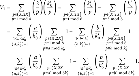
Similar to the previous case, using the Siegel–Walfisz theorem, for any
$B>0$
 ,
$V_1 \ll _{A,B} X(\log X)^{-B}$
,
$V_1 \ll _{A,B} X(\log X)^{-B}$
 .
.
The same case-by-case treatment applies to
$V_2$
 as well, and the desired conclusion follows.
Our next lemma shows that the moments of
$ S_{p}(K) $
 exhibit properties of a Gaussian distribution.
Lemma 4.2 Let
$ A> 0 $
 and
$B>0$
and
$B>0$
 be arbitrary constants. Suppose
$ X> 0 $
be arbitrary constants. Suppose
$ X> 0 $
 is sufficiently large in terms of A and B, and set
$K=(\log X)^A$
is sufficiently large in terms of A and B, and set
$K=(\log X)^A$
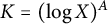 . For each prime
$ p \in (X, 2X] $
. For each prime
$ p \in (X, 2X] $
 , let
$ S_{p}(K) $
, let
$ S_{p}(K) $
 be defined by (4.1). Fix
$ r \in \mathbb {N} $
be defined by (4.1). Fix
$ r \in \mathbb {N} $
 . Then we have
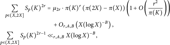
where
$ \mu _{2r} = (2r-1)(2r-3) \dots 3 \cdot 1 $
 is the
$ 2r $
is the
$ 2r $
 -th moment of a standard Gaussian.
Proof Consider first the case when the exponent is even. Expanding the power, we write

where
$ N_{r,K} $
 denotes the number of tuples
$ (k_1, \dots ,k_{2r}) $
denotes the number of tuples
$ (k_1, \dots ,k_{2r}) $
 such that
$ 2 \leq k_i \leq K $
such that
$ 2 \leq k_i \leq K $
 ,
$ k_i $
,
$ k_i $
 is prime, and the product
$ k_1 \ldots k_{2r} $
is prime, and the product
$ k_1 \ldots k_{2r} $
 is a perfect square. For such tuples, there are at most r distinct entries, and each must occur an even number of times. The number of ways to choose exactly r distinct primes from
$\{2, \ldots , K\}$
is a perfect square. For such tuples, there are at most r distinct entries, and each must occur an even number of times. The number of ways to choose exactly r distinct primes from
$\{2, \ldots , K\}$
 is
$\left (\frac {1}{r!}\right ) \pi (K)(\pi (K)-1) \dots (\pi (K)-r+1)$
is
$\left (\frac {1}{r!}\right ) \pi (K)(\pi (K)-1) \dots (\pi (K)-r+1)$
 , and the number of ways to arrange these as r pairs is
$\frac {(2 r)!}{2^r}=r!(2 r-1) \cdot (2 r-3) \dots 3 \cdot 1$
, and the number of ways to arrange these as r pairs is
$\frac {(2 r)!}{2^r}=r!(2 r-1) \cdot (2 r-3) \dots 3 \cdot 1$
 . Hence, we obtain the inequality

Also, the number of ways of choosing at most r distinct primes from
$2, \ldots , K$
 is less than or equal to
$\pi (K)^{r}$
is less than or equal to
$\pi (K)^{r}$
 . When these have been chosen, the number of different ways of arranging them in
$2 r$
. When these have been chosen, the number of different ways of arranging them in
$2 r$
 places (each occurring an even number of times) is at most
$(2 r-1)\cdot (2 r-3) \dots 5 \cdot 3 \cdot 1$
places (each occurring an even number of times) is at most
$(2 r-1)\cdot (2 r-3) \dots 5 \cdot 3 \cdot 1$
 . Therefore, we get

Using the crude estimate,
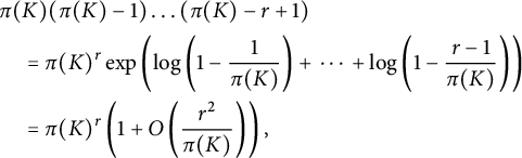
and combining (4.3) and (4.4), we derive

Now, we bound the contribution from the cases where the product
$ k_1 \ldots k_{2r} $
 is not a perfect square. By Lemma 4.1, for any
$B>0$
is not a perfect square. By Lemma 4.1, for any
$B>0$
 ,
,

Substituting (4.5) and (4.6) in (4.2), we obtain

This completes the proof for the even exponent case. When the exponent is odd, the proof is similar except that the product
$k_1\ldots k_{2r-1}$
 is never a perfect square.
Lemma 4.2 furnishes the following distribution result.
Lemma 4.3 Let
$ A> 0 $
 be an arbitrary constant. Then for any
$\lambda \in \mathbb {R}$
be an arbitrary constant. Then for any
$\lambda \in \mathbb {R}$
 ,
,

Proof By our definition of
$S_p(K)$
 , the condition
$H_p \leq \tfrac {1}{2}( \pi (K)+\lambda \cdot \pi (K)^{\frac {1}{2}} )$
, the condition
$H_p \leq \tfrac {1}{2}( \pi (K)+\lambda \cdot \pi (K)^{\frac {1}{2}} )$
 is equivalent to
$S_{p}(K) \geq - \lambda \cdot \pi (K)^{\frac {1}{2}}$
is equivalent to
$S_{p}(K) \geq - \lambda \cdot \pi (K)^{\frac {1}{2}}$
 . By Lemma 4.2, for every fixed positive integer j, we have

where

The proof now follows using the moment method and an application of the Berry–Esseen theorem. See [Reference Basak, Nath and Zaharescu5, Reference Davenport and Erdös13] for such applications.
5 Theorem 1.1: Main term analysis
Let the notations be as in Sections 1 and 4. For the reader’s convenience, we revisit some definitions from Section 1. For each prime
$p \in (X, 2X]$
 , we set

We defined

Let
$\tau = \sigma + 2 \pi i t$
 , where
$\sigma , t \in \mathbb {R}$
, where
$\sigma , t \in \mathbb {R}$
 with
$\sigma> 0$
with
$\sigma> 0$
 . Recall the generating function

where
$w = e^{-\tau }$
 . Our goal here is to study the behavior of
$\log f_p(\tau )$
. Our goal here is to study the behavior of
$\log f_p(\tau )$
 . The behavior of
$\log f_p(\tau )$
. The behavior of
$\log f_p(\tau )$
 is influenced by the argument of
$\tau $
is influenced by the argument of
$\tau $
 . Specifically, the cases
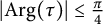
$\lvert \operatorname {Arg}(\tau ) \rvert \leq \frac {\pi }{4}$
. Specifically, the cases
$\lvert \operatorname {Arg}(\tau ) \rvert \leq \frac {\pi }{4}$
 and
$\frac {\pi }{4} < \lvert \operatorname {Arg}(\tau ) \rvert \leq \frac {\pi }{2}$
and
$\frac {\pi }{4} < \lvert \operatorname {Arg}(\tau ) \rvert \leq \frac {\pi }{2}$
 will require separate analysis. In this section, we focus on the case where
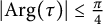
$\lvert \operatorname {Arg}(\tau ) \rvert \leq \frac {\pi }{4}$
will require separate analysis. In this section, we focus on the case where
$\lvert \operatorname {Arg}(\tau ) \rvert \leq \frac {\pi }{4}$
 , as this range contributes to the main term in our partition asymptotic formula (1.5) in Theorem 1.1.
Lemma 5.1 Let
$c\in (0,1)$
 and
$A>0$
and
$A>0$
 be arbitrary constants. Let
$\tau = \sigma + 2\pi i t$
be arbitrary constants. Let
$\tau = \sigma + 2\pi i t$
 , where
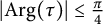
$\left | \operatorname {Arg}(\tau ) \right | \leq \frac {\pi }{4}$
, where
$\left | \operatorname {Arg}(\tau ) \right | \leq \frac {\pi }{4}$
 and
$\sigma , t \in \mathbb {R}$
and
$\sigma , t \in \mathbb {R}$
 satisfy
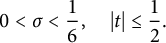
Suppose
$X>0$
 is sufficiently large in terms of c and A, and set
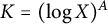
$K=(\log X)^A$
is sufficiently large in terms of c and A, and set
$K=(\log X)^A$
 . For each prime
$p \in (X, 2X]$
. For each prime
$p \in (X, 2X]$
 , let
$f_p(\tau )$
, let
$f_p(\tau )$
 be defined by (5.2). Then uniformly for
$\lvert t \rvert \leq \frac {1}{2} $
be defined by (5.2). Then uniformly for
$\lvert t \rvert \leq \frac {1}{2} $
 ,
,

Proof We begin by expressing
$\log f_p(\tau )$
 as
as

For
$\operatorname {Re}(\tau ) = \sigma>0$
 , using the inverse Mellin transform, we find that

Substituting this into (5.4), we obtain

where
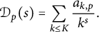
Our goal now is to estimate the integral on the right-hand side of (5.5). The path of integration in (5.5) is taken along the vertical line
$\operatorname {Re}(s) = 2$
 . We modify the path for
$|t| \leq T$
. We modify the path for
$|t| \leq T$
 by moving it leftward and replacing it with a rectangular contour. This new contour connects the points
$2 \pm i T$
by moving it leftward and replacing it with a rectangular contour. This new contour connects the points
$2 \pm i T$
 and
$-c \pm i T$
and
$-c \pm i T$
 , where
$c\in (0,1)$
, where
$c\in (0,1)$
 . The resulting path of integration L consists of the segments
$L = \bigcup _{i=1}^5 L_i$
. The resulting path of integration L consists of the segments
$L = \bigcup _{i=1}^5 L_i$
 , defined as follows:
$L_1 : (2 - i\infty , 2 - iT], L_2 : [2 - iT, -c - iT], L_3 : [-c - iT, -c + iT], L_4 : [-c + iT, 2 + iT]$
, defined as follows:
$L_1 : (2 - i\infty , 2 - iT], L_2 : [2 - iT, -c - iT], L_3 : [-c - iT, -c + iT], L_4 : [-c + iT, 2 + iT]$
 , and
$L_5 : [2 + iT, 2 + i\infty )$
, and
$L_5 : [2 + iT, 2 + i\infty )$
 . Using this modified path, the Cauchy residue theorem gives
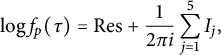
where
$\text {Res}$
 accounts for the residues of the integrand’s singularities enclosed by the original and modified paths, and
$I_{j}$
accounts for the residues of the integrand’s singularities enclosed by the original and modified paths, and
$I_{j}$
 represents the integrals along the respective segments
$L_j$
represents the integrals along the respective segments
$L_j$
 . The integrand in (5.5) has a double pole at
$s=0$
. The integrand in (5.5) has a double pole at
$s=0$
 . Computing the residue, we derive

To estimate the integrals
$I_{j}$
 , we rely on the following bounds:



for some constant
$C>0$
 depending only on c. Since
$\lvert \operatorname {Arg}(\tau )\rvert \leq \frac {\pi }{4}$
depending only on c. Since
$\lvert \operatorname {Arg}(\tau )\rvert \leq \frac {\pi }{4}$
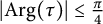 , the absolute value of
$\tau ^{-s}$
, the absolute value of
$\tau ^{-s}$
 can be bounded as follows:

Consider first the integral
$I_5$
 . In our range of integration, we have
$\zeta (s+1), \mathcal {D}_p(s) \ll 1$
. In our range of integration, we have
$\zeta (s+1), \mathcal {D}_p(s) \ll 1$
 . Therefore, using the bounds (5.8), (5.9), and (5.11), we find that

An analogous argument holds for
$I_{1}$
 . So, we obtain

Now, we consider the horizontal integrals
$I_2$
 and
$I_4$
and
$I_4$
 . Using (5.8)–(5.11), we have
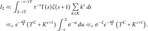
A similar bound holds for
$I_4$
 . Therefore, we obtain

Finally, it remains to estimate the vertical integral
$I_3$
 . To this end, using (5.8)–(5.11), we have
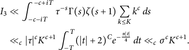
Putting together (5.6), (5.7), (5.12), (5.14), and (5.15), and letting
$T \to \infty $
 , we arrive at

Noting that
$\mathcal {D}_p'(0)= -\log ( \prod _{k \in \mathbb {H}_p} k )$
 and
$\mathcal {D}_p(0) = H_p$
and
$\mathcal {D}_p(0) = H_p$
 , we complete the proof.
Remark 5.1. The shape of the main term in (1.5) differs from that appearing in the classical partition asymptotics, such as (1.1). This distinction arises due to the analytic structure of the integrand in (5.5): in our setting, the integrand has a double pole at
$s=0$
 which contributes to the main term, whereas in the case of (1.1), the integrand is
$\tau ^{-s}\Gamma (s)\zeta (s+1)\zeta (s)$
which contributes to the main term, whereas in the case of (1.1), the integrand is
$\tau ^{-s}\Gamma (s)\zeta (s+1)\zeta (s)$
 which possesses a simple pole at
$s=1$
which possesses a simple pole at
$s=1$
 , and the residue from this simple pole gives rise to the main term.
6 Theorem 1.1: Error term analysis
In this section, we address the behavior of
$ \log f_p(\tau ) $
 when
$ \tfrac {\pi }{4} < \lvert \operatorname {Arg}(\tau ) \rvert \leq \tfrac {\pi }{2} $
when
$ \tfrac {\pi }{4} < \lvert \operatorname {Arg}(\tau ) \rvert \leq \tfrac {\pi }{2} $
 . Our primary focus is on establishing upper bounds, as these values of
$ \tau $
. Our primary focus is on establishing upper bounds, as these values of
$ \tau $
 contribute only to the error term in Theorem 1.1. Let the notations be as in Sections 1, 4, and 5. Since the parameter
$\sigma $
contribute only to the error term in Theorem 1.1. Let the notations be as in Sections 1, 4, and 5. Since the parameter
$\sigma $
 will later depend on the prime
$ p $
will later depend on the prime
$ p $
 in Section 7, it is essential to make this dependence explicit here. For each prime
$ p \in (X, 2X] $
in Section 7, it is essential to make this dependence explicit here. For each prime
$ p \in (X, 2X] $
 , we set

where
$ H_p $
 is given by (5.1). Recall from Section 1 that
$ m \in [K^{\eta },2K^{\eta }] $
is given by (5.1). Recall from Section 1 that
$ m \in [K^{\eta },2K^{\eta }] $
 for some
$ \eta> 3 $
for some
$ \eta> 3 $
 , where
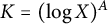
$K=(\log X)^A$
, where
$K=(\log X)^A$
 . In fact, the results in this section will hold in the wider range
$\eta>2$
. In fact, the results in this section will hold in the wider range
$\eta>2$
 .
.
Lemma 6.1 Let
$\eta>2,A>0$
 , and
$B>0$
, and
$B>0$
 be arbitrary constants. Suppose
$X>0$
be arbitrary constants. Suppose
$X>0$
 is sufficiently large in terms of
$\eta ,A$
is sufficiently large in terms of
$\eta ,A$
 , and B, and set
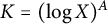
$K=(\log X)^A$
, and B, and set
$K=(\log X)^A$
 . For each prime
$p \in (X, 2X]$
. For each prime
$p \in (X, 2X]$
 , let
$f_p(\tau )$
, let
$f_p(\tau )$
 be defined by (5.2) and
$\sigma _p$
be defined by (5.2) and
$\sigma _p$
 be as in (6.1). There exists a constant
$C_0>0$
be as in (6.1). There exists a constant
$C_0>0$
 such that outside an exceptional set of primes
$\mathcal {F} \subseteq (X, 2X]$
such that outside an exceptional set of primes
$\mathcal {F} \subseteq (X, 2X]$
 , which depends at most on
$ X, \eta $
, which depends at most on
$ X, \eta $
 , and
$A $
, and
$A $
 , and satisfies

we have the uniform bounds
$H_p \geq \frac {\pi (K)}{3}$
 and
and

Proof Define

If
$H_p < \tfrac {\pi (K)}{3}$
 , then
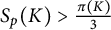
$S_{p}(K)> \tfrac {\pi (K)}{3}$
, then
$S_{p}(K)> \tfrac {\pi (K)}{3}$
 , where
$S_{p}(K)$
, where
$S_{p}(K)$
 is as in (4.1). Then by Lemma 4.2, for any
$r \in \mathbb {N}$
is as in (4.1). Then by Lemma 4.2, for any
$r \in \mathbb {N}$
 ,
,

By choosing
$ r $
 sufficiently large in terms of
$ \eta $
sufficiently large in terms of
$ \eta $
 ,
$ A $
,
$ A $
 , and
$ B $
, and
$ B $
 , it follows that
$\# \mathcal {F} \ll _{\eta , A, B} X (\log X)^{-B}$
, it follows that
$\# \mathcal {F} \ll _{\eta , A, B} X (\log X)^{-B}$
 . Therefore, for all primes
$ p \in (X, 2X] \setminus \mathcal {F} $
. Therefore, for all primes
$ p \in (X, 2X] \setminus \mathcal {F} $
 , we have the uniform bound
$H_p \geq \tfrac {\pi (K)}{3}$
, we have the uniform bound
$H_p \geq \tfrac {\pi (K)}{3}$
 which implies that
$\sigma _p \geq \tfrac {\pi (K)}{3m}$
which implies that
$\sigma _p \geq \tfrac {\pi (K)}{3m}$
 . Throughout the rest of the proof, we will restrict ourselves to working with primes from the set
$(X, 2X] \setminus \mathcal {F}$
. Throughout the rest of the proof, we will restrict ourselves to working with primes from the set
$(X, 2X] \setminus \mathcal {F}$
 . We consider two cases depending on the range of t.
Case 1:
$(\log K)^{-\frac {1}{2}} \leq \lvert 2\pi K t \rvert \leq \sqrt {10}$
 . By (5.4) and nonnegativity,
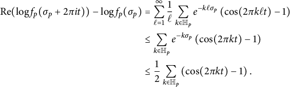
By the prime number theorem and partial summation, for
$p \in (X,2X]\setminus \mathcal {F}$
 ,
,
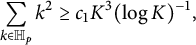
for some constant
$c_1>0$
 . Therefore, by Taylor expansion, the right-hand side of (6.3) is

for some constant
$c_2>0$
 .
.
Case 2:
$ K \sigma _p \leq \lvert 2\pi K t \rvert < (\log K)^{-\frac {1}{2}}$
 . In this range, (6.3) is no longer efficient. Indeed, when t is small, the terms with
$\ell \asymp \sigma _p^{-1}$
. In this range, (6.3) is no longer efficient. Indeed, when t is small, the terms with
$\ell \asymp \sigma _p^{-1}$
 can significantly contribute to the left-hand side of (6.3). Rather than relying on (6.3), we work directly with (5.4). We write

By Taylor expansion, we have

which implies that

Another application of the Taylor expansion shows that

Substituting (6.5) and (6.6) in (6.4), we see that the right-hand side of (6.4) is

It follows that in this case,

for some constant
$c_3>0$
 .
.
Combining Cases 1 and 2 and choosing
$C_0 = \min \{c_2,c_3 \}$
 , we arrive at our desired conclusion.
We now address the range
$ \lvert 2 \pi Kt \rvert> \sqrt {10}$
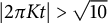 . Here, we will use a high moment approach followed by a discretization argument. Later, in Section 8, we will prove an analogous result for the character twist case using the Erdős–Turán inequality. We first establish some estimates on certain weighted exponential sums over primes.
Lemma 6.2 Let
$\eta>2$
 and
$A>0$
and
$A>0$
 be arbitrary constants. Suppose
$X>0$
be arbitrary constants. Suppose
$X>0$
 is sufficiently large in terms of
$\eta $
is sufficiently large in terms of
$\eta $
 and A, and set
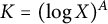
$K=(\log X)^A$
and A, and set
$K=(\log X)^A$
 . For each prime
$p \in (X, 2X]$
. For each prime
$p \in (X, 2X]$
 , let
$\sigma _p$
, let
$\sigma _p$
 be defined as in (6.1). Then there exists a constant
$C_1>0$
be defined as in (6.1). Then there exists a constant
$C_1>0$
 such that the following uniform bound holds:

Proof For
$X>0$
 sufficiently large, uniformly for all
$p \in (X,2X]$
sufficiently large, uniformly for all
$p \in (X,2X]$
 , we have

To handle the right-hand side of (6.8), we will use Vinogradov’s bound on exponential sums over primes [Reference Davenport12, Chapter 25]. If
$\lvert t-u/v\rvert \leq 1/v^2$
 with
$(u,v)=1$
with
$(u,v)=1$
 , then

Let
$K_1 = K(\log K)^{-10}.$
 By Dirichlet’s theorem on Diophantine approximation, for
$t \in \mathbb {R}$
By Dirichlet’s theorem on Diophantine approximation, for
$t \in \mathbb {R}$
 , there exists a reduced fraction
$u/v$
, there exists a reduced fraction
$u/v$
 with
$1 \leq v \leq K_1$
with
$1 \leq v \leq K_1$
 such that
$\lvert t-u/v \rvert \leq 1/(vK_1) \leq 1/v^2$
such that
$\lvert t-u/v \rvert \leq 1/(vK_1) \leq 1/v^2$
 . If
$v \geq (\log K)^{10}$
. If
$v \geq (\log K)^{10}$
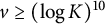 , then by (6.9) and partial summation, we have
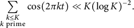
When
$3 \leq v \leq (\log K)^{10}$
 , then writing
$t=u/v+\beta $
, then writing
$t=u/v+\beta $
 , we have, for any
$B>0$
, we have, for any
$B>0$
 (see [Reference Davenport12, Chapter 26]),

where
$T(\beta ) = \sum _{k \leq K} e(k \beta )$
 . We trivially bound
$T(\beta )$
. We trivially bound
$T(\beta )$
 and use partial summation to obtain
Finally, we are left with
$v=1,2$
 . For
$v=1$
. For
$v=1$
 , since
$\sqrt {10}/(2\pi K) < \lvert \beta \rvert \leq K_1^{-1}$
, since
$\sqrt {10}/(2\pi K) < \lvert \beta \rvert \leq K_1^{-1}$
 , instead of trivially bounding
$T(\beta )$
, instead of trivially bounding
$T(\beta )$
 , we use the sharper bound
$\lvert T(\beta ) \rvert \leq \lvert \sin (\pi \beta ) \rvert ^{-1} \leq \pi K/\sqrt {10}.$
, we use the sharper bound
$\lvert T(\beta ) \rvert \leq \lvert \sin (\pi \beta ) \rvert ^{-1} \leq \pi K/\sqrt {10}.$
 When
$v=2$
When
$v=2$
 , we have
$\lvert \beta \rvert \leq 1/(2K_1)$
, we have
$\lvert \beta \rvert \leq 1/(2K_1)$
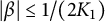 , and therefore, the same approach as in the case
$v=1$
, and therefore, the same approach as in the case
$v=1$
 works if
$\sqrt {10}/(2\pi K) < \lvert \beta \rvert \leq 1/(2K_1)$
works if
$\sqrt {10}/(2\pi K) < \lvert \beta \rvert \leq 1/(2K_1)$
 . The remaining range is
$\lvert \beta \rvert \leq \sqrt {10}/(2\pi K)$
. The remaining range is
$\lvert \beta \rvert \leq \sqrt {10}/(2\pi K)$
 , which corresponds to t lying in the interval

It’s easy to verify that for such t,
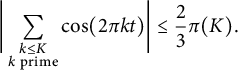
$\cos (2\pi k t) \leq 1/\sqrt {2}$
 for all primes
$3 \leq k \leq \pi K /(8 \sqrt {10})$
for all primes
$3 \leq k \leq \pi K /(8 \sqrt {10})$
 . Combining all the ranges, we conclude that there exists a constant
$C_1>0$
. Combining all the ranges, we conclude that there exists a constant
$C_1>0$
 such that for
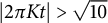
$\lvert 2 \pi K t \rvert> \sqrt {10}$
such that for
$\lvert 2 \pi K t \rvert> \sqrt {10}$
 ,
,

which completes the proof.
Our next lemma shows that if we twist the sums in Lemma 6.2 by quadratic characters, their sizes are typically small. For
$ t \in [-\tfrac {1}{2},\tfrac {1}{2}] $
 , define
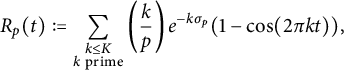
where
$\sigma _p$
 is given by (6.1).
Lemma 6.3 Let
$\eta>2,A>0$
 , and
$B>0$
, and
$B>0$
 be arbitrary constants. Suppose
$X>0$
be arbitrary constants. Suppose
$X>0$
 is sufficiently large in terms of
$\eta ,A$
is sufficiently large in terms of
$\eta ,A$
 , and B, and set
$K=(\log X)^A$
, and B, and set
$K=(\log X)^A$
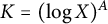 . Let
$t \in [-\tfrac {1}{2},\tfrac {1}{2}]$
. Let
$t \in [-\tfrac {1}{2},\tfrac {1}{2}]$
 such that
$\lvert 2 \pi Kt \rvert> \sqrt {10}$
such that
$\lvert 2 \pi Kt \rvert> \sqrt {10}$
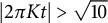 . For each prime
$p \in (X, 2X]$
. For each prime
$p \in (X, 2X]$
 , let
$R_p(t)$
, let
$R_p(t)$
 be as defined in (6.10). Then outside an exceptional set of primes
$\mathcal {E}\subseteq (X, 2X]$
be as defined in (6.10). Then outside an exceptional set of primes
$\mathcal {E}\subseteq (X, 2X]$
 , which depends at most on
$ X, \eta , A, B $
, which depends at most on
$ X, \eta , A, B $
 , and
$ t $
, and
$ t $
 , and satisfies the bound

we have
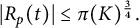
$\lvert R_p(t)\rvert \leq \pi (K)^{\frac {3}{4}}.$
Proof Our approach is to study the high moments of
$R_p(t)$
 , more precisely, the following sum:
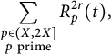
where
$r \in \mathbb {N}$
 is fixed. Expanding the
$2r$
is fixed. Expanding the
$2r$
 -th exponent and using Taylor expansion, we have
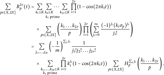
Let
$J_0>0$
 be a large parameter depending only on
$\eta $
be a large parameter depending only on
$\eta $
 and r. We consider the following cases.
Case 1:
$0 \leq \sum _{i}j_i = J \leq J_0$
 . Note that
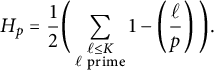
Therefore, the contribution from this case to (6.11) equals
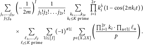
When the product
$\prod _{i=1}^{2r} k_i \cdot \prod _{u\in \mathcal {U}} \ell _u$
 is not a perfect square, by Lemma 4.1, for any
$B_0>0$
is not a perfect square, by Lemma 4.1, for any
$B_0>0$
 ,
,

Choosing
$B_0$
 large depending at most on
$\eta ,A$
large depending at most on
$\eta ,A$
 , and r, the contribution here is
$\ll _{\eta ,A,r} X (\log X)^{-1}$
, and r, the contribution here is
$\ll _{\eta ,A,r} X (\log X)^{-1}$
 .
.
Now suppose
$\prod _{i=1}^{2r} k_i \cdot \prod _{u\in \mathcal {U}} \ell _u$
 is a perfect square. This forces
$\#\mathcal {U}$
is a perfect square. This forces
$\#\mathcal {U}$
 to be even. Then (6.12) equals
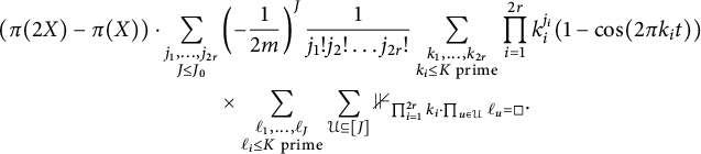
The count of cases where the product is a perfect square is
$\ll _{\eta ,A,r} \pi (K)^{r+\#\mathcal {U}/2}$
 following the proof of Lemma 4.2. When
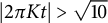
$\lvert 2 \pi Kt \rvert> \sqrt {10}$
following the proof of Lemma 4.2. When
$\lvert 2 \pi Kt \rvert> \sqrt {10}$
 , using the trivial bound
$1-\cos (2\pi k_i t) \leq 1$
, using the trivial bound
$1-\cos (2\pi k_i t) \leq 1$
 and
$\eta>2$
and
$\eta>2$
 , (6.14) is

Case 2:
$\sum _{i}j_i = J> J_0$
 . Since
$H_p \leq \pi (K)$
. Since
$H_p \leq \pi (K)$
 , the contribution from these cases to (6.11) is

by allowing
$J_0 \geq r \cdot (\eta -2)^{-1}$
 .
.
We combine both cases and the bounds (6.15)–(6.16). Choosing
$J_0=\lceil r \cdot (\eta -2)^{-1} \rceil $
 , we obtain

For
$t \in [-\tfrac {1}{2},\tfrac {1}{2}]$
 with
$\lvert 2 \pi K t \rvert> \sqrt {10}$
with
$\lvert 2 \pi K t \rvert> \sqrt {10}$
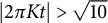 , define

By (6.17), we have

Choosing r sufficiently large in terms of A and B, we see that
$\#\mathcal {E}(t) \ll _{\eta ,A,B} X(\log X)^{-B}$
 .
.
Remark 6.1. In (6.18), it is sufficient to choose any exponent exceeding
$ \frac {1}{2} $
 .
.
The exceptional set derived from Lemma 6.3 depends on the continuous variable
$ t $
 . We now discretize this dependence by showing that small deviations in
$ t $
. We now discretize this dependence by showing that small deviations in
$ t $
 have minimal impact on
$ R_p(t) $
have minimal impact on
$ R_p(t) $
 .
.
Lemma 6.4 Let the notations be as in Lemma 6.3. Then outside an exceptional set of primes
$\mathcal {E} \subseteq (X, 2X]$
 , which depends at most on
$ X, \eta , A$
, which depends at most on
$ X, \eta , A$
 , and
$ B $
, and
$ B $
 , and satisfies the bound

we have the uniform bounds
$H_p \geq \frac {\pi (K)}{3}$
 and
and

Proof As in the proof of Lemma 6.1, we restrict ourselves to primes from the set
$(X,2X] \setminus \mathcal {F}$
 , where
$\mathcal {F}$
, where
$\mathcal {F}$
 is as in (6.2). This ensures the uniform bound
$H_p \geq \frac {\pi (K)}{3}$
is as in (6.2). This ensures the uniform bound
$H_p \geq \frac {\pi (K)}{3}$
 . By the mean value theorem, if
$t_1,t_2 \in [-\tfrac {1}{2}, \tfrac {1}{2}]$
. By the mean value theorem, if
$t_1,t_2 \in [-\tfrac {1}{2}, \tfrac {1}{2}]$
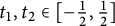 with
$\lvert t_1 -t_2 \rvert \leq T^{-1}$
with
$\lvert t_1 -t_2 \rvert \leq T^{-1}$
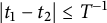 for some
$T>0$
for some
$T>0$
 , then
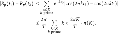
We choose
$T= \lceil K^2\rceil $
 and divide the interval
$(\frac {\sqrt {10}}{2 \pi K}, \frac {1}{2}]$
and divide the interval
$(\frac {\sqrt {10}}{2 \pi K}, \frac {1}{2}]$
 into sub-intervals
$I_1,I_2, \dots $
into sub-intervals
$I_1,I_2, \dots $
 of length
$T^{-1}$
of length
$T^{-1}$
 . Note that there are at most T such sub-intervals. For each sub-interval
$I_j$
. Note that there are at most T such sub-intervals. For each sub-interval
$I_j$
 , define

Consider a prime
$p \in \mathcal {E}_j$
 . Let
$t_1 \in I_j$
. Let
$t_1 \in I_j$
 such that
$\lvert R_p(t_1)\rvert> 2 \cdot \pi (K)^{\frac {3}{4}}$
such that
$\lvert R_p(t_1)\rvert> 2 \cdot \pi (K)^{\frac {3}{4}}$
 . Then by (6.19) and the triangle inequality, for any
$t_2 \in I_j$
. Then by (6.19) and the triangle inequality, for any
$t_2 \in I_j$
 , we have

It follows that
$p \in \mathcal {E}(t_2)$
 , where
$\mathcal {E}(t_2)$
, where
$\mathcal {E}(t_2)$
 is given by (6.18). Therefore, we have
$\# \mathcal {E}_j \subseteq \mathcal {E}(t_2)$
is given by (6.18). Therefore, we have
$\# \mathcal {E}_j \subseteq \mathcal {E}(t_2)$
 and by Lemma 6.3, we obtain the bound
$\# \mathcal {E}_j \ll _{\eta ,A,B_0} X (\log X)^{-B_0}$
and by Lemma 6.3, we obtain the bound
$\# \mathcal {E}_j \ll _{\eta ,A,B_0} X (\log X)^{-B_0}$
 for any
$B_0>0$
for any
$B_0>0$
 . Taking the union over all j’s, we deduce that

by choosing
$B_0$
 sufficiently large depending on
$\eta ,A$
sufficiently large depending on
$\eta ,A$
 , and B. A similar argument gives rise to analogous exceptional sets for the interval
$[-\frac {1}{2},-\frac {\sqrt {10}}{2 \pi K})$
, and B. A similar argument gives rise to analogous exceptional sets for the interval
$[-\frac {1}{2},-\frac {\sqrt {10}}{2 \pi K})$
 . Letting
$\mathcal {E}$
. Letting
$\mathcal {E}$
 be the union of these exceptional sets
$\mathcal {E}_j$
be the union of these exceptional sets
$\mathcal {E}_j$
 ’s along with
$\mathcal {F}$
’s along with
$\mathcal {F}$
 , we arrive at the desired conclusion.
Combining Lemmas 6.1, 6.2, and 6.4, we arrive at the following corollary which establishes an upper bound for
$\log f_p(\tau )$
 for almost all primes, when
$ \tfrac {\pi }{4} < \lvert \operatorname {Arg}(\tau ) \rvert \leq \tfrac {\pi }{2} $
for almost all primes, when
$ \tfrac {\pi }{4} < \lvert \operatorname {Arg}(\tau ) \rvert \leq \tfrac {\pi }{2} $
 .
.
Corollary 6.5 Let the notations be as in Lemma 6.1. There exists a constant
$C_2>0$
 such that outside an exceptional set of primes
$\mathcal {E} \subseteq (X, 2X]$
such that outside an exceptional set of primes
$\mathcal {E} \subseteq (X, 2X]$
 , which depends at most on
$ X, \eta ,A$
, which depends at most on
$ X, \eta ,A$
 , and
$B $
, and
$B $
 , and satisfies

we have the uniform bounds
$H_p \geq \frac {\pi (K)}{3}$
 and
and

Proof Let
$\mathcal {E}$
 be the exceptional set provided by Lemma 6.4. Since
$\mathcal {F} \subseteq \mathcal {E}$
be the exceptional set provided by Lemma 6.4. Since
$\mathcal {F} \subseteq \mathcal {E}$
 where
$\mathcal {F}$
where
$\mathcal {F}$
 is as in (6.2), we obtain the uniform bound
$H_p \geq \frac {\pi (K)}{3}$
is as in (6.2), we obtain the uniform bound
$H_p \geq \frac {\pi (K)}{3}$
 for all
$p \in (X,2X]\setminus \mathcal {E}$
for all
$p \in (X,2X]\setminus \mathcal {E}$
 . Furthermore, by Lemma 6.1, for all
$p \in (X,2X]\setminus \mathcal {E}$
. Furthermore, by Lemma 6.1, for all
$p \in (X,2X]\setminus \mathcal {E}$
 , we have

for some constant
$C_0>0$
 . To handle the remaining range, note that by (6.3),

where
$R_p(t)$
 is given by (6.10). By Lemmas 6.2 and 6.4, for all
$p \in (X,2X]\setminus \mathcal {E}$
is given by (6.10). By Lemmas 6.2 and 6.4, for all
$p \in (X,2X]\setminus \mathcal {E}$
 , the right-hand side of (6.20) is
$\leq -\frac {C_1}{2} \pi (K)$
, the right-hand side of (6.20) is
$\leq -\frac {C_1}{2} \pi (K)$
 , where
$ C_1> 0 $
, where
$ C_1> 0 $
 is the constant from Lemma 6.2. Hence, we deduce that

Combining the two ranges and choosing
$C_2 = \min \{ C_0,C_1/2 \}$
 , we arrive at the desired result.
7 Proofs of Theorems 1.1 and 1.2
7.1 Proof of Theorem 1.1
To establish Theorem 1.1, our starting point is the relation (2.2):

We will use the saddle point method to estimate the integral. For each prime
$p \in (X, 2X]$
 , our choice of
$\sigma $
, our choice of
$\sigma $
 , as discussed in Section 6, is
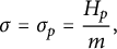
where
$H_p$
 is given by (5.1). In what follows, we will only work with primes outside the exceptional set
$\mathcal {E}$
is given by (5.1). In what follows, we will only work with primes outside the exceptional set
$\mathcal {E}$
 provided by Corollary 6.5. This ensures that
$H_p \geq \frac {\pi (K)}{3}$
provided by Corollary 6.5. This ensures that
$H_p \geq \frac {\pi (K)}{3}$
 . Let
$\eta>3$
. Let
$\eta>3$
 and
and
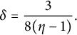
We break
$\mathcal {P}_{\mathbb {H}_p}(m)$
 by
by

where


Analysis for I. Let
$\tau = \sigma _p+2\pi i t$
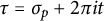 . In our range of integration,
$0 \leq \lvert \operatorname {Arg}(\tau ) \rvert \leq \tfrac {\pi }{4}$
. In our range of integration,
$0 \leq \lvert \operatorname {Arg}(\tau ) \rvert \leq \tfrac {\pi }{4}$
 . We choose
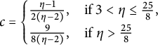
in Lemma 5.1. Then for all
$p \in (X, 2X]\setminus \mathcal {E}$
 , we have

uniformly for
$\lvert t \rvert \leq \sigma _p^{1+\delta }$
 . Furthermore, we have the Taylor series expansion

Substituting (7.1), (7.6), and (7.7) in (7.4), we have
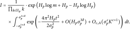
After a change of variables
$t=\kappa u$
 with
$\kappa = \sigma _p/(2\pi \sqrt {H_p})$
with
$\kappa = \sigma _p/(2\pi \sqrt {H_p})$
 , we see that

We substitute this in (7.8) and apply Stirling’s formula. Putting together the values of
$\delta $
 , c, and
$\kappa $
, c, and
$\kappa $
 , we have for any
$\varepsilon>0$
, we have for any
$\varepsilon>0$
 ,
,

Analysis for E. Regarding the term E, we consider the following two cases.
Case 1:
$ \lvert \operatorname {Arg}(\tau ) \rvert \leq \frac {\pi }{4}$
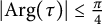 . Again, let
$\tau = \sigma _p+2\pi i t$
. Again, let
$\tau = \sigma _p+2\pi i t$
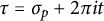 . We will apply Lemma 5.1 here. If
$\sigma _p^{1+\delta }<|t|<\frac {\sigma _p}{10}$
. We will apply Lemma 5.1 here. If
$\sigma _p^{1+\delta }<|t|<\frac {\sigma _p}{10}$
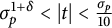 , then using the expansion
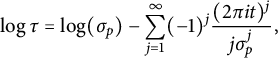
we obtain

for some constant
$c_1>0$
 . On the other hand, if
$\frac {\sigma _p}{10}\leq |t| \leq \frac {\sigma _p}{2\pi }$
. On the other hand, if
$\frac {\sigma _p}{10}\leq |t| \leq \frac {\sigma _p}{2\pi }$
 , then we have
$(1+c_2)\sigma _p \leq \lvert \tau \rvert $
, then we have
$(1+c_2)\sigma _p \leq \lvert \tau \rvert $
 for some constant
$c_2>0$
for some constant
$c_2>0$
 . This implies that

for some constant
$c_3>0$
 . Overall, by Lemma 5.1, in this case, for all
$p \in (X, 2X]\setminus \mathcal {E}$
. Overall, by Lemma 5.1, in this case, for all
$p \in (X, 2X]\setminus \mathcal {E}$
 ,
,

for some constant
$c_4>0$
 . Substituting the value of
$\delta $
. Substituting the value of
$\delta $
 from (7.2), we can conclude that

Case 2:
$ \frac {\pi }{4} \leq \lvert \operatorname {Arg}(\tau ) \rvert \leq \frac {\pi }{2}$
 . Here, we have
$\frac {\sigma _p}{2\pi } <|t|\leq \frac {1}{2}$
. Here, we have
$\frac {\sigma _p}{2\pi } <|t|\leq \frac {1}{2}$
 and we will use Corollary 6.5. We write
$\tau = \sigma _p+2\pi i t$
and we will use Corollary 6.5. We write
$\tau = \sigma _p+2\pi i t$
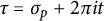 . By Corollary 6.5, for all
$p \in (X, 2X]\setminus \mathcal {E}$
. By Corollary 6.5, for all
$p \in (X, 2X]\setminus \mathcal {E}$
 ,
,

for some constant
$C_2>0$
 .
.
Substituting the bounds (7.11) and (7.12) in (7.5) and integrating, we see that the error term E can be absorbed into the error term arising from I. It follows that

This completes the proof of Theorem 1.1.
7.2 Proof of Theorem 1.2
By Theorem 1.1, for j sufficiently large depending on
$\eta $
 and A, we have

for all primes
$p \in (X_j,2X_j]$
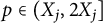 outside an exceptional set
$\mathcal {E}_j \subseteq (X_j,2X_j]$
outside an exceptional set
$\mathcal {E}_j \subseteq (X_j,2X_j]$
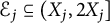 satisfying

say. Taking logarithms on both sides of (7.13), we see that for all primes
$p \in (X_j,2X_j] \setminus \mathcal {E}_j$
 ,
,
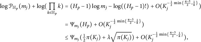
if
$H_p \leq \tfrac {1}{2}\pi (K_j) +\lambda \sqrt {\pi (K_j)}$
 . The last inequality holds since
$\Psi _{m_j}(t)$
. The last inequality holds since
$\Psi _{m_j}(t)$
 is increasing in t. Letting
$j \to \infty $
is increasing in t. Letting
$j \to \infty $
 , we see that the set of primes
$p \in (X_j,2X_j] \setminus \mathcal {E}_j$
, we see that the set of primes
$p \in (X_j,2X_j] \setminus \mathcal {E}_j$
 for which (7.15) holds is the same as the set

Now, using Lemma 4.3 and (7.14), we arrive at the desired conclusion.
Remark 7.1. The restriction
$ \eta> 3 $
 arises from the requirement that
$ c \in (0,1) $
arises from the requirement that
$ c \in (0,1) $
 in Lemma 5.1. While the analysis in Section 6 remains valid for
$ \eta> 2 $
in Lemma 5.1. While the analysis in Section 6 remains valid for
$ \eta> 2 $
 , reducing the threshold for
$\eta $
, reducing the threshold for
$\eta $
 would necessitate taking
$ c> 1 $
would necessitate taking
$ c> 1 $
 . This, in turn, would require shifting the contour of integration further to the left in the proof of Lemma 5.1, thereby enclosing additional poles of the integrand at
$ s = -1, -2n $
. This, in turn, would require shifting the contour of integration further to the left in the proof of Lemma 5.1, thereby enclosing additional poles of the integrand at
$ s = -1, -2n $
 for
$ n \in \mathbb {N} $
for
$ n \in \mathbb {N} $
 . Understanding the contributions from these new residues calls for a detailed investigation into the statistical behavior of the function
$ \mathcal {D}_p(s) $
. Understanding the contributions from these new residues calls for a detailed investigation into the statistical behavior of the function
$ \mathcal {D}_p(s) $
 for such values of s, in particular, sums of the form
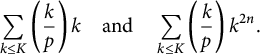
Analyzing such expressions may possibly lead to an improvement in the admissible range of
$ \eta $
 , and consequently reveal secondary lower-order terms in the distribution of the partition function
$ \mathcal {P}_{\mathbb {H}_p}(m) $
, and consequently reveal secondary lower-order terms in the distribution of the partition function
$ \mathcal {P}_{\mathbb {H}_p}(m) $
 . This would be along the lines of Szekeres’ work [Reference Szekeres38, Reference Szekeres39] on unrestricted partitions in the sense that each part is allowed to take any value up to
$ K $
. This would be along the lines of Szekeres’ work [Reference Szekeres38, Reference Szekeres39] on unrestricted partitions in the sense that each part is allowed to take any value up to
$ K $
 without any additional arithmetic constraints.
8 The character twist aspect: Proofs of Theorems 1.3 and 1.4
Let the notations be as in Section 1. Given an odd prime q, for each prime
$p \in (X, 2X]$
 , recall that

We also defined

Let
$\tau = \sigma + 2 \pi i t$
 , where
$\sigma , t \in \mathbb {R}$
, where
$\sigma , t \in \mathbb {R}$
 with
$\sigma> 0$
with
$\sigma> 0$
 . The generating function we consider here is

where
$w = e^{-\tau }$
 . We present the following results, which are analogous to those corresponding to Theorems 1.1 and 1.2. Since the proofs are similar, we focus only on highlighting some necessary differences for the benefit of the reader. The character sums to study here are
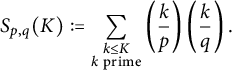
Lemma 8.1 Let
$ A> 0 $
 be an arbitrary constant and q be a fixed odd prime. Suppose
$ X> 0 $
be an arbitrary constant and q be a fixed odd prime. Suppose
$ X> 0 $
 is sufficiently large in terms of A and q, and set
$K=(\log X)^A$
is sufficiently large in terms of A and q, and set
$K=(\log X)^A$
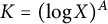 . For each prime
$ p \in (X, 2X] $
. For each prime
$ p \in (X, 2X] $
 , let
$ S_{p,q}(K) $
, let
$ S_{p,q}(K) $
 be defined by (8.4). Fix
$ r \in \mathbb {N} $
be defined by (8.4). Fix
$ r \in \mathbb {N} $
 . Then, for any
$ B> 0 $
. Then, for any
$ B> 0 $
 , we have
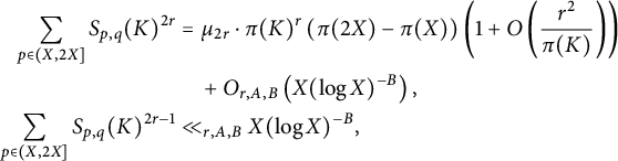
where
$ \mu _{2r} = (2r-1) \dots 3 \cdot 1 $
 is the
$ 2r $
is the
$ 2r $
 -th moment of a standard Gaussian. Moreover, for any
$\lambda \in \mathbb {R}$
-th moment of a standard Gaussian. Moreover, for any
$\lambda \in \mathbb {R}$
 ,
,

For the main term in Theorem 1.3, we need the following lemma.
Lemma 8.2 Let
$c\in (0,1)$
 and
$A>0$
and
$A>0$
 be arbitrary constants. Let q be a fixed odd prime. Let
$\tau = \sigma + 2\pi i t$
be arbitrary constants. Let q be a fixed odd prime. Let
$\tau = \sigma + 2\pi i t$
 , where
$\left | \operatorname {Arg}(\tau ) \right | \leq \frac {\pi }{4}$
, where
$\left | \operatorname {Arg}(\tau ) \right | \leq \frac {\pi }{4}$
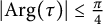 and
$\sigma , t \in \mathbb {R}$
and
$\sigma , t \in \mathbb {R}$
 satisfy
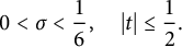
Suppose
$X>0$
 is sufficiently large in terms of
$c,A$
is sufficiently large in terms of
$c,A$
 , and q, and set
$K=(\log X)^A$
, and q, and set
$K=(\log X)^A$
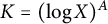 . For each prime
$p \in (X, 2X]$
. For each prime
$p \in (X, 2X]$
 , let
$f_{p,q}(\tau )$
, let
$f_{p,q}(\tau )$
 be defined by (8.3). Then uniformly for
$\lvert t \rvert \leq \frac {1}{2} $
be defined by (8.3). Then uniformly for
$\lvert t \rvert \leq \frac {1}{2} $
 ,
,

Proof The proof follows the arguments in Lemma 5.1.
We now proceed toward bounding the error terms. For each prime
$ p \in (X, 2X] $
 , we define
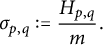
Lemma 8.3 Let
$\eta>2,A>0$
 , and
$B>0$
, and
$B>0$
 be arbitrary constants. Let q be a fixed odd prime. Suppose
$X>0$
be arbitrary constants. Let q be a fixed odd prime. Suppose
$X>0$
 is sufficiently large in terms of
$\eta ,A,B$
is sufficiently large in terms of
$\eta ,A,B$
 , and q, and set
$K=(\log X)^A$
, and q, and set
$K=(\log X)^A$
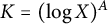 . For each prime
$p \in (X, 2X]$
. For each prime
$p \in (X, 2X]$
 , let
$f_{p,q}(\tau )$
, let
$f_{p,q}(\tau )$
 be defined by (8.3) and
$\sigma _{p,q}$
be defined by (8.3) and
$\sigma _{p,q}$
 be as in (8.6). There exists a constant
$C_2>0$
be as in (8.6). There exists a constant
$C_2>0$
 such that outside an exceptional set of primes
$\mathcal {E} \subseteq (X, 2X]$
such that outside an exceptional set of primes
$\mathcal {E} \subseteq (X, 2X]$
 , which depends at most on
$ X, \eta ,A,B$
, which depends at most on
$ X, \eta ,A,B$
 , and
$q $
, and
$q $
 , and satisfies

we have the uniform bounds
$H_{p,q} \geq \frac {\pi (K)}{3}$
 and
and

Proof The range
$\frac {\sigma _{p,q}}{2\pi }< \lvert t \rvert \leq \frac {\sqrt {10}}{2 \pi K}$
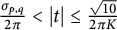 can be handled precisely following the arguments of Lemma 6.1. In particular, there exists a constant
$C_0>0$
can be handled precisely following the arguments of Lemma 6.1. In particular, there exists a constant
$C_0>0$
 such that outside an exceptional set of primes
$\mathcal {F} \subseteq (X, 2X]$
such that outside an exceptional set of primes
$\mathcal {F} \subseteq (X, 2X]$
 given by

which depends at most on
$ X, \eta ,A$
 , and
$q $
, and
$q $
 , and satisfies

we have the uniform bounds
$H_{p,q} \geq \frac {\pi (K)}{3}$
 and
and

We now present an alternative approach toward handling the remaining range
$ \frac {\sqrt {10}}{2 \pi K} < \lvert t \rvert \leq \frac {1}{2} $
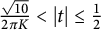 . Instead of estimating high moments and applying the discretization method as in Section 6, we use the Erdős–Turán inequality [Reference Montgomery33, Chapter 1, Corollary 1.1]. Throughout the remainder of the proof, we restrict ourselves to working with primes from the set
$(X,2X]\setminus \mathcal {F}$
. Instead of estimating high moments and applying the discretization method as in Section 6, we use the Erdős–Turán inequality [Reference Montgomery33, Chapter 1, Corollary 1.1]. Throughout the remainder of the proof, we restrict ourselves to working with primes from the set
$(X,2X]\setminus \mathcal {F}$
 . Let
$\varepsilon _0>0$
. Let
$\varepsilon _0>0$
 be an arbitrarily small absolute constant. For t satisfying
$ \frac {\sqrt {10}}{2 \pi K} < \lvert t \rvert \leq \frac {1}{2} $
be an arbitrarily small absolute constant. For t satisfying
$ \frac {\sqrt {10}}{2 \pi K} < \lvert t \rvert \leq \frac {1}{2} $
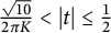 , let
, let

If
$H_{p,q}(t) < \tfrac {\pi (K)}{4}$
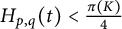 for all t in our range and all
$p \in (X,2X]\setminus \mathcal {F}$
for all t in our range and all
$p \in (X,2X]\setminus \mathcal {F}$
 , then we have

for some constant
$C_1>0$
 depending only on
$\varepsilon _0$
depending only on
$\varepsilon _0$
 . This implies (8.7). So we may assume that for some t in our range and for some prime
$p \in (X,2X]\setminus \mathcal {F}$
. This implies (8.7). So we may assume that for some t in our range and for some prime
$p \in (X,2X]\setminus \mathcal {F}$
 ,
$H_{p,q}(t) \geq \tfrac {\pi (K)}{4}$
,
$H_{p,q}(t) \geq \tfrac {\pi (K)}{4}$
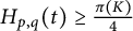 . We now proceed along the following steps to arrive at a contradiction to this assumption. The key argument is that
$\pi (K)/4$
. We now proceed along the following steps to arrive at a contradiction to this assumption. The key argument is that
$\pi (K)/4$
 many primes cannot have
$\cos (2\pi kt)$
many primes cannot have
$\cos (2\pi kt)$
 so close to
$1$
so close to
$1$
 .
.
Step 1: Consider the sequence
$ \{ k t \bmod 1 \}$
 , as k varies over the primes up to K. Denote by
$\mathscr {D}$
, as k varies over the primes up to K. Denote by
$\mathscr {D}$
 , the discrepancy of this sequence, which is defined by

We choose
$\alpha _1=-(2 \pi )^{-1}\cos ^{-1}(1-\varepsilon _0)$
 and
$\alpha _2 =(2 \pi )^{-1}\cos ^{-1}(1-\varepsilon _0)$
and
$\alpha _2 =(2 \pi )^{-1}\cos ^{-1}(1-\varepsilon _0)$
 . It follows that

by choosing
$\varepsilon _0$
 small enough. On the other hand, by the Erdős–Turán inequality, for any
$H \in \mathbb {N}$
small enough. On the other hand, by the Erdős–Turán inequality, for any
$H \in \mathbb {N}$
 ,
,
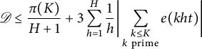
for each
$1 \leq h \leq H$
 , there exists a reduced fraction
$u_h/v_h$
, there exists a reduced fraction
$u_h/v_h$
 with
$0 \leq u_h < v_h$
with
$0 \leq u_h < v_h$
 and
$1 \leq v_h \leq K_1$
and
$1 \leq v_h \leq K_1$
 such that
$\lvert \{ht\} -u_h/v_h\rvert \leq 1/(v_hK_1) \leq 1/v_h^2$
such that
$\lvert \{ht\} -u_h/v_h\rvert \leq 1/(v_hK_1) \leq 1/v_h^2$
 . If
$v_h \geq (\log K)^{10}$
. If
$v_h \geq (\log K)^{10}$
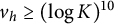 for some h, then by (6.9) and partial summation, we find that
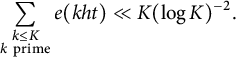
On the other hand, if
$300 < v_h \leq (\log K)^{10}$
 for some h, then writing
$\{ht\}=u_h/v_h+\beta _h$
for some h, then writing
$\{ht\}=u_h/v_h+\beta _h$
 , we have

for any
$B>0$
 , where
$T(\beta _h) = \sum _{k \leq K} e(k \beta _h)$
, where
$T(\beta _h) = \sum _{k \leq K} e(k \beta _h)$
 . Trivially bounding
$T(\beta _h)$
. Trivially bounding
$T(\beta _h)$
 and using partial summation,
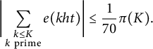
Finally, if
$1 \leq v_h \leq 300$
 but
$36/K \leq \lvert \beta _h \rvert \leq 1/(v_h K_1) $
but
$36/K \leq \lvert \beta _h \rvert \leq 1/(v_h K_1) $
 , then similar to the proof of Lemma 6.2, instead of trivially bounding
$T(\beta _h)$
, then similar to the proof of Lemma 6.2, instead of trivially bounding
$T(\beta _h)$
 , we use the sharper bound
$\lvert T(\beta _h) \rvert \leq \lvert \sin (\pi \beta _h) \rvert ^{-1}$
, we use the sharper bound
$\lvert T(\beta _h) \rvert \leq \lvert \sin (\pi \beta _h) \rvert ^{-1}$
 to obtain
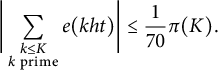
In conclusion, if t is such that for all
$1 \leq h \leq H$
 ,
$v_h>300$
,
$v_h>300$
 , or
$36/K \leq \lvert \beta _h \rvert \leq 1/(v_h K_1)$
, or
$36/K \leq \lvert \beta _h \rvert \leq 1/(v_h K_1)$
 , then substituting the bounds (8.12)–(8.14) in (8.11), and evaluating the harmonic sum, we see that
$\mathscr {D} < \frac {\pi (K)}{5}$
, then substituting the bounds (8.12)–(8.14) in (8.11), and evaluating the harmonic sum, we see that
$\mathscr {D} < \frac {\pi (K)}{5}$
 , which contradicts (8.10), and thereby, contradicts the assumption that
$H_{p,q}(t) \geq \tfrac {\pi (K)}{4}$
, which contradicts (8.10), and thereby, contradicts the assumption that
$H_{p,q}(t) \geq \tfrac {\pi (K)}{4}$
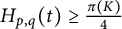 .
.
Step 2: Following Step 1, we may now assume that for some
$1 \leq h \leq H$
 , we have
$1 \leq v_h \leq 300$
, we have
$1 \leq v_h \leq 300$
 and
$\lvert \beta _h \rvert \leq 36/K$
and
$\lvert \beta _h \rvert \leq 36/K$
 . Note that
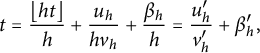
where
$\beta _h^{\prime } = \beta _h/h$
 and
$(u_h^{\prime }, v_h^{\prime })=1$
and
$(u_h^{\prime }, v_h^{\prime })=1$
 . For
$1 \leq b \leq v_h^{\prime }$
. For
$1 \leq b \leq v_h^{\prime }$
 with
$(b,v_h^{\prime })=1$
with
$(b,v_h^{\prime })=1$
 , consider the set
$\{ k \in \mathbb {H}_{p,q}(t) : k \equiv b \bmod v_h^{\prime }\}.$
, consider the set
$\{ k \in \mathbb {H}_{p,q}(t) : k \equiv b \bmod v_h^{\prime }\}.$
 Then our assumption
$H_{p,q}(t) \geq \tfrac {\pi (K)}{4}$
Then our assumption
$H_{p,q}(t) \geq \tfrac {\pi (K)}{4}$
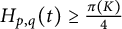 implies that there exists some b for which

We will contradict (8.16). To see this, let
$k \in \mathbb {H}_{p,q}(t)$
 with
$k \equiv b \bmod v_h^{\prime }$
with
$k \equiv b \bmod v_h^{\prime }$
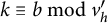 . Using (8.15), we have

Writing
$n_{k,h}$
 to be the closest integer to
$bu_h^{\prime }/v_h^{\prime }+k \beta _h^{\prime }$
to be the closest integer to
$bu_h^{\prime }/v_h^{\prime }+k \beta _h^{\prime }$
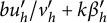 , it follows that

for some constant
$c_0>0$
 . Hence, we deduce that

To conclude the argument, first consider the range
$1/(3Kv_h^{\prime }) \leq \lvert \beta _h^{\prime } \rvert \leq 36/(Kh)$
 . By (8.18) and the Siegel–Walfisz theorem, we have

By choosing
$\varepsilon _0$
 sufficiently small, this contradicts (8.16). On the other hand, if
$\lvert \beta _h^{\prime } \rvert <1/(3Kv_h^{\prime })$
sufficiently small, this contradicts (8.16). On the other hand, if
$\lvert \beta _h^{\prime } \rvert <1/(3Kv_h^{\prime })$
 , then choosing
$\varepsilon _0$
, then choosing
$\varepsilon _0$
 small enough such that
$\varepsilon _0 < 10 \cdot 5700^{-2} \leq 10 v_h^{\prime -2}$
small enough such that
$\varepsilon _0 < 10 \cdot 5700^{-2} \leq 10 v_h^{\prime -2}$
 , we see that no k satisfies (8.17), and we again arrive at a contradiction.
We combine Steps 1 and 2 to conclude that (8.9) holds for all t in our range and all
$p \in (X,2X]\setminus \mathcal {F}$
 . From here on, we can follow the argument in Corollary 6.5 to arrive at our desired conclusion.
The proof of Theorem 1.3 now follows from the same reasoning as in Theorem 1.1, incorporating Lemmas 8.2 and 8.3. The proof of Theorem 1.4 then proceeds analogously to that of Theorem 1.2, relying in particular on Lemma 8.1.
9 The arithmetic progression aspect: Proof of Theorem 1.5
Let the notations be as in Section 1. Fix a prime D and let
$b \in (\mathbb {Z}/D\mathbb {Z})^{\times }$
 . For each prime
$p \in (X, 2X]$
. For each prime
$p \in (X, 2X]$
 , recall that

We also defined

Let
$\tau = \sigma + 2 \pi i t$
 , where
$\sigma , t \in \mathbb {R}$
, where
$\sigma , t \in \mathbb {R}$
 with
$\sigma> 0$
with
$\sigma> 0$
 . The generating function we consider here is

where
$w = e^{-\tau }$
 . We present the following results, which are analogous to those corresponding to Theorem 1.1. The main difference in the arithmetic progression case lies in performing a more careful analysis of the error terms. The main terms corresponding to Theorem 1.5 are obtained in the same fashion as in Lemma 5.1.
Lemma 9.1 Let
$c\in (0,1)$
 and
$A>0$
and
$A>0$
 be arbitrary constants. Let D be a fixed prime and
$b \in (\mathbb {Z}/D\mathbb {Z})^{\times }$
be arbitrary constants. Let D be a fixed prime and
$b \in (\mathbb {Z}/D\mathbb {Z})^{\times }$
 . Let
$\tau = \sigma + 2\pi i t$
. Let
$\tau = \sigma + 2\pi i t$
 , where
$\left | \operatorname {Arg}(\tau ) \right | \leq \frac {\pi }{4}$
, where
$\left | \operatorname {Arg}(\tau ) \right | \leq \frac {\pi }{4}$
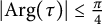 and
$\sigma , t \in \mathbb {R}$
and
$\sigma , t \in \mathbb {R}$
 satisfy
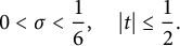
Suppose
$X>0$
 is sufficiently large in terms of
$c,A$
is sufficiently large in terms of
$c,A$
 , and D, and set
$K=(\log X)^A$
, and D, and set
$K=(\log X)^A$
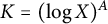 . For each prime
$p \in (X, 2X]$
. For each prime
$p \in (X, 2X]$
 , let
$\widehat {f}_{p}(\tau )$
, let
$\widehat {f}_{p}(\tau )$
 be defined by (9.3). Then uniformly for
$\lvert t \rvert \leq \frac {1}{2} $
be defined by (9.3). Then uniformly for
$\lvert t \rvert \leq \frac {1}{2} $
 ,
,

Proof The proof follows the arguments in Lemma 5.1.
To bound the error terms, for each prime
$ p \in (X, 2X] $
 , we define

Lemma 9.2 Let
$\eta>2,A>0$
 , and
$B>0$
, and
$B>0$
 be arbitrary constants. Let D be a fixed prime and
$b \in (\mathbb {Z}/D\mathbb {Z})^{\times }$
be arbitrary constants. Let D be a fixed prime and
$b \in (\mathbb {Z}/D\mathbb {Z})^{\times }$
 . Suppose
$X>0$
. Suppose
$X>0$
 is sufficiently large in terms of
$\eta ,A,B$
is sufficiently large in terms of
$\eta ,A,B$
 , and D, and set
$K=(\log X)^A$
, and D, and set
$K=(\log X)^A$
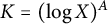 . For each prime
$p \in (X, 2X]$
. For each prime
$p \in (X, 2X]$
 , let
$\widehat {f}_{p}(\tau )$
, let
$\widehat {f}_{p}(\tau )$
 be defined by (9.3) and
$\widehat {\sigma }_p$
be defined by (9.3) and
$\widehat {\sigma }_p$
 be as in (9.5). There exists a constant
$C_0>0$
be as in (9.5). There exists a constant
$C_0>0$
 such that outside an exceptional set of primes
$\mathcal {F} \subseteq (X, 2X]$
such that outside an exceptional set of primes
$\mathcal {F} \subseteq (X, 2X]$
 , which depends at most on
$ X, \eta ,A$
, which depends at most on
$ X, \eta ,A$
 , and
$D $
, and
$D $
 , and satisfies

we have the uniform bounds
$\widehat {H}_{p} \geq \frac {\pi (K;D,b)}{3}$
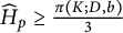 and
and

Proof The proof precisely follows the arguments in Lemma 6.1. The only key difference is, we use the Siegel–Walfisz theorem instead of the prime number theorem.
The analysis for the range
$\frac {\sqrt {10}}{2 \pi K} < \lvert t \rvert \leq \frac {1}{2}$
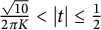 is more subtle. We will require the following variant of Vinogradov’s bound on exponential sums over primes.
Lemma 9.3 Let
$K\geq 1$
 ,
$t \in \mathbb {R}$
,
$t \in \mathbb {R}$
 and consider a reduced fraction
$u/v$
and consider a reduced fraction
$u/v$
 such that
$|t-u/v|\leq \gamma /v^2$
such that
$|t-u/v|\leq \gamma /v^2$
 for some
$\gamma \geq 1$
for some
$\gamma \geq 1$
 . Then

where the implied constant is absolute.
Proof By Dirichlet’s theorem, for any
$t \in \mathbb {R}$
 and for any
$V\geq 1$
and for any
$V\geq 1$
 , there exists a reduced fraction
$u_1/v_1$
, there exists a reduced fraction
$u_1/v_1$
 , where
$1 \leq v_1 \leq V$
, where
$1 \leq v_1 \leq V$
 , and
$(u_1,v_1)=1$
, and
$(u_1,v_1)=1$
 , such that
$\lvert t-u_1/v_1 \rvert \leq 1/(v_1V)\leq 1/v_1^2$
, such that
$\lvert t-u_1/v_1 \rvert \leq 1/(v_1V)\leq 1/v_1^2$
 . Let t be as in the statement of the lemma and
$V=2v$
. Let t be as in the statement of the lemma and
$V=2v$
 . Then
$1\leq v_1\leq 2v$
. Then
$1\leq v_1\leq 2v$
 and
$\lvert t-u_1/v_1 \rvert \leq 1/(2vv_1) \leq 1/v_1^2$
and
$\lvert t-u_1/v_1 \rvert \leq 1/(2vv_1) \leq 1/v_1^2$
 . By (6.9), we have

In the special case, when
$u/v=u_1/v_1$
 , we must have
$u_1=u$
, we must have
$u_1=u$
 and
$v_1=v$
and
$v_1=v$
 . Therefore, (9.7) implies that

Otherwise, assume that
$u/v\neq u_1/v_1$
 . Then we have

This implies that
$1/(2vv_1)\leq \gamma /v^2$
 , which is equivalent to
$v_1^{-\frac {1}{2}} \leq (2\gamma )^{\frac {1}{2}} v^{-\frac {1}{2}}.$
, which is equivalent to
$v_1^{-\frac {1}{2}} \leq (2\gamma )^{\frac {1}{2}} v^{-\frac {1}{2}}.$
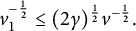 It follows that

Putting together (9.8) and (9.10), we get our desired result.
Lemma 9.4 Let the notations be as in Lemma 9.5. Then there exists a constant
$C_1>0$
 such that the following uniform bound holds:

Proof By partial summation, it suffices to study the sum
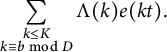
By orthogonality of additive characters, we write

where
$t_{\ell }= t+\ell /D$
 . Let
$K_1 = K(\log K)^{-10}.$
. Let
$K_1 = K(\log K)^{-10}.$
 By Dirichlet’s theorem on Diophantine approximation, there exists a reduced fraction
$u/v$
By Dirichlet’s theorem on Diophantine approximation, there exists a reduced fraction
$u/v$
 with
$1 \leq v \leq K_1$
with
$1 \leq v \leq K_1$
 and
$\lvert t-u/v \rvert \leq 1/(vK_1) \leq 1/v^{2}$
and
$\lvert t-u/v \rvert \leq 1/(vK_1) \leq 1/v^{2}$
 . We write
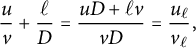
where
$(u_{\ell },v_{\ell })=1$
 . Then
$v_{\ell } \geq v/(v,D)$
. Then
$v_{\ell } \geq v/(v,D)$
 . Furthermore, we have
$\lvert t_{\ell } -u_{\ell }/v_{\ell } \rvert \leq 1/v^2 \leq D^2/v_{\ell }^2$
. Furthermore, we have
$\lvert t_{\ell } -u_{\ell }/v_{\ell } \rvert \leq 1/v^2 \leq D^2/v_{\ell }^2$
 . Therefore, if
$v \geq (\log K)^{10}$
. Therefore, if
$v \geq (\log K)^{10}$
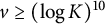 , we apply Lemma 9.3 with
$\gamma = D^2$
, we apply Lemma 9.3 with
$\gamma = D^2$
 to obtain

for all
$0 \leq \ell \leq D-1$
 . Substituting this in (9.12) and using partial summation, we arrive at (9.11). So in what follows, we assume
$1 \leq v < (\log K)^{10}$
. Substituting this in (9.12) and using partial summation, we arrive at (9.11). So in what follows, we assume
$1 \leq v < (\log K)^{10}$
 .
.
Let
$\beta = t-u/v$
 . We write

We detect the exponential phase in (9.14) using the following identity:

where
$\tau (\chi )$
 is the Gauss sum. This yields
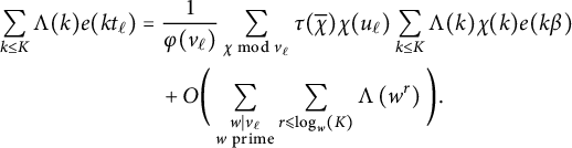
Following [Reference Davenport12, Chapter 26], by partial summation and the Siegel–Walfisz theorem, we see that only the principal character contributes to the main term. In particular, we deduce that for any
$B>0$
 ,
,

where
$T(\beta ) = \sum _{k \leq K} e(k \beta )$
 . Substituting this in (9.12), we arrive at

We now consider the following two cases.
Case 1:
$ (v,D)=1$
 . In this case,
$v_{\ell } = v$
. In this case,
$v_{\ell } = v$
 if
$\ell =0$
if
$\ell =0$
 and
$vD$
and
$vD$
 otherwise. This implies that

Case 2:
$ (v,D)=D$
 . If
$D^2$
. If
$D^2$
 divides v, then
$\mu (v_{\ell })=0$
divides v, then
$\mu (v_{\ell })=0$
 for all
$0 \leq \ell \leq D-1$
for all
$0 \leq \ell \leq D-1$
 , and (9.11) follows trivially. So we may assume that D divides v but
$D^2$
, and (9.11) follows trivially. So we may assume that D divides v but
$D^2$
 doesn’t. In this case,
$v_{\ell } = v/D$
doesn’t. In this case,
$v_{\ell } = v/D$
 if
$\ell \equiv -u \bmod D$
if
$\ell \equiv -u \bmod D$
 and v otherwise. This implies that

We now combine the two cases. If
$v \geq 3$
 in Case 1 or
$v/D \geq 3$
in Case 1 or
$v/D \geq 3$
 in Case 2, then trivially bounding
$T(\beta )$
in Case 2, then trivially bounding
$T(\beta )$
 in (9.15) and using partial summation, we obtain (9.11). Otherwise, if
$\lvert \beta \rvert>\sqrt {10}/(2\pi K)$
in (9.15) and using partial summation, we obtain (9.11). Otherwise, if
$\lvert \beta \rvert>\sqrt {10}/(2\pi K)$
 , we use the more efficient bound
$\lvert T(\beta ) \rvert \leq \pi K/\sqrt {10}.$
, we use the more efficient bound
$\lvert T(\beta ) \rvert \leq \pi K/\sqrt {10}.$
 Finally, we are left with the situation when
$v=1,2$
Finally, we are left with the situation when
$v=1,2$
 in Case 1 or
$v=D,2D$
in Case 1 or
$v=D,2D$
 in Case 2. These can be handled following the arguments in Lemma 6.2.
From here on, we can carry out the method of high moments followed by the discretization argument, as in Section 6. The only differences are notational, and replacing
$\pi (K)$
 by
$\pi (K;D,b)$
by
$\pi (K;D,b)$
 accordingly. We finally arrive at the following corollary, which is an analog of Corollary 6.5.
Corollary 9.5 Let the notations be as in Lemma 9.5. There exists a constant
$C_2>0$
 such that outside an exceptional set of primes
$\mathcal {E}\subseteq (X, 2X]$
such that outside an exceptional set of primes
$\mathcal {E}\subseteq (X, 2X]$
 , which depends at most on
$ X, \eta ,A,B$
, which depends at most on
$ X, \eta ,A,B$
 , and
$D $
, and
$D $
 , and satisfies

we have the uniform bounds
$\widehat {H}_{p} \geq \frac {\pi (K;D,b)}{3}$
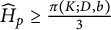 and
and

The proof of Theorem 1.5 now follows from the same reasoning as in Theorem 1.1, incorporating Lemmas 9.1 and 9.5.
10 The Möbius twist aspect: Proof of Theorem 1.6
Let the notations be as in Section 1. For each prime
$p \in (X, 2X]$
 , recall that

We defined

Let
$\tau = \sigma + 2 \pi i t$
 , where
$\sigma , t \in \mathbb {R}$
, where
$\sigma , t \in \mathbb {R}$
 with
$\sigma> 0$
with
$\sigma> 0$
 . The generating function here is

where
$w = e^{-\tau }$
 . The Möbius setting presents two key challenges. First, the distribution of the associated partition function
$ \mathcal {P}_{\mathbb {H}_{p,\mu }}(m) $
. The Möbius setting presents two key challenges. First, the distribution of the associated partition function
$ \mathcal {P}_{\mathbb {H}_{p,\mu }}(m) $
 is not Gaussian, as mentioned in Remark 1.5. Second, to establish Theorem 1.6, we need sharp bounds for exponential sums restricted to square-free integers. We begin by addressing the first point. As in Lemmas 4.2 and 8.1, we shall study sums of the form

Lemma 10.1 Let
$ A> 0 $
 and
$B>0$
and
$B>0$
 be arbitrary constants. Suppose
$ X> 0 $
be arbitrary constants. Suppose
$ X> 0 $
 is sufficiently large in terms of A and B, and set
$K=(\log X)^A$
is sufficiently large in terms of A and B, and set
$K=(\log X)^A$
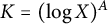 . For each prime
$ p \in (X, 2X] $
. For each prime
$ p \in (X, 2X] $
 , let
$ S_{p,\mu }(K) $
, let
$ S_{p,\mu }(K) $
 be defined by (10.3). Then we have

where
$C_r>0$
 is some absolute constant depending only on r.
Proof We first consider the second moment. Expanding the square and using Lemma 4.1, we have

Observe that when
$k_1,k_2$
 are square-free and their product
$k_1k_2$
are square-free and their product
$k_1k_2$
 is a perfect square, we must have
$k_1=k_2$
is a perfect square, we must have
$k_1=k_2$
 . The desired conclusion follows immediately.
We now focus on the general r-th moment for
$r \geq 3$
 . Here, we will use a result of Harper–Nikeghbali–Radziwiłł [Reference Harper, Nikeghbali and Radziwiłł23] on the moments of a Rademacher random multiplicative function. Expanding the r-th power and using Lemma 4.1, we arrive at
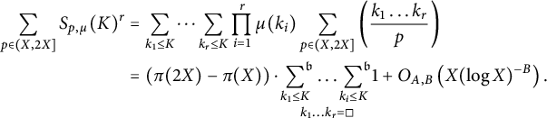
The asymptotics for the sum over
$k_i$
 ’s were established in the proof of [Reference Harper, Nikeghbali and Radziwiłł23, Theorem 1.4]. It is shown that for some constant
$C_r>0$
’s were established in the proof of [Reference Harper, Nikeghbali and Radziwiłł23, Theorem 1.4]. It is shown that for some constant
$C_r>0$
 depending on r, we have

The key thing to observe in Lemma 10.1 is that the moments are not Gaussian. Thus, the analog of Theorem 1.2 fails in this case. The main term for Theorem 1.6 is obtained as in Theorem 1.1.
Lemma 10.2 Let
$c\in (0,1)$
 and
$A>0$
and
$A>0$
 be arbitrary constants. Let
$\tau = \sigma + 2\pi i t$
be arbitrary constants. Let
$\tau = \sigma + 2\pi i t$
 , where
$\left | \operatorname {Arg}(\tau ) \right | \leq \frac {\pi }{4}$
, where
$\left | \operatorname {Arg}(\tau ) \right | \leq \frac {\pi }{4}$
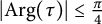 and
$\sigma , t \in \mathbb {R}$
and
$\sigma , t \in \mathbb {R}$
 satisfy
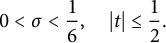
Suppose
$X>0$
 is sufficiently large in terms of c and A, and set
$K=(\log X)^A$
is sufficiently large in terms of c and A, and set
$K=(\log X)^A$
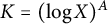 . For each prime
$p \in (X, 2X]$
. For each prime
$p \in (X, 2X]$
 , let
$f_{p,\mu }(\tau )$
, let
$f_{p,\mu }(\tau )$
 be defined by (10.2). Then uniformly for
$\lvert t \rvert \leq \frac {1}{2} $
be defined by (10.2). Then uniformly for
$\lvert t \rvert \leq \frac {1}{2} $
 ,
,

Proof The proof follows the arguments in Lemma 5.1.
To handle the error terms, we require sharp bounds on exponential sums over square-free integers. We first collect the following estimate for counting square-free numbers in arithmetic progressions.
Lemma 10.3 Let
$K \geq 1$
 and
$\varepsilon>0$
and
$\varepsilon>0$
 . Then for
$(b, D)=1$
. Then for
$(b, D)=1$
 , we have

Proof See [Reference Hooley24, Theorem 3].
We now establish bounds for exponential sums over square-free integers. This result sharpens the bound of Schlage–Puchta [Reference Schlage-Puchta37, Theorem 3] in certain ranges of t.
Lemma 10.4 Let
$\theta _1>0$
 and
$\theta _2>0$
and
$\theta _2>0$
 be constants satisfying
$\theta _1+\theta _2<1$
be constants satisfying
$\theta _1+\theta _2<1$
 . Let
$\varepsilon>0$
. Let
$\varepsilon>0$
 and
$K \geq 1$
and
$K \geq 1$
 be sufficiently large in terms of
$\theta _1,\theta _2$
be sufficiently large in terms of
$\theta _1,\theta _2$
 , and
$\varepsilon $
, and
$\varepsilon $
 . Let
$t \in \mathbb {R}$
. Let
$t \in \mathbb {R}$
 and
$u/v$
and
$u/v$
 be a reduced fraction such that
$1 \leq v \leq K^{\theta _1}$
be a reduced fraction such that
$1 \leq v \leq K^{\theta _1}$
 and
$\beta = t-u/v$
and
$\beta = t-u/v$
 satisfies
$\lvert \beta \rvert \leq K^{\theta _2-1}.$
satisfies
$\lvert \beta \rvert \leq K^{\theta _2-1}.$
 Then we have

where
$C_{\varepsilon }$
 is a positive constant depending only on
$\varepsilon $
is a positive constant depending only on
$\varepsilon $
 .
.
Proof We have

We write
$k = \widetilde {k} d$
 and
$v=\widetilde {v} d$
and
$v=\widetilde {v} d$
 which implies that
$(\widetilde {k}, \widetilde {v})=1$
which implies that
$(\widetilde {k}, \widetilde {v})=1$
 . Therefore, the right-hand side of (10.9) is
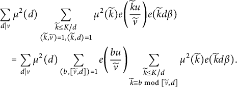
Set
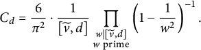
By partial summation and Lemma 10.3, we have

The contribution from the error term in (10.11) to (10.10) is
$\ll _{\varepsilon } K^{\frac {1}{2}+\frac {\theta _1}{2}+\theta _2+\varepsilon }+ K^{\frac {3\theta _1}{2}+\theta _2+\varepsilon }.$
 On the other hand, by partial summation, we obtain

Therefore, putting together (10.11) and (10.12), we find that (10.10) is equal to

The sum over b is a Ramanujan sum which is
$\leq d/(\widetilde {v},d).$
 As in the proof of Lemma 6.2, we have

Finally, we note that
$C_{d} \leq [\widetilde {v},d]^{-1}$
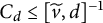 . Putting these together, we see that

We now combine (10.13) and (10.15) to arrive at our desired conclusion.
The following lemma is immediate.
Lemma 10.5 Let
$\theta _1>0$
 and
$\theta _2>0$
and
$\theta _2>0$
 be constants satisfying

Then for any
$\varepsilon>0$
 , any
$K \geq 1$
, any
$K \geq 1$
 sufficiently large in terms of
$\theta _1,\theta _2$
sufficiently large in terms of
$\theta _1,\theta _2$
 , and
$\varepsilon $
, and
$\varepsilon $
 , and any
$t \in \mathbb {R}$
, and any
$t \in \mathbb {R}$
 , and a reduced fraction
$u/v$
, and a reduced fraction
$u/v$
 such that
$1 \leq v \leq K^{\theta _1}$
such that
$1 \leq v \leq K^{\theta _1}$
 and
$\lvert t-u/v \rvert \leq K^{\theta _2-1},$
and
$\lvert t-u/v \rvert \leq K^{\theta _2-1},$
 we have

where
$\tau (v)$
 denotes the divisor function.
Proof Let
$\varepsilon>0$
 be given. For any
$\varepsilon '>0$
be given. For any
$\varepsilon '>0$
 , using Lemma 10.4 and the conditions on
$\theta _1,\theta _2$
, using Lemma 10.4 and the conditions on
$\theta _1,\theta _2$
 , we have for
$K \geq 1$
, we have for
$K \geq 1$
 sufficiently large,

Choosing
$\varepsilon '$
 sufficiently small depending on
$\theta _1,\theta _2$
sufficiently small depending on
$\theta _1,\theta _2$
 , and
$\varepsilon $
, and
$\varepsilon $
 , the proof is complete.
Following the arguments in Section 8, we can now bound the error terms by using the Erdős–Turán inequality. For each prime
$ p \in (X, 2X] $
 , we set
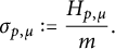
Lemma 10.6 Let
$\eta>2,A>0$
 , and
$B>0$
, and
$B>0$
 be arbitrary constants. Suppose
$X>0$
be arbitrary constants. Suppose
$X>0$
 is sufficiently large in terms of
$\eta ,A$
is sufficiently large in terms of
$\eta ,A$
 , and B, and set
$K=(\log X)^A$
, and B, and set
$K=(\log X)^A$
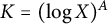 . For each prime
$p \in (X, 2X]$
. For each prime
$p \in (X, 2X]$
 , let
$f_{p,\mu }(\tau )$
, let
$f_{p,\mu }(\tau )$
 be defined by (10.2) and
$\sigma _{p,\mu }$
be defined by (10.2) and
$\sigma _{p,\mu }$
 be as in (10.16). There exists an absolute constant
$C_2>0$
be as in (10.16). There exists an absolute constant
$C_2>0$
 such that outside an exceptional set of primes
$\mathcal {E} \subseteq (X, 2X]$
such that outside an exceptional set of primes
$\mathcal {E} \subseteq (X, 2X]$
 , which depends at most on
$ X, \eta ,A$
, which depends at most on
$ X, \eta ,A$
 , and B, and satisfies

we have the uniform bounds
$H_{p, \mu } \geq \frac {1}{3} \# \{1 \leq k \leq K: \mu ^2(k)=1 \}$
 and
and

Proof The proof follows the arguments in Lemma 8.3. The only difference is that we use Lemmas 10.4 and 10.5 to obtain the bounds corresponding to Step 1 in 8.3.
The proof of Theorem 1.6 now follows from the same reasoning as in Theorem 1.1, incorporating Lemmas 10.2 and 10.6.
Acknowledgements
The authors are very grateful to the anonymous referees for their valuable suggestions that have greatly increased the clarity and value of the manuscript. The authors would also like to thank Kunjakanan Nath and Nicolas Robles for many useful comments and helpful suggestions.
Funding statement
Open access funding provided by Max Planck Society


 Open access

