


1 Introduction
Selecting predictors with a relevant effect on an outcome is fundamental in assessing a statistical model. It is particularly challenging when numerous predictors are available. Indeed, different selection strategies may lead to different results with the risk of including in the model null variables, that is, predictors with a regression coefficient equal to 0 in the true model or, on the opposite, excluding non-null variables.
This issue is encountered in many contexts, including education, where large-scale assessment data are routinely collected to measure students’ proficiency levels. In Italy, the National Institute for the Evaluation of the Education and Training System (INVALSI, https://www.invalsiopen.it/) administers standardized tests to assess students’ abilities in Italian, Mathematics, and English across grades from primary school to the end of high school. INVALSI collects many variables on students and their families. Some variables, such as parents’ education, have been widely recognized as determinants of student achievement. In contrast, other variables are just proxies and should be included in the model only if they are predictive of the outcome (e.g., the number of books at home or the availability of a room for studying). It is therefore essential to employ effective variable selection methods. The challenge is to apply those methods in this setting where most of the variables are affected by missing values, with rates as high as 26%.
Many methods for variable selection in regression models have been proposed in the literature, ranging from the classical forward, backward, and stepwise selection to modern regularization approaches, such as the lasso (Tibshirani, Reference Tibshirani1996) and the knockoff filter. The knockoffs framework (Barber & Candès, Reference Barber and Candès2015) is based on the general idea of randomly generating variables (i.e., knockoffs) that mimic the original predictors in terms of distributive properties, but are conditionally independent of the response variable given the original variables. Then, the importance of these copies is compared with that of the original variables using a suitable statistic based on the corresponding regression coefficients. As any other selection method, the knockoff filter aims at identifying the relevant (i.e., non-null) variables, but it has the peculiarity of controlling for the false discovery rate (FDR), that is, the expected proportion of false discoveries (i.e., null variables wrongly declared as non-null) or, alternatively, the expected number of false discoveries, that is, the per family error rate (PFER). We stress that controlling FDR (or PFER) is particularly important in high-dimensional settings, where the large number of available predictors poses a severe risk of selecting non-relevant (i.e., null) variables.
Numerous contributions have followed in the knockoff literature within a few years. However, even if the theory underlying the knockoffs is valid for any joint distribution of the predictors, traditional methods for generating knockoffs are limited to continuous predictors, specifically multivariate normal distributions; furthermore, they require complete data. Therefore, they are not fully appropriate in many real-world applications. A recent extension to treat mixed types of variables is due to Kormaksson et al. (Reference Kormaksson, Kelly, Zhu, Haemmerle, Pricop and Ohlssen2021), which, however, still requires complete data. To our knowledge, the only approach that handles both categorical predictors and missing values is the one proposed by Xie et al. (Reference Xie, Chen, von Davier and Weng2023). These authors consider missing values depending only on non-null variables, according to the assumption of strong missing at random (SMAR), which is more restrictive than the standard missing at random (MAR; Little & Rubin, Reference Little and Rubin2002). Their approach relies on a latent variable model in which the predictors are assumed to follow a multivariate normal distribution, which is then categorized to handle binary and ordinal observed variables. The latent variable model is estimated through maximum likelihood, and the missing values are integrated out via an expectation–maximization (EM) algorithm (Dempster et al., Reference Dempster, Laird and Rubin1977). In summary, even if Xie et al. (Reference Xie, Chen, von Davier and Weng2023) specify a complex model, their approach relies on restrictive assumptions about both the missingness mechanism and the type of predictors. In particular, their approach can handle only continuous and binary/ordered predictors, a limitation in settings with unordered categorical predictors, such as the INVALSI data. Note that an unordered predictor with K levels can be represented by a set of
$K-1$
 binary variables. However, the method of Xie et al. (Reference Xie, Chen, von Davier and Weng2023)—as well as the standard lasso—treats these dummy variables as independent predictors, so that some may be selected and others not, depending on the arbitrary choice of the reference category (Huang et al., Reference Huang, Tibbe, Tang and Montoya2024). This approach conflates two distinct problems: deciding whether a predictor should be included in the model, and determining whether some of its categories should be collapsed. In our view, these are conceptually different steps. In the variable selection phase, the primary goal is to assess the relevance of the predictor as a whole, whereas decisions about collapsing categories should be addressed only after establishing that the variable is relevant.
To overcome the mentioned limitations, we propose to embed the knockoffs method into a multiple imputation (MI; Rubin, Reference Rubin1987, Reference Rubin1996) framework, separating the phase of treatment of missing data from the phase of variable selection. MI is a general and well-established approach to handling missing values under an MAR mechanism. Since MI produces a set of complete datasets, applying any standard variable selection method to each imputed dataset is straightforward. The challenge is to decide how to combine the results from the imputed datasets. In fact, the results can be combined with Rubin’s rules for inference on model parameters, ensuring well-defined properties. However, for variable selection methods, there are no theoretical results on the properties of the combined results (see Grilli et al., Reference Grilli, Marino, Paccagnella and Rampichini2022, and the references therein). Therefore, the choice should be guided by evidence from simulation studies.
The rest of the article is organized as follows. Section 2 illustrates the proposed knockoffs method with MI. Section 3 summarizes the results of a simulation study to assess the performance of the new method compared with the approach of Xie et al. (Reference Xie, Chen, von Davier and Weng2023). Section 4 describes the INVALSI large-scale assessment data and reports the results of the analysis based on the proposed method. Section 5 offers some final remarks. Finally, Appendix A reports the results of a data-driven simulation study tailored to an INVALSI-type setting.
2 Variable selection via knockoffs in the presence of missing values
In this section, we review the fundamentals of variable selection using the knockoff filter, starting with the original approach designed for continuous variables, then outlining a sequential knockoffs method that also properly handles categorical variables. Then, we illustrate our proposal to exploit MI to implement the knockoff filter in the presence of missing values.
2.1 The knockoff filter: Methodological background
The knockoff filter has a very recent history among methods for selecting the set of non-null variables, namely, the predictors that affect the outcome in the population model. Its introduction dates back to the work of Barber and Candès (Reference Barber and Candès2015), then extended by Candès et al. (Reference Candès, Fan, Janson and Lv2018). Unlike traditional variable selection methods (e.g., stepwise selection and lasso), the knockoff filter explicitly controls the PFER or FDR. Let
$S_D$
 be the set of discoveries (i.e., selected variables), and
$S_F$
be the set of discoveries (i.e., selected variables), and
$S_F$
 be the set of false discoveries (i.e., selected variables with a null effect), then

and

Given a regression model for the outcome Y on the observed p predictors
$\mathbf X=[X_1, \ldots , X_p]$
 , the knockoffs
$\tilde {\mathbf X}=[\tilde {X}_1, \ldots , \tilde {X}_p]$
, the knockoffs
$\tilde {\mathbf X}=[\tilde {X}_1, \ldots , \tilde {X}_p]$
 are randomly generated variables independent of Y conditionally on
$\mathbf X$
are randomly generated variables independent of Y conditionally on
$\mathbf X$
 and with the following swapping property, holding for any subset S of predictors:

where
$S \subseteq \{1, \ldots , p\}$
 and
$\overset {d}{=}$
and
$\overset {d}{=}$
 denotes the equality in distribution. The vector
$[\mathbf X, \tilde {\mathbf X}]_{swap(S)}$
denotes the equality in distribution. The vector
$[\mathbf X, \tilde {\mathbf X}]_{swap(S)}$
 is obtained by swapping the entries
$X_j$
is obtained by swapping the entries
$X_j$
 and
$\tilde {X}_j$
and
$\tilde {X}_j$
 for any
$j \in S \subseteq \{1, \ldots , p\}$
for any
$j \in S \subseteq \{1, \ldots , p\}$
 , that is, the distribution of the augmented vector
$[\mathbf X, \tilde {\mathbf X}]$
, that is, the distribution of the augmented vector
$[\mathbf X, \tilde {\mathbf X}]$
 does not change if the original variables are swapped with the corresponding knockoff copies.
To carry out variable selection, the outcome Y is regressed on the augmented vector of predictors
$[\mathbf X, \tilde {\mathbf X}]$
 using a regularization procedure such as the lasso. Then, for each element
$X_j$
using a regularization procedure such as the lasso. Then, for each element
$X_j$
 in
$\mathbf X$
in
$\mathbf X$
 , a statistic
$W_j$
, a statistic
$W_j$
 is computed, satisfying the flip-sign property, saying that swapping the jth variable with its knockoff copy has the effect of changing the sign of
$W_j$
is computed, satisfying the flip-sign property, saying that swapping the jth variable with its knockoff copy has the effect of changing the sign of
$W_j$
 (Barber & Candès, Reference Barber and Candès2015). A commonly used statistic
$W_j$
(Barber & Candès, Reference Barber and Candès2015). A commonly used statistic
$W_j$
 is the difference between the absolute values of the estimated regression coefficients
$\hat {\hspace{-2pt}\beta}_j$
is the difference between the absolute values of the estimated regression coefficients
$\hat {\hspace{-2pt}\beta}_j$
 and
$\hat {\tilde {\hspace{-2pt}\beta }}_j$
and
$\hat {\tilde {\hspace{-2pt}\beta }}_j$
 for
$X_j$
for
$X_j$
 and its knockoff copy
$\tilde {X}_j$
and its knockoff copy
$\tilde {X}_j$
 , respectively,

The larger the value of
$W_j$
 , the stronger the evidence in favor of the relevance of
$ X_j$
, the stronger the evidence in favor of the relevance of
$ X_j$
 . Specifically, the variable
$X_j$
. Specifically, the variable
$X_j$
 is selected if
$W_j>\tau $
is selected if
$W_j>\tau $
 , where
$\tau $
, where
$\tau $
 is a constant chosen to ensure that the PFER or the FDR is not greater than the desired level (see Candès et al., Reference Candès, Fan, Janson and Lv2018, Equation (3.9)).
Since the set of selected variables according to the original knockoffs approach may depend on the specific values randomly generated for the knockoffs
$\tilde {\mathbf X}$
 , in the derandomized knockoffs approach (Ren et al., Reference Ren, Wei and Candès2023), the non-uniqueness of the knockoff solution is addressed by repeating the described procedure a given number of times. Then, variables chosen in at least a given proportion of cases are selected. Usually, a threshold equal to
$0.50$
, in the derandomized knockoffs approach (Ren et al., Reference Ren, Wei and Candès2023), the non-uniqueness of the knockoff solution is addressed by repeating the described procedure a given number of times. Then, variables chosen in at least a given proportion of cases are selected. Usually, a threshold equal to
$0.50$
 is used over
$31$
is used over
$31$
 replications.
The cited knockoff methods implicitly assume continuous predictors. To broaden the applicability of the knockoffs filter approach, Kormaksson et al. (Reference Kormaksson, Kelly, Zhu, Haemmerle, Pricop and Ohlssen2021) proposed an algorithm that handles both continuous and categorical variables. The proposed sequential knockoff method differs in the way knockoffs are generated. Specifically, the knockoff
$\tilde {X}_j$
 is randomly sampled from a normal distribution when
$X_j$
is randomly sampled from a normal distribution when
$X_j$
 is a continuous variable and from a multinomial distribution when
$X_j$
is a continuous variable and from a multinomial distribution when
$X_j$
 is a categorical variable. The characteristic parameters of these distributions (i.e., mean and variance in the normal case and vector of probabilities in the multinomial case) are estimated through a sequential procedure: for
$j=1, \ldots , p$
is a categorical variable. The characteristic parameters of these distributions (i.e., mean and variance in the normal case and vector of probabilities in the multinomial case) are estimated through a sequential procedure: for
$j=1, \ldots , p$
 , the predictor
$X_j$
, the predictor
$X_j$
 is regressed on the remaining predictors
$\mathbf {X}_{-j}$
is regressed on the remaining predictors
$\mathbf {X}_{-j}$
 and on the knockoffs generated in the previous steps
$[\tilde {X}_1, \ldots , \tilde {X}_{j-1}]$
and on the knockoffs generated in the previous steps
$[\tilde {X}_1, \ldots , \tilde {X}_{j-1}]$
 . The model for knockoff generation is a penalized linear model when
$X_j$
. The model for knockoff generation is a penalized linear model when
$X_j$
 is continuous and a penalized multinomial logit model when
$X_j$
is continuous and a penalized multinomial logit model when
$X_j$
 is categorical.
After the generation of knockoffs, the comparison among regression coefficients
$\hat {\hspace{-2pt}\beta }_j$
 and
$\hat {\tilde {\hspace{-2pt}\beta }}_j$
and
$\hat {\tilde {\hspace{-2pt}\beta }}_j$
 proceeds along the same lines as Candès et al. (Reference Candès, Fan, Janson and Lv2018), with multiple knockoffs generation and, consequently, multiple selections as in Ren et al. (Reference Ren, Wei and Candès2023).
It is worth noting that when a categorical variable with K levels is used as a predictor, it is represented in the model by
$K-1$
 dummy variables. The standard lasso treats those dummy variables as distinct predictors, so it may happen that only some of them are selected, depending on the arbitrary choice of the reference category. To avoid this issue, one can rely on a grouped lasso (Yuan & Lin, Reference Yuan and Lin2006) that treats the set of dummies as a whole. Under grouped lasso, the statistic
$W_j$
dummy variables. The standard lasso treats those dummy variables as distinct predictors, so it may happen that only some of them are selected, depending on the arbitrary choice of the reference category. To avoid this issue, one can rely on a grouped lasso (Yuan & Lin, Reference Yuan and Lin2006) that treats the set of dummies as a whole. Under grouped lasso, the statistic
$W_j$
 in (4) modifies as follows:

where
$\hat {\hspace{-2pt}\beta }_{jk}$
 and
$\hat {\tilde {\hspace{-2pt}\beta }}_{jk}$
and
$\hat {\tilde {\hspace{-2pt}\beta }}_{jk}$
 are the estimated regression coefficients of the dummy for category k (
$k = 2, \ldots , K$
are the estimated regression coefficients of the dummy for category k (
$k = 2, \ldots , K$
 ) of variable j and its knockoff copy, respectively. Other approaches to handling grouped variables in the knockoffs framework are described in Dai and Barber (Reference Dai, Barber, Balcan and Weinberger2016) and Katsevich and Sabatti (Reference Katsevich and Sabatti2019), though they consider only continuous variables.
The sequential knockoffs procedure was recently optimized computationally by Zimmermann et al. (Reference Zimmermann, Baillie, Kormaksson, Ohlssen and Sechidis2024) through the development of the sparse sequential knockoff algorithm, which introduces a preliminary phase to pre-select predictors. This phase relies on the graphical lasso (Friedman et al., Reference Friedman, Hastie and Tibshirani2008) to estimate the precision matrix of the original set of predictors. Zero entries in the precision matrix are used to identify predictors that are conditionally independent of each variable
$X_j$
 , and these predictors do not enter in the subsequent step of generating
$\tilde {X}_j$
, and these predictors do not enter in the subsequent step of generating
$\tilde {X}_j$
 . Since the graphical lasso is designed for continuous variables, Zimmermann et al. (Reference Zimmermann, Baillie, Kormaksson, Ohlssen and Sechidis2024) address the issue of categorical variables by employing a dummy encoding scheme. In this approach, conditional dependence between two categorical variables is assumed if at least one non-zero element appears in the precision matrix of the dummy-encoded representation.
All the methods described so far require complete datasets. To overcome this limitation, Xie et al. (Reference Xie, Chen, von Davier and Weng2023) proposed a general setting that extends the derandomized approach of Ren et al. (Reference Ren, Wei and Candès2023), allowing for the accommodation of both missing values and observed variables of mixed type (continuous, binary, and ordered). Their proposal relies on a restrictive version of the MAR assumption (Little & Rubin, Reference Little and Rubin2002), known as SMAR, according to which the probability of missingness depends only on non-null variables. To accommodate continuous, binary, and ordinal variables in a single model, the approach exploits a latent variable model in which the predictors are assumed to be jointly distributed as an underlying multivariate normal distribution. This model is estimated by maximum likelihood, integrating out missing values via an EM algorithm (Dempster et al., Reference Dempster, Laird and Rubin1977). Currently, the approach does not allow for unordered categorical and count variables or less restrictive assumptions about missingness. This approach, which simultaneously specifies a model for the outcome and integrates out missing data via the EM algorithm, is very efficient when the underlying assumptions hold, but is difficult to extend to other settings.
2.2 Implementing the knockoff filter with multiple imputation
To extend the range of possible models and enable flexible handling of missing data, we propose a multi-step procedure for variable selection using knockoffs, based on the following steps:
-
(i) MI of the missing data;
-
(ii) application of the knockoff filter to each imputed dataset;
-
(iii) identification of a unified set of selected variables.
Once the variable selection process is concluded, the model of interest can be fitted on the imputed datasets using the selected variables.
The first step of the proposed procedure consists of imputing missing values through MI (Rubin, Reference Rubin1987, Reference Rubin1996), a general and well-established approach to handling missing values under an MAR mechanism. Implementing the MI procedure involves several critical choices. Among these, the selection of the imputation method and the number of imputed datasets are crucial. We adopt MI by chained equations (MICE; van Buuren, Reference van Buuren2018; van Buuren & Groothuis-Oudshoorn, Reference van Buuren and Groothuis-Oudshoorn2011), a widely used and flexible approach that accommodates various types of variables and complex relationships among them. MICE is particularly advantageous in settings with both categorical and continuous variables, as it sequentially imputes missing values for each variable conditional on all others, using tailored imputation models. This flexibility makes MICE suitable for INVALSI data, characterized by a set of ordered and unordered categorical variables with varying degrees of missingness.
Another critical decision concerns the number of imputed datasets. A small number of imputed datasets, say 5, is often enough to appropriately account for the uncertainty introduced by the imputation process. However, the optimal number of imputed datasets depends on various factors, including the proportion of missing data, the mechanism underlying the missingness, and the desired precision of estimates (Graham et al., Reference Graham, Olchowski and Gilreath2007). The search for the optimal number of imputed datasets is beyond the scope of this article. In the simulation studies of Section 3 and Appendix A and in the application of Section 4, we use 10 imputed datasets to get a balance between computational burden and efficiency (Bodner, Reference Bodner2008; White et al., Reference White, Royston and Wood2011).
After imputing the missing values using MI, variable selection is performed separately for each imputed dataset using the knockoff approach. It is important to note that any knockoff method can be applied. In the simulation study of Section 3, we compare the performance of the proposed MI-based procedure using two types of knockoffs: (i) the knockoffs procedure of Ren et al. (Reference Ren, Wei and Candès2023) that is the one embedded within the algorithm of Xie et al. (Reference Xie, Chen, von Davier and Weng2023), enabling a comparison with our proposed method, under the same conditions and (ii) the sequential knockoffs procedure of Kormaksson et al. (Reference Kormaksson, Kelly, Zhu, Haemmerle, Pricop and Ohlssen2021) and Zimmermann et al. (Reference Zimmermann, Baillie, Kormaksson, Ohlssen and Sechidis2024) that properly handles categorical variables, making it particularly suitable for application to INVALSI data.
The knockoffs-based variable selection is applied to each imputed dataset separately. In this way, the FDR is controlled within each imputed dataset, but there is no guarantee to control the overall FDR. Each variable can be selected in all imputed datasets, in none, or in a proportion of them. Thus, the third step involves choosing the selection proportion, namely, the minimal proportion for a variable to be ultimately selected. A higher selection proportion reduces the probability that a variable is ultimately selected, thereby decreasing the expected number of false discoveries (i.e., non-null variables wrongly selected) and, thus, the overall FDR. Thus, a conservative choice would be to set the minimal proportion to 1, that is, ultimately select only variables selected in all the imputed datasets. However, this choice could lead to a final FDR much lower than the target one at the cost of a reduction of the ability of the procedure to correctly identify non-null variables, leading to a potentially low true positive rate (TPR):

where
$S^* \subseteq \{1, \ldots , p\}$
 is the subset of the true non-null predictors.
In the context of variable selection via stepwise, Wood et al. (Reference Wood, White and Royston2008) suggest the “majority rule,” that is, selecting a variable whenever it is chosen in the majority of the imputed datasets. However, their study does not investigate the impact of this strategy on the overall FDR. As there are no theoretical guidelines for determining the optimal selection proportion, in the simulation study presented in the next section, we examine results for different selection proportions.
3 Simulation study: Alternative methods for variable selection with missing values
We perform a Monte Carlo simulation study to investigate the properties of our proposal to embed the knockoffs method into an MI procedure. The main features of the simulation study are reported in Table 1.
Overview of the simulation study

Table 1 Long description
The table is organized into seven main categories.
1. Selection methods: Includes X C D W (Maximum likelihood with E M), M I-lasso (M I C E plus grouped lasso), M I-R W C (M I C E plus derandomized knockoffs), and M I-seq (M I C E plus sparse sequential knockoffs).
2. Tuning parameters: P F E R equals 2 (except for M I-lasso which uses minimum B I C) and 31 runs with a selection threshold of 0.5.
3. Sample size: 1,000 observations.
4. Variables: 100 total (50 binary and 50 continuous) divided into five blocks of 20. There are 10 non-null variables (5 binary and 5 continuous).
5. Missing data mechanism: S M A R (missingness depending on non-null observed variables) and M A R (missingness depending on both non-null and null observed variables).
6. Rate of missing values: 0 percent (complete data), 10 percent, 25 percent, 32 percent, and 45 percent.
7. Number of imputed datasets: 10 (not applicable to X C D W).
8. Monte Carlo replications: 100 runs.
We implement the MI-based knockoff approach using both the derandomized knockoff filter proposed by Ren et al. (Reference Ren, Wei and Candès2023) (called MI-RWC) and the sparse sequential knockoff filter introduced by Zimmermann et al. (Reference Zimmermann, Baillie, Kormaksson, Ohlssen and Sechidis2024) (called MI-seq). It is worth noting that the selection procedure is nested in both cases. First, the multiple repetition of the knockoff process (31 runs) selects the variables within each of the 10 imputed datasets, adopting a selection threshold equal to 0.5, as suggested in the literature (see, for instance, Ren et al., Reference Ren, Wei and Candès2023). Then, these selections are combined across the imputed datasets according to a given selection proportion to obtain a unique set of selected variables. In the following, we explore how the performance of the approach changes with the selection proportion.
The results obtained by these MI-based knockoff methods (i.e., MI-RWC and MI-seq) are compared with those obtained using the approach of Xie et al. (Reference Xie, Chen, von Davier and Weng2023), here called XCDW, which is currently the only well-established method for handling knockoffs with missing data. To this end, we devise a simulation study closest to that of Xie et al. (Reference Xie, Chen, von Davier and Weng2023), starting from their scripts.
To make the three approaches comparable, we set the nominal value of PFER defined in Equation (1), which is the only metric that all three approaches can control. For details on how the algorithms control PFER, see the specific references (Kormaksson et al., Reference Kormaksson, Kelly, Zhu, Haemmerle, Pricop and Ohlssen2021; Ren et al., Reference Ren, Wei and Candès2023; Xie et al., Reference Xie, Chen, von Davier and Weng2023).
In the simulation study, we also apply a standard selection procedure based on the lasso (without a knockoff filter) to the imputed datasets, denoted as MI-lasso.
The simulated scenario consists of 50 binary variables, 5 of which are non-null, and 50 continuous variables, 5 of which are non-null. The correlation structure is specified as in Xie et al. (Reference Xie, Chen, von Davier and Weng2023). In detail, the 100 variables are equally divided into five blocks (each block contains 10 binary variables and 10 continuous variables). The correlation within each block is: 0.60 for the first, second, and third blocks, and 0.30 for the fourth and fifth blocks; the correlation between pairs of blocks ranges from 0.10 to 0.30. For further details, see Xie et al. (Reference Xie, Chen, von Davier and Weng2023, Section 5, Figure 4). The response variable is generated by a linear regression model with normal errors and coefficients for non-null variables equal to
$+0.5$
 for binary variables and
$-0.5$
for binary variables and
$-0.5$
 for continuous variables.
After response generation, missing values on predictors are generated using the SMAR mechanism (as described in Xie et al., Reference Xie, Chen, von Davier and Weng2023), where missingness depends solely on non-null observed variables associated with the outcome. Specifically, in the simulation scheme of Xie et al. (Reference Xie, Chen, von Davier and Weng2023), for each individual i, 2 of the 10 non-null variables, say
$X_{ij_1}$
 and
$X_{ij_2}$
and
$X_{ij_2}$
 , are assumed to be observed and affect the probability of missing value of the remaining 98 ones, as follows:

where h is a constant that drives the rate of missing values.
Additionally, since MI is valid under the more general MAR assumption, we also consider an MAR scenario by allowing missingness on predictors to depend on two null observed variables, say
$X_{ij_3}$
 and
$X_{ij_4}$
and
$X_{ij_4}$
 , in addition to the two non-null ones. Formula (7) modifies accordingly:

Setting
$h = -1$
 in formulas (7) and (8) as in Xie et al. (Reference Xie, Chen, von Davier and Weng2023), the resulting rate of missing values in the simulations is approximately 32%. In the following, we present the results obtained adopting
$h = -2.4, -1.4, -1.0, -0.4$
in formulas (7) and (8) as in Xie et al. (Reference Xie, Chen, von Davier and Weng2023), the resulting rate of missing values in the simulations is approximately 32%. In the following, we present the results obtained adopting
$h = -2.4, -1.4, -1.0, -0.4$
 corresponding to about 10%, 25%, 32%, and 45% of missing values, respectively (Section 3.1). Then, we provide further insights focusing on the scenario with
$h = -1$
corresponding to about 10%, 25%, 32%, and 45% of missing values, respectively (Section 3.1). Then, we provide further insights focusing on the scenario with
$h = -1$
 (Section 3.2).
The simulation results are summarized by the following indices, where “discoveries” stands for “selected variables” and MC for Monte Carlo mean:

The three indices
$\widehat {PFER}$
 ,
$\widehat {FDR}$
,
$\widehat {FDR}$
 , and
$\widehat {TPR}$
, and
$\widehat {TPR}$
 represent the empirical counterparts of the theoretical ones, defined in Equations (1), (2), and (6).
3.1 Results of Monte Carlo simulations for varying rates of missing values
We start performing a preliminary check for the robustness of the proposed knockoffs methods in the absence of missing values (i.e., with complete data), within the proposed simulation scenario. Indeed, as widely documented in the literature, we expect that both derandomized knockoffs and sparse sequential knockoffs show a satisfactorily behavior. In this setting and with a nominal PFER set to 2, both derandomized and sequential knockoff filters effectively control the PFER, yielding empirical values of 1.37 and 1.51, respectively (FDR: 0.11 and 0.12; TPR: 0.99 and 1.00).
Then, we investigate the performance of MI-based approaches compared to XCDW and MI-lasso under varying rates of missing data. Table 2 reports the values of empirical PFER, FDR, and TPR under MAR for increasing rates of missing values: 10%, 25%, 32%, and 45%, generated according to Equations (7) and (8). Results under SMAR (not shown for the sake of parsimony) are similar. Note that for MI-based approaches (i.e., MI-lasso, MI-RWC, and MI-seq), performance is evaluated for different selection proportions over the 10 imputed datasets.
Simulation study: variable selection using XCDW, MI-lasso, MI-RWC, and MI-seq, for increasing rates of missing values (about 10%, 25%, 32%, and 45%), by selection proportion (MAR assumption; nominal PFER=2)

Table 2 Long description
The table is structured with a primary header row defining three main metrics: P F E R hat, F D R hat, and T P R hat. Under each metric, there are four sub-columns representing missing value rates of 10%, 25%, 32%, and 45%.
Data is organized into sections based on selection proportions:
* X C D W Method: At 10% missing values, P F E R is 0.11, F D R is 0.00, and T P R is 0.91. At 45%, P F E R rises to 56.53, F D R to 0.86, and T P R to 0.93.
* Selection proportion greater than or equal to 0.6:
- M I-lasso: P F E R ranges from 14.07 to 80.58; T P R remains high at 0.99 to 1.00.
- M I-R W C: P F E R ranges from 2.09 to 79.56.
- M I-seq: P F E R ranges from 2.18 to 12.62; T P R drops from 0.99 to 0.82.
* Selection proportion greater than or equal to 0.7:
- M I-lasso: P F E R ranges from 11.60 to 70.96.
- M I-R W C: P F E R ranges from 1.61 to 68.55.
- M I-seq: P F E R ranges from 1.65 to 7.44.
* Selection proportion greater than or equal to 0.8:
- M I-lasso: P F E R ranges from 9.41 to 56.25.
- M I-R W C: P F E R ranges from 1.19 to 51.46.
- M I-seq: P F E R ranges from 1.21 to 4.04.
* Selection proportion greater than or equal to 0.9:
- M I-lasso: P F E R ranges from 7.03 to 37.39.
- M I-R W C: P F E R ranges from 0.82 to 31.81.
- M I-seq: P F E R ranges from 0.84 to 2.00.
* Selection proportion of 1.0:
- M I-lasso: P F E R ranges from 4.91 to 16.38.
- M I-R W C: P F E R ranges from 0.48 to 12.11.
- M I-seq: P F E R ranges from 0.47 to 0.59.
Values in italics indicate an empirical P F E R less than or equal to 2.
Note: Monte Carlo means of empirical PFER (in italic if
$\leq 2$
 ), FDR, and TPR.
The simulation results highlight several key patterns. Overall, as expected, the performance of all compared methods deteriorates as the proportion of missing data increases. When the amount of missing data is low, the XCDW performs exceptionally well, while the two MI-based knockoff approaches yield comparable results.
However, when missing values increase, a clear performance gap emerges between MI-RWC and MI-seq, with the latter showing a noticeable advantage. For instance, at 32% missing values, MI-RWC never controls the PFER, even when the selection proportion equals 1 (empirical PFER settles at 2.39). In contrast, the MI-seq ensures an empirical PFER below 2 (i.e., 1.67) with a selection proportion of 0.9. In this scenario, the difference between XCDW and MI-seq also tends to diminish.
At the highest level of missing data considered (45%), the only method that still manages to control the PFER is the MI-seq—provided a high selection proportion (i.e.,
$\geq 0.9$
 ) is used—although this comes at the cost of a considerable drop in TPR, reaching a value of 0.65. On the other hand, with such high missing value rates, XCDW performs worse than the MI-based knockoff procedures, with an empirical PFER of 56.53.
These findings suggest that the optimal selection proportion for MI-based knockoff procedures is strongly influenced by the extent of missing data: the higher the proportion of missing values, the more stringent the selection rule must be. In general, the commonly recommended majority rule for MI (as suggested, for instance, by Wood et al., Reference Wood, White and Royston2008) appears insufficient in our setting. Namely, in our simulation framework, the majority rule corresponds to a selection proportion of at least
$0.6$
 , which does not adequately control the error rate under medium–high levels of missingness.
3.2 More results on simulations with 32% of missing values
Here, we focus on a specific percentage of missing values in order to further explore the performance of the various approaches under study. Specifically, we refer to simulated data with approximately 32% of missing values (
$h = -1$
 in Equations (7) and (8)) to facilitate a direct comparison with our benchmark approach (i.e., XCDW). Table 3 reports the values of the empirical PFER, FDR, and TPR and their standard deviations for the considered methods, under SMAR and MAR assumptions.
Simulation study with 32% missing values: variable selection using XCDW, MI-lasso, MI-RWC, and MI-seq, for increasing selection proportion (nominal PFER = 2)

Table 3 Long description
The table is structured with columns for Method, Missing mechanism (S M A R and M A R), and three performance metrics: P F E R hat, F D R hat, and T P R hat, each with Mean and S D (standard deviation) sub-columns.
Key data points include:
* X C D W method: For S M A R, P F E R mean is 2.12. For M A R, P F E R mean is 2.51.
* Selection proportion greater than or equal to 0.6: M I-lasso shows high P F E R (24.04 for S M A R) and high T P R (1.00). M I-seq shows lower P F E R (6.07 for S M A R) and T P R (0.94).
* Selection proportion greater than or equal to 0.7: M I-lasso P F E R decreases to 17.30 (S M A R). M I-seq P F E R decreases to 3.93 (S M A R).
* Selection proportion greater than or equal to 0.8: M I-lasso P F E R is 12.23 (S M A R). M I-seq P F E R is 2.41 (S M A R).
* Selection proportion greater than or equal to 0.9: M I-lasso P F E R is 7.46 (S M A R). M I-seq P F E R is 1.31 (S M A R).
* Selection proportion of 1: M I-lasso P F E R is 3.87 (S M A R). M I-seq P F E R is 0.53 (S M A R).
Values for P F E R are italicized when they are less than or equal to 2, which occurs for X C D W and for M I-seq at higher selection proportions.
Note: Monte Carlo means and standard deviations of empirical PFER (in italic if
$\leq 2$
 ), FDR, and TPR.
The XCDW method has an empirical PFER of 2.12 under SMAR and 2.51 under MAR, close enough to the nominal value of 2. On the other hand, for MI-based approaches, the empirical PFER depends on the selection proportion over the imputed datasets, as already discussed in Section 3.1: specifically, for MI-RWC, the empirical PFER gets close to 2 when the selection proportion is 1, whereas for MI-seq, the optimal selection proportion is between 0.8 and 0.9. The MI-lasso yields empirical PFER values much greater than 2, even when the selection proportion is 1. This last result is expected, since the MI-lasso procedure chooses the tuning parameter by minimizing the BIC, and it does not explicitly control the PFER.
Figure 1 displays the box plots based on the quartiles for empirical FDR and empirical TPR, while Figure 2 depicts the trends for an increasing selection proportion in the mean Monte Carlo values for the two indices.
Distribution of empirical FDR (left) and empirical TPR (right) under XCDW, MI-lasso, MI-RWC, and MI-seq, for an increasing selection proportion (up to bottom panels:
$\geq 0.7$
 ,
$\geq 0.8$
,
$\geq 0.8$
 ,
$\geq 0.9$
,
$\geq 0.9$
 , and
$1$
, and
$1$
 ): box plots based on Monte Carlo values for minimum, 1st quartile, median, 3rd quartile, and maximum.

Figure 1 Long description
A multi-panel grid of eight box plots organized into four rows. Each row corresponds to a selection proportion: greater than or equal to 0.7, greater than or equal to 0.8, greater than or equal to 0.9, and equal to 1.0.
Each row contains two panels:
1. Left Panel: Empirical F D R (False Discovery Rate) on the x-axis ranging from 0.0 to 0.8.
2. Right Panel: Empirical T P R (True Positive Rate) on the x-axis ranging from 0.5 to 1.0.
The y-axis for all panels lists eight categories representing four methods under two missing data conditions: X C D W S M A R, X C D W M A R, M I-lasso S M A R, M I-lasso M A R, M I-R W C S M A R, M I-R W C M A R, M I-sequ S M A R, and M I-seq M A R.
Key Trends:
* F D R Panels: As the selection proportion increases from 0.7 to 1.0, the F D R values for M I-lasso and M I-R W C generally decrease and shift left toward lower values. X C D W maintains relatively low and stable F D R across all levels. M I-seq shows the lowest F D R at the selection proportion of 1.0.
* T P R Panels: Most methods maintain high T P R values near 0.9 or 1.0. However, as the selection proportion reaches 1.0, the T P R for M I-R W C and M I-seq shows a slight decrease in median values compared to lower selection thresholds.
* Box Plot Components: Each entry shows a shaded gray box representing the interquartile range, a thick vertical line for the median, whiskers extending to the minimum and maximum values, and open circles indicating Monte Carlo outliers.
Variable selection using XCDW, MI-lasso, MI-RWC, and MI-seq, for an increasing selection proportion for ultimately selecting the variables over the imputed datasets: Monte Carlo means of FDR (left) and TPR (right). Dashed lines for MAR and solid lines for SMAR:
$\square $
 XCDW,
$\times $
XCDW,
$\times $
 MI-lasso,
$ \circ $
MI-lasso,
$ \circ $
 MI-RWC, and
$\triangle $
MI-RWC, and
$\triangle $
 MI-seq.

Figure 2 Long description
Two side-by-side line graphs. Both share an x-axis labeled selection proportion ranging from 0.1 to 1.0. Solid lines represent S M A R and dashed lines represent M A R.
Left Panel: F D R hat. The y-axis is mean F D R from 0.1 to 1.0.
- X C D W (square marker): Horizontal lines near 0.2.
- M I-lasso (times marker): Curves downward from 0.9 to 0.3.
- M I-R W C (circle marker): Curves downward from 0.9 to 0.2.
- M I-seq (triangle marker): Curves downward from 0.85 to 0.05.
Right Panel: T P R hat. The y-axis is mean T P R from 0.80 to 1.00.
- M I-lasso (times marker): Remains near 1.00 until 0.8, then drops to 0.95.
- M I-R W C (circle marker): Gradual decline from 1.00 to 0.88.
- M I-seq (triangle marker): Steeper decline from 1.00 to 0.83.
- X C D W (square marker): Horizontal lines near 0.90.
The reference values for evaluating the performance of the MI-based approaches are those achieved by XCDW: an FDR of 0.17 under SMAR and 0.20 under MAR, and a TPR of 0.91 under SMAR and 0.90 under MAR. Notably, although the XCDW approach is valid only under SMAR (i.e., missingness depending only on non-null variables), its performance is minimally affected when applied to MAR data. Across all approaches, switching from SMAR to the more general MAR results in a modest increase in FDR, while TPR remains unchanged.
Focusing on MI-based knockoff approaches, MI-RWC shows a performance comparable to that of XCDW only when variables are retained if selected in all imputed datasets (i.e., selection proportion equal to 1). Under this condition, MI-RWC achieves a Monte Carlo mean FDR of 0.17–0.18 and a mean PFER close to 2, albeit with a slight reduction in TPR (0.88–0.89). In contrast, with a selection proportion of at least
$0.9$
 , the FDR rises to approximately 0.30, and the PFER increases to over 4, with both metrics worsening further at smaller selection proportions.
A markedly different scenario emerges when evaluating the performance of MI-seq. Specifically, when variables are retained if selected in at least 0.8 of the imputed datasets, the FDR and TPR are very close to those achieved by XCDW. Increasing the selection proportion further reduces the FDR, but comes at the cost of a slight decrease in TPR, which declines from 0.91 (for a selection proportion
$\geq 0.8$
 ) to 0.88 (if the selection proportion is
$\geq 0.9$
) to 0.88 (if the selection proportion is
$\geq 0.9$
 ), reaching a minimum of 0.83 when variables are retained only if selected in all imputed datasets.
3.3 Remarks on simulation results
In summary, the MI-seq approach represents a valuable alternative to the XCDW method. Based on the simulation results described above, there is evidence that the selection proportion depends on the rate of missing values. For a low missing rate (approximately 10%), retaining a variable if selected in at least 0.7 of the imputed datasets is sufficient to control the PFER while maintaining high TPR values. When the missing rate increases to 25%–32%, this selection proportion rises to 0.9 (0.8 is almost sufficient with 25% of missingness), while the empirical TPR remains high (0.94 with 25% of missingness and 0.88 with 32% of missingness). For very high missing rates (around 45%), the general recommendation is to retain variables selected in at least 0.9 of the imputed datasets; however, this comes at the cost of a substantial reduction in TPR.
It is worth noting that the simulation design used here is the one proposed by Xie et al. (Reference Xie, Chen, von Davier and Weng2023) to validate their method. In particular, the continuous variables are assumed to be normally distributed, which is important for the XCDW method based on likelihood. Indeed, deviations from normality could negatively affect the XCDW approach. On the other hand, the normality assumption is irrelevant for the MI-based approaches, since the imputation phase for continuous variables exploits least-squares linear models. Moreover, the simulation study considers only binary and continuous variables, neglecting ordered and unordered categorical variables. Ordinal variables are admitted in XCDW, even if the selection procedure should be adapted to properly account for the ordering of categories. On the other hand, unordered categorical variables are not handled by XCDW, which is a limitation in some applications, like the INVALSI case on math test scores presented in the next section.
In order to evaluate the performance of the proposed MI-seq procedure in the INVALSI setting, which is quite different in terms of variables and missingness pattern, we conduct a further simulation study tailored to the INVALSI case. The specific simulation design and main results are illustrated in Appendix 1, showing that the MI-seq method also performs well in this setting.
4 Variable selection via knockoffs for INVALSI data on mathematics test scores
The INVALSI is the national institute that evaluates the Italian school system. Specifically, it evaluates student achievement in Mathematics, Italian, and English for different grades each year. The evaluation is based on multiple-choice questions. The selection of the set of items relies on internationally validated methods based on the Rasch model (Rasch, Reference Rasch1960), similarly to TIMSS (von Davier et al., Reference von Davier, Fishbein and Kennedy2024). The evaluation test is administered to all students across all schools to assess school performance. An additional background questionnaire is administered to students in a sample of schools to examine the relationship between achievement and students’ background characteristics. We focus on data from the INVALSI sample survey for 2022–2023 on pupils in grade 5, corresponding to the last year of primary school. The dataset includes 16,828 students nested in 501 schools.
Specifically, we consider achievement in mathematics, a latent ability measured by a set of dichotomously scored items (1: correct answer; 0: wrong answer). INVALSI provides the item response patterns and a Rasch-based estimate of ability. The average sample score in mathematics is 191.82 points, with a standard deviation of 41.07.
The dataset includes 30 student-level variables of different types:
-
- binary (e.g., gender and availability of a personal computer);
-
- ordinal (e.g., Mother’s education);
-
- unordered categorical (e.g., Mother’s occupation).
The dataset also includes the school’s geographical area, which is not included in the variable selection process because it is used as a stratification variable.
To study the relationship between background characteristics and pupils’ achievement while accounting for clustering within schools, we specify a random intercept model (Snijders & Bosker, Reference Snijders and Bosker2011). Denoting the pupils with i (level 1) and the schools with s (level 2), the model is specified as

where
$y_{is}$
 is the mathematics score of pupil i of school s,
$\mathbf {x}_{is}$
is the mathematics score of pupil i of school s,
$\mathbf {x}_{is}$
 is the vector of level 1 predictors (including the constant) with coefficients
$\boldsymbol {\beta }$
is the vector of level 1 predictors (including the constant) with coefficients
$\boldsymbol {\beta }$
 (including the intercept), and
$\mathbf {z}_{s}$
(including the intercept), and
$\mathbf {z}_{s}$
 is the vector of level 2 predictors with coefficients
$\boldsymbol {\gamma }$
is the vector of level 2 predictors with coefficients
$\boldsymbol {\gamma }$
 . The level 1 errors are assumed to be independent and identically distributed,
$e_{is} \sim N(0, \sigma _e^2)$
. The level 1 errors are assumed to be independent and identically distributed,
$e_{is} \sim N(0, \sigma _e^2)$
 , and the level 2 errors (random effects) are assumed to be independent and identically distributed,
$u_s \sim N(0, \sigma _u^2)$
, and the level 2 errors (random effects) are assumed to be independent and identically distributed,
$u_s \sim N(0, \sigma _u^2)$
 . Moreover, the errors at the two levels are assumed to be independent.
The background variables are highly correlated, and there are no theoretical guidelines for choosing among them, which calls for a data-driven selection procedure.
Moreover, a critical issue of the data is the relevant rate of missing values for many student-level variables, ranging from
$1.6$
 % to
$25.5$
% to
$25.5$
 %. Specifically, the variables with the highest rates of missing values are Father’s and Mother’s education and occupation (ranging from 23.4% to 25.5%), followed by Italian language at home, Dialect spoken at home, Italian used with friends, and Nursery school (about 10%). A complete-case analysis would halve the number of students, leading to a large loss of power and, especially, potentially high bias, given that the missing mechanism cannot be assumed to be missing completely at random. Rather, an MAR mechanism with missingness depending on observed values may be plausible, so MI is a viable approach to preserve the original sample size and avoid bias in the estimators.
To perform variable selection while handling missing data, we follow the proposed procedure described in Section 2.2, namely, MI-seq. It is worth noting that the other procedures (i.e., XCDW and MI-RWC) are not suitable, as they do not handle variables with unordered categories, such as Immigrant status, Father’s occupation, and Mother’s occupation.
The MI-seq is applied to the INVALSI case study, implementing MICE with 10 imputed datasets using the mice package of R (van Buuren & Groothuis-Oudshoorn, Reference van Buuren and Groothuis-Oudshoorn2011). Each variable is imputed with a model suitable for its measurement scale: logit model for binary variables, cumulative logit model for ordinal variables, and multinomial logit model for unordered categorical variables.
For each imputed dataset, the predictors are selected using the sequential knockoffs procedure of Kormaksson et al. (Reference Kormaksson, Kelly, Zhu, Haemmerle, Pricop and Ohlssen2021), as implemented in the R package knockofftools (Zimmermann et al., Reference Zimmermann, Baillie, Kormaksson, Ohlssen and Sechidis2024) with options PFER = 2 and method="sparseseq". Unordered categorical and ordinal variables are coded using a set of dummy variables with a baseline category. In the knockoffs filter, we use group lasso (Yuan & Lin, Reference Yuan and Lin2006) instead of standard lasso to prevent the selection from depending on the arbitrary choice of the baseline category. In this way, the corresponding set of dummy variables is jointly selected or discarded for each predictor. The procedure runs 31 times for each imputed dataset, and a predictor is retained if it is selected in at least 50% of the runs.
Table 4 shows the predictors with the proportion selected over the 10 imputed datasets by the sequential knockoffs procedure. A notable feature of the results is the clear separation in selection proportions: predictors are either selected in nearly all imputed datasets (selection proportion 0.9 or 1) or rarely selected (with proportions less than or equal to 0.3). This pattern indicates a high degree of stability in the selection results across the imputation process, suggesting that the contributions of most predictors are clearly identified despite missing data. Therefore, the choice of which variables to retain does not appear particularly problematic in this situation. Predictors included in the final model are denoted by a check mark in Table 4. Overall, 22 out of 30 variables have been selected.
Variable selection via MI-seq: proportion selected over 10 imputed datasets and retained status (
$\checkmark $
 if proportion
$\ge 0.8$
if proportion
$\ge 0.8$
 )
)

Table 4 Long description
The table consists of four columns: Variable, Levels, Prop. (Proportion), and Retained. A checkmark in the Retained column indicates a proportion greater than or equal to 0.8.
* Male: 1=yes, 0=no. Prop. 1. Retained with checkmark.
* No. of brothers: ordinal, 5 levels. Prop. 1. Retained with checkmark.
* No. of sisters: ordinal, 5 levels. Prop. 1. Retained with checkmark.
* At home, you have:
- quiet space: 1=yes, 0=no. Prop. 0.9. Retained with checkmark.
- computer: 1=yes, 0=no. Prop. 1. Retained with checkmark.
- personal desk: 1=yes, 0=no. Prop. 0.3. Not retained.
- software: 1=yes, 0=no. Prop. 0. Not retained.
- internet connection: 1=yes, 0=no. Prop. 1. Retained with checkmark.
- personal room: 1=yes, 0=no. Prop. 1. Retained with checkmark.
- classical books: 1=yes, 0=no. Prop. 0. Not retained.
- artworks: 1=yes, 0=no. Prop. 0. Not retained.
- technical manuals: 1=yes, 0=no. Prop. 0. Not retained.
- dictionary: 1=yes, 0=no. Prop. 1. Retained with checkmark.
- personal tablet: 1=yes, 0=no. Prop. 1. Retained with checkmark.
- smartphone: 1=yes, 0=no. Prop. 1. Retained with checkmark.
* No. of books: ordinal, 5 levels. Prop. 1. Retained with checkmark.
* Student origin and language:
- Student born in Italy: 1=yes, 0=no. Prop. 1. Retained with checkmark.
- Immigrant status: 1=native; 2=1st gen immigrant; 3=2nd gen imm. Prop. 0. Not retained.
- Italian language at home: 1=yes, 0=no. Prop. 1. Retained with checkmark.
- Dialect spoken at home: 1=yes, 0=no. Prop. 1. Retained with checkmark.
- Italian used with friends: 1=yes, 0=no. Prop. 1. Retained with checkmark.
* Parents:
- Father born in Italy: 1=yes, 0=no. Prop. 0.2. Not retained.
- Mother born in Italy: 1=yes, 0=no. Prop. 1. Retained with checkmark.
- Father’s education: 1=compulsory, 2=high sch., 3=college, 4=master plus. Prop. 1. Retained with checkmark.
- Mother’s education: 1=compulsory, 2=high sch., 3=college, 4=master plus. Prop. 1. Retained with checkmark.
- Father’s occupation: 1=unemployed, 2=manager/clerk, 3=self-employed, 4=blue collar, 5=professional, 6=housewife/retired. Prop. 1. Retained with checkmark.
- Mother’s occupation: 1=unemployed, 2=manager/clerk, 3=self-employed, 4=blue collar, 5=professional, 6=housewife/retired. Prop. 1. Retained with checkmark.
* Student career:
- Nursery school: 1=yes, 0=no. Prop. 1. Retained with checkmark.
- Regular student: 1=yes, 0=no. Prop. 1. Retained with checkmark.
- School weekly hours greater than 30: 1=yes, 0=no. Prop. 0. Not retained.
- School area: 1=N W; 2=N E; 3=Center; 4=South; 5=S-Islands. Retained by default.
Note: INVALSI grade 5 sample survey, year 2022–2023.
The sequential knockoff procedure gives parameter estimates based on the group lasso for a standard linear model, that is, without random effects. This is not a limitation for selecting the predictors, since in the linear model, there is an equivalence between the regression coefficients conditional on the random effects and the marginal ones (Ritz & Spiegelman, Reference Ritz and Spiegelman2004). Notwithstanding, we need to fit a random effect model with the selected variables for two reasons: (i) to obtain standard errors properly accounting for the school clustering and (ii) to avoid the downward bias implicit in lasso-based procedures (e.g., Belloni & Chernozhukov, Reference Belloni and Chernozhukov2013). For these reasons, we fit the random intercept model (9) with the selected predictors to each imputed dataset via maximum likelihood using the R package lme4 (Bates et al., Reference Bates, Mächler, Bolker and Walker2015). The results across the 10 imputed datasets are combined using Rubin’s rules (Rubin, Reference Rubin1987) to obtain point estimates and standard errors.
Table 5 reports the residual variances and the intraclass correlation coefficient (ICC) for the model without predictors (null model) and for the model with the predictors selected by sequential knockoffs (full model; see Table 4). The null model shows that the variability in the mathematics scores due to school clustering is
$13.8\%$
 . The predictors explain about
$23\%$
. The predictors explain about
$23\%$
 of the school-level variance and about
$15\%$
of the school-level variance and about
$15\%$
 of the pupil-level variance. Given the included predictors, the residual ICC in the final model is
$12.6\%$
of the pupil-level variance. Given the included predictors, the residual ICC in the final model is
$12.6\%$
 , indicating that school clustering remains relevant.
Random intercept null model and full model with selected predictors (Table 4): combined estimates of the residual variances based on 10 imputed datasets

Table 5 Long description
The table consists of four columns: Residual variances, Null model, Full model, and percentage Explained.
* Level 2 school: Null model is 233.30, Full model is 178.94, and percentage Explained is 23.30.
* Level 1 pupil: Null model is 1,461.94, Full model is 1,239.97, and percentage Explained is 15.18.
* Total: Null model is 1,695.24, Full model is 1,418.91, and percentage Explained is 16.30.
* I C C: Null model is 13.76 percent, Full model is 12.61 percent, and percentage Explained is blank.
A note at the bottom indicates the data is from the I N V A L S I grade 5 sample survey, year 2022 to 2023.
Note: INVALSI grade 5 sample survey, year 2022–2023.
Table 6 presents the point estimates and corresponding standard errors for the full model, obtained through Rubin’s rules. It is worth noting that the standard errors account for the variability due to MI; however, they ignore the uncertainty implicit in the variable selection process through knockoffs and, thus, are likely to be underestimated, raising a problem for post-selection inference. Although formal inference is therefore limited, the selected variables and their estimated effects still provide valuable insights into the relationship between students’ background characteristics and achievement. In particular, the direction (i.e., the sign) and relative magnitude of the regression coefficients allow for a meaningful interpretation of the main determinants of performance. This is in line with previous findings showing that knockoff-based procedures are effective in identifying the direction of the effects (Barber & Candès, Reference Barber and Candès2019) and is further supported in our data setting by the simulation results reported in Appendix 1. In the following, we therefore focus on the interpretation of the point estimates.
Random intercept model with selected predictors: combined estimates of the regression coefficients and standard errors based on 10 imputed datasets

Table 6 Long description
The table contains three columns: Variable, Estimate, and Std. error. Key data points include:
* Intercept: Estimate 124.26, Std. error 4.016.
* Male: Estimate 9.55, Std. error 0.568.
* Number of brothers (reference 0): 1 (minus 4.33, 0.652), 2 (minus 6.98, 1.082), 3 (minus 11.92, 1.961), greater than or equal to 4 (minus 12.70, 2.929).
* Number of sisters (reference 0): 1 (minus 3.00, 0.645), 2 (minus 5.38, 1.109), 3 (minus 9.55, 2.472), greater than or equal to 4 (minus 11.28, 3.776).
* Home resources: quiet space (1.20, 0.832), computer (3.39, 0.612), internet connection (4.49, 0.862), personal room (minus 2.58, 0.613), dictionary (8.47, 1.003), personal tablet (minus 4.11, 0.586), smartphone (minus 4.29, 0.661).
* Number of books (reference 0 to 10): 11 to 25 (3.96, 0.933), 26 to 100 (12.34, 0.966), 101 to 200 (15.39, 1.126), greater than 200 (17.33, 1.262).
* Student origin and language: Born in Italy (6.31, 1.673), Italian at home (4.56, 1.071), Dialect at home (minus 1.91, 0.617), Italian with friends (9.87, 1.540), Mother born in Italy (minus 1.69, 0.975).
* Father's education (reference compulsory): high school (5.31, 0.921), college (8.72, 1.541), master or more (10.49, 1.333).
* Mother's education (reference compulsory): high school (5.54, 0.885), college (6.75, 1.342), master or more (10.36, 1.316).
* Father's occupation (reference unemployed): manager/clerk (7.11, 1.857), self-employed (5.60, 1.858), blue collar (2.90, 1.828), professional (5.58, 1.922), housewife/retired (2.68, 3.546).
* Mother's occupation (reference unemployed): manager/clerk (2.11, 1.483), self-employed (1.32, 1.659), blue collar (minus 0.76, 1.522), professional (2.80, 1.637), housewife/retired (minus 0.62, 1.495).
* Student career: Nursery school (8.90, 1.520), Regular student (5.18, 2.287).
* School area (reference North-West): North-East (2.96, 2.147), Center (5.59, 2.161), South (8.65, 2.089), South-Islands (minus 1.39, 2.151).
Note: INVALSI grade 5 sample survey, year 2022–2023.
In general, the estimated effects are consistent with expectations and with the existing literature on educational achievement. For example, the gender gap in favor of males is confirmed (Contini et al., Reference Contini, Di Tommaso and Mendolia2017).
In analyses of large-scale assessment data, families’ cultural background and socioeconomic status (SES) are typically associated with an advantage in educational achievement. Our results confirm this relationship. In particular, the largest effect pertains to the number of books at home, a well-established proxy of the cultural environment (Heppt et al., Reference Heppt, Olczyk and Volodina2022). As for SES, it is often measured through an indicator that summarizes parental education and occupation (e.g., Cascella, Reference Cascella2025). Here, we keep these components separate in order to estimate their specific effects. It turns out that the effects of parental education are similar for mothers and fathers and increase monotonically from compulsory schooling to a master’s degree or higher, in line with a large body of literature documenting the role of family background in shaping educational outcomes. On the other hand, the effect of the Father’s occupation appears stronger than that of the mother, which is not statistically significant.
Other findings provide interesting additional insights. In particular, personal tablet or smartphone ownership is associated with lower mathematics scores. Since the test evaluates mathematics proficiency acquired during primary school, this result may reflect substitution effects between screen time and study-related activities or, more broadly, differences in the family environment (Beland & Murphy, Reference Beland and Murphy2016). While causal interpretations are beyond the scope of this analysis, this finding highlights potentially relevant learning mechanisms that deserve further investigation.
Finally, it is worth noting that the selected variables can be used to predict a student’s response. Indeed, the results of the data-driven simulation study presented in Appendix 1 show that models based on variables selected by the MI-seq procedure achieve predictive performance essentially indistinguishable from that obtained using the true underlying predictors. This evidence suggests that the selection procedure is not only effective at identifying relevant variables but also preserves the model’s predictive capability in realistic scenarios.
5 Final remarks
In this contribution, we analyzed the effect of student characteristics on mathematics ability in the Italian primary school. These data call for a variable selection method that handles missing values. To this aim, we proposed an approach, called MI-seq, based on knockoffs. The proposed method consists of the following sequential steps: first, missing values are addressed through MI techniques; second, for each imputed dataset, variables are selected using a knockoffs method, and only those variables selected in at least a predefined minimal proportion of datasets are retained. This multi-step structure provides substantial flexibility, distinguishing the MI-seq from the recent contribution by Xie et al. (Reference Xie, Chen, von Davier and Weng2023), called here XCDW, which, to the best of our knowledge, is the only one that applies the knockoff method in the presence of missing data. Unlike XCDW, MI-seq does not require assumptions about the distributions of continuous variables and can handle unordered categorical variables alongside continuous, binary, and ordinal variables. Moreover, MI-seq yields results valid using the standard MAR assumption instead of the more restrictive SMAR assumption of XCWD, where the missing data mechanism depends only on non-null variables. Finally, separating the imputation and modeling steps makes it straightforward to specify any kind of model, whereas, in XCWD, using a different model would require a non-trivial modification of the likelihood function and the EM algorithm.
These advantages of MI-seq are made possible because of the following features: (i) the use of MI to deal with missing values, allowing to deal with any variables under the MAR assumption and (ii) the selection of variables based on the sequential knockoffs procedure of Kormaksson et al. (Reference Kormaksson, Kelly, Zhu, Haemmerle, Pricop and Ohlssen2021) and Zimmermann et al. (Reference Zimmermann, Baillie, Kormaksson, Ohlssen and Sechidis2024) that allows to generate knockoff copies of unordered categorical variables based on the multinomial logit model, differently from standard knockoffs procedures (see, e.g., Ren et al., Reference Ren, Wei and Candès2023), which are designed for continuous variables.
To evaluate the performance of the MI-seq, we conducted a simulation study under the scenario proposed by Xie et al. (Reference Xie, Chen, von Davier and Weng2023), obtaining similar performance for a rate of missing values around 32% and better performance for a rate of 45% of missingness. Interestingly, MI-seq performed better than the approach that integrates MI with the derandomized knockoff procedure of Ren et al. (Reference Ren, Wei and Candès2023) (referred to in the text as MI-RWC), likely because half of the variables are binary in the simulation. We checked the performance of the proposed method in the context of the INVALSI case study, characterized by several unordered categorical variables affected by missing values, by means of an additional data-driven simulation study illustrated in Appendix 1. This simulation proved the validity of the proposed MI-seq method in the INVALSI scenario.
A limitation of the proposed MI-seq approach is that it does not strictly control the PFER or the FDR, contrary to knockoff filters for complete data and the XCDW method of Xie et al. (Reference Xie, Chen, von Davier and Weng2023) for SMAR data. In fact, any MI-based procedure requires choosing the minimal proportion of imputed datasets for ultimately retaining a variable, and the PFER is inversely related to this proportion. Furthermore, the simulation study shows that the minimal selection proportion required to control the PFER increases with the rate of missing values. The “majority rule” is generally inadequate even with a low missingness rate (10%), where a selection proportion of at least 0.7 is preferable. Remarkably, for higher levels of missingness, the optimal selection proportion approaches 0.9. Anyway, it is worth noting that the choice of this proportion is not always critical, as outlined by the data-driven simulation study reported in Appendix 1, since, in applications, it may happen that the selection is not very sensitive to this parameter. Remarkably, in our case study, the non-null variables were clearly identified since the actual proportions were either
$\ge 0.9$
 or
$\le 0.3$
or
$\le 0.3$
 . As a general strategy, we recommend monitoring the set of retained variables as the selection proportion decreases from
$1$
. As a general strategy, we recommend monitoring the set of retained variables as the selection proportion decreases from
$1$
 to
$0.5$
to
$0.5$
 : if the set is relatively stable, the selection is trustworthy; otherwise, it is advisable to set up a simulation study tailored on the empirical setting, like the one presented in Appendix 1.
The implementation of MI-based methods via MICE may raise computational issues in high-dimensional data. Possible solutions include dividing variables into blocks or using regularization techniques in the imputation phase (van Buuren, Reference van Buuren2018).
A further challenging issue concerns the post-selection inference in the presence of missing data. Indeed, the standard errors obtained from fitting the model with selected predictors are underestimated because they ignore the uncertainty introduced by the selection process. A general solution to this issue is data splitting, which involves randomly partitioning the data into two sets, one for variable selection and the other for model fitting and inference (see, for instance, García Rasines & Young, Reference García Rasines and Young2023; Wasserman & Roeder, Reference Wasserman and Roeder2009). In case of missing values, MI should be run on each of the two sets separately to avoid generating dependence between them.
Finally, a general issue with knockoffs, unrelated to missing data, concerns their performance in selecting cluster-level predictors in multilevel analysis. In fact, the available methods to generate the knockoffs do not account for the levels of the predictors, so a copy of a cluster-level variable is produced as if it were an individual-level variable, ignoring the constraint that it has to be constant within the clusters. This limitation does not apply in the INVALSI case study because all predictors are at the student level (except for the geographical area, which, however, is not included in the selection procedure). However, applications of multilevel models often involve many cluster-level predictors; thus, it is essential to investigate the extent to which the selection process for cluster-level predictors is negatively affected by the use of knockoffs designed for individual-level predictors and to devise effective solutions.
Supplementary material
The supplementary material for this article can be found at https://doi.org/10.1017/psy.2026.10109.
Data availability statement
The data used in the article are the property of INVALSI. In the Supplementary Material, we provide the R codes to replicate the simulation study described in Section 3 (under MAR and using the sparse sequential knockoffs method) and to select variables on INVALSI-type simulated data.
Acknowledgments
We are grateful to the National Institute for the Evaluation of the Italian School System (INVALSI), which provided the data for the case study reported in the article. INVALSI is not responsible for the analyses and data processing reported in the article. This manuscript is part of the special section, Integrating and Analyzing Complex High-Dimensional Data in Social and Behavioral Sciences Research. We extend our heartfelt gratitude to the co-Guest Editors, Drs Katrijn Van Deun and Eric Lock, as well as the reviewers for their invaluable and insightful feedback, which significantly enhanced this article.
Author contributions
All authors contributed equally to this work.
Funding statement
This work was supported by the Italian Ministry of University and Research (MUR) under grant Department of Excellence project 2023–2027 ReDS “Rethinking Data Science”—Department of Statistics, Computer Science, Applications—University of Florence (Cup B13C22004500001), and Italian Ministry of University and Research (MUR) under grant PRIN 2022 Call (D.D. 104/2022), project “Latent variable models and dimensionality reduction methods for complex data” (Project No. 20224CRB9E, CUP B53C24006320006).
Competing interests
The authors declare none.
Appendix A Data-driven simulation study based on the INVALSI data structure
To investigate the appropriateness of the MI-seq approach for addressing variable selection in the INVALSI setting, characterized by unordered categorical predictors and missing data, we present an additional simulation study specifically designed to closely mimic the INVALSI application. This simulation employs a data-driven strategy, where the joint distribution of the predictors and the missingness pattern are directly inherited from the observed INVALSI data.
Let
$\mathbf {X}$
 denote the covariate matrix from the INVALSI dataset, which includes binary, ordered, and unordered categorical predictors with multiple levels, as well as non-negligible amounts of missing data (see Table 4 for the list of variables). To sample the response variable according to a known data-generating model, we proceed as follows:
-
1. The missing values of the matrix $\mathbf {X}$
 are imputed once using MICE to get a complete matrix
$\mathbf {X}_{imp}$
.
are imputed once using MICE to get a complete matrix
$\mathbf {X}_{imp}$
. -
2. To obtain realistic effect sizes, the observed INVALSI response vector $\mathbf {y}$
is regressed on the imputed matrix
$\mathbf {X}_{imp}$
using lasso (with grouped lasso penalty for unordered categorical predictors). -
3. The vector of the lasso estimates of the regression coefficients, denoted by $\boldsymbol {\beta }_{true}$
, defines the data-generating model and is used to generate the new response vector following the linear regression model
$\mathbf {y}_{gen} = \mathbf {X}_{imp} \boldsymbol {\beta }_{true} + \boldsymbol {\varepsilon }$
, where the errors are independently sampled from a normal distribution with mean 0 and standard deviation set on the basis of the lasso residuals.


The dataset used for the simulation consists of the generated response values
$\mathbf {y}_{gen}$
 and the original covariate matrix
$\mathbf {X}$
and the original covariate matrix
$\mathbf {X}$
 (i.e., the original observed data with missing values). From this dataset,
$R = 50$
(i.e., the original observed data with missing values). From this dataset,
$R = 50$
 random subsamples of half of the
$16,828$
random subsamples of half of the
$16,828$
 observations are drawn without replacement and used as a training set, while the remaining observations form a corresponding test set. This sampling scheme substantially reduces computational costs while enabling evaluation of variable selection performance, the correctness of regression coefficients’ signs, and the out-of-sample prediction performance.
For each training set, the MI-seq procedure is applied as described in Section 2.2, that is, imputing missing covariates with MICE and selecting predictors using the sparse sequential knockoff approach. Variable selection performance is evaluated across the replications by the empirical PFER, FDR, and TPR. Table A1 reports the distributions of
$\widehat {PFER}$
 ,
$\widehat {FDR}$
,
$\widehat {FDR}$
 , and
$\widehat {TPR}$
, and
$\widehat {TPR}$
 for different selection proportions.
Data-driven simulation study—Variable selection with MI-seq, for increasing selection proportion (nominal PFER
$=2$
 ): Monte Carlo means and standard deviations of empirical PFER, FDR, and TPR

Table A1 Long description
The table consists of seven columns. The first column lists the selection proportion, followed by three pairs of columns for Mean and S D (Standard Deviation) corresponding to P F E R hat, F D R hat, and T P R hat.
* Selection proportion greater than or equal to 0.1: P F E R Mean 0.618, S D 0.850; F D R Mean 0.027, S D 0.035; T P R Mean 0.858, S D 0.055.
* Selection proportion greater than or equal to 0.2 and 0.3: P F E R Mean 0.600, S D 0.784; F D R Mean 0.027, S D 0.034; T P R Mean 0.856, S D 0.052.
* Selection proportion greater than or equal to 0.4: P F E R Mean 0.582, S D 0.738; F D R Mean 0.026, S D 0.032; T P R Mean 0.856, S D 0.052.
* Selection proportion greater than or equal to 0.5 through 0.9: P F E R Mean 0.582, S D 0.738; F D R Mean 0.026, S D 0.033; T P R Mean 0.855, S D 0.051.
* Selection proportion 1.0: P F E R Mean 0.582, S D 0.738; F D R Mean 0.026, S D 0.033; T P R Mean 0.855, S D 0.051.
Table A1 shows that the MI-seq approach works well in the proposed setting. In fact, the PFER is controlled, whereas the TPR (proportion of truly non-null variables selected) is satisfactory. Furthermore, in the particular setting at issue, the results are not influenced by the selection proportion.
To further assess the practical relevance of MI combined with knockoffs, we also evaluate the approach’s ability to correctly identify the sign of the predictors’ effects. To this end, the set of variables selected on the training data is used to fit the model on the test data.
Each test set is multiply imputed using the MICE procedure, generating 10 complete versions of the test data.
For each imputed test set, a linear regression model is fitted using the variables selected in the corresponding training set, yielding a set of estimated coefficient vectors. We set the selection proportion to 0.7, though this choice has little consequence in this application. These coefficient estimates are then combined using Rubin’s rules, resulting in a single pooled coefficient vector for each test set. By repeating this procedure on all
$R = 50$
 test sets, we obtain 50 estimates of the regression coefficients to compare with the true coefficient vector
$\boldsymbol {\beta }_{true}$
test sets, we obtain 50 estimates of the regression coefficients to compare with the true coefficient vector
$\boldsymbol {\beta }_{true}$
 .
.
To evaluate the ability of the selection method to correctly identify the sign of the regression coefficients, we classify the coefficients as negative, null, and positive, then compute the agreement between true and estimated coefficients using Cohen’s Kappa (Cohen, Reference Cohen1960). We obtain satisfactory results, as Cohen’s Kappa coefficient lies in the range
$[0.677, 0.939]$
 , with an average value of 0.808 (median of 0.820).
Furthermore, even if the primary aim of the knockoff method is selecting non-null variables, it is of interest to assess the predictive ability of the model based on the selected variables. For this aim, we first select the variables and estimate the regression coefficients on each training set; the resulting coefficients are then used to predict the outcome on the corresponding test set. The MC mean of the mean absolute error (MAE) is 8.006 and of the mean squared relative error (MSRE) is 0.003. As a benchmark, we also compute predictions using the true non-null variables, obtaining MAE = 8.001 and MSRE = 0.003. These results indicate that, in the setting considered here, the selection process based on MI-seq preserves the model’s predictive capability.
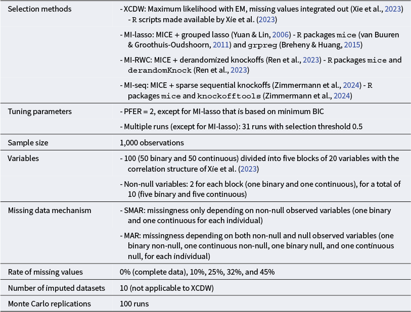
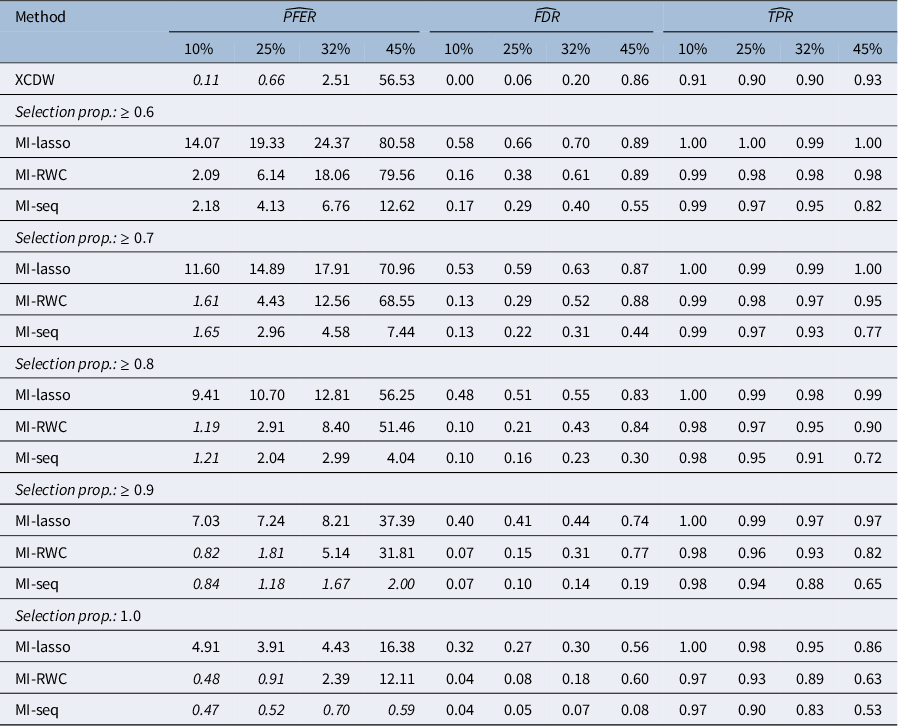
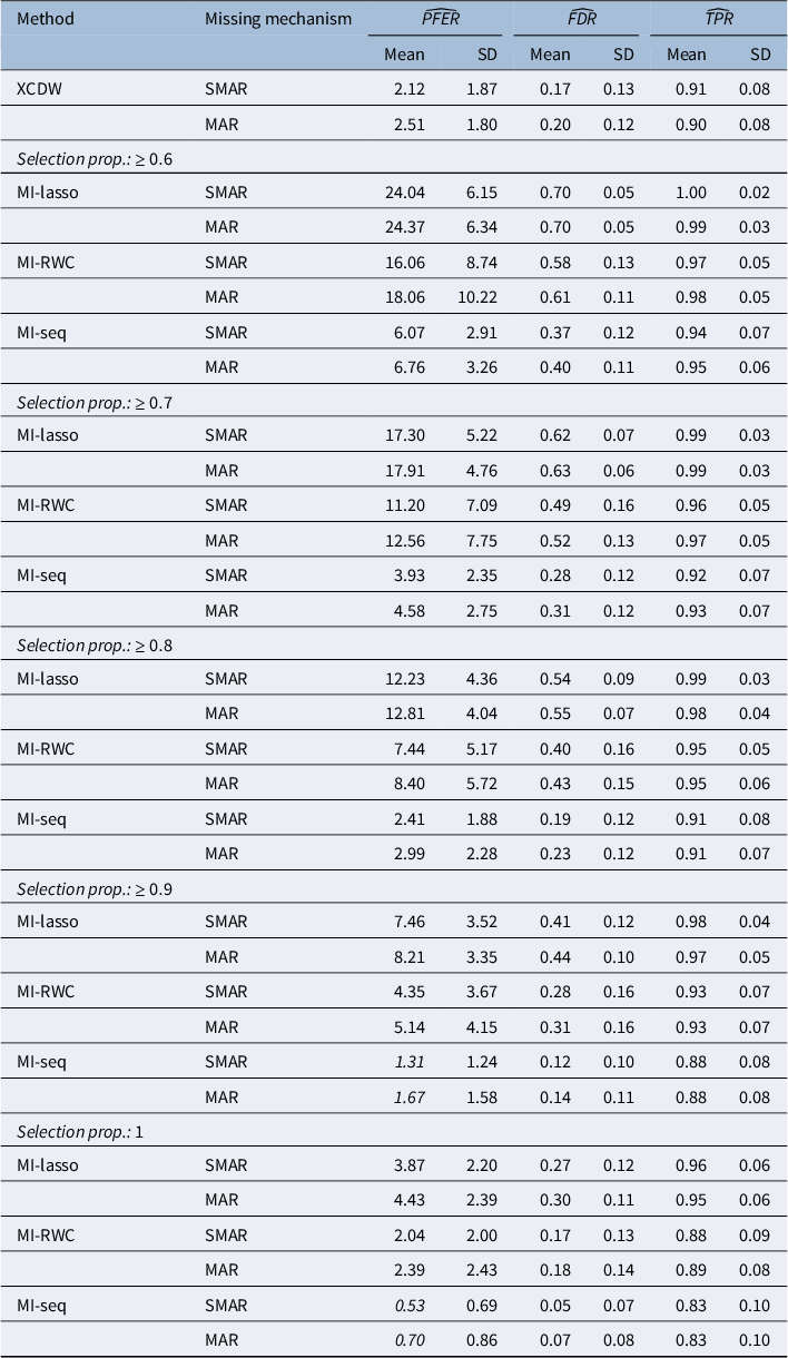
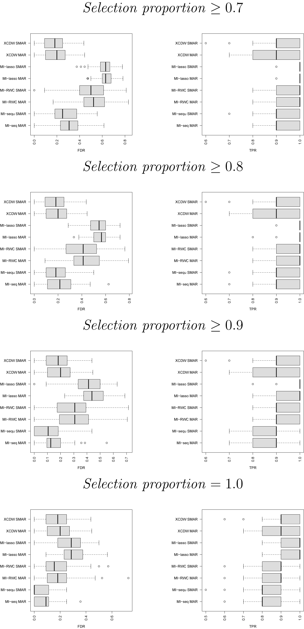


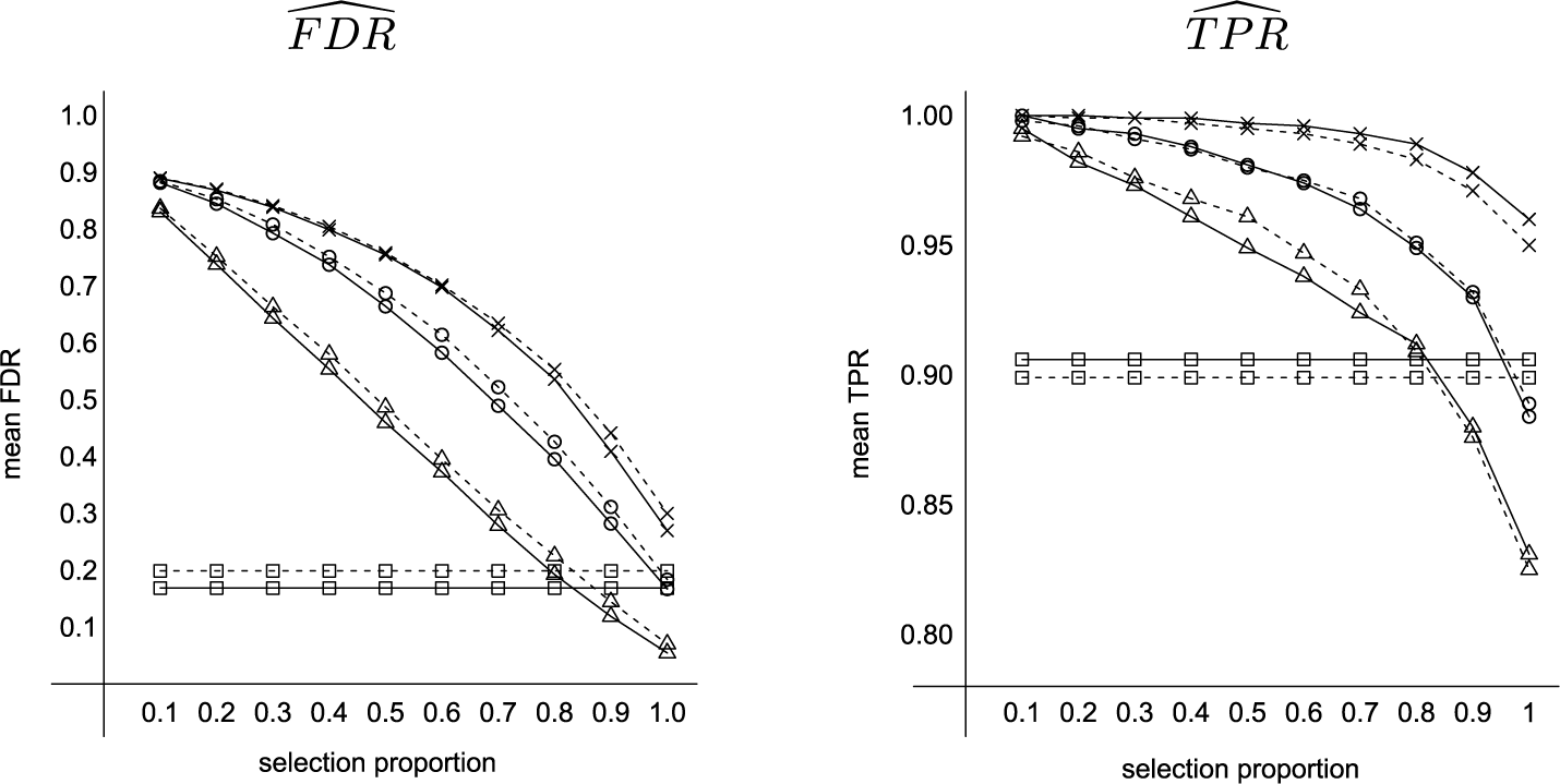


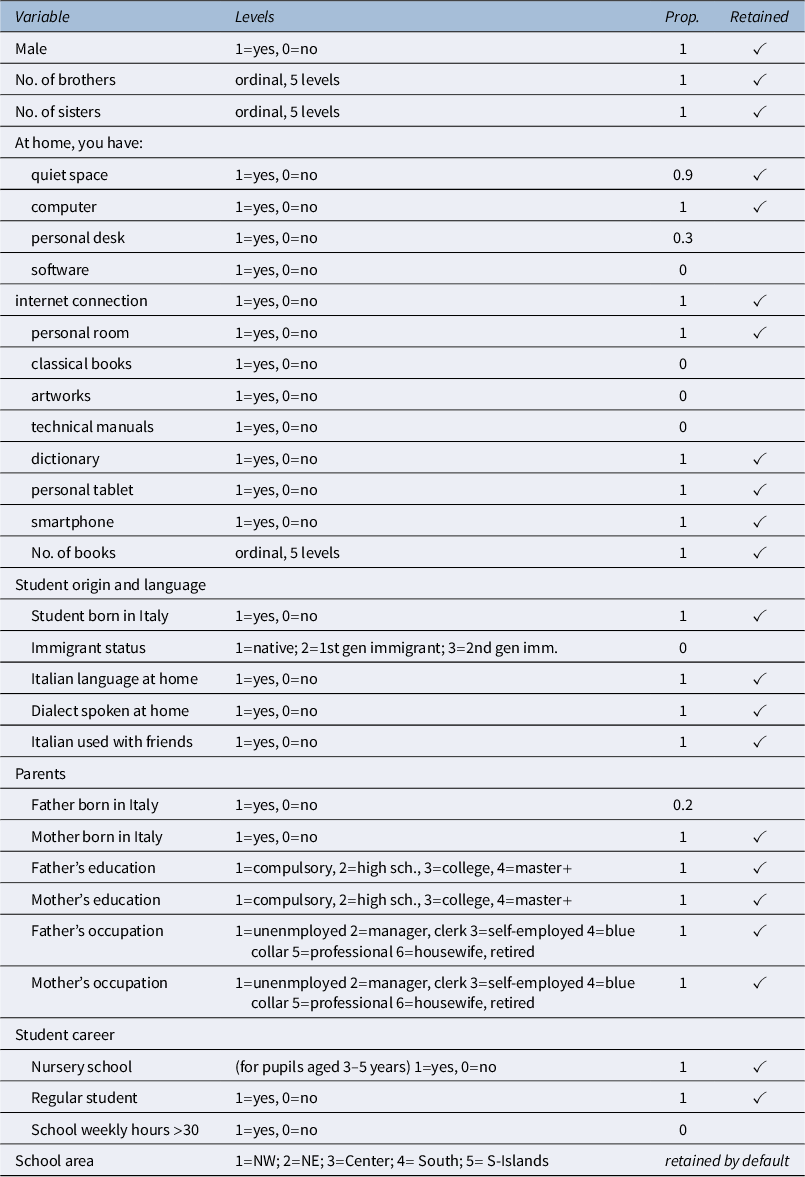


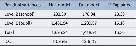
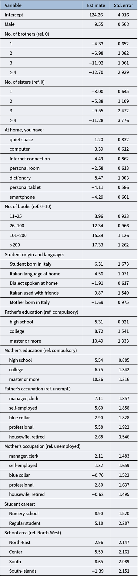
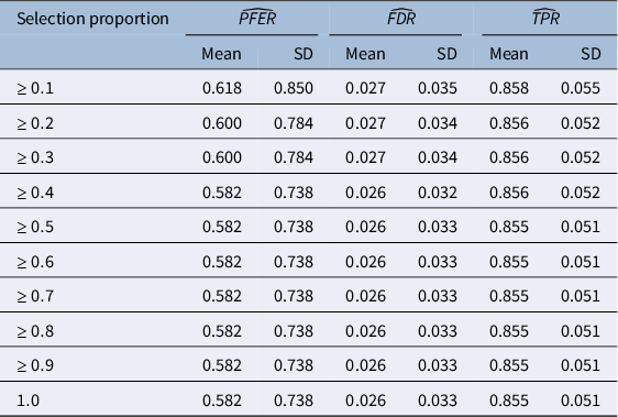


 Open access