


Introduction
Glacier melt contributes significantly to streamflow and is important for hydro-electric power generation and irrigation in many places around the world (IPCC, 2014). Glacier melt is also contributing to the global sea-level response to climate change (Radić and Hock, Reference Radić and Hock2014). To address the effects of ongoing and future glacier changes on water resources, glacier-related hazards and sea-level rise, managers and policy-makers depend on the output from melt models driven by climate data. Being able to quantify the uncertainties in estimated glacier melt provides decision-makers a basis for assessing risks associated with different management options.
The physical processes controlling glacier surface melt are well understood and energy-balance models are accurate at a range of scales (Hock, Reference Hock2005). However, energy-balance models are computationally demanding and require extensive input data that may not be available or reliable over large regions. Temperature-index models (TIM) only require air temperature as an input, which can often be interpolated from ground-based weather stations or extracted from reanalysis products with reasonable accuracy at the basin scale (Stahl and others, Reference Stahl, Moore, Floyer, Asplin and McKendry2006; Rienecker and others, Reference Rienecker2011; Trubilowicz and others, Reference Trubilowicz, Shea, Jost and Moore2016; Gelaro and others, Reference Gelaro2017). TIM are adequate for a wide range of applications and can even exceed the performance of energy-balance models when forcing data are limited (Gabbi and others, Reference Gabbi, Carenzo, Pellicciotti, Bauder and Funk2014; Réveillet and others, Reference Réveillet2018). However, the physical processes explicitly represented in energy-balance models are reduced to simplified, site-specific empirical parametrizations in TIM, which may limit their transferability.
Debris-covered glaciers are a relatively small but significant part of the global cryosphere. Estimates vary, but recent work found 4.39% (Scherler and others, Reference Scherler, Wulf and Gorelick2018) to 16.8% (Sasaki and others, Reference Sasaki, Noguchi, Zhang, Hirabayashi and Kanae2016) of the global glacierized area outside Greenland and Antarctica to be debris-covered – up to 47.4% by region. Theory, models and recent observations suggest the extent of supraglacial debris cover is increasing as glaciers recede (Bozhinskiy and others, Reference Bozhinskiy, Krass and Popovnin1986; Mayer and others, Reference Mayer, Lambrecht, Hagg and Narozhny2011; Scherler and others, Reference Scherler, Wulf and Gorelick2018). The accuracy of models of debris-covered glacier melt is therefore an increasingly important area of research.
The surface exchanges of mass and energy that lead to ice melting under debris are different to those of snow, firn and ice, because debris temperatures can exceed 0°C. In most conditions, sublimation is expected to be negligible under debris so that surface ablation occurs entirely by melt (Bozhinskiy and others, Reference Bozhinskiy, Krass and Popovnin1986; Conway and Rasmussen, Reference Conway and Rasmussen2000). Like melt of bare ice, sub-debris melt has been well reproduced by energy-balance models applied at point and glacier scales (Nakawo and Young, Reference Nakawo and Young1982; Haidong and others, Reference Haidong, Yongjing and Shiyin2006; Reid and Brock, Reference Reid and Brock2010; Reid and others, Reference Reid, Carenzo, Pellicciotti and Brock2012; Lejeune and others, Reference Lejeune, Bertrand, Wagnon and Morin2013; Brown and others, Reference Brown2014; Collier and others, Reference Collier, Nicholson, Brock, Maussion, Essery and Bush2014). However, the observational data to develop, calibrate and drive energy-balance models are as rare in debris-covered environments as elsewhere. As an alternative, a number of empirical models based on the temperature index approach have been developed for sub-debris melt (Booker and Dunbar, Reference Booker and Dunbar2008; Carenzo and others, Reference Carenzo, Pellicciotti, Mabillard, Reid and Brock2016; Möller and others, Reference Möller, Möller, Kukla and Schneider2016).
Observations show that melt rate and its sensitivity to meteorological forcing decreases as debris thickness (h) increases from an effective thickness (h c) of around 0.02–0.05 m (Østrem, Reference Østrem1959; Reznichenko and others, Reference Reznichenko, Davies, Shulmeister and McSaveney2010; Singh and others, Reference Singh, Banerjee, Nainwal and Shankar2019). Many debris-covered glacier TIM include a dependence on debris thickness and some include additional variables such as incident solar radiation (e.g. Zhang and others, Reference Zhang, Liu and Ding2007; Ragettli and others, Reference Ragettli, Pellicciotti, Bordoy and Immerzeel2013; Ayala and others, Reference Ayala2016; Carenzo and others, Reference Carenzo, Pellicciotti, Mabillard, Reid and Brock2016; Möller and others, Reference Möller, Möller, Kukla and Schneider2016; Hagg and others, Reference Hagg2018). Few studies have quantified the transferability of empirical sub-debris melt models, or the associated uncertainty in melt estimates.
The key parameter in TIM is the melt factor (k) that relates melt to air temperature. Melt factors have been applied to predict melt of debris-covered glaciers in at least 16 reported studies. The melt factors applied in those 16 studies, listed in Tables 1 and 2, vary over two orders of magnitude. Only three of the 16 values were calculated using measurements of melt; the remaining 13 melt factors were calculated using melt modeled with an energy-balance scheme, modeled as a function of bare ice melt, modeled using an assumed statistical distribution, or defined a priori. There is currently no statistically robust method for selecting melt factors for debris-covered glaciers where data for calibration are unavailable, and the accuracy of predictions made with transferred, assumed or modeled melt factors remains difficult to quantify.
Classical sub-debris melt factors, k (mm°C−1δt −1), that have been applied to model sub-debris melt with time intervals (δt) of an hr = hour, d = day or m = month

Subscript i is for bare ice, snow or both. h is debris thickness (m), and k R denotes a restricted melt factor calculated with air temperature as one of a set of predictor variables.
Restricted sub-debris melt factors, kR, calculated with air temperature as one of a set of predictors, that have been applied to model sub-debris melt
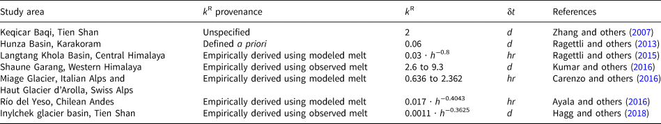
Units and notation as in Table 1.
No studies appear to have examined the effect of the provenance of air temperature data on the accuracy of transferred sub-debris melt factors, which has been shown to affect the transferability of k for bare snow and ice (Lang and Braun, Reference Lang and Braun1990; Hock and others, Reference Hock, Radić and De Woul2007; Wheler and others, Reference Wheler, MacDougall, Flowers, Petersen, Whitfield and Kohfeld2014). Consequently, it is unclear whether sub-debris melt factors calculated using air temperature data measured at an on-glacier weather station, for example, can be used to accurately predict melt using input data interpolated from a remote weather station or gridded climate data.
Gridded climate reanalysis products are increasingly used in hydrological and glaciological modeling because they provide broader spatial and temporal coverage and continuity than many traditional data sources (e.g. Koppes and others, Reference Koppes, Rupper, Asay and Winter-Billington2015; Hagg and others, Reference Hagg2018). However, if data provenance is critical to the accuracy of TIM, it would be inappropriate to use climate reanalysis data with melt factors derived from ground-based temperature observations; instead, k derived from climate reanalysis air temperature would be required.
A popular reanalysis product is The Modern-Era Retrospective analysis for Research and Applications, Version 2 (MERRA-2) from the US National Aeronautics and Space Administration (NASA). It provides surface climate fields from 1980 to present, lagging a few weeks behind real time. It has six-hourly temporal resolution and 0.5° × 0.65° spatial resolution. It has been applied successfully to model melt of debris-free glaciers over extended regions (Mernild and others, Reference Mernild, Liston and Hiemstra2014). Application of MERRA-2 to model melt of debris-covered glaciers has not yet been tested.
The objectives of this study were to (1) quantify the accuracy of classical TIM and extended TIM for debris-covered glaciers, (2) test whether air temperature data provenance affects prediction accuracy, (3) derive a generalizable relation for sub-debris melt factors that can be transferred with a known margin of error, and (4) evaluate the usefulness of MERRA-2 data for modeling sub-debris glacier melt.
Definition and calculation of melt factors
Temperature index models relate surface ablation to air temperature as follows:

where A is cumulative ablation (mm w.e.) over an observation period, k is the melt factor and PDD is the sum of positive degree-days (°C Δt). Thorough reviews of temperature index modeling of debris-free glaciers were given by Ohmura (Reference Ohmura2001) and Hock (Reference Hock2003). Time steps (δt) vary between studies (e.g. hours, days or months), which makes it difficult to directly compare values of k. In practice, δt = 1 day is most common, so the units of k are mm w.e. °C−1 d−1. For simplicity and to permit direct comparison, only data and models for δt = 1 day are included in this analysis. The following relation is used to calculate PDD:

where T is mean air temperature for each day, subscript i is one day in the observation period of n d days, T b is a threshold air temperature below which ablation ceases and δ(T) is a binary variable that sets ablation to zero below the temperature threshold. T b is often set to 0°C, but non-zero values have been found in some studies (Pellicciotti and others, Reference Pellicciotti, Buergi, Immerzeel, Konz and Shrestha2012). In this work, ablation was standardized as a mean rate, a (mm w.e. d−1):

and mean positive degree-days, D (°C), were used to enable comparison, calculated as

In this paper, the term ‘classical’ is used to distinguish melt factors calculated with only air temperature and debris thickness as the predictors (k), as in Table 1. Extended models with one or more predictors in addition to air temperature, such as incident shortwave radiation or surface slope, have been developed with a range of different formulations (e.g. Hock, Reference Hock1999; Pellicciotti and others, Reference Pellicciotti, Brock, Strasser, Burlando, Funk and Corripio2005; Carenzo and others, Reference Carenzo, Pellicciotti, Mabillard, Reid and Brock2016; Möller and others, Reference Möller, Möller, Kukla and Schneider2016). When air temperature is one of a larger set of predictor variables, as in Table 2, the coefficient associated with air temperature is called a ‘restricted’ melt factor (k R) (Kustas and others, Reference Kustas, Rango and Uijlenhoet1994). Restricted melt factors are not directly comparable to classical melt factors. Models with restricted melt factors, including predictors in addition to air temperature and debris thickness (such as solar radiation or surface characteristics), are called ‘extended TIM’.
Data collection and preparation
Overview
Data for this study were gathered from free digital archives. Observed cumulative melt, A, melt rates, a, and melt factors, k o, were compiled from existing publications. A literature search was conducted through the University of British Columbia library databases and Google Scholar using combinations of the keywords ‘glacier’, ‘ice’, ‘debris’, ‘rock’, ‘ablation’, ‘melt’, ‘melt factor’, ‘temperature index’, ‘empirical’ and ‘model’. Metadata in the publications were also collected, including geographic coordinates and site elevation, observation date and period, observational set-up, debris thickness, lithology and texture and observed air temperature. If the resolution of the geographic coordinates was low, Google Earth Pro was used to ground-truth and adjust them to a rough mid-point within the debris-covered area of each glacier (as it appears in the composite images in Google Earth Pro). Additional spatial data representing elements of the surface energy balance at the time and place of observation were collected to explore causes of variability in the observations. These were taken from MERRA-2 climate reanalysis and WorldClim V2, additional publications and geological maps. The data are included in the Supplementary Material. Procedures followed in data collection are detailed below.
The symbols, units and resolution of the data and variables used are listed with data sources in Table 3. Throughout this paper, data provenance is distinguished by a letter. The subscript ‘o’ stands for ‘observed’ and is used to identify variables, models and metrics associated with observational data copied directly from the literature. The letter ‘M’ is used to distinguish variables extracted from MERRA-2, or melt factors calculated using MERRA-2 air temperature data with observed melt rates. The letter ‘P’ stands for ‘pooled’, and is used for the observational and MERRA-2-derived melt factors combined as a single variable. The letter ‘d’ is used for melt factors calculated for Dokriani Glacier alone, using MERRA-2 air temperature data and observed melt rates.
Data and variables

Continentality, C, is computed as an annual mean value. All other numeric predictor variables are daily means.
Melt rates and melt factors
The observational data are from 27 individual glaciers located in North America, Europe, Asia, Svalbard, Iceland and New Zealand, with observation points ranging from 140 to 5350 m a.s.l. and −43 ° to 78 ° latitude. The data are individual measurements of melt and were copied directly from text and tables or by digitizing plots. In the instances where corresponding values of a and k o were published together, both were used, but separately. New melt factors, k M, were computed using Eqn (1) with observed melt rates and mean positive degree-days calculated with MERRA-2 air temperature data, D. Four complete years of data from Dokriani Glacier, Central Himalaya, which were published in Pratap and others (Reference Pratap, Dobhal, Mehta and Bhambri2015), were generously contributed as a data file by those authors. As a subset of k M, melt factors calculated for Dokriani Glacier are denoted k d.
A total of seven observations from the period before 1980 were found in the literature: one from a 1956 study of Isfallsglaciären published in Østrem (Reference Østrem1959), and six from a 1979 study of Peyto Glacier published in Nakawo and Young (Reference Nakawo and Young1981). The MERRA-2 climate reanalysis project covers the period from 1980 to present. To avoid introducing uncertainty by using more than one source of climate reanalysis data, this study was limited to the period from 1980 to present and the observations from Isfallsglaciären and Peyto Glacier were excluded.
‘Thick’ debris is thought to cover more than twice the area of ‘thin’ debris globally (Sasaki and others, Reference Sasaki, Noguchi, Zhang, Hirabayashi and Kanae2016). To isolate the ‘insulation effect’ of ‘thick’ debris, only data for debris thickness exceeding the critical thickness (h > h c) were included, where h c = 0.05 m for all glaciers except Summit Crater Glacier (Richardson and Brook, Reference Richardson and Brook2010), for which h c = 0.07 m was used. To allow direct comparison among sites, only ‘classical’ values of observed melt factors (k o) and studies focused on melting ice (rather than snow or firn) were included.
Following personal communication with the authors, the values of k o reported in Richardson and Brook (Reference Richardson and Brook2010) were corrected by applying a factor of 10−1, and the units of k o stated in Table 2 of Koppes and others (Reference Koppes, Rupper, Asay and Winter-Billington2015) were confirmed to be mm w.e. °C−1 d−1, not m °C−1 a−1 as stated in the text of page 7. Of multiple units for k o reported in Hagg and others (Reference Hagg, Mayer, Lambrecht and Helm2008), mm w.e. K−1 d−1 was assumed to be correct because cm K−1 d−1 would be unusually large.
Data processing was conducted using the R programming language (R Core Team, 2017) in R Studio. To allow comparison with observed air temperature reported as daily mean values, and of observation periods ranging from days to years, melt sums were converted to melt rates using Eqn (3). In all cases where melt rates were reported in units of water equivalent, the value for ice density used in unit conversion was stated in the corresponding publications to be 890 kg m−3. Therefore, both a and k o that were not reported in water equivalent units were standardized to mm w.e. with an assumed ice density of 890 kg m−3.
Two data subsets from Dokriani Glacier (n = 24) (Pratap and others, Reference Pratap, Dobhal, Mehta and Bhambri2015) and one from Pichillancahue–Turbio Glacier (n = 3) (Brock and others, Reference Brock, Rivera, Casassa, Bown and Acuña2007) were omitted because they exhibited a positive correlation between melt rate and debris thickness, indicating the insulation signal was confounded by other processes in those instances. The final dataset included 561 individual observations, consisting of 86 melt factors (from 12 different glaciers) and 482 melt rates (from 21 different glaciers, 235 from Dokriani Glacier). The glacier locations are shown in Figure 1. Observed melt factors (k o) ranged from 0.30 to 18.40 mm w.e. °C−1 d−1, and debris thickness ranged from 0.05 to 0.65 m. Melt factors computed with MERRA-2 positive degree-days (k M) ranged from 0.06 to 16.89 mm w.e. °C−1 d−1 and h from 0.05 to 1.20 m. The number of data points from each glacier, summary statistics for k o and data references are provided in Tables 6 and 7, Appendix A.
The location of debris-covered glaciers in this study (blue diamonds). Symbol size indicates the number of individual observations from each glacier, on a continuous scale. The black polygons are the Randolph Glacier Inventory (RGI) 6.0 first-order glaciological regions (RGI Consortium, 2017), labeled with their numeric IDs. The white areas are the RGI 6.0 glacier outlines, Greenland and Antarctica. The background map is based on data from naturalearthdata.com.

Air temperature, shortwave and longwave radiation, surface temperature
On-site air temperatures were provided in 17 of the source publications, either as a multi-day mean or as a time series. Daily mean air temperature for each melt observation period, T o, was assumed to be equal to the multi-day mean in the absence of a time series.
The NASA Earthdata subsetter tool (https://earthdata.nasa.gov) was used to extract meteorological data from MERRA-2 products for grid cells that contained the ground-truthed coordinates for each glacier. Four MERRA-2 data collections were used. The variable for 2 m air temperature (T2) was extracted from the collection inst1_2d_asm_Nx (2-dimensional, 1-Hourly, Instantaneous, Single-Level, Assimilation, Single-Level Diagnostics, V5.12.4; Global Modelling and Assimilation Office, (GMAO, 2015b)). Surface skin temperature (T s), incoming and net shortwave radiation (SWin, SWnet), and incoming, outgoing and net longwave radiation (LWa, LWe, LWnet) were taken from the collection tavg1_2d_rad_Nx (2-dimensional, 1-Hourly, Time-Averaged, Single-Level, Assimilation, Radiation Diagnostics, V5.12.4) (GMAO, 2015c). Grid cell elevation (E M) was extracted from the constants file, const_2d_asm_Nx (2d, Constants, V5.12.4) (GMAO, 2015a).
Elevation lapse rates (Γ) were used to adjust T2 to the elevation of observations (E o, in m a.s.l.) that was reported with k o and/or a, as follows:

for each observation site j. Two approaches were used to arrive at values for Γj. First, a constant value of 6.5°C km−1 was assumed and applied uniformly for all j. Second, free-atmosphere lapse rates were calculated for each grid cell from the tavg3_3d_asm_Nv collection (3-dimensional, 3-Hourly, Time-Averaged, Model-Level, Assimilation, Assimilated Meteorological Fields, V5.12.4) model-levels 72 and 71 (respectively, surface-adjacent and second from surface) (GMAO, 2015d) and applied site by site. The elevation-adjusted MERRA-2 air temperature variables were compared to T o to evaluate which best represented on-glacier conditions. T M with ΓC = 6.5°C km−1 was found to be in closest agreement with T o and was therefore used for the remainder of the study (see Appendix B ‘Comparison of MERRA-2 and on-site air temperature data’ for details). Positive degree-days were calculated from T M following Eqn (2) and converted to daily mean positive degree-days, D, using Eqn (4), to match the period of a.
Albedo
Albedo was extracted from the tavg1_2d_rad_Nx collection and averaged over each observation period. Given the spatial mismatch of observations and the MERRA-2 grid, and given the availability of albedo products from satellite imagery, higher resolution albedo from MODIS and Landsat 5 TM (αML) was also obtained, using Google Earth Engine. To avoid bias from patches of debris-free ice, ice cliffs and supraglacial ponds, αML was collected from nearby moraine rather than the glacier surface, and the moraine was identified manually. Cloud cover prevented the record of albedo during some of the observation periods. In those cases, values reported for the day nearest the date of observation were used. Albedo taken both from MERRA-2 and from MODIS and Landsat was found to vary with time, presumably due to the change of the incidence angle of solar radiation. Correcting such effects was beyond the scope of this study.
Debris geology
Geological information about the debris was provided in few of the source publications. When not stated in the source publication, debris rock type was found in a related publication or digital geological map. The debris was assumed to have the same lithology as the dominant basin bedrock in the absence of more specific information. The distribution of k in bins of debris geology at the order of, for example, limestone, granite and pumice, was found to be significantly different, but those results are not included because the classes were not well resolved and the analysis was inconclusive (in some cases the highest resolution geological data were 1:1M). Instead, debris rock type was redefined as metamorphic, igneous or sedimentary and included in the analysis as the categorical variable L.
Continentality
Continentality (C, in °C) was calculated as follows

where T max and T min are annual maximum and minimum monthly mean air temperatures (°C), respectively, extracted from WorldClim V2. WorldClim V2 is a 1 km2 resolution interpolated climate data product that is derived from ground-based and satellite observations (Fick and Hijmans, Reference Fick and Hijmans2017), which is widely cited for a variety of applications and is freely available from worldclim.org. WorldClim is a purely observational data product with structure and resolution that is appropriate for climate-scale analyses with minimal data storage and processing. The relatively high temporal and spatial resolutions of MERRA-2 reanalysis products make it appropriate for synoptic scale analyses, but require data storage and processing that were impractical for calculating climatic continentality in the current application.
Statistical analysis
Model fitting
Model fitting and analysis were performed using the R programming language (R Core Team, 2017) within R Studio. R packages used in addition to base R are listed at the end of this document and the R code is included in the Supplementary Material. The statistical models presented here are specified in R syntax rather than matrix notation, a practice that is encouraged for clarity and reproducibility (e.g. Gandrud, Reference Gandrud2015; Mair, Reference Mair2016). Readers are directed to Bates and others (Reference Bates, Mächler, Bolker and Walker2015) for mathematical expression of the R syntax.
Models were fitted separately for the two different types of melt factor, k o (observed) and k M (calculated). The melt factors calculated for Dokriani Glacier, k d, were included in the analysis of k M and also analyzed separately. This resulted in three sets of models, one for each of k o, k M and k d. Hereafter, these model sets are called KO, KM and KMd, and each individual model within a set is designated by a number (i.e. KO1, KM1, KMd1). An additional model set, KP, was generated by pooling k o and k M. The same data were not repeated in the pooled dataset. Melt factors in the KO dataset were prioritized over the KM dataset. If melt rates corresponding to the melt factors in the KO dataset were available, those melt rates were used to calculate values of k M that were included in the KM dataset but were not included in the pooled dataset.
A range of logarithmic and exponential transformations of the response and predictor variables were tested to meet the linear modeling assumption of normally distributed error terms. Models with base-10 logarithmic transformation of the response variable met that requirement and were the most accurate in cross-validation. The base-10 logarithms of the melt factors are denoted y.
An attempt was made to model ablation directly as a function of the predictor variables rather than from a predicted melt factor. However, those models were consistently less accurate than those based on a predicted melt factor and are not considered further.
Both fixed-effects and mixed-effects linear models for y were fit, the latter to account for the variability of model coefficients among glaciers and among years of observation. The motivation for using mixed-effects models in this study is that they explicitly address the hierarchical structure of the dataset when observations are grouped – e.g. by repeat sampling of the subjects in a study – and the dependency of the error terms on grouping levels (e.g. sampling sites) must be accounted for (Gałecki and Burzykowski, Reference Gałecki and Burzykowski2013; Galwey, Reference Galwey2014).
Mixed-effects models include both fixed effects and random effects. Fixed effects represent the effects of predictors that are assumed to apply uniformly throughout the population of interest. When a model that only includes fixed effects is applied to data with a grouped structure (e.g. multiple observations within multiple sites), the residuals from the model often exhibit within-group correlations; for example, some sites may have dominantly positive residuals while other sites may have dominantly negative residuals. Such within-group correlation violates the assumption of independence that underlies fixed-effects models. The inclusion of site as a random effect in this case is one way to account for such within-group correlation.
The fundamental assumption underlying a mixed-effects model is that the model coefficients can vary randomly from group to group, and are drawn from a normal distribution. When predictions are made for a new group that was not in the dataset used to fit the model, the prediction is made using the fixed-effects coefficients, which are assumed to apply through the entire population. The calculated prediction limits include the uncertainty associated with the among-site variability of the random effects. Multiple random effects and fixed effects can be included in a single mixed-effects model.
Data with a grouped structure are common to many areas of earth science (e.g. Booker and Dunbar, Reference Booker and Dunbar2008; Kasurak and others, Reference Kasurak, Kelly and Brenning2011; Azócar and others, Reference Azócar, Brenning and Bodin2017), making mixed-effects modeling especially useful. To illustrate the application of mixed-effects models, consider the case of a linear relation between a response variable y and a single predictor variable x, with multiple sites and multiple observations at each site. In this case, the model could be represented as

where y ik and x ik are the ith observations of y and x at site k, B 0 and B 1 are fixed effects that are assumed to apply to the entire population of sites, b 0k and b 1k are deviations from the fixed-effects coefficients for site k, and ɛ ik is a random error term. If the model is applied to new observations at one of the sites used to fit the model, then both the fixed effects and the random effects for that site are included. However, if the model is applied to observations at a new site, then only the fixed-effects coefficients are used. With a nested data structure, such as the present case with multiple sites, multiple years of observation at each site and multiple observations in each year, the model would be

where j is the year of observation at a given site, and the index jk indicates a deviation from the relation at site k in year j. The random effects b 0k and b 1k are included when the model is applied to new observations from a site that was used to fit the model; the random effects b 0jk and b 1jk are also included if the new observations were taken in one of the site-years used to fit the model. Otherwise, for a new site, only the fixed effects are applied, as for the simpler case of Eqn (7).
The prediction limits computed for a mixed-effects model include not only uncertainty in the fixed-effects coefficients and the random error term, as is the case for fixed-effects models, but also the uncertainty associated with the variability of coefficients among sites as represented by the variances of the mixed-effects coefficients. An important advantage of using mixed-effects models is that the values of B 0 and B 1 are not biased by individual sites with large numbers of observations, as would be the case for a fixed-effects model. Fixed-effects versions of all the models tested in this study were significantly out-performed by the mixed-effects models and are not considered further.
The mixed-effects models were fit using the lmer function from the lme4 R package using maximum likelihood estimation (Bates and others, Reference Bates, Mächler, Bolker and Walker2015). Model fitting was carried out in two stages, starting with a base model including debris thickness. In R syntax, the base mixed-effects model was defined as:

where $\hat {y}$ is the base-10 logarithm of the predicted melt factor ($\hat {k_{\rm o}}$
 , $\hat {k_{\rm M}}$
 or $\hat {k_{\rm d}}$
 ), h is debris thickness and G is the name of each glacier as a categorical variable. Equation (9) contains two fixed-effects coefficients, B 0 and B 1, which are the intercept and a slope coefficient for h, and the (1|G) term indicates a set of random-effects coefficients representing a random deviation from the fixed-effects intercept for each glacier (b 0j). Base models were also tested that allowed the slope coefficient for debris thickness to vary randomly among glaciers in addition to the intercept (b 1j):

Because multiple years of data were available for a number of glaciers, the year of observation, yr, was included as an additional random effect, nested within each glacier. The following model, for example, allows both the intercept and the slope coefficient for debris thickness to vary randomly among glaciers and years (b 0jk and b 1jk):

The candidate mixed-effects base models in Eqns (9)–(11) were evaluated with the Akaike Information Criterion (AIC). The AIC is a metric that weighs model performance against parsimony, penalizing unnecessary complexity. The base model with the lowest AIC was advanced to the second stage of model development, where additional fixed-effects predictors and interaction terms were tested. Variables tested were T s, D s, SWnet, SWin, LWnet, LWa, LWe as well as rock type (L), continentality (C), albedo (αM and αML) and RGI 6.0 glaciological region (R). To minimize issues with collinearity, pairs of predictors with a Pearson's correlation coefficient > 0.5 were not included in a model together. Otherwise, combinations of the fixed-effects variables and interaction terms, such as h · SWnet, h + SWnet + C and h + SWnet · C, and so on, were tested exhaustively. Calculated melt factors for Dokriani Glacier varied through the ablation seasons of 2010–2014. In the models for Dokriani Glacier (model set KMd), month was included as a fixed effect, and yr as a random effect.
The fitted coefficients and 95% prediction limits calculated by the lmer function are the average of the maximum likelihood estimates from a user-defined number of simulations. Here, the number of simulations per iteration was set to 10,000. Models were discarded if any individual predictor was not significant at the 0.95 confidence level or if any fitted coefficient was physically unrealistic. Valid models for each response variable were ranked by AIC. Up to five of the top-ranked models were selected for cross-validation. Only the fixed-effects coefficients were used in model validation, when fitted models were used to make predictions for glaciers not included in the model fitting.
Model validation
Leave-one-out cross-validation was used to evaluate the candidate models’ ability to reproduce observed melt rates. At each iteration, the input values for one glacier were withheld and the model fit using data from the other glaciers. The newly fitted model was then applied to predict the values for the withheld glacier. For model set KMd, 150 m elevation bins were used in place of glaciers.
Smearing estimates (s) were calculated to avoid the introduction of bias during back-transformation of the predicted values from base-10 logarithms (i.e. $\hat {k} = 10^{\lpar \hat {y} + s\rpar }$ ) (Duan, Reference Duan1983). Predicted melt rates, $\hat {a}$
 , were calculated using Eqn (1) and the back-transformed melt factors (i.e. $\hat {a} = \hat {k} \cdot D$
 ). When discussing predicted values of $\hat {y}$
 and $\hat {a}$
 , subscripts are used to indicate which model was used (e.g. $\hat {y}_{{\rm KO}3}$
 , $\hat {a}_{{\rm KM}1}$
 ).
).
Metrics used to evaluate the performance of the models in cross-validation were the root-mean-square error (RMSE), root-mean-square relative error (RMSRE), mean bias error (MBE) and relative mean bias error (RMBE), calculated as follows:


where a i and $\hat {a}_i$ are the observed and predicted values, respectively, for each observation i, and n is the total number of observations. The percentage of points within $\pm 25\percnt$
 error and the graphical linearity of the predictions also served as indicators of the models’ goodness of fit. Models that performed relatively poorly in cross-validation were discarded and a maximum of three top-performing models for each model set are presented in the Results. A range of prediction uncertainty was estimated for the strongest model in each set, where the 95% prediction limits were converted to a percentage of the predicted values and averaged over the observations.
Air temperature data provenance
To test whether melt factors calculated with air temperature data of different provenances were significantly different, k o and k M were combined as a single response variable, k P. Air temperature data provenance was included in the base model as a fixed-effects categorical predictor (i.e. observed or MERRA-2). Significance of the provenance variable was evaluated at the 0.90 confidence level. This liberal threshold was chosen to reduce the chance of incorrectly accepting the null hypothesis, that k o and k M came from the same distribution.
The importance of using air temperature data of the same provenance for both calculation and application of melt factors was also evaluated. Model set KO was tested twice, once using observed air temperature as input and again using MERRA-2 air temperature as input. If the provenance of air temperature data (i.e. MERRA-2 vs observed on-site) had a significant affect on predictive accuracy, then $\hat {a}$ calculated with $\hat {k_{\rm o}}$
 and observed positive degree-days should be more accurate than $\hat {a}$
 calculated with $\hat {k_{\rm o}}$
 and MERRA-2 positive degree-days.
A complication in the second analysis is that values of k o were calculated with observed positive degree-days, which were not reported in the source publications and were thus unavailable for this test. Therefore, the mean observed temperature, T o, was used rather than positive degree-days, whereas the MERRA-2-based temperature statistic, D, was computed as positive degree-days. It is possible that using different statistics for the calculation and application of melt factors (i.e. positive degree-days vs daily means) could affect prediction accuracy. To evaluate that possibility, cross-validation of all the models was performed with D first, and then using daily mean MERRA-2 air temperature, T M. Differences in the RMSE and MBE of the same model but different air temperature input statistic were consistently < 0.001 mm w.e. d−1. Therefore, applying T o and D in the KO models was deemed to be a valid indicative test of the effect of input data provenance on prediction accuracy. Values of $\hat {a}_{{\rm KO}}$ predicted using T o and D are distinguished with T or D appended to the model name (i.e. $\hat {a}_{{\rm KO}2-{\rm T}}$
 , $\hat {a}_{{\rm KO}2-{\rm D}}$
 ).
).
Once the significance of air temperature data provenance had been assessed, the full model fitting and validation procedures were carried out with the pooled melt factors, k P, as the response variable. That resulted in the additional set of models designated KP.
Results
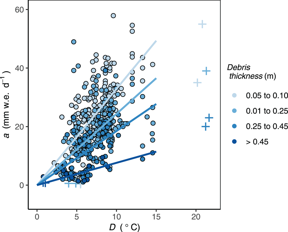
Models were fitted for the KO, KM, KP and KMd datasets, with a total of 557 individual observations from 27 glaciers around the world. From the original 568 observations, 11 values of a from Hinarche Glacier, Dokriani Glacier and Koxkar Glacier were unusually high or low given D and were removed as outliers prior to model fitting (Fig. 2, crosses). None of the predictor variables explained those values and the results presented below are for the reduced dataset (n = 557).
Observed melt rate (a) and mean daily positive degree-days based on MERRA-2 air temperatures (D), with least-squares best-fit lines through the origin for bins of debris thickness. Crosses are extreme values that were removed for model fitting.
The model coefficients presented below are in log base-10 transformed units. For example, the coefficients for the intercept, B 0, are in units of log 10 (mm w.e. °C −1 d−1), while the coefficients for debris thickness, B 1, are in units of log 10 (mm w.e. °C−1 d−1)m−1.
Dependence of ablation on degree-days and debris thickness: overview
Figure 2 illustrates the dependence of measured melt rate on positive degree-days and debris thickness. As expected, both the magnitude of melt and its sensitivity to air temperature decline as debris thickness increases. Also notable is the high degree of variability around the best-fit linear regression lines for each thickness bin.
Model set KO: melt factors for multiple glaciers extracted directly from the literature
In these models, the slope coefficient, B 1, is the direct dependence of melt factors on debris thickness, while the intercept, B 0, is the variation of melt factors that is independent of debris thickness. As seen in Table 4, the strongest models for predicted values of the log base-10 of k o are the base model with random effects in the intercept of h by glacier (G), KO1, and the extended model including SWnet, KO2. Despite the inclusion of SWnet in KO2, which results in different estimates of the intercept, the models have consistent estimates of the coefficient for debris thickness, B 1.
Fitted coefficients with standard errors and AIC for models of $\hat {y}_{{\rm KO}}$ , $\hat {y}_{{\rm KM}}$
 , $\hat {y}_{{\rm KP}}$
 and $\hat {y}_{{\rm KM_d}}$
 .
.

G is a class variable representing individual glaciers. B 0 to B 2 are fitted fixed-effects coefficients. Also shown is the number of data points in each model set, n. Random-effects coefficients are not shown. The model in each set that was most accurate in cross-validation is highlighted with bold font
Although the AIC of model KO1 is 2.4 points lower than that for KO2, model KO2 was more accurate in cross-validation (Table 5). The models have similar biases, but the RMSE and RMSRE of $\hat {a}_{{\rm KO}2}$ are almost half the magnitude of those of $\hat {a}_{{\rm KO}1}$
 . The percentage of points within ± 25% error is not a strong metric of the performance of the KO models, because the influence of individual points in the small validation dataset was exaggerated. Nonetheless, those values are also favorable to model KO2, irrespective of which air temperature input was used. Differences due to the air temperature input variable are discussed with the results for air temperature data provenance, below.
Cross-validation metrics for predicted melt rates, $\hat {a}$

The most accurate model in each set is highlighted with bold font.
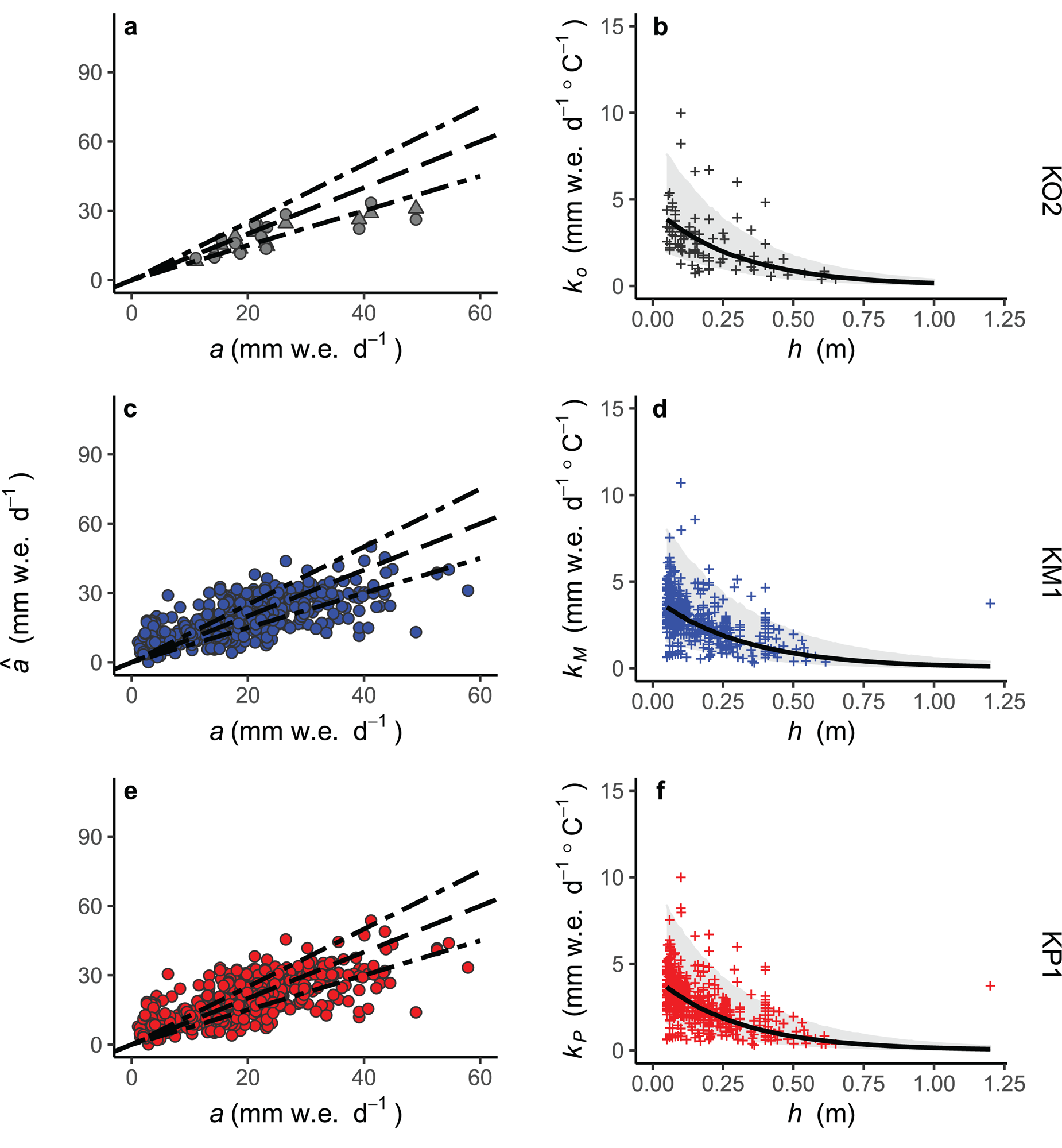
There is a negative bias in $\hat {a}_{{\rm KO}2}$ that increases as a increases (Fig. 3a), as a result of the uneven distribution of observations in the lower range of h (Fig. 3b). The 95% prediction limits for $\hat {k}_{{\rm KO}2}$
 (calculated with SWnet set to its mean value, 225 W m2) range from −49 to 203% of the predicted values on average.
Left column: observed melt rates, a, and modeled melt rates, $\hat {a}$ , using the best models for k o, k M and k P (rows 1–3, respectively). MERRA-2 positive degree-days were used as input to models KM1 and KP1. In plot a, $\hat {a}_{{\rm KO2-T}}$
 and $\hat {a}_{{\rm KO2-D}}$
 are represented with triangles and dots, respectively. The solid lines represent perfect agreement and the dashed lines are ± 25% error. Right column: observed melt factors, k (crosses), modeled melt factors, $\hat {k}$
 (curves) and 95% prediction limits (shaded areas), against debris thickness, h.
Model set KM: melt factors for multiple glaciers calculated with observed melt rates and MERRA-2 air temperature
The best KM models are the base model with random effects in the slope and intercept by glacier and by year (KM1), the model extended with αM (KM2), and the model extended with LWnet (KM3). The estimated coefficients for h are consistent between models KM1, KM2 and KM3 and consistent with those of the KO models, within the standard errors of the estimates.
Model KM2 has the lowest AIC but performed poorly by all criteria in cross-validation, with RMSE and MBE an order of magnitude larger than those of models KM1 and KM3, as seen in Table 5. Models KM3 and KM1 performed similarly well to each other, with differences in the errors on the order of 0.1 mm w.e. d−1 and one percentage point; on the basis of fractionally more favorable metrics and parsimony, the base model is deemed to be more robust.
Like $\hat {a}_{{\rm KO}2}$ , around half the values of $\hat {a}_{{\rm KM}1}$
 fell within ± 25% error, but the MBE of KM1 is an order of magnitude smaller than that of KO2. The RMSE is also smaller for $\hat {a}_{{\rm KM}1}$
 than $\hat {a}_{{\rm KO}2}$
 , but the RMSRE is around three times as large. The RMSRE was strongly influenced by the lack of observations of low melt rates in the k o dataset with which to test KO2, as seen in Figures 3a and c. It can be seen in Figure 3d that the 95% prediction limits for $\hat {k}_{{\rm KM}1}$
 are also wider than those for $\hat {k}_{{\rm KO}2}$
 , ranging from approximately −38 to 270% of the predicted value on average. Again, that resulted from the larger number of low melt factors in the k M dataset that were not present in the k o dataset.
Of two observations of melt rate found in published literature for h > 0.65 m, one was unusually large given D and was removed as an outlier before model fitting. The value of k M calculated for the sole remaining observation at h = 1.2 m is poorly reproduced by model KM1 and lies well above the prediction limits (Fig. 3d).
Model set KP: k o and k M pooled as a single response variable
Air temperature data provenance was not found to be significant in a model of k o and k M pooled as a single response variable, k P (p = 0.23). The cross-validation metrics in Table 5 vary between models KO given different air temperature input variables, T o and D. The RMSE and RMSRE are smaller using T o in both KO1 and KO2, but the MBE is around three times as large. The difference in the percentage of points within ± 25% error varies inconsistently between inputs. The differences between $\hat {a}_{{\rm KO2-T}}$ and $\hat {a}_{{\rm KO2-D}}$
 in Figure 3a are not striking.
In the absence of evidence that inconsistent air temperature data provenance reduced prediction accuracy, the model fitting and validation procedures were carried out with k P as the response variable. The strongest models set in KP are the base model with random effects in the slope and intercept of debris thickness by glacier and by year (KP1), and the model extended with LWnet (KP2) (Table 4). As with model set KM, the AIC for KP2 is lower than that for the base model but the base model was more accurate in cross-validation. The RMSE of KP1 is fractionally smaller than that of KP2, and KP1 has 3% more points within ± 25% error than KP2 (Table 5). The RMSRE and MBE for the two models are equal. On the basis of those metrics and parsimony, KP1 is deemed to be more robust.
Only around 50% of $\hat {a}_{{\rm KP}1}$ fall within ± 25% error, comparable to models KO2 and KM1. The RMSRE of KP1 falls between KO2 and KM1, the RMSE is lowest for KP1 and equal with KM1, while the MBE is lowest for KP1 of all the models. The uncertainty in $\hat {k_{\rm P}}$
 , ranging from −40 to 254% of the predicted value, is intermediate between KO2 and KM1.
Model set KMd: melt factors calculated for Dokriani Glacier with observed melt rates and MERRA-2 air temperature
Melt factors for the 2010–2013 ablation seasons at Dokriani Glacier, k d, were calculated using D and monthly melt measured at a network of 30 ablation stakes. In Figure 4 it can be seen that k d increased over the ablation season in all years except 2013. Figure 4 also shows that inter-site variability of k d within each month did not vary markedly from year to year. However, for May, the inter-site variability was low in 2010 and increased each year to the point that there was greater inter-site variability in May 2013 than in any other year-month. The difference between k d for June and September was found to be statistically significant in all years except 2013, while the difference between k d in July and August was not found to be significant in any year.
The variation of k d among ablation stakes for each month and year of the 2010–2013 ablation seasons.

The best models for k d are the base model with random effects in the slope and intercept by year, KMd1, and the model extended with a categorical variable for month, KMd2 (Table 4). The estimated coefficients for the slope of debris thickness, B 1, are consistent between KMd1 and KMd2, but notably smaller than those estimated for KO, KM and KP. The estimated coefficients for month, B 2, reflect the pattern of increase through the ablation season described above.
In cross-validation, the RMSE of the base model and KMd2 were equal, and KMd1 had 1% more predicted values within ± 25% than KMd2 (Table 5). However, the MBE of KMd2 is an order of magnitude smaller than that of KMd1, and the RMSRE is also fractionally smaller. Model KMd2 is deemed to be more robust primarily on the basis of the MBE.
Both KMd2 and KMd1 have smaller RMSE than the strongest multi-glacier models, but RMSRE more than three times as large. That is because the distribution of k d is skewed by the low May and June values while the multi-glacier datasets are more normally distributed. The MBE of KMd2 and KP1 are equal in magnitude, but the RMBE of KMd2 is twice as large as that of KP1. The prediction limits for $\hat {k_{\rm d}}$ , calculated as the mean for each month, are also wider than any of the multi-glacier models at −32 to 312% of the predicted value.
In Figure 5a, it can be seen that May melt rates were least well reproduced. It is also of note that, while k d were highest in September, a were relatively low. Figure 5b shows that the overall increase of k d between May and September, muted in July and August, is reflected in $\hat {k}_{{\rm KM_d}2}$ .
.
Left column: observed melt rates, a, and predicted melt rates, $\hat {a}$ , for Dokriani Glacier and each month of the ablation season, using model KMd2 and MERRA-2 positive degree-days. The solid lines represent perfect agreement and the dashed lines are ± 25% error. Right column: observed k d (crosses), predicted values, $\hat {k_{\rm d}}$
 (curves) and 95% prediction limits for each month (shaded areas), against debris thickness, h.

Discussion
The data compiled and analyzed here are from debris-covered glaciers around the world, covering a wide range of geographic and climatic settings. The analysis confirms the generality of the dependence of melt rates on positive degree-days and debris thickness that has been well documented at individual sites.
Accuracy of modeled melt factors applied to new glaciers without calibration
The best-performing models generated predictions that were within ± 25% error only around 50% of the time, while the RMSE and RMSRE of the highest performing model, 8.7 mm w.e. d−1 and 0.98 respectively, are substantial (model KP1, Table 5). This reflects the known strengths and weaknesses of empirical melt models, tending to be accurate on average but imprecise for specific times and places. The prediction limits of mixed-effects models are typically wider than those of equivalent fixed-effects models, because they explicitly consider the sample used to fit the model within the context of a broader population of glaciers to which the model might be applied (Shadish and others, Reference Shadish, Cook and Campbell2002). It is notable, therefore, that the accuracy of model KP1 is comparable to the reported accuracy of TIM transferred between neighboring debris-free glaciers (e.g. Wheler, Reference Wheler2009).
Extending classical TIM with additional predictors did not improve prediction accuracy, but increasing the size of the calibration dataset did. In cross-validation, model KO2, extended with SWnet, out-performed the base model (KO1), but the base models KM1 and KP1 out-performed the extended models KM2, KM3 and KP2. Then, KP1 predicted k o more accurately than either KO1 or KO2. This shows that increasing the size of the dataset let the underlying, common relation between k and h to be more accurately estimated, and that was more important than additional information about the surface energy exchanges.
The inability of other candidate predictors to contribute to the performance of the models suggests that positive degree-days and debris thickness are strong predictors of sub-debris melt, which is in agreement with previous findings (e.g. Möller and others, Reference Möller, Möller, Kukla and Schneider2016). It has been found that air temperature is reproduced more accurately than other variables in some climate reanalyses (e.g. Trubilowicz and others, Reference Trubilowicz, Shea, Jost and Moore2016); here, MERRA-2 air temperature was found to be in good agreement with observations (root mean squared deviation = 2.56°C, mean bias < 0.1°C, n = 32, Appendix B). The relative performance of the predictors may also have been influenced by relative accuracy of the MERRA-2 variables.
The increased volume of data used to fit models may have improved the accuracy of the distribution of melt factors as a function of debris thickness, or, with more repeat observations within the hierarchical sampling structure of the data, improved accuracy of the random-effects coefficients. The models in sets KM and KP were improved with random effects in the intercept and slope of h by glacier (G) and by year (yr), having repeat observations at multiple glaciers over multiple years. In contrast, the models in set KO were only improved by random effects in the intercept of h by G, because, despite the same sampling structure, there were not enough repeat observations for each value of G and yr to accurately estimate coefficients for the slope of h by G, or either the intercept or slope of h by yr. With more data, the fixed- and random-effects coefficients for both k M and k o were more accurately approximated.
Empirical melt models are often fit to data from a single glacier and applied to neighboring glaciers. The coefficients for debris thickness estimated in the models of Dokriani Glacier were significantly different to those estimated in the multi-glacier models sets, KO, KM and KP, while the coefficients for debris thickness estimated in the multi-glacier model sets were consistent with each other. This finding suggests that empirical models fitted using data from a single glacier are location specific, and that models fitted using data from multiple glaciers more accurately reflect the direct relation between melt, air temperature and debris thickness. Models fitted using data from multiple glaciers may, therefore, be more accurate when they are transferred between glaciers than models fitted using data from a single glacier. Indeed, the accuracy of predictions made with model KP1 for glaciers that KP1 had not been calibrated for was only fractionally lower than that of predictions made for bins of elevation on Dokriani Glacier with model KMd2, which was calibrated for Dokriani Glacier.
The fractionally higher accuracy of predictions made with model KMd2, with RMSE = 7.0 mm w.e. d−1 and MBE = 0.2 mm w.e. d−1, is likely to relate to the properties of the debris at Dokriani Glacier (e.g. rock type, porosity), which were uniform by comparison with those in the multi-glacier datasets. However, the elevations of observation sites at Dokriani Glacier were also known precisely while only a single, average or nominal value was known for most of the source data. Therefore, the accuracy of KMd2 might simply have been due to more accurate elevation adjustment of D.
Mixed-effects models are based on the assumption that the observation sites and years are sampled randomly from broader populations. In the current case, the sampled population includes only eight of 18 RGI glaciological regions and elevations < 5350 m a.s.l.; therefore, the applicability of the models and prediction limits outside that population of sites is not known.
The models could not be validated for debris thicker than 0.65 m. Model KP1 predicts k = 0.5 mm w.e. °C−1 d−1 for h = 0.65 m, decaying to 0.1 mm w.e. °C−1 d−1 for h between 1.0 and 1.2 m, which is in general agreement with empirical models of sub-debris melt in the literature (e.g. Brook and Paine, Reference Brook and Paine2012; Brook and others, Reference Brook, Hagg and Winkler2013; Hagg and others, Reference Hagg, Brook, Mayer and Winkler2014, Reference Hagg2018; Juen and others, Reference Juen, Mayer, Lambrecht, Han and Liu2014; Möller and others, Reference Möller, Möller, Kukla and Schneider2016). However, the single observation for h > 0.65 m, at h = 1.2 m from Juen and others (Reference Juen, Mayer, Lambrecht, Han and Liu2014), has a value of k M = 4 mm w.e. °C−1 d−1 that is considerably higher than the models predicted, suggesting the models might not be valid for h > 0.65 m.
Importance of air temperature data provenance
The success of TIMs relies on positive degree-days having a consistent relation to the surface energy balance. A number of studies have shown that, because air temperature data collected from different locations and/or by different methods differ (e.g. recorded at an AWS on the glacier or on a lateral moraine, or recorded at a remote weather station and lapsed to the elevation of the glacier), the accuracy of predictions can suffer if air temperature data of different provenances are used for the calculation and application of melt factors (e.g. Lang and Braun, Reference Lang and Braun1990; Shea and others, Reference Shea, Moore and Stahl2009; Shea and Moore, Reference Shea and Moore2010; Wheler and others, Reference Wheler, MacDougall, Flowers, Petersen, Whitfield and Kohfeld2014).
No clear evidence was found here that air temperature data provenance affected the magnitude of melt factors, given the considerable scatter inherent in the data. The slightly different distributions of k o and k M were not statistically significant, and differentiating between them did not improve the performance of the models. Nor did changing the provenance between model fitting and application of melt factors have a significant effect on prediction accuracy: the RMSE of the KO models was < 1 mm w.e. d−1 lower with observed air temperature input data than with MERRA-2 positive degree-days, but the MBE was more than 3 mm w.e. d−1 larger. Model KP1 was derived from melt factors calculated using data with two different provenances, yet, with input data of a single provenance (D), it was the most accurate of the multi-glacier models in cross-validation. This indicates that enlarging the imprecise dataset by combining observations from different sources was more valuable than maintaining consistent air temperature data provenance.
It is plausible that melt factors calculated with climate reanalysis air temperature data are more highly transferable than melt factors calculated with point-scale data. Micro-climates can affect air temperature recorded at point scale, while MERRA-2 air temperature variables reflect the full, integrated system of mass and energy fluxes through the modeling and assimilation process. Melt factors calculated with air temperature data that reflects the average, regional scale energy balance may more accurately predict melt under debris at new sites than melt factors calculated with point-scale air temperature data.
Variability of melt factors within the ablation season
The melt factors calculated for Dokriani Glacier, k d, were found to vary systematically through the 2010–2012 ablation seasons. Including month as a categorical variable in model KMd2 reduced the RMSRE of predictions by 0.32 and the MBE by an order of magnitude, from −1.1 to 0.2 mm w.e. d−1.
In 2010–2012, the values of k d increased significantly from June to a maximum in September, which is reflected in Figure 5b and the KMd2 coefficients for month in Table 4. Short-term observations have found that heat storage in supraglacial debris is close to zero on the order of days (Brock and others, Reference Brock, Rivera, Casassa, Bown and Acuña2007) but may be higher at seasonal scale (Nicholson and Benn, Reference Nicholson and Benn2013). The increase of values of k d between June and September at Dokriani Glacier suggests that heat accumulated in the debris layer after melting had begun, so that melt rates were increasingly sensitive to surface energy inputs. There was no significant difference between July and August values in any year. July is the first month of the monsoon in the Central Himalaya, characterized by thick cloud cover and intense rainfall. The rate of heat accumulation may have declined in response to reduced net radiation, or the increasing importance of heat advection by rainwater percolating through the debris.
The sensitivity of melt factors to debris thickness in model KMd2 was close to one-third that of the multi-glacier models, at −0.52 log10(mm w.e. °C−1 d−1)m−1. That also suggests that advection by rainwater percolation was an important mechanism of heat transfer in the debris layer. Continuous percolation of rain water at air temperature might reduce the thermal gradient in the near-surface, making the effect of debris thickness on melt energy supply less pronounced.
Very low values of k d in May 2010–2012 suggest that much of the surface heat input early in the ablation season was used to warm the debris layer and thus not immediately available to melt ice. May 2013 melt factors were higher than they were in previous years and more variable among sites than in any other month or year. Air temperature in the region of Dokriani Glacier was not significantly different in 2013 by comparison with previous years, but there were precipitation deficits in March, April and May 2013 (Kaur and Purohit, Reference Kaur and Purohit2013, Reference Kaur and Purohit2014). Further, precipitation in June 2013 was 123–191% greater than the climatic normal (Kaur and Purohit, Reference Kaur and Purohit2014, visualize.data.gov.in) indicating that macro-scale atmospheric circulation was unusual that year. With low spring snowfall, there may have been an unusual spatial distribution of heat in the debris, because warming could begin earlier at sites without snow, and that could explain the high inter-site variation of k d in May 2013. Studies of debris-free glaciers have shown that empirical models do not necessarily hold during seasonal transitions (e.g. Essery and others, Reference Essery, Morin, Lejeune and Ménard2013; Irvine-Fynn and others, Reference Irvine-Fynn, Hanna, Barrand, Porter, Kohler and Hodson2014; Litt and others, Reference Litt2019) and the same conclusion can be drawn from the poor prediction accuracy for May using model KMd2. This finding shows that antecedent conditions are sometimes important to seasonal melt at debris-covered glaciers.
More than half of the data in this analysis were from High Mountain Asia, under a climate similar to Dokriani Glacier (Fig. 1). However, no significant difference was found between melt factors or melt rates by region and there was no indication that the timing of observations systematically affected the values of k or a. Therefore, it is unclear whether the temporal variability of melt factors at Dokriani Glacier can be generalized.
Conclusions
This meta-analysis of previously published observations has demonstrated the generality of the dependence of sub-debris melt rates on positive degree-days and debris thickness. In cross-validation, empirical mixed-effects models describing melt factors as an exponential function of debris thickness have been found to predict melt rates with accuracy comparable to that reported for debris-free glacier TIMs transferred between neighboring glaciers. Predictions made for new glaciers with a model fitted with data from multiple glaciers were as accurate as those made for a single glacier with a model fitted with 4 years of data from the same glacier.
Overall, simple models were more accurate in cross-validation than models extended with additional predictors and interaction terms. There was no indication that air temperature data provenance significantly affected melt factors or prediction accuracy. Pooling melt factors calculated with observed melt rates and on-site air temperature and melt factors calculated with observed melt rates and MERRA-2 air temperature into a single large dataset improved prediction accuracy.
Melt factors calculated for Dokriani Glacier increased through the ablation season in 3 out of 4 years of observation. Low values for May in 2010–2012 suggested that energy was used to heat the debris after the spring snow pack melted, delaying the onset of the ablation season for a period on the order of days to weeks. Increasing values between June and September, as well as high inter-site variability in May 2013, suggest that heat storage in the debris layer was a significant part of the energy balance.
The models presented here can be used with MERRA-2 air temperature data to predict regional and glacier scale sub-debris melt rates with a known margin of error, which may be useful for estimating melt rates in the absence of more robust alternatives, or as a baseline for comparison with physically based models. However, the utility of the models for specific purposes may be limited by the relatively wide prediction limits. The 95% prediction limits around predicted melt factors is substantial at approximately −40 to 250% of the predicted values, which demonstrates that melt rates predicted with assumed melt factors without a margin of error may be misleading. An advantage of these models is that the uncertainty associated with predicted ablation is quantified, so this uncertainty can be considered when the output is used in further calculations (e.g. catchment water balances) or decision making.
To advance the science of sub-debris melt modeling, additional studies quantifying the transferability of empirical models would be valuable. It would be worthwhile for the models presented in this paper to be tested independently in a range of geographical settings. Only three observations of melt under debris > 0.65 m thick were found in the published literature and the models were unable to reproduce those observations. Additional observations would be valuable for testing the accuracy of predictions of melt under debris > 0.65 m thick. The importance of air temperature data provenance to predictions of sub-debris melt at higher temporal and spatial resolution should be tested. Seasonal and multi-year observational studies of debris heat storage would be useful to constrain the significance of heat storage to ice melt in different places. Finally, both empirical and physically-based modeling would benefit if the characteristics of supraglacial debris, including quantities such as porosity and grain size distribution as well as qualities such as rock type, were reported with future field-based studies.
R packages used
beepr (Bååth and Dobbyn, Reference Bååth and Dobbyn2018), bookdown (Xie, Reference Xie2018a), Cite (Schmitt, Reference Schmitt2016), compiler (R Core Team, 2017), digitize (Poisot, Reference T2011), dplyr (Wickham and others, Reference Wickham, François, Henry and Müller2018), ggplot2 (Wickham, Reference Wickham2010), ggpubr (Kassambara, Reference Kassambara2018), ggplotify (Yu, Reference Yu2019), grid (R Core Team, 2017), gridExtra (Auguie, Reference Auguie2017), here (Müller, Reference Müller2017), kableExtra (Hao and others, Reference Hao2018), knitr (Xie, Reference Xie2018b), lme4 (Bates and others, Reference Bates, Mächler, Bolker and Walker2015), lmerTest (Kuznetsova and others, Reference Kuznetsova, Brockhoff and Christensen2017), magrittr (Bache and Wickham, Reference Bache and Wickham2014), merTools (Knowles and others, Reference Knowles, Frederick and Whitworth2018), ncdf4 (Pierce, Reference Pierce2017), ncdf4.helpers (Bronaugh, Reference Bronaugh2014), ncdf.tools (Buttlar, Reference Buttlar2015), raster (Hijmans and others, Reference Hijmans2017), RColorBrewer (Neuwirth, Reference Neuwirth2014), rgdal (Bivand and others, Reference Bivand2018), rnaturalearth (South, Reference South2017a), rnaturalearthdata (South, Reference South2017b), tiff (Urbanek, Reference Urbanek2013).
Supplementary material
The supplementary material for this article can be found at https://doi.org/10.1017/jog.2020.57.
Acknowledgments
This work was partly funded by a UBC Doctoral Fellowship to AWB. Production of the manuscript was supported by a Research NSERC Grant to RDM. We thank V. Radić (University of British Columbia), A. Banerjee (Indian Institute of Science and Education and Research) and R. Shankar (The Institute of Mathematical Sciences, India) for valuable discussions and comments on draft manuscripts that improved the final product beyond measure. We thank the authors of Pratap and others (Reference Pratap, Dobhal, Mehta and Bhambri2015) for contributing their original data from Dokriani Glacier as a data file. We also thanks M. Bosilovich at NASA for prompt responses to questions and useful suggestions for working with MERRA-2, and thanks to the Scientific Editor, Joe Shea and an anonymous reviewer for comments leading to improvement of the final manuscript.
Appendix A - References for the observational data
References and summary statistics for the reported melt factors
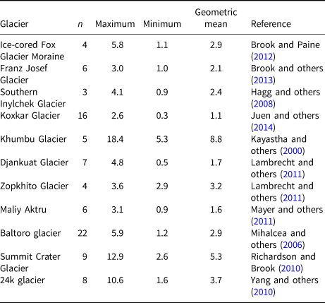
References for the reported melt rates and the number of observations at each glacier

Appendix B - Comparison of MERRA-2 and on-site air temperature data
Air temperature was reported with the melt observations in 17 of the source publications. These observations were gathered (n = 45) and standardized to daily means to inform the choice of a MERRA-2 air temperature variable to use for calculating new melt factors.
MERRA-2 data products for air temperature at 2 m and 10 m above ground were tested, extracted from the 2-dimensional assimilation instantaneous hourly collection (inst1_2d_asm_Nx) (T2 and T10). The variable T2 might be expected to agree more closely with observations made in, near or lapsed to the first few meters of the glacier surface. However, MERRA-2 2-dimensional assimilation data products represent interactions between the surface and atmosphere by a classification of surface type, where the fractional areas of land, lake, ocean and/or ice compose the surface area of a grid cell. The fractional area of each surface type is based on the aggregation of a 1 km2 resolution satellite-based global surface characterization (DISCover, Loveland and others (Reference Loveland2000)). If debris-covered glaciers were misclassified as land or if glacierization were atypical of a grid cell area, T2 could be systematically warm biased. In that case T10 could be a better approximation of point scale, ice-cooled air temperature, assuming a lapse temperature profile in the modeled air temperature fields.
Two approaches were tested to arrive at lapse rates. First, an approximate global average of 6.5 °C km−1 (ΓC) was assumed for all sites. Second, site-specific lapse rates were acquired as stated in the observation source publications (n = 3) and otherwise calculated from mid-layer air temperature of model-levels 72 and 71 from the MERRA-2 tavg3_3d_asm_Nv collection (GMAO, 2015d), as follows

where E 72 and E 71 are the model level mid-layer elevations and j is the grid cell. Lapse rates were applied following Eqn (5). Four air temperature variables resulted from this procedure, T2ΓC, T10ΓC, T2ΓM and T10ΓM, where C stands for constant and M stands for mixed. The four variables are collectively denoted TM.
The root mean squared deviation, RMSD, was used to evaluate agreement between T o and TM, calculated for every observation, i, as follows:

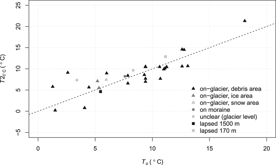
As seen in Table 8 T10 variables were smaller than they were for T2 but the difference was on the order of just 10−4 °C. The variables adjusted with a constant lapse rate were in closer agreement with observations, with RMSD around 0.2 °C smaller for both T2 and T10. Biases were found to be < 0.01 °C in all cases. The variable T2ΓC was chosen for calculating new melt factors in the meta-analysis to be consistent with the common practice of using air temperature data from the glacier near-surface and because the difference between T2ΓC and T10ΓC was slight.
The RMSD of observed air temperatures and MERRA-2 air temperatures adjusted for elevation with lapse rates

Air temperature data provenance has been found to affect the consistency of melt factors in some studies. The data for T o were recorded at automatic weather stations (AWS) that were located on the glacier being studied, on moraine near the melt observation sites, in a base camp in the same glacier basin, or in a local government-operated meteorological station, in which case the data were lapsed to the elevation of the glacier being studied. Figure 6 shows that AWS location did not have a clear affect on the deviation of T o from perfect agreement with T2ΓC.
Variables T2ΓC and T o, with symbols distinguishing T o data provenance.
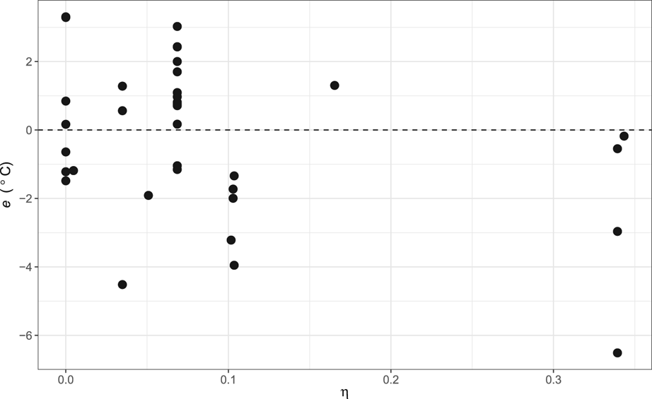
The MERRA-2 grid cell fraction of land ice (η) was nil in six instances, where the glacierized land area is small in reality (Summit Crater Glacier, Pichillancahue-Turbio Glacier, Lirung Glacier, Eliot Glacier, Miage Glacier and Ghiacciaio del Belvedere). A weak positive relationship between η and the magnitude of the deviation between T2 and T o was found, but that relationship did not remain once lapse rates had been applied. The conditions required for glacierization tend to occur at high elevation outside polar regions, and if high elevations are uncommon regionally, the difference between glacier snout elevation and mean regional elevation will be large and the glacierized area will tend to be small. A statistically significant negative linear relationship was found between η and the deviation between T2ΓC and T o (p = 0.95), as seen in Figure 7, but there is no physical reason for T2ΓC to be warm biased where η is large and cold biased where it is small. Speculatively, the pattern might reflect reduced concentration of observational air temperature data ingested to MERRA-2 with increasing ice area.
The difference between T2ΓC and T o, e, plotted against MERRA-2 grid cell fraction of land ice, η.
At sites near the coast, MERRA-2 air temperature is more strongly influenced by simulated coastal processes, which might overwhelm any signal of local interactions between the air and ice, particularly if the ice area is small. The deviation between T2 and T o was found to be slightly higher for glaciers near the coast than glaciers further from the coast but again, that was corrected with the application of elevation lapse rates, because the glaciers near the coast in these data also tend to be at relatively high elevation.


 Open access