





1 Introduction
Graph colorings have been widely studied classically. There are numerous results regarding existence of colorings for different classes of graphs. Some examples include Brooks theorem, “every graph with maximum degree n, except odd cycles or complete graphs, is n-colorable” [Reference Brooks3], and the famous four color theorem “every planar graph is
$4$
 -colorable” [Reference Robertson, Sanders, Seymour and Thomas17]. In the classical setting, most work has been focused on studying the colorings of finite connected graphs. To obtain the same results in the infinite case, one can simply apply the De-Bruijn–Erdős theorem [Reference De-Bruijn and Erdos5]. Nonetheless, colorings of infinite countable graphs might still be of interest in the sense that such colorings could be ‘computationally hard’ to find. For example, Bean showed that there exists a recursive planar graph that is
$3$
-colorable” [Reference Robertson, Sanders, Seymour and Thomas17]. In the classical setting, most work has been focused on studying the colorings of finite connected graphs. To obtain the same results in the infinite case, one can simply apply the De-Bruijn–Erdős theorem [Reference De-Bruijn and Erdos5]. Nonetheless, colorings of infinite countable graphs might still be of interest in the sense that such colorings could be ‘computationally hard’ to find. For example, Bean showed that there exists a recursive planar graph that is
$3$
 -colorable but has no recursive n-coloring for each
$n\geq 3$
-colorable but has no recursive n-coloring for each
$n\geq 3$
 [Reference Bean1]. Intuitively, this means that even if an (infinite) graph is n-colorable, such a coloring cannot be found algorithmically. In contrast, provided more colors are allowed, recursive colorings can be found [Reference Bean1, Reference Kierstead16]. A natural question that arises is whether algorithmic colorings exist for certain classes of graphs, and if such colorings do not exist, how ‘computationally difficult’ it is to find them.
To investigate the computational content of graph colorings, one possible approach is to use reverse mathematics. Reverse mathematics is a systematic approach to classifying mathematical theorems by matching them up with different levels of set existence axioms (see [Reference Dzhafarov and Mummert9, Reference Simpson20] for reference texts). The idea is to search for the weakest set existence axiom necessary for the theorem of interest to hold. This then implies that the theorem cannot be proved by any weaker set existence axiom. Most mathematical theorems fall in one of five subsystems, listed in order of strength as follows:
${\mathtt {RCA}_{0}},{{\mathtt {WKL}}}_{0},{\mathtt {ACA}_{0}},{\mathtt {ATR}_{0}}$
 , and
${\Pi _{1}^{1}-\mathtt {CA}_{0}}$
, and
${\Pi _{1}^{1}-\mathtt {CA}_{0}}$
 . Of particular interest to the present article is the subsystem
${{\mathtt {WKL}}}_{0}$
. Of particular interest to the present article is the subsystem
${{\mathtt {WKL}}}_{0}$
 which is
${\mathtt {RCA}_{0}}$
which is
${\mathtt {RCA}_{0}}$
 together with
${{\mathtt {WKL}}}$
together with
${{\mathtt {WKL}}}$
 , the assertion that each infinite binary tree has a path. Under the framework of reverse mathematics, Hirst showed that the De-Bruijn–Erdős theorem is equivalent to
${{\mathtt {WKL}}}$
, the assertion that each infinite binary tree has a path. Under the framework of reverse mathematics, Hirst showed that the De-Bruijn–Erdős theorem is equivalent to
${{\mathtt {WKL}}}$
 over
${\mathtt {RCA}_{0}}$
over
${\mathtt {RCA}_{0}}$
 and that every n-colorable graph has a low n-coloring [Reference Hirst11], thus providing an upper bound for the algorithmic content of graph colorings. Various studies have been conducted on graph coloring theorems and most have been shown to be equivalent to
${{\mathtt {WKL}}}$
and that every n-colorable graph has a low n-coloring [Reference Hirst11], thus providing an upper bound for the algorithmic content of graph colorings. Various studies have been conducted on graph coloring theorems and most have been shown to be equivalent to
${{\mathtt {WKL}}}$
 over
${\mathtt {RCA}_{0}}$
over
${\mathtt {RCA}_{0}}$
 [Reference Gasarch and Hirst10, Reference Jura15, Reference Schmerl18, Reference Schmerl and Simpson19].
Of particular interest to this article is the equivalence of the existence of colorings of planar graphs with
${{\mathtt {WKL}}}$
 over
${\mathtt {RCA}_{0}}$
over
${\mathtt {RCA}_{0}}$
 . Whilst Bean [Reference Bean1] was not working in the reverse mathematics setting, it turns out that the techniques he developed, particularly in Theorem 2 of the cited paper, together with Theorem 2.1 in [Reference Schmerl and Simpson19] gives the following.Footnote
1
. Whilst Bean [Reference Bean1] was not working in the reverse mathematics setting, it turns out that the techniques he developed, particularly in Theorem 2 of the cited paper, together with Theorem 2.1 in [Reference Schmerl and Simpson19] gives the following.Footnote
1
Theorem 1.1. For each
$n\in \omega $
 ,
${\mathtt {RCA}_{0}}+\neg {{\mathtt {WKL}}}\,\vdash\, $
,
${\mathtt {RCA}_{0}}+\neg {{\mathtt {WKL}}}\,\vdash\, $
 “There exists a planar graph that is not n-colorable.”
Together with the observation that for each
$n\geq 5$
 ,
${\mathtt {RCA}_{0}}\,\vdash\, $
,
${\mathtt {RCA}_{0}}\,\vdash\, $
 “every finite planar graph has an n-coloring”Footnote
2
and the aforementioned result that the De-Bruijn–Erdős theorem holds in
${{\mathtt {WKL}}}_{0}$
“every finite planar graph has an n-coloring”Footnote
2
and the aforementioned result that the De-Bruijn–Erdős theorem holds in
${{\mathtt {WKL}}}_{0}$
 shows that for each
$n\geq 5$
shows that for each
$n\geq 5$
 , the statement “every planar graph is n-colorable” is equivalent over
${\mathtt {RCA}_{0}}$
, the statement “every planar graph is n-colorable” is equivalent over
${\mathtt {RCA}_{0}}$
 to
${{\mathtt {WKL}}}$
to
${{\mathtt {WKL}}}$
 .
.
Closely related to the study of reverse mathematics is the study of Weihrauch reducibility. This provides a framework to compare
$\Pi _{2}^{1}$
 statements (statements of the form
$\forall X\exists Y\,\varphi $
statements (statements of the form
$\forall X\exists Y\,\varphi $
 ; X is generally referred to as an instance and Y a solution). Roughly speaking, if
$P,Q$
; X is generally referred to as an instance and Y a solution). Roughly speaking, if
$P,Q$
 are
$\Pi _{2}^{1}$
are
$\Pi _{2}^{1}$
 statements, and P is Weihrauch below Q, written
$P{\leq _{\mathsf {W}}} Q$
statements, and P is Weihrauch below Q, written
$P{\leq _{\mathsf {W}}} Q$
 , then it means that if for any Q-instance, we are able to find a Q-solution, then we can do the same for P; Q is algorithmically more complex than P. While in most cases, an implication in the setting of reverse mathematics corresponds to a Weihrauch reduction, there exists examples where an implication holds but no Weihrauch reductions can be found [Reference Dorais, Dzhafarov, Hirst, Mileti and Shafer7, Reference Jockush12, Reference Jockush13].
Another benefit of this approach is that it allows one to study the uniformity of how a proof of one statement translates into a proof of the other. For instance, it is known that for each
$k\geq 2$
 , the principles
${\mathtt {DNR}}(k)$
, the principles
${\mathtt {DNR}}(k)$
 (see Definition 2.13) are equivalent to
${{\mathtt {WKL}}}$
(see Definition 2.13) are equivalent to
${{\mathtt {WKL}}}$
 over
${\mathtt {RCA}_{0}}$
over
${\mathtt {RCA}_{0}}$
 in the reverse mathematical setting, but not uniformly so when
$k>2$
in the reverse mathematical setting, but not uniformly so when
$k>2$
 [Reference Dorais, Hirst and Shafer8, Reference Jockush13, Reference Jockush and Soare14].
Following this pattern and motivated by the reverse mathematical results concerning planar graph colorings, we study these principles under the setting of Weihruach reductions. In Section 2 we attempt to calibrate the strengths of each of the coloring principles (to be defined in Definition 1.6) according to variants of
${\mathtt {DNR}}$
 principles (see Definition 2.13, 2.21), analysing the strength of n-colorings of planar graphs for various
$n<7$
principles (see Definition 2.13, 2.21), analysing the strength of n-colorings of planar graphs for various
$n<7$
 and also obtaining certain bounds in the general case. In Section 3, we show that for all
$n\geq 7$
and also obtaining certain bounds in the general case. In Section 3, we show that for all
$n\geq 7$
 , non-uniformity in the proofs of
${\mathtt {RCA}_{0}}+\text {"Every planar graph has an }n\text {-coloring."}\,\vdash\, {{\mathtt {WKL}}}$
, non-uniformity in the proofs of
${\mathtt {RCA}_{0}}+\text {"Every planar graph has an }n\text {-coloring."}\,\vdash\, {{\mathtt {WKL}}}$
 is necessary, and also characterise the existence of Weihrauch reductions from
${\mathtt {DNR}}(k)$
is necessary, and also characterise the existence of Weihrauch reductions from
${\mathtt {DNR}}(k)$
 to
${\mathtt {COL}}(n)$
to
${\mathtt {COL}}(n)$
 (both to be defined later) as a finite graph theoretic property.
1.1 The principles and formal definitions
Since the main objective of this article is to investigate the uniform relationships between theorems on the coloring of planar graphs, we shall start with the following definitions.
Definition 1.2 (
${\mathtt {RCA}_{0}}$
 )
)

-
• A graph $G=( V,E)$
is a countable set of vertices
$V=\{v_{0},v_{1},\dots \}$
and a symmetric irreflexive binary relation
$E\subseteq V^{2}$
. We will only consider simple undirected graphs in this article. Note that we do not require a graph to be locally finite or connected. -
• A subgraph of $G=(V,E)$
is a graph
$G'=(V',E')$
such that
$V'\subseteq V$
and
$E'\subseteq E$
. A subgraph is not necessarily induced. -
• A finite graph $\widehat {G}$
is planar if neither
$K_{3,3}$
nor
$K_{5}$
is a minor of
${\widehat {G}}$
. An infinite countable graph G is planar iff every finite subgraph of G is planar. -
• Given a graph $G=(V,E)$
, we say that h is a c-coloring of G iff
$h:V\to \{0,1,\dots ,c-1\}$
and for any two vertices
$v,w$
, if
$h(v)=h(w)$
, then
$\{v,w\}\notin E$
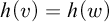
. A graph is said to be c-colorable if it has a c-coloring.










We use G to denote infinite countable planar graphs, and
$\widehat {G}$
 to refer to finite planar graphs, unless explicitly stated otherwise.
Definition 1.3 (
${\mathtt {RCA}_{0}}$
)

Given a graph
$G=(V,E)$
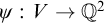
 , a diagram of G is a pair of injective functions
$\psi :V\to {\mathbb {Q}}^{2}$
, a diagram of G is a pair of injective functions
$\psi :V\to {\mathbb {Q}}^{2}$
 and
$f:E\to {\mathbb {N}}$
and
$f:E\to {\mathbb {N}}$
 such that for each
$\{u,v\}\in E$
such that for each
$\{u,v\}\in E$
 ,
$f(\{u,v\})$
,
$f(\{u,v\})$
 encodes some j-tuple of pairs of rational numbers
$ \langle \langle p_{0},q_{0}\rangle ,\langle p_{1},q_{1}\rangle ,\dots ,\langle p_{j},q_{j}\rangle \rangle $
encodes some j-tuple of pairs of rational numbers
$ \langle \langle p_{0},q_{0}\rangle ,\langle p_{1},q_{1}\rangle ,\dots ,\langle p_{j},q_{j}\rangle \rangle $
 where
$\psi (u),\psi (v)$
where
$\psi (u),\psi (v)$
 are the first and last (or last and first) entry respectively.
For a given diagram
$(\psi ,f)$
 , the restriction
$(\psi ,f)\restriction n$
, the restriction
$(\psi ,f)\restriction n$
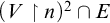
 is given by restricting the domains of
$\psi $
is given by restricting the domains of
$\psi $
 and f to
$V\restriction n$
and f to
$V\restriction n$
 and
$(V\restriction n)^{2}\cap E$
and
$(V\restriction n)^{2}\cap E$
 respectively. Intuitively,
$(\psi ,f)\restriction n$
respectively. Intuitively,
$(\psi ,f)\restriction n$
 is a diagram of the induced subgraph on the first n vertices of G.
In addition, we say that a diagram is planar (or simply a plane diagram) iff it is a diagram with the additional property that for each
$\langle p_{i},q_{i}\rangle \in f(\{u,v\})$
 and
$\langle p_{j}',q_{j}'\rangle \in f(\{u',v'\})$
and
$\langle p_{j}',q_{j}'\rangle \in f(\{u',v'\})$
 (where
$\{u,v\}\neq \{u',v'\}$
(where
$\{u,v\}\neq \{u',v'\}$
 ) the line segments from
$(p_{i},q_{i})$
) the line segments from
$(p_{i},q_{i})$
 to
$(p_{i+1},q_{i+1})$
to
$(p_{i+1},q_{i+1})$
 do not intersect with those from
$(p_{j}',q_{j}')$
do not intersect with those from
$(p_{j}',q_{j}')$
 to
$(p_{j+1}',q_{j+1}')$
to
$(p_{j+1}',q_{j+1}')$
 , except possibly at the endpoints of
$f(\{u,v\})$
, except possibly at the endpoints of
$f(\{u,v\})$
 and
$f(\{u',v'\})$
and
$f(\{u',v'\})$
 .Footnote
3
.Footnote
3
The intention behind f in the definition above is to formalise embedding of edges by finitely many straight line segments. We note that in the classical setting, having an embedding of the graph into
${\mathbb {R}}^{2}$
 is clearly equivalent to having a plane diagram in the sense of the definition above.
Definition 1.4 (Faces)
Given a plane diagram
$(\psi ,f)$
 of a finite connected planar graph
$\widehat {G}$
of a finite connected planar graph
$\widehat {G}$
 , we wish to define an encoding of the faces of the diagram. Classically, an inner face of the diagram can be defined as a bounded, non-empty, connected open region F of the plane that is enclosed by a closed walk C taken in the diagram with the property that F does not intersect the diagram. The outer face is the unbounded, connected open region F of the plane with a closed walk C forming the boundary of F with the property that F does not intersect the diagram.
Each face (inner and outer) of the plane diagram can be encoded by the closed walk forming the boundary of the face. (Recall that this is just a finite list of rational coordinates). A face-list of the plane diagram is a list of the codes of all faces of the diagram. Obviously, the face-list of a plane diagram of a finite connected planar graph can be found effectively from the plane diagram itself.
Definition 1.5 (
${\mathtt {RCA}_{0}}$
)

Given two plane diagrams
$(\psi _{0},f_{0})$
 and
$(\psi _{1},f_{1})$
and
$(\psi _{1},f_{1})$
 , we say that
$(\psi _{0},f_{0})\restriction n+1$
, we say that
$(\psi _{0},f_{0})\restriction n+1$
 and
$(\psi _{1},f_{1})\restriction n+1$
and
$(\psi _{1},f_{1})\restriction n+1$
 are equivalent if both of the following holds.
-
• $(\psi _{0},f_{0})\restriction n$
and
$(\psi _{1},f_{1})\restriction n$
are equivalent. (The restrictions
$(\psi _{0},f_{0})\restriction 0$
and
$(\psi _{1},f_{1})\restriction 0$
are always equivalent.) -
• $\psi _{0}(v_{n})$
and
$\psi _{1}(v_{n})$
are contained in the same face in
$(\psi _{0},f_{0})\restriction n+1$
and
$(\psi _{1},f_{1})\restriction n+1$
. More formally, the faces which
$\psi _{0}(v_{n})$
and
$\psi _{1}(v_{n})$
are contained in are enclosed by the same vertices and edges.






Two plane diagrams
$(\psi _{0},f_{0}),(\psi _{1},f_{1})$
 are equivalent if
$(\psi _{0},f_{0})\restriction n,(\psi _{1},f_{1})\restriction n$
are equivalent if
$(\psi _{0},f_{0})\restriction n,(\psi _{1},f_{1})\restriction n$
 are equivalent for all
$n\in {\mathbb {N}}$
are equivalent for all
$n\in {\mathbb {N}}$
 .
.
It is not difficult to see that if two plane diagrams
$(\psi _{0},f_{0})$
 and
$(\psi _{1},f_{1})$
and
$(\psi _{1},f_{1})$
 are equivalent in the sense above, then the range of
$f_{0}$
are equivalent in the sense above, then the range of
$f_{0}$
 and
$f_{1}$
and
$f_{1}$
 (as subsets of
${\mathbb {R}}^{2}$
(as subsets of
${\mathbb {R}}^{2}$
 ) are homeomorphic in the classical sense.
The common classical definition of a planar graph G is via the existence of a planar embedding of G into the plane (or the sphere). Wagner [Reference Wagner21] showed that this definition is equivalent to the one given in Definition 1.3 for finite graphs. Erdős showed that the two definitions are equivalent for infinite countable graphs (see [Reference Dirac and Schuster6]). Note that in Definition 1.3 we do not put any other topological restrictions on the range of the embedding. For instance, Dirac and Schuster [Reference Dirac and Schuster6] pointed out that there is a certain countable planar graph G such that the range of every plane embedding of G into the plane contains a limit point.
As usual, the fact that the two definitions (of planarity) are classically equivalent cannot be carried over to the effective setting. It is not hard to see that not every planar computable graph has a computable plane diagram. In fact, in Proposition 2.1, we will show that the statement “Every planar graph has a plane diagram” is equivalent over
${\mathtt {RCA}_{0}}$
 to
${{\mathtt {WKL}}}$
to
${{\mathtt {WKL}}}$
 .
.
The main objective of this article is to study the logical relationships between different statements surrounding the coloring of planar graphs. The most famous result in this area is the four color theorem. This problem is widely believed to be first raised by Francis Guthrie in 1852 while trying to color a map of the counties of England, and an incorrect proof of the four color theorem was announced by Alfred Kempe in 1879. Kempe’s proof was shown to be flawed by Percy Heawood eleven years later, who then proved the five color theorem based on Kempe’s incorrect proof. While these results are about finite planar graphs, the corresponding statements for infinite planar graphs still hold true classically, due to the well-known result of De-Bruijn and Erdős [Reference De-Bruijn and Erdos5].
This prompts us to consider the following principles, formalized in
${\mathtt {RCA}_{0}}$
 .
.
Definition 1.6 (
${\mathtt {RCA}_{0}}$
)

Let
$n\in \mathbb {N}$
 where
$n\geq 4$
where
$n\geq 4$
 .
.
-
• ${\mathtt {COL}}(n)$
is the statement that every countable planar graph is n-colorable. -
• ${\mathtt {COL}}^{*}(n)$
is the statement that every countable planar graph with a plane diagram is n-colorable. -
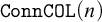
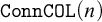
• ${\mathtt {ConnCOL}}(n)$
is the statement that every countable connected planar graph is n-colorable.


Here, a connected graph is one where every two vertices is connected by a finite path. Trivially,
${\mathtt {COL}}(n)$
 implies both
${\mathtt {COL}}^{*}(n)$
implies both
${\mathtt {COL}}^{*}(n)$
 and
${\mathtt {ConnCOL}}(n)$
and
${\mathtt {ConnCOL}}(n)$
 for each
$n\geq 4$
for each
$n\geq 4$
 . We remark here that even though every planar graph necessarily has a plane diagram,
${\mathtt {COL}}^{*}(n)$
. We remark here that even though every planar graph necessarily has a plane diagram,
${\mathtt {COL}}^{*}(n)$
 should be interpreted as a principle where upon being given as input a graph and a plane diagram of the graph, produces an n-colouring of the graph, in contrast with the principles
${\mathtt {COL}}(n),{\mathtt {ConnCOL}}(n)$
should be interpreted as a principle where upon being given as input a graph and a plane diagram of the graph, produces an n-colouring of the graph, in contrast with the principles
${\mathtt {COL}}(n),{\mathtt {ConnCOL}}(n)$
 where the input is merely a graph. As mentioned earlier, in this article, we focus on the uniform relationships between these coloring principles and other common principles like
${{\mathtt {WKL}}}$
where the input is merely a graph. As mentioned earlier, in this article, we focus on the uniform relationships between these coloring principles and other common principles like
${{\mathtt {WKL}}}$
 . More formally, we shall study them in the setting of Weihrauch reducibility, defined as follows.
Definition 1.7 [Reference Dorais, Dzhafarov, Hirst, Mileti and Shafer7] but also see [Reference Brattka and Gherardi2, Reference Weihrauch22]
Let P and Q be
$\Pi _{2}^{1}$
 statements of second-order arithmetic. We say that
-
• P is Weihrauch reducible to Q, $P{\leq _{\mathsf {W}}} Q$
, if there exist
$\Phi ,\Psi $
where
$\Phi ,\Psi $
are Turing reductions such that whenever A is an instance of P,
$B=\Phi (A)$
is an instance of
$Q,$
and if T is a solution to B, then
$S=\Psi \left (T\oplus A\right )$
is a solution of P. -
• P is strongly Weihrauch reducible to Q, $P{\leq _{\mathsf {sW}}} Q$
, if there exist
$\Phi ,\Psi $
where
$\Phi ,\Psi $
are Turing reductions such that whenever A is an instance of P,
$B=\Phi (A)$
is an instance of
$Q,$
and if T is a solution to B, then
$S=\Psi (T)$
is a solution of P.





2 The reverse mathematics of coloring principles
We first begin by addressing the question of whether the two classical definitions of planarity:
-
• G is planar if no finite subgraph of G contains $K_{3,3}$
or
$K_{5}$
as a minor, versus -
• G ‘admits a plane diagram’ if there is a planar embedding of G into the plane,


are equivalent from the point of view of reverse mathematics. Firstly, notice that if G admits a plane diagram (refer to Definition 1.3), then G is planar. For this, note that Euler’s formula and therefore the non-planarity of
$K_{5}$
 and
$K_{3,3}$
and
$K_{3,3}$
 can be verified in
${\mathtt {RCA}_{0}}$
can be verified in
${\mathtt {RCA}_{0}}$
 .Footnote
4
Therefore, the principle of interest is “Every planar G admits a plane diagram.” We prove that this is equivalent to
${{\mathtt {WKL}}}$
.Footnote
4
Therefore, the principle of interest is “Every planar G admits a plane diagram.” We prove that this is equivalent to
${{\mathtt {WKL}}}$
 .
.
Proposition 2.1. Over
${\mathtt {RCA}_{0}}$
 , the following are equivalent:
-
• ${{\mathtt {WKL}}}$
. -
• Every planar graph admits a plane diagram.

The “only if” direction is originally due to Erdős (again, see [Reference Dirac and Schuster6]), and we include a proof of it here for completeness.
Proof. First, we prove that
${{\mathtt {WKL}}}_{0}\,\vdash\, $
 “Every planar graph admits a plane diagram.” Let
$G=(V,E)$
“Every planar graph admits a plane diagram.” Let
$G=(V,E)$
 be a planar graph, and
$\{v_{i}\}_{i\in {\mathbb {N}}}$
be a planar graph, and
$\{v_{i}\}_{i\in {\mathbb {N}}}$
 be an enumeration of V. To obtain a plane diagram D, we encode for each n, all possible plane diagrams of the induced subgraph
$\widehat {G}$
be an enumeration of V. To obtain a plane diagram D, we encode for each n, all possible plane diagrams of the induced subgraph
$\widehat {G}$
 of G containing
$v_{0},v_{1},\dots ,v_{n-1}$
of G containing
$v_{0},v_{1},\dots ,v_{n-1}$
 , as a node on a tree T. Clearly, the intuition should be that a node
$\sigma $
, as a node on a tree T. Clearly, the intuition should be that a node
$\sigma $
 is extended by
$\tau $
is extended by
$\tau $
 if the diagram encoded by
$\sigma $
if the diagram encoded by
$\sigma $
 is a sub-diagram of the one encoded by
$\tau $
is a sub-diagram of the one encoded by
$\tau $
 . We provide the details below.
Recall from Definition 1.4, that given any plane diagram of a finite graph
$\widehat {G}$
 , we are able to list all its faces. Given
$\sigma \in T$
, we are able to list all its faces. Given
$\sigma \in T$
 encoding a plane diagram of the induced subgraph containing vertices
$v_{0},v_{1},\dots ,v_{n-1}$
encoding a plane diagram of the induced subgraph containing vertices
$v_{0},v_{1},\dots ,v_{n-1}$
 , since there are only finitely many vertices, then there can be only finitely many faces. For a given face, embedding
$v_{n}$
, since there are only finitely many vertices, then there can be only finitely many faces. For a given face, embedding
$v_{n}$
 anywhere within that face will result in an equivalent diagram. (Recall that each edge is represented via finitely many line segments and that our diagram is not necessarily rectilinear.) That is to say, there are only finitely many possible extensions of
$\sigma $
anywhere within that face will result in an equivalent diagram. (Recall that each edge is represented via finitely many line segments and that our diagram is not necessarily rectilinear.) That is to say, there are only finitely many possible extensions of
$\sigma $
 . Of course, this is not to say that every choice of face to embed
$v_{n}$
. Of course, this is not to say that every choice of face to embed
$v_{n}$
 in results in a valid plane diagram extending
$\sigma $
in results in a valid plane diagram extending
$\sigma $
 . In particular, if
$v_{n}$
. In particular, if
$v_{n}$
 is adjacent to some vertex not on the boundary of the face it was embedded in, this cannot be extended to a valid plane diagram extending
$\sigma $
is adjacent to some vertex not on the boundary of the face it was embedded in, this cannot be extended to a valid plane diagram extending
$\sigma $
 . Nevertheless, since there are only finitely many faces, and each face corresponds to at most one valid choice to embed
$v_{n}$
. Nevertheless, since there are only finitely many faces, and each face corresponds to at most one valid choice to embed
$v_{n}$
 , then T is G-computably branching.
Suppose to the contrary that T as described is finite. Then, there is some n such that for all
$t\in T,\,|t|<n+1$
 . For such an n, consider the induced subgraph
$\widehat {G}$
. For such an n, consider the induced subgraph
$\widehat {G}$
 containing vertices
$v_{0},v_{1},\dots ,v_{n}$
containing vertices
$v_{0},v_{1},\dots ,v_{n}$
 . Since G is planar, then
$\widehat {G}$
. Since G is planar, then
$\widehat {G}$
 must also be planar; then
$\widehat {G}$
must also be planar; then
$\widehat {G}$
 must have a plane diagram D. For each
$i\leq n$
must have a plane diagram D. For each
$i\leq n$
 , considering the positions of the vertices
$v_{0},v_{1},\dots ,v_{i}$
, considering the positions of the vertices
$v_{0},v_{1},\dots ,v_{i}$
 relative to the faces, must produce some plane diagram equivalent to one encoded by some node
$\sigma \in T$
relative to the faces, must produce some plane diagram equivalent to one encoded by some node
$\sigma \in T$
 of length
$i+1$
of length
$i+1$
 . Then there must be some node of length
$n+1$
. Then there must be some node of length
$n+1$
 in T, a contradiction to the assumption. Thus T is infinite. By bounded Konig’s lemma, there is a path h through T. Furthermore, it is clear that a planar diagram of G can then be constructed by considering
$h(n)$
in T, a contradiction to the assumption. Thus T is infinite. By bounded Konig’s lemma, there is a path h through T. Furthermore, it is clear that a planar diagram of G can then be constructed by considering
$h(n)$
 at each n. Thus we have that
${{\mathtt {WKL}}}_{0}$
at each n. Thus we have that
${{\mathtt {WKL}}}_{0}$
 proves that every planar graph G has a plane diagram.
Now we reason in
${\mathtt {RCA}_{0}}$
 and assume that every planar graph G has a plane diagram (which exists within the given model). Let T be an arbitrary infinite binary tree. Construct a countable planar graph,
$G=\langle V,E\rangle $
and assume that every planar graph G has a plane diagram (which exists within the given model). Let T be an arbitrary infinite binary tree. Construct a countable planar graph,
$G=\langle V,E\rangle $
 as follows. G will consist of countably many components, each corresponding to some binary string
$\tau $
as follows. G will consist of countably many components, each corresponding to some binary string
$\tau $
 . We thus refer to each component as the
$\tau $
. We thus refer to each component as the
$\tau $
 -th component. The
$\tau $
-th component. The
$\tau $
 -th component will originally consist of six vertices,
$v_{\tau ,i}$
-th component will originally consist of six vertices,
$v_{\tau ,i}$
 for each
$i<6$
for each
$i<6$
 . The vertices
$v_{\tau ,j}$
. The vertices
$v_{\tau ,j}$
 for each
$j<5$
for each
$j<5$
 are connected as shown in Figure 1 (note that the three drawings are all isomorphic as graphs), and
$v_{\tau ,5}$
are connected as shown in Figure 1 (note that the three drawings are all isomorphic as graphs), and
$v_{\tau ,5}$
 is connected to
$v_{\tau ,3}$
is connected to
$v_{\tau ,3}$
 . The idea is that in the
$\tau $
. The idea is that in the
$\tau $
 -th component, the position of
$v_{\tau ,5}$
-th component, the position of
$v_{\tau ,5}$
 in the diagram encodes which subtree extending
$\tau $
in the diagram encodes which subtree extending
$\tau $
 is infinite. Since there are only three distinct drawings (up to equivalence) of the first five vertices in a component, the choice of embedding of
$v_{\tau ,5}$
is infinite. Since there are only three distinct drawings (up to equivalence) of the first five vertices in a component, the choice of embedding of
$v_{\tau ,5}$
 will indicate the subtree extending
$\tau $
will indicate the subtree extending
$\tau $
 which is infinite.
-
(1) If $v_{\tau ,5}$
is contained in
$F_{i}$
for some
$i<2$
, then the subtree above
$\tau ^{\frown }i$
is infinite. -
(2) If $v_{\tau ,5}$
is contained in
$F_{2}$
, then both subtrees above
$\tau ^{\frown }0$
and
$\tau ^{\frown }1$
are infinite.


We provide the details below.
Reversal of Proposition 2.1.

Figure 1. Long description
A multi-panel figure containing three panels labeled Possible drawing 1, Possible drawing 2, and Possible drawing 3. Each panel depicts a rhombus divided into two triangles by a horizontal center line. Each rhombus has five vertices represented by black dots: one at the top, one at the bottom, one on the left, one on the right, and one in the center of the horizontal line.
In Possible drawing 1:
* The top vertex is v sub tau, 2.
* The bottom vertex is v sub tau, 0.
* The left vertex is v sub tau, 3.
* The right vertex is v sub tau, 4.
* The center vertex is v sub tau, 1.
* The upper triangle is labeled F sub 1, the lower triangle is F sub 2, and the exterior space to the top-left is F sub 0.
In Possible drawing 2:
* The top vertex is v sub tau, 1.
* The bottom vertex is v sub tau, 0.
* The left vertex is v sub tau, 3.
* The right vertex is v sub tau, 4.
* The center vertex is v sub tau, 2.
* The upper triangle is labeled F sub 1, the lower triangle is F sub 0, and the exterior space to the top-left is F sub 2.
In Possible drawing 3:
* The top vertex is v sub tau, 2.
* The bottom vertex is v sub tau, 1.
* The left vertex is v sub tau, 3.
* The right vertex is v sub tau, 4.
* The center vertex is v sub tau, 0.
* The upper triangle is labeled F sub 0, the lower triangle is F sub 2, and the exterior space to the top-left is F sub 1.
For convenience, we assume that at each stage, at most one node is enumerated into T or its complement. We compute membership in T in increasing order of the length and lexicographic order;
$\epsilon ,0,1,\dots $
 . At stage s, if no new nodes are enumerated into the complement of T, do nothing and proceed to the next stage. If some node is enumerated into the complement, we may assume that it is of the form
$\tau ^{\frown }x$
. At stage s, if no new nodes are enumerated into the complement of T, do nothing and proceed to the next stage. If some node is enumerated into the complement, we may assume that it is of the form
$\tau ^{\frown }x$
 for some
$\tau \in T$
for some
$\tau \in T$
 (otherwise
$\epsilon \notin T$
(otherwise
$\epsilon \notin T$
 ), then search for the maximal
$\sigma $
), then search for the maximal
$\sigma $
 such that
$\sigma \subseteq \tau $
such that
$\sigma \subseteq \tau $
 and the
$\sigma $
and the
$\sigma $
 -th component has yet to act. Also let
$y\in \{0,1\}$
-th component has yet to act. Also let
$y\in \{0,1\}$
 be such that
$\sigma ^{\frown }y\subseteq \tau ^{\frown }x$
be such that
$\sigma ^{\frown }y\subseteq \tau ^{\frown }x$
 . Then act for the
$\sigma $
. Then act for the
$\sigma $
 -th component as follows. Enumerate a new vertex
$v_{\sigma ,6}$
-th component as follows. Enumerate a new vertex
$v_{\sigma ,6}$
 into the
$\sigma $
into the
$\sigma $
 -th component and connect
$v_{\sigma ,6}$
-th component and connect
$v_{\sigma ,6}$
 to
$v_{\sigma ,5},v_{\sigma ,2}$
to
$v_{\sigma ,5},v_{\sigma ,2}$
 and
$v_{\sigma ,1-y}$
and
$v_{\sigma ,1-y}$
 . We will then say that the
$\sigma $
. We will then say that the
$\sigma $
 -th component has chosen
$\sigma ^{\frown }(1-y)$
-th component has chosen
$\sigma ^{\frown }(1-y)$
 .
.
Proposition 2.2. For each
$\tau ^{\frown }x$
 enumerated into the complement of T and
$\tau \in T$
enumerated into the complement of T and
$\tau \in T$
 , there always exists a maximal
$\sigma \subseteq \tau $
, there always exists a maximal
$\sigma \subseteq \tau $
 such that the
$\sigma $
such that the
$\sigma $
 -th component has not acted. Furthermore, if the
$\sigma $
-th component has not acted. Furthermore, if the
$\sigma $
 -th component has acted and chosen
$\sigma ^{\frown }(1-y)$
-th component has acted and chosen
$\sigma ^{\frown }(1-y)$
 , then the subtree extending
$\sigma ^{\frown }y$
, then the subtree extending
$\sigma ^{\frown }y$
 is finite.
Proof of Proposition 2.2
We proceed by induction on the order of nodes
$\tau ^{\frown }x$
 enumerated into the complement of T for some
$\tau \in T$
enumerated into the complement of T for some
$\tau \in T$
 . Let
$\tau ^{\frown }x$
. Let
$\tau ^{\frown }x$
 be the first node discovered to be in the complement of T. According to the construction, we must have picked the maximal
$\sigma \subseteq \tau $
be the first node discovered to be in the complement of T. According to the construction, we must have picked the maximal
$\sigma \subseteq \tau $
 that has yet to act. Since
$\tau ^{\frown }x$
that has yet to act. Since
$\tau ^{\frown }x$
 is the first node to be enumerated into the complement, then no component could have acted yet and thus
$\sigma =\tau $
is the first node to be enumerated into the complement, then no component could have acted yet and thus
$\sigma =\tau $
 . Furthermore, y would have been chosen such that
$\sigma ^{\frown }y\subseteq \tau ^{\frown }x$
. Furthermore, y would have been chosen such that
$\sigma ^{\frown }y\subseteq \tau ^{\frown }x$
 , and thus
$y=x$
, and thus
$y=x$
 . It is also evident that the subtree extending
$\sigma ^{\frown }y=\tau ^{\frown }x$
. It is also evident that the subtree extending
$\sigma ^{\frown }y=\tau ^{\frown }x$
 is finite (empty).
Suppose inductively that the proposition holds for the first s many nodes discovered to be in the complement of T. Let
$\tau ^{\frown }x$
 be the
$s+1$
be the
$s+1$
 -th node discovered to be in the complement of T, and suppose for a contradiction that for each
$\xi \subseteq \tau $
-th node discovered to be in the complement of T, and suppose for a contradiction that for each
$\xi \subseteq \tau $
 , the
$\xi $
, the
$\xi $
 -th component of G has already acted at some earlier stage. Since
$\tau ^{\frown }x$
-th component of G has already acted at some earlier stage. Since
$\tau ^{\frown }x$
 only just entered the complement of T, when each of the
$\xi $
only just entered the complement of T, when each of the
$\xi $
 -th component acted, it must have been for the sake of some subtree extending
$\xi ^{\frown }z\not \subseteq \tau $
-th component acted, it must have been for the sake of some subtree extending
$\xi ^{\frown }z\not \subseteq \tau $
 discovered to be finite. But this cannot be, as this would imply that T is finite. Thus, there must be some prefix
$\sigma $
discovered to be finite. But this cannot be, as this would imply that T is finite. Thus, there must be some prefix
$\sigma $
 of
$\tau $
of
$\tau $
 that has not acted.
By the inductive hypothesis, for each
$\xi $
 where
$\sigma \subsetneq \xi \subseteq \tau $
where
$\sigma \subsetneq \xi \subseteq \tau $
 , the subtree extending
$\xi ^{\frown }z\not \subseteq \tau ^{\frown }x$
, the subtree extending
$\xi ^{\frown }z\not \subseteq \tau ^{\frown }x$
 must have been discovered to be finite. That is to say, any infinite path through
$\sigma ^{\frown }y\subseteq \tau ^{\frown }x$
must have been discovered to be finite. That is to say, any infinite path through
$\sigma ^{\frown }y\subseteq \tau ^{\frown }x$
 must also be a path through
$\tau ^{\frown }x$
must also be a path through
$\tau ^{\frown }x$
 . But since
$\tau ^{\frown }x$
. But since
$\tau ^{\frown }x$
 is found to be in the complement of T, then the subtree extending
$\sigma ^{\frown }y$
is found to be in the complement of T, then the subtree extending
$\sigma ^{\frown }y$
 must be finite.
Proposition 2.3. For each
$\tau \in T$
 , if
$\tau $
, if
$\tau $
 never acts, then both subtrees extending
$\tau ^{\frown }0$
never acts, then both subtrees extending
$\tau ^{\frown }0$
 and
$\tau ^{\frown }1$
and
$\tau ^{\frown }1$
 must be infinite.
Proof of Proposition 2.3
Let
$\tau \in T$
 be such that at least one of the subtrees extending
$\tau ^{\frown }0$
be such that at least one of the subtrees extending
$\tau ^{\frown }0$
 or
$\tau ^{\frown }1$
or
$\tau ^{\frown }1$
 is finite. Without loss of generality, we assume that the subtree extending
$\tau ^{\frown }0$
is finite. Without loss of generality, we assume that the subtree extending
$\tau ^{\frown }0$
 is finite. Let S be the set containing nodes
$\sigma ^{\frown }y\notin T$
is finite. Let S be the set containing nodes
$\sigma ^{\frown }y\notin T$
 such that
$\sigma \in T$
such that
$\sigma \in T$
 and
$\sigma \supseteq \tau ^{\frown }0$
and
$\sigma \supseteq \tau ^{\frown }0$
 . By the assumption that the subtree extending
$\tau ^{\frown }0$
. By the assumption that the subtree extending
$\tau ^{\frown }0$
 is finite, S contains only finitely many nodes. In fact, S contains exactly one more than the total number of nodes
$\sigma \in T$
is finite, S contains only finitely many nodes. In fact, S contains exactly one more than the total number of nodes
$\sigma \in T$
 which extends
$\tau ^{\frown }0$
which extends
$\tau ^{\frown }0$
 . (This follows from the fact that in a binary tree, the number of external nodes is always one more than that of the internal nodes.) Observe also that for each node
$\sigma \in T$
. (This follows from the fact that in a binary tree, the number of external nodes is always one more than that of the internal nodes.) Observe also that for each node
$\sigma \in T$
 , such that
$\sigma \supseteq \tau ^{\frown }0$
, such that
$\sigma \supseteq \tau ^{\frown }0$
 , the
$\sigma $
, the
$\sigma $
 -th component acts at most once, and must be due to some member of S being discovered to be in the complement of T. That is, the
$\tau $
-th component acts at most once, and must be due to some member of S being discovered to be in the complement of T. That is, the
$\tau $
 -th component must have acted by the stage where all members of S have been discovered to be in the complement of T.
It should be evident that G is planar in the sense of Definition 1.2 as each
$\tau $
 -th component is finite and does not contain
$K_{5}$
-th component is finite and does not contain
$K_{5}$
 or
$K_{3,3}$
or
$K_{3,3}$
 as a minor. Then by the principle that every planar graph has a plane diagram, there is some diagram D of G as described above. We now extract a path h through T using G as follows. For each n, consider the
$h\restriction n$
as a minor. Then by the principle that every planar graph has a plane diagram, there is some diagram D of G as described above. We now extract a path h through T using G as follows. For each n, consider the
$h\restriction n$
 -th component.
-
• If $v_{h\restriction n,5}$
is in
$F_{0}$
(as illustrated in Figure 1), then let
$h(n)=0$
. -
• Otherwise, let $h(n)=1$
.


We claim that for each n, the subtree extending
$h\restriction n$
 is infinite. The base case is trivial. Suppose inductively that for some n, the subtree extending
$\tau =h\restriction n$
is infinite. The base case is trivial. Suppose inductively that for some n, the subtree extending
$\tau =h\restriction n$
 is infinite. Consider the following cases:
-
Case 1: $h(n)=0$
. Since
$h(n)=0$
, then
$v_{\tau ,5}$
is contained in
$F_{0}$
of the
$\tau $
-th component. If the
$\tau $
-th component never acts, then by applying Proposition 2.3, we obtain that both subtrees extending
$\tau ^{\frown }0$
and
$\tau ^{\frown }1$
are infinite.We may thus assume that the $\tau $
-th component acts at some finite stage. By inductive hypothesis, we know that at least one of the subtrees extending
$\tau ^{\frown }0$
or
$\tau ^{\frown }1$
should be infinite. Suppose for a contradiction that the one extending
$\tau ^{\frown }0$
is finite. Then the
$\tau $
-th component must have acted at the stage where this was discovered and connected
$v_{\tau ,6}$
to
$v_{\tau ,2},v_{\tau ,5}$
, and
$v_{\tau ,1}$
. However, if
$v_{\tau ,5}$
was indeed contained in
$F_{0}$
(see Figure 1), D cannot possibly be a planar diagram. Thus the subtree above
$\tau ^{\frown }0$
must be infinite. -
Case 2: $h(n)=1$
. There are two further possibilities here. First, if
$v_{\tau ,5}$
is contained in
$F_{2}$
in the
$\tau $
-th component, observe that the
$\tau $
-th component never acts throughout the construction. If the
$\tau $
-th component ever acts, it enumerates a new vertex
$v_{\tau ,6}$
connected to both
$v_{\tau ,5}$
and
$v_{\tau ,2}$
; this is impossible to do while keeping the edges non-intersecting. Thus, the
$\tau $
-th component never acts, and by Proposition 2.3, both subtrees extending
$\tau ^{\frown }0$
and
$\tau ^{\frown }1$
are infinite.Next, consider the possibility that $v_{\tau ,5}$
is contained in
$F_{1}$
. The argument here is similar to Case 1 above and we conclude that the subtree extending
$\tau ^{\frown }1$
must also be infinite.


Therefore, h is a path through T and h clearly exists by
$\Delta _{1}^{0}$
 -comprehension.
Observe that we can also arrange the components based on the string associated with them as a full binary tree. By connecting the components via
$v_{\tau ,4}$
 , the graph constructed in the proof above can be made connected without losing its planarity.
Corollary 2.4.
-
• There is a planar computable graph with no computable plane diagram.
-
• There is a planar connected computable graph with no computable plane diagram.
-
• For each $k\geq 4$
, the principles
${\mathtt {COL}}(k)$
and
${\mathtt {COL}}^*(k)$
are equivalent over
${{\mathtt {WKL}}}$
.


Proposition 2.1 justifies the different formalizations of the k Colour Theorem in Definition 1.6, since
${\mathtt {COL}}(k)$
 and
${\mathtt {COL}}^*(k)$
and
${\mathtt {COL}}^*(k)$
 are not obviously computably equivalent: Given an arbitrary planar computable graph G, we cannot simply extract a computable plane diagram for G. This however does not rule out the possibility that
${\mathtt {COL}}(k)$
are not obviously computably equivalent: Given an arbitrary planar computable graph G, we cannot simply extract a computable plane diagram for G. This however does not rule out the possibility that
${\mathtt {COL}}(k)$
 and
${\mathtt {COL}}^*(k)$
and
${\mathtt {COL}}^*(k)$
 are still computably equivalent, for instance, in some non-uniform way. In fact, by observing that Bean’s construction produces a planar graph with a computable plane diagram, one obtains that these principles are equivalent over
${\mathtt {RCA}_{0}}$
are still computably equivalent, for instance, in some non-uniform way. In fact, by observing that Bean’s construction produces a planar graph with a computable plane diagram, one obtains that these principles are equivalent over
${\mathtt {RCA}_{0}}$
 .
.
2.1 The online coloring game
As noted in Section 1, whilst Bean [Reference Bean1] was not originally interested in the reverse mathematics of various graph coloring principles, the techniques he developed to construct computable graphs with no computable colorings are key to later obtaining the reversals. To do so, Schmerl abstracted the techniques of Bean to define the online coloring game defined as follows.
Definition 2.5. Let G be a subgraph of
$G'$
 .
$G'$
.
$G'$
 is said to be an extension of G if G is an induced subgraph of
$G'$
is said to be an extension of G if G is an induced subgraph of
$G'$
 . Furthermore, we will denote this with
$G\subseteq G'$
. Furthermore, we will denote this with
$G\subseteq G'$
 .
.
Definition 2.6 [Reference Schmerl and Simpson19]
Given any
$n\in {\mathbb {N}}$
 and a class of graphs
$\mathbf {K}$
and a class of graphs
$\mathbf {K}$
 such that for any finite
$\widehat {G}\subseteq G\in \mathbf {K}$
such that for any finite
$\widehat {G}\subseteq G\in \mathbf {K}$
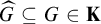 ,
$\widehat {G}\in \mathbf {K}$
,
$\widehat {G}\in \mathbf {K}$
 , the online coloring game
$\Gamma (\mathbf {K},n)$
, the online coloring game
$\Gamma (\mathbf {K},n)$
 is an infinite game of two players I and II, with the following rules:
-
• At step $2s$
, I chooses some graph
$G_{s}\in \mathbf {K}$
such that
$G_{s-1}\subseteq G_{s}$
. -
• At step $2s+1$
, II defines a coloring
$c_{s}:G_{s}\to \{0,1,\dots ,n-1\}$
such that
$c_{s}\restriction G_{s-1}=c_{s-1}$
.




Player I wins if at some finite step player II is unable to define
$c_{s}$
 , and player II wins otherwise.
For our purposes, we will mainly be focused on the class of planar graphs. Evidently, if player II has a computable winning strategy in
$\Gamma (\mathbf {K},n)$
 , then any computable graph
$G\in \mathbf {K}$
, then any computable graph
$G\in \mathbf {K}$
 has a computable n-coloring. In fact, it was shown in [Reference Schmerl and Simpson19, Theorem 1.2] that in natural classes of graphs (whose definition we omit but which include planar graphs), the converse also holds. Schmerl also showed that if player I has a winning strategy, for
$\Gamma (\mathbf {K},n)$
has a computable n-coloring. In fact, it was shown in [Reference Schmerl and Simpson19, Theorem 1.2] that in natural classes of graphs (whose definition we omit but which include planar graphs), the converse also holds. Schmerl also showed that if player I has a winning strategy, for
$\Gamma (\mathbf {K},n)$
 then
${\mathtt {RCA}_{0}}+\neg {{\mathtt {WKL}}}$
then
${\mathtt {RCA}_{0}}+\neg {{\mathtt {WKL}}}$
 suffices to produce a graph
$G\in \mathbf {K}$
suffices to produce a graph
$G\in \mathbf {K}$
 that is not n-colorable [Reference Schmerl and Simpson19, Theorem 2.1]. From the proof of [Reference Bean1, Theorem 2], one may easily extract a winning strategy for player I with
$\mathbf {K}$
that is not n-colorable [Reference Schmerl and Simpson19, Theorem 2.1]. From the proof of [Reference Bean1, Theorem 2], one may easily extract a winning strategy for player I with
$\mathbf {K}$
 as the class of planar graphs, thus implying that for any n,
${\mathtt {RCA}_{0}}+{\mathtt {COL}}(n)\,\vdash\, {{\mathtt {WKL}}}$
as the class of planar graphs, thus implying that for any n,
${\mathtt {RCA}_{0}}+{\mathtt {COL}}(n)\,\vdash\, {{\mathtt {WKL}}}$
 . With some slight modifications (see, for instance, Theorem 2.25), the graph constructed by Bean can be made both connected and such that it has a computable plane diagram, which further allows us to conclude that
${\mathtt {RCA}_{0}}+{\mathtt {ConnCOL}}(n)\,\vdash\, {{\mathtt {WKL}}}$
. With some slight modifications (see, for instance, Theorem 2.25), the graph constructed by Bean can be made both connected and such that it has a computable plane diagram, which further allows us to conclude that
${\mathtt {RCA}_{0}}+{\mathtt {ConnCOL}}(n)\,\vdash\, {{\mathtt {WKL}}}$
 and
${\mathtt {RCA}_{0}}+{\mathtt {COL}}^{*}(n)\,\vdash\, {{\mathtt {WKL}}}$
and
${\mathtt {RCA}_{0}}+{\mathtt {COL}}^{*}(n)\,\vdash\, {{\mathtt {WKL}}}$
 (see also [Reference Schmerl and Simpson19, Theorem 2]).
However, recall that the aim of this article is to study the ‘least level of non-uniformity’ required to obtain a reversal of the coloring principles for planar graphs. As such, we provide an alternative proof of some of Bean’s results, but with a focus on making the ‘gadgets’ more efficient. Whilst the proofs that follow will not be written explicitly in terms of games
$\Gamma (\mathbf {K},n)$
 , we are at least intuitively, attempting to find winning strategies for player I for various
$\mathbf {K}$
, we are at least intuitively, attempting to find winning strategies for player I for various
$\mathbf {K}$
 and n.
Whilst the following theorem is implied by the results of Bean and Schmerl, we include a proof of it as the graphs we construct are in some sense more ‘efficient’. In particular, the graphs constructed here will be helpful in obtaining various non-reductions later in Section 3.
Theorem 2.7 [Reference Bean1]
For any
$n\in {\mathbb {N}}$
 ,
${\mathtt {RCA}_{0}}\not \!\,\vdash\, {\mathtt {COL}}(n)$
,
${\mathtt {RCA}_{0}}\not \!\,\vdash\, {\mathtt {COL}}(n)$
 .
.
Proof. We first construct a planar computable graph that does not have a computable
$4$
 -coloring. Let
$\{\varphi _{e}\}_{e\in {\mathbb {N}}}$
-coloring. Let
$\{\varphi _{e}\}_{e\in {\mathbb {N}}}$
 be the standard listing of the partial computable functions from
${\mathbb {N}}$
be the standard listing of the partial computable functions from
${\mathbb {N}}$
 to
$\{0,1,2,3\}$
to
$\{0,1,2,3\}$
 . We construct a graph
$G=\langle V,E\rangle $
. We construct a graph
$G=\langle V,E\rangle $
 satisfying the following requirement for each
$e\in {\mathbb {N}}$
satisfying the following requirement for each
$e\in {\mathbb {N}}$
 .
.

We build G in stages, and say that a requirement
$R_{e}$
 is met when it has found some witness
$v_{e}^{*}$
is met when it has found some witness
$v_{e}^{*}$
 such that there is some v adjacent to
$v_{e}^{*}$
such that there is some v adjacent to
$v_{e}^{*}$
 and
$\varphi _{e}(v)=\varphi _{e}(v_{e}^{*}){\downarrow }$
and
$\varphi _{e}(v)=\varphi _{e}(v_{e}^{*}){\downarrow }$
 . In other words,
$\varphi _{e}$
. In other words,
$\varphi _{e}$
 fails to be a
$4$
fails to be a
$4$
 -coloring of G.
-
Stage $0$
: Enumerate a
$K_{4}$
graph into G and let the vertices of this
$K_{4}$
be denoted as
$v_{0,i}$
for each
$i<4$
. In addition to these vertices, also enumerate a single (temporarily) isolated vertex
$v_{0,4}$
into G. The vertices
$v_{0,j}$
for various j will be referred to as the
$0^{th}$
component of G. -
Stage $s>0$
: Begin the
$s^{th}$
component of G by enumerating five new vertices
$v_{s,j}$
for each
$j<5$
and connect
$v_{s,i}$
for each
$i<4$
as a
$K_{4}$
graph.For each $e<s$
, if
$\varphi _{e}(v_{e,j}){\downarrow }$
for all
$j<5$
and
$R_{e}$
has yet to act, then enumerate
$v_{e,5}$
into the
$e^{th}$
component and connect
$v_{e,5}$
to
$v_{e,4}$
and
$v_{e,i}$
for each
$i<4$
where
$\varphi _{e}(v_{e,i})\neq \varphi _{e}(v_{e,4})$
. Then declare
$v_{e,5}$
as the witness for
$R_{e}$
and proceed with the construction.





Observe that if some requirement
$R_{e}$
 never acts, then there must be some
$i<5$
never acts, then there must be some
$i<5$
 for which
$\varphi _{e}(v_{e,i})[s]{\uparrow }$
for which
$\varphi _{e}(v_{e,i})[s]{\uparrow }$
 at every stage s. Then
$\varphi _{e}$
at every stage s. Then
$\varphi _{e}$
 cannot possibly be total and thus
$R_{e}$
cannot possibly be total and thus
$R_{e}$
 is satisfied. Suppose then that there is some stage at which
$R_{e}$
is satisfied. Suppose then that there is some stage at which
$R_{e}$
 is discovered to be ready. Since there is no injury in the construction, (each requirement acts only on the component reserved for it), then
$R_{e}$
is discovered to be ready. Since there is no injury in the construction, (each requirement acts only on the component reserved for it), then
$R_{e}$
 must act at some stage s. When it does, recall that
$v_{e,5}$
must act at some stage s. When it does, recall that
$v_{e,5}$
 is then enumerated into the
$e^{th}$
is then enumerated into the
$e^{th}$
 component and connected with vertices
$v_{e,4}$
component and connected with vertices
$v_{e,4}$
 and
$v_{e,i}$
and
$v_{e,i}$
 for each
$i<4$
for each
$i<4$
 where
$\varphi _{e}(v_{e,i})\neq \varphi _{e}(v_{e,4})$
where
$\varphi _{e}(v_{e,i})\neq \varphi _{e}(v_{e,4})$
 . Then
$\varphi _{e}$
. Then
$\varphi _{e}$
 must fail as a
$4$
must fail as a
$4$
 -coloring as the neighbours of
$v_{e,5}$
-coloring as the neighbours of
$v_{e,5}$
 are colored four different colors.
The main idea was simply to wait until a potential coloring has used up all of its allowable colors in a certain configuration and then enumerating a new vertex connected to all the vertices colored with the allowable colors. Since
$K_{4}$
 is planar and must be colored with four colors, we can ensure that any potential
$4$
is planar and must be colored with four colors, we can ensure that any potential
$4$
 -coloring uses all four colors available to it. Evidently, we cannot simply enumerate a new vertex and connect it to all vertices currently in the
$K_{4}$
-coloring uses all four colors available to it. Evidently, we cannot simply enumerate a new vertex and connect it to all vertices currently in the
$K_{4}$
 otherwise the resulting graph is no longer planar. Thus we have an additional isolated vertex in each component to occupy the final color. It is not difficult to see that when the number of colors increases, the diagonalisation strategy will become more complex as it has to be able to get any potential coloring to commit to more colors. However, since every planar graph is
$4$
otherwise the resulting graph is no longer planar. Thus we have an additional isolated vertex in each component to occupy the final color. It is not difficult to see that when the number of colors increases, the diagonalisation strategy will become more complex as it has to be able to get any potential coloring to commit to more colors. However, since every planar graph is
$4$
 -colorable, it is evident that each component should become ‘layered’ in some way.
The general gadget will be as follows. Start by enumerating sufficiently many
$K_{4}$
 graphs. By pigeonhole principle, there will be at least two, say
$K_{4}^{0},K_{4}^{1}$
graphs. By pigeonhole principle, there will be at least two, say
$K_{4}^{0},K_{4}^{1}$
 , that are colored the same four colors. Now connect a new vertex
$\blacktriangle $
, that are colored the same four colors. Now connect a new vertex
$\blacktriangle $
 to two vertices each from
$K_{4}^{0}$
to two vertices each from
$K_{4}^{0}$
 and
$K_{4}^{1}$
and
$K_{4}^{1}$
 all of different colors. As shown in Figure 2, this is still a planar graph. Furthermore,
$\blacktriangle $
all of different colors. As shown in Figure 2, this is still a planar graph. Furthermore,
$\blacktriangle $
 cannot be colored any of the four colors used to color
$K_{4}^{0},K_{4}^{1}$
cannot be colored any of the four colors used to color
$K_{4}^{0},K_{4}^{1}$
 . We shall refer to the configuration in Figure 2 as
$W_{1}$
. We shall refer to the configuration in Figure 2 as
$W_{1}$
 and
$\blacktriangle $
and
$\blacktriangle $
 as the special vertex of
$W_{1}$
as the special vertex of
$W_{1}$
 .
.
$W_{1}$
 .
.

We refer the reader to Figure 3 for the illustration of the general gadget. To construct
$W_{n+1}$
 , start by enumerating a large number of
$K_{4}$
, start by enumerating a large number of
$K_{4}$
 graphs and wait for the coloring c, to converge on these graphs. Once it does, there must be sufficiently many
$K_{4}$
graphs and wait for the coloring c, to converge on these graphs. Once it does, there must be sufficiently many
$K_{4}$
 graphs all colored the same four colors, which we may assume to be
$0,1,2,3$
graphs all colored the same four colors, which we may assume to be
$0,1,2,3$
 . Then extend the
$K_{4}$
. Then extend the
$K_{4}$
 graphs (in the sense of Definition 2.5) into
$W_{1}$
graphs (in the sense of Definition 2.5) into
$W_{1}$
 graphs by pairing them up and enumerating the special vertices.
Notation 2.8. Let
$l\leq 4$
 and
$i\in {\mathbb {N}}$
and
$i\in {\mathbb {N}}$
 be given. We write
$K_{l}(W_{i})$
be given. We write
$K_{l}(W_{i})$
 to denote l many
$W_{i}$
to denote l many
$W_{i}$
 graphs, where the special vertices (to be defined shortly for
$i>1$
graphs, where the special vertices (to be defined shortly for
$i>1$
 , also see Figure 3) of the
$W_{i}$
, also see Figure 3) of the
$W_{i}$
 graphs are connected as a
$K_{l}$
graphs are connected as a
$K_{l}$
 graph. For convenience, we also use
$W_{0}$
graph. For convenience, we also use
$W_{0}$
 to denote a single vertex;
$K_{4}(W_{0})$
to denote a single vertex;
$K_{4}(W_{0})$
 is isomorphic to
$K_{4}$
is isomorphic to
$K_{4}$
 .
.
$W_{n+1}$
 .
.

Figure 3. Long description
A horizontal sequence of six graph structures is arranged across the top. From left to right, the first two structures are simple tetrahedral graphs with four solid black nodes each. The next two structures are larger triangular clusters where each of the four nodes is labeled W sub 1. An ellipsis indicates a continuation of the pattern. The final two structures are triangular clusters where each of the four nodes is labeled W sub n. Each triangular cluster consists of three outer nodes forming a triangle with a fourth node at the center, all interconnected. From the bottom-most nodes of every cluster, curved and straight lines descend to converge at a single solid black triangular vertex located at the bottom center of the diagram.
In addition, extend the resulting
$W_{1}$
 graphs into
$K_{4}(W_{1})$
graphs into
$K_{4}(W_{1})$
 graphs by connecting the special vertices of four
$W_{1}$
graphs by connecting the special vertices of four
$W_{1}$
 graphs as a
$K_{4}$
graphs as a
$K_{4}$
 . The idea here is that since the special vertex of each
$W_{1}$
. The idea here is that since the special vertex of each
$W_{1}$
 cannot be colored any of
$0,1,2,3$
cannot be colored any of
$0,1,2,3$
 , then the new
$K_{4}(W_{1})$
, then the new
$K_{4}(W_{1})$
 configuration forces the coloring to use the next four colors.
In general, once the coloring has converged on the vertices of all the
$K_{4}(W_{n})$
 graphs, we extend it to
$W_{n+1}$
graphs, we extend it to
$W_{n+1}$
 by enumerating a special vertex
$\blacktriangle $
by enumerating a special vertex
$\blacktriangle $
 and connecting it to two copies each of
$K_{4},K_{4}(W_{1}),\dots ,K_{4}(W_{n})$
and connecting it to two copies each of
$K_{4},K_{4}(W_{1}),\dots ,K_{4}(W_{n})$
 as shown in Figure 3. We may assume that each pair of
$K_{4}(W_{i})$
as shown in Figure 3. We may assume that each pair of
$K_{4}(W_{i})$
 is colored with
$4i,4i+1,4i+2$
is colored with
$4i,4i+1,4i+2$
 , and
$4i+3$
, and
$4i+3$
 (by pigeonhole principle). Then by connecting
$\blacktriangle $
(by pigeonhole principle). Then by connecting
$\blacktriangle $
 the special vertices of these various
$K_{4}(W_{i})$
the special vertices of these various
$K_{4}(W_{i})$
 , each colored
$4i,4i+1,4i+2,4i+3$
, each colored
$4i,4i+1,4i+2,4i+3$
 , the coloring cannot use any of the first
$4n$
, the coloring cannot use any of the first
$4n$
 many colors to color
$\blacktriangle $
many colors to color
$\blacktriangle $
 . Now take four copies of
$W_{n+1}$
. Now take four copies of
$W_{n+1}$
 which are colored the same
$4n$
which are colored the same
$4n$
 colors (except the special vertex) and connect the special vertices as a
$K_{4}$
colors (except the special vertex) and connect the special vertices as a
$K_{4}$
 graph to form
$K_{4}(W_{n+1})$
graph to form
$K_{4}(W_{n+1})$
 . Evidently, for a fixed computable k-coloring
$\varphi $
. Evidently, for a fixed computable k-coloring
$\varphi $
 ,
$W_{n}$
,
$W_{n}$
 cannot be colored by
$\varphi $
cannot be colored by
$\varphi $
 for any
$n\geq \lceil k/4\rceil $
for any
$n\geq \lceil k/4\rceil $
 .
.
Notation 2.9. Since
$W_{n}$
 will generally be defined based on some coloring, to emphasise this, we will write the function used to define
$W_{n}$
will generally be defined based on some coloring, to emphasise this, we will write the function used to define
$W_{n}$
 in the superscript. In particular, if
$\varphi $
in the superscript. In particular, if
$\varphi $
 is a k-coloring, then for any
$n\geq \lceil k/4\rceil $
is a k-coloring, then for any
$n\geq \lceil k/4\rceil $
 ,
$W_{n}^{\varphi }$
,
$W_{n}^{\varphi }$
 cannot be colored by
$\varphi $
cannot be colored by
$\varphi $
 .
.
Let some
$n\geq 4$
 be given and let
$\{\varphi _{e}\}_{e\in {\mathbb {N}}}$
be given and let
$\{\varphi _{e}\}_{e\in {\mathbb {N}}}$
 be a listing of the computable functions
$\varphi _{e}:{\mathbb {N}}\to \{0,1,\dots ,n-1\}$
be a listing of the computable functions
$\varphi _{e}:{\mathbb {N}}\to \{0,1,\dots ,n-1\}$
 . Once again we aim to construct a graph G satisfying the conditions below:

The graph will be constructed in components where each component aims to satisfy a single
$R_{e}$
 . The action on the
$e^{th}$
. The action on the
$e^{th}$
 component will depend solely on the behaviour of
$\varphi _{e}$
component will depend solely on the behaviour of
$\varphi _{e}$
 .
.
Fix some
$e\in {\mathbb {N}}$
 . In the
$e^{th}$
. In the
$e^{th}$
 component, we aim to construct a
$W_{m}^{\varphi _{e}}$
component, we aim to construct a
$W_{m}^{\varphi _{e}}$
 where m is the least such that
$m\geq \lceil n/4\rceil $
where m is the least such that
$m\geq \lceil n/4\rceil $
 . Since we know exactly how many
$K_{4},K_{4}(W_{1}),\dots ,K_{4}(W_{m-1})$
. Since we know exactly how many
$K_{4},K_{4}(W_{1}),\dots ,K_{4}(W_{m-1})$
 are needed, the required starting amount of
$K_{4}$
are needed, the required starting amount of
$K_{4}$
 graphs can be found recursively. Begin by enumerating a sufficiently large number of
$K_{4}$
graphs can be found recursively. Begin by enumerating a sufficiently large number of
$K_{4}$
 graphs into the
$e^{th}$
graphs into the
$e^{th}$
 component. Proceed to construct
$W_{m}^{\varphi _{e}}$
component. Proceed to construct
$W_{m}^{\varphi _{e}}$
 as described previously; wait for
$\varphi _{e}$
as described previously; wait for
$\varphi _{e}$
 to converge on the vertices in
$K_{4}(W_{i}^{\varphi _{e}})$
to converge on the vertices in
$K_{4}(W_{i}^{\varphi _{e}})$
 before extending them to
$W_{i+1}^{\varphi _{e}}$
before extending them to
$W_{i+1}^{\varphi _{e}}$
 .
.
If
$\varphi _{e}$
 is total, it must converge on every vertex within the
$e^{th}$
is total, it must converge on every vertex within the
$e^{th}$
 component. Then we must succeed in constructing
$W_{m}^{\varphi _{e}}$
component. Then we must succeed in constructing
$W_{m}^{\varphi _{e}}$
 . However, in order for
$\varphi _{e}$
. However, in order for
$\varphi _{e}$
 to successfully color
$W_{m}^{\varphi _{e}}$
to successfully color
$W_{m}^{\varphi _{e}}$
 ,
$4m+1$
,
$4m+1$
 colors are needed. By choice of m, we obtain that
$4m+1\geq n+1>n$
colors are needed. By choice of m, we obtain that
$4m+1\geq n+1>n$
 ;
$\varphi _{e}$
;
$\varphi _{e}$
 cannot be a computable n-coloring.
2.2 Reducing
${{\mathtt {WKL}}}$
to the four color theorem

First we observe that for any
$n\geq 4,$


It follows immediately from the definitions that
${\mathtt {ConnCOL}}(n),{\mathtt {COL}}^{*}(n){\leq _{\mathsf {sW}}}{\mathtt {COL}}(n)$
 , simply by ‘forgetting’ connectedness or the plane diagram, respectively. To obtain that
${\mathtt {COL}}(n){\leq _{\mathsf {sW}}}{{\mathtt {WKL}}}$
, simply by ‘forgetting’ connectedness or the plane diagram, respectively. To obtain that
${\mathtt {COL}}(n){\leq _{\mathsf {sW}}}{{\mathtt {WKL}}}$
 , one simply needs to consider the tree of all possible n-colorings of a given graph, which is clearly a bounded tree. By applying the classical De-Bruijn–Erdős theorem, such a tree must have a path, and
${{\mathtt {WKL}}}$
, one simply needs to consider the tree of all possible n-colorings of a given graph, which is clearly a bounded tree. By applying the classical De-Bruijn–Erdős theorem, such a tree must have a path, and
${{\mathtt {WKL}}}$
 suffices to produce one such path. Note that this does not imply that for each
$n\geq 4 \, {{\mathtt {WKL}}}_{0}\,\vdash\, {\mathtt {COL}}(n)$
suffices to produce one such path. Note that this does not imply that for each
$n\geq 4 \, {{\mathtt {WKL}}}_{0}\,\vdash\, {\mathtt {COL}}(n)$
 .
.
To show that
${\mathtt {COL}}(4)$
 and
${{\mathtt {WKL}}}$
and
${{\mathtt {WKL}}}$
 are equivalent over
${\mathtt {RCA}_{0}}$
are equivalent over
${\mathtt {RCA}_{0}}$
 , one evidently needs to verify that
${{\mathtt {WKL}}}_{0}\,\vdash\, {\mathtt {COL}}(4)$
, one evidently needs to verify that
${{\mathtt {WKL}}}_{0}\,\vdash\, {\mathtt {COL}}(4)$
 . The most natural way to approach this would be to first show that
${\mathtt {RCA}_{0}}$
. The most natural way to approach this would be to first show that
${\mathtt {RCA}_{0}}$
 proves that every finite planar graph is
$4$
proves that every finite planar graph is
$4$
 -colorable, and then extending these finite colorings with the De-Bruijn–Erdős theorem (restricted to countable graphs). While we conjecture that the finitary four color theorem should hold in
${\mathtt {RCA}_{0}}$
-colorable, and then extending these finite colorings with the De-Bruijn–Erdős theorem (restricted to countable graphs). While we conjecture that the finitary four color theorem should hold in
${\mathtt {RCA}_{0}}$
 , we leave the verification open. Nonetheless, we show that each of
${\mathtt {COL}}(4),{\mathtt {ConnCOL}}(4)$
, we leave the verification open. Nonetheless, we show that each of
${\mathtt {COL}}(4),{\mathtt {ConnCOL}}(4)$
 , and
${\mathtt {COL}}^{*}(4)$
, and
${\mathtt {COL}}^{*}(4)$
 may be ‘reversed uniformly’ over
${\mathtt {RCA}_{0}}$
may be ‘reversed uniformly’ over
${\mathtt {RCA}_{0}}$
 to
${{\mathtt {WKL}}}$
to
${{\mathtt {WKL}}}$
 .
.
Theorem 2.10.
${{\mathtt {WKL}}}{\leq _{\mathsf {sW}}}{\mathtt {COL}}(4)$
 .
.
Proof. Let
$T\subseteq 2^{<{\mathbb {N}}}$
 be an infinite tree. We construct a countable planar graph,
$G=\langle V,E\rangle $
be an infinite tree. We construct a countable planar graph,
$G=\langle V,E\rangle $
 in stages as follows. An illustration of G can be found in Figure 4. The vertex set V will contain the following type of vertices:
-
• $W=\{w_{\tau },v_{\tau }\mid \tau \in 2^{<{\mathbb {N}}}\}.$
-
• $F=\{f_{\tau }\mid \tau \in 2^{<{\mathbb {N}}}\}$
. -
• $N=\{n_{\tau }\mid \tau \in 2^{<{\mathbb {N}}}\}$
. -
• A, some infinite set of vertices to be used in the construction.



Reducing
${{\mathtt {WKL}}}$
 to
${\mathtt {COL}}(4)$
to
${\mathtt {COL}}(4)$
 .
.

Figure 4. Long description
The diagram consists of two panels.
Left panel titled The tau-th, tau 0-th and tau 1-th component.
At the bottom is node n sub tau. Above it is a central node f sub tau flanked by v sub tau and w sub tau, forming a small diamond shape connected to n sub tau. This structure is enclosed in a larger triangle with vertices n sub tau, n sub tau 0, and n sub tau 1.
Above n sub tau 0 is a second hierarchical level. It features a base node n sub tau 0 connected to a central node f sub tau 0, flanked by two smaller nodes v sub tau 0 and w sub tau 0. This is enclosed in a triangle with top vertices n sub tau 00 and n sub tau 01.
Above n sub tau 1 is a third hierarchical level. It features a base node n sub tau 1 connected to a central node f sub tau 1, flanked by two smaller nodes v sub tau 1 and w sub tau 1. This is enclosed in a triangle with top vertices n sub tau 10 and n sub tau 11.
Right panel titled Acting in the sigma super th component.
At the bottom is node n sub sigma. Lines radiate upward to a wide top edge defined by nodes n sub sigma 0 on the left and n sub sigma 1 on the right.
In the center of the top edge is node f sub sigma. Below f sub sigma are nodes v sub sigma and w sub sigma.
To the left of f sub sigma, two triangular markers are placed on the connecting lines. To the right of f sub sigma, one triangular marker is placed on a connecting line.
All nodes are connected by straight lines forming a complex mesh of nested triangles.
-
Stage $0$
: Enumerate
$f_{\epsilon },w_{\epsilon },v_{\epsilon },n_{\epsilon },n_{0}$
, and
$n_{1}$
. Connect them as shown in Figure 4 (take
$\tau =\epsilon $
). -
Stage $s>0$
: For each
$\tau \in 2^{<{\mathbb {N}}}$
of length s, enumerate the vertices
$n_{\tau 0},n_{\tau 1},f_{\tau },v_{\tau }$
, and
$w_{\tau }$
, and connect them as shown in Figure 4. We shall refer to this as the
$\tau $
-th component of the graph.We say that the $\sigma $
-th component has acted when a vertex from A has been enumerated and connected to the vertices in the
$\sigma $
-th component. We once again refer the reader to Figure 4 for an illustration, where the vertices from A are denoted by the triangular vertices. Furthermore, once the
$\sigma $
-th component has acted, we also say that it has chosen
$\sigma x$
if there is only one vertex from A between
$w_{\sigma }$
or
$v_{\sigma }$
and
$n_{\sigma x}$
. As an example, the
$\sigma $
-th component in Figure 4 has chosen
$\sigma 1$
.For convenience, we assume that at each stage, we compute the value of $T(\tau )$
for the next
$\tau $
. If at stage s,
$\tau x$
is found to be in the complement, then pick the maximal prefix
$\sigma \subseteq \tau $
such that the
$\sigma $
-th component has yet to act. Let y be such that
$\sigma y\subseteq \tau x$
and act for the
$\sigma $
-th component, choosing
$\sigma ^{\frown }(1-y)$
.







Since each (diagonalisation) component is clearly planar and they are connected as shown in Figure 4, the graph as defined above is connected and planar. Applying Proposition 2.2 allows us to conclude that whenever some
$\tau x$
 is discovered to be in the complement of T, the maximal prefix
$\sigma \subseteq \tau $
is discovered to be in the complement of T, the maximal prefix
$\sigma \subseteq \tau $
 that has yet to act can always be found. Furthermore, if the
$\sigma $
that has yet to act can always be found. Furthermore, if the
$\sigma $
 -th component acts and chooses
$\sigma ^{\frown }(1-y)$
-th component acts and chooses
$\sigma ^{\frown }(1-y)$
 , then the subtree above
$\sigma y$
, then the subtree above
$\sigma y$
 is finite.
By
${\mathtt {COL}}(4)$
 , there is a coloring
$c:V\to \{0,1,2,3\}$
, there is a coloring
$c:V\to \{0,1,2,3\}$
 of G. We extract a path h through T using c as follows. Let
$\tau _{i}=h\restriction i$
of G. We extract a path h through T using c as follows. Let
$\tau _{i}=h\restriction i$
 .
.
-
• If $c(v_{\tau _{i}})=c(n_{\tau _{i}0})$
, then let
$h(i)=0$
. -
• Otherwise, let $h(i)=1$
.



We proceed by induction on i to verify that
$\tau _{i}\in T$
 for every i. Base case is trivial since
$\tau _{0}=\epsilon $
for every i. Base case is trivial since
$\tau _{0}=\epsilon $
 . Suppose inductively that
$\tau _{i}\in T$
. Suppose inductively that
$\tau _{i}\in T$
 and consider the following cases:
-
Case 1: $h(i)=0$
. If the
$\tau _{i}$
-th component never acts, since
$\tau _{i}\in T$
, then both subtrees extending
$\tau _{i}0$
and
$\tau _{i}1$
must be infinite (by Proposition 2.3). We may thus assume for a contradiction that the
$\tau _{i}$
-th component has acted and chooses
$\tau _{i}1$
; there are two vertices from A between
$v_{\tau _{i}}$
and
$n_{\tau _{i}0}$
. However, by definition of h, we also have that
$c(v_{\tau _{i}})=c(n_{\tau _{i}0})$
. This leads to a contradiction since c has only one color to color the two adjacent vertices from A between
$v_{\tau _{i}}$
and
$n_{\tau _{i}0}$
. -
Case 2: $h(i)=1$
. Once again, we may assume for a contradiction that the
$\tau _{i}$
-th component acts and chooses
$\tau _{i}0$
. In other words, there is exactly one vertex from A between
$v_{\tau _{i}}$
and
$n_{\tau _{i}0}$
(the
$\tau $
-th component chooses
$\tau _{i}0$
). Since
$h(i)=1$
, then
$c(v_{\tau _{i}})\neq c(n_{\tau _{i}0})$
; the vertex from A between
$v_{\tau _{i}}$
and
$n_{\tau _{i}0}$
is connected to four vertices all colored different colors by c. Therefore, c cannot be a valid coloring of G.








Thus, h must be a path through T. Since h can be computed solely from c, we obtain that
${{\mathtt {WKL}}}{\leq _{\mathsf {sW}}}{\mathtt {COL}}(4)$
 as desired.
Remark 2.11. Notice that the graph G constructed in the proof of the theorem above has a T-computable plane diagram and is also connected. Therefore, the principles
${\mathtt {ConnCOL}}(4)$
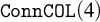 and
${\mathtt {COL}}^{*}(4)$
and
${\mathtt {COL}}^{*}(4)$
 are also able to produce a
$4$
are also able to produce a
$4$
 -coloring of G. Additionally, the proof above may be easily carried out in
${\mathtt {RCA}_{0}}$
-coloring of G. Additionally, the proof above may be easily carried out in
${\mathtt {RCA}_{0}}$
 , and thus, we also obtain the earlier results for
$n=4$
, and thus, we also obtain the earlier results for
$n=4$
 by Bean and Schmerl as a corollary.
Corollary 2.12.
${\mathtt {RCA}_{0}}+\mathcal {C}\,\,\vdash\, {{\mathtt {WKL}}}$
 where
$\mathcal {C}$
where
$\mathcal {C}$
 is any of
${\mathtt {COL}}(4),{\mathtt {ConnCOL}}(4)$
is any of
${\mathtt {COL}}(4),{\mathtt {ConnCOL}}(4)$
 , and
${\mathtt {COL}}^{*}(4)$
, and
${\mathtt {COL}}^{*}(4)$
 .
.
2.3 Reducing
${\mathtt {DNR}}(k)$
to
${\mathtt {COL}}(7)$


Unlike the case for four colors, it is not difficult to verify that for any
$n>4\, {\mathtt {RCA}_{0}}$
 proves that every finite planar graph is n-colorable. (See, e.g., the proof given by [Reference Chartrand, Lesniak and Zhang4, Theorem 9.1].) Applying this with the fact that
${{\mathtt {WKL}}}$
proves that every finite planar graph is n-colorable. (See, e.g., the proof given by [Reference Chartrand, Lesniak and Zhang4, Theorem 9.1].) Applying this with the fact that
${{\mathtt {WKL}}}$
 and the De-Bruijn–Erdős theorem are equivalent over
${\mathtt {RCA}_{0}}$
and the De-Bruijn–Erdős theorem are equivalent over
${\mathtt {RCA}_{0}}$
 [Reference Hirst11] together with Theorem 1.1 allows us to conclude that for any
$n>4$
[Reference Hirst11] together with Theorem 1.1 allows us to conclude that for any
$n>4$
 ,
${\mathtt {COL}}(n)$
,
${\mathtt {COL}}(n)$
 and
${{\mathtt {WKL}}}$
and
${{\mathtt {WKL}}}$
 are equivalent over
${\mathtt {RCA}_{0}}$
are equivalent over
${\mathtt {RCA}_{0}}$
 .
.
As discussed in Section 2.1, allowing the coloring access to more than four colors adds some level of complexity to the required proof. In particular, the proof as presented for Theorem 2.10 will not work if the principle is
${\mathtt {COL}}(5)$
 . The gadget used to obtain
${{\mathtt {WKL}}}{\leq _{\mathsf {W}}}{\mathtt {COL}}(4)$
. The gadget used to obtain
${{\mathtt {WKL}}}{\leq _{\mathsf {W}}}{\mathtt {COL}}(4)$
 mainly uses the property that four colors are required to color
$K_{4}$
mainly uses the property that four colors are required to color
$K_{4}$
 . However, a graph that requires five colors to color is obviously not going to be planar. At least intuitively, this seems to suggest that for
$n\geq 5$
. However, a graph that requires five colors to color is obviously not going to be planar. At least intuitively, this seems to suggest that for
$n\geq 5$
 , we no longer have that
${{\mathtt {WKL}}}{\leq _{\mathsf {W}}}{\mathtt {COL}}(n),{\mathtt {ConnCOL}}(n)$
, we no longer have that
${{\mathtt {WKL}}}{\leq _{\mathsf {W}}}{\mathtt {COL}}(n),{\mathtt {ConnCOL}}(n)$
 , and
${\mathtt {COL}}^{*}(n)$
, and
${\mathtt {COL}}^{*}(n)$
 . As mentioned earlier, we shall show this formally for
$n\geq 7$
. As mentioned earlier, we shall show this formally for
$n\geq 7$
 (see Theorems 3.5 and 3.13), but leave the cases for
$n=5,6$
(see Theorems 3.5 and 3.13), but leave the cases for
$n=5,6$
 open.
open.
To investigate the level of non-uniformity required in reversing the coloring principles to
${{\mathtt {WKL}}}$
 over
${\mathtt {RCA}_{0}}$
over
${\mathtt {RCA}_{0}}$
 , we attempt to reduce
${\mathtt {DNR}}(k)$
, we attempt to reduce
${\mathtt {DNR}}(k)$
 (to be defined shortly) principles to the various coloring principles. This is motivated by the fact that these principles have been used to study graph colorings in reverse mathematics [Reference Dorais, Hirst and Shafer8] (similar ideas can also be found in [Reference Schmerl18, Reference Schmerl and Simpson19]).
Definition 2.13 (
${\mathtt {RCA}_{0}}$
)

Let
$\{\varphi _{x}\}_{x\in {\mathbb {N}}}$
 be a standard listing of the partial computable functions.
-
• ${\mathtt {DNR}}$
is the principle: $$ \begin{align*}\forall f:{\mathbb{N}}\to{\mathbb{N}},\,\exists g:{\mathbb{N}}\to{\mathbb{N}}\text{ such that }\forall x,\,g(x)\neq\varphi_{x}^{f}(x). \end{align*} $$
-
• ${\mathtt {DNR}}(k)$
is the principle: $$ \begin{align*}\forall f:{\mathbb{N}}\to{\mathbb{N}},\,\exists g:{\mathbb{N}}\to\{0,1,2,\dots,k-1\}\text{ such that }\forall x,g(x)\neq\varphi_{x}^{f}(x). \end{align*} $$


It is known that
${{\mathtt {WKL}}}$
 and
${\mathtt {DNR}}(2)$
and
${\mathtt {DNR}}(2)$
 are equivalent (uniformly) over
${\mathtt {RCA}_{0}}$
are equivalent (uniformly) over
${\mathtt {RCA}_{0}}$
 [Reference Jockush13]. It is also not difficult to see that
${{\mathtt {WKL}}}\equiv _{\mathsf {W}}{\mathtt {DNR}}(2)$
[Reference Jockush13]. It is also not difficult to see that
${{\mathtt {WKL}}}\equiv _{\mathsf {W}}{\mathtt {DNR}}(2)$
 and that for any
$k\geq 2$
and that for any
$k\geq 2$
 , we have that
${\mathtt {DNR}}{\leq _{\mathsf {W}}}{\mathtt {DNR}}(k+1){\leq _{\mathsf {W}}}{\mathtt {DNR}}(k)$
, we have that
${\mathtt {DNR}}{\leq _{\mathsf {W}}}{\mathtt {DNR}}(k+1){\leq _{\mathsf {W}}}{\mathtt {DNR}}(k)$
 . With the work of Jockush [Reference Jockush13], we further have that each of these reductions is strict. In the remainder of the section, we attempt to find the least k for which
${\mathtt {DNR}}(k){\leq _{\mathsf {W}}}\mathcal {C}$
. With the work of Jockush [Reference Jockush13], we further have that each of these reductions is strict. In the remainder of the section, we attempt to find the least k for which
${\mathtt {DNR}}(k){\leq _{\mathsf {W}}}\mathcal {C}$
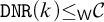 for the various coloring principles
$\mathcal {C}$
for the various coloring principles
$\mathcal {C}$
 , and hence also provides an upper bound for the level of non-uniformity required for reversal to
${{\mathtt {WKL}}}$
, and hence also provides an upper bound for the level of non-uniformity required for reversal to
${{\mathtt {WKL}}}$
 over
${\mathtt {RCA}_{0}}$
over
${\mathtt {RCA}_{0}}$
 . (See Figure 5 for a summary of the results.)
Theorem 2.14.
${\mathtt {DNR}}(3){\leq _{\mathsf {sW}}}{\mathtt {COL}}^{*}(5)$
 .
.
Hierarchy of principles: Each arrow and crossed arrow in the diagram from P to Q represents
$P{\leq _{\mathsf {sW}}} Q$
 and
$P\not \!\!{\leq _{\mathsf {W}}} Q,$
and
$P\not \!\!{\leq _{\mathsf {W}}} Q,$
 respectively.

Proof. Fix some
$f:{\mathbb {N}}\to {\mathbb {N}}$
 , and let
$\left \{\varphi _{e}^{f}\right \}_{e\in {\mathbb {N}}}$
, and let
$\left \{\varphi _{e}^{f}\right \}_{e\in {\mathbb {N}}}$
 be the standard listing of the f-computable functions. G will consist of components, each consisting of six
$K_{3}$
be the standard listing of the f-computable functions. G will consist of components, each consisting of six
$K_{3}$
 graphs originally, labelled
$K_{3}^{j}$
graphs originally, labelled
$K_{3}^{j}$
 for each
$j<6$
for each
$j<6$
 . At each stage s, check if
$\varphi _{e}^{f}(e)[s]{\downarrow }$
. At each stage s, check if
$\varphi _{e}^{f}(e)[s]{\downarrow }$
 . If
$\varphi _{e}^{f}(e)[s]{\uparrow }$
. If
$\varphi _{e}^{f}(e)[s]{\uparrow }$
 , then do nothing. Otherwise, enumerate vertices into the
$e^{th}$
, then do nothing. Otherwise, enumerate vertices into the
$e^{th}$
 component and connect them as illustrated in Figure 6, where
$\circ $
component and connect them as illustrated in Figure 6, where
$\circ $
 represents the newly enumerated vertices, and the numbered
$K_{3}$
represents the newly enumerated vertices, and the numbered
$K_{3}$
 graphs correspond to
$K_{3}^{j}$
graphs correspond to
$K_{3}^{j}$
 for
$j<6$
for
$j<6$
 .
.
The gadget for Theorem 2.14.

Figure 6. Long description
A four-panel diagram illustrating graph gadgets. Each panel contains six triangular components labeled 0 through 5, with 0, 1, and 2 on the bottom row and 3, 4, and 5 on the top row. Each triangle has three black nodes.
* Top-left panel: Condition is If phi sub e super f of e diverges or phi sub e super f of e converges to a value greater than 2. The six triangles are disconnected from each other.
* Top-right panel: Condition is If phi sub e super f of e converges to 0. The top three triangles are connected to a central horizontal structure of three white nodes, and the bottom three triangles are connected to a separate identical structure below it.
* Bottom-left panel: Condition is If phi sub e super f of e converges to 1. All top triangles are connected to a single white node, which is connected by a vertical edge to a second white node that connects to all bottom triangles.
* Bottom-right panel: Condition is If phi sub e super f of e converges to 2. All six triangles are connected to a single central white node, creating a unified star-like structure.
G as constructed above is clearly planar, and has an f-computable planar drawing, and thus by
${\mathtt {COL}}^{*}(5)$
 has a
$5$
has a
$5$
 -coloring c. For convenience, in the
$e^{th}$
-coloring c. For convenience, in the
$e^{th}$
 component, define
$A_{e}=\{c(v)\mid v\in K_{3}^{j}\text { for }j<3\}$
component, define
$A_{e}=\{c(v)\mid v\in K_{3}^{j}\text { for }j<3\}$
 and
$B_{e}=\{c(v)\mid v\in K_{3}^{j}\text { for }3\leq j<6\}$
and
$B_{e}=\{c(v)\mid v\in K_{3}^{j}\text { for }3\leq j<6\}$
 . Then define g as follows:
-
• Define $g(e)=0$
if
$|A_{e}|=3$
or
$|B_{e}|=3$
.We now claim that if this is the case, $g(e)\neq \varphi _{e}^{f}(e)$
. Suppose otherwise, then
$\varphi _{e}^{f}(e)=g(e)=0$
, and hence it must be that one of the sets
$A_{e}$
or
$B_{e}$
has size
$3$
. Referring to Figure 6, observe that in either case, c cannot possibly extend to a
$5$
-coloring of the
$e^{th}$
component. -
• Define $g(e)=1$
, if
$A_{e}=B_{e}$
and
$|A_{e}|=|B_{e}|=4$
.Once again, we check that $g(e)\neq \varphi _{e}^{f}(e)$
. Suppose to the contrary that
$\varphi _{e}^{f}(e){\downarrow }=g(e)=1$
. Then the two new vertices
$v,w$
enumerated in this case cannot be colored by any of the four colors in
$A_{e},B_{e}$
. However, as v is also adjacent to w, c cannot color both
$v,w$
with the single remaining color. -
• Define $g(e)=2$
if both of the above cases do not hold.Assume for a contradiction that $\varphi _{e}^{f}(e)=g(e)=2$
, then a single vertex v must have been enumerated into the
$e^{th}$
component. Furthermore, this vertex is connected to all other vertices in the
$e^{th}$
component. But c is assumed to have already used up all five colors to color the original vertices in the
$e^{th}$
component, leaving it no color for v.


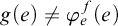




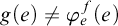






Thus g as defined above satisfies
${\mathtt {DNR}}(3)$
 and can be computed from c (a solution to the constructed instance G of
${\mathtt {COL}}^{*}(5)$
and can be computed from c (a solution to the constructed instance G of
${\mathtt {COL}}^{*}(5)$
 ). Therefore,
${\mathtt {DNR}}(3){\leq _{\mathsf {sW}}}{\mathtt {COL}}^{*}(5)$
). Therefore,
${\mathtt {DNR}}(3){\leq _{\mathsf {sW}}}{\mathtt {COL}}^{*}(5)$
 .
.
To obtain
${\mathtt {DNR}}(3){\leq _{\mathsf {sW}}}{\mathtt {ConnCOL}}(5)$
 , we simply need to modify the gadget in a way that makes it connected. For each
$K_{3}$
, we simply need to modify the gadget in a way that makes it connected. For each
$K_{3}$
 graph enumerated as the initial part of a gadget, we enumerate a single vertex and connect it to a vertex of the
$K_{3}$
graph enumerated as the initial part of a gadget, we enumerate a single vertex and connect it to a vertex of the
$K_{3}$
 . Now connect all of these new vertices as an infinite path. Observe that this results in a planar connected graph. As a result,
${\mathtt {ConnCOL}}(5)$
. Now connect all of these new vertices as an infinite path. Observe that this results in a planar connected graph. As a result,
${\mathtt {ConnCOL}}(5)$
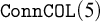 can therefore produce a
$5$
can therefore produce a
$5$
 -coloring of this new graph and g can be defined in the same way as before. We thus obtain the following as a corollary.
Theorem 2.15.
${\mathtt {DNR}}(3){\leq _{\mathsf {sW}}}{\mathtt {ConnCOL}}(5)$
 .
.
We now address the case for
$n=6$
 . The key ingredient in the proof for the case
$n=5$
. The key ingredient in the proof for the case
$n=5$
 was to have some base configuration that can be extended (recall Definition 2.5) into three different graphs with the following property. Any coloring of the extended graphs, when restricted back to the original configuration, results in different colorings. This allows us to successfully avoid the value of
$\varphi _{e}^{f}(e)$
was to have some base configuration that can be extended (recall Definition 2.5) into three different graphs with the following property. Any coloring of the extended graphs, when restricted back to the original configuration, results in different colorings. This allows us to successfully avoid the value of
$\varphi _{e}^{f}(e)$
 by considering the coloring of the base configuration. We adopt a similar idea for the remaining cases. For
${\mathtt {COL}}^{*}(6)$
by considering the coloring of the base configuration. We adopt a similar idea for the remaining cases. For
${\mathtt {COL}}^{*}(6)$
 , we use a base configuration that can be extended into four different graphs such that any coloring of the base configuration fails to extend to at least one of the four graph extensions. We specify the details below.
Theorem 2.16.
${\mathtt {DNR}}(4){\leq _{\mathsf {sW}}}{\mathtt {COL}}^{*}(6)$
 .
.
Proof. Fix some
$f:{\mathbb {N}}\to {\mathbb {N}}$
 , and let
$\left \{\varphi _{e}^{f}(e)\right \}_{e\in {\mathbb {N}}}$
, and let
$\left \{\varphi _{e}^{f}(e)\right \}_{e\in {\mathbb {N}}}$
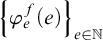 be a standard listing of the f-computable functions. Once again, G will be made up of components, each of which now contains 24
$K_{3}$
be a standard listing of the f-computable functions. Once again, G will be made up of components, each of which now contains 24
$K_{3}$
 graphs, denoted as
$K_{3}^{j}$
graphs, denoted as
$K_{3}^{j}$
 for each
$j<24$
for each
$j<24$
 .
.
At each stage s, do the following.
-
Stage s: Enumerate the new $s^{th}$
component by enumerating 24 new
$K_{3}$
graphs into G. For each
$e<s$
, which is not yet declared satisfied, do the following.-
• If $\varphi _{e}^{f}(e)[s]{\downarrow }=0$
, then enumerate 24 new vertices,
$v_{j}$
, for each
$j<24$
, into the
$e^{th}$
component. For each j, connect
$v_{j}$
to all vertices in
$K_{3}^{j}$
, and then for each
$i<6$
, connect the vertices
$v_{j}$
where
$4i\leq j<4(i+1)$
in a
$K_{4}$
graph. (See Figure 7 for an illustration; the labels of the
$K_{3}$
graphs correspond to j and the newly enumerated vertices are represented by
$\circ $
.)Figure 7The gadget for Theorem 2.16. We use ‘ $\cdots $
’ to replace the edges to avoid cluttering the diagram.Figure 7. Long description
The diagram consists of two panels, each with a logical statement at the top.
Left Panel: Labeled ‘If phi super f sub e (e) down-arrow = 0, then for each i < 6’. It shows a graph with four triangular clusters labeled K sub 3 super 4i+2, K sub 3 super 4i+3, K sub 3 super 4i+1, and K sub 3 super 4i. Three clusters on the left (top, middle, and bottom) converge toward two central white nodes. The middle cluster, K sub 3 super 4i+3, is nested within the structure. The rightmost cluster, K sub 3 super 4i, is connected to the central nodes via a horizontal bridge of two white nodes. Black dots represent vertices within the clusters, while white circles represent connecting nodes.
Right Panel: Labeled ‘If phi super f sub e (e) down-arrow = 1, then for each i = 0, 12’. This panel shows a more complex arrangement of rectangular blocks containing labels.
- A top row of four blocks is labeled K sub 3 super i+4, K sub 3 super i+5, K sub 3 super i+6, and K sub 3 super i+7.
- A bottom row of four blocks is labeled K sub 3 super i, K sub 3 super i+1, K sub 3 super i+2, and K sub 3 super i+3.
- These two rows converge toward a central vertical pair of white nodes.
- To the right, a large trapezoidal block contains a vertical stack of four labels: K sub 3 super i+11, K sub 3 super i+10, K sub 3 super i+9, and K sub 3 super i+8. This block is connected to the central nodes by a single white node. Ellipses (three dots) are used between the blocks and the central nodes to indicate repeated edges.
-
• If $\varphi _{e}^{f}(e)[s]{\downarrow }=1$
, then enumerate six new vertices,
$v_{i}$
for each
$i<6$
, into the
$e^{th}$
component and connect
$v_{i}$
to all vertices of
$K_{3}^{j}$
for each
$4i\leq j<4(i+1)$
. Then connect
$v_{0},v_{1},v_{2}$
and
$v_{3},v_{4},v_{5}$
as two
$K_{3}$
graphs, respectively. (See Figure 7 for an illustration.) -
• If $\varphi _{e}^{f}(e)[s]{\downarrow }=2$
, then enumerate two new vertices,
$v_{0},v_{1}$
into the
$e^{th}$
component. Connect
$v_{0}$
to
$v_{1}$
and all vertices in
$K_{3}^{j}$
for each
$j<12$
, and connect
$v_{1}$
to all vertices in
$K_{3}^{j}$
for each
$j\geq 12$
. -
• If $\varphi _{e}^{f}(e)[s]{\downarrow }=3$
, then enumerate one new vertex
$v_{0}$
into the
$e^{th}$
component and connect
$v_{0}$
to all vertices in each
$K_{3}^{j}$
for every
$j<24$
.
In any of the cases, once the new vertices are enumerated, we declare e to be satisfied.
-


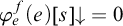





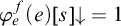





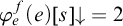


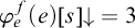


The graph G as described above is easily seen to be planar and having an f-computable plane diagram. Thus, a
$6$
 -coloring c may be obtained by applying
${\mathtt {COL}}^{*}(6)$
-coloring c may be obtained by applying
${\mathtt {COL}}^{*}(6)$
 . Using c, define the following sets for each
$e\in {\mathbb {N}}$
. Using c, define the following sets for each
$e\in {\mathbb {N}}$
 :
:
-
• Let $A_{i}=\{c(v)\mid v\in K_{3}^{j}\text { for some }4i\leq j<4(i+1)\}$
for each
$i<6$
. -
• Let $B_{i}=\{c(v)\mid v\in K_{3}^{j}\text { for some }12i\leq j<12(i+1)\}$
for each
$i<2$
.




We are now ready to define
$g(e)$
 satisfying
${\mathtt {DNR}}(4)$
satisfying
${\mathtt {DNR}}(4)$
 as follows:
-
• If there is some i for which $|A_{i}|=3$
, then define
$g(e)=0$
.Suppose now for a contradiction that
$\varphi _{e}^{f}(e){\downarrow }=g(e)=0$
. By the construction, vertices
$v_{j}$
for each
$4i\leq j<4(i+1)$
must have been enumerated into the
$e^{th}$
component and each
$v_{j}$
is connected to all the vertices in
$K_{3}^{j}$
. Since
$|A_{i}|=3$
and c is a coloring, we have that
$c(v_{j})\notin A_{i}$
for each
$4i\leq j<4(i+1)$
. But the four vertices
$v_{4i},v_{4i+1},v_{4i+2},v_{4i+3}$
are connected as a
$K_{4}$
graph. Then c cannot possibly be a valid
$6$
-coloring. -
• If the previous case does not hold and there is some i such that $|B_{i}|=4$
, then define
$g(e)=1$
.Once again, suppose that
$\varphi _{e}^{f}(e){\downarrow }=g(e)=1$
. Since the previous case does not hold, then it must be that for each
$j<6$
, we have that
$|A_{j}|\geq 4$
. An analysis of the second case of the construction would allow us to conclude that the six new vertices enumerated,
$v_{j}$
for each
$j<6$
is such that
$c(v_{j})\notin A_{j}$
. In particular, since
$A_{j}\subseteq B_{i}$
for each
$3i\leq j<3(i+1)$
, and
$|B_{i}|=4$
, then
$c(v_{j})\notin B_{i}$
for each
$3i\leq j<3(i+1)$
. Then c must fail as a
$6$
-coloring as the vertices
$v_{3i},v_{3i+1},v_{3i+2}$
are connected as a
$K_{3}$
. -
• If neither of the previous cases hold and $B_{0}=B_{1}$
, then define
$g(e)=2$
.Assume that
$\varphi _{e}^{f}(e){\downarrow }=2$
. Then the two new vertices
$v_{0},v_{1}$
enumerated into the
$e^{th}$
component are, respectively, connected to all vertices in
$K_{3}^{j}$
for each
$j<12$
and
$K_{3}^{l}$
for each
$12\leq l<24$
. In particular,
$c(v_{0})\notin B_{0}$
and
$c(v_{1})\notin B_{1}$
. Since the previous cases all do not hold and
$B_{0}=B_{1}$
, then
$|B_{0}|=|B_{1}|\geq 5$
. c cannot possibly be a
$6$
-coloring. -
• If none of the previous cases hold, then define $g(e)=3$
.If none of the previous cases hold, then
$|B_{0}|,|B_{1}|\geq 5$
and
$B_{0}\neq B_{1}$
. This means that
$|B_{0}\cup B_{1}|=6$
. If
$\varphi _{e}^{f}(e){\downarrow }=3$
, then in the
$e^{th}$
component, a vertex
$v_{0}$
must have been enumerated into the
$e^{th}$
component and connected to all other vertices within the component. In particular,
$c(v_{0})\notin B_{0}\cup B_{1}$
, and hence c fails to be a coloring.






















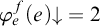














Since the sets
$A_{i}$
 and
$B_{j}$
and
$B_{j}$
 can be computed using c, then g can similarly be obtained from c. Thus,
${\mathtt {DNR}}(4){\leq _{\mathsf {sW}}}{\mathtt {COL}}^{*}(6)$
can be computed using c, then g can similarly be obtained from c. Thus,
${\mathtt {DNR}}(4){\leq _{\mathsf {sW}}}{\mathtt {COL}}^{*}(6)$
 .
.
Unfortunately, it is not clear how the proof above can be easily modified to make the resulting graph connected while retaining an f-computable plane diagram. The main issue lies in using
$K_{4}$
 as a subgraph of the components (which was not required in the proof of Theorem 2.14). In fact, we leave the question of whether
${\mathtt {DNR}}(4){\leq _{\mathsf {W}}}{\mathtt {ConnCOL}}(6)$
as a subgraph of the components (which was not required in the proof of Theorem 2.14). In fact, we leave the question of whether
${\mathtt {DNR}}(4){\leq _{\mathsf {W}}}{\mathtt {ConnCOL}}(6)$
 open. Instead, we prove the following.
Theorem 2.17.
${\mathtt {DNR}}(6){\leq _{\mathsf {sW}}}{\mathtt {ConnCOL}}(6)$
 .
.
Proof. Fix some
$f:{\mathbb {N}}\to {\mathbb {N}}$
 and let
$\left \{\varphi _{e}^{f}(e)\right \}_{e\in {\mathbb {N}}}$
and let
$\left \{\varphi _{e}^{f}(e)\right \}_{e\in {\mathbb {N}}}$
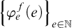 be a standard listing of the f-computable functions. Once again we construct the graph G via components. Each component will consist of 288
$K_{4}$
be a standard listing of the f-computable functions. Once again we construct the graph G via components. Each component will consist of 288
$K_{4}$
 graphs indexed with
$j<288$
graphs indexed with
$j<288$
 . For each
$K_{4}$
. For each
$K_{4}$
 graph, we pick an arbitrary vertex and label it the special vertex.
We proceed with the construction as follows.
-
Stage s: For each $e<s$
not yet declared satisfied, consider the following cases. (Refer to Figure 8 for an illustration. The nodes
$\circ $
represent the newly enumerated vertices whilst
$\blacktriangle $
and
$\bullet $
represent the special and non-special vertices, respectively.)-
• If $\varphi _{e}^{f}(e)[s]{\downarrow }=0$
, then for each
$j<48$
, enumerate vertices
$v_{3j},v_{3j+1},v_{3j+2}$
connected as a
$K_{3}$
graph. In addition, for each
$i<3$
, connect each
$v_{3j+i}$
to the special vertex of
$K_{4}^{6j+2i}$
and the non-special vertices of
$K_{4}^{6j+2i+1}$
.Figure 8The gadget for Theorem 2.17. To reduce clutter, we use $\bullet $
and
$\blacktriangle $
to represent all the non-special and special vertices of the
$K_{4}^{m}$
, respectively.Figure 8. Long description
The diagram consists of four panels arranged in a two by two grid. Each panel begins with a conditional statement followed by a graph structure.
* Top-left panel: Statement reads If phi sub e super f of e equals 0, then for each j less than 48. Below this, three white circular vertices are connected in a line with an arched edge connecting the outer two. Each white vertex is connected to two rectangular blocks below it. There are six blocks labeled K sub 4 super 6j through K sub 4 super 6j plus 5. Each block has a black dot and a black triangle on its top edge.
* Top-right panel: Statement reads If phi sub e super f of e equals 1, then for each j less than 12. The structure features two central white vertices stacked vertically. The top white vertex connects to two upper rectangular blocks labeled K sub 4 super 24j plus 12 through 17 and K sub 4 super 24j plus 18 through 23. The bottom white vertex connects to two lower rectangular blocks labeled K sub 4 super 24j through 5 and K sub 4 super 24j plus 6 through 11. Black dots and triangles mark the connection points.
* Bottom-left panel: Statement reads If phi sub e super f of e equals 2, then for each j less than 6. A single white vertex is positioned between an upper block labeled K sub 4 super 48j plus 24 through 47 and a lower block labeled K sub 4 super 48j through 23. An arrow points from the white vertex to the lower block.
* Bottom-right panel: Statement reads If phi sub e super f of e equals 3, then for each j less than 2. A central white vertex connects to one upper block labeled K sub 4 super 144j plus 96 through 143 and two lower white vertices. These two lower white vertices are connected by a horizontal line and each connects to one of two large lower blocks labeled K sub 4 super 144j through 47 and K sub 4 super 144j plus 48 through 95.
-
• If $\varphi _{e}^{f}(e)[s]{\downarrow }=1$
, then for each
$j<12$
, enumerate vertices
$v_{2j},v_{2j+1}$
and connect
$v_{2j}$
to
$v_{2j+1}$
. We also connect
$v_{2j}$
to all the special vertices of
$K_{4}^{24j+i}$
and all the non-special vertices of
$K_{4}^{24j+i+6}$
for each
$i<6$
. Similarly, connect
$v_{2j+1}$
to all the special vertices of
$K_{4}^{24j+i+12}$
and all the non-special vertices of
$K_{4}^{24j+i+18}$
for each
$i<6$
. -
• If $\varphi _{e}^{f}(e)[s]{\downarrow }=2$
, then for each
$j<6$
, enumerate a vertex
$v_{j}$
and for each
$i<24$
, connect
$v_{j}$
to all the special vertices of
$K_{4}^{48j+i}$
and to all the non-special vertices of
$K_{4}^{48j+i+24}$
. -
• If $\varphi _{e}^{f}(e)[s]{\downarrow }=3$
, then for each
$j<2$
, enumerate
$v_{3j}$
,
$v_{3j+1}$
,
$v_{3j+2}$
connected as a
$K_{3}$
graph. Also connect
$v_{3j+i}$
to the non-special vertices of
$K_{4}^{144j+48i+l}$
for each
$l<48$
. -
• If $\varphi _{e}^{f}(e)[s]{\downarrow }=4$
, then enumerate
$v_{0},v_{1}$
and connect them. Connect
$v_{0}$
to all the non-special vertices of
$K_{4}^{i}$
for each
$i<144$
and connect
$v_{1}$
to all the non-special vertices of
$K_{4}^{j}$
for each
$144\leq j<288$
. -
• If $\varphi _{e}^{f}(e)[s]{\downarrow }=5$
, then enumerate a single vertex
$v_{0}$
and connect it to all the non-special vertices of
$K_{4}^{i}$
for each
$i<288$
.
If one of the above cases holds, then declare e satisfied.
-


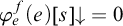




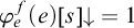


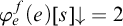


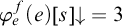


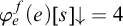



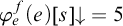


To maintain connectedness of the graph described above, we can arrange the various
$K_{4}$
 graphs in a ‘row’, and for each
$K_{4}$
graphs in a ‘row’, and for each
$K_{4}$
 , enumerate some vertex and connect it to one of the non-special vertices. Then connect these newly enumerated vertices as a path. It is clear that planarity is preserved and the resultant graph is now connected. Hence by
${\mathtt {ConnCOL}}(6)$
, enumerate some vertex and connect it to one of the non-special vertices. Then connect these newly enumerated vertices as a path. It is clear that planarity is preserved and the resultant graph is now connected. Hence by
${\mathtt {ConnCOL}}(6)$
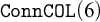 , there is a
$6$
, there is a
$6$
 -coloring c of G. It remains to prove that g satisfying
${\mathtt {DNR}}(6)$
-coloring c of G. It remains to prove that g satisfying
${\mathtt {DNR}}(6)$
 may be computed from c.
Fix some e, and within the
$e^{th}$
 component, for each
$i<288$
component, for each
$i<288$
 , let
, let
-
• $N_{i} =\{c(v)\mid v\in K_{4}^{i}\text { and }v\text { non-special}\}$
; -
• $S_{i} =\{c(v)\mid v\in K_{4}^{i}\text { and }v\text { special}\}$
.


Now consider the following cases:
-
(1) If there exists some $j<6$
such that
$|\bigcup _{48j\leq i<48(j+1)}N_{i}|=3$
, then we consider the following subcases:-
(a) If there exists some i such that $8j\leq i<8(j+1)$
and
$|\bigcup _{l<6}S_{6i+l}|=1$
, then define
$g(e)=0$
. In other words, for each
$l<6,\,N_{6i}=N_{6i+l}$
and
$S_{6i}=S_{6i+l}$
. -
(b) If the previous subcase does not hold and there exists some i such that $2j\leq i<2(j+1)$
and
$|\bigcup _{l<24}S_{24i+l}|=2$
, then define
$g(e)=1$
. Since the previous subcase does not hold, then
$|\bigcup _{l<6}S_{24i+6m+l}|>1$
for each
$m<4$
. In particular, it must be exactly
$2$
. Therefore, we obtain that for each
$m<4$
, $$ \begin{align*}\bigcup_{l<6}S_{24i+l}=\bigcup_{l<6}S_{24i+6m+l}\text{ and }\bigcup_{l<6}N_{24i+l}=\bigcup_{l<6}N_{24i+6m+l}. \end{align*} $$
-
(c) If neither of the previous subcases hold, then define $g(e)=2$
. In particular, it must be the case that for each i such that
$2j\leq i<2(j+1),\,|\bigcup _{l<24}S_{24i+l}|=3$
since c is a
$6$
-coloring. Therefore, $$ \begin{align*}\bigcup_{l<24}S_{48j+l}=\bigcup_{l<24}S_{48j+24+l}\text{ and }\bigcup_{l<24}N_{48j+l}=\bigcup_{l<24}N_{48j+24+l}. \end{align*} $$
Combining the conclusions above with the corresponding actions taken during the construction if $\varphi _{e}^{f}(e)=k\leq 2$
allows us to conclude that c cannot possibly extend to a
$6$
-coloring if
$g(e)=\varphi _{e}^{f}(e)=k\leq 2$
. -
-
(2) Suppose that the previous case does not hold; for every $j<6$
,
$|\bigcup _{48j\leq i<48(j+1)}N_{i}|\geq 4$
. Now consider the following subcases:-
(a) If in addition, there is some $j<2$
for which
$|\bigcup _{144j\leq i<144(j+1)}N_{i}|=4$
, then define
$g(e)=3$
. This implies that for each
$m<3$
, $$ \begin{align*}\bigcup_{l<48}N_{144j+l}=\bigcup_{l<48}N_{144j+48m+l}. \end{align*} $$
-
(b) If the previous subcase does not hold and $|\bigcup _{j<288}N_{j}|=5$
, then define
$g(e)=4$
. Note that we have $$ \begin{align*}\bigcup_{l<144}N_{l}=\bigcup_{l<144}N_{144+l}. \end{align*} $$
-
(c) Otherwise, define $g(e)=5$
. If neither of the previous subcases hold, we must have that
$|\bigcup _{l<288}N_{l}|=6$
.
A simple analysis of the actions taken during the construction if $\varphi _{e}^{f}(e)=k\geq 3$
allows one to conclude that it cannot be that
$g(e)=\varphi _{e}^{f}(e)=k\geq 3$
. -
















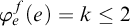












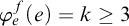

Thus we have that
${\mathtt {DNR}}(6){\leq _{\mathsf {sW}}}{\mathtt {ConnCOL}}(6)$
 .
.
Observe that in the proof above, the graph constructed need not have an f-computable plane diagram. In particular, we cannot f-compute whether or not the special vertex in each
$K_{4}$
 should be embedded as the ‘inner’ or one of the ‘outer’ vertices in a standard drawing of
$K_{4}$
should be embedded as the ‘inner’ or one of the ‘outer’ vertices in a standard drawing of
$K_{4}$
 .
.
When
$n=7$
 , the principles separate even more in the sense that only
${\mathtt {COL}}(7)$
, the principles separate even more in the sense that only
${\mathtt {COL}}(7)$
 is such that there exists some k where
${\mathtt {DNR}}(k){\leq _{\mathsf {W}}}{\mathtt {COL}}(7)$
is such that there exists some k where
${\mathtt {DNR}}(k){\leq _{\mathsf {W}}}{\mathtt {COL}}(7)$
 . For the other principles, we in fact have that
${\mathtt {DNR}}{\not \!\!{\leq _{\mathsf {W}}}}{\mathtt {ConnCOL}}(7),{\mathtt {COL}}^{*}(7)$
. For the other principles, we in fact have that
${\mathtt {DNR}}{\not \!\!{\leq _{\mathsf {W}}}}{\mathtt {ConnCOL}}(7),{\mathtt {COL}}^{*}(7)$
 (see Theorem 3.13).
Theorem 2.18.
${\mathtt {DNR}}(8){\leq _{\mathsf {sW}}}{\mathtt {COL}}(7)$
 .
.
Proof. Fix some
$f:{\mathbb {N}}\to {\mathbb {N}}$
 and let
$\left \{\varphi _{e}^{f}\right \}$
and let
$\left \{\varphi _{e}^{f}\right \}$
 be a standard listing of the f-computable functions. We adopt a similar gadget as before and construct the graph G in diagonalisation components. Each component will contain
$9216\, K_{4}$
be a standard listing of the f-computable functions. We adopt a similar gadget as before and construct the graph G in diagonalisation components. Each component will contain
$9216\, K_{4}$
 graphs (indexed in the superscript).
Now construct G as follows.
-
Stage s: For each $e<s$
not yet declared satisfied, do the following:-
• If $\varphi _{e}^{f}(e)[s]{\downarrow }=0$
, then for each
$j<1152$
, enumerate vertices
$4j+i$
for each
$i<4$
connected as a
$K_{4}$
into the
$e^{th}$
component. For each
$i<4$
, connect each
$v_{4j+i}$
to the special vertex of
$K_{4}^{8j+2i}$
and the non-special vertices of
$K_{4}^{8j+2i+1}$
. -
• If $\varphi _{e}^{f}(e)[s]{\downarrow }=1$
, then for each
$j<192$
, enumerate vertices
$3j+i$
for each
$i<3$
connected as a
$K_{3}$
. For each
$i<3$
and
$l<8$
, connect each
$v_{3j+i}$
to all the special vertices of
$K_{4}^{48j+16i+l}$
and the non-special vertices of
$K_{4}^{48j+16i+8+l}$
. -
• If $\varphi _{e}^{f}(e)[s]{\downarrow }=2$
, then for each
$j<48$
, enumerate vertices
$v_{2j},v_{2j+1}$
and connect
$v_{2j}$
to
$v_{2j+1}$
. For each
$i<2$
and
$l<48$
, connect
$v_{2j+i}$
to all the special vertices of
$K_{4}^{192j+96i+l}$
and all the non-special vertices of
$K_{4}^{192j+96i+48+l}$
. -
• If $\varphi _{e}^{f}(e)[s]{\downarrow }=3$
, then for each
$j<24$
, enumerate a vertex
$v_{j}$
into the
$e^{th}$
component. In addition, for each
$l<192$
, connect
$v_{j}$
to all the special vertices of
$K_{4}^{384j+l}$
and all the non-special vertices of
$K_{4}^{384j+192+l}$
. -
• If $\varphi _{e}^{f}(e)[s]{\downarrow }=4$
, then for each
$j<6$
, enumerate vertices
$v_{4j+i}$
for each
$i<4$
connected as a
$K_{4}$
. In addition, for each
$i<4$
and
$l<384$
, connect
$v_{4j+i}$
to all the non-special vertices of
$K_{4}^{1536j+384i+l}$
. -
• If $\varphi _{e}^{f}(e)[s]{\downarrow }=5$
, then for each
$j<2$
, enumerate vertices
$v_{3j+i}$
for each
$i<3$
connected as a
$K_{3}$
. Also connect for each
$i<3$
and
$l<1536$
,
$v_{3j+i}$
to all the non-special vertices of
$K_{4}^{4608j+1536i+l}$
. -
• If $\varphi _{e}^{f}(e)[s]{\downarrow }=6$
, then enumerate vertices
$v_{0}$
and
$v_{1}$
adjacent to each other. For each
$l<4608$
, connect
$v_{0},v_{1}$
to all the non-special vertices of
$K_{4}^{l}$
and
$K_{4}^{4608+l}$
, respectively. -
• If $\varphi _{e}^{f}(e)[s]{\downarrow }=7$
, then enumerate a single vertex
$v_{0}$
and connect it to all the non-special vertices of
$K_{4}^{l}$
for each
$l<9216$
.
-

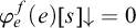


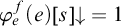


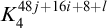
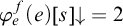


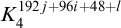
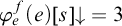


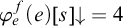


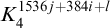
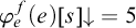


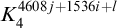
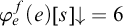


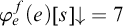


We note here that if we were to make a similar modification to the gadgets above by attempting to connect them as before, the graph will no longer be planar. In fact there should be no easy modification of the gadget which would make the proof work for
${\mathtt {DNR}}(k){\leq _{\mathsf {W}}}{\mathtt {ConnCOL}}(7)$
 for some k (as proved formally in Theorem 3.13). Similarly, this graph G also might not have an f-computable plane diagram since we are unable to f-compute if a special vertex is the ‘inner’ or ‘outer’ vertex in a standard drawing of
$K_{4}$
for some k (as proved formally in Theorem 3.13). Similarly, this graph G also might not have an f-computable plane diagram since we are unable to f-compute if a special vertex is the ‘inner’ or ‘outer’ vertex in a standard drawing of
$K_{4}$
 .
.
It follows from the construction above that the graph is f-computable and planar. Thus,
${\mathtt {COL}}(7)$
 is able to produce a
$7$
is able to produce a
$7$
 -coloring c of the graph. In order to define
$g(e)$
-coloring c of the graph. In order to define
$g(e)$
 , we define the following sets using the behaviour of c in the
$e^{th}$
, we define the following sets using the behaviour of c in the
$e^{th}$
 component:
-
• $N_{i}=\{c(v)\mid v\in K_{4}^{i}\text { and }v\text { non-special}\}$
; -
• $S_{i}=\{c(v)\mid v\in K_{4}^{i}\text { and }v\text { special}\}$
.


Consider the following possibilities:
-
(1) First suppose that there exists $j<24$
such that
$|\bigcup _{384j\leq i<384(j+1)}N_{i}|=3$
. We have the following subcases:-
(a) If there also exists i such that $48j\leq i<48(j+1)$
and
$|\bigcup _{l<8}S_{8i+l}|=1$
, then define
$g(e)=0$
. In this subcase, it is easy to see that for each
$l<8$
, $$ \begin{align*}S_{8i}=S_{8i+l}\text{ and }N_{8i}=N_{8i+l}. \end{align*} $$
-
(b) If the previous subcase does not hold and there exists i such that $8j\leq i<8(j+1)$
and
$|\bigcup _{l<48}S_{48i+l}|=2$
, then define
$g(e)=1$
. Since the previous subcase does not hold, for each
$m<6$
,
$|\bigcup _{l<8}S_{48i+8m+l}|>1$
and thus must be exactly
$2$
. Therefore, for each
$m<6$
, $$ \begin{align*}\bigcup_{l<8}S_{48i+l}=\bigcup_{l<8}S_{48i+8m+l}\text{ and }\bigcup_{l<8}N_{48i+l}=\bigcup_{l<8}N_{48i+8m+l}. \end{align*} $$
-
(c) If both the previous subcases do not hold and there exists i such that $2j\leq i<2(j+1)$
and
$|\bigcup _{l<192}S_{192i+l}|=3$
, then define
$g(e)=2$
. Since Case (1b) does not hold, then for each
$m<4$
,
$|\bigcup _{l<48}S_{192i+48m+l}|>2$
. That is, it must be exactly
$3$
. We thus obtain that for each
$m<4$
, $$ \begin{align*}\bigcup_{l<48}S_{192i+l}=\bigcup_{l<48}S_{192i+48m+l}\text{ and }\bigcup_{l<48}N_{192i+l}=\bigcup_{l<48}N_{192i+48m+l}. \end{align*} $$
-
(d) If none of the previous subcases hold, then define $g(e)=3$
. Since we also have that c is a
$7$
-coloring, then for each i such that
$2j\leq i<2(j+1)$
,
$|\bigcup _{l<192}S_{192i+l}|=4$
. Which is to say that $$ \begin{align*}\bigcup_{l<192}S_{384j+l}=\bigcup_{l<192}S_{384j+192+l}\text{ and }\bigcup_{l<192}N_{384j+l}=\bigcup_{l<192}N_{384j+192+l}. \end{align*} $$
Once again, using the conclusions obtained above and some careful analysis of the cases in the construction, we can conclude that if $g(e)=\varphi _{e}^{f}(e)= k\leq 3$
, c fails to
$7$
-color the
$e^{th}$
component. -
-
(2) Now suppose that for each $j<24$
,
$|\bigcup _{384j\leq i<384(j+1)}N_{i}|\geq 4$
. We consider the following subcases:-
(a) If in addition, there exists $j<6$
such that
$|\bigcup _{l<1536}N_{1536j+l}|=4$
, then define
$g(e)=4$
. With the assumption made in Case (2), we obtain the following. For each
$m<4,$
$$ \begin{align*}\bigcup_{l<384}N_{1536j+l}=\bigcup_{l<384}N_{1536j+384m+l}. \end{align*} $$
-
(b) If there exists $j<2$
such that
$|\bigcup _{l<4608}N_{4608j+l}|=5$
and the previous subcase does not hold, then define
$g(e)=5$
. Using a similar analysis as before, for each
$m<3$
, $$ \begin{align*}\bigcup_{l<1536}N_{4608j+l}=\bigcup_{l<1536}N_{4608j+1536m+l}. \end{align*} $$
-
(c) If $|\bigcup _{l<9216}N_{l}|=6$
and neither of the previous subcases hold, then define
$g(e)=6$
. Since the assumption in Case (2b) fails, then $$ \begin{align*}\bigcup_{l<4608}N_{l}=\bigcup_{4608\leq l<9216}N_{l}. \end{align*} $$
-
(d) Otherwise, define $g(e)=7$
. It is evident that in this subcase,
$|\bigcup _{l<9216}N_{l}|=7$
.
A similar analysis as before can be done to conclude that if $g(e)=\varphi _{e}^{f}(e)=k\geq 4$
, c must fail to be a
$7$
-coloring of the
$e^{th}$
component. -









































Therefore, g as defined satisfies
${\mathtt {DNR}}(8)$
 and is computable from c.
2.4 Reducing
${\mathtt {DNR}}(k,l)$
to coloring principles

As illustrated in Figure 5, when
$n=7,8$
 , the coloring principles seem to weaken considerably as compared to
$n<7$
, the coloring principles seem to weaken considerably as compared to
$n<7$
 . In fact,
${\mathtt {DNR}}{\not \!\!{\leq _{\mathsf {W}}}}{\mathtt {COL}}(8)$
. In fact,
${\mathtt {DNR}}{\not \!\!{\leq _{\mathsf {W}}}}{\mathtt {COL}}(8)$
 (Theorem 3.2). In order to continue the analysis of the level of non-uniformity required, we introduce the following principles (see also [Reference Schmerl and Simpson19, Lemma 2.3]).
Definition 2.19. The following definitions can be made in
${\mathtt {RCA}_{0}}$
 :
:
-
• A trace $\left \{T_{n}\right \}_{n\in {\mathbb {N}}}$
is a sequence of sets. In
${\mathtt {RCA}_{0}}$
, we can interpret such an object as an effective listing of the indexes of the c.e. sets required. -
• Given a function h, a trace is h-bounded if for each $n,\,\left |T_{n}\right |\leq h(n)$
. -
• A trace $\left \{T_{n}\right \}_{n\in {\mathbb {N}}}$
is a c.e. trace if there exists some computable g such that
$T_{n}=W_{g(n)}=\{x\mid \varphi _{g(n)}(x){\downarrow }\}$
for all n. A universal c.e. trace is a c.e. trace where every c.e. set A is equal to
$T_{n}$
for some n. -
• A universal h-bounded c.e. trace is a c.e. trace where for every set c.e. set A, there is some n such that $T_{n}=A\restriction h(n)$
.







As usual, the definition above can be relativised to any oracle f.
Definition 2.20. The following definitions can be made in
${\mathtt {RCA}_{0}}$
 :
:
-
• A function g is approximated by $\tilde {g}$
iff for every
$x,\,\lim _{s\to \infty }\tilde {g}(x,s)=g(x)$
. -
• We say that $\tilde {g}$
is an l-approximation of g if
$\tilde {g}$
approximates g and $$ \begin{align*}\left|\{s\mid \tilde{g}(x,s)\neq\tilde{g}(x,s+1)\}\right|<l+1. \end{align*} $$




Definition 2.21. Let
$\{T_{x}\}_{x\in {\mathbb {N}}}$
 be the universal
$l+1$
be the universal
$l+1$
 -bounded c.e. trace, then
${\mathtt {DNR}}(k,l)$
-bounded c.e. trace, then
${\mathtt {DNR}}(k,l)$
 is the principle:

Evidently, for any
$k\geq 2$
 and
$l\geq 1$
and
$l\geq 1$
 ,
${\mathtt {DNR}}(k,l+1){\leq _{\mathsf {W}}}{\mathtt {DNR}}(k,l){\leq _{\mathsf {W}}}{\mathtt {DNR}}(k)$
,
${\mathtt {DNR}}(k,l+1){\leq _{\mathsf {W}}}{\mathtt {DNR}}(k,l){\leq _{\mathsf {W}}}{\mathtt {DNR}}(k)$
 . Recall that in Section 2.1, in order to diagonalise against the n-colorings when n is large, we use a ‘layered’ gadget. More specifically, we wait for the coloring to first commit on some initial part of the gadget which has been revealed before extending the gadget. Each extension forces the coloring to use up more of its available colors before we finally obtain a diagonalisation. This lends itself nicely into the idea behind using l-approximable functions; roughly speaking, each ‘layer’ in the gadget will correspond to a stage at which the approximation changes. In order to obtain the level of non-unformity required for the reversal of
${\mathtt {COL}}(n)$
. Recall that in Section 2.1, in order to diagonalise against the n-colorings when n is large, we use a ‘layered’ gadget. More specifically, we wait for the coloring to first commit on some initial part of the gadget which has been revealed before extending the gadget. Each extension forces the coloring to use up more of its available colors before we finally obtain a diagonalisation. This lends itself nicely into the idea behind using l-approximable functions; roughly speaking, each ‘layer’ in the gadget will correspond to a stage at which the approximation changes. In order to obtain the level of non-unformity required for the reversal of
${\mathtt {COL}}(n)$
 over
${\mathtt {RCA}_{0}}$
over
${\mathtt {RCA}_{0}}$
 to
${{\mathtt {WKL}}}$
to
${{\mathtt {WKL}}}$
 , we will compare
${\mathtt {DNR}}(k,l)$
, we will compare
${\mathtt {DNR}}(k,l)$
 with the principles
${\mathtt {COL}}(n),{\mathtt {COL}}^{*}(n)$
with the principles
${\mathtt {COL}}(n),{\mathtt {COL}}^{*}(n)$
 , and
${\mathtt {ConnCOL}}(n)$
, and
${\mathtt {ConnCOL}}(n)$
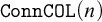 . But we first show that they are each equivalent to
${{\mathtt {WKL}}}$
. But we first show that they are each equivalent to
${{\mathtt {WKL}}}$
 over
${\mathtt {RCA}_{0}}$
over
${\mathtt {RCA}_{0}}$
 .
.
Theorem 2.22.
${\mathtt {RCA}_{0}}\,\vdash\, {\mathtt {DNR}}(k,1)\rightarrow {\mathtt {DNR}}(k)$
 .
.
Proof. Fix some function f and a standard listing of the computable functions
$\left \{\varphi _{e}\right \}_{e\in {\mathbb {N}}}$
 . Let
$\left \{T_{x}^{f}\right \}_{x\in {\mathbb {N}}}$
. Let
$\left \{T_{x}^{f}\right \}_{x\in {\mathbb {N}}}$
 be a universal
$2$
be a universal
$2$
 -bounded c.e. trace. Define p a computable function such that

By
${\mathtt {DNR}}(k,1)$
 , there exists some
$g:{\mathbb {N}}\to \{0,1,\dots ,k-1\}$
, there exists some
$g:{\mathbb {N}}\to \{0,1,\dots ,k-1\}$
 such that for all
$e,x,\,g(p(e,x))\notin T_{p(e,x)}^{f}$
such that for all
$e,x,\,g(p(e,x))\notin T_{p(e,x)}^{f}$
 , and g has a computable
$1$
, and g has a computable
$1$
 -approximation
$\tilde {g}$
-approximation
$\tilde {g}$
 . Define
$g^{*}$
. Define
$g^{*}$
 (non-uniformly) satisfying
${\mathtt {DNR}}(k)$
(non-uniformly) satisfying
${\mathtt {DNR}}(k)$
 as follows:
-
Case 1: If there is some e such that for every x, $\tilde {g}(p(e,x),0)\neq \varphi _{x}^{f}(x)$
, then define
$g^{*}(x)=\tilde {g}(p(e,x),0)$
.
$g^{*}$
clearly exists via
$\Delta _{1}^{0}$
-comprehension and it is evident that
$g^{*}(x){\downarrow }\neq \varphi _{x}^{f}(x)$
for every x. -
Case 2: If for every e, there is some $x_{e}$
such that
$\tilde {g}(p(e,x_{e}),0)=\varphi _{x_{e}}^{f}(x_{e})$
, then define
$g^{*}(e)=\tilde {g}(p(e,x_{e}),s_{e})$
where
$s_{e}$
is the first stage at which
$\tilde {g}(p(e,x_{e}),s_{e})\neq \tilde {g}(p(e,x_{e}),0)$
.Since
$\tilde {g}$
is a
$1$
-approximation to g (satisfying
${\mathtt {DNR}}(k,1)$
), then there must be some stage at which
$\tilde {g}(p(e,x_{e}),s)\neq \tilde {g}(p(e,x_{e}),0)$
. Otherwise
$\tilde {g}(p(e,x_{e}),s)=\tilde {g}(p(e,x_{e}),0)=\varphi _{x_{e}}^{f}(x_{e}){\downarrow }$
at every stage s which contradicts the assumption that
$g(p(e,x_{e}))\notin T_{p(e,x_{e})}^{f}$
. Since s must exist, then there is always a least one and thus
$g^{*}$
exists by
$\Delta _{1}^{0}$
-comprehension.Suppose now for a contradiction that
$\varphi _{e}^{f}(e){\downarrow }=g^{*}(e)=\tilde {g}(p(e,x_{e}),s_{e})$
. Since
$\tilde {g}$
is a
$1$
-approximation to g, that means that
$g(p(e,x_{e}))=\tilde {g}(p(e,x_{e}),s_{e})$
. Then we have that
$g(p(e,x_{e}))=\varphi _{e}^{f}(e){\downarrow }$
a contradiction. Thus
$g^{*}$
satisfies
${\mathtt {DNR}}(k)$
.
























In any case, we have that
$g^{*}$
 exists and satisfies
${\mathtt {DNR}}(k)$
exists and satisfies
${\mathtt {DNR}}(k)$
 .
.
Theorem 2.23. For any
$l>1$
 ,
${\mathtt {RCA}_{0}}\,\vdash\, {\mathtt {DNR}}(k,l+1)\rightarrow {\mathtt {DNR}}(k)\vee {\mathtt {DNR}}(k,l)$
,
${\mathtt {RCA}_{0}}\,\vdash\, {\mathtt {DNR}}(k,l+1)\rightarrow {\mathtt {DNR}}(k)\vee {\mathtt {DNR}}(k,l)$
 .
.
Proof. Fix some function f and the standard listing of the computable functions
$\{\varphi _{e}\}_{e\in {\mathbb {N}}}$
 . Let
$\left \{T_{x}^{f}\right \}_{x\in {\mathbb {N}}}$
. Let
$\left \{T_{x}^{f}\right \}_{x\in {\mathbb {N}}}$
 and
$\{U_{x}^{f}\}_{x\in {\mathbb {N}}}$
and
$\{U_{x}^{f}\}_{x\in {\mathbb {N}}}$
 be an
$l+1$
be an
$l+1$
 -bounded and
$l+2$
-bounded and
$l+2$
 -bounded universal c.e. trace, respectively. Define p a computable functions such that

By
${\mathtt {DNR}}(k,l+1)$
 , there must exist g such that for all
$e,x,\,g(p(e,x))\notin U_{p(e,x)}^{f}$
, there must exist g such that for all
$e,x,\,g(p(e,x))\notin U_{p(e,x)}^{f}$
 with a computable
$l+1$
with a computable
$l+1$
 -approximation
$\tilde {g}$
-approximation
$\tilde {g}$
 . We proceed non-uniformly and aim to define a function h which satisfies
${\mathtt {DNR}}(k)\vee {\mathtt {DNR}}(k,l)$
. We proceed non-uniformly and aim to define a function h which satisfies
${\mathtt {DNR}}(k)\vee {\mathtt {DNR}}(k,l)$
 .
.
-
Case 1: If there is some e such that for every x, $\tilde {g}(p(e,x),0)\neq \varphi _{x}^{f}(x)$
, then define
$h(x)=\tilde {g}(p(e,x),0)$
. h clearly exists via
$\Delta _{1}^{0}$
-comprehension and satisfies
${\mathtt {DNR}}(k)$
. -
Case 2: If for every e, there is some $x_{e}$
such that
$\tilde {g}(p(e,x_{e}),0)=\varphi _{x_{e}}^{f}(x_{e})$
, then define
$h(e)=\lim _{s\to \infty }\tilde {g}(p(e,x_{e}),s+s_{e})$
where
$s_{e}$
is the first stage at which
$\tilde {g}(p(e,x_{e}),s_{e})\neq \tilde {g}(p(e,x_{e}),0)$
. By assumption that g satisfies
${\mathtt {DNR}}(k,l+1)$
, then
$g(p(e,x_{e}))\notin U_{p(e,x_{e})}^{f}$
. That is,
$h(e)=g(p(e,x_{e}))\notin T_{e}^{f}$
. It remains thus to show that there is some computable
$\tilde {h}$
which is an l-approximation of h.For similar reasons as before,
$s_{e}$
exists and thus by defining
$\tilde {h}(e,s)=\tilde {g}(p(e,x_{e}),s+s_{e})$
,
$\tilde {h}$
exists via
$\Delta _{1}^{0}$
-comprehension. Since we have that
$\tilde {g}$
is an
$l+1$
-approximation and
$\tilde {g}(p(e,x_{e}),s_{e}-1)\neq \tilde {g}(p(e,x_{e}),s_{e})$
, then it is clear that
$\tilde {h}$
is an l-approximation.















Thus we have that the h defined satisfies either
${\mathtt {DNR}}(k)$
 or
${\mathtt {DNR}}(k,l)$
or
${\mathtt {DNR}}(k,l)$
 .
.
Corollary 2.24. For any
$k,l$
 ,
${\mathtt {RCA}_{0}}\,\vdash\, {\mathtt {DNR}}(k,l)\rightarrow {\mathtt {DNR}}(k).$
,
${\mathtt {RCA}_{0}}\,\vdash\, {\mathtt {DNR}}(k,l)\rightarrow {\mathtt {DNR}}(k).$

We are now ready to prove the main result of this section.
Theorem 2.25. For each
$n\geq 4$
 , there exists
$k_{n},l_{n}$
, there exists
$k_{n},l_{n}$
 such that

Proof. First, given n, we pick
$k_{n},l_{n}$
 as follows:
-
• $l_{n}=\left \lfloor \frac {n}{2}\right \rfloor -1$
. -
• $q_{n,l_{n}+1}=2$
, the number of vertices in the
$l_{n}+1$
-th layer of a component (both properly defined in the construction). -
• Proceed recursively for each $i<l_{n}+1$
and define
$q_{n,i-1}$
as follows. Let
$p_{l_{n}+1}=2$
, and let
$p_{i-1}=\sum _{j=i}^{l_{n}+1}2p_{j}$
. Then define
$q_{n,i-1}=(p_{i-1}-1)C(n,2)+1$
, where
$C(x,y)$
is the binomial coefficient. Observe that by pigeonhole principle,
$q_{n,i-1}$
is the number of pairs of vertices that when colored with some valid n-coloring, at least
$p_{i-1}$
many pairs of vertices have the same two colors. -
• Define $k_{n}=\max \left \{\langle i,p_{i}^{*}\rangle \mid i<l_{n}+1\right \}+1$
, where
$p_{i}^{*}$
is an encoding of a possible
$p_{i}$
-tuple of pairs of vertices in the
$i^{th}$
layer (to be defined later).
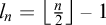


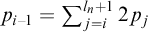



Fix some function
$f:{\mathbb {N}}\to {\mathbb {N}}$
 and the
$l_{n}+1$
and the
$l_{n}+1$
 -bounded universal trace
$\{T_{e}^{f}\}$
-bounded universal trace
$\{T_{e}^{f}\}$
 . We now construct an (f-computable) connected planar graph G with an f-computable plane diagram. The rough idea is that in order to obtain the
${\mathtt {DNR}}(k_{n},l_{n})$
. We now construct an (f-computable) connected planar graph G with an f-computable plane diagram. The rough idea is that in order to obtain the
${\mathtt {DNR}}(k_{n},l_{n})$
 function, we build the gadget in layers. Each time some new element is enumerated into the universal trace, we extend (in the sense of Definition 2.5) the gadget to the next layer, ensuring that any valid coloring encodes information regarding the element which just entered the universal trace. We now construct the graph in (diagonalisation) components as before.
-
Stage s: Begin the $s^{th}$
component by enumerating
$2q_{n,0}$
many vertices and connecting them as a path. These vertices shall be referred to as the
$0^{th}$
layer of the
$s^{th}$
component.For each
$e<s$
, let i be the greatest such that the
$i^{th}$
layer has been defined in the
$e^{th}$
component and do the following.For each
$t\in T_{e}^{f}[s]$
, check if
$t=\langle i,p_{i}^{*}\rangle $
for some
$p_{i}^{*}$
, an encoding of a
$p_{i}$
-tuple consisting of entries
$<q_{n,i}$
. If there are no
$t\in T_{e}^{f}[s]$
which satisfy the desired condition, then do nothing and attend to the next
$e<s$
or proceed to the next stage if there are no more
$e<s$
to attend to.If there is some
$t_{i}\in T_{e}^{f}[s]$
such that
$t_{i}=\langle i,p_{i}^{*}\rangle $
for some
$p_{i}^{*}$
, then enumerate new vertices
$v_{j}$
for each
$j<2q_{n,i+1}$
into the
$e^{th}$
component. We refer to these vertices as the
$i+1$
-th layer of the
$e^{th}$
component. For each
$j<2q_{n,i+1}$
, and for each
$r<i+1$
, connect
$v_{j}$
to some pair of vertices encoded by
$p_{r}^{*}$
in the
$r^{th}$
layer, where
$\langle r,p_{r}^{*}\rangle \in T_{e}^{f}[s]$
(see Figure 9 for an illustrationFootnote
5
). Finally, within the
$i+1$
-th layer, connect
$v_{2j}$
to
$v_{2j+1}$
for each
$j<q_{n,i+1}$
. Note that this procedure is well-defined as the
$i+1$
-th layer can only exist at the
$s^{th}$
stage if for each
$r\leq i$
, some element in
$T_{e}^{f}[s]$
is of the form
$\langle r,p_{r}^{*}\rangle $
. By some careful arrangement of the connections as illustrated in Figure 9, each component can be made planar.Once we are done acting for each
$e<s$
, proceed to stage
$s+1$
.Figure 9Reversal of ${\mathtt {COL}}(n)$
. The dashed lines represent some number of vertices and edges; the
$0^{th}$
layer is a path.


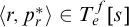


It is easy to see that the graph can be made connected with an f-computable plane diagram. By the choice of
$q_{n,i}$
 , there is always ‘sufficient space’ to connect each new layer to the previous ones.
Applying
${\mathtt {ConnCOL}}(n)$
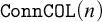 , there is an n-coloring c of the graph G as described in the construction (we could also use
${\mathtt {COL}}(n)$
, there is an n-coloring c of the graph G as described in the construction (we could also use
${\mathtt {COL}}(n)$
 or
${\mathtt {COL}}^{*}(n)$
or
${\mathtt {COL}}^{*}(n)$
 in place of
${\mathtt {ConnCOL}}(n)$
in place of
${\mathtt {ConnCOL}}(n)$
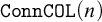 ). Now we attempt to define an
$l_{n}$
). Now we attempt to define an
$l_{n}$
 -approximation
$\tilde {g}$
-approximation
$\tilde {g}$
 satisfying
${\mathtt {DNR}}(k_{n},l_{n})$
satisfying
${\mathtt {DNR}}(k_{n},l_{n})$
 .
.
To define an
$l_{n}$
 -approximation, the intuitive idea is that each layer aims to ‘block’ off two colors and corresponds roughly to each change in the approximation. In the case that all the colors are used up, we then show that the final value must avoid the trace. We provide the details as follows.
Fix some
$e\in {\mathbb {N}}$
 and consider the coloring c within the
$e^{th}$
and consider the coloring c within the
$e^{th}$
 component. Define
$\tilde {g}(e,0)=\langle 0,p_{0}^{*}\rangle $
component. Define
$\tilde {g}(e,0)=\langle 0,p_{0}^{*}\rangle $
 , where
$p_{0}^{*}$
, where
$p_{0}^{*}$
 is the encoding of the first
$q_{n,0}$
is the encoding of the first
$q_{n,0}$
 many pairs in the
$0^{th}$
many pairs in the
$0^{th}$
 layer of the
$e^{th}$
layer of the
$e^{th}$
 component that is colored the same two colors by c. Without loss of generality, we may assume that these two colors are
$0$
component that is colored the same two colors by c. Without loss of generality, we may assume that these two colors are
$0$
 and
$1$
and
$1$
 . Now suppose inductively that
$\tilde {g}(e,s)$
. Now suppose inductively that
$\tilde {g}(e,s)$
 is some pair
$\langle i,p_{i}^{*}\rangle $
is some pair
$\langle i,p_{i}^{*}\rangle $
 where
$p_{i}^{*}$
where
$p_{i}^{*}$
 is an encoding of a
$p_{i}$
is an encoding of a
$p_{i}$
 -tuple with entries
$<q_{n,i}$
-tuple with entries
$<q_{n,i}$
 . Furthermore, this
$p_{i}$
. Furthermore, this
$p_{i}$
 -tuple encoded by
$\tilde {g}(e,s)$
-tuple encoded by
$\tilde {g}(e,s)$
 is colored
$2i,2i+1$
is colored
$2i,2i+1$
 by c and the
$i^{th}$
by c and the
$i^{th}$
 layer exists in the
$e^{th}$
layer exists in the
$e^{th}$
 gadget. We now aim to define
$\tilde {g}(e,s+1)$
gadget. We now aim to define
$\tilde {g}(e,s+1)$
 .
.
If
$\tilde {g}(e,s)\notin T_{e}^{f}[s+1]$
 , then let
$\tilde {g}(e,s+1)=\tilde {g}(e,s)$
, then let
$\tilde {g}(e,s+1)=\tilde {g}(e,s)$
 . In particular, observe that the desired property is satisfied. If we instead have that
$\tilde {g}(e,s)\in T_{e}^{f}[s+1]$
. In particular, observe that the desired property is satisfied. If we instead have that
$\tilde {g}(e,s)\in T_{e}^{f}[s+1]$
 , then some element t must have entered
$T_{e}^{f}$
, then some element t must have entered
$T_{e}^{f}$
 at stage
$s+1$
at stage
$s+1$
 and must be equal to
$\langle i,p_{i}^{*}\rangle $
and must be equal to
$\langle i,p_{i}^{*}\rangle $
 (the value of
$\tilde {g}(e,s)$
(the value of
$\tilde {g}(e,s)$
 ). When this happens in the construction, the
$i+1$
). When this happens in the construction, the
$i+1$
 -th layer consisting of
$q_{n,i+1}$
-th layer consisting of
$q_{n,i+1}$
 many pairs of vertices must have been enumerated into the
$e^{th}$
many pairs of vertices must have been enumerated into the
$e^{th}$
 component. Furthermore, each vertex in the
$i+1$
component. Furthermore, each vertex in the
$i+1$
 -th layer is connected to some pair of vertices in each layer
$\leq i$
-th layer is connected to some pair of vertices in each layer
$\leq i$
 , which is encoded by some
$t_{r}=\langle r,p_{r}^{*}\rangle \in T_{e}^{f}[s+1]$
, which is encoded by some
$t_{r}=\langle r,p_{r}^{*}\rangle \in T_{e}^{f}[s+1]$
 for each
$r\leq i$
for each
$r\leq i$
 as described in the construction. By the inductive hypothesis, this means that each vertex in the
$i+1$
as described in the construction. By the inductive hypothesis, this means that each vertex in the
$i+1$
 -th layer is adjacent to vertices colored
$0,1,\dots ,2i,2i+1$
-th layer is adjacent to vertices colored
$0,1,\dots ,2i,2i+1$
 . In order for c to be a valid coloring, none of the vertices in the
$i+1$
. In order for c to be a valid coloring, none of the vertices in the
$i+1$
 -th layer can be colored with the first
$2i+2$
-th layer can be colored with the first
$2i+2$
 colors. In addition, the vertices in the
$i+1$
colors. In addition, the vertices in the
$i+1$
 -th layer are also connected as pairs, and by pigeonhole principle, there are at least
$p_{i+1}$
-th layer are also connected as pairs, and by pigeonhole principle, there are at least
$p_{i+1}$
 many pairs colored the same two colors. Without loss of generality, we may assume that these colors are
$2i+2,2i+3$
many pairs colored the same two colors. Without loss of generality, we may assume that these colors are
$2i+2,2i+3$
 as desired. Observe also that
$\tilde {g}$
as desired. Observe also that
$\tilde {g}$
 is computable from
$f\oplus c$
is computable from
$f\oplus c$
 .
.
Since we are defining
$\tilde {g}$
 , in order to make it an
$l_{n}$
, in order to make it an
$l_{n}$
 -approximation, we simply stop changing its value once it has used up all
$l_{n}$
-approximation, we simply stop changing its value once it has used up all
$l_{n}$
 many changes. Now suppose for a contradiction that
$\lim _{s\to \infty }\tilde {g}(e,s)\in T_{e}^{f}$
many changes. Now suppose for a contradiction that
$\lim _{s\to \infty }\tilde {g}(e,s)\in T_{e}^{f}$
 . Let
$s_{0}=0$
. Let
$s_{0}=0$
 and
$s_{i}$
and
$s_{i}$
 be the least stage such that
$\tilde {g}(e,s_{i-1})\neq \tilde {g}(e,s_{i})$
be the least stage such that
$\tilde {g}(e,s_{i-1})\neq \tilde {g}(e,s_{i})$
 . Since
$\tilde {g}$
. Since
$\tilde {g}$
 is an
$l_{n}$
is an
$l_{n}$
 -approximation, we obtain that

By choice of
$s_{i}$
 , we also have that
$\tilde {g}(e,s_{i})=\langle i,p_{i}^{*}\rangle $
, we also have that
$\tilde {g}(e,s_{i})=\langle i,p_{i}^{*}\rangle $
 for each i. This implies that

because
$\tilde {g}(e,s)\neq \tilde {g}(e,s-1)$
 only if
$\tilde {g}(e,s-1)\in T_{e}^{f}[s]$
only if
$\tilde {g}(e,s-1)\in T_{e}^{f}[s]$
 . We also have that
$\tilde {g}(e,s_{i})=\langle i,p_{i}^{*}\rangle $
. We also have that
$\tilde {g}(e,s_{i})=\langle i,p_{i}^{*}\rangle $
 encodes
$p_{i}$
encodes
$p_{i}$
 many pairs of vertices in the
$i^{th}$
many pairs of vertices in the
$i^{th}$
 layer colored with
$2i,2i+1$
layer colored with
$2i,2i+1$
 . Consider the
$l_{n}+1$
. Consider the
$l_{n}+1$
 -th layer (consisting of a pair of vertices) in the
$e^{th}$
-th layer (consisting of a pair of vertices) in the
$e^{th}$
 component. Each vertex in this layer is connected to a pair of vertices from each previous layer; in order for c to be a valid coloring, the vertices in the
$l_{n}+1$
component. Each vertex in this layer is connected to a pair of vertices from each previous layer; in order for c to be a valid coloring, the vertices in the
$l_{n}+1$
 -th layer cannot be colored with colors
$0,1,\dots ,2l_{n}+1$
-th layer cannot be colored with colors
$0,1,\dots ,2l_{n}+1$
 . However, by choice of
$l_{n}$
. However, by choice of
$l_{n}$
 , we obtain that
$2l_{n}+1\geq n-2$
, we obtain that
$2l_{n}+1\geq n-2$
 . Then c has only one remaining color left to color the two adjacent vertices in the
$l_{n}+1$
. Then c has only one remaining color left to color the two adjacent vertices in the
$l_{n}+1$
 -th layer. Thus, it must be that
$\lim _{s\to \infty }\tilde {g}(e,s)\notin T_{e}^{f}$
-th layer. Thus, it must be that
$\lim _{s\to \infty }\tilde {g}(e,s)\notin T_{e}^{f}$
 . Furthermore, by choice of
$k_{n}$
. Furthermore, by choice of
$k_{n}$
 , it is also evident that for each s,
$\tilde {g}(e,s)<k_{n}$
, it is also evident that for each s,
$\tilde {g}(e,s)<k_{n}$
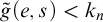 . Therefore,
$\tilde {g}$
. Therefore,
$\tilde {g}$
 satisfies
${\mathtt {DNR}}(k_{n},l_{n})$
satisfies
${\mathtt {DNR}}(k_{n},l_{n})$
 .
.
As before, it is not hard to see that the proof above can be carried out in
${\mathtt {RCA}_{0}}$
 . However, in this more general approach, we note that the proof is rather inefficient with the parameters. In particular, for the cases of
$n=5,6,7$
. However, in this more general approach, we note that the proof is rather inefficient with the parameters. In particular, for the cases of
$n=5,6,7$
 , one can easily compute that we reverse the principles
${\mathtt {COL}}(n),\,{\mathtt {ConnCOL}}(n)$
, one can easily compute that we reverse the principles
${\mathtt {COL}}(n),\,{\mathtt {ConnCOL}}(n)$
 , and
${\mathtt {COL}}^{*}(n)$
, and
${\mathtt {COL}}^{*}(n)$
 to some
${\mathtt {DNR}}(k_{n},l_{n})$
to some
${\mathtt {DNR}}(k_{n},l_{n})$
 for
$l_{n}\geq 1$
for
$l_{n}\geq 1$
 , and a rather large
$k_{n}$
, and a rather large
$k_{n}$
 . Additionally, the reversals of the various
${\mathtt {DNR}}(k_{n},l_{n})$
. Additionally, the reversals of the various
${\mathtt {DNR}}(k_{n},l_{n})$
 principles to
${{\mathtt {WKL}}}$
principles to
${{\mathtt {WKL}}}$
 over
${\mathtt {RCA}_{0}}$
over
${\mathtt {RCA}_{0}}$
 as presented in Theorems 2.22 and 2.23 are also non-uniform (which we suspect is also necessary). In this sense, the proofs presented in Section 2.3 are ‘closer’ to uniform reversals to
${{\mathtt {WKL}}}$
as presented in Theorems 2.22 and 2.23 are also non-uniform (which we suspect is also necessary). In this sense, the proofs presented in Section 2.3 are ‘closer’ to uniform reversals to
${{\mathtt {WKL}}}$
 than the proof presented above. Nonetheless, it provides general bounds for the level of non-uniformity required in the reversals.
3 Non-reductions between the principles
In Section 2, we’ve obtained several positive results reducing variants of
${\mathtt {DNR}}$
 principles to various coloring principles. In this section, we focus on the non-reductions, showing that non-uniformity in certain reversals is necessary.
3.1 Basic coloring principles
We first analyse the uniformity of reductions between the
${\mathtt {DNR}}$
 principles and
${\mathtt {COL}}$
principles and
${\mathtt {COL}}$
 principles. Recall (Definition 2.5) that we use
$G\subseteq G'$
principles. Recall (Definition 2.5) that we use
$G\subseteq G'$
 to denote that G is an induced subgraph of
$G'$
to denote that G is an induced subgraph of
$G'$
 , equivalently, we say that
$G'$
, equivalently, we say that
$G'$
 is an extension of G. We shall continue to use this notation for the rest of this section. To compare the Weihrauch degrees of the coloring principles, we require the following lemma.
Lemma 3.1. Let H be a finite planar graph. If h is a k-coloring of H, then for any countable planar graph
$H'\supseteq H$
 , there is some
$k+4$
, there is some
$k+4$
 -coloring
$h'$
-coloring
$h'$
 of
$H'$
of
$H'$
 such that
$h'\supseteq h$
such that
$h'\supseteq h$
 .
.
Proof. Let H be a finite planar graph with a k-coloring h. Suppose that
$H'$
 is some countable planar graph with H as a subgraph. Since
$H'$
is some countable planar graph with H as a subgraph. Since
$H'$
 is planar, then so is
$H'\setminus H$
is planar, then so is
$H'\setminus H$
 and it must thus have a
$4$
and it must thus have a
$4$
 -coloring c. We then define a
$k+4$
-coloring c. We then define a
$k+4$
 -coloring
$h'$
-coloring
$h'$
 of
$H'$
of
$H'$
 as follows.

It is clear that
$h'\supseteq h$
 is a valid
$k+4$
is a valid
$k+4$
 -coloring of
$H'$
-coloring of
$H'$
 .
.
Theorem 3.2.
${\mathtt {DNR}}{\not \!\!{\leq _{\mathsf {W}}}} {\mathtt {COL}}(8)$
 .
.
Proof. Suppose to the contrary that
${\mathtt {DNR}}{\leq _{\mathsf {W}}} {\mathtt {COL}}(8)$
 . Let
$f=0^{\omega }$
. Let
$f=0^{\omega }$
 and for each s, let
$f_{s}=0^{s}$
and for each s, let
$f_{s}=0^{s}$
 . Then there exists some
$\Phi $
. Then there exists some
$\Phi $
 such that
$\Phi (f)$
such that
$\Phi (f)$
 produces (the code) of some countable computable planar graph G. Furthermore, there is some
$\Psi $
produces (the code) of some countable computable planar graph G. Furthermore, there is some
$\Psi $
 such that for any
$8$
such that for any
$8$
 -coloring h of G,
$\Psi (h\oplus f)$
-coloring h of G,
$\Psi (h\oplus f)$
 satisfies
${\mathtt {DNR}}$
satisfies
${\mathtt {DNR}}$
 .
.
Define
$\psi ^{f}(x)$
 as follows. Search for an s and
$\sigma $
as follows. Search for an s and
$\sigma $
 such that
$\sigma $
such that
$\sigma $
 is a
$4$
is a
$4$
 -coloring of
$\Phi (f_{s})\subseteq G$
-coloring of
$\Phi (f_{s})\subseteq G$
 and
$\Psi (\sigma \oplus f_{s})(x)[s]{\downarrow }$
and
$\Psi (\sigma \oplus f_{s})(x)[s]{\downarrow }$
 . Then
$\psi ^{f}(x)$
. Then
$\psi ^{f}(x)$
 outputs the value of the computation. Since
$G_{s}=\Phi (f_{s})$
outputs the value of the computation. Since
$G_{s}=\Phi (f_{s})$
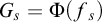 is computable in f, and also a finite graph, then for each s, we can search through all possible
$4$
is computable in f, and also a finite graph, then for each s, we can search through all possible
$4$
 -colorings,
$\sigma $
-colorings,
$\sigma $
 , of
$G_{s}$
, of
$G_{s}$
 and check if
$\Psi (\sigma \oplus f_{s})(x)[s]{\downarrow }$
and check if
$\Psi (\sigma \oplus f_{s})(x)[s]{\downarrow }$
 . By the recursion theorem, we may assume that the index of
$\psi $
. By the recursion theorem, we may assume that the index of
$\psi $
 is x, i.e.,
$\psi ^{f}=\varphi _{x}^{f}$
is x, i.e.,
$\psi ^{f}=\varphi _{x}^{f}$
 . We claim that
$\psi ^{f}(x){\downarrow }$
. We claim that
$\psi ^{f}(x){\downarrow }$
 . Since
$G=\Phi (f)$
. Since
$G=\Phi (f)$
 is planar, there should exist some
$4$
is planar, there should exist some
$4$
 -coloring g of
$\Phi (f)$
-coloring g of
$\Phi (f)$
 . Then, there must be some s such that
$\Psi (g\restriction s\oplus f_{s})(x)[s]{\downarrow }$
. Then, there must be some s such that
$\Psi (g\restriction s\oplus f_{s})(x)[s]{\downarrow }$
 as
$\Psi (g\oplus f)$
as
$\Psi (g\oplus f)$
 is assumed to be total provided g is an
$8$
is assumed to be total provided g is an
$8$
 -coloring of
$\Phi (f)$
-coloring of
$\Phi (f)$
 . Thus,
$\psi ^{f}(x)$
. Thus,
$\psi ^{f}(x)$
 will converge by the time it finds
$g\restriction s$
will converge by the time it finds
$g\restriction s$
 .
.
Evidently, the
$\sigma $
 found by
$\psi ^{f}(x)$
found by
$\psi ^{f}(x)$
 might not extend to a
$4$
might not extend to a
$4$
 -coloring of G; in particular
$\sigma $
-coloring of G; in particular
$\sigma $
 need not be
$g\restriction s$
need not be
$g\restriction s$
 . In order to preserve the computation
$\Psi (\sigma \oplus f_{s})(x)$
. In order to preserve the computation
$\Psi (\sigma \oplus f_{s})(x)$
 , we use Lemma 3.1 to extend
$\sigma $
, we use Lemma 3.1 to extend
$\sigma $
 to an
$8$
to an
$8$
 -coloring, h, of G. As a result, we obtain that

A contradiction to the assumption that
$\Psi (h\oplus f)$
 satisfies
${\mathtt {DNR}}$
satisfies
${\mathtt {DNR}}$
 for any
$8$
for any
$8$
 -coloring h of
$\Phi (f)$
-coloring h of
$\Phi (f)$
 .
.
Theorem 3.3. For any
$n>0$
 and for any
$i<4$
and for any
$i<4$
 ,
${\mathtt {COL}}(4n+i){\not \!\!{\leq _{\mathsf {W}}}}{\mathtt {COL}}(4(n+1))$
,
${\mathtt {COL}}(4n+i){\not \!\!{\leq _{\mathsf {W}}}}{\mathtt {COL}}(4(n+1))$
 .
.
This theorem is a natural extension of Theorem 3.2 (take
$i=0$
 and
$n=1$
and
$n=1$
 ). We extend the ideas used in the proof earlier as follows. Define a graph G using the same gadgets as in Theorem 2.7, and color some initial part of
$H=\Phi (G)$
). We extend the ideas used in the proof earlier as follows. Define a graph G using the same gadgets as in Theorem 2.7, and color some initial part of
$H=\Phi (G)$
 with some
$4$
with some
$4$
 -coloring h. Once
$g=\Psi (h\oplus G)$
-coloring h. Once
$g=\Psi (h\oplus G)$
 has converged on the initial part of the gadget, then we extend the gadget in the same way as before, ensuring that g now has four less colors available to it to color the rest of the gadget. In order to preserve this initial part of g, we then extend h to an
$8$
has converged on the initial part of the gadget, then we extend the gadget in the same way as before, ensuring that g now has four less colors available to it to color the rest of the gadget. In order to preserve this initial part of g, we then extend h to an
$8$
 coloring using Lemma 3.1. As long as we are always able to extend h ‘more than’ g, then g must fail as a coloring.
Proof of Theorem 3.3
Suppose to the contrary that
${\mathtt {COL}}(4n+i){\leq _{\mathsf {W}}}{\mathtt {COL}}(4(n+1))$
 for some
$i<4$
for some
$i<4$
 . We aim to construct a graph G such that for some
$4(n+1)$
. We aim to construct a graph G such that for some
$4(n+1)$
 -coloring h of
$H=\Phi (G)$
-coloring h of
$H=\Phi (G)$
 ,
$g=\Psi (h\oplus G)$
,
$g=\Psi (h\oplus G)$
 fails to be a
$4n+i$
fails to be a
$4n+i$
 -coloring of G. We will follow the proof of Theorem 2.7 closely. Begin by enumerating sufficiently many
$K_{4}$
-coloring of G. We will follow the proof of Theorem 2.7 closely. Begin by enumerating sufficiently many
$K_{4}$
 graphs to construct a
$W_{m}$
graphs to construct a
$W_{m}$
 (as described in Section 2.1) where m is the least such that
$m\geq \lceil (4n+i)/4\rceil $
(as described in Section 2.1) where m is the least such that
$m\geq \lceil (4n+i)/4\rceil $
 , and let this graph be denoted by
$G_{0}$
, and let this graph be denoted by
$G_{0}$
 .
.
During the construction, we will attempt to define some appropriate coloring
$\sigma $
 of
$H_{s}=\Phi (G_{s})$
of
$H_{s}=\Phi (G_{s})$
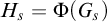 while waiting for
$\Psi (\sigma \oplus G_{s})$
while waiting for
$\Psi (\sigma \oplus G_{s})$
 to converge on the vertices of
$W_{m}$
to converge on the vertices of
$W_{m}$
 enumerated thus far in
$G_{s}$
enumerated thus far in
$G_{s}$
 . For stages during which we are waiting, let
$G_{s+1}$
. For stages during which we are waiting, let
$G_{s+1}$
 be the union of the graph
$G_{s}$
be the union of the graph
$G_{s}$
 with a single isolated vertex. It is clear that if we wait forever,
$\bigcup _{s}G_{s}$
with a single isolated vertex. It is clear that if we wait forever,
$\bigcup _{s}G_{s}$
 is a countable planar graph and thus so is
$H=\Phi \left (\bigcup _{s}G_{s}\right )$
is a countable planar graph and thus so is
$H=\Phi \left (\bigcup _{s}G_{s}\right )$
 . Fix some
$4$
. Fix some
$4$
 -coloring
$h_{0}$
-coloring
$h_{0}$
 of H. By the assumption that
${\mathtt {COL}}(4n+i){\leq _{\mathsf {W}}} {\mathtt {COL}}(4(n+1))$
of H. By the assumption that
${\mathtt {COL}}(4n+i){\leq _{\mathsf {W}}} {\mathtt {COL}}(4(n+1))$
 is witnessed by
$\Phi ,\Psi $
is witnessed by
$\Phi ,\Psi $
 ,
$g=\Psi (h_{0}\oplus G)$
,
$g=\Psi (h_{0}\oplus G)$
 must be some
$4n+i$
must be some
$4n+i$
 coloring of G. In particular, since we are only waiting for g to converge on the finitely many vertices of
$W_{m}$
coloring of G. In particular, since we are only waiting for g to converge on the finitely many vertices of
$W_{m}$
 enumerated thus far, there must be some finite stage at which it happens. Let this stage be
$s_{0}$
enumerated thus far, there must be some finite stage at which it happens. Let this stage be
$s_{0}$
 and let
$G_{s_{0}+1}$
and let
$G_{s_{0}+1}$
 be the graph where the appropriate
$K_{4}$
be the graph where the appropriate
$K_{4}$
 graphs (those colored the same four colors) are extended into
$K_{4}(W_{1}^{g})$
graphs (those colored the same four colors) are extended into
$K_{4}(W_{1}^{g})$
 graphs (recall Notations 2.8 and 2.9;
$W_{1}$
graphs (recall Notations 2.8 and 2.9;
$W_{1}$
 depends on the coloring g). Furthermore, let
$\sigma _{0}=h_{0}\restriction \Phi (G_{s_{0}})$
depends on the coloring g). Furthermore, let
$\sigma _{0}=h_{0}\restriction \Phi (G_{s_{0}})$
 be the finite initial segment such that
$\Psi (\sigma _{0}\oplus G_{s_{0}})$
be the finite initial segment such that
$\Psi (\sigma _{0}\oplus G_{s_{0}})$
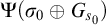 converges on the required vertices. Obviously, for any extension
$h\supseteq \sigma _{0}$
converges on the required vertices. Obviously, for any extension
$h\supseteq \sigma _{0}$
 and
$G\supseteq G_{s_{0}}$
and
$G\supseteq G_{s_{0}}$
 , we will have that
$\Psi (h\oplus G)$
, we will have that
$\Psi (h\oplus G)$
 also extends
$\Psi (\sigma _{0}\oplus G_{s_{0}})$
also extends
$\Psi (\sigma _{0}\oplus G_{s_{0}})$
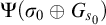 .
.
Suppose that
$\sigma _{l},\,s_{l}$
 have been defined such that
-
• $\sigma _{l}$
is a
$4l$
-coloring of
$\Phi (G_{s_{l}})$
, and -
• $s_{l}$
is the stage such that
$\Psi (\sigma _{l}\oplus G_{s_{l}})$
converges on the finitely many vertices of
$W_{m}$
enumerated thus far.


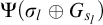

Let
$G_{s_{l}+1}$
 be the graph where the gadget
$W_{m}$
be the graph where the gadget
$W_{m}$
 has been extended to the
$l+1$
has been extended to the
$l+1$
 -th layer (see Section 2.1) based on the coloring
$\Psi (\sigma _{l}\oplus G_{s_{l}})$
-th layer (see Section 2.1) based on the coloring
$\Psi (\sigma _{l}\oplus G_{s_{l}})$
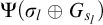 . Now let G be the union of
$G_{s_{l}+1}$
. Now let G be the union of
$G_{s_{l}+1}$
 with countably many isolated vertices and consider
$H=\Phi (G)$
with countably many isolated vertices and consider
$H=\Phi (G)$
 . By Lemma 3.1, there is a
$4(l+1)$
. By Lemma 3.1, there is a
$4(l+1)$
 -coloring
$h_{l+1}$
-coloring
$h_{l+1}$
 of H extending
$\sigma _{l}$
of H extending
$\sigma _{l}$
 . Clearly, as long as
$l<m\leq n+1$
. Clearly, as long as
$l<m\leq n+1$
 , there exists some finite stage
$s_{l+1}$
, there exists some finite stage
$s_{l+1}$
 such that
$\Psi (\sigma _{l+1}\oplus G_{s_{l+1}})$
such that
$\Psi (\sigma _{l+1}\oplus G_{s_{l+1}})$
 converges on the
$l+1$
converges on the
$l+1$
 -th layer of
$W_{m}$
-th layer of
$W_{m}$
 , where
$\sigma _{l+1}=h_{l+1}\restriction \Phi (G_{s_{l+1}})$
, where
$\sigma _{l+1}=h_{l+1}\restriction \Phi (G_{s_{l+1}})$
 . Furthermore, on the vertices up to the
$l^{th}$
. Furthermore, on the vertices up to the
$l^{th}$
 layer of
$W_{m}$
layer of
$W_{m}$
 ,
$\Psi (\sigma _{l+1}\oplus G_{s_{l+1}})$
,
$\Psi (\sigma _{l+1}\oplus G_{s_{l+1}})$
 agrees with
$\Psi (\sigma _{l}\oplus G_{s_{l}})$
agrees with
$\Psi (\sigma _{l}\oplus G_{s_{l}})$
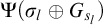 .
.
Repeat this procedure until
$W_{m}$
 has been successfully constructed and let
$h_{m}$
has been successfully constructed and let
$h_{m}$
 be the
$4m$
be the
$4m$
 -coloring of
$\Phi (G)$
-coloring of
$\Phi (G)$
 where G is the union of
$G_{s_{m-1}+1}$
where G is the union of
$G_{s_{m-1}+1}$
 with countably many isolated vertices. Since
$m\leq n+1$
with countably many isolated vertices. Since
$m\leq n+1$
 , then
$h_{m}$
, then
$h_{m}$
 is a
$4(n+1)$
is a
$4(n+1)$
 -coloring of
$H=\Phi (G)$
-coloring of
$H=\Phi (G)$
 . However,
$\Psi (h_{m}\oplus G)$
. However,
$\Psi (h_{m}\oplus G)$
 has the property that for each layer j of
$W_{m}$
has the property that for each layer j of
$W_{m}$
 ,
$\Psi (h_{m}\oplus G)$
,
$\Psi (h_{m}\oplus G)$
 colors the vertices of the
$j^{th}$
colors the vertices of the
$j^{th}$
 layer of
$W_{m}$
layer of
$W_{m}$
 in the same way as
$\Psi (\sigma _{j}\oplus G_{s_{j}})$
in the same way as
$\Psi (\sigma _{j}\oplus G_{s_{j}})$
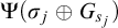 . In other words,
$W_{m}=W_{m}^{\Psi (h_{m}\oplus G)}$
. In other words,
$W_{m}=W_{m}^{\Psi (h_{m}\oplus G)}$
 (recall Notation 2.9) and thus cannot be
$(4n+i)$
(recall Notation 2.9) and thus cannot be
$(4n+i)$
 -colored by
$\Psi (h_{m}\oplus G)$
-colored by
$\Psi (h_{m}\oplus G)$
 .
.
Considering the proofs of Theorems 2.14, 2.16, and 2.18, we propose the following lemma that characterises the existence of a uniform reduction of a
${\mathtt {DNR}}$
 principle to
${\mathtt {COL}}$
principle to
${\mathtt {COL}}$
 principle as a (finite) graph theoretic property.
Lemma 3.4. The following are equivalent:
-
(1) ${\mathtt {DNR}}(k){\leq _{\mathsf {sW}}}{\mathtt {COL}}(n)$
. -
(2) ${\mathtt {DNR}}(k){\leq _{\mathsf {W}}} {\mathtt {COL}}(n)$
. -
(3) There exists finite planar graph $G,G_{0},G_{1},\dots ,G_{k-1}$
such that for each
$i<k,\,G_{i}\supseteq G$
and for any n-coloring h of G, there is some
$i<k$
such that h does not extend to an n-coloring of
$G_{i}$
.






Proof. (1) implies that (2) is obvious. We first prove the implication from (2) to (3). Suppose that
${\mathtt {DNR}}(k){\leq _{\mathsf {W}}} {\mathtt {COL}}(n)$
 . Then there exists
$\Phi ,\Psi $
. Then there exists
$\Phi ,\Psi $
 such that for any oracle f,
$\Phi (f)=H$
such that for any oracle f,
$\Phi (f)=H$
 is a countable planar graph and given an n-coloring h of H,
$\Psi (h\oplus f)=g$
is a countable planar graph and given an n-coloring h of H,
$\Psi (h\oplus f)=g$
 satisfies
${\mathtt {DNR}}(k)$
satisfies
${\mathtt {DNR}}(k)$
 .
.
Consider a tree T defined as follows. T contains elements of the form
$\langle \sigma ,f\rangle $
 where
$\sigma $
where
$\sigma $
 is a finite n-ary string and f is a finite binary string (satisfying the conditions below). In addition, the ordering between two elements is given by
$\langle \sigma ,f\rangle \leq \langle \sigma ',f'\rangle $
is a finite n-ary string and f is a finite binary string (satisfying the conditions below). In addition, the ordering between two elements is given by
$\langle \sigma ,f\rangle \leq \langle \sigma ',f'\rangle $
 iff
$\sigma \subseteq \sigma '$
iff
$\sigma \subseteq \sigma '$
 and
$f\subseteq f'$
and
$f\subseteq f'$
 . Now generate T recursively as follows:
-
• $\langle \rangle \in T$
. -
• If $\langle \sigma ,f\rangle \in T$
, then
$\langle \tau ,f^{\frown }j\rangle \in T$
provided
$\tau \supseteq \sigma $
and
$\tau $
is a valid n-coloring of
$\Phi (f^{\frown }j)$
.Footnote
6
We also require that
$\tau $
has length the number of vertices enumerated by
$\Phi (f^{\frown }j)$
.





Given any n-coloring
$\sigma $
 of
$\Phi (f)$
of
$\Phi (f)$
 , there are only a finite number of colorings
$\tau \supseteq \sigma $
, there are only a finite number of colorings
$\tau \supseteq \sigma $
 that colors
$\Phi (f^{\frown }j)$
that colors
$\Phi (f^{\frown }j)$
 . Furthermore, such
$\tau $
. Furthermore, such
$\tau $
 can be computably determined. Therefore, T is a computable finite branching tree. For a given e, define the subtree
$T_{e}\subseteq T$
can be computably determined. Therefore, T is a computable finite branching tree. For a given e, define the subtree
$T_{e}\subseteq T$
 as containing all nodes
$\langle \sigma ,f\rangle \in T$
as containing all nodes
$\langle \sigma ,f\rangle \in T$
 for which
$\Psi (\sigma \oplus f)(e)[|f|]{\uparrow }$
for which
$\Psi (\sigma \oplus f)(e)[|f|]{\uparrow }$
 . Since T is finite branching, if
$T_{e}\subseteq T$
. Since T is finite branching, if
$T_{e}\subseteq T$
 is infinite, then there must be a path through
$T_{e}$
is infinite, then there must be a path through
$T_{e}$
 . Let this path be given by
$\langle \sigma ,f\rangle $
. Let this path be given by
$\langle \sigma ,f\rangle $
 , where f is an infinite binary string. Observe that
$\sigma ,f$
, where f is an infinite binary string. Observe that
$\sigma ,f$
 has the following properties:
-
• Since $\Phi $
is total, then
$\Phi (f)$
must be a countable planar graph. Therefore,
$\sigma $
must also be of infinite length by the second condition in the definition of T. Furthermore,
$\sigma $
is an n-coloring of
$\Phi (f)$
. -
• For each s, $\Psi (\sigma \oplus f)(e)[s]{\uparrow }$
. That is,
$\Psi (\sigma \oplus f)$
is not a total function and cannot possibly satisfy
${\mathtt {DNR}}(k)$
.





This contradicts the assumption that
$\Phi ,\Psi $
 witnesses
${\mathtt {DNR}}(k){\leq _{\mathsf {W}}} {\mathtt {COL}}(n)$
witnesses
${\mathtt {DNR}}(k){\leq _{\mathsf {W}}} {\mathtt {COL}}(n)$
 . Thus
$T_{e}$
. Thus
$T_{e}$
 must be finite. In other words, there can only be finitely many nodes of T for which
$\Psi (\sigma \oplus f)(e)[|f|]{\uparrow }$
must be finite. In other words, there can only be finitely many nodes of T for which
$\Psi (\sigma \oplus f)(e)[|f|]{\uparrow }$
 . Therefore, there is a finite s, such that for every f of length s, and every possible n-coloring
$\sigma $
. Therefore, there is a finite s, such that for every f of length s, and every possible n-coloring
$\sigma $
 of
$\Phi (f),\,\Psi (\sigma \oplus f)(e)[s]{\downarrow }$
of
$\Phi (f),\,\Psi (\sigma \oplus f)(e)[s]{\downarrow }$
 . Furthermore, we note that such an s can be found recursively in e. For any given input e, we denote such an s as
$s_{e}$
. Furthermore, we note that such an s can be found recursively in e. For any given input e, we denote such an s as
$s_{e}$
 .
.
Consider the partial computable function
$\psi (x)$
 defined as follows. On any input x,
$\psi $
defined as follows. On any input x,
$\psi $
 outputs the number of consecutive zeros between the first two non-zero bits of its oracle f. Let the index of
$\psi $
outputs the number of consecutive zeros between the first two non-zero bits of its oracle f. Let the index of
$\psi $
 be e, that is,
$\psi ^{f}=\varphi _{e}^{f}$
be e, that is,
$\psi ^{f}=\varphi _{e}^{f}$
 for any f. Fix such an e and let
$G=\Phi (0^{s_{e}})$
for any f. Fix such an e and let
$G=\Phi (0^{s_{e}})$
 . Note that there are only finitely many possible n-colorings of G. We list these colorings as
$\sigma _{0},\sigma _{1},\dots ,\sigma _{m}$
. Note that there are only finitely many possible n-colorings of G. We list these colorings as
$\sigma _{0},\sigma _{1},\dots ,\sigma _{m}$
 . For each
$i<k$
. For each
$i<k$
 , let
$r_{i}\geq 0$
, let
$r_{i}\geq 0$
 be the least number satisfying the following. For any
$l\leq m$
be the least number satisfying the following. For any
$l\leq m$
 , if
$\Psi (\sigma _{l}\oplus 0^{s_{e}})(e)[s_{e}]=i$
, if
$\Psi (\sigma _{l}\oplus 0^{s_{e}})(e)[s_{e}]=i$
 (note that
$\Psi (\sigma _{l}\oplus 0^{s_{e}})(e)[s_{e}]{\downarrow }$
(note that
$\Psi (\sigma _{l}\oplus 0^{s_{e}})(e)[s_{e}]{\downarrow }$
 by choice of
$s_{e}$
by choice of
$s_{e}$
 ), then for any
$\tau \supseteq \sigma _{l},\,\langle \tau ,0^{s_{e}}10^{i}10^{r_{i}}\rangle \notin T$
), then for any
$\tau \supseteq \sigma _{l},\,\langle \tau ,0^{s_{e}}10^{i}10^{r_{i}}\rangle \notin T$
 .
.
Suppose for a contradiction that
$r_{i}$
 does not exist. That is, for every
$j\in \omega $
does not exist. That is, for every
$j\in \omega $
 , there exists some
$\tau \supseteq \sigma _{l}$
, there exists some
$\tau \supseteq \sigma _{l}$
 such that
$\langle \tau ,0^{s_{e}}10^{i}10^{j}\rangle \in T$
such that
$\langle \tau ,0^{s_{e}}10^{i}10^{j}\rangle \in T$
 . Then, the subtree consisting of nodes
$\langle \tau ,0^{s_{e}}10^{i}10^{j}\rangle $
. Then, the subtree consisting of nodes
$\langle \tau ,0^{s_{e}}10^{i}10^{j}\rangle $
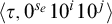 must be infinite, and thus has a path, say
$\langle \hat {\tau },0^{s_{e}}10^{i}10^{\omega }\rangle $
must be infinite, and thus has a path, say
$\langle \hat {\tau },0^{s_{e}}10^{i}10^{\omega }\rangle $
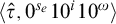 , where
$\hat {\tau }\supseteq \sigma _{l}$
, where
$\hat {\tau }\supseteq \sigma _{l}$
 . As explained previously, since
$\Phi $
. As explained previously, since
$\Phi $
 is total, then
$\hat {\tau }$
is total, then
$\hat {\tau }$
 must be of infinite length and an n-coloring of
$\Phi (0^{s_{e}}10^{i}10^{\omega })$
must be of infinite length and an n-coloring of
$\Phi (0^{s_{e}}10^{i}10^{\omega })$
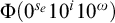 . Hence, we obtain that

Contradicting the assumption that
$\Phi ,\Psi $
 witnesses
${\mathtt {DNR}}(k){\leq _{\mathsf {W}}} {\mathtt {COL}}(n)$
witnesses
${\mathtt {DNR}}(k){\leq _{\mathsf {W}}} {\mathtt {COL}}(n)$
 . Thus
$r_{i}$
. Thus
$r_{i}$
 must exist; there is some finite depth such that the subtree extending
$\langle \sigma _{l},0^{s_{e}}10^{i}1\rangle $
must exist; there is some finite depth such that the subtree extending
$\langle \sigma _{l},0^{s_{e}}10^{i}1\rangle $
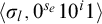 is witnessed to be finite. For each
$i<k$
is witnessed to be finite. For each
$i<k$
 , define
$G_{i}=\Phi (0^{s_{e}}10^{i}10^{r_{i}})$
, define
$G_{i}=\Phi (0^{s_{e}}10^{i}10^{r_{i}})$
 . Evidently, for any coloring h of G,
$h=\sigma _{l}$
. Evidently, for any coloring h of G,
$h=\sigma _{l}$
 for some l. Let
$\Psi (\sigma _{l}\oplus 0^{s_{e}})(e)=i$
for some l. Let
$\Psi (\sigma _{l}\oplus 0^{s_{e}})(e)=i$
 . Then h cannot extend to an n-coloring of
$G_{i}$
. Then h cannot extend to an n-coloring of
$G_{i}$
 , otherwise there must be some
$\tau $
, otherwise there must be some
$\tau $
 such that
$\langle \tau ,0^{s_{e}}10^{i}10^{r_{i}}\rangle \in T$
such that
$\langle \tau ,0^{s_{e}}10^{i}10^{r_{i}}\rangle \in T$
 where
$\tau \supseteq \sigma _{l}$
where
$\tau \supseteq \sigma _{l}$
 .
.
It remains to prove the implication from (3) to (1). Suppose that there is some finite planar graph H, and finite planar extensions of H,
$H_{0},H_{1},\dots ,H_{k-1}$
 such that for any k-coloring h of H, there is some
$i<k$
such that for any k-coloring h of H, there is some
$i<k$
 where h does not extend to an n-coloring of
$H_{i}$
where h does not extend to an n-coloring of
$H_{i}$
 . The idea is to build G in diagonalisation components, one for each e. Each component will initially consist of H and potentially be extended to one of the
$H_{i}$
. The idea is to build G in diagonalisation components, one for each e. Each component will initially consist of H and potentially be extended to one of the
$H_{i}$
 . It is important to note that H and
$H_{i}$
. It is important to note that H and
$H_{i}$
 are completely independent of f (the oracle to
${\mathtt {DNR}}(k)$
are completely independent of f (the oracle to
${\mathtt {DNR}}(k)$
 ), and thus we may fix (beforehand) some encoding of the initial vertices of H in the
$e^{th}$
), and thus we may fix (beforehand) some encoding of the initial vertices of H in the
$e^{th}$
 component.
For any oracle f, define G as follows.
-
Stage s: Enumerate a new copy of H into G and refer to this as the initial part of the $s^{th}$
component. If
$\varphi _{e}^{f}(e)[s]{\downarrow }$
for some
$e<s$
and the
$e^{th}$
component has not yet acted, then extend H to
$H_{i}$
provided
$\varphi _{e}^{f}(e)[s]=i<k$
. Once H has been extended to
$H_{i}$
, we say that the
$e^{th}$
component has acted.





Now let h be any n-coloring of G as defined above. In order to define
$\Psi (h)(e)$
 , we consider the
$e^{th}$
, we consider the
$e^{th}$
 component. Wait for h to converge on all the vertices of H in the
$e^{th}$
component. Wait for h to converge on all the vertices of H in the
$e^{th}$
 component. Once it does so, we know that there exists some i such that h cannot be extended to an n-coloring of
$H_{i}$
component. Once it does so, we know that there exists some i such that h cannot be extended to an n-coloring of
$H_{i}$
 . Since there are only finitely many possible colorings of each
$H_{j}$
. Since there are only finitely many possible colorings of each
$H_{j}$
 for
$j<k$
for
$j<k$
 , we can find such an i computably in h. If there are multiple such i, pick the least one and let
$\Psi (h)(e)=i$
, we can find such an i computably in h. If there are multiple such i, pick the least one and let
$\Psi (h)(e)=i$
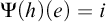 . Then
$\Psi (h)(e){\downarrow }\neq \varphi _{e}^{f}(e)$
. Then
$\Psi (h)(e){\downarrow }\neq \varphi _{e}^{f}(e)$
 , otherwise h cannot be a n-coloring of G. In particular, it fails to color the
$e^{th}$
, otherwise h cannot be a n-coloring of G. In particular, it fails to color the
$e^{th}$
 component of G.
Applying Lemma 3.4, we can easily obtain that for any planar graph G and any number of planar extensions
$G_{0},\dots ,G_{k}$
 , there is an
$8$
, there is an
$8$
 -coloring of G (use only four colors) that can be extended to an
$8$
-coloring of G (use only four colors) that can be extended to an
$8$
 coloring of any
$G_{i}$
coloring of any
$G_{i}$
 (Lemma 3.1). Thus, for any
$k,\,{\mathtt {DNR}}(k){\not \!\!{\leq _{\mathsf {W}}}}{\mathtt {COL}}(8)$
(Lemma 3.1). Thus, for any
$k,\,{\mathtt {DNR}}(k){\not \!\!{\leq _{\mathsf {W}}}}{\mathtt {COL}}(8)$
 . This is not too surprising considering the stronger result in Theorem 3.2. We can however obtain an improvement to the result in Theorem 3.2, in the sense that the non-uniformity is necessary even for
${\mathtt {RCA}_{0}}+{\mathtt {COL}}(7)\,\vdash\, {{\mathtt {WKL}}}$
. This is not too surprising considering the stronger result in Theorem 3.2. We can however obtain an improvement to the result in Theorem 3.2, in the sense that the non-uniformity is necessary even for
${\mathtt {RCA}_{0}}+{\mathtt {COL}}(7)\,\vdash\, {{\mathtt {WKL}}}$
 .
.
Theorem 3.5.
${\mathtt {DNR}}(2){\not \!\!{\leq _{\mathsf {W}}}}{\mathtt {COL}}(7)$
 .
.
Proof. By Lemma 3.4, it suffices to show that for any finite planar graph G, and finite planar extensions
$G_{0},G_{1}$
 , there exists g, a
$7$
, there exists g, a
$7$
 -coloring of G such that g extends to a
$7$
-coloring of G such that g extends to a
$7$
 -coloring of both
$G_{0}$
-coloring of both
$G_{0}$
 and
$G_{1}$
and
$G_{1}$
 . Since
$G_{0}$
. Since
$G_{0}$
 and
$G_{1}$
and
$G_{1}$
 are both finite planar extensions of G, then it must be that there are
$4$
are both finite planar extensions of G, then it must be that there are
$4$
 -colorings
$g_{0},g_{1}$
-colorings
$g_{0},g_{1}$
 of
$G_{0},G_{1}$
of
$G_{0},G_{1}$
 , respectively. Now we construct a
$7$
, respectively. Now we construct a
$7$
 -coloring, h, of G as follows:

It follows that
$h(v)<7$
 for each v. We check that h is a
$7$
for each v. We check that h is a
$7$
 -coloring of G. Let
$u,v\in G$
-coloring of G. Let
$u,v\in G$
 be arbitrarily chosen such that
$\{u,v\}\in E_{G}$
be arbitrarily chosen such that
$\{u,v\}\in E_{G}$
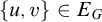 . Suppose to the contrary that
$h(u)=h(v)$
. Suppose to the contrary that
$h(u)=h(v)$
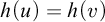 . Then either
$g_{0}(u)=g_{0}(v)$
. Then either
$g_{0}(u)=g_{0}(v)$
 or
$g_{1}(u)+3=g_{1}(v)+3$
or
$g_{1}(u)+3=g_{1}(v)+3$
 , in either cases, it implies that
$g_{0}$
, in either cases, it implies that
$g_{0}$
 or
$g_{1}$
or
$g_{1}$
 is not a coloring of G, which cannot be the case. since
$G\subset G_{i}$
is not a coloring of G, which cannot be the case. since
$G\subset G_{i}$
 for each
$i<2$
for each
$i<2$
 . Thus h is a
$7$
. Thus h is a
$7$
 -coloring of G. It remains to show that h can be extended to a
$7$
-coloring of G. It remains to show that h can be extended to a
$7$
 -coloring
$h_{i}$
-coloring
$h_{i}$
 of
$G_{i}$
of
$G_{i}$
 , for each
$i=0,1$
, for each
$i=0,1$
 ,
,

and

It remains to check that each
$h_{i}$
 is a
$7$
is a
$7$
 -coloring of
$G_{i}$
-coloring of
$G_{i}$
 . We first check for
$i=0$
. We first check for
$i=0$
 . Let
$u,v\in G_{0}$
. Let
$u,v\in G_{0}$
 such that
$\{u,v\}\in E_{G_{0}}$
such that
$\{u,v\}\in E_{G_{0}}$
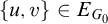 . The case for
$u,v\in G$
. The case for
$u,v\in G$
 has already been checked, since h is a valid coloring of G. Also, if both
$u,v\in G_{0}\setminus G$
has already been checked, since h is a valid coloring of G. Also, if both
$u,v\in G_{0}\setminus G$
 ,
$h_{0}(u)=g_{0}(u)\neq g_{0}(v)=h_{0}(v)$
,
$h_{0}(u)=g_{0}(u)\neq g_{0}(v)=h_{0}(v)$
 . So we may assume without loss of generality that
$u\in G$
. So we may assume without loss of generality that
$u\in G$
 and
$v\in G_{0}\setminus G$
and
$v\in G_{0}\setminus G$
 with the property that
$h_{0}(u)=h_{0}(v)$
with the property that
$h_{0}(u)=h_{0}(v)$
 . Following the definition of
$h_{0}$
. Following the definition of
$h_{0}$
 , since
$v\in G_{0}\setminus G$
, since
$v\in G_{0}\setminus G$
 , then
$h_{0}(v)<4$
, then
$h_{0}(v)<4$
 . Then we must also have that
$h_{0}(u)<4$
. Then we must also have that
$h_{0}(u)<4$
 . It is evident that if
$h_{0}(u)=0,1,2$
. It is evident that if
$h_{0}(u)=0,1,2$
 , then
$h_{0}(u)=g_{0}(u)$
, then
$h_{0}(u)=g_{0}(u)$
 . On the other hand, if
$h_{0}(u)=3$
. On the other hand, if
$h_{0}(u)=3$
 , then it can only be that
$g_{0}(u)=3$
, then it can only be that
$g_{0}(u)=3$
 and
$g_{1}(u)=0$
and
$g_{1}(u)=0$
 . In particular, if
$h_{0}(u)<4$
. In particular, if
$h_{0}(u)<4$
 , then
$h_{0}(u)=g_{0}(u)$
, then
$h_{0}(u)=g_{0}(u)$
 . Therefore, we obtain
$g_{0}(v)=h_{0}(v)=h_{0}(u)=g_{0}(u)$
. Therefore, we obtain
$g_{0}(v)=h_{0}(v)=h_{0}(u)=g_{0}(u)$
 , contradicting the fact that
$g_{0}$
, contradicting the fact that
$g_{0}$
 is a
$4$
is a
$4$
 -coloring of
$G_{0}$
-coloring of
$G_{0}$
 .
.
For the case
$i=1$
 , let
$u,v\in G_{1}$
, let
$u,v\in G_{1}$
 be such that
$\{u,v\}\in E_{G_{1}}$
be such that
$\{u,v\}\in E_{G_{1}}$
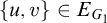 . Once again, if both
$u,v\in G$
. Once again, if both
$u,v\in G$
 or both
$u,v\notin G$
or both
$u,v\notin G$
 , then it must be that
$h_{1}(u)\neq h_{1}(v)$
, then it must be that
$h_{1}(u)\neq h_{1}(v)$
 , otherwise
$g_{0}$
, otherwise
$g_{0}$
 or
$g_{1}$
or
$g_{1}$
 , respectively, fails to be a coloring. Thus, without loss of generality, we may assume that
$u\in G$
, respectively, fails to be a coloring. Thus, without loss of generality, we may assume that
$u\in G$
 and
$v\notin G$
and
$v\notin G$
 such that
$h_{1}(u)=h_{1}(v)$
such that
$h_{1}(u)=h_{1}(v)$
 . This implies that
$h_{1}(u)=3=h_{1}(v)$
. This implies that
$h_{1}(u)=3=h_{1}(v)$
 . Applying the definition of h allows us to conclude that if
$h(u)=3$
. Applying the definition of h allows us to conclude that if
$h(u)=3$
 , then
$g_{1}(u)=0$
, then
$g_{1}(u)=0$
 . Since
$h_{1}(v)=3=g_{1}(v)+3$
. Since
$h_{1}(v)=3=g_{1}(v)+3$
 , we obtain
$g_{1}(u)=g_{1}(v)$
, we obtain
$g_{1}(u)=g_{1}(v)$
 , contradicting the assumption that
$g_{1}$
, contradicting the assumption that
$g_{1}$
 is a coloring.
Thus, for any
$G,G_{0},G_{1}$
 where
$G_{i}\supset G$
where
$G_{i}\supset G$
 for each
$i<2$
for each
$i<2$
 , there is some
$7$
, there is some
$7$
 -coloring h of G such that h can be extended to a
$7$
-coloring h of G such that h can be extended to a
$7$
 -coloring of
$G_{0}$
-coloring of
$G_{0}$
 and
$G_{1}$
and
$G_{1}$
 . Then by Lemma 3.4,
${\mathtt {DNR}}(2){\not \!\!{\leq _{\mathsf {W}}}}{\mathtt {COL}}(7)$
. Then by Lemma 3.4,
${\mathtt {DNR}}(2){\not \!\!{\leq _{\mathsf {W}}}}{\mathtt {COL}}(7)$
 .
.
3.2 Extending colorings
The proofs of Theorem 3.3 and Lemma 3.4 seem to suggest that the question of Weihrauch reducibility between the coloring principles and
${\mathtt {DNR}}$
 boils down to the ability to extend colorings. The task now is to prove an analogous result as in Lemma 3.1 for the principles
${\mathtt {ConnCOL}}$
boils down to the ability to extend colorings. The task now is to prove an analogous result as in Lemma 3.1 for the principles
${\mathtt {ConnCOL}}$
 and
${\mathtt {COL}}^{*}$
and
${\mathtt {COL}}^{*}$
 . It turns out that with the additional assumptions, we have a slightly stronger result for
${\mathtt {ConnCOL}}$
. It turns out that with the additional assumptions, we have a slightly stronger result for
${\mathtt {ConnCOL}}$
 (Lemma 3.6) and
${\mathtt {COL}}^{*}$
(Lemma 3.6) and
${\mathtt {COL}}^{*}$
 (Lemma 3.12).
Lemma 3.6. For a given finite connected planar graph G, and a countable connected planar graph
$G'\supset G$
 , if c is a k-coloring (
$k\geq 3$
, if c is a k-coloring (
$k\geq 3$
 ) of G, then there is some
$\hat {c}$
) of G, then there is some
$\hat {c}$
 a
$k+3$
a
$k+3$
 -coloring of
$G'$
-coloring of
$G'$
 that extends c.
We follow the proof of Theorem 5 in [Reference Bean1] closely. In the article, the author considers recursive colorings of connected highly recursive graphs; graphs where
$N(v)$
 , the set of neighbours of a vertex v, are uniformly computable. The same technique can essentially be applied assuming that we have access to
$N(v)$
, the set of neighbours of a vertex v, are uniformly computable. The same technique can essentially be applied assuming that we have access to
$N(v)$
 . We note here that every computable graph is
$\emptyset '$
. We note here that every computable graph is
$\emptyset '$
 -highly recursive. In any case, we do not require that the colorings c and
$\hat {c}$
-highly recursive. In any case, we do not require that the colorings c and
$\hat {c}$
 be effective in any way. One might wonder if the proof would work to show an analogous result for the basic coloring principle. Unfortunately, this technique seems to fail in the case that G has infinitely many disconnected components because we no longer are able to guarantee that the ‘layers’ (to be specified in the proof) are sufficiently disjoint.
Proof of Lemma 3.6
Let
$G_{0}=G$
 . Iteratively define
$G_{n+1}$
. Iteratively define
$G_{n+1}$
 as the induced subgraph of
$G'$
as the induced subgraph of
$G'$
 such that
$V_{G_{n+1}}=\bigcup _{v\in V_{G_{n}}}N(v)\cup G_{n}$
such that
$V_{G_{n+1}}=\bigcup _{v\in V_{G_{n}}}N(v)\cup G_{n}$
 . Also define
$\overline {G_{0}}=G_{0}$
. Also define
$\overline {G_{0}}=G_{0}$
 , and
$\overline {G_{n+1}}=G_{n+1}\setminus G_{n}$
, and
$\overline {G_{n+1}}=G_{n+1}\setminus G_{n}$
 . Note that the vertex sets of the graphs
$\overline {G_{n}}$
. Note that the vertex sets of the graphs
$\overline {G_{n}}$
 are mutually disjoint, and form a partition of
$G'$
are mutually disjoint, and form a partition of
$G'$
 . Furthermore, for any n,
-
• $N\left (V_{\overline {G_{n}}}\right )= V_{\overline {G_{n-1}}}\cup V_{\overline {G_{n+1}}}$
. -
• $N\left (V_{\overline {G_{n}}}\right )\cap V_{\overline {G_{m}}}=\emptyset $
and
$N\left (V_{\overline {G_{m}}}\right )\cap V_{\overline {G_{n}}}=\emptyset $
, for any m where
$\left |m-n\right |>1$
.




We will attempt to
$k+3$
 -color
$G'$
-color
$G'$
 as follows. First we k-color
$G_{0}=G$
as follows. First we k-color
$G_{0}=G$
 using c. Now we
$3$
using c. Now we
$3$
 -color each subsequent layer
$\overline {G_{n}}$
-color each subsequent layer
$\overline {G_{n}}$
 where
$n>0$
where
$n>0$
 . If n is odd, then we use the colors
$k,k+1,k+2$
. If n is odd, then we use the colors
$k,k+1,k+2$
 , otherwise we use the colors
$0,1,2$
, otherwise we use the colors
$0,1,2$
 . The properties listed above ensure that the even and odd layers are ‘sufficiently’ disjoint, and ensures that this strategy results in a
$k+3$
. The properties listed above ensure that the even and odd layers are ‘sufficiently’ disjoint, and ensures that this strategy results in a
$k+3$
 -coloring of
$G'$
-coloring of
$G'$
 . We provide the details below.
For each
$n>0$
 , define an equivalence relation on the vertices of
$G_{n}$
, define an equivalence relation on the vertices of
$G_{n}$
 ;
$u\sim _{n}v$
;
$u\sim _{n}v$
 iff
$u,v\in G_{n-1}$
iff
$u,v\in G_{n-1}$
 . Then let
$H_{n}$
. Then let
$H_{n}$
 be the graph with vertices representing the distinct equivalence classes of
$G_{n}$
be the graph with vertices representing the distinct equivalence classes of
$G_{n}$
 (denoted
$\mathbf {u}$
(denoted
$\mathbf {u}$
 ) and having edge relation
$\{\mathbf {u},\mathbf {v}\}\in E_{H_{n}}$
) and having edge relation
$\{\mathbf {u},\mathbf {v}\}\in E_{H_{n}}$
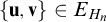 iff there exists
$u\in \mathbf {u}$
iff there exists
$u\in \mathbf {u}$
 and
$v\in \mathbf {v}$
and
$v\in \mathbf {v}$
 such that
$\{u,v\}\in E_{G_{n}}$
such that
$\{u,v\}\in E_{G_{n}}$
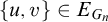 .
$H_{n}$
.
$H_{n}$
 can then be seen as the graph
$\overline {G_{n}}$
can then be seen as the graph
$\overline {G_{n}}$
 with an additional vertex say
$w_{n}$
with an additional vertex say
$w_{n}$
 (representing the equivalence class containing all the vertices of
$G_{n-1}$
(representing the equivalence class containing all the vertices of
$G_{n-1}$
 ) that is connected to all other vertices in
$\overline {G_{n}}$
) that is connected to all other vertices in
$\overline {G_{n}}$
 . We first prove that
$H_{n}$
. We first prove that
$H_{n}$
 is indeed planar.
Suppose to the contrary that
$H_{n}$
 is not planar, then
$H_{n}$
is not planar, then
$H_{n}$
 must have
$K_{5}$
must have
$K_{5}$
 or
$K_{3,3}$
or
$K_{3,3}$
 as a minor. That is, there is some finite sequence of contractions that can be used to obtain a graph isomorphic to
$K_{3,3}$
as a minor. That is, there is some finite sequence of contractions that can be used to obtain a graph isomorphic to
$K_{3,3}$
 or
$K_{5}$
or
$K_{5}$
 . If such a sequence of contractions do not include the vertex
$w_{n}$
. If such a sequence of contractions do not include the vertex
$w_{n}$
 , then we note that the same sequence of contractions can be done on
$G_{n}$
, then we note that the same sequence of contractions can be done on
$G_{n}$
 to show that
$G_{n}$
to show that
$G_{n}$
 is not planar. We may thus suppose that the sequence of contractions does include
$w_{n}$
is not planar. We may thus suppose that the sequence of contractions does include
$w_{n}$
 . In particular, there are two vertices
$u,v\in \overline {G_{n}}$
. In particular, there are two vertices
$u,v\in \overline {G_{n}}$
 such that
$\{u,w_{n}\},\{v,w_{n}\}\in E_{H_{n}}$
such that
$\{u,w_{n}\},\{v,w_{n}\}\in E_{H_{n}}$
 . But that means that there exists
$u^{*},v^{*}\in G_{n-1}$
. But that means that there exists
$u^{*},v^{*}\in G_{n-1}$
 where
$\{u,u^{*}\},\{v,v^{*}\}\in E_{G_{n}}$
where
$\{u,u^{*}\},\{v,v^{*}\}\in E_{G_{n}}$
 . Since
$G_{n}$
. Since
$G_{n}$
 is connected, then
$u^{*},v^{*}$
is connected, then
$u^{*},v^{*}$
 must be connected via some finite path. In other words, by replacing the contraction which removes
$w_{n}$
must be connected via some finite path. In other words, by replacing the contraction which removes
$w_{n}$
 with this finite sequence of contractions that removes the path between
$u^{*}$
with this finite sequence of contractions that removes the path between
$u^{*}$
 and
$v^{*}$
and
$v^{*}$
 , we are again able to obtain a graph that is isomorphic to
$K_{3,3}$
, we are again able to obtain a graph that is isomorphic to
$K_{3,3}$
 or
$K_{5}$
or
$K_{5}$
 , contradicting the assumption that
$G_{n}$
, contradicting the assumption that
$G_{n}$
 is planar.
Since
$H_{n}$
 is planar, then
$H_{n}$
is planar, then
$H_{n}$
 can be
$4$
can be
$4$
 -colored. Furthermore, in any coloring of
$H_{n}$
-colored. Furthermore, in any coloring of
$H_{n}$
 ,
$w_{n}$
,
$w_{n}$
 must be a different color from any of the other vertices in
$\overline {G_{n}}$
must be a different color from any of the other vertices in
$\overline {G_{n}}$
 . We may thus assume that the
$4$
. We may thus assume that the
$4$
 -coloring h of
$H_{n}$
-coloring h of
$H_{n}$
 assigns the colors
$0,1,2$
assigns the colors
$0,1,2$
 to the vertices in
$\overline {G_{n}}$
to the vertices in
$\overline {G_{n}}$
 and the color
$3$
and the color
$3$
 to
$w_{n}$
to
$w_{n}$
 . Then given a
$k+3$
. Then given a
$k+3$
 -coloring g of
$G_{n-1}$
-coloring g of
$G_{n-1}$
 , we extend it to a
$k+3$
, we extend it to a
$k+3$
 -coloring
$g'$
-coloring
$g'$
 of
$G_{n}$
of
$G_{n}$
 as follows:

Then repeat the process inductively to obtain a coloring for
$G'$
 . To see that it is indeed a
$k+3$
. To see that it is indeed a
$k+3$
 -coloring, we use the fact that for any n, for any
$u\in \overline {G_{n}}$
-coloring, we use the fact that for any n, for any
$u\in \overline {G_{n}}$
 and any
$v\in \overline {G_{n+2}}$
and any
$v\in \overline {G_{n+2}}$
 ,
$\{u,v\}\notin E$
,
$\{u,v\}\notin E$
 . Together with the fact that all vertices in the odd layers are colored using
$k,k+1,k+2$
. Together with the fact that all vertices in the odd layers are colored using
$k,k+1,k+2$
 while vertices in the even layers utilising colors
$<k$
while vertices in the even layers utilising colors
$<k$
 , we obtain that the coloring defined is indeed a
$k+3$
, we obtain that the coloring defined is indeed a
$k+3$
 -coloring.
In order to prove a similar lemma for
${\mathtt {COL}}^{*}$
 , it should be clear that we have to utilise the plane diagram (recall Definition 1.3) in some way. The rough idea is to consider good colorings (to be defined later) of the graph and show that they can be extended. This class of colorings is characterised by their behaviour on the faces of a diagram. Since we need to consider the plane diagrams, a notion for diagram extensions is required.
Definition 3.7. Let D be a plane diagram of G. A plane diagram
$D'$
 is an extension of D, written
$D'\supseteq D$
is an extension of D, written
$D'\supseteq D$
 if the following holds:
-
• $D'$
is a plane diagram of
$G'\supseteq G$
(recall this means that G is an induced subgraph of
$G'$
). -
• $D'$
restricted to G is exactly D.


Intuitively, this means that if a diagram D has exhibited that two vertices are not adjacent, then no extension of D can add an edge between the two vertices. Using this property, once we know how D embeds the vertices and edges of G into
${\mathbb {R}}^{2}$
 , then we have a good idea about which vertices can later share some common neighbour. Using this information, we can be more efficient on the usage of colors.
Fact 3.8. Given a finite graph G with plane diagram D,
${\mathbb {R}}^{2}\setminus D$
 is a disjoint union
$\bigsqcup _{i<m}U_{i}$
is a disjoint union
$\bigsqcup _{i<m}U_{i}$
 where each
$U_{i}$
where each
$U_{i}$
 is homeomorphic to an open disc with at most finitely many holes.
Proof sketch
Since D can be expressed as a union of finitely many compact line segments (each representing an edge) such that two distinct line segments possibly intersect only at the endpoints, an inductive argument can be done to show the desired result. We present some representative cases in Figure 10. Each subdiagram corresponds to some configuration of how the
$n+1$
 -th line segment could be positioned relative to one of the connected components of
${\mathbb {R}}^{2}$
-th line segment could be positioned relative to one of the connected components of
${\mathbb {R}}^{2}$
 without the first n many line segments. It follows that in each case, the hypothesis is still satisfied after removing the
$n+1$
without the first n many line segments. It follows that in each case, the hypothesis is still satisfied after removing the
$n+1$
 -th line.
Some possible configurations of a line segment and a connected component.

Consider some extension
$D'\supseteq D$
 . Let
$u,v$
. Let
$u,v$
 be two vertices which are adjacent and are added only in
$D'$
be two vertices which are adjacent and are added only in
$D'$
 . Applying Fact 3.8, we can conclude that
$u,v$
. Applying Fact 3.8, we can conclude that
$u,v$
 are both within the same connected component. Otherwise,
$D'$
are both within the same connected component. Otherwise,
$D'$
 cannot be a planar diagram as the embedding of the edge between
$u,v$
cannot be a planar diagram as the embedding of the edge between
$u,v$
 necessarily crosses some part of D. Intuitively, the connected components of D influence which vertices added later may be adjacent. This motivates the following definition.
Definition 3.9. Let G be a finite planar graph with plane diagram D and let
$\{U_{i}\}_{i\leq m}$
 be a partition of
${\mathbb {R}}^{2}\setminus D$
be a partition of
${\mathbb {R}}^{2}\setminus D$
 such that each
$U_{i}$
such that each
$U_{i}$
 is an open connected region. Then we say that c is a good
$(3k+1)$
is an open connected region. Then we say that c is a good
$(3k+1)$
 -coloring of D if c is a
$(3k+1)$
-coloring of D if c is a
$(3k+1)$
 -coloring of G and for each
$U_{i}$
-coloring of G and for each
$U_{i}$
 , c uses
$3k$
, c uses
$3k$
 colors to color all the vertices on
$\partial U_{i}$
colors to color all the vertices on
$\partial U_{i}$
 . Note that the
$3k$
. Note that the
$3k$
 colors can differ between different
$U_{i}$
colors can differ between different
$U_{i}$
 .
.
In what follows, since we will be working mainly with the diagrams, we shall simply write
$u\in X$
 for some
$X\subseteq {\mathbb {R}}^{2}$
for some
$X\subseteq {\mathbb {R}}^{2}$
 to mean that u is embedded into X by D.
Lemma 3.10. For any finite planar graph G with plane diagram D, there is a good
$4$
 -coloring of D.
Proof. Let G be some planar graph with plane diagram D and let
${\mathbb {R}}^{2}\setminus D=\bigsqcup _{i\leq m}U_{i}$
 . For each such open connected set, enumerate a vertex
$v_{i}$
. For each such open connected set, enumerate a vertex
$v_{i}$
 and connect it to every vertex u on
$\partial U_{i}$
and connect it to every vertex u on
$\partial U_{i}$
 . We claim that this new graph
$G'$
. We claim that this new graph
$G'$
 is also planar.
Applying Fact 3.8, one easily obtains that for any point
$v\in U_{i}$
 and a finite collection of points
$v_{0},\dots ,v_{l}$
and a finite collection of points
$v_{0},\dots ,v_{l}$
 in
$\partial U_{i}$
in
$\partial U_{i}$
 , there are paths
$p_{0},\dots ,p_{l}:[0,1]\to {\mathbb {R}}^{2}$
, there are paths
$p_{0},\dots ,p_{l}:[0,1]\to {\mathbb {R}}^{2}$
 such that the following holds:
-
• $p_{j}(0)=v$
and
$p_{j}(1)=v_{j}$
. -
• Each $p_{j}$
is injective and the sets
$p_{j}((0,1))$
are pairwise mutually disjoint.


In particular,
$G'$
 is planar as it has a plane diagram. Then
$G'$
is planar as it has a plane diagram. Then
$G'$
 has some
$4$
has some
$4$
 -coloring c. It remains to check that
$c\restriction G$
-coloring c. It remains to check that
$c\restriction G$
 is a good
$4$
is a good
$4$
 -color of D. Fix some
$U_{i}$
-color of D. Fix some
$U_{i}$
 , a connected component of
${\mathbb {R}}^{2}\setminus D$
, a connected component of
${\mathbb {R}}^{2}\setminus D$
 . By construction of
$G'$
. By construction of
$G'$
 , there is some vector v connected to all vertices u in
$\partial U_{i}$
, there is some vector v connected to all vertices u in
$\partial U_{i}$
 . Since c is a
$4$
. Since c is a
$4$
 coloring, then c can only use three colors for the vertices in
$\partial U_{i}$
coloring, then c can only use three colors for the vertices in
$\partial U_{i}$
 .
.
Lemma 3.11. Let G be a finite planar graph with plane diagram D. Also let
$D'$
 be some finite extension
$D'$
be some finite extension
$D'$
 of D. If D has a good
$(3k+1)$
of D. If D has a good
$(3k+1)$
 -coloring c, then c can be extended to a good
$(3(k+1)+1)$
-coloring c, then c can be extended to a good
$(3(k+1)+1)$
 -coloring of
$D'$
-coloring of
$D'$
 .
.
Proof. Let D be a plane diagram of some finite planar graph G and let c be a good
$(3k+1)$
 -coloring of D. Fix some finite planar extension
$G'$
-coloring of D. Fix some finite planar extension
$G'$
 with plane diagram
$D'$
with plane diagram
$D'$
 extending D. Consider the diagram
$D"$
extending D. Consider the diagram
$D"$
 which draws only the induced subgraph of the vertices in
$G'\setminus G$
which draws only the induced subgraph of the vertices in
$G'\setminus G$
 . Clearly,
$D"\subseteq D'$
. Clearly,
$D"\subseteq D'$
 (in the sense of Definition 3.7). Applying Lemma 3.10, there is a good
$4$
(in the sense of Definition 3.7). Applying Lemma 3.10, there is a good
$4$
 -coloring
$c'$
-coloring
$c'$
 of
$D"$
of
$D"$
 . Let
${\mathbb {R}}^{2}\setminus D=\bigsqcup _{i\leq m}U_{i}$
. Let
${\mathbb {R}}^{2}\setminus D=\bigsqcup _{i\leq m}U_{i}$
 with the properties as stated in Fact 3.8. Define a
$(3(k+1)+1)$
with the properties as stated in Fact 3.8. Define a
$(3(k+1)+1)$
 -coloring, d, of
$D'$
-coloring, d, of
$D'$
 as follows:
-
• For any $v\in G$
, let
$d(v)=c(v)$
. -
• For any $v\in G'\setminus G$
, let
$U_{i}$
be the open connected region of
${\mathbb {R}}^{2}\setminus D$
such that
$D'$
embeds v into
$U_{i}$
. Since c is good, c only uses
$3k$
colors for the vertices in
$\partial U_{i}$
and thus there are four remaining colors that d can use. Let these colors be
$i_{0},i_{1},i_{2},i_{3}$
, and define
$d(v)=i_{c'(v)}$
for any
$v\in G'\setminus G$
.

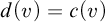


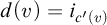

Let
$u,v\in G'$
 be given such that
$u,v$
be given such that
$u,v$
 are adjacent. If both
$u,v\in G$
are adjacent. If both
$u,v\in G$
 , then
$d(u)=c(u)$
, then
$d(u)=c(u)$
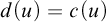 and
$d(v)=c(v)$
and
$d(v)=c(v)$
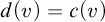 and thus
$d(u)\neq d(v)$
and thus
$d(u)\neq d(v)$
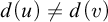 as c is a coloring of G. If both
$u,v\in G'\setminus G$
as c is a coloring of G. If both
$u,v\in G'\setminus G$
 , then there exists some
$U_{i}$
, then there exists some
$U_{i}$
 such that
$u,v\in U_{i}$
such that
$u,v\in U_{i}$
 . This is because
$D'\supseteq D$
. This is because
$D'\supseteq D$
 , meaning that the embedding of the edge connecting
$u,v$
, meaning that the embedding of the edge connecting
$u,v$
 cannot intersect with any part of D. Then
$d(u)=i_{c'(u)}$
cannot intersect with any part of D. Then
$d(u)=i_{c'(u)}$
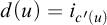 and
$d(v)=i_{c'(v)}$
and
$d(v)=i_{c'(v)}$
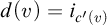 where
$i_{0},i_{1},i_{2},i_{3}$
where
$i_{0},i_{1},i_{2},i_{3}$
 are the four colors unused by c to color
$\partial U_{i}$
are the four colors unused by c to color
$\partial U_{i}$
 . Since
$c'$
. Since
$c'$
 is a coloring of
$G'\setminus G$
is a coloring of
$G'\setminus G$
 , then
$d(u)\neq d(v)$
, then
$d(u)\neq d(v)$
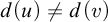 . Finally, consider the case that
$u\in G$
. Finally, consider the case that
$u\in G$
 and
$v\in G'\setminus G$
and
$v\in G'\setminus G$
 . Once again, since
$D'$
. Once again, since
$D'$
 is a plane diagram of
$G'$
is a plane diagram of
$G'$
 , it must be that there exists some
$U_{i}$
, it must be that there exists some
$U_{i}$
 such that
$v\in U_{i}$
such that
$v\in U_{i}$
 and
$u\in \partial U_{i}$
and
$u\in \partial U_{i}$
 , otherwise the embedding of the edge connecting
$u,v$
, otherwise the embedding of the edge connecting
$u,v$
 must intersect D. In such a case,
$d(u)=c(u)$
must intersect D. In such a case,
$d(u)=c(u)$
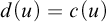 and
$d(v)=i_{c'(v)}$
and
$d(v)=i_{c'(v)}$
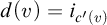 , where
$i_{0},i_{1},i_{2},i_{3}$
, where
$i_{0},i_{1},i_{2},i_{3}$
 are all different from
$c(u)$
are all different from
$c(u)$
 . Therefore,
$d(u)\neq d(v)$
. Therefore,
$d(u)\neq d(v)$
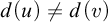 . Thus d is a
$(3(k+1)+1)$
. Thus d is a
$(3(k+1)+1)$
 -coloring of
$G'$
-coloring of
$G'$
 .
.
Now we prove that d is a good coloring of
$D'$
 . The idea is as follows. We shall first show that d is a good coloring of
$D\cup D"$
. The idea is as follows. We shall first show that d is a good coloring of
$D\cup D"$
 . This diagram
$D\cup D"$
. This diagram
$D\cup D"$
 is a plane drawing of the disjoint union of the graph G and the induced subgraph
$G'\setminus G$
is a plane drawing of the disjoint union of the graph G and the induced subgraph
$G'\setminus G$
 . In other words, the edges between the vertices in
$G'\setminus G$
. In other words, the edges between the vertices in
$G'\setminus G$
 and the vertices in G are not shown in the diagram
$D\cup D"$
and the vertices in G are not shown in the diagram
$D\cup D"$
 . However, the intuition is that it is ‘easier’ for some fixed coloring to be good when there are more edges; if d is a good coloring of
$D\cup D"$
. However, the intuition is that it is ‘easier’ for some fixed coloring to be good when there are more edges; if d is a good coloring of
$D\cup D"$
 , then it must also be a good coloring of
$D'$
, then it must also be a good coloring of
$D'$
 . We provide the details below.
Using Fact 3.8, let
${\mathbb {R}}^{2}\setminus D=\bigsqcup _{i\leq m}U_{i}$
 and
${\mathbb {R}}^{2}\setminus D"=\bigsqcup _{j\leq m"}U_{j}"$
and
${\mathbb {R}}^{2}\setminus D"=\bigsqcup _{j\leq m"}U_{j}"$
 . Fix some
$V_{l}$
. Fix some
$V_{l}$
 , an open connected region of
${\mathbb {R}}^{2}\setminus (D\cup D")$
, an open connected region of
${\mathbb {R}}^{2}\setminus (D\cup D")$
 . It is evident that there exists unique
$i,j$
. It is evident that there exists unique
$i,j$
 , such that
$V_{l}\subseteq U_{i}$
, such that
$V_{l}\subseteq U_{i}$
 and
$V_{l}\subseteq U_{j}"$
and
$V_{l}\subseteq U_{j}"$
 . We show now that
$\partial V_{l}\subseteq \partial U_{i}\cup \partial U_{j}"$
. We show now that
$\partial V_{l}\subseteq \partial U_{i}\cup \partial U_{j}"$
 . Let
$x\in \partial V_{l}$
. Let
$x\in \partial V_{l}$
 be given. That is, x is a limit point of
$V_{l}$
be given. That is, x is a limit point of
$V_{l}$
 , and therefore is also a limit point of
$U_{i}$
, and therefore is also a limit point of
$U_{i}$
 . In other words,
$x\in U_{i}$
. In other words,
$x\in U_{i}$
 or
$x\in \partial U_{i}$
or
$x\in \partial U_{i}$
 . By repeating the same argument with
$U_{j}"$
. By repeating the same argument with
$U_{j}"$
 , we also obtain that
$x\in U_{j}"$
, we also obtain that
$x\in U_{j}"$
 or
$x\in \partial U_{j}"$
or
$x\in \partial U_{j}"$
 . Applying the fact that
$\partial V_{l}\subseteq D\cup D"$
. Applying the fact that
$\partial V_{l}\subseteq D\cup D"$
 , we thus obtain that
$x\in \partial U_{i}\cup \partial U_{j}"$
, we thus obtain that
$x\in \partial U_{i}\cup \partial U_{j}"$
 . In addition, since
$x\in \partial U_{i}$
. In addition, since
$x\in \partial U_{i}$
 or
$x\in U_{i}$
or
$x\in U_{i}$
 for each
$x\in \partial V_{l}$
for each
$x\in \partial V_{l}$
 , and
$D\cap D"=\emptyset $
, and
$D\cap D"=\emptyset $
 , we also have that
$\partial V_{l}\cap D"\subseteq U_{i}$
, we also have that
$\partial V_{l}\cap D"\subseteq U_{i}$
 .
.
Partition the vertices in
$\partial V_{l}$
 into those contained in G and those contained in
$G'\setminus G$
into those contained in G and those contained in
$G'\setminus G$
 . Since
$d\restriction G=c$
. Since
$d\restriction G=c$
 is a good
$(3k+1)$
is a good
$(3k+1)$
 -coloring and
$\partial V_{l}\cap D\subseteq \partial U_{i}$
-coloring and
$\partial V_{l}\cap D\subseteq \partial U_{i}$
 , we have that all vertices in
$\partial V_{l}$
, we have that all vertices in
$\partial V_{l}$
 from G are colored with at most
$3k$
from G are colored with at most
$3k$
 colors. Now consider the vertices in
$\partial V_{l}\cap D"$
colors. Now consider the vertices in
$\partial V_{l}\cap D"$
 . We know that all such vertices v are contained within
$U_{i}$
. We know that all such vertices v are contained within
$U_{i}$
 and thus,
$d(v)=i_{c'(v)}$
and thus,
$d(v)=i_{c'(v)}$
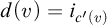 where
$i_{0},i_{1},i_{2},i_{3}$
where
$i_{0},i_{1},i_{2},i_{3}$
 are the four colors unused by c in the coloring of
$\partial U_{i}$
are the four colors unused by c in the coloring of
$\partial U_{i}$
 , and
$c'$
, and
$c'$
 is a good
$4$
is a good
$4$
 -coloring of
$D"$
-coloring of
$D"$
 . Since
$c'$
. Since
$c'$
 is a good
$4$
is a good
$4$
 -coloring of
$D"$
-coloring of
$D"$
 , then it uses at most three colors to color the vertices on
$\partial U_{j}"$
, then it uses at most three colors to color the vertices on
$\partial U_{j}"$
 , say
$0,1,2$
, say
$0,1,2$
 . As a result, d colors the vertices in
$\partial V_{l}\cap D"\subseteq \partial U_{j}"\cap U_{i}$
. As a result, d colors the vertices in
$\partial V_{l}\cap D"\subseteq \partial U_{j}"\cap U_{i}$
 using only the colors
$i_{0},i_{1},i_{2}$
using only the colors
$i_{0},i_{1},i_{2}$
 . Therefore, d uses at most
$3k+3$
. Therefore, d uses at most
$3k+3$
 colors to color the vertices in
$\partial V_{l}$
colors to color the vertices in
$\partial V_{l}$
 and is thus a good
$(3(k+1)+1)$
and is thus a good
$(3(k+1)+1)$
 -coloring of
$D\cup D"$
-coloring of
$D\cup D"$
 . Finally, to see that d is a good
$(3(k+1)+1)$
. Finally, to see that d is a good
$(3(k+1)+1)$
 -coloring of
$D'$
-coloring of
$D'$
 , recall that
$D\cup D"$
, recall that
$D\cup D"$
 is the drawing of
$G'$
is the drawing of
$G'$
 without the edges between vertices in
$G'\setminus G$
without the edges between vertices in
$G'\setminus G$
 and G. In other words, for every connected open region of
${\mathbb {R}}^{2}\setminus D'$
and G. In other words, for every connected open region of
${\mathbb {R}}^{2}\setminus D'$
 , there is a connected open region of
${\mathbb {R}}^{2}\setminus (D\cup D")$
, there is a connected open region of
${\mathbb {R}}^{2}\setminus (D\cup D")$
 such that every vertex in the boundary of the former is contained in the boundary of the latter. It follows immediately that d is a good
$(3(k+1)+1)$
such that every vertex in the boundary of the former is contained in the boundary of the latter. It follows immediately that d is a good
$(3(k+1)+1)$
 -coloring of
$D'$
-coloring of
$D'$
 .
.
Lemma 3.12. Let G be a finite planar graph with plane diagram D. Let
$G'\supseteq G$
 be a countable planar graph with some plane diagram
$D'\supseteq D$
be a countable planar graph with some plane diagram
$D'\supseteq D$
 . If D has a good
$(3k+1)$
. If D has a good
$(3k+1)$
 -coloring c, then c can be extended to a
$(3(k+1)+1)$
-coloring c, then c can be extended to a
$(3(k+1)+1)$
 -coloring of
$G'$
-coloring of
$G'$
 .
.
Proof. We apply a standard compactness argument. Let a finite planar graph G with plane diagram D be given. Also let
$\sigma $
 be a good
$(3k+1)$
be a good
$(3k+1)$
 -coloring of D. Consider the tree T defined as follows:
-
• $\langle \sigma ,G,D\rangle \in T$
. -
• If $\langle \xi ,H,P\rangle \in T$
, then
$\langle \tau ,H',P'\rangle \in T$
provided that all of the following holds.
$H'\subseteq G'$
and
$P'\subseteq D'$
.
$\tau \supseteq \xi $
is a good
$(3(k+1)+1)$
-coloring of
$P'\supseteq P$
.
$P'$
is a plane diagram of
$H'$
. And
$H'$
extends H by exactly one vertex.








Considering the (restricted) plane diagrams up to equivalence (recall Definition 1.5), it is clear that T is finitely branching. To see that it is infinite, since
$G'$
 is an infinite graph with diagram
$D'$
is an infinite graph with diagram
$D'$
 , then it remains to argue that there always exists some
$(3(k+1)+1)$
, then it remains to argue that there always exists some
$(3(k+1)+1)$
 -coloring
$\tau $
-coloring
$\tau $
 of
$D'\restriction H$
of
$D'\restriction H$
 for each finite induced subgraph H where
$G\subseteq H\subseteq G'$
for each finite induced subgraph H where
$G\subseteq H\subseteq G'$
 . Since
$H\supseteq G$
. Since
$H\supseteq G$
 is a finite planar graph with a plane diagram
$D'\restriction H\supseteq D$
is a finite planar graph with a plane diagram
$D'\restriction H\supseteq D$
 , then applying Lemma 3.11 allows us to conclude that there is some good
$(3(k+1)+1)$
, then applying Lemma 3.11 allows us to conclude that there is some good
$(3(k+1)+1)$
 -coloring
$\tau \supseteq \sigma $
-coloring
$\tau \supseteq \sigma $
 . Thus there must be a path through T and the first coordinate of this path provides a
$(3(k+1)+1)$
. Thus there must be a path through T and the first coordinate of this path provides a
$(3(k+1)+1)$
 -coloring of
$G'$
-coloring of
$G'$
 .
.
Applying Lemmas 3.1 3.6 and 3.12, we can now complete the picture illustrated in Figure 5 and also compare the Weihrauch degrees of the different coloring principles.
Theorem 3.13.
${\mathtt {DNR}}{\not \!\!{\leq _{\mathsf {W}}}}{\mathtt {ConnCOL}}(7)$
 and
${\mathtt {DNR}}{\not \!\!{\leq _{\mathsf {W}}}}{\mathtt {COL}}^{*}(7)$
and
${\mathtt {DNR}}{\not \!\!{\leq _{\mathsf {W}}}}{\mathtt {COL}}^{*}(7)$
 .
.
Proof. We adopt a similar idea as in the proof of Theorem 3.2. Roughly speaking, Lemmas 3.6 and 3.12 allow us to extend
$4$
 -colorings into
$7$
-colorings into
$7$
 -colorings. We will present the proof for
${\mathtt {DNR}}{\leq _{\mathsf {W}}} {\mathtt {COL}}^{*}(7)$
-colorings. We will present the proof for
${\mathtt {DNR}}{\leq _{\mathsf {W}}} {\mathtt {COL}}^{*}(7)$
 as it has some slight intricacies not required for
${\mathtt {DNR}}{\leq _{\mathsf {W}}} {\mathtt {ConnCOL}}(7)$
as it has some slight intricacies not required for
${\mathtt {DNR}}{\leq _{\mathsf {W}}} {\mathtt {ConnCOL}}(7)$
 , but essentially the same proof can be used to show the latter.
Suppose to the contrary that
${\mathtt {DNR}}{\leq _{\mathsf {W}}} {\mathtt {COL}}^{*}(7)$
 . Then, there are Turing reductions
$\Phi ,\Psi $
. Then, there are Turing reductions
$\Phi ,\Psi $
 such that
$\Phi (f)$
such that
$\Phi (f)$
 produces a planar graph with a plane diagram D given any oracle f. And given any
$7$
produces a planar graph with a plane diagram D given any oracle f. And given any
$7$
 -coloring h of G,
$\Psi (h\oplus f)$
-coloring h of G,
$\Psi (h\oplus f)$
 satisfies
${\mathtt {DNR}}$
satisfies
${\mathtt {DNR}}$
 .
.
Let f be the empty oracle;
$f_{s}=0^{s}$
 for each
$s\in \omega $
for each
$s\in \omega $
 . Define
$\psi ^{f}(x)=\Psi (h\oplus f)(x)$
. Define
$\psi ^{f}(x)=\Psi (h\oplus f)(x)$
 in a similar way as in the proof of Theorem 3.2. At each stage s, compute the graph and diagram
$G_{s},D_{s}$
in a similar way as in the proof of Theorem 3.2. At each stage s, compute the graph and diagram
$G_{s},D_{s}$
 given by
$\Phi (f_{s})$
given by
$\Phi (f_{s})$
 . Instead of directly searching for a coloring of
$G_{s}$
. Instead of directly searching for a coloring of
$G_{s}$
 , we adopt the idea presented in Lemma 3.10 and search instead for a
$4$
, we adopt the idea presented in Lemma 3.10 and search instead for a
$4$
 -coloring of an extended graph
$G_{s}'\supseteq G_{s}$
-coloring of an extended graph
$G_{s}'\supseteq G_{s}$
 which enumerates a new vertex for each open connected component of
${\mathbb {R}}^{2}\setminus D_{s}$
which enumerates a new vertex for each open connected component of
${\mathbb {R}}^{2}\setminus D_{s}$
 and connects the vertex to all vertices on the boundary of the open connected component. As explained in the lemma,
$G_{s}'$
and connects the vertex to all vertices on the boundary of the open connected component. As explained in the lemma,
$G_{s}'$
 is planar and must thus have some
$4$
is planar and must thus have some
$4$
 -coloring
$h_{s}$
-coloring
$h_{s}$
 . Furthermore,
$h_{s}\restriction G_{s}$
. Furthermore,
$h_{s}\restriction G_{s}$
 is a good
$4$
is a good
$4$
 -coloring of
$D_{s}$
-coloring of
$D_{s}$
 . There must thus exist some stage s such that
$\Psi (h_{s}\restriction G_{s}\oplus f_{s})(x)[s]{\downarrow }$
. There must thus exist some stage s such that
$\Psi (h_{s}\restriction G_{s}\oplus f_{s})(x)[s]{\downarrow }$
 , otherwise by a compactness argument, there is some h a
$4$
, otherwise by a compactness argument, there is some h a
$4$
 -coloring of
$\Phi (f)$
-coloring of
$\Phi (f)$
 such that
$\Psi (h\oplus f)(x){\uparrow }$
such that
$\Psi (h\oplus f)(x){\uparrow }$
 . By the recursion theorem, there exists x such that
$\varphi _{x}^{f}(x)=\psi ^{f}(x)$
. By the recursion theorem, there exists x such that
$\varphi _{x}^{f}(x)=\psi ^{f}(x)$
 . We thus have that for some s and some
$4$
. We thus have that for some s and some
$4$
 -coloring
$h_{s}$
-coloring
$h_{s}$
 of
$G_{s}'\supseteq \Phi (f_{s})$
of
$G_{s}'\supseteq \Phi (f_{s})$
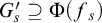 ,
,

Furthermore,
$h_{s}\restriction G_{s}$
 is a good
$4$
is a good
$4$
 -coloring of
$D_{s}$
-coloring of
$D_{s}$
 . Now applying Lemma 3.12 allows us to conclude that for any planar extension G of
$G_{s}$
. Now applying Lemma 3.12 allows us to conclude that for any planar extension G of
$G_{s}$
 , there is some h a
$7$
, there is some h a
$7$
 -coloring of G which extends
$h_{s}\restriction G_{s}$
-coloring of G which extends
$h_{s}\restriction G_{s}$
 . In particular,

A contradiction to the assumption that
$\Phi ,\Psi $
 witnesses
${\mathtt {DNR}}{\leq _{\mathsf {W}}} {\mathtt {COL}}^{*}(7)$
witnesses
${\mathtt {DNR}}{\leq _{\mathsf {W}}} {\mathtt {COL}}^{*}(7)$
 .
.
Theorem 3.14. For any
$n>0$
 and for any
$i<4$
and for any
$i<4$
 ,
,
-
• ${\mathtt {COL}}(4n+i){\not \!\!{\leq _{\mathsf {W}}}}{\mathtt {ConnCOL}}(3(n+1)+1)$
, and -
• ${\mathtt {COL}}(4n+i){\not \!\!{\leq _{\mathsf {W}}}}{\mathtt {COL}}^{*}(3(n+1)+1)$
.


Proof. We follow the idea presented in the proof of Theorem 3.3. Once again, we will only present the proof for the slightly more complicated
${\mathtt {COL}}^{*}$
 . Suppose to the contrary that
${\mathtt {COL}}(4n+i){\leq _{\mathsf {W}}} {\mathtt {COL}}^{*}(3(n+1)+1)$
. Suppose to the contrary that
${\mathtt {COL}}(4n+i){\leq _{\mathsf {W}}} {\mathtt {COL}}^{*}(3(n+1)+1)$
 . That is, there exists
$\Phi ,\Psi $
. That is, there exists
$\Phi ,\Psi $
 , Turing reductions such that
$\Phi (G)$
, Turing reductions such that
$\Phi (G)$
 produces a countable planar graph H with a diagram D and given any
$(3(n+1)+1)$
produces a countable planar graph H with a diagram D and given any
$(3(n+1)+1)$
 -coloring h of H,
$\Psi (h\oplus G)$
-coloring h of H,
$\Psi (h\oplus G)$
 is a
$(4n+i)$
is a
$(4n+i)$
 -coloring of G. Start by enumerating sufficiently many
$K_{4}$
-coloring of G. Start by enumerating sufficiently many
$K_{4}$
 graphs to construct a
$W_{m}$
graphs to construct a
$W_{m}$
 (recall the proof of Theorem 2.7) where m is the least such that
$m\geq \lceil (4n+i)/4)\rceil $
(recall the proof of Theorem 2.7) where m is the least such that
$m\geq \lceil (4n+i)/4)\rceil $
 .
.
Using the same procedure as described in the proof of Theorem 3.3 to define h, a coloring of H and build
$W_{m}^{g}$
 (recall Notation 2.9) where
$g=\Psi (h\oplus G)$
(recall Notation 2.9) where
$g=\Psi (h\oplus G)$
 . The only difference is that each time we extend
$h_{l}$
. The only difference is that each time we extend
$h_{l}$
 to
$h_{l+1}$
to
$h_{l+1}$
 for
$l<m-1$
for
$l<m-1$
 , we use Lemma 3.11 in place of Lemma 3.1. That is, for each
$l<m$
, we use Lemma 3.11 in place of Lemma 3.1. That is, for each
$l<m$
 ,
$h_{l}$
,
$h_{l}$
 is a good
$(3l+1)$
is a good
$(3l+1)$
 -coloring of some finite restriction of H. Finally, we use Lemma 3.12 to extend
$h_{m-1}$
-coloring of some finite restriction of H. Finally, we use Lemma 3.12 to extend
$h_{m-1}$
 to h a
$(3m+1)$
to h a
$(3m+1)$
 -coloring of H. Since
$m\leq n+1$
-coloring of H. Since
$m\leq n+1$
 , h is a
$(3(n+1)+1)$
, h is a
$(3(n+1)+1)$
 -coloring of H but H contains a
$W_{m}^{\Psi (h\oplus G)}$
-coloring of H but H contains a
$W_{m}^{\Psi (h\oplus G)}$
 and thus cannot be
$(4n+i)$
and thus cannot be
$(4n+i)$
 -colored by
$\Psi (h\oplus G)$
-colored by
$\Psi (h\oplus G)$
 .
.
From the theorem, we have the following interesting result.
Corollary 3.15. For all
$n\geq 16$
 ,
,
-
• ${\mathtt {ConnCOL}}(n)<_{W}{\mathtt {COL}}(n)$
, and -
• ${\mathtt {COL}}^{*}(n)<_{W}{\mathtt {COL}}(n)$
.


4 Further questions
We have shown that for each n, the principles
${\mathtt {COL}}(n),{\mathtt {ConnCOL}}(n),$
 and
${\mathtt {COL}}^{*}(n)$
and
${\mathtt {COL}}^{*}(n)$
 are equivalent to
${{\mathtt {WKL}}}$
are equivalent to
${{\mathtt {WKL}}}$
 over
${\mathtt {RCA}_{0}}$
over
${\mathtt {RCA}_{0}}$
 . However, for the cases of
$n>4$
. However, for the cases of
$n>4$
 , non-uniform proofs were used to obtain the reversals. We also showed that this non-uniformity is necessary for
$n\geq 7$
, non-uniform proofs were used to obtain the reversals. We also showed that this non-uniformity is necessary for
$n\geq 7$
 but leave the cases for
$n=5,6$
but leave the cases for
$n=5,6$
 open. A possible way to tackle this question is to consider the uniformity of reductions between the coloring principles. It is trivial to see that
${\mathtt {COL}}(7){\leq _{\mathsf {sW}}}{\mathtt {COL}}(6){\leq _{\mathsf {sW}}}{\mathtt {COL}}(5){\leq _{\mathsf {sW}}}{\mathtt {COL}}(4)$
open. A possible way to tackle this question is to consider the uniformity of reductions between the coloring principles. It is trivial to see that
${\mathtt {COL}}(7){\leq _{\mathsf {sW}}}{\mathtt {COL}}(6){\leq _{\mathsf {sW}}}{\mathtt {COL}}(5){\leq _{\mathsf {sW}}}{\mathtt {COL}}(4)$
 . But it is still unknown which of the reductions (other than
${\mathtt {COL}}(4){\not \!\!{\leq _{\mathsf {W}}}}{\mathtt {COL}}(7)$
. But it is still unknown which of the reductions (other than
${\mathtt {COL}}(4){\not \!\!{\leq _{\mathsf {W}}}}{\mathtt {COL}}(7)$
 ) can be made strict. Similarly, we leave open the question of whether or not the implications presented in Figure 5 can be made strict. More generally, we also do not know if
${\mathtt {COL}}(4n+i)$
) can be made strict. Similarly, we leave open the question of whether or not the implications presented in Figure 5 can be made strict. More generally, we also do not know if
${\mathtt {COL}}(4n+i)$
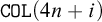 collapses to
${\mathtt {COL}}(4n)$
collapses to
${\mathtt {COL}}(4n)$
 . Similar questions for
${\mathtt {ConnCOL}}$
. Similar questions for
${\mathtt {ConnCOL}}$
 and
${\mathtt {COL}}^{*}$
and
${\mathtt {COL}}^{*}$
 also seem to be interesting.
Further analysis by comparing these principles against other benchmark principles in the Weihrauch degrees could also be performed. For instance,
$\mathtt {LLPO}$
 and
$\mathtt {K}_{{\mathbb {N}}}$
and
$\mathtt {K}_{{\mathbb {N}}}$
 are both known to be below
${{\mathtt {WKL}}}$
are both known to be below
${{\mathtt {WKL}}}$
 in the Weihrauch setting. However, the gadgets used in this article do not seem to lend itself well to investigating the relations between such principles and the various coloring principles. Other Weihrauch theoretic properties of the colouring principles could also be studied: we note that each of the principles
${\mathtt {COL}}(n),{\mathtt {ConnCOL}}(n)$
in the Weihrauch setting. However, the gadgets used in this article do not seem to lend itself well to investigating the relations between such principles and the various coloring principles. Other Weihrauch theoretic properties of the colouring principles could also be studied: we note that each of the principles
${\mathtt {COL}}(n),{\mathtt {ConnCOL}}(n)$
 , and
${\mathtt {COL}}^{*}(n)$
, and
${\mathtt {COL}}^{*}(n)$
 are all parallelizable but we do not know if they are cylinders (see [Reference Brattka and Gherardi2] for definitions). Returning to the reverse math setting, investigations of the principle “Every planar graph has some n-coloring.” could also be interesting. It is clearly provable in
${{\mathtt {WKL}}}_{0}$
are all parallelizable but we do not know if they are cylinders (see [Reference Brattka and Gherardi2] for definitions). Returning to the reverse math setting, investigations of the principle “Every planar graph has some n-coloring.” could also be interesting. It is clearly provable in
${{\mathtt {WKL}}}_{0}$
 , and applying [Reference Bean1, Theorem 2] gives that it does not hold in
${\mathtt {RCA}_{0}}$
, and applying [Reference Bean1, Theorem 2] gives that it does not hold in
${\mathtt {RCA}_{0}}$
 . However whether it is equivalent to
${{\mathtt {WKL}}}$
. However whether it is equivalent to
${{\mathtt {WKL}}}$
 seems to still be open and a similar Weihrauch analysis of this principle could also be carried out.
Funding
K.M.N. was supported by the Ministry of Education, Singapore, under its Academic Research Fund Tier 2 (MOE-T2EP20222-0018) and Academic Research Fund Tier 1 (RG104/24).


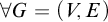






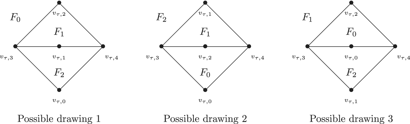
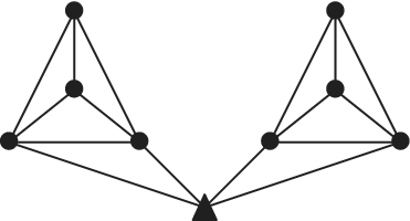

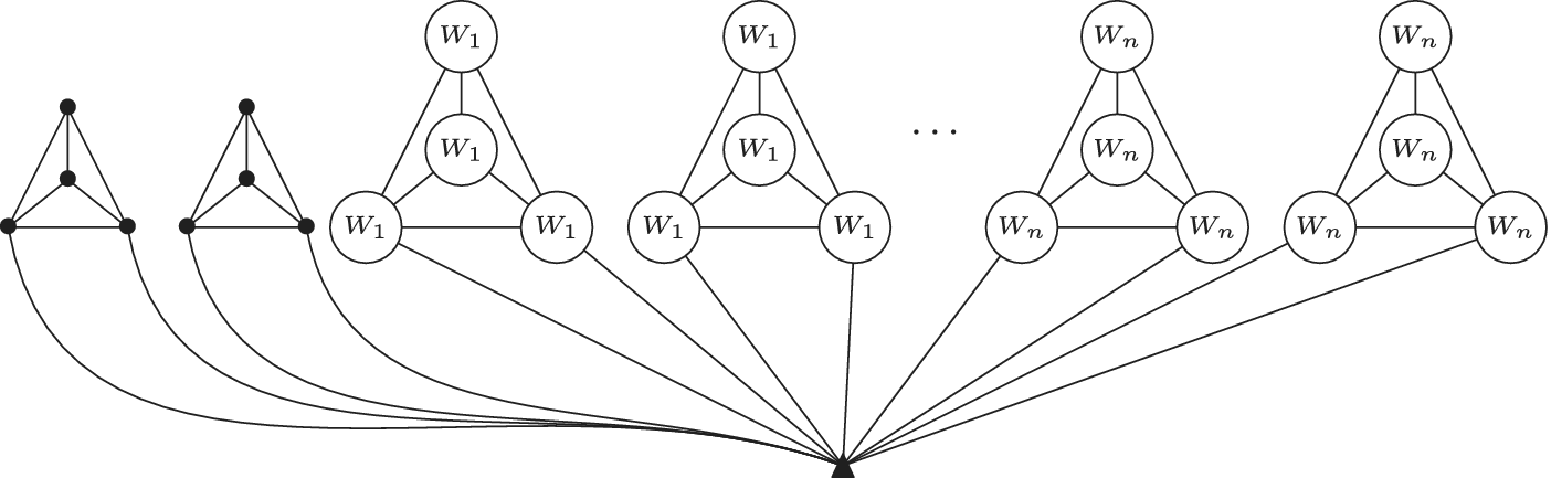

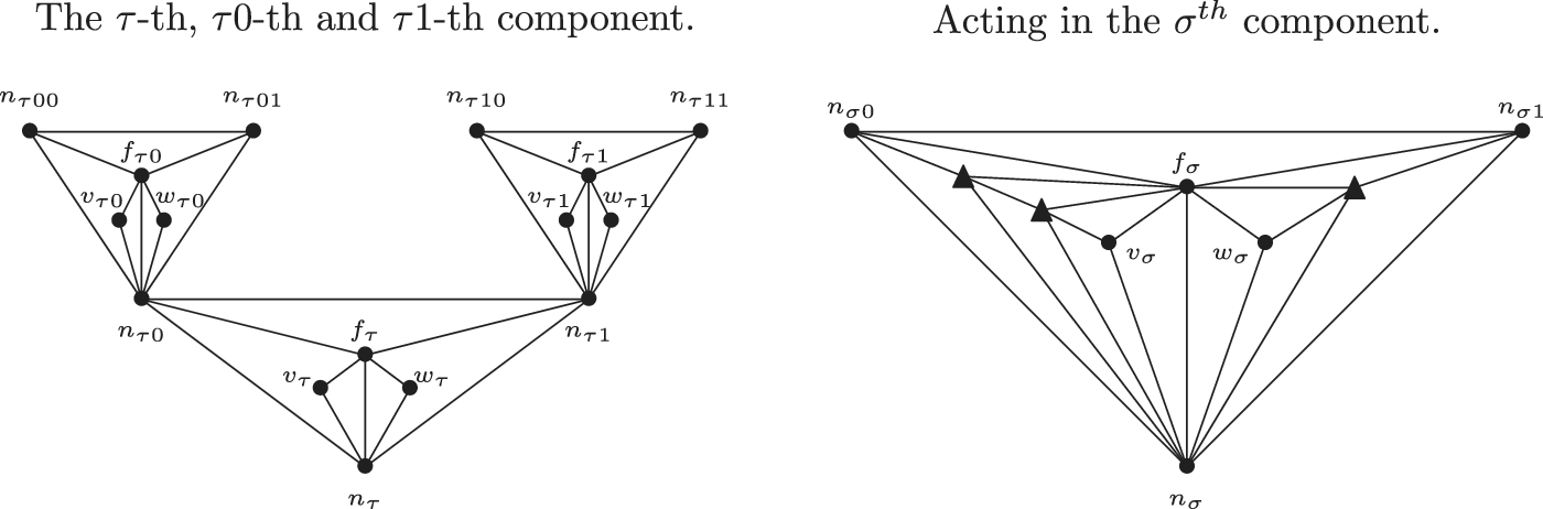


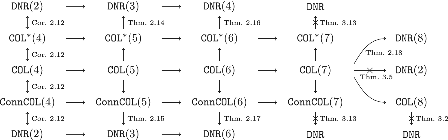


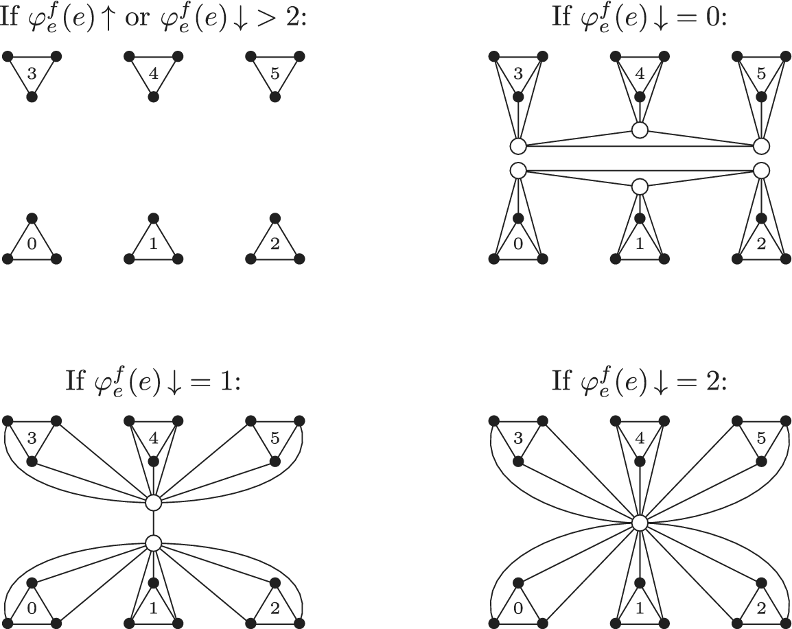
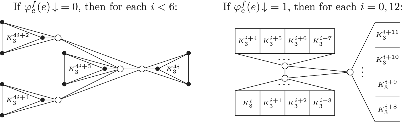

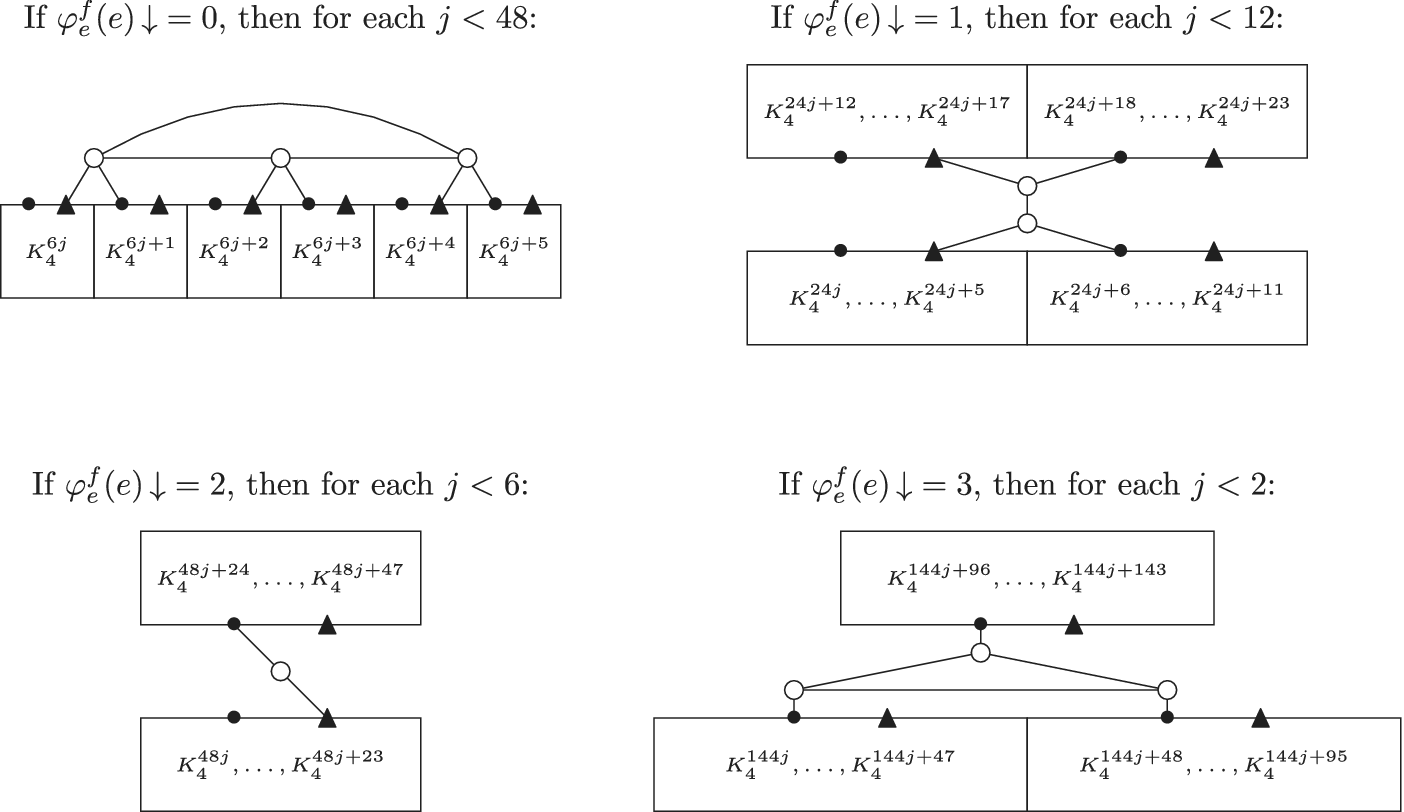


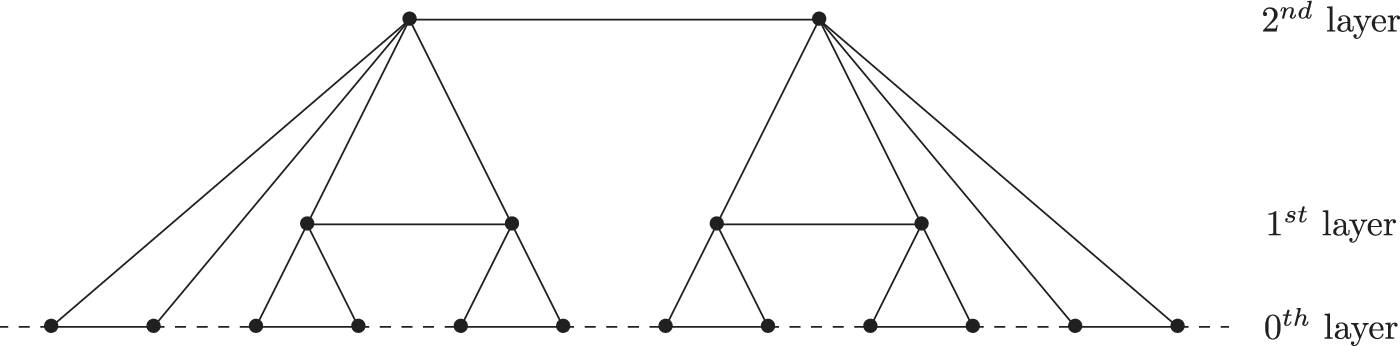


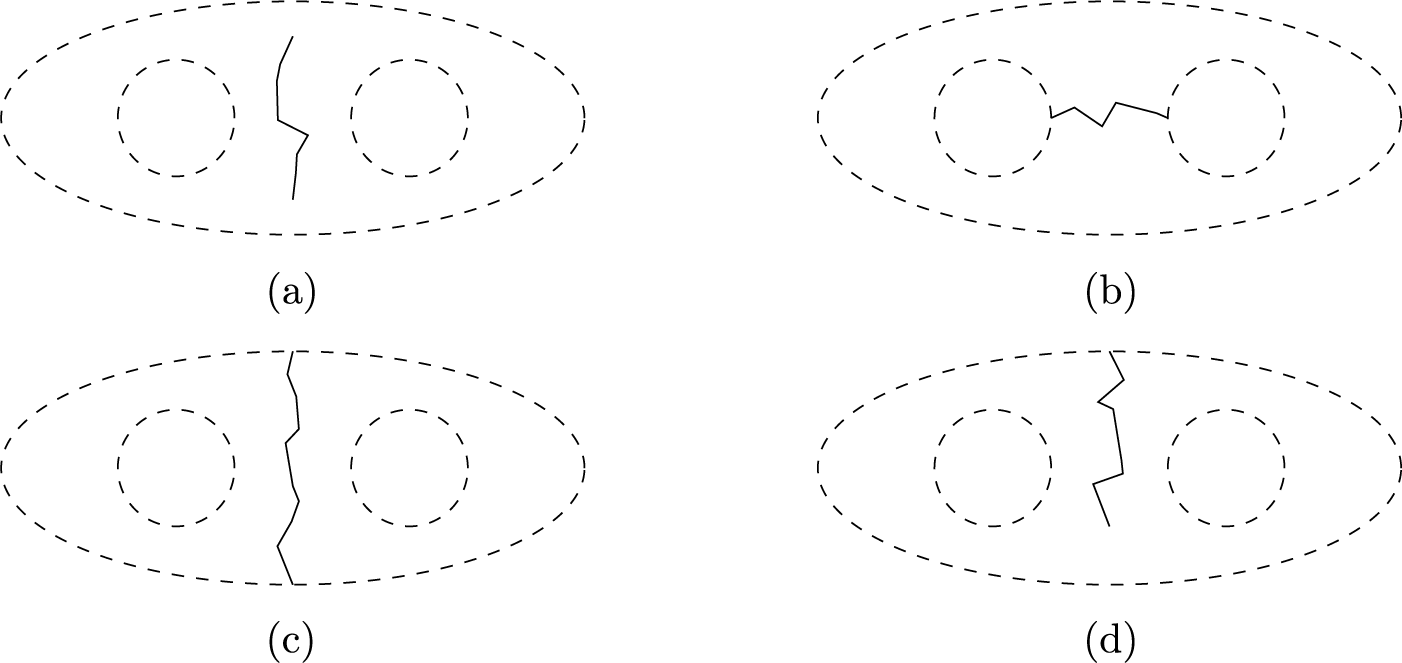

 Open access

