


1. Introduction
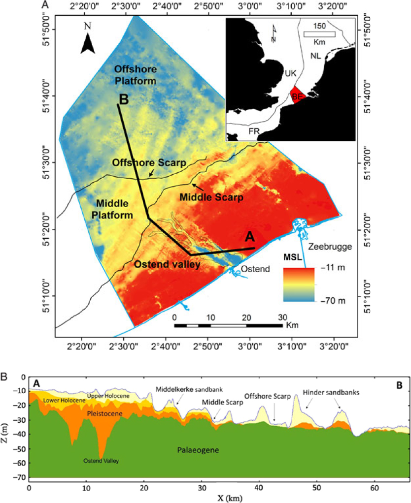
The Belgian Continental Shelf (BCS) is bounded in the north and south by the Dutch and French parts of the North Sea, on the west by the British part and on the east by the Belgian coast (Fig. 1). The BCS is a sediment-depleted shallow shelf environment comprising a series of sandbanks. There is no distinct shelf break (De Batist, Reference De Batist1989), so there is very little accommodation space to accumulate younger and preserve older sediments. In turn this caused important recycling and redistribution of the sediment, creating a complex thin and discontinuous Quaternary sediment cover.
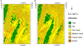
(A) Map showing the depth of the Top-Palaeogene unconformity and the main geomorphological features: the Middle and Offshore Platform, separated by the Middle and Offshore scarp (De Clercq et al., Reference De Clercq, Chademenos, Van Lancker and Missiaen2016). These scarps were used to split up the model into regions with similar lithological characteristics. (B) Cross-section showing the extent and geometry of each stratigraphical unit subdividing the Cainozoic sediments of the BCS. Most of the sandbanks (e.g. Middelkerke, Hinder) have a characteristic internal architecture.
There is a high demand to exploit the resources within this sedimentary cover (Van Lancker et al., Reference Van Lancker, Bonne, Garel, Degrendele, Roche, Van den Eynde, Bellec, Brière, Collins, Velegrakis, Van Lancker, Bonne, Uriarte and Collins2010) and the demand is only increasing due to coastal nourishment projects and new visions for the development of the marine and coastal zone of Belgium. Availability of sand is critical to support these initiatives, and therefore the research project TILES was initiated to develop Transnational and Integrated Long-term Marine Exploitation Strategies (Van Lancker et al., Reference Van Lancker, Francken, Kint, Terseleer, Van den Eynde, De Mol, De Tré, De Mol, Missiaen, Hademenos, Bakker, Busschers, Maljers, Stafleu, Van Heteren, Diviacco, Leadbetter and Glaves2017). Hitherto, no quantitative resource data were available, and also internationally such data remain scarce, apart from site-related datasets. In a marine aggregate context, it is also important to have information on admixtures that may adversely affect the quality of the resource (e.g. shells, mud and gravel content) and/or the environment (e.g. mud; Newell et al., Reference Newell, Seiderer and Hitchcock1998). Therefore, we opted to develop a three-dimensional (3D) voxel model allowing us to obtain a holistic view on resource quality and quantity of the Quaternary over wide areas and enabling the addition of any desired information relevant from a resource or environmental impact perspective.
For this application, voxels are a regular grid of rectangular blocks with defined dimensions (x, y, z) in a Cartesian coordinate system. Each voxel in the model can contain multiple attributes describing, for example, the stratigraphy, or the spatial variation of lithology in geological units and other parameters such as uncertainty. Because of their structure, voxels can better define complex geology and heterogeneities within geological layers (Stafleu et al., Reference Stafleu, Maljers, Gunnink, Menkovic and Busschers2011). In addition, voxel models can be created using stochastic techniques that allow the construction of multiple, equally probable 3D realisations. Furthermore, they facilitate easy querying and analysis: for example, volume calculations can be performed by selecting and counting the voxels that meet certain criteria.
To model aggregate resources in 3D, it is important to define deposits with uniform lithological properties. In a voxel model, 3D interpolation techniques can be implemented to estimate a representative lithological class (or another property) for each voxel based on the lithological description of boreholes available in the model area (Van Haren et al., Reference Van Haren, Dirix, De Koninck, De Groot and De Nil2016). In many cases, modelling results can be greatly improved by subdividing the 3D volume into lithostratigraphical units that have uniform sediment characteristics. For example, in the GeoTOP voxel model of the onshore part of the Netherlands (Stafleu et al., Reference Stafleu, Maljers, Gunnink, Menkovic and Busschers2011, Reference Stafleu, Maljers, Busschers, Gunnink, Schokker, Dambrink, Hummelman and Schijf2012) the borehole descriptions were first used to construct 2D bounding surfaces. These surfaces represented the top and base of each of the lithostratigraphical units and were used to place each voxel in the model within the correct unit. Next, the 3D interpolation of lithological class was performed for each lithostratigraphical unit separately.
Creating bounding surfaces from borehole data works well if the spatial data density of the boreholes is relatively high, as is the case in the GeoTOP model (~10 boreholes per km2 on average). In the BCS however, borehole density is only about 0.3 per km2. Such low borehole density necessitates the incorporation of other data sources. Most evident are geophysical line data such as shallow 2D/3D seismic profiles that allow the interpretation of ‘horizons’ to subsequently allow the generation of bounding surfaces to define the different lithostratigraphical units in 3D modelling (e.g. Bartakovics et al., Reference Bartakovics, Koma, Székely, Kovács, András Zámolyi and Tímár2013; Van Heteren et al., Reference Van Heteren, Meekes, Bakker, Gaffney, Fitch, Gearey and Paap2014; Jørgensen et al., Reference Jørgensen, Høyer, Sandersen, He and Foged2015).
With the advent of 3D models, their increasing complexity and the variety of methods employed, finding better ways to assess the quality and reliability of the models becomes crucial. Using stochastic models, the probability of occurrences of each lithological class can be calculated as a first estimate of model uncertainty. To summarise the probabilities per voxel, Wellmann & Regenauer-Lieb (Reference Wellmann and Regenauer-Lieb2012) suggested calculating information entropy as a measure of model uncertainty. The quality measure thus obtained can be used to compare different versions of a model.
In this paper, a step-by-step modelling approach is described to depict the quality and quantity of the available geological resources in the BCS. For the first time, 3D stochastic modelling is applied to quantify sand resources in a marine setting making use of both borehole and seismic data. For this application, the approach is also new in the sense that it incorporates various levels of geological knowledge in the modelling process and this is shown to improve the characterisation of the subsurface. A more detailed case study is presented to demonstrate how the resolution of a model affects the depiction of the lithostratigraphy and the volume of the resource.
2. Geology and stratigraphy
2.1. Palaeogene
The BCS is marked by two major geological units greatly varying in lithology and stratigraphy. These units, respectively the Palaeogene and Quaternary, are bounded by the Top-Palaeogene unconformity (De Clercq et al., Reference De Clercq, Chademenos, Van Lancker and Missiaen2016). The Palaeogene is a polygenetic layer composed of compacted clays, sands and sandy clays that were deposited in a shallow-marine to outer-shelf environment (Le Bot et al., Reference Le Bot, Van Lancker, Deleu, De Batist and Henriet2003). The geological units within the Palaeogene range in age from the upper Palaeogene to the upper Eocene. The layers dip towards the NE by approximately 1°. Their lithology varies from west to east, from consolidated clays (Ypresian) to alternating sequences of silt and clay, but also silty sand, muddy sand and even calcareous sandstone beds (Le Bot et al., Reference Le Bot, Van Lancker, Deleu, De Batist, Henriet and Haegeman2005).
The top of the Palaeogene is an angular unconformity (Fig. 1) representing a hiatus in time between the Lower and Middle Eocene formations (De Batist, Reference De Batist1989) and the overlying Quaternary deposits. The depth of the surface varies between 8 and 70 m below lowest astronomical tide (LAT), and its geomorphology is characterised by a series of features ranging from planation surfaces, bounded by scarps and slope breaks, to palaeovalleys and elongated depressions (Liu, Reference Liu1990; Liu et al., Reference Liu, Missiaen and Henriet1992; Mathys, Reference Mathys2009; De Clercq et al., Reference De Clercq, Chademenos, Van Lancker and Missiaen2016).
2.2. Quaternary
Thin, discontinuous/heterogeneous Pleistocene and Holocene sediments overlay the unconformity (Mathys, Reference Mathys2009). The variability of the geological formations of the Quaternary poses a major challenge when modelling; the lithostratigraphy content of each sandbank is unique and interpolation will cause generalisations that may lead to faulty assumptions about their geological content. To avoid this, the stratigraphical layers that will be used must be carefully defined. The Pleistocene sediments occur in two main regions of the BCS. On the Offshore Platform, they form the core of the sandbanks (e.g. Hinder Banks), and closer to the coast they are preserved in palaeovalleys such as the Ostend Valley (Fig. 1) (De Clercq et al., Reference De Clercq, Chademenos, Van Lancker and Missiaen2016, Reference De Clercq, Missiaen, Wallinga, Hurtado, Versendaal, Mathys and De Batist2018). In the Middle Platform region they were mostly eroded down to the Palaeogene clays by both the Eemian and the Holocene transgressions (Mathys, Reference Mathys2009). The Pleistocene sediments originate mainly from the Eemian interglacial period and comprise mixed sediments spanning from gravel to clay. There is a lateral difference in lithology between the nearshore area, where clay to fine sands predominate (in the palaeovalleys), and the offshore area where coarser-grained sands with abundant shells are found.
The Holocene sediments are diverse in origin and composition. They form the major part of the tidal sandbanks of the BCS (e.g. Trentesaux et al., Reference Trentesaux, Stolk and Berne1999; Mathys Reference Mathys2009; Van Lancker et al., Reference Van Lancker, Bonne, Garel, Degrendele, Roche, Van den Eynde, Bellec, Brière, Collins, Velegrakis, Van Lancker, Bonne, Uriarte and Collins2010). Two layers are distinguished, the Lower and Upper Holocene respectively. In the nearshore area, the Lower Holocene layer (LHL) is representative of a tidal flat environment (Mathys, Reference Mathys2009) which was formed around 10,950 cal BP (before present) until it was submerged around 7500 cal BP. This Lower Holocene layer was first defined in the Middelkerke Bank (Fig. 1); its sediments varied from coarse-grained to very-fine sand. The Upper Holocene layer (UHL) covers the total BCS and forms the most important sand resource. In the nearshore area, south of the middle scarp (Fig. 1), it predominantly consists of fine sands related to an estuarine–marine depositional environment. In the offshore area, north of the middle scarp (Fig. 1), the layer comprises coarser material, with medium to coarse sand being typical for the offshore marine depositional environment.
2.3. Methodology
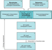
To model offshore aggregate resources, a methodological workflow was developed based on the voxel modelling approach of Stafleu et al. (Reference Stafleu, Maljers, Gunnink, Menkovic and Busschers2011) and expanded with seismic data. It comprises the following steps (Fig. 2):
(1a) Standardisation and lithological classification of borehole descriptions
(1b, 3) Delineation of seismic acoustic facies and their seismostratigraphical interpretation
(2) Stratigraphic interpretation of the boreholes
(4) Construction of the 2D stratigraphical layer model
(5) Assignment of lithostratigraphical units to the 3D voxel model
(6) 3D interpolation of lithological class within each lithostratigraphical unit
(7) Assessment of the information entropy of the model.
Modelling procedure flow chart.
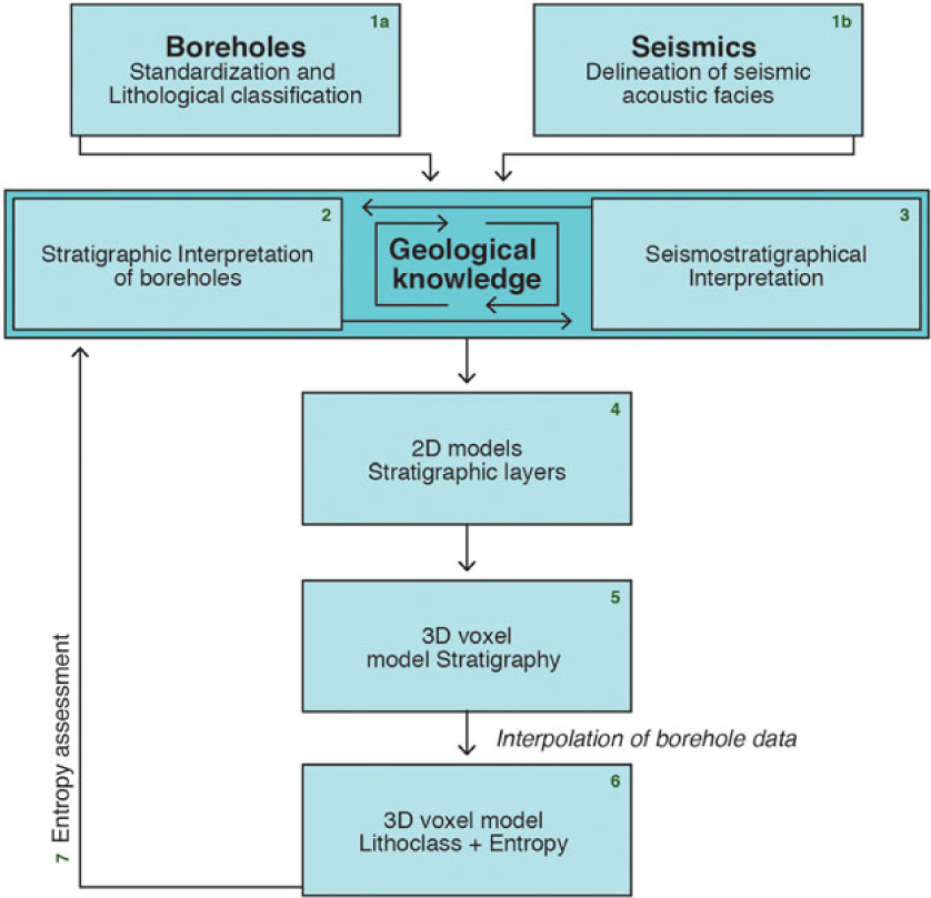
A detailed description of steps 1 to 7, following an iterative process as is indicated in Fig. 2, is given below.
2.4. Step 1a: Standardisation and lithological classification of borehole descriptions
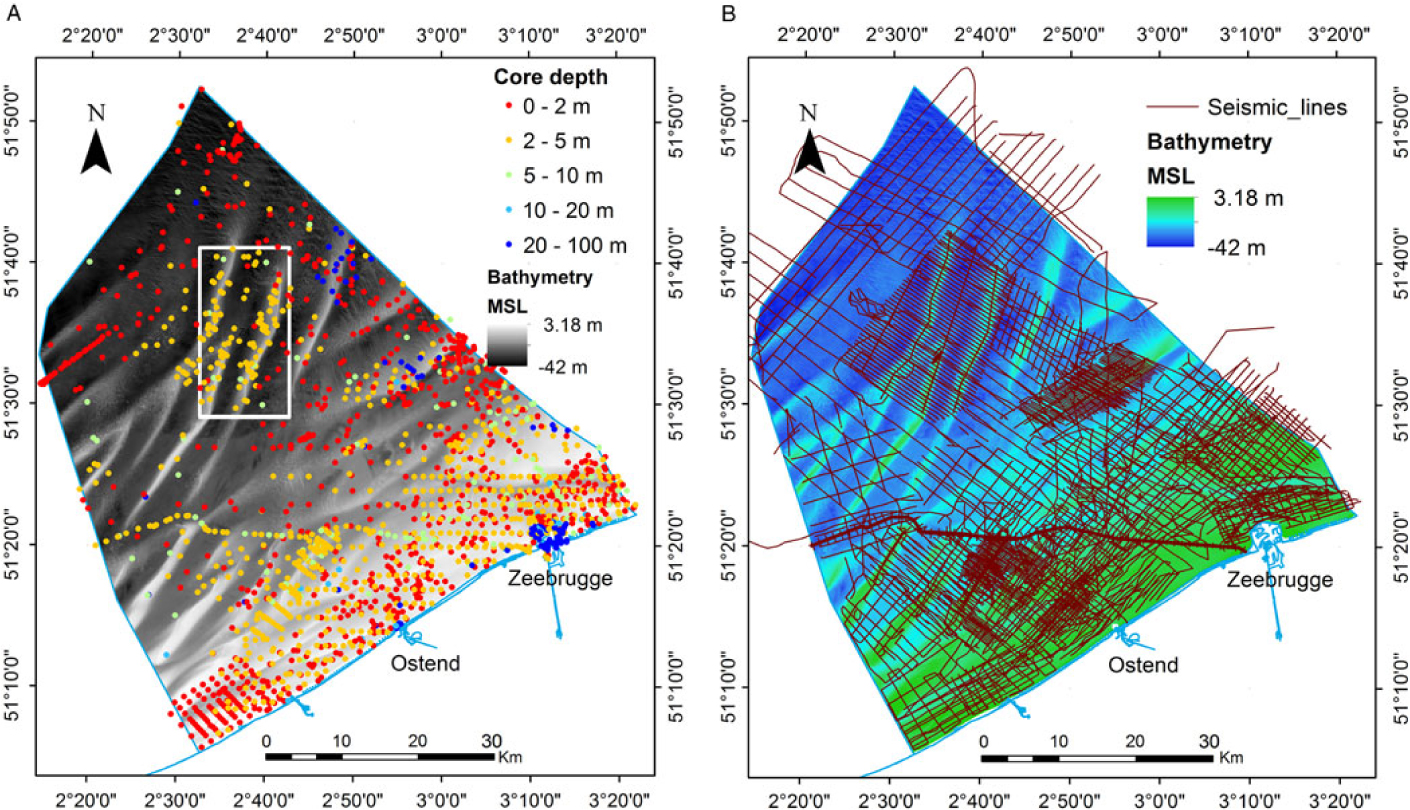
Our core dataset contained a total of 1770 cores on the BCS extending to 1 km beyond the border (Fig. 3A) provided by the Royal Belgian Institute of Natural Sciences (Kint & Van Lancker, Reference Kint and Van Lancker2016). Data originated from the public and private sector and span several decades (1900–2016). The majority of the cores were relatively shallow, with depths ranging from 0 to 5 m (Fig. 3A). The spatial distribution of the cores is denser close to the shore, and sparser further offshore and near the borders (especially towards France) (Fig. 3A). Metadata were all revised according to SeaDataNet standards (Schaap, Reference Schaap, Diviacco, Leadbetter and Glaves2017).
(A). Map showing the seismic network on the BCS against a background of the bathymetry (Flanders Hydrography). (B) Map showing the depth (m) distribution of the core dataset on the BCS. The grey rectangle in the middle defines the extent of the Hinder Banks case study area.
Due to the diversity of core descriptions and different parameterisation schemes dependent on the various project objectives, all of the descriptions were checked and encoded following European guidelines on geological data formats (Geo-Seas: Van Heteren, Reference Van Heteren2010). For lithology terms, the Wentworth (Reference Wentworth1922) classification was used to define sediment classes (e.g. clay, silt, fine sand, medium sand, coarse sand, gravel). In some cases, harmonisation of data across the original data sources was needed to resolve differences in assigning Wentworth classes to a given grain-size range. For interpolation purposes in the lithological description, six numerical classes were used, following the lithological classification of Vernes & Van Doorn (Reference Vernes and Van Doorn2005) ranging from gravel to clay (Table 1). Descriptions on sandy sediment layers without any further information on lithological content were characterised as sand and categorised in a separate numerical class.
Wentworth (Reference Wentworth1922) and the classification used in the voxel modelling
2.5. Step 1b and 3: Delineation of seismic acoustic facies and their seismostratigraphical interpretation
The available seismic database (Renard Centre of Marine Geology, Ghent University) comprises over 12,000 km (Fig. 3B) of 2D seismic lines collected during a large number of scientific cruises from the late 1970s until today. The seismic sources used for the measurements mainly involved various types of sparkers and boomers, in combination with a single-channel streamer. The seismic dataset comprised both digitally recorded data (SEG-Y format) and older analogue data converted to SEG-Y from scanned paper rolls. The latter make up one-third of the total database to roughly 4000 km of seismic profiles (Mathys, Reference Mathys2009).
The converted analogue data often caused serious problems related to the high uncertainty in geographical location (many lines showed a spatial misplacement). A second problem was related to the presence of shallow gas preventing seismic penetration (e.g. Missiaen et al., Reference Missiaen, Murphy, Loncke and Henriet2002). Other factors, such as bad weather conditions, also resulted in lower data quality. These problems were addressed either by excluding the problematic line from the dataset or ignoring the problematic segment.
Facies with similar acoustic characteristics were delineated (e.g. Fig. 13 below). This was mostly a seismic interpretation revision of Mathys (Reference Mathys2009). Boundaries were identified between the following stratigraphical units: Palaeogene, Quaternary, further divided into Pleistocene, Upper and Lower Holocene (Fig. 1). Acoustic facies were linked to stratigraphic boundaries. In this process, cross-verification with the borehole data was essential.
2.6. Step 2: Stratigraphic interpretation of the boreholes
Only a limited number of boreholes were already assigned a stratigraphical interpretation, and if available, these interpretations were mostly made in different projects, each having different quality requirements (Kint & Van Lancker, Reference Kint and Van Lancker2016). Thus the original borehole data were far from uniform with respect to stratigraphy, and therefore we decided to systematically reassign stratigraphical interpretations to all boreholes in the dataset using both sediment characteristics and seismic data. Based on geological knowledge and on an iterative process between step 2 and step 3, the acoustic facies from the interpreted seismic lines were assigned a stratigraphical unit exported to the borehole dataset for further use in the modelling process.
For the stratigraphical description of the borehole intervals a lithostratigraphical unit was assigned based on the conceptual framework in Fig. 2. The labels in the core data were derived from the borehole stratigraphical descriptions or, when that information was unavailable, from the seismic interpretations. A constant cross-validation between two different types of data was needed. It is noteworthy that only a few cores on the BCS were dated, creating uncertainty when assigning lithostratigraphical information. A final quality check included the identification of duplicate boreholes, gaps or overlapping borehole intervals. Errors were subsequently corrected manually.
2.7. Step 4: Construction of 2D stratigraphical layer models
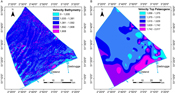
2.7.1. Time-to-depth conversion
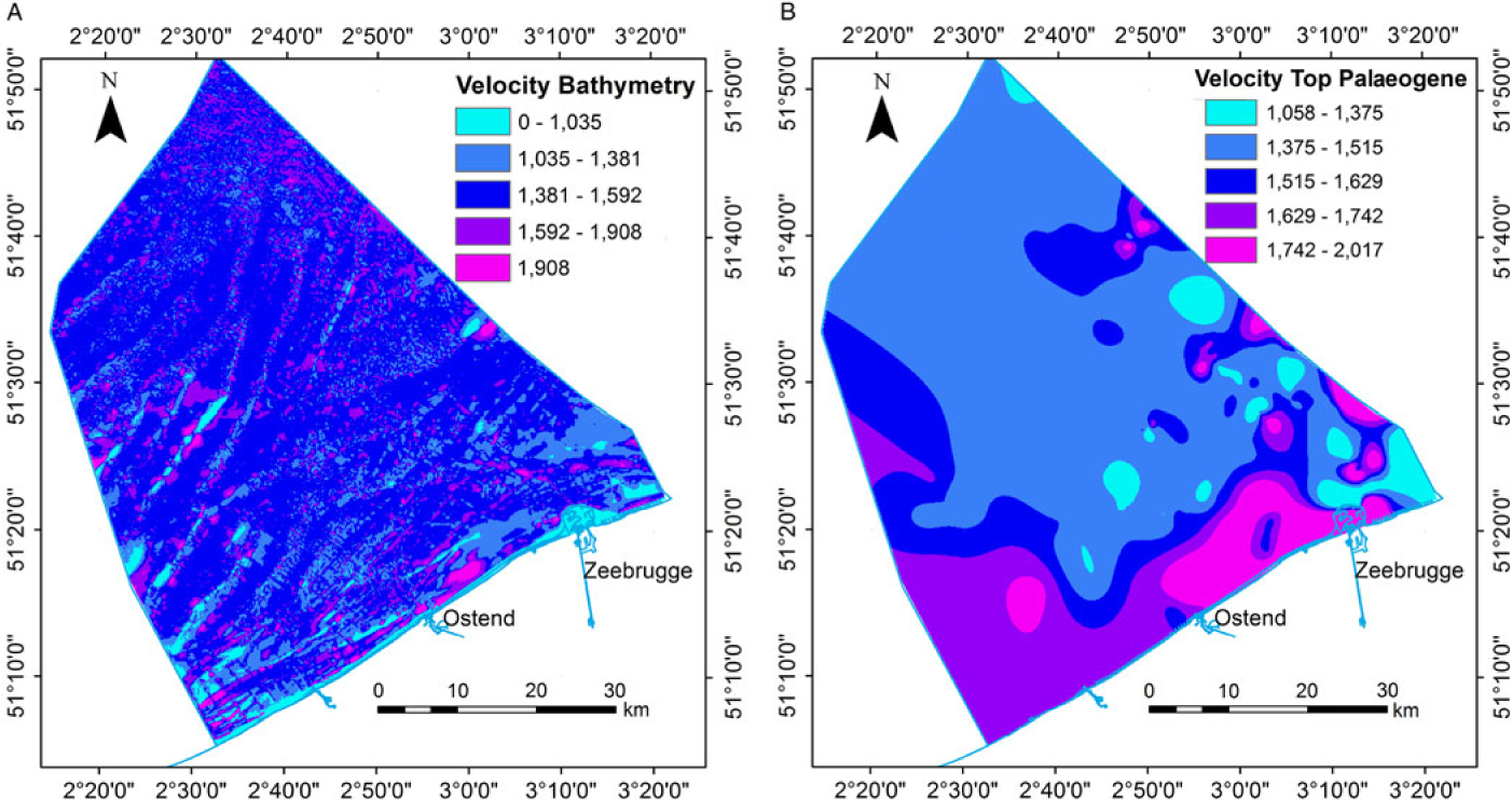
The horizons identified on seismic profiles were picked in time, because seismic traces are recorded in two-way travel time of the signal. A time-to-depth conversion is required to define the depth of the stratigraphic layers. In order to perform this conversion, the sound velocity within each layer was calculated. To achieve this and to validate the seismic interpretations, borehole and bathymetric data were incorporated and each seismic reflector was compared to the lithostratigraphical information from the cores. This allowed the creation of a velocity model (Fig. 4B) assigning a laterally varying internal velocity to each layer, rather than simply providing a constant value for the velocity of each layer. The laterally varying velocity model was used to calculate more accurately the Top-Palaeogene surface, the Top-Pleistocene surface and the Upper/Lower Holocene boundary. If a constant velocity model (e.g. 1500 m s−1) had been used, the thickness of the Quaternary units would have been locally over- or underestimated. Additionally, errors in depth caused by localised velocity anomalies due to morphological features such as the pull-up effect of sandbanks (Fagin, Reference Fagin1996) were addressed using this dynamic velocity model. Locally, the laterally varying velocity model based on the core dataset introduces artefacts such as depressions (e.g. in the Zeebrugge valley) that are not visible in or not covered by the seismic dataset. Other artefacts include unrealistically low velocity values in the water body related to the outcrop of the Palaeogene layer in between the sand banks (Fig. 4). Nonetheless, the core-based approach leads to better results than the constant velocity model which generally overestimates the depth of the top Palaeogene surface. Furthermore the velocity model, due to artefacts inherent in the nature of the dataset (digitised from paper, seismic lines), does not always refer to a physical velocity but is often a conversion factor.
Map showing the laterally varying velocity model in m s−1 used to calculate the depth of (A) the picked seafloor horizon (water column) and (B) the picked Top-Palaeogene horizon (Quaternary layer).
2.7.2. Geological layer creation
The depth of each seismic horizon was exported per line in a point format. Next, these points were interpolated by co-kriging using geostatistical software (ISATIS®), resulting in the creation of 2D bounding surfaces (grid size 200 × 200 m for the BCS and 100 m × 100 m for the Hinder Banks case study). All maps and models were vertically referenced to mean sea level (MSL). This reference level was chosen because it is calculated using onshore fixed points, while it also serves the need for a unified system between the Netherlands and Belgium in view of a future cross-border modelling programme. Since the Belgian seismic dataset and bathymetry were referenced to the lowest astronomical tide (LAT) they were converted to MSL using a grid provided by Deltares. Standard deviation of the surfaces was estimated using the co-kriging function and was subsequently used as a measure of uncertainty in the modelled stratigraphy.
The bounding surfaces were then combined to create the layer-based model defining the lithostratigraphical units (see step 5); cross-cutting between these surfaces has been resolved in seismic interpretation. The bathymetry (Flanders Hydrography) was used as the top surface.
2.8. Step 5: Assignment of lithostratigraphical units to the 3D voxel model
The next step is to define the volume in which the interpolation of lithological properties will take place. The highest point in the seafloor bathymetry was 4 m MSL (in the port of Zeebrugge), and the lowest point in the volume was −70 m MSL (corresponding to the bottom of the deepest borehole in the dataset). The grid resolution for modelling (i.e. the size of a single voxel) was set to 200 × 200 × 1 m (x, y, z), a choice based on data density and scale of the geological features that were described, while assuring a reasonable speed for the interpolation process. A higher-resolution model of 100 × 100 × 0.5 m was tested at the Hinder Banks.
The bounding surfaces, as described in step 4, are now added to the volume of the model, and the space between them is filled with voxels. The centres of the voxels (whether above or below a surface) define the lithostratigraphical unit they belong to. The voxels are assigned a constant integer value that corresponds to the lithostratigraphy (e.g. 1 for Nearshore Upper Holocene, 2 for Offshore Upper Holocene, etc.).
2.9. Step 6: 3D interpolation of lithological class
The next step in voxel modelling is to estimate a lithological class for each voxel, for which the Sequential Indicator Simulation (SIS) (Goovaerts, Reference Goovaerts1997; Chilès & Delfiner, Reference Chilès and Delfiner2012) technique was used (ISATIS®). SIS requires modest computation time and has been applied earlier in the creation of voxel models in similar geological settings (Stafleu et al., Reference Stafleu, Maljers, Gunnink, Menkovic and Busschers2011; Maljers et al., Reference Maljers, Stafleu, Van der Meulen and Dambrink2015).
Borehole data were first migrated to the closest voxel and considered as hard data afterwards. All the remaining voxels were scanned using a random path. A neighbourhood is established, centred on the target voxel, and within this neighbourhood the procedure searches for the hard data from the boreholes and for voxels that are already simulated. The neighbourhood is examined using a variogram model which ensures that data most closely correlated with the target voxels are assigned the greatest weight. The data are then coded into a set of indicators; hence the name indicator simulation. For each lithological class, the indicator is set to 1 if the data belong to the lithological class and to 0 if not. The next step in SIS consists of a co-kriging phase (block kriging) taking into account the previous information, resulting in a probability between 0 and 1 for each lithological class. The values are plotted in a cumulative distribution function. Then a random value between 0 and 1 is drawn and compared to the cumulative distribution function. The simulated lithological class at the target voxel corresponds to the rank of the interval to which the random value belongs.
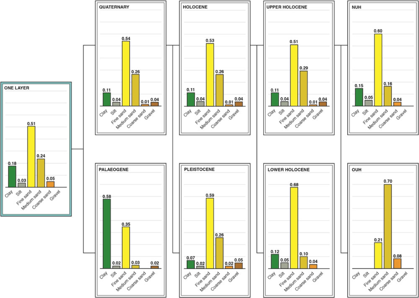
Especially in the deeper parts of the model, the neighbourhood search at a target voxel may end up with no data (neither hard data from boreholes nor already simulated voxels). The result is then drawn from proportions. These are the global proportions of each lithological class observed in the boreholes, which are assumed to be constant throughout the lithostratigraphical unit (Fig. 5).
Chart representing the global proportions of each lithological class in each lithostratigraphical layer in the process of adding more lithostratigraphical divisions in each model run (NUH: Nearshore Upper Holocene; OUH: Offshore Upper Holocene).
The SIS method can be extremely useful in relatively homogeneous geological units or in cases where good data coverage is available. However, on the BCS, and especially in the Holocene layer with its diverse sediment types, it may lead to errors in the form of so-called ‘flying’ voxels. These comprise voxels in regions of low data density that have been assigned a lithological class according to the global proportions (percentage of lithological class in each layer). This problem can be resolved by splitting the layer into smaller, better-defined sublayers. To allow a good comparison of the results, parameters such as the size of the neighbourhood (10 km) and the dimensions of the voxels (200 m × 200 m × 1 m) were kept constant as new lithostratigraphical layers were added.
The SIS resulted in 100, statistically equally probable, simulations of lithological class distributions. From these simulations probabilities of occurrence for each lithological class were calculated giving an indication of model uncertainty. In addition, the probabilities were used to compute a ‘most likely’ lithological class model using the averaging method for indicator datasets described by Soares (Reference Soares1992). However, the 100 individual simulation results remain available for further use.
2.10. Step 7: Assessment of the information entropy of the model
The probabilities of occurrence provide a measure of model uncertainty. Probabilities of an individual voxel can be displayed in a single bar chart, thus showing its probability distribution and hence model uncertainty. Similar displays are possible in visualisations of virtual boreholes (i.e. vertical stacks of voxels). However, in two- and three-dimensional visualisations (e.g. cross-sections or 3D views) it is not possible to show all probabilities for each voxel in a single view; the user will always be presented with one of the probabilities at a time.
To deal with this problem, Wellmann & Regenauer-Lieb (Reference Wellmann and Regenauer-Lieb2012) proposed the use of information entropy as a measure of uncertainty in 3D models. The information entropy of a voxel is a single value ranging from 0 to 1 that can be calculated from each of the probabilities of lithological classes. An entropy value of 0 means that there is no uncertainty, whereas a value of 1 occurs when all lithological classes have the same probability. Values in between 0 and 1 account for both the number of lithological classes with a probability higher than 0 (the more classes, the higher the entropy) and the differences amongst the probabilities (the greater the differences, the lower the entropy).
As suggested in Wellmann & Regenauer-Lieb (Reference Wellmann and Regenauer-Lieb2012), information entropy can be used as a quality measure of 3D models. In our study, information entropy is used as a comparative measure between different runs of the model. This comparison between the distribution of the information entropy helps quantify the effect of each layer addition on the model. Moreover, it allows us to visualise the overall quality of the model and make comparisons between the different interpolations.
3. Additional analyses
3.1. Stepwise improvement by adding layers
One of the aims of this study was to demonstrate how adding more geological information to the modelling process would improve the lithological characterisation of the lithostratigraphical units. As such, each borehole interval was attributed different levels of stratigraphy. For example, in the second run of the model when only two layers were used, the labels in the borehole descriptions are ‘Palaeogene’ and ‘Quaternary’, while in the last interpolation using five layers the core dataset contains the full set of relevant lithostratigraphical information (Nearshore Upper Holocene, Offshore Upper Holocene, Lower Holocene, Pleistocene, Palaeogene).
3.2. Hinder Banks case study: higher-resolution voxel modelling
Following the steps described above, a case study has been conducted on a smaller area with better data coverage. The case study area (see Fig. 3A) is located in the Hinder Banks area and comprises three major sandbanks (Noordhinder, Westhinder and Oosthinder). The dense bathymetric, seismic and borehole data coverage allowed the size of the voxels to be reduced to 100 × 100 × 0.5 m (x, y, z). The main reasons for choosing a higher voxel resolution were: (1) to test to what extent voxel size affects resource volume calculations; (2) to evaluate whether a higher resolution allows a better depiction of the different layers within the sandbanks; and (3) to compare the effects of different voxel sizes on the assigned lithological classes and probabilities of occurrence. The layers that are used for this test include the bathymetry, Top-Palaeogene and Top-Pleistocene; all three layers were interpolated at a resolution of 100 × 100 m, similar to the voxel size. The latter was achieved by re-interpolating the points from the seismic interpretation (cf. step 4). The Hinder Banks area is the main target for sand dredging in the years to come (Mathys et al., Reference Mathys, Van Lancker, De Backer, Hostens, Degrendele and Roche2011); as such, an accurate estimate of the resource volume and lithology is crucial.
4. Results
Five different units were distinguished defining the lithostratigraphical succession in the BCS: Palaeogene, Pleistocene, Lower and Upper Holocene, the latter with a subdivision into Nearshore and Offshore. Results are presented on the five model runs starting from the use of a uniform stratigraphy in the modelling process up to using all five units. This was done to compare the effects of the addition of each unit to the model. Additionally, the workflow was applied in a higher resolution in an area with higher data coverage. Results become progressively more detailed as the introduction of each new lithostratigraphical layer divides the model into smaller segments.
4.1. Lithological and stratigraphical framework
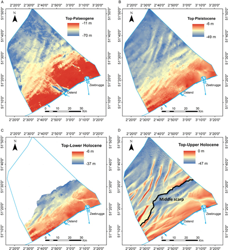
The 2D bounding surfaces, that were created in step 4 of the methodology section, are shown in Fig. 6. When overlaid, they form the top and bottom of each unit that will be used in the different interpolations. The space between them is filled with voxels. The voxelised lithostratigraphical units and their extent can be seen in Fig. 7.
Views of the modelled bounding surfaces used in the voxel modelling. (A) Top-Palaeogene, (B) Top-Pleistocene, (C) Top-Lower Holocene and (D) Top-Upper Holocene (bathymetry), the latter with a subdivision into Nearshore and Offshore defined by the Middle Scarp.

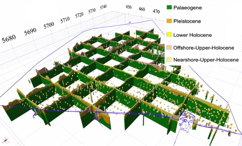
Fence diagram of voxelized lithostratigraphical units in the BCS. The borehole dataset is colour-coded following their lithostratigraphical interpretation. The blue line represents the extent of the modelled area.
Results show that the Quaternary cover is very thin and its sediments are accumulated mainly in the sandbanks. Each sandbank is unique in its stratigraphical and lithological content. This makes the modelling procedure more challenging because these geological features and their internal structure must be taken into consideration when splitting a lithostratigraphical unit. Fig. 7 shows the results of the lithostratigraphical characterisation of the borehole dataset, as discussed in step 5.
The level of detail even in the 200 × 200 m resolution of the surfaces allowed the robust modelling of the different geological units described previously, taking into account the stratigraphical boundaries and features (Fig. 6) of the Quaternary cover. For example the extent of the Ostend valley is 10 × 5 km; its internal features can be described well by a 200 × 200 m resolution model. Other resolutions have been tested for the BCP model, though based on the data density and calculations time the 200 × 200 m resolution was decided upon as the most effective. All of these geological features are clearly visible in each unit, such as the sandbanks and the platform in the Holocene and the Ostend Valley in the Pleistocene.
4.2. Stepwise incorporation of geological knowledge
4.2.1. Single-layer model (uniform stratigraphy)
In the single-layer model, the volume in which the 3D interpolation of lithological class takes place is bounded only by the bathymetry (in MSL) at the top and a horizontal boundary at −70 m MSL. The lithological classes of the borehole dataset were used without stratigraphical interpretation.
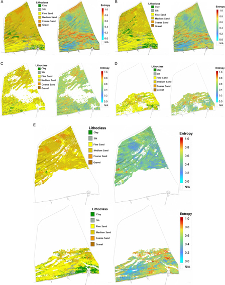
The results for the single-layer model are shown in Fig. 8A. The model seems to work well in the area around Zeebrugge due to the good data coverage and where the model clearly shows the transition from Palaeogene clays to Quaternary sands. Although no stratigraphic information was added to the model, the model still correctly predicts clay in the depth intervals that contain Palaeogene layers, and sand in the depth intervals that contain Quaternary layers. In other parts of the BCS, with much lower data coverage, the lithological class ‘sand’ is wrongly propagated into the Palaeogene layer due to the global proportion of sands (see Fig. 5, in blue) in the borehole dataset. The model uncertainty map on the right shows high uncertainties (red voxels) in many areas.
Top view of the different runs of the model. Left: lithoclass. Right: distribution of the entropy. (A) Uniform stratigraphy (no bounding surfaces defining the stratigraphy). (B) One bounding surface (Top-Palaeogene). (C) Two bounding surfaces (Top-Palaeogene and Top-Pleistocene), defining three lithostratigraphical layers of which only the Pleistocene is shown here. (D) Three bounding surfaces (Top-Palaeogene, Top-Pleistocene and Lower Holocene) defining four lithostratigraphical layers of which only the Lower Holocene is shown here. (E) Four bounding surfaces (Top-Palaeogene, Top-Pleistocene, Lower Holocene, Nearshore Upper Holocene, Offshore Upper Holocene), defining five lithostratigraphical layers of which the Nearshore (bottom) and Offshore Upper Holocene (top) are shown here.

4.2.2. Two--layer model (Palaeogene–Quaternary)
The first surface added to the model was the Top-Palaeogene unconformity (De Clercq et al., Reference De Clercq, Chademenos, Van Lancker and Missiaen2016). It is the bounding surface between the Palaeogene and the overlying Quaternary deposits and constrains the lower boundary of the resource units, and as such it has a significant impact on the resource calculations. The results of the two-layer model are shown in Fig. 8B. The Top-Palaeogene layer is now defined as consisting of 56% of clay (see Fig. 5, in green). Moreover, as the Top-Palaeogene surface comprises complex geomorphological features, abrupt lateral changes in the sediment composition are now much better constrained. A good example is the Ostend Valley (Fig. 1) cutting into the underlying clay sediments (Fig. 15).
4.2.3. Three-layer model (Palaeogene–Pleistocene–Holocene)
The second added surface is the Top-Pleistocene surface, allowing differentiation of Quaternary deposits in terms of their lithological composition. The patchy and lithologically mixed Quaternary layer comprises the infill of the palaeovalleys in the nearshore area of the BCS, and forms the core of the sandbanks in the offshore area (see Fig. 1). The results of the three-layer model for the BCS are shown in Fig. 8C. In the Ostend Valley, for example, fine sands can now be distinguished from overlying clay sediments.
4.2.4. Four-layer model (Palaeogene – Pleistocene – Lower Holocene – Upper Holocene)
In the nearshore, one extra layer was added to account for the lithological differentiation in the Lower Holocene which is here related to a fine-grained tidal-flat environment (Mathys, Reference Mathys2009). Further offshore, the Holocene deposits are coarser. The main purpose of adding this layer was to demonstrate the sensitivity of the model in describing a lithologically varying layer with very few cores crossing it. The results of the four-layer model are shown in Fig. 8D.
4.2.5. Five-layer model (Palaeogene – Pleistocene – Lower Holocene – Nearshore Upper Holocene – Offshore Upper Holocene)
In the final model, the Upper Holocene layer was further split (laterally) into two smaller areas. This was done primarily because of the increasing presence of medium sand further offshore as well as to reduce the presence of ‘flying’ clay voxels that were present in the Holocene layer of the three-layer model (Top-Pleistocene surface). These ‘flying’ voxels were introduced by the SIS as the global proportions of the clay–silt percentages were forced through the entire model (see Fig. 5). Clay–silt percentages are significantly higher in the nearshore area, because of the nearby estuary of the Scheldt river. In order to separate the two regions (with and without Scheldt influence), the Middle Scarp (see Fig. 1) was used as proxy where the depositional environment changes from a nearshore estuarine–marine to an offshore marine environment. The results of the five-layer model are shown in Fig. 8E.
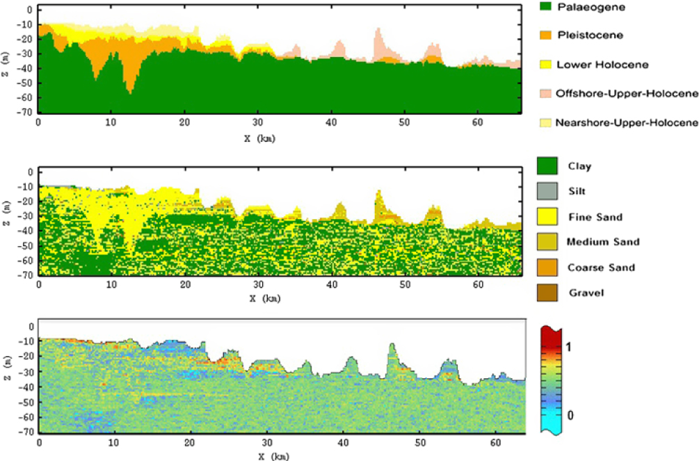
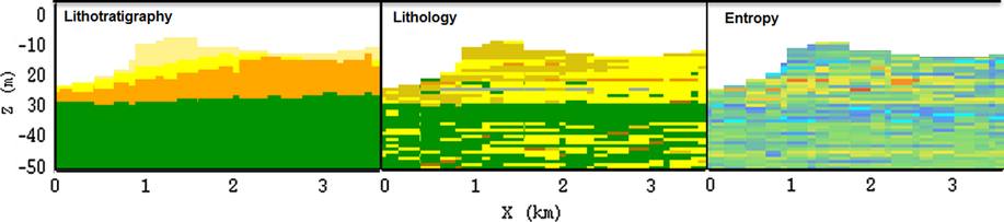
Another way of querying the model is the creation of cross-sections (Fig. 9). This type of data visualisation allows inspection of the in-depth distribution of the different assigned variables. Following the geological cross-section of Fig. 1, we can see all five lithostratigraphical units with the assigned lithology and information entropy. Cross-sections like these give a first glimpse of the areas where we are confident of the assigned lithology (blue colour in bottom figure), e.g. the fine sand above the Ostend Valley and the coarse sand tips off the Hinder Banks.
Cross-section of the final model (for location, see Fig. 1). Top: lithostratigraphical units. Middle: lithological class. Bottom: model entropy on the lithological class. 0 indicates low and 1 high uncertainty.
5. Case study with higher resolution of the voxel model
The analysis of the results of the case study gives a detailed overview of the lithological properties of the area. The 100 × 100 × 0.5 m voxel model shows a predominance of medium sand (Fig. 10). A major difference with the 200 × 200 × 1 m resolution five-layer model is the detailed lithological variation within the sandbanks. The 100 × 100 × 0.5 m was chosen based on the data density. The sandbanks are characterised by a Pleistocene core of coarse sand and gravel, mixed with clay and silts. The silt is mainly found in the upper part of the Pleistocene layer forming a transition boundary towards the Offshore Upper Holocene layer. Coarse sand and gravel populate the space between the sandbanks as well. Moreover, the Palaeogene layer is now composed almost completely of clay since the limited number of cores that penetrate the Palaeogene layer in the Hinder Banks have a global proportion of 92% clay.
High-resolution voxel model (100 × 100 × 0.5 m) of the Hinder Banks. Left: lithological class. Right: model entropy for the lithological class, shown only for the Quaternary.
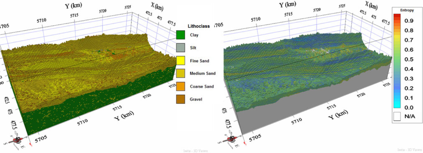
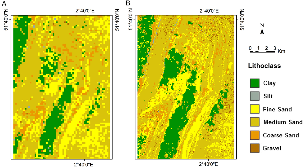
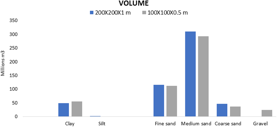
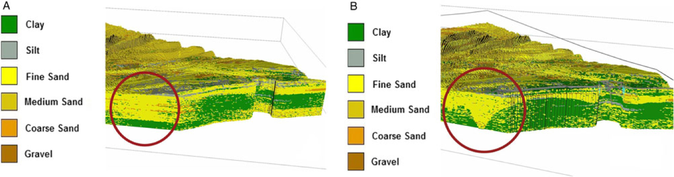
To compare the resource volumes between the different resolution models of the Hinder Banks, resource quantity was queried in the first 2 m below seafloor (Fig. 11). The different resolutions do not affect the total volume of the queried voxels. However, there is a difference when comparing the lithologies of the two models (Fig. 12). This difference is due to the fact that in the 100 × 100 × 0.5 m resolution model the core dataset used is confined to a buffer zone around the modelled area, while in the 200 × 200 × 1 m resolution model the core dataset of the entire BCS (Fig. 3) is used. This clearly influences the voxels assigned with gravel, since the percentage of gravel is much higher in the cores around the Hinder Banks compared to the BCS dataset. Another advantage of the higher-resolution model is the fact that the lithostratigraphical units are much better defined, as shown by the Pleistocene inner core of the sandbanks. Additionally, some features were better delineated, e.g. the fine sand in the top zone of one of the sandbanks which is present in both models.
Queried volumes of the first 2 m of sediment in the Hinder Banks area. (A) 200 × 200 × 1 m resolution. (B) 100 × 100 × 0.5 m resolution.
Queried volumes comparison of the first 2 m of sediment in the Hinder Banks area.
Example of a seismic reflection profile and interpreted seismostratigraphical units. From Trentesaux et al. (Reference Trentesaux, Stolk and Berne1999: Fig. 3, p. 256).
6. Discussion
6.1. Importance of geological knowledge in voxel modelling
Modelling the subsurface geology of shallow marine environments is highly challenging because of the complex depositional environments that often vary on short spatial scales. Detailed interpolation of lithological information is hence critical and requires the best available knowledge on the geological layers constraining different resource qualities.
For the BCS, the Middelkerke Bank (localisation, see Fig. 1) was the first sandbank from which the succession of geological layers was defined (Trentesaux et al., Reference Trentesaux, Stolk and Berne1999). Fig. 13 shows the original seismic line and its interpretation, based on the combination with the boreholes. The same information was now used in the voxel modelling. Compared to the previous interpretations, we are now able to model the lithological distribution, as well as the related information entropy of the model (Fig. 14). The higher values of information entropy can be seen in the centre of the sandbank associated with the uncertainty caused by the lack of cores.
Left: lithostratigraphical units. Middle: lithological class. Right: model uncertainty, as queried from the voxel model along the same cross-section of Trentesaux et al. (Reference Trentesaux, Stolk and Berne1999; see Fig. 13). For values see legend of Fig. 9.
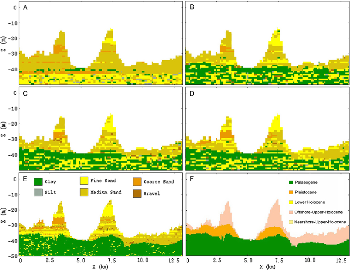
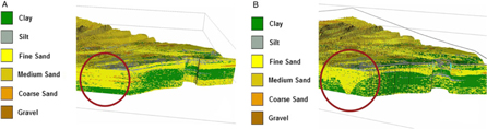
By visualising and querying the different models, the effects of the changes are discussed and evaluated. As a first example, the effect of a better parameterisation of the Top-Palaeogene is shown in Fig. 15. This was most striking for the delineation of the Ostend palaeovalley in the nearshore zone. In the single-layer model, fine sand voxels extended horizontally and masked the boundary of the valley. With the addition of the Top-Palaeogene surface, a distinct V-shape of the palaeovalley became apparent and allowed showing an infill of the valley with fine-sand (yellow) voxels above the Palaeogene clay layers. A second example illustrates the dramatic change that the addition of layers can make to the distribution of the lithological classes (Fig. 16). This is most evident on the level of the sandbanks (e.g. Hinder Banks) where in the second run of the model the base of the sandbank is better defined because of the addition of the Top-Palaeogene surface. In the third run of the model the introduction of the Pleistocene unit allowed us to define a core of lithologically mixed sediments. Finally, the fifth run of the model allowed us to differentiate layers of different lithological classes in the main body of the sandbanks once the offshore Upper Holocene unit was defined. The final figures illustrate that more data allow the creation of higher-resolution models that constrain better the stratigraphical layers and their lithological properties.
The effect of adding the Top-Palaeogene bounding surface in the area of the Ostend Valley, a buried valley in the nearshore area. (A) Uniform stratigraphy model. (B) One-layer model.
Cross-section in the area of the Hinder Banks showing the distribution of lithoclasses of the different runs of the 200 × 200 × 1 m model. (A) One-layer model (no bounding surfaces). (B) One bounding surface (Top-Palaeogene). (C) Two bounding surfaces (Top-Palaeogene and Top-Pleistocene). (D) Four bounding surfaces (Top-Palaeogene, Top-Pleistocene, Lower Holocene, Nearshore Upper Holocene, Offshore Upper Holocene). Followed by the final results from the 100 × 100 × 0.5 m resolution model. (E) lithological class, and (F) lithostratigraphical units.
The addition of geological layers also allowed the reduction of the number of ‘flying voxels’, that were introduced as a consequence of the SIS method. In areas with low data density, SIS draws the lithological class from the global proportions per lithostratigraphical unit. By splitting the model volume into separate lithostratigraphical units, these percentages change according to the lithological content of the boreholes belonging to the lithostratigraphical units. In the Offshore Upper Holocene layer, as depicted in Fig. 15B, there is significantly less clay–silt in the global proportions (Fig. 5) when split from the Upper Holocene. As a result of the lower percentages, the majority of ‘flying voxels’ (Fig. 15A) are no longer present.
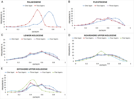
To quantify the added value of incorporating geological knowledge in the voxel modelling procedure, the model uncertainty calculations, performed on each of the model runs, are now discussed and compared (Schweizer et al., Reference Schweizer, Blum and Butscher2017). Fig. 17 shows distribution curves of the model uncertainty with each new addition of a geological layer.
Distribution of the model entropy on the lithological class for each layer queried for different runs of the model. 0 indicates low and 1 high uncertainty.
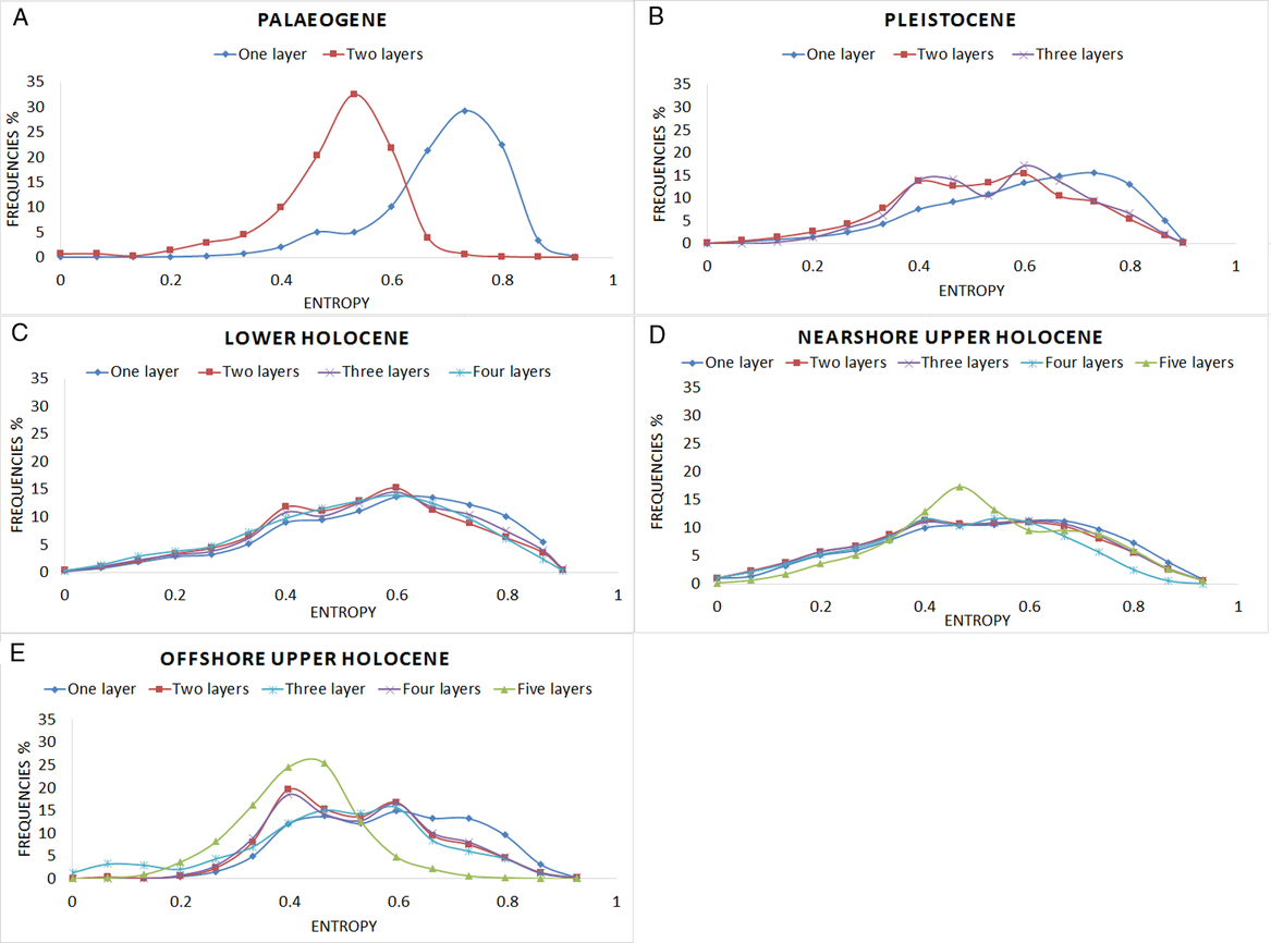
In the single-layer model (first run – blue line) the mean of the model uncertainty distribution is close to 0.7 (Fig. 17A). Adding the Quaternary layer (second run – red line), the mean is close to 0.5, indicating an improvement of the modelling of the Palaeogene layer. The different runs of the model did not have the same pronounced effect on the model uncertainty distribution of the Pleistocene layer (Fig. 17B). Also, the addition of the Lower Holocene layer did not show any improvement in the model uncertainty distribution of the model (Fig. 17C). This can be attributed to the fact that this layer is poorly described in the cores and that there are no distinct differences in the lithological content that the addition of the lithostratigraphical layer can describe.
Adding the Nearshore Upper Holocene layer resulted in a more distinctive peak in the model uncertainty spectrum (Fig. 17D – green line). The high values of model uncertainty (0.6–0.8) are caused by the complex geology of the Scheldt estuary. The presence of laminated layers consisting of clay and fine sand makes it difficult for the method to predict the lithology of the voxels in the region, at least at the scale of the present model.
The Offshore Upper Holocene layer shows two distinct peaks (0.5 and 0.65) in the model uncertainty spectrum in the second and third runs of the model (Fig. 17E – red, light blue and purple lines). When the Holocene layer is split in the fifth run of the model (green line), the model uncertainty improves (peak around 0.4). This is because the offshore sandbanks have a better data coverage than the areas in the gullies between the sandbanks, where the information entropy is higher (0.5–0.7).
6.2. Future perspectives
The model provides the uncertainty (information entropy) of the lithological class in each voxel based on the calculations of the SIS method. However, this uncertainty is now solely related to statistical calculations, whilst there is also uncertainty imposed by the dataset itself. Data-related uncertainties include those originating from the seismic lines (bad quality, misplacement) and borehole descriptions (mislabelling, insufficient interpretations, inadequate metadata) datasets and may have an adverse effect on the confidence we have in the resulting model. These uncertainties have already been quantified and incorporated in the model as flags, and procedures are now evaluated on how to propagate those uncertainties in the voxel models (De Tré et al., Reference De Tré, De Mol, Van Heteren, Stafleu, Chademenos, Missiaen, Kint, Terseleer, Van Lancker, Bordogna and Carrara2018). The areas with high uncertainty help us to understand the limitations of the datasets and will guide the planning of new data acquisition surveys.
With increasing use of the BCS, both by the public and private sector, there are ample opportunities to validate and apply the model for different purposes, ideally by incorporating new data. Some of these applications may require a higher vertical resolution, which will require more tests. With the 1 m vertical scale resolution, certain features such as the clay–silt–fine-sand laminated layering in the estuarine deposits are easily overlooked, especially in regions with high lithological heterogeneity. A case study close to the port of Zeebrugge has been planned where the resolution will be decreased to 0.7–0.4 m. In this area, it is also planned to incorporate additional data, such as cone penetration tests, making the model more valuable for geotechnical applications.
Last but not least, it needs emphasising that the model is the backbone of a resource decision support system (Van Lancker et al., Reference Van Lancker, Francken, Kint, Terseleer, Van den Eynde, De Mol, De Tré, De Mol, Missiaen, Hademenos, Bakker, Busschers, Maljers, Stafleu, Van Heteren, Diviacco, Leadbetter and Glaves2017). As such, users have direct access through the TILES website to the available geological information and can query resource quality and quantity, in combination with environmental and socio-economic datasets, in view of different applications, now and in the future.
7. Conclusions
A 3D voxel model was created depicting in detail stratigraphical and lithological information of the subsurface of the BCS. The 3D environment allows easy viewing of geological properties providing spatial context to certain features or heterogeneities in the subsurface, which is highly valuable in resource management. Geological knowledge was incorporated in a stepwise approach and gave a level of detail in the model that would not have been achieved by only using available coring data. Moreover, the stepwise approach allowed us to monitor the effect of each layer addition on the model and its effectiveness in describing the geological features. In addition, model uncertainty, calculated as information entropy, was added to the voxels, providing insight into how successful the model is in unambiguously estimating lithological classes. Because of the automated workflow, new data can be incorporated easily and results can be compared and evaluated against previous versions of the model.
The new voxel model forms the backbone of a resource decision support system allowing structured querying of extractable aggregate resource volumes combining the geology-related information (stratigraphy, lithological class, model uncertainty) and any third party data that may constrain exploitation (e.g. shipping lanes, cable lines, port locations, ecologically valuable areas).
Author ORCIDs
Vera Van Lancker 0000-0002-8088-9713
Acknowledgements
This paper is a contribution to the Brain-be project TILES (Transnational and Integrated Long-term marine Exploitation Strategies), funded by Belgian Science Policy (Belspo) under contract BR/121/A2/TILES, and the Flemish research project SeArch (IWT SBO, contract nr. 120003). The research is fully supported by the ZAGRI project, a federal Belgian programme for continuous monitoring of sand and gravel extraction, paid from private revenues. Contributing EU projects have been EMODnet Geology (MARE/2008/03; MARE/2012/10; EASME/EMFF/2016/1.3.1.2 – Lot 1/SI2.750862)), Geo-Seas (FP7, Grant 238952) and ODIP (FP7, Grant 312492). Underlying data have been acquired during numerous campaigns on RV Belgica, RV Simon Stevin and many Dutch research and monitoring vessels. For Belgian waters, ship-time was granted by Belspo / RBINS ODNature and Flanders Marine Institute. Nikki Trabucho, TNO, is acknowledged for the graphical design of Figures 2 and 5. The Federal Public Service Economy, Continental Shelf department is thanked for continuous support. Results, datasets, findings and the final version of the models are available through https://odnature.naturalsciences.be/tiles/. Dr P. Kruiver and an anonymous reviewer are thanked for very constructive comments.


 Open access