


Nomenclature
- ATR
-
active twisting rotor
- BVI
-
blade vortex interaction
- CFD
-
computational fluid dynamics
- CFL
-
Courant–Friedrichs–Lewy
- CSD
-
computational solid dynamics
- FE(M)
-
finite element (method)
- HVAB
-
hover validation and acoustic baseline
- HPW
-
American Institute of Aeronautics and Astronautics (AIAA) hover prediction workshop
- MFC
-
macro fibre composite
- SST
-
shear stress transport
- STAR
-
smart twisting active rotor
- URANS
-
unsteady Reynolds averaged Navier–Stokes
- ${\alpha _i}$
-
generalised coordinate of mode i
-
$\theta $
,
${\theta _0}$
-
blade collective angle with reference to 75% of radius, degrees
-
${\theta _{tw}}$
-
rotor blade twist distribution, degrees/R
-
${\theta _{tw,el.}}$
-
pitch-up torsion deformation, degrees
-
${\rho _{\left( \infty \right)}}$
-
(free stream) density,
${\rm{kg}}/{{\rm{m}}^3}$
-
${\phi _i}$
-
mode shape vector array of mode i
-
$\sigma $
-
rotor solidity,
$R\pi /\left( {{N_B}c} \right)$
-
${\zeta _i}$
-
damping ratio of mode i
-
${\omega _{\left( i \right)}}$
-
frequency (of structural mode
$i$
),
$1/{\rm{s}}$
-
${\rm{\Omega }}$
-
rotor rotational speed,
$1/{\rm{s}}$
-
${{\rm{\Omega }}_{\left( 0 \right)}}$
-
rotor (reference) rotational speed,
$1/{\rm{s}}$
-
${\nu _i}$
-
Poisson’s ratio for orthotropic directions
$i$
-
${a_\infty }$
-
speed of sound,
${\rm{m}}/{\rm{s}}$
-
$c$
-
rotor blade chord, m
-
${C_n}$
,
${C_m}$
-
sectional normal force and moment coefficients,
$d{C_N}/d\left( {r/R} \right)$
,
$d{C_M}/d\left( {r/R} \right)$
-
${C_Q}$
-
coefficient of rotor torque,
$Q/\left( {\pi {\rho _\infty }V_{tip}^2{R^3}} \right)$
-
${C_T}$
-
coefficient of rotor thrust,
$T/\left( {\pi {\rho _\infty }V_{tip}^2{R^2}} \right)$
-
${E_i}$
-
Young’s modulus in direction
$i$
, GPa -
$FoM$
-
figure of merit,
$C_T^{3/2}/( {\sqrt 2 {C_Q}} )$
-
${f_i}$
-
aerodynamic forces projected on structural mode
$i$
-
$F_x^i$
-
periodic forcing component x at time step
$i$
-
${F_{x,n}}$
-
${n}^{\rm{th}}$
Fourier decomposition amplitude of x-axis force component, N
-
${G_i}$
-
shear modulus in plane
$i$
, GPa -
$M$
/
${M_{tip}}$
-
local/tip Mach number
$V/{a_\infty }$
/
${V_{tip}}/{a_\infty }$
-
${M_{x,n}}$
-
${n}^{{\rm{th}}}$
Fourier decomposition amplitude of moment around x-axis, Nm
-
${N_B}$
-
number of rotor blades
-
$Q$
-
rotor torque, Nm
-
${Q_{crit}}$
-
Q-criterion
-
$r$
-
rotor section radial position, m
-
$R$
-
rotor blade radius, m
-
$T$
-
rotor thrust (shaft-axis upward), N
-
${V_{tip}}$
-
rotor tip speed, m/s
-
$x,y,z$
-
rotor in-plane axes, coordinate positions, m


1.0 Introduction
Helicopters play an important role in civilian and military applications due to their ability to hover at high payloads and their exceptional manoeuvrability. Since their inception, the main goals of helicopter research have been to improve the payload capacity, range and endurance, and to reduce vibration and noise emissions. The forces and moments on the helicopter are mostly generated by the main rotor(s). Rotors consist of several spinning blades with cyclic control, and their flow is time-dependent. The resulting periodic forcing component is the main source of vibrations; however, interactions between rotor blades, tail rotor and fuselage also contribute. Specifically, interactions of the blades with the tip vortices can have a large impact on the forces, moments, and consequently vibration. The unsteady load components are dominated by multiples of the blade passing frequency (BPF). Such vibrations are transmitted to the airframe and cause structural fatigue and passenger discomfort, and therefore need to be limited. Reichert [Reference Reichert1] suggests airframe vibrational accelerations of less than $0.02{{\;g}}$
for passenger comfort. The largest vibration amplitudes occur in transitional flight from hover to cruise and high-speed flight. The former is due to the unsteady rotor inflow field from turbulence ingestion and tip vortex interactions. High-speed flight vibrations are mainly due to the large force distribution differences between advancing and retreating sides of the rotor disk, in conjunction with rotor blade twist, producing regions of reversed flow and locations with almost sonic Mach numbers. On-blade actuators for higher-harmonic control have been demonstrated for improved vibration control, noise attenuation and fuel efficiency. Examples of this are numerical and experimental works for active flaps [Reference Millott and Friedmann2–Reference Straub, Anand, Lau and Birchette5], morphing trailing edges [Reference Mistry and Gandhi6], Gurney flaps [Reference Woodgate, Pastrikakis and Barakos7, Reference Pastrikakis, Steijl and Barakos8] and discontinuous varying blade tips [Reference Bernhard and Chopra9, Reference Bernhard and Chopra10]. Furthermore, active twist systems are presented in review papers [Reference Loewy11–Reference Shivashankar and Gopalakrishnan14]. Blade-integrated torsion actuators are considered in this study, due to their advantages, for example, their resistance to airborne sand and snow, and benefits in icing conditions. For the development and certification of such devices, accurate simulation tools are needed. Because of the inherent couplings between in-plane and out-of-plane structural deformations, the in-house Helicopter Multi Block 3 (HMB3) Navier-Stokes fluid dynamics solver is coupled to the commercial finite-element structural solver MSC NASTRAN. A conventional 1D beam model, derived from numerical cross-section data, is compared to a 3D finite element (FE) model, created from geometry and material data, to determine which tools are suitable for accurate simulations of rotor blades with blade-integrated piezoelectric actuators.
$0.02{{\;g}}$
for passenger comfort. The largest vibration amplitudes occur in transitional flight from hover to cruise and high-speed flight. The former is due to the unsteady rotor inflow field from turbulence ingestion and tip vortex interactions. High-speed flight vibrations are mainly due to the large force distribution differences between advancing and retreating sides of the rotor disk, in conjunction with rotor blade twist, producing regions of reversed flow and locations with almost sonic Mach numbers. On-blade actuators for higher-harmonic control have been demonstrated for improved vibration control, noise attenuation and fuel efficiency. Examples of this are numerical and experimental works for active flaps [Reference Millott and Friedmann2–Reference Straub, Anand, Lau and Birchette5], morphing trailing edges [Reference Mistry and Gandhi6], Gurney flaps [Reference Woodgate, Pastrikakis and Barakos7, Reference Pastrikakis, Steijl and Barakos8] and discontinuous varying blade tips [Reference Bernhard and Chopra9, Reference Bernhard and Chopra10]. Furthermore, active twist systems are presented in review papers [Reference Loewy11–Reference Shivashankar and Gopalakrishnan14]. Blade-integrated torsion actuators are considered in this study, due to their advantages, for example, their resistance to airborne sand and snow, and benefits in icing conditions. For the development and certification of such devices, accurate simulation tools are needed. Because of the inherent couplings between in-plane and out-of-plane structural deformations, the in-house Helicopter Multi Block 3 (HMB3) Navier-Stokes fluid dynamics solver is coupled to the commercial finite-element structural solver MSC NASTRAN. A conventional 1D beam model, derived from numerical cross-section data, is compared to a 3D finite element (FE) model, created from geometry and material data, to determine which tools are suitable for accurate simulations of rotor blades with blade-integrated piezoelectric actuators.
Rotor blade structural design is a significant challenge, with aerodynamicists targeting thinner and higher aspect ratio rotor blades. Achieving the required bending and torsional rigidity, along with the desired neutral axis, elastic axis and centre of gravity locations within a given outer mould line, competes with the goal of decreasing the blade weight. Due to the centrifugal stresses, any additional blade mass also requires additional strength, hence amplifying the problem. Blade structural designs are validated either by FE method (FEM) models or by sectional analyses. Modern cross-section and beam-coupled methods iterate on an inner loop to account for warping and deformations of the sections.
In the 1990s and 2000s, comprehensive rotor codes using lifting line theories with 1D beam structural coupling identified difficulties predicting the vibration, pitch link loads and aerodynamic loads in transonic, negative lift or reversed flow regions. Accurately capturing the force and moment variations is vital to calculating vibration metrics and structural stresses. The blade tip torsion also has a significant impact on these metrics; therefore, predicting the aerodynamic pitching moments is crucial. Replacing the simplified aerodynamic tools with computational fluid dynamics (CFD) helped predict rotor loads and thereby hub vibrations, especially in difficult conditions, such as high lift, high advance-ratio and blade vortex interaction (BVI) cases. One-dimensional beam model approaches are commonplace in rotorcraft analyses. These models are often part of rotor dynamics and trimming toolboxes, which are integrated with mid-fidelity and high-fidelity CFD solvers. Because of the strong historical integration between the codes, significant effort is needed to open the toolboxes to structural analyses using 3D FE approaches.
Many different implementations of FE beam structural models are reported in the literature. The history and underlying principles of such beam models are explained by Hodges [Reference Hodges15], who also proposed a thorough and applicable model for helicopter rotor blades. Such models are usually as accurate as 3D FEMs for the slender sections with relatively constant cross-section, but less accurate in the geometrically complex blade-root and load-path regions. These regions, however, are usually very stiff, which reduces the influence of such errors on the overall result. Non-linear beam models must be integrated with cross-sectional analysis tools to account for effects such as in-plane or out-of-plane warping and stress concentrations. The commercial solver used in this work is not integrated with cross-sectional analysis and therefore suffers from the associated problems, which are especially relevant for composite beams.
An advantage of the beam model approach is its low computational cost. Cross-sectional meshes or calculated properties can be tweaked relatively easily, if necessary, to match an experiment. However, it can still be difficult to tweak beam models of blades with strong cross-coupling between modes, due to spanwise variations and effects of the centrifugal force. A disadvantage of this modelling type is that it relies on cross-sections, which are in the radial plane. It is therefore less suited for complex, manufactured rotor blades, with associated manufacturing deviations.
With a large increase in computational expense and meshing effort, the root and aerofoil portions of the rotor blade can be analysed using the 3D FEM. This method allows to directly model on-blade actuators with their complex geometries and deals more easily with material properties and geometry variations.
Ideally, the 3D structural models can be directly converted from computer-aided design (CAD) and manufacturing data, as is the case in this study. Developing FEM models using 3D computer tomography can help with validation and to quantify deviations from numerical results of models with perfect manufacturing [Reference Ahn, Hwang, Chang, Jung, Kalow and Keimer16]. With additional data on part positioning, manufacturing variations and coupon-checked material properties, an almost perfect digital replica can be produced for the simulations. However, making adjustments to 3D models is more difficult than to beam and cross-section models. Changes in geometry are time-consuming because the FE mesh quality must be preserved. Changes to any material or geometric properties usually affect all isolated and coupled deformation modes.
Because of the computational cost and complexity, 3D FE structural analysis has not been coupled to rotorcraft CFD – until recently. Even outside of rotorcraft, CFD-FEM coupling is limited in its application to non-rotating parts. Often, this process is reduced to a CFD computation for the fluid loads, followed by an FEM calculation of the structural stresses, without iterations. Over the last decade, an FE 3D structural solver was developed and integrated with the CREATE-AV HELIOS rotor CFD code [Reference Datta17] in a framework called X3D. Periodic structural deformations were obtained using a modified harmonic balance method FE solver. The FE solver is based on the linearised structural equation of motion with a forcing function: ${\boldsymbol{{M}}} \ddot x + {\boldsymbol{{C}}} \dot x + {\boldsymbol{{K}}} x = {\boldsymbol{{F}}}$
. A more-than 8
${\boldsymbol{{M}}} \ddot x + {\boldsymbol{{C}}} \dot x + {\boldsymbol{{K}}} x = {\boldsymbol{{F}}}$
. A more-than 8 $ \times $
speedup compared to the previous, parallelised, time-marching FEM structural solver was demonstrated and applied to a UH-60A forward flight case [Reference Patil and Datta18].
$ \times $
speedup compared to the previous, parallelised, time-marching FEM structural solver was demonstrated and applied to a UH-60A forward flight case [Reference Patil and Datta18].
A loose coupling similar to delta airloads was used. Its implementation is similar to that described in Ref. [Reference Potsdam, Yeo and Johnson19]. The rotor aeroelasticity and trimming solution is obtained using a free-wake lifting line method. The ‘delta-airloads’ are the difference between CFD and lifting line airloads, which are considered in the following trimming and deformation recalculations and iterations. Once a periodic solution is obtained, the lifting line loads cancel, and one is left with the aerodynamic forces.
After validating the method, Patil et al. [Reference Patil, Lumba, Jayaraman and Datta20] showed how blade-bending stresses could be obtained from FEM in the aeroelastic-coupled and trimmed simulation of an open-source coaxial rotor, modelled after the Sikorsky S-97 Raider. The X3D model of this Metaltail-II rotor blade was made of multiple rigid and deformable parts. The blade and connector meshes exclusively used 27-vertex brick elements, resulting in $\tilde 6$
900 degrees of freedom (DoF) per blade. The element vertices did not coincide with the aerodynamic mesh, as the structural mesh is much coarser. For the work on the co-axial rotor, the data between CFD and computational solid dynamics (CSD) were exchanged by interpolation on the quarter chord line. In this approach, the usually negligible in-plane deformations are lost. Deformations of the blade aerofoil cross-section could therefore not be modelled. The University of Maryland is planning to implement a 3D exchange method in its code, which also requires changes to the flow solver [Reference Patil, Lumba and Datta21].
$\tilde 6$
900 degrees of freedom (DoF) per blade. The element vertices did not coincide with the aerodynamic mesh, as the structural mesh is much coarser. For the work on the co-axial rotor, the data between CFD and computational solid dynamics (CSD) were exchanged by interpolation on the quarter chord line. In this approach, the usually negligible in-plane deformations are lost. Deformations of the blade aerofoil cross-section could therefore not be modelled. The University of Maryland is planning to implement a 3D exchange method in its code, which also requires changes to the flow solver [Reference Patil, Lumba and Datta21].
Recently, work at the University of Glasgow expanded the coupling between the CFD suite HMB3 [Reference Steijl, Barakos and Badcock22] and the commercial solver MSC NASTRAN, to include a 3D force-and-displacement coupling for volumetric FEM structural models. Such 3D FEM models have been used for many years to obtain the natural modes and frequencies of rotor blades.
The fluid-structure coupling in HMB3 was originally implemented as a multibody dynamics solver, with mass, spring and damper elements applied to wind turbines. A tight coupling scheme with differing time steps in CFD and structural dynamics was demonstrated [Reference Leble and Barakos23]. A linearised eigenmode approach for structural deformations of missile fins was implemented using constant volume tetrahedron and spring analogy deformation methods [Reference Babu, Loupy, Dehaeze, Barakos and Taylor24] and an inverse distance weighting method [Reference Loupy, Barakos and Taylor25]. This method was later applied to stalled propeller flows [Reference Higgins, Jimenez-Garcia, Barakos and Bown26]. McKechnie and Barakos [Reference McKechnie and Barakos27] showed a loose coupling of static, 3D FE structural analysis with the steady propeller simulation in HMB3. An unstructured, tetrahedral FE mesh, which was non-contiguous between parts, was used. However, where stall occurred, the steady assumption was not sufficient. A method with pre-computed modes was used instead, which is tightly coupled to unsteady CFD. This work expands the previous work by presenting a validation study of the 3D structural model and rotor hover computations. Additionally, direct piezo-actuator modelling is included in the rotor simulations using CFD, FEM and a full 3D coupling method.
In recent years, active rotors with on-blade mechanisms have been investigated to reduce vibrations and improve rotor efficiency. One proposed solution is active blade twist. The capability for the required high-frequency twist strain has been demonstrated using embedded piezoelectric actuators in model [Reference Shin, Cesnik and Hall28–Reference Derham, Weems, Matthew and Bussom31] and full-scale rotors [Reference Weems, Anderson, Mathew and Bussom32].
Active elements have been proven to reduce noise and vibration, BVI effects and rotor power. Active twist allows for changing the blade twist to best suit the flight condition and also uses harmonic actuation to modify the local angle of attack and the tip vortex miss distance. These actuators come at the cost of added complexity, to integrate many layers and their connectors into the design. Blade-embedded twist actuators must also be supplied with high voltage. It has been demonstrated that the actuator integration increased the blade mass by only 1% [Reference Weems, Anderson, Mathew and Bussom32] at full-scale because they were load-bearing. Without exposed, moving parts, this individual blade-control system is preferable in adverse conditions, such as where airborne sand/snow and icing occur. The actuators cannot become stuck in positions, which would cause aerodynamic or structural problems. In the case of an electrical failure, the piezoelectrics deactivate and return to the passive blade shape. These advantages are critical for both civilian and military adoption of this technology.
Past works on passive rotors, such as the comparison between CFD/beam-coupled simulations and flight test results of the UH-60A helicopter in high-speed flight [Reference Datta, Sitaraman, Chopra and Baeder33], show the importance of predicting blade torsion to estimate the rotor vibration, as the 2–3/rev flap bending loads are a result of the torsion. In reverse, this demonstrates the potential of torsional actuators to reduce vibration. The aforementioned experimental studies confirmed this. The active twist rotor (ATR) reduced the overall hub vibration by 70% and could almost eliminate isolated components of the vibration. Reviews on active blade control via active twist and other methods were given by Friedmann [Reference Friedmann12] and Wilbur et al. [Reference Wilbur, Mistry, Lorber, Blackwell, Barbarino, Lawrence, Arnold, Concilio, Dimino, Lecce and Pecora13]. Van der Wall et al. [Reference van der Wall, Lim, Riemenschneider, Kalow, Wilke, Boyd, Bailly, Delrieux, Cafarelli, Tanabe, Sugawara, Jung, Hong, Kim, Kang, Barakos and Steininger30] gave an extended breakdown of the history of rotorcraft and higher harmonic control systems relating to the STAR (Smart Twisting Active Rotor), examined in this work.
For the development and certification of such devices, there is a need to accurately simulate the twist actuators and the rotor structure within the CFD framework, and one such method is presented here. While load-bearing, the integrated torsion actuators also exert significant stress on the structure. Also, while not terminal to the blade, actuator failures cannot be repaired, and if enough sections fail, a full rotor blade replacement may be required. This could hopefully be offset by increasing the lifespan of actuators and their materials. The latest actuator technology of macro fibre composites (MFC) uses interdigitated sections of piezoceramics, which rely on the ${d_{33}}$
elongation effect [Reference Wilkie, Bryant, High, Fox, Hellbaum, Jalink, Little, Mirick and Jacobs34]. A suitable way to accurately model the piezo-actuators is the thermal analogy method (TAM). It equates the strains resulting from the piezoelectric coefficients and voltages to those from thermal expansion coefficients and temperatures. This makes the method simple to implement in available structural solvers, as demonstrated by Côté et al. [Reference Côtè, Masson, Mrad and Cotoni35].
${d_{33}}$
elongation effect [Reference Wilkie, Bryant, High, Fox, Hellbaum, Jalink, Little, Mirick and Jacobs34]. A suitable way to accurately model the piezo-actuators is the thermal analogy method (TAM). It equates the strains resulting from the piezoelectric coefficients and voltages to those from thermal expansion coefficients and temperatures. This makes the method simple to implement in available structural solvers, as demonstrated by Côté et al. [Reference Côtè, Masson, Mrad and Cotoni35].
1.1 Objectives
The main objective of this research is to predict the performance of a novel ATR, using a fully 3D structural and fluid solver approach, including a data exchange interface and a twist actuator model. Additionally, 1D beam models, using numerically obtained cross-sectional properties of the clean configuration, are compared to the 3D results of the manufactured blade. Part of this goal is to compare the blade structural properties of the 3D structural simulation results to the published data of the STAR pre-testing [Reference Chang, Hong, Jung, Kim, Becker, Kalow and Steininger36] to validate the modelling strategy.
The objective of this research is to compare the structural modelling of rotor blades with 1D beam elements and 3D, volumetric FEs. For this, the different linear and non-linear analyses in MSC NASTRAN are compared for test cases from simple, cantilevered beams up to the full rotor blade. Through actuator modelling, the influence of the active twist piezoceramics on the blade eigenfrequencies is quantified. Finally, aero-servo-elastic-coupled simulations with beam and FEM structural model approaches are compared.
2.0 Methodology
2.1 Structural analysis
All structural simulations were computed using the commercial structural solver MSC NASTRAN, using non-linear methods. MSC NASTRAN offers several analysis methods. In this work, the SOL 400 implicit solver was chosen. After a structural mesh refinement study, the coarsest available mesh was found sufficient for the default under-integration scheme, which uses additional functions to eliminate zero energy modes, hourglassing and shear locking. The isoparametric integration schemes available in NASTRAN artificially stiffened the stiffness matrix due to shear locking [37]. The eigenmodes of the rigged, spinning rotor blade could be obtained by chaining a non-linear static pre-stressing step and an eigenmode extraction step in MSC NASTRAN. The stiffening effect of aerodynamic loads and of the actuators can also be accounted for in the pre-stressing stage.
Two NASTRAN integration schemes were considered in this study and compared in Section 3.3. The integration scheme can be changed on a part-per-part basis. The first model is a 2 $ \times $
2
$ \times $
2 $ \times $
2 standard isoparametric integration scheme. The load and deformation distributions follow the same order as the element edges. Under-integration can be used to solve the problem quicker, however, at a loss of accuracy due to the introduction of zero-energy modes. The 2
$ \times $
2 standard isoparametric integration scheme. The load and deformation distributions follow the same order as the element edges. Under-integration can be used to solve the problem quicker, however, at a loss of accuracy due to the introduction of zero-energy modes. The 2 $ \times $
2
$ \times $
2 $ \times $
2 under-integration scheme with bubble functions is available for high-aspect-ratio cells to avoid hourglassing and shear locking and is also compared in the refinement study. The FEM model was constructed to inherently avoid cells with these problems.
$ \times $
2 under-integration scheme with bubble functions is available for high-aspect-ratio cells to avoid hourglassing and shear locking and is also compared in the refinement study. The FEM model was constructed to inherently avoid cells with these problems.
2.2 CFD solver and meshes
The HMB3 CFD solver suite of the University of Glasgow [Reference Steijl, Barakos and Badcock22] is used in this study. It is a control-volume-based unstead Reynolds averaged Navier-Stokes (URANS) equation solver. It is third-order accurate in space, and the viscous terms are discretised by a second-order central difference scheme. The chimera (overset) method is used [Reference Jarkowski, Woodgate, Barakos and Rokicki38]. The 1994 k- $\omega $
shear stress transport (SST) model of Menter [Reference Menter39] is used for the computations presented in this paper. The hover out-of-ground effect (OGE) simulations in HMB3 use the Froude boundary condition. A rotational
$\omega $
shear stress transport (SST) model of Menter [Reference Menter39] is used for the computations presented in this paper. The hover out-of-ground effect (OGE) simulations in HMB3 use the Froude boundary condition. A rotational $2\pi /{N_B}$
fraction of the rotor domain is simulated with periodic boundary conditions when using the steady formulation, where
$2\pi /{N_B}$
fraction of the rotor domain is simulated with periodic boundary conditions when using the steady formulation, where ${N_B}$
is the number of blades on the rotor. The rotational velocity component is accounted for by a source term in the arbitrary Lagrangian-Eulerian (ALE) discretised Navier-Stokes equations as seen in Equation (1). The hovering rotor grids are cylindrical domains with rotor induction accounted for in the free-stream. The hover boundary conditions are shown in Fig. 2(b). The semi-discrete equations are
${N_B}$
is the number of blades on the rotor. The rotational velocity component is accounted for by a source term in the arbitrary Lagrangian-Eulerian (ALE) discretised Navier-Stokes equations as seen in Equation (1). The hovering rotor grids are cylindrical domains with rotor induction accounted for in the free-stream. The hover boundary conditions are shown in Fig. 2(b). The semi-discrete equations are
 \begin{align}{d \over {dt}}\mathop \int \nolimits_{V\left( T \right)} {\rm{W}}dV + \mathop \int \nolimits_{\partial V\left( T \right)} {\left( {{{\rm{F}}^{\rm{i}}}\left( {\bf{W}} \right) - {{\rm{F}}^{\rm{v}}}\left( {\bf{{W}}} \right)} \right)} {\rm{n\;}}dS = S{\rm{\;}}\end{align}
The previously validated CFD meshes and solver settings published in Ref. [Reference Steininger and Barakos40] have been used in this work. The mesh is split in a background mesh of $10.8 \times {10^6}$
cells background grid and a
$10.8 \times {10^6}$
cells background grid and a $5.2 \times {10^6}$
cells blade foreground mesh. The blade mesh is made of a C-H topology, overhanging on both spanwise ends of the blade to capture the tip and root effects. The hover blades are modelled with a first layer height of
$5.2 \times {10^6}$
cells blade foreground mesh. The blade mesh is made of a C-H topology, overhanging on both spanwise ends of the blade to capture the tip and root effects. The hover blades are modelled with a first layer height of $1 \times {10^{ - 5}}$ $c$
, which corresponds to a
$c$
, which corresponds to a ${y^ + } \approx 1$
for the expected Reynolds numbers. A hyperbolic distribution of nodes with an expansion ratio below 1.2 allows all surface normal directions to sufficiently resolve the buffer layer flow. The outmost layer of the chimera boundaries on the foreground blade grids is sized to 0.08 chords on the STAR, and 0.05 chords on the hover validation and acoustic baseline (HVAB) rotor. Five per cent chord foreground and background grids were aimed for in the region near 20% R inboard and outboard of the blade tip, and the refinement was extended along the tip vortex path for at least three vortex passages. The hover mesh used is shown in Fig. 1. CFL numbers of around 5 were used for hover.
${y^ + } \approx 1$
for the expected Reynolds numbers. A hyperbolic distribution of nodes with an expansion ratio below 1.2 allows all surface normal directions to sufficiently resolve the buffer layer flow. The outmost layer of the chimera boundaries on the foreground blade grids is sized to 0.08 chords on the STAR, and 0.05 chords on the hover validation and acoustic baseline (HVAB) rotor. Five per cent chord foreground and background grids were aimed for in the region near 20% R inboard and outboard of the blade tip, and the refinement was extended along the tip vortex path for at least three vortex passages. The hover mesh used is shown in Fig. 1. CFL numbers of around 5 were used for hover.
Blade multi-block mesh topologies and cell distributions for the STAR (5.35 m and 5.13 m cells) blade. Boxes indicate the number of cells per edge.

Figure 1 Long description
The image shows a detailed diagram of a blade multi-block mesh used in computational fluid dynamics (CFD) simulations. The blade is divided into several sections along its length, from the blade root to the blade tip. Each section is further divided into smaller blocks, with the number of cells per edge indicated within each block. The diagram highlights the chimera boundary, which separates different mesh regions, and the block boundaries, which define the edges of each mesh block. The blade root and blade tip are clearly labeled. The lower part of the image provides a cross-sectional view of the blade, showing the distribution of cells in different regions, with specific cell counts labeled for each section. The diagram illustrates the complex structure of the mesh used for detailed aerodynamic analysis.
Background mesh topology for hover simulations. Boundary conditions and cell distribution for the 10.8 m mesh are shown.

Figure 2 Long description
The image presents a detailed diagram of the background mesh topology used for hover simulations. It includes boundary conditions and cell distribution for a 10.8-meter mesh. The diagram is divided into two parts: (a) Topology and (b) Cell distribution. In part (a), the topology shows a three-dimensional mesh with labeled components such as Froude Inflow, Froude Outflow, Rotor Blade, Solid Wall (Hub), and Symmetry Planes. The dimensions are marked with 6.3R and 10R. Part (b) illustrates the cell distribution within the mesh, highlighting the number of cells totaling 10.8 million. Specific cell counts are annotated at various points within the mesh structure.
The background mesh spacing is sized to 5% of the chord in the near-blade cylindrical region. The boundary conditions and cell distributions are shown in Fig. 2. The circumferential spacing at the blade tip region is slightly larger, at 8% ${c_{\textit{ref}}}$
, since much smaller flow gradients are experienced in this direction. The blade and background grid spacings were matched as far as possible, and an inverse distance weighted approach was used for the chimera interpolation.
${c_{\textit{ref}}}$
, since much smaller flow gradients are experienced in this direction. The blade and background grid spacings were matched as far as possible, and an inverse distance weighted approach was used for the chimera interpolation.
2.3 CFD–CSD coupling
In the current state of the art, the structure and aerodynamics are not evaluated simultaneously in a shared matrix. Therefore, it is necessary to couple the separate CSD and CFD codes. In terms of iteration frequency, loose and tight coupling exist. Loose coupling evaluates the structure, and sometimes trim, for a given solver-time period, then passes the deformations to CFD to repeat the same period. This is an iterative process, and to obtain convergence, the two separate solvers must also converge to a periodic (or static) solution. A tight coupling scheme is one where the structure and aerodynamics are updated at every time step. This method is limited to periodic flows and can give correct transient results, at increased computational cost. A ‘strong-strong’ coupling variation of this is achieved by coupling CFD and CSD at the sub-time-step level.
Many rotor tools use a fluid-structure coupling and trimming algorithm based on the delta-airloads approach. The loosely coupled trimming methodology was first demonstrated by Tung et al. [Reference Tung, Caradonna and Johnson41], combining the fidelity of a finite difference solver for the blade tip with an integral rotor code. The delta-airloads approach, in its simplest form for periodic flow and deformations, is shown in Equation (2).
 \begin{align}F_x^i = F_x^{mid,i} + \left( {F_x^{CFD,i - 1} - F_x^{mid,i - 1}} \right)\end{align}
It combines the results of a mid-fidelity aerodynamic solver $F_x^{mid}$
and calculates the error to the CFD solution
$F_x^{mid}$
and calculates the error to the CFD solution $F_x^{CFD}$
. The forces applied to the structure for period
$F_x^{CFD}$
. The forces applied to the structure for period $i$
are calculated from the error (delta) of the previous period
$i$
are calculated from the error (delta) of the previous period $i - 1$
. When a periodic state is reached, the final forces and moments
$i - 1$
. When a periodic state is reached, the final forces and moments $F_x^i$
are equal to the CFD loads. A loose coupling approach without mid-fidelity tools is possible, by calculating deformations purely from the CFD airloads (Fig. 4). However, this may require more iterations than delta airloads.
$F_x^i$
are equal to the CFD loads. A loose coupling approach without mid-fidelity tools is possible, by calculating deformations purely from the CFD airloads (Fig. 4). However, this may require more iterations than delta airloads.
Flowchart of the aero-servo-elastic coupling of steady hover simulations in HMB3 with Middleware and MSC NASTRAN.

Figure 3 Long description
Flowchart illustrating the aero-servo-elastic coupling process in steady hover simulations using HMB3 with Middleware and MSC NASTRAN. The process begins with a CFD initial solution, which feeds into structural analysis using MSC NASTRAN. This analysis branches into two paths: one leading to actuator voltage and the other to either 3D-FEM or 1D-beam models combined with actuator effect. The output from these paths re-enters the structural analysis. The structural analysis results are interpolated using IDW interpolation and then fed into a CFD process. The CFD output is used to calculate loads, which are then trimmed and checked for convergence. If not converged, the process loops back to the trimming step; if converged, the solution is achieved.
Flowchart of the loose aero-servo-elastic coupling of unsteady flow.

Figure 4 Long description
The flowchart begins with either an Active Twist Model or Active Twist, which leads to Transient Analysis using MSC NASTRAN. The results from this analysis feed into a Table of deformations for all azimuth, which then informs the CFD rotor revolution. Rotor revolution loads are fed back into the Table of deformations for all azimuth, creating a loop. The process involves multiple steps and interactions, highlighting the iterative nature of the analysis.
The hover (OGE) simulations in this work use a steady formulation, and hence only the static loading of the aerodynamic and angular velocity is required for a converged aeroelastic simulation. The process flowchart is shown in Fig. 3. The HMB3 suite contains a middleware for data exchange with external software. An interpolation skeleton file is created for the file-IO data exchange between HMB3 and NASTRAN. This file, written in NASTRAN bulk data format, contains a list of points that designate the outer mould line of the rotor blade CFD mesh. These points are connected to the nearest element on the NASTRAN structural model via rigid bar elements. Due to the convergence sensitivity of NASTRAN, these points are generated in locations where the force surface-normal pressure force is mostly collinear with the connecting rigid bar. This is explained in Sections 3.1 and 3.2. In this middleware, the forces are calculated and applied to the structural model via a NASTRAN input file. For 1D beams, the CFD surface solution is sliced at the beam stations, and integrated forces and moments are passed onto the beam node. In FEM analyses, this step is modified. From the pressures and surface normal vector at every blade surface mesh cell, a force vector is written to the loads file. The force is applied to the nearest point in the interpolation file ( ${0^{{\rm{th}}}}$
-order interpolation) with negligible error. The displacements for each of the points are taken directly from the NASTRAN output file. The mesh deformation algorithm, which is used in both loosely and tightly coupled simulations, is described in Section 2.4.
${0^{{\rm{th}}}}$
-order interpolation) with negligible error. The displacements for each of the points are taken directly from the NASTRAN output file. The mesh deformation algorithm, which is used in both loosely and tightly coupled simulations, is described in Section 2.4.
2.4 Mesh deformation
The moving least squares method [Reference Lancaster and Salkauskas42] is used for smoothing and interpolating the deformation from CSD solution to the CFD grid. The method starts with a weighted least squares formulation for an arbitrary fixed point in space. Then, it moves this point over the entire parameter domain, where a weighted least squares fit is computed and evaluated for each point individually. The volume grid is then deformed using the inverse distance weighting method proposed by Luke et al. [Reference Luke, Collins and Blades43]. It is a multivariate interpolation method that calculates the value at an unknown point with a weighted average of the values of a known set of scattered points.
Due to the large deformations of rotor blades through hinge rotations, these methods can produce very large mesh deformation gradients. The resulting high-skewness cells significantly impact the accuracy and convergence of the CFD solver. Specifically, the volume grid in the concave of a swept section will have the closest points at multiple different sections of the rotor blade, amplifying the problem. This is mostly circumvented by an initial ‘rigid’ mesh deformation step, rotating and translating the undeformed mesh to the average deformed position. Additionally, the cell spacing of the CFD mesh is usually expanded at the chimera boundary, which distributes any remaining deformation gradients over larger cells.
3.0 Structural models/meshes
This study compares the structural beam model of the STAR with a 3D FEM model. The beam model is made of over 100 cross-sections, which the project partners obtained from numerical sectional analysis. These data were generated solely for the STAR project participants [Reference van der Wall, Lim, Riemenschneider, Kalow, Wilke, Boyd, Bailly, Delrieux, Cafarelli, Tanabe, Sugawara, Jung, Hong, Kim, Kang, Barakos and Steininger30]. The 3D model was produced using previously published material data and geometry from the X-ray computer tomography work published by Ahn et al. [Reference Ahn, Hwang, Chang, Jung, Kalow and Keimer16].
3.1 Beam models
The 1D beam model of the STAR is shown in Fig. 5. The centre of rotation is at the origin (0, 0). The blue sections between the green bars represent the cross-sectional beam elements (CBEAMs). The yellow underlining of the beams shows the spanwise sections, which include the active twist composites. The rigid bars (RBARs), which are used to interpolate aerodynamic loads onto the structure, are shown in green. The flap-lag hinges at the radial position of 0.0375 R are modelled in flap-lag-pitch order. A lag-spring damper with a stiffness of 3,013 ${\rm{Nm}}/{\rm{rad}}$
is used. Additionally, a flap spring with small stiffness (10 Nm/rad) is required for the NASTRAN model to converge the rigid blade mode component of the deformations. The assembly is considered to have a rigid single load path inboard of the hinges.
${\rm{Nm}}/{\rm{rad}}$
is used. Additionally, a flap spring with small stiffness (10 Nm/rad) is required for the NASTRAN model to converge the rigid blade mode component of the deformations. The assembly is considered to have a rigid single load path inboard of the hinges.
STAR blade beam model and silhouette.

Figure 5 Long description
The line graph illustrates the STAR blade beam model and silhouette. The x-axis represents the radial position R in meters, ranging from 0 to 2 meters. The y-axis represents the position c in meters, ranging from -0.2 to 0.2 meters. Key components labeled include the Hinge Centre (CELAS2), CBEAM, and Actuator Span. The Hinge Centre is marked near the 0.1-meter mark on the x-axis. The CBEAM is highlighted in blue, extending along the length of the blade. The Actuator Span is highlighted in yellow, covering a significant portion of the blade from approximately 0.4 meters to 2 meters on the x-axis. The graph provides a detailed visualization of the blade's structural components and their spatial relationships.
The structural properties of the STAR blades (Fig. 6) and hinges have been obtained from participating in the STAR prediction effort [Reference van der Wall, Lim, Riemenschneider, Kalow, Wilke, Boyd, Bailly, Delrieux, Cafarelli, Tanabe, Sugawara, Jung, Hong, Kim, Kang, Barakos and Steininger30]. The cross-sectional properties were calculated using the sectional analysis tool KSAC2D of Konkuk University and commercial solver Abaqus at the German Aerospace Centre (DLR). A revised beam-sectional property sheet for the STAR was calculated by DLR and Konkuk University at the time of writing, which seeks to address the discrepancies between the predicted and measured eigenfrequencies, shown in Fig. 19. These properties will be used for future prediction activities, once ready and validated.
Radial distribution of the STAR blade properties over the aerofoil section. No y-axis scale is available due to data confidentiality.

Figure 6 Long description
The line graph displays the radial distribution of various STAR blade properties across the aerofoil section. The x-axis represents the radius in meters, ranging from 0 to 2 meters. The y-axis, labeled as Section Property, does not have a scale due to data confidentiality. The graph includes five distinct data lines: E I lag, E I flap, M over L, and G J. Each line represents a different property of the blade, with E I lag and E I flap shown as solid and dashed lines, respectively. M over L is depicted with a dash-dot line, and G J is represented with a dotted line. The properties vary along the radius, showing different trends and fluctuations. All values are approximated.
HVAB blade beam model and silhouette.

Figure 7 Long description
The line graph illustrates the relationship between the radial position R in meters and the chord position C in meters for a rotor blade. The x-axis represents the radial position R, ranging from 0 to 1.6 meters, while the y-axis represents the chord position C, ranging from -0.2 to 0.2 meters. The graph features a single blue line with data points marked along it. Two key points are labeled: the Hinge Centre at approximately 0.2 meters on the x-axis and 0.0 meters on the y-axis, and the C Beam at approximately 0.4 meters on the x-axis and 0.0 meters on the y-axis. A shaded region spans the length of the graph, indicating a specific area of interest. All values are approximated.
The rotor blade beam model for the HVAB validation case is based on the cross-sections of the performance blade set, published in the NASA technical report [Reference Overmeyer, Copp and Schaeffler44]. Figure 7 shows the locations and the number of beam elements for the rotor blade.
3.2 FEM meshes
The STAR blade FEM was reproduced based on the work of Ahn et al. [Reference Ahn, Hwang, Chang, Jung, Kalow and Keimer16] and with support from the STAR cooperation partners at DLR, KARI and Konkuk University (see Fig. 8). Some geometric and material assumptions were made, as discussed in this section. The rotor blade has 15 upper and 15 lower side actuator patches, spanning most of the chord. The actuators build the outermost layer of the aerofoil shape, and the continuous blade skin is placed underneath these. The spanwise gaps between the actuators are filled with a second layer of the skin material and contain cut-outs for pressure sensors. The rotor blade also features trailing-edge spar strips.
Approximate rotor 2D-section based on Ahn et al. [Reference Ahn, Hwang, Chang, Jung, Kalow and Keimer16].

Figure 8 Long description
The diagram illustrates a rotor 2D-section with labeled components including the spar, cables, filler, weight or spar, foam, and TE-spar. The spar is highlighted in pink, the cables in gray, the filler in yellow, the weight or spar in green, the foam in blue, and the TE-spar in purple. The diagram shows the structural layout and interaction of these components within the rotor section.
Annotated tip section of the STAR blade finite element mesh.

Figure 9 Long description
The image shows an annotated tip section of the STAR blade finite element mesh. The diagram includes various components such as foam, filler, TE-spar, spar, tip-filler, weight, GFRP TE, GFRP single, GFRP single MFC plus 45, and GFRP double. The volume components and shell components are labeled and color-coded for clarity.
The FEM model of the University of Glasgow (UofG) is built from both 2D and 3D elements (Fig. 9). The blade’s internal structure is made of volumetric prism elements. The rotor blade skin and actuator have been replaced with shell elements because the definition of the composite material coordinate system for volume elements is complex. The 2D elements allow the use of the principal components (PCOMP) utility, which can recreate any layup of materials. Moreso, these elements are less computationally demanding, while providing accurate results.
The blade model is made of 55640 CHEXA8, 7918 CPENTA6 and 20804 CQUAD4 elements, from radial stations 484.75 mm to 2,000.0 mm. Each cross-section consists of 297 elements, and they are extruded into 214 layers. The spanwise element size varies between 5 mm and 9 mm. At multiple stations along the span, where sensors are integrated, a nose weight is not fitted, and instead, the spar is extended to fill the gap. This is represented in the model. The nose weights of the blade are roughly 20 mm long tungsten carbide rod segments glued between the two halves of the spar. In the structural mesh, the weight and spar are extruded from the same cross-section and share mesh connectivity, due to limitations of the model fidelity and structural solver convergence when using separated meshes and contact boundary conditions. The modelled connectivity transfers loads and displacements as if the parts were perfectly joined. This is a potential error source, which is difficult to quantify, as exact data on the weight fitting tolerances, glue and load transfer capability were not available. However, an approximated Young’s modulus of 50 GPa for the weights, as listed in the material property tables of Refs. [Reference Ahn, Hwang, Chang, Jung, Kalow and Keimer16, Reference Chang, Hong, Jung, Kim, Becker, Kalow and Steininger36], yielded an appropriate result for the bulk blade properties.
The cable weights are uniform along the span in the current iteration, since the effect on the radial weight distribution is marginal. The approximate cross-section includes a simplification of the blade’s internal cables. The cable bundles, as seen in the CT images, were simplified into three rectangular regions. The stiffness properties of the cables were not considered for simplicity. From the materials and geometry suggested in Ref. [Reference Ahn, Hwang, Chang, Jung, Kalow and Keimer16], the weight of these cables was estimated as 44 grams. In this model, three foam sections at the chordwise station of the cable centre of mass are designated. The cable mass is distributed according to the number and thickness of the cables, for a good approximation of the centre of gravity.
Most of the material properties could be obtained from Ahn et al. [Reference Ahn, Hwang, Chang, Jung, Kalow and Keimer16]. The properties of the FE model in this work are presented in Table 1. The orthotropic properties are shown, with direction 1 as the principal direction and directions 2 and 3 normal to that. The anisotropic stiffness matrix for the fibre-reinforced materials was calculated from the given material properties and rotated to the correct reference frame for the MAT9 NASTRAN bulk data entry. The actuator is a MacroFiberComposite by Smart Material Corporation of P1 type. It is a d33-effect elongator, and the full material property sheet is listed on the product web page [45].
Materials of the STAR blade FE model, and their main properties [Reference Ahn, Hwang, Chang, Jung, Kalow and Keimer16, Reference Chang, Hong, Jung, Kim, Becker, Kalow and Steininger36]

Table 1 Long description
The table presents the material properties of various materials used in the STAR blade FE model. It includes six materials: UD-Carbon (60%), UD-Glass (60%), Actuator, Tungsten, PU foam, and Resin filler. The properties listed are E1 (GigaPascals), E23 (GigaPascals), v1, v23, G1 (GigaPascals), G23 (GigaPascals), and density (kilograms per cubic meter). UD-Carbon has an E1 of 177 GigaPascals, E23 of 9.1 GigaPascals, v1 of 0.40, v23 of 0.28, G1 of 5.08 GigaPascals, G23 of 1.7 GigaPascals, and a density of 1580 kilograms per cubic meter. UD-Glass has an E1 of 45.2 GigaPascals, E23 of 12.0 GigaPascals, v1 of 0.30, v23 of 0.30, G1 of 4.13 GigaPascals, G23 of 2.0 GigaPascals, and a density of 2008 kilograms per cubic meter. The Actuator has an E1 of 33.3 GigaPascals, E23 of 15.9 GigaPascals, v1 of 0.31, v23 of 0.31, G1 of 5.52 GigaPascals, G23 of 5.52 GigaPascals, and a density of 5440 kilograms per cubic meter. Tungsten has an E1 of 50.2 GigaPascals, E23 of 50.2 GigaPascals, v1 of 0.34, v23 of 0.34, G1 of 18.7 GigaPascals, G23 of 18.7 GigaPascals, and a density of 19280 kilograms per cubic meter. PU foam has an E1 of 0.075 GigaPascals, E23 of 0.075 GigaPascals, v1 of 0.25, v23 of 0.25, G1 of 0.03 GigaPascals, G23 of 0.03 GigaPascals, and a density of 52 kilograms per cubic meter. Resin filler has an E1 of 3.15 GigaPascals, E23 of 3.15 GigaPascals, v1 of 0.30, v23 of 0.30, G1 of 1.21 GigaPascals, G23 of 1.21 GigaPascals, and a density of 1124 kilograms per cubic meter.
3.3 Mesh-refinement study
The spar and the nose weight have been produced in three mesh sizes to estimate the computational performance and the impact on the result. A baseline 2D shape with good cell quality was designed and then extruded along the length of the beam. The cell sizes in the 2D sections were between 0.5 and 2.5 mm edge length. The spanwise extrusion was done with 15 (coarse), 5 (medium) and 1 mm (fine) prism lengths. Another mesh with a roughly 4x coarsened 2D section was also tested with the coarsest spanwise spacing. The sections are shown in Fig. 10. The DoF for these cases were: 117 k, 355 k, 1.77 m and 70 k, with a corresponding impact on computational time and memory requirement. The finest mesh required 15GB of memory for a non-linear static calculation of the spar, using SOL 400. A testing load was applied to the beam with stresses and displacements calculated using the SOL 400 non-linear statics configuration. The loads are a centrifugal force and a spanwise-quadratically increasing body force, approximate to a light hover load. Figure 11 shows the results of the comparisons. The $2 \times 2 \times 2$
isoparametric integration shows increasing deflections with a peak bending up to 170 mm at the tip with mesh refinement. This suggests that longer elements lead to an artificial stiffening of the structure. The analysis was repeated with the
$2 \times 2 \times 2$
isoparametric integration shows increasing deflections with a peak bending up to 170 mm at the tip with mesh refinement. This suggests that longer elements lead to an artificial stiffening of the structure. The analysis was repeated with the $2 \times 2 \times 2$
under-integration scheme, with the reduced shear formulation and the bubble function of NASTRAN. This scheme is the NASTRAN default for volume elements. All mesh levels showed the same result as the finest mesh in the isoparametric integration. The under-integration scheme required less CPU time for the same grid size. Therefore, the coarsest of all meshes was considered sufficiently resolved for the full rotor blade. Coarsening the grid further would bring increasing difficulty in resolving the internal parts geometries at satisfactory element quality.
$2 \times 2 \times 2$
under-integration scheme, with the reduced shear formulation and the bubble function of NASTRAN. This scheme is the NASTRAN default for volume elements. All mesh levels showed the same result as the finest mesh in the isoparametric integration. The under-integration scheme required less CPU time for the same grid size. Therefore, the coarsest of all meshes was considered sufficiently resolved for the full rotor blade. Coarsening the grid further would bring increasing difficulty in resolving the internal parts geometries at satisfactory element quality.
FE grid cross-sections used for the 3D spar approximation. Medium with 5 mm and fine with 1mm spanwise spacing.

Figure 10 Long description
The diagram illustrates finite element grid cross-sections used for approximating a 3D spar. It features two different mesh densities: a coarse mesh with 70,000 degrees of freedom and a medium-fine mesh with 355,000 degrees of freedom and a spanwise spacing of 1.77 meters. The coarse mesh is depicted on the left with a yellow grid and a purple circular section labeled as the nose weight. Key components include the 1/4 chord axis, a 30 millimeter section, and a CFRP spar. The medium-fine mesh on the right shows a more detailed grid with red and blue elements, indicating finer resolution.
4.0 Results
4.1 Validation cases
Two validation cases are shown to assess the TAM the aeroelastic coupled hover simulations. The first case reproduces the simple piezoelectric beam of Cote et al. [Reference Côtè, Masson, Mrad and Cotoni35]. The second example shows the well-known Hover Validation and Acoustic Baseline (HVAB) [Reference Overmeyer, Copp and Schaeffler44, 46–Reference Ramasamy, Heineck, Yamauchi, Schairer and Norman48] of the American Institute of Aeronautics and Astronautics (AIAA) HPW (Hover Prediction Workshop) [49]. A part of the HVAB case results have already been published in Ref. [Reference Steininger and Barakos40]. This work additionally includes comparisons of surface pressure to the experimental data.
4.1.1 BM 500 piezoactuator
Cote et al. [Reference Côtè, Masson, Mrad and Cotoni35] describe the implementation of the TAM in structural solvers such as MSC NASTRAN. A 19.05 mm $ \times $
6.35 mm
$ \times $
6.35 mm $ \times $
0.508 mm rectangular cantilever beam with the properties of a BM 500 piezoceramic from Sensor Technology Limited was used as an example to compare the TAM implementations between MATLAB and MSC NASTRAN. The properties are listed in Table 2, where
$ \times $
0.508 mm rectangular cantilever beam with the properties of a BM 500 piezoceramic from Sensor Technology Limited was used as an example to compare the TAM implementations between MATLAB and MSC NASTRAN. The properties are listed in Table 2, where ${G_{i,j}}$
are the upper diagonal terms of the
${G_{i,j}}$
are the upper diagonal terms of the $6 \times 6$
symmetric stiffness matrix with row
$6 \times 6$
symmetric stiffness matrix with row $i$
and column
$i$
and column $j,$
and
$j,$
and ${\alpha _i}$
are the thermal expansion coefficients in coordinate
${\alpha _i}$
are the thermal expansion coefficients in coordinate $i$
. The thermal expansion coefficients are the equivalent of the
$i$
. The thermal expansion coefficients are the equivalent of the ${d_{11}}$
,
${d_{11}}$
, ${d_{22}}$
and
${d_{22}}$
and ${d_{33}}$
piezoelectric coefficients.
${d_{33}}$
piezoelectric coefficients.
Sensor Technology Ltd. BM 500 structural properties [Reference Côtè, Masson, Mrad and Cotoni35]. Stiffnesses are given in GPa, thermal expansion coefficients in $10 \times {10^{ - 9}}$ ${{\rm{K}}^{ - 1}}$

Table 2 Long description
The table presents the structural properties of BM 500 piezoceramic, including stiffnesses and thermal expansion coefficients. It consists of 2 rows and 9 columns. The first row contains the headers G11, G12, G13, G22, G23, G33, G44, G55, and G66, representing the upper diagonal terms of the 6x6 symmetric stiffness matrix. The second row lists the corresponding values: 121.0, 75.4, 75.2, 121.0, 75.2, 111.0, 22.6, 2.6, and 21.1 in GPa. The third row contains the headers alpha1, alpha2, and alpha3, representing the thermal expansion coefficients in coordinates 1, 2, and 3. The fourth row lists the corresponding values: -17.04, -17.04, and 37.323 in 10x10^-9 K^-1.
Blade structural response obtained using different mesh refinements and integration methods.

Figure 11 Long description
The line graph displays blade structural response obtained using different mesh refinements and integration methods. The x-axis represents the radial position R in meters, ranging from 0 to 2.2 meters. The y-axis represents the vertical position z in meters, ranging from -0.1 to 0.3 meters. The graph includes three data lines representing coarse, medium, and fine mesh refinements. The coarse mesh refinement is shown in red, the medium mesh refinement in green, and the fine mesh refinement in blue. The top graph shows standard isoparametric integration, while the bottom graph shows under-integration with reduced shear formulation. All values are approximated.
An electric potential of 100 V between the upper and lower surfaces was applied for a longitudinal extension of the beam. From the simplified equivalence of the piezoelectric expansion and thermal expansion:
 \begin{align}\frac{{{\rm{\Delta }}V}}{t}{d_{33}} = {\rm{\Delta }}T\ {\rm{*}}\ \, {\alpha _3},\end{align}
we obtain an equivalent temperature delta of ${\rm{\Delta }}T\; = $
196,850 K. This is not a real temperature, but an electric field analogue. The voltage differential
${\rm{\Delta }}T\; = $
196,850 K. This is not a real temperature, but an electric field analogue. The voltage differential ${\rm{\Delta }}V$
divided by the actuator thickness
${\rm{\Delta }}V$
divided by the actuator thickness $t = $
0.508 mm gives the electric field strength.
$t = $
0.508 mm gives the electric field strength.
A non-linear static analysis with the temperature load resulted in close reproduction of the BM 500 results in the literature. The final deformations are shown in Fig. 12. The small difference in the result can be attributed to the different analysis types and integration schemes between the works.
BM500 piezo actuator simulation results from MSC NASTRAN using the thermal analogy method. The same deformation as in Ref. [Reference Côtè, Masson, Mrad and Cotoni35] could be reproduced.

Figure 12 Long description
The bar graph compares x-displacement in millimeters for different node numbers between two data sets labeled 'Present' and 'Cote et al.' The x-axis represents node numbers ranging from 2 to 16, and the y-axis represents x-displacement in millimeters, scaled by 10^-4. The graph features vertical bars in two colors: blue for 'Present' and red for 'Cote et al.' Each node number has two corresponding bars, one for each data set. The displacement values increase as the node number increases. The blue and red bars are closely aligned, indicating similar results between the two data sets. All values are approximated.
4.1.2 Hover validation and acoustic baseline rotor
The figure of merit curves and the thrust produced for each simulated pitch angle are shown in Fig. 13(a). Prediction results from HMB3 are compared to the published experimental data for tripped flow et al. [46, Reference Norman, Heineck, Schairer, Schaeffler, Wagner, Yamauchi, Overmeyer, Ramasamy, Cameron, Dominguez and Sheikman47]. This corresponds to the fully turbulent model chosen for the CFD simulation, due to the otherwise low Reynolds number. The thrust and torque coefficients are shown in Fig. 13(b). The aeroelastic coupled simulation in HMB3 closely matches the experimental data. Only at the highest pitch angle did the results of the steady formulation start to slowly diverge from the experiment due to the onset of stall.
Hover performance of the HVAB, compared with tripped flow experiment (Run 59) [46, Reference Norman, Heineck, Schairer, Schaeffler, Wagner, Yamauchi, Overmeyer, Ramasamy, Cameron, Dominguez and Sheikman47].

Figure 13 Long description
A two line graph compares the performance of the HVAB beam-elastic tripped with experimental data. The left graph shows the figure of merit (FoM) plotted against the thrust coefficient over solidity (C T over sigma). The FoM increases with C T over sigma, peaking around 0.10 before slightly declining. The right graph displays two data series: the thrust coefficient over solidity (C T over sigma) and the torque coefficient over solidity (C Q over sigma) plotted against the 75% radius blade angle (theta 75 in degrees). Both coefficients increase with theta 75, with C T over sigma showing a steeper rise compared to C Q over sigma. The data points for the HVAB beam-elastic tripped are represented by blue diamonds, while the tripped flow experiment data is shown with black circles. The graphs illustrate the relationship between rotor performance metrics and blade angle, highlighting the differences between computational and experimental results. All values are approximated.
In Fig. 14(a), the sectional normal force coefficients show loading peaks at 94% R. They are compared to the integrated pressure from the natural transition experiment. Satisfactory agreement is found, which is comparable to other numerical predictions from the AIAA HPW. The sectional pitching moment coefficient in Fig. 14(b) is shown around the pitching axis (0, 0). The trends of the experiment were predicted correctly, with a small deviation near the blade tip. The small differences in the blade tip region could be partially caused by what seems to be a discrepancy between the published structural beam-properties and the real blade stiffnesses. Unfortunately, no data for validation of the structural model is available. As opposed to the STAR blade, the HVAB blade has its structural axes closely aligned with the pitching-axis, avoiding cross-coupling under centrifugal load.
Sectional coefficients of normal force and pitching moment around the pitch axis for the HVAB rotor blade. The coefficients use the tip velocity for scaling and are compared with the free-transition experimental data (Run 77) [46, Reference Norman, Heineck, Schairer, Schaeffler, Wagner, Yamauchi, Overmeyer, Ramasamy, Cameron, Dominguez and Sheikman47].

Figure 14 Long description
The line graph presents sectional coefficients of normal force and pitching moment around the pitch axis for the HVAB rotor blade. The x-axis represents the coefficient of thrust and the coefficient of pitching moment, while the y-axis shows the sectional coefficients. The graph includes multiple data lines representing different angles (6 degrees, 8 degrees, 10 degrees, and 12 degrees) and experimental data points. Each line is color-coded: blue for 6 degrees, red for 8 degrees, black for 10 degrees, and green for 12 degrees. The experimental data points are marked with blue circles. The graph illustrates how the coefficients vary with the radial position (r/R) of the rotor blade. All values are approximated.
The blade deformations are compared to the experimentally obtained results in Fig. 15. The flap displacements match the experimental results. The blade torsions at the higher collective angles are close to the experimental results and match very well in the most significant blade part. The numerical work of Jain found the same discrepancies in torsion [Reference Jain50].
HVAB blade deformations in hover, compared with free-transition experiment (Run 30) [46, Reference Norman, Heineck, Schairer, Schaeffler, Wagner, Yamauchi, Overmeyer, Ramasamy, Cameron, Dominguez and Sheikman47].

Figure 15 Long description
The line graph consists of two subplots labeled (a) and (b). Subplot (a) shows flap deformation with the vertical axis labeled z over R and the horizontal axis labeled r over R. It includes experimental data from Norman, 2023, represented by open circles, and computational results for twist angles of 6 degrees, 8 degrees, 10 degrees, and 12 degrees, represented by solid lines in blue, red, black, and green respectively. Subplot (b) shows torsion deformation with the vertical axis labeled theta twist elastic in degrees and the same horizontal axis as subplot (a). It also includes experimental data from Norman, 2023, and computational results for the same twist angles. The data points and lines indicate how the deformations vary with the radial position on the rotor blade. All values are approximated.
The first part of this section compares the structural models created with the 1D beam and 3D FEM directly. First, a mesh refinement study is conducted for the FE model and compared to the analytical solution for cantilevered bending beams. The available solving schemes in MSC NASTRAN are also compared. Then, the blade eigenfrequencies and mode shapes are compared in free-free boundary conditions. This analysis is repeated for the clamped, cantilevered and rigged boundary conditions with and without centrifugal force. To model the piezoactuators, the torsion moments were applied directly to the nodes of the beam model. The FE model used the TAM. The second part analyses the results of aeroelastic coupled simulations with HMB3.
4.2 Structural predictions
The elastic axis (SC) and neutral axis (TC) offsets for the FE model were obtained by applying in-plane and out-of-plane forces, and interpolating the locations where the torsion or flap/chord bending was zero, as explained in Ref. [Reference Chang, Hong, Jung, Kim, Becker, Kalow and Steininger36]. However, there was some additional structural coupling between the types of deformations. The centre of mass was simply obtained by evaluating the density and distances of the surface and volume elements in MSC NASTRAN. The results are shown in Fig. 16, the bulk shear centre and tension centre are both ahead of the quarter chord and centre of gravity. These structural properties are also located higher in the chord-normal direction, partially because of the relatively more pitch-up pre-twist of the rotor blade.
The static deformation responses in a vacuum are compared for a set of loads. The results are shown in Table 3. The torsion convention follows the twist distribution, negative values indicate tip pitch-down. With the centrifugal force applied to the cantilevered blade (Case 1), no torsion was observed on the beam model, as expected for a 1D model. However, the FE model untwists by 0.42 as a product of the centrifugal force. This is because of the 3D composite structure under tension, and the offsets between the structural axes. Comparing the torsion of case 2 shows the effect of the actuator, and subtracting Case 3 from 1 shows the effectiveness at full rotor speed. At −400V, both structural models are predicted to achieve approximately 0.94 of twist. This correlates well with the measured average, static active twist authority of ${2.5^ \circ }{\rm{k}}{{\rm{V}}^{ - 1}}$
[Reference van der Wall, Lim, Riemenschneider, Kalow, Wilke, Boyd, Bailly, Delrieux, Cafarelli, Tanabe, Sugawara, Jung, Hong, Kim, Kang, Barakos and Steininger30]. Under centrifugal load, the ‘actuator model’ on the beam shows a minimally reduced performance of 0.896. In the 3D model, the actuator effectiveness is degraded significantly, down to 0.729. The actuator patches are aligned at
${2.5^ \circ }{\rm{k}}{{\rm{V}}^{ - 1}}$
[Reference van der Wall, Lim, Riemenschneider, Kalow, Wilke, Boyd, Bailly, Delrieux, Cafarelli, Tanabe, Sugawara, Jung, Hong, Kim, Kang, Barakos and Steininger30]. Under centrifugal load, the ‘actuator model’ on the beam shows a minimally reduced performance of 0.896. In the 3D model, the actuator effectiveness is degraded significantly, down to 0.729. The actuator patches are aligned at $ \pm $
45, and need to overcome the component centrifugal stiffening to induce torsion. Case 4 shows the maximum possible actuator voltage applied to achieve 3.5 of blade untwisting (tip pitch-up). Case 5 illustrates the strong cross-coupling of flap-bending and torsion in the FE model. At 70% of the flap-bending deflection, an additional 1.58 of pitch-up at the tip is produced, mostly due to the offsets of the structural axes. Very little difference is observed between the clamped and the rigged condition, where the structure is modelled up to the hinges. The rotor blade root and mounting mechanism are orders of magnitude stiffer than the aerodynamic region.
$ \pm $
45, and need to overcome the component centrifugal stiffening to induce torsion. Case 4 shows the maximum possible actuator voltage applied to achieve 3.5 of blade untwisting (tip pitch-up). Case 5 illustrates the strong cross-coupling of flap-bending and torsion in the FE model. At 70% of the flap-bending deflection, an additional 1.58 of pitch-up at the tip is produced, mostly due to the offsets of the structural axes. Very little difference is observed between the clamped and the rigged condition, where the structure is modelled up to the hinges. The rotor blade root and mounting mechanism are orders of magnitude stiffer than the aerodynamic region.
Static structural deformations of the STAR blade under varying applied loads and boundary conditions. CF is centrifugal force, clamped at 275 mm radius is a cantilevered boundary condition. Flapping and torsion (pitch-up) are given for the blade tip

Table 3 Long description
The table presents data on the static structural deformations of the STAR blade under different loads and boundary conditions. It includes seven cases with varying loads and boundary conditions, such as clamped at 275 millimeters radius and rigged. The table has three columns: Case, Boundary Condition, Loads, and two sub-columns under Beam and FEM, which are Flap percentage, Torsion degrees, Flap percentage, and Torsion degrees. The data shows the deformation responses in terms of flapping and torsion for each case. Notable trends include the effect of the actuator on torsion and the cross-coupling of flap-bending and torsion in the finite element model.
Sectional distribution of the shear-centre (SC), tension centre (TC) and centre of gravity (CG) on the UofG FEM model.

Figure 16 Long description
The line graph displays the sectional distribution of the shear-centre, tension centre, and centre of gravity on the UofG FEM model. The x-axis represents the chord length from 0.00 to 1.00, while the y-axis represents the chord height from -0.10 to 0.10. The graph includes three distinct markers: a black diamond for the shear-centre, a red X for the tension centre, and a yellow circle for the centre of gravity. The blue line represents the NACA23012 airfoil shape. The shear-centre is positioned at approximately 0.25 on the x-axis and 0.02 on the y-axis. The tension centre is located at around 0.25 on the x-axis and 0.00 on the y-axis. The centre of gravity is situated at about 0.25 on the x-axis and 0.01 on the y-axis. All values are approximated.
The clamped blade frequencies are compared with experimentally measured values, published in Ref. [Reference Chang, Hong, Jung, Kim, Becker, Kalow and Steininger36]. The measured values were obtained by clamping the blade vertically in a vice, with the blade root up to approximately R = 275mm restricted in all DoF. The modes are split into flap-bending (F), lag-bending (L) and torsion (T) based on their primary shapes. Some heavily coupled modes with no identifiable primary mode are labelled as mixed (M). The beam model overpredicts the stiffness of the experimental blades (Fig. 17); especially, the second lag mode was found at a much higher frequency. Very good agreement is found for the FE model, which deviates slightly in torsion and lag modes. The mode shapes of the clamped modes are shown in Fig. 18. Starting from the first flapping mode, which is lightly coupled to the third flapping modes, increasing cross-coupling can be observed. The second torsion mode particularly shows a significant lag-bending contribution, and the two modes cannot be categorised easily. This also applies to other mode pairings at the nominal rotational speed.
STAR blade resonant frequencies, clamped at 275 mm radius.

Figure 17 Long description
The bar graph compares resonant frequencies of STAR blade clamped at 275 millimeters radius. The x-axis lists different modes labeled as F1, F2, L1, T1, F3, F4, L2, and T2. The y-axis represents the frequency ratio omega over omega zero, ranging from 0 to 12. The graph includes three data series: UofG Beam in blue, UofG FEM in red, and Exp. mean in yellow. Each mode has three corresponding bars representing these data series. The UofG Beam series shows the highest values for most modes, particularly for F4 and L2. The UofG FEM and Exp. mean series show lower and more consistent values across the modes. All values are approximated.
STAR blade mode shapes of the FE model, clamped at 275 mm radius.

Figure 18 Long description
The image displays a series of blade mode shapes derived from a finite element model, clamped at a 275 millimeter radius. Each mode shape is color-coded and labeled with specific frequencies in hertz, ranging from 3.17 hertz to 162 hertz. The labels include F1, F2, L1, T1, F3, F4, L2, and T2, corresponding to their respective frequencies. The illustration shows the deformation patterns of the blades at these frequencies, providing a visual representation of the structural dynamics of the rotor blades.
The frequencies are also compared in the rigged, rotating condition, with measurements from Ref. [Reference Chang, Hong, Jung, Kim, Becker, Kalow and Steininger36]. The first flap and lag modes are dominated by the hinge stiffness and blade mass. Figure 19(a) shows the results of the current beam model. The first flap modes are close to the measured frequencies. The first torsion mode and the following higher frequency modes are largely overpredicted in stiffness. The second lag mode is much closer to the experimentally determined value in the rigged boundary condition. The prediction frequencies of the FE model correlate well with the measured values. The primarily flap-bending modes match the experiment. The blade torsional frequency is slightly underestimated, which has an influence on the second torsion mode at the nominal rotor speed ${{\rm{\Omega }}_{rot}}/{{\rm{\Omega }}_0} = 1$
. For beam, FEM and experiment, the second torsion and fifth flap-bending modes couple strongly and become indistinguishable in this region. The modal frequency chart gives a good indication of the validity of the FEM model. However, the modes are always a product of inertia and stiffness properties, so more static blade deformation measurements are needed for further validation.
${{\rm{\Omega }}_{rot}}/{{\rm{\Omega }}_0} = 1$
. For beam, FEM and experiment, the second torsion and fifth flap-bending modes couple strongly and become indistinguishable in this region. The modal frequency chart gives a good indication of the validity of the FEM model. However, the modes are always a product of inertia and stiffness properties, so more static blade deformation measurements are needed for further validation.
The impact on CPU wall-clock time, running as a single-threaded process, was also evaluated. The time to complete a SOL 106 non-linear static analysis for the 117k, 355k ( $3 \times $
), 1.77m (
$3 \times $
), 1.77m ( $15 \times $
) DoF models were 38s, 124s (
$15 \times $
) DoF models were 38s, 124s ( $3.26 \times $
) and 824s (
$3.26 \times $
) and 824s ( $21.7 \times $
). The models were rigidly fixed in a cantilever position, and centrifugal loads were applied. To determine the effect of the simulation complexity, the 315k DoF complete blade model was also measured in SOL 106. In the cantilevered and hinged configurations, the time to resolve the non-linear static deflection was 43 seconds for the non-rotating case. When the centrifugal loads were applied, the cantilevered case was finished in 160 seconds (3.7
$21.7 \times $
). The models were rigidly fixed in a cantilever position, and centrifugal loads were applied. To determine the effect of the simulation complexity, the 315k DoF complete blade model was also measured in SOL 106. In the cantilevered and hinged configurations, the time to resolve the non-linear static deflection was 43 seconds for the non-rotating case. When the centrifugal loads were applied, the cantilevered case was finished in 160 seconds (3.7 $ \times $
). The rotating, hinged case took 1 hour, 10 minutes and 51 seconds to complete (
$ \times $
). The rotating, hinged case took 1 hour, 10 minutes and 51 seconds to complete ( $ \approx 100 \times $
). The computational effort increases non-linearly with the DoF in the model, partially due to increasing demand on memory and storage speed. A strong dependency between computational effort and problem non-linearity can also be observed, as the complex cases require many additional iterations and load-step increments. In comparison, the beam model could be solved within seconds using any boundary condition.
$ \approx 100 \times $
). The computational effort increases non-linearly with the DoF in the model, partially due to increasing demand on memory and storage speed. A strong dependency between computational effort and problem non-linearity can also be observed, as the complex cases require many additional iterations and load-step increments. In comparison, the beam model could be solved within seconds using any boundary condition.
Comparison of the blade eigenfrequencies of the UofG beam and FEM model with the experimental STAR test [Reference Chang, Hong, Jung, Kim, Becker, Kalow and Steininger36].

Figure 19 Long description
The line graph compares blade eigenfrequencies of the UofG beam and FEM model with experimental STAR test data. The x-axis represents the normalized rotor rotational speed, while the y-axis represents the normalized frequency. The graph includes multiple data lines representing different modes and models. The solid red lines indicate the 2D/3D finite element model, the dashed red lines indicate the 1D beam model, and the red dots represent experimental data. The graph also includes blue, green, and black lines representing different modes and their interactions. All values are approximated.
4.3 Aero-servo-elastic hover
The STAR rotor was simulated in hover to test the aeroelastic response and actuator modelling. For five collective angles, the beam model and the FEM model are compared. At the time of writing, the model rotor has yet to be tested in representative hover conditions. However, in 2023, the rotor was successfully tested in the DLR whirl tower. Wilke et al. [Reference Wilke, Sugawara, Yasutada, Schneider and van der Wall51] investigated this difficult recirculating flow with large amounts of turbulence. To show the effect of the actuators, a −400 V tip-down twist actuation was applied. This represents 80% of the actuator capability. It was determined that the actuators at this voltage produce a 2.06 Nm distributed moment between their start and end stations of approximately 26% R and 95% R. During bench testing, this translates to approx. 1.05 of additional twist through torsion.
The beam model and FE model of the STAR have been compared in the coupled hovering simulation. First, the hovering performance in terms of figure of merit (FM), thrust and torque is shown in Fig. 20. An efficiency difference of 1 count in FM was found between the beam and FE model simulations, throughout the performance range. Applying the 2.06 Nm torsion over the actuator span of the beam model resulted in a performance improvement of 1.5 counts at the peak. Conversely, the FE-structural model, with the −400 V applied through the thermal analogy, showed a smaller improvement of just 0.5 counts. At very high thrust coefficients, the active twist actuator is more effective. Figure 20(b) is consistent with Fig. 20(a). Through increased tip-down torsion deformation, the beam model cases produce less thrust at a given collective angle. The torsion improves the rotor power, matching the theory.
Hover performance of the STAR rotor, estimated using the beam and FEM elastic models with and without actuation.

Figure 20 Long description
The line graph consists of two subplots labeled (a) and (b). Subplot (a) shows the figure of merit (FoM) plotted against the thrust coefficient over solidity (C_T/sigma). Four data series are presented: STAR beam, STAR beam at 400 volts, STAR finite element method (FEM), and STAR FEM at 400 volts. The FoM values range from 0.55 to 0.75, and the C_T/sigma values range from 0.04 to 0.14. Subplot (b) shows the thrust and torque coefficients plotted against the 75% radius blade angle (theta_75) in degrees. Two coefficients, C_T/sigma and C_Q/sigma, are plotted with four data series: STAR beam, STAR beam at 400 volts, STAR FEM, and STAR FEM at 400 volts. The theta_75 values range from 6 to 14 degrees, with C_T/sigma values ranging from 0.02 to 0.14 and C_Q/sigma values ranging from 0.000 to 0.030. All values are approximated.
The normal force distribution shown in Fig. 21(a) follows a similar trend to the HVAB blade, with a tip vortex-induced loading peak between 93% and 95% R. At the highest collective, this peak reaches a saturation point, due to the onset of stall. This is not the case in the intermediate collective settings, which are not pictured for better legibility. The FE model case shows the most severe stall, as this case has the highest effective tip pitch-up angle. With a fixed blade root angle, the actuator-on cases produce less overall twist, mainly in the outboard section, as expected. The severity of the stall is visible in the sectional moment coefficient of Fig. 21(b). In the lower collective cases, the blade aerodynamic pitching moment differs very little between the structural models, but some effect can be seen due to the different strength and location of the first passing blade tip vortex. Especially from 75% to 85% R, the pitching moment characteristic of the modified NACA 23012 aerofoil shows, which tends to produce an increasing pitch-up moment at higher incidence angles.
Sectional coefficients of normal force and pitching moment around for selected collective angles of the STAR blade.

Figure 21 Long description
The line graph presents data on sectional coefficients of normal force and pitching moment for selected collective angles of the STAR blade. The x-axis represents the ratio of radial position to rotor blade radius (r/R), ranging from 0.2 to 1.0. The y-axis for the first graph (a) shows the coefficient of thrust (M squared C subscript n), ranging from 0.0 to 0.4. The y-axis for the second graph (b) shows the coefficient of pitching moment (M squared C subscript m), ranging from -0.02 to 0.01. The data lines are color-coded and labeled as 1D Beam, 1D Beam at -400 volts, 2D/3D FEM, and 2D/3D FEM at -400 volts. Two collective angles, 7 degrees and 12 degrees, are represented by solid and dashed lines respectively. The graph illustrates how these coefficients vary with the radial position for different modeling approaches and voltage conditions. All values are approximated.
The blade deformations of Fig. 22(a-d) are split into four subfigures for legibility. The slightly reduced thrust with the actuators engaged is reflected in the flap angle of the blade. Beam model (a) and FE model (c) show matching flap deflection around the hinge up to half of the radius. The lower flap-bending near the blade tip of the FE model is because it has a more uniform mass distribution, while the beam model mass is less near the tip. This part of the structural model may be addressed in future follow-up work; however, it should have a smaller effect on the hover performance of the rotor. Some larger differences can be observed in the radial torsion plots (b) and (d).
Comparison of the blade deflections of beam model and FEM in the aeroelastic coupled simulation.

Figure 22 Long description
The image contains four graphs comparing blade deflections and torsion deflections using a beam model and a finite element method (FEM) in an aeroelastic coupled simulation. The graphs are labeled (a), (b), (c), and (d). Graph (a) shows Beam Flap deflection with zR on the y-axis and rR on the x-axis, comparing different angles (7.0, 8.4, 9.9, 10.8, 12.0 degrees) under 0V and -400V conditions. Graph (b) shows Beam Torsion deflection with theta twist elastic on the y-axis and rR on the x-axis, comparing the same angles and conditions. Graph (c) shows FEM Flap deflection with zR on the y-axis and rR on the x-axis, comparing the same angles and conditions. Graph (d) shows FEM Torsion deflection with theta twist elastic on the y-axis and rR on the x-axis, comparing the same angles and conditions. Each graph includes solid lines for 0V and dashed lines for -400V, illustrating the effects of different voltages on blade deflections and torsion deflections.
The torsion is not just a direct result of the aerodynamic pitching moment of Fig. 21(b), which has been demonstrated as similar between the structural models. Instead, it is partially driven by the centrifugal force in combination with the offsets of structural axes, and partially by the 3D coupling of the layups and materials for the FE model. Also, high-flapping cases have been shown to induce structural pitch-down torsion (Table 3). The actuator adds 1.1 of torsion to the beam model, 0.9 at $\theta = {12^ \circ }$
. In the simulations of the FE model, the added torsion is 1.0 at the lowest collective and 0.7 at
$\theta = {12^ \circ }$
. In the simulations of the FE model, the added torsion is 1.0 at the lowest collective and 0.7 at $\theta = {12^ \circ }$
. The blade torsion saturates at 1.0, as the rotor blade tip enters stall. The spread of torsion between the collective angles of the FEM is larger than for the beam model, due to the larger offset between the elastic axis and neutral axis.
$\theta = {12^ \circ }$
. The blade torsion saturates at 1.0, as the rotor blade tip enters stall. The spread of torsion between the collective angles of the FEM is larger than for the beam model, due to the larger offset between the elastic axis and neutral axis.
Figure 23(a-d) compares the flow solution of the two highest chosen collective angles of the simulation using the 2D/3D FE structural model. Near the stall limit, a separation bubble can be seen outboard of 95% R. This relatively low stall angle is caused by the tip vortex down-wash exacerbating the drawbacks of the 12% c thick aerofoil. At the highest collective, and without using the torsion actuators, a clear region of separated flow can be observed. This region coincides with the downward-rotating section of the Q-criterion visualised vortex tube. The tip vortex is also split by the blade surface. The shedded shear layer from the previous blade-passings is also visible in (a) and (b). The start of the separation bubble in (c) and the separation region in (d) is accompanied by a sharp drop in pressure coefficient, indicating the formation of a weak shock. This is present in both structural models, but more pronounced for the FE models with higher pitch-up torsion. The active twist at −400 V alleviates this, but no adjustment to the collective was made to match the thrust.
Rotor blade tip reversed flow regions of STAR FE model hover cases. The top two figures show the surface flow-direction tensor and the detailed figures show the volumetric region of reversed flow.

Figure 23 Long description
A heat map illustrates the reversed flow regions on rotor blade tips for STAR FE model hover cases. The top two figures display the surface flow-direction tensor, highlighting areas of flow separation and vorticity. The detailed figures below show the volumetric region of reversed flow, with color gradients indicating the intensity of vorticity. The color scale ranges from blue to red, representing lower to higher vorticity values. Specific angles, such as 10.8 degrees and 12.0 degrees, are annotated to show different flow conditions. The reversed flow regions are marked and labeled for clarity.
5.0 Conclusions
A review of 1D beam and 3D FEM structured modelling of rotor blades has been presented. Beam models were identified to be easily modifiable, especially for blades, which do not have strong cross-coupling between modes. However, obtaining correct beam sectional properties is still a challenge, with experimental methods also having difficulties determining the exact properties, especially the location of the elastic axis. Where accurate geometry and possibly tomography data are available, directly using FE models in the simulation can potentially yield better results.
The HMB3 loose coupling method in hover has been validated against the high-quality experimental data set of the HVAB rotor. A small discrepancy in the torsion deformation was found, attributed to the potential difference between the provided sectional properties of the blade structure and the real rotor blades. The TAM for simulating piezoelectric elements was validated against published results of the BM-500 actuator.
A 1D beam model and a 2D/3D FE model of the STAR rotor were created and compared. The beam model could be solved in seconds, while the FE model solution time strongly depended on the boundary conditions. In non-linear static analysis, 0.42 of nose-up torsion was found, with the centrifugal force applied to the cantilevered FE model. The beam model did not exhibit this behaviour, which is governed by the offsets between structural axes and the spanwise-torsional strain coupling of the FE structure. It was identified that the torsion actuators, which sit at a $ \pm $
45 angle to the spanwise direction, show performance degradation under centrifugal load. This mechanism could only be simulated by the 3D model.
$ \pm $
45 angle to the spanwise direction, show performance degradation under centrifugal load. This mechanism could only be simulated by the 3D model.
The accuracy and applicability of FEM were demonstrated by using the geometry and published material properties. Except for the overpredicted first lag mode, the mode frequencies of this model were within 11% of the mean experimental measurements of the clamped blade, and mostly between the minimum and maximum values of the measured blades. The mode shapes were presented to show the coupling between the higher-order modes. A strong correlation was found for the mode frequencies in rigged, rotating condition. The beam model properties overpredicted the blade stiffness because of the mismatch between experiment and cross-sectional data received for this blade.
The 3D force and displacement coupling in HMB3 has been demonstrated in the hover case of the STAR. Using the TAM, the effect of active blade twist and direct actuator modelling in the simulation could be shown. The FE model simulations showed a stronger untwisting of the blade tip than the beam model simulations. This resulted in a lower efficiency prediction by 0.01 in figure of merit. The effective performance improvement with active twist was also overpredicted with the beam model, which fails to account for the centrifugal effects on the actuator. Reduced tip-down torsion with increasing collective angle was also shown for both models, as a result of the aerodynamic moment coefficient of the NACA 23012 aerofoil and the in-plane component of centrifugal force at high-flapping angle and offsets between structural axes. This effect was more pronounced with the FE model, resulting in a larger torsion difference between the collective angles. The torsion saturated at 1.0 pitch-up, where stall at the rotor blade tip became significant. This stall results from the induced down-wash of the tip vortex, causing a weak shock on the thick blade-tip aerofoil.
For experimental rotors, such as the STAR, where the elastic axis, neutral axis and centre of gravity do not align with the pitch axis, the non-linear FEM is better suited than the 1D beam approach. Specifically, the beam approach with moments applied to simulate the actuators could not predict the degradation of actuator effectiveness under centrifugal stiffening. This is attributed to the 3D build-up of such actuators, which couple longitudinal strain to torsion, that could not be modelled with the available beam elements of NASTRAN.
Acknowledgements
The financial support received by the Defence, Science and Technology Laboratory (DSTL) of the UK is gratefully acknowledged. Data for the STAR were kindly made available by DLR in the joint-funded research project. All STAR project partners’ comments and discussions on this publication are thankfully appreciated. Special thanks go to Steffen Kalow for his help with the structural properties. Mark Woodgate is thanked for his work and help on the aeroelastic coupling method.


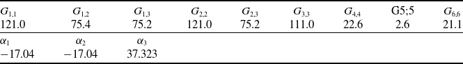
 10×10−9
 K−1
K−1


 Open access