





Introduction
Subglacial topography, the bed elevation beneath the ice, is a controlling factor in ice-sheet evolution. In coastal regions, the advance and retreat of grounding lines are associated with the slope, curvature and elevation of the subglacial bed (Weertman, Reference Weertman1974; Schoof, Reference Schoof2007; Bradwell and others, Reference Bradwell2019; Sergienko and Wingham, Reference Sergienko and Wingham2022). Thus, when modeling ice-sheet evolution, different estimates of subglacial topography can directly affect simulated ice-stream stability (Gasson and others, Reference Gasson, DeConto and Pollard2015; Castleman and others, Reference Castleman, Schlegel, Caron, Larour and Khazendar2022; Wernecke and others, Reference Wernecke, Edwards, Holden, Edwards and Cornford2022). Subglacial topography is also a critical component in multiple englacial and subglacial processes. For example, previous studies have demonstrated how subglacial topography influences basal traction (Bingham and others, Reference Bingham2017; Kyrke-Smith and others, Reference Kyrke-Smith, Gudmundsson and Farrell2018; Hoffman and others, Reference Hoffman, Christianson, Holschuh, Case, Kingslake and Arthern2022), geothermal heat flow (Colgan and others, Reference Colgan2021; Shackleton and others, Reference Shackleton, Matsuoka, Moholdt, van Liefferinge and Paden2023), ice deformation (Meyer and Creyts, Reference Meyer and Creyts2017; Law and others, Reference Law, Christoffersen, MacKie, Cook, Haseloff and Gagliardini2023; Liu and others, Reference Liu, Räss, Herman, Podladchikov and Suckale2024) and subglacial hydrology (Siegert and others, Reference Siegert, Ross and Le Brocq2016; MacKie and others, Reference MacKie, Schroeder, Zuo, Yin and Caers2021b), each of which significantly impacts ice-sheet evolution, and hence the projected sea level rise contributions.
Despite its importance, Antarctic subglacial topography is only sparsely measured. Bed elevation measurements are primarily provided by airborne ice-penetrating radar, which samples data along the aircraft’s flight lines. Densely sampled coastal regions of Antarctica have flight lines separated by 5–20 km, and data gaps in inland Antarctica can easily exceed 50 km (Frémand and others, Reference Frémand2023; Matsuoka and others, Reference Matsuoka2025).
These sparse bed elevation measurements must be interpolated to produce a gridded subglacial topographic map for ice-sheet modeling applications (e.g. Herzfeld and others, Reference Herzfeld, Eriksson and Holmlund1993). The interpolated subglacial topography and resulting ice thickness also need to conserve mass, which is a critical physical constraint for ice-sheet models. However, Seroussi and others (Reference Seroussi2011) showed that traditional interpolation methods, such as kriging, produce subglacial topography that violates the mass conservation constraint when used with observed ice velocity. This violation manifested as spurious, large-magnitude ice flux divergences, which can cause large and rapid changes in ice thickness in the first few numerical model time steps when simulating the glacier evolution.
To find a physically realistic subglacial topography producing realistic ice flow behaviors, several methods have been proposed to invert subglacial topography using physical models or constraints. These methods include numerically solving for subglacial topography from mass conservation (Morlighem and others, Reference Morlighem, Rignot, Seroussi, Larour, Ben Dhia and Aubry2011; McNabb and others, Reference McNabb2012), simultaneously inverting for subglacial topography and basal sliding parameters to reproduce observed ice velocity in ice flow models (e.g. Perego and others, Reference Perego, Price and Stadler2014), inverting for subglacial topography that reproduces the observed surface elevation with a known surface climate forcing (van Pelt and others, Reference van Pelt2013) and adopting machine learning approaches to find an optimal subglacial topography that minimizes ice flux divergences (Teisberg and others, Reference Teisberg, Schroeder and MacKie2021). These methods reconstructed subglacial topographies that show fewer physical artifacts than other methods when combined with observed ice surface elevation or ice velocity, which is valuable for initiating ice flow models. Specifically, the method proposed in Morlighem and others (Reference Morlighem, Rignot, Seroussi, Larour, Ben Dhia and Aubry2011) has been used in BedMachine (Morlighem and others, Reference Morlighem2017; Reference Morlighem2020), a widely-used subglacial topography dataset, to estimate subglacial topography in the fast-flowing regions of the Antarctic and Greenland Ice Sheets.
While the BedMachine estimate of subglacial topography in the fast-flowing region conserves ice mass, this solution to mass conservation has several limitations. First, the topography is often unrealistically smooth. Specifically, Morlighem and others (Reference Morlighem, Rignot, Seroussi, Larour, Ben Dhia and Aubry2011) used mass conservation to solve for an optimized subglacial topography that minimizes the gradients of ice thickness. This topography is not required to reproduce the topographic roughness in the bed elevation measurements (MacKie and others, Reference MacKie, Schroeder, Zuo, Yin and Caers2021b) and is usually much smoother than the observed topography (Hoffman and others, Reference Hoffman, Christianson, Holschuh, Case, Kingslake and Arthern2022). Second, the subglacial topographic uncertainty is not robustly quantified and cannot be easily propagated into ice-sheet models. The topographic uncertainty in Morlighem and others (Reference Morlighem, Rignot, Seroussi, Larour, Ben Dhia and Aubry2011) is presented as maximum error bounds. This uncertainty reflects how heuristically estimated errors in ice velocity, surface and basal mass balance and surface elevation change rate might affect the optimized solution. However, this approach only accounts for the subglacial topography solutions that maximize smoothness. In addition, the error bounds do not represent each possible subglacial topography, and thus cannot be directly used to propagate topographic uncertainty into ice-sheet modeling results.
In contrast to deterministic interpolation approaches, geostatistical simulation methods can generate multiple realizations of subglacial topography with realistic morphology. Geostatistical simulations are methods that interpolate sparse measurements to produce a field of parameters (Deutsch and Journel, Reference Deutsch and Journel1992; Goovaerts, Reference Goovaerts1997). Instead of creating a smooth topography interpolation that maximizes accuracy, like with kriging, geostatistical simulation prioritizes reproducing the spatial variability, or roughness, of the topography (Goff and others, Reference Goff, Powell, Young and Blankenship2014; MacKie and others, Reference MacKie, Schroeder, Caers, Siegfried and Scheidt2020; Neven and others, Reference Neven, Dall’Alba, Juda, Straubhaar and Renard2021). In addition, geostatistical simulation stochastically generates multiple equally probable realizations of the topography, which quantifies uncertainty arising from sparse measurements and allows propagating this uncertainty into glacier models (e.g. Wernecke and others, Reference Wernecke, Edwards, Holden, Edwards and Cornford2022).
Subglacial topography generated by geostatistical simulation has supported scientific discoveries about glacier systems. For example, Zuo and others (Reference Zuo, Yin, Pan, MacKie and Caers2020) and MacKie and others (Reference MacKie, Schroeder, Steinbrügge and Culberg2021a) used geostatistically simulated topography to show that subglacial water routing paths are highly sensitive to topographic uncertainty. In thermodynamic modeling of ice deformation, Law and others (Reference Law, Christoffersen, MacKie, Cook, Haseloff and Gagliardini2023) found that using geostatistically simulated topography led to enhanced ice deformation and a variable-thickness temperate ice layer at the base, which aligned more closely with borehole temperature observations. In contrast, the model with the BedMachine topography produced reduced ice deformation and a thin basal temperate ice layer.
Although traditional geostatistical simulation methods can preserve topographic roughness and quantify uncertainty due to sparse measurements, they do not conserve mass and can consequently introduce physical inconsistencies in ice flux. As a first step in addressing the issue, MacKie and others (Reference MacKie, Schroeder, Zuo, Yin and Caers2021b) employed a co-simulation technique in which topography is geostatistically simulated to correlate with mass-conserving topography from BedMachine (Morlighem and others, Reference Morlighem2017). Although this approach visually aligned topographic realizations more closely with mass conservation constraints, it did not guarantee that ice mass is conserved, as the mass conservation equation is neither explicitly used nor proven to be satisfied in the workflow.
To reconcile the needs of imposing the mass conservation constraint, preserving realistic roughness and estimating topographic uncertainty, we combine geostatistical simulation with mass conservation enforcement to generate subglacial topography realizations. This integration allows geophysical inversion to recover topography that remains realistically rough. Geostatistical inversion has previously been applied in other disciplines, such as petroleum exploration and groundwater hydrology. Geostatistical inversion is typically implemented in a Markov chain Monte Carlo (MCMC) framework, where random subsets of the parameter field are iteratively geostatistically perturbed until a geophysical forward model agrees with observations (Fu and Gómez-Hernández, Reference Fu and Gómez-Hernández2008; Mariethoz and others, Reference Mariethoz, Renard and Caers2010; Shamsipour and others, Reference Shamsipour, Chouteau, Marcotte and Keating2010; Nunes and others, Reference Nunes2012; Volkova and Merkulov, Reference Volkova and Merkulov2019; Reuschen and others, Reference Reuschen, Xu and Nowak2020). In this framework, geostatistical realizations are repeatedly updated and tested against physical constraints, which produces stochastic samples that preserve spatial structure while satisfying governing equations (e.g. Hansen and others, Reference Hansen, Cordua and Mosegaard2012). Once convergence is achieved, additional samples are drawn to form an ensemble that quantifies uncertainty. This strategy is advantageous because it explores the parameter space without requiring a closed-form solution to the inverse problem, making it well-suited for non-unique problems. In this paper, we adopt a similar MCMC approach where subglacial topography is iteratively updated using geostatistical methods, and the update is accepted or rejected based on mass conservation criteria.
In what follows, we first describe the study regions, observational data used and the quality control of bed elevation data. Next, in the Methods section, we outline the workflow, review the key theories and explore the implementation details. In the Results section, we quantitatively present the subglacial topography realizations sampled by the geostatistical MCMC. Finally, in the Discussion section, we discuss the implications of the results and future applications.
Study regions and data
Study regions
We apply our method to the Denman Glacier and Totten Glacier regions where ice velocity exceeds 50  $m \ a^{-1}$ (Fig. 1). Denman and Totten Glaciers are major outlet glaciers in East Antarctica with an annual ice discharge of $\sim$59.2 Gt and $\sim$71.4 Gt from 2009 to 2017, respectively (Rignot and others, Reference Rignot, Mouginot, Scheuchl, van den Broeke, van Wessem MJ and Morlighem2019). Denman Glacier is thought to rest on a steep retrograde bed slope near its current grounding line, making it vulnerable to rapid future retreat (Morlighem and others, Reference Morlighem2020). Specifically, BedMachine estimates the subglacial topography beneath Denman Glacier to be as deep as 3500 m below sea level (Morlighem and others, Reference Morlighem2020). However, the shape and depth of the trough are not well-resolved in ice-penetrating radar, where the radar measurements at the center of the trough do not capture clear return signals from the bed (Liu and others, Reference Liu, Purdon, Stafford, Paden and Li2016; MacGregor and others, Reference MacGregor2021). These potentially erroneous bed elevation measurements of the trough present challenges for inverting for subglacial topography. The second study region, Totten Glacier, is characterized by a large area of high-velocity ice and relatively low large-scale variability in bed elevation measurements. Totten Glacier has extensive grounding line retreat documented in the paleo records (Aitken and others, Reference Aitken2016) and observed in recent decades (Li and others, Reference Li, Rignot, Morlighem, Mouginot and Scheuchl2015; Reference Li, Dawson, Chuter and Bamber2023). Large basal hydrology channels discovered in Totten Glacier could also affect the glacier’s evolution (Dow and others, Reference Dow, McCormack, Young, Greenbaum, Roberts and Blankenship2020; Pelle and others, Reference Pelle, Greenbaum, Ehrenfeucht, Dow and McCormack2024). These two case studies represent subglacial environments with different characteristics, providing diverse test cases for our method.
(a) Antarctic Ice Sheet grounding lines (solid blue lines) (Haran and others, Reference Haran, Klinger, Bohlander, Fahnestock, Painter and Scambos2018) and the zoom-in region in East Antarctica shown in subplot b. (b) Ice surface velocity magnitude (Rignot and others, Reference Rignot, Mouginot and Scheuchl2017) overlaid by contour lines of the surface elevations (Howat and others, Reference Howat, Porter, Smith, Noh and Morin2019) with ice shelf and open ocean region colored as light and deep blue, respectively (Morlighem and others, Reference Morlighem2020).

Figure 1 Long description
The map shows a section of East Antarctica, focusing on the ice surface velocity magnitude. The velocity is represented by a gradient scale from 0 to 500 meters per year. Grounding lines are marked with solid black lines. The map includes labeled regions such as Totten and Denman. The ice shelf areas are marked in light blue, while the ice-free ocean regions are in a deeper blue. The map uses polar stereographic coordinates with Easting (km) and Northing (km) axes. An inset map (a) highlights the study area within Antarctica. The legend indicates the color coding for ice shelf and ocean regions, as well as the grounding line representation.
Data sources
The data used to reconstruct the subglacial topography are presented in Figures 2 and 3. We use MEaSUREs InSAR-Based Antarctica Ice Velocity Map version 2 (Rignot and others, Reference Rignot, Mouginot and Scheuchl2017) for ice surface velocity, which is available at 450 m resolution (Figs. 2b and 3b). We use ice surface elevation in BedMachine v3 at 500 m resolution (Morlighem and others, Reference Morlighem2020), which is inferred from the Reference Elevation Model of Antarctica dataset of ice surface elevation (Howat and others, Reference Howat, Porter, Smith, Noh and Morin2019), corrected for firn-depth (Figs. 2b and 3b). To distinguish between surface topography and subglacial topography, we only refer to surface topography as surface elevation in the following sections. We obtain the classification of regions (grounded ice, floating ice, open ocean, ice-free) from BedMachine at 500 m resolution (Figs. 2c and 3c). We obtain the surface elevation change rate by averaging the elevation change between May 2014 and May 2016 from MEaSUREs ITS_LIVE Antarctic Grounded Ice Sheet Elevation Change version 1 at 1.92 km resolution (Nilsson and others, Reference Nilsson, Gardner and Paolo2023) (Figs. 2d and 3d). We also obtain the surface mass balance by averaging the surface mass balance estimates between 2014 and 2016 from the Regional Atmospheric Climate Model (RACMO2.3p2), which produces outputs at 27 km resolution (van Wessem and others, Reference van Wessem2018) (Figs. 2e and 3e). We fit all data listed above onto a regular grid with 1 km resolution, which is also the grid used for simulating subglacial topography. We use nearest neighbor interpolation for classification of regions, and linear interpolation for all other data.
We compile bed elevation measurements on a 1 km resolution regular grid in polar stereographic coordinates using multiple datasets (Figs. 2a and 3a). In the grounded ice region, we use bed picks from ice-penetrating radar data assembled in Bedmap2 (Fretwell and others, Reference Fretwell2013) and Bedmap3 (Frémand and others, Reference Frémand2023). Each grid cell in the grounded ice region is assigned the average bed elevation from the available radar measurements within that cell. If no measurements are available, the cell remains empty. In the following sections, the grid cells assigned with values are referred to as bed elevation measurements. Several radar campaigns are used in the study region: the NASA Operation IceBridge campaign (MacGregor and others, Reference MacGregor2021), the ICECAP campaign (Young and others, Reference Young2011; Blankenship and others, Reference Blankenship2017), the ICECAP-EAGLE campaign (Young and others, Reference Young, Schroeder, Blankenship, Kempf and Quartini2016; Roberts and others, Reference Roberts2023), the ICECAP-OLDICE campaign (Young and others, Reference Young, Schroeder, Blankenship, Kempf and Quartini2016), the Talos-Dome campaign in 2003 (Bianchi and others, Reference Bianchi2003) and the Stanford-Cambridge Radar Film Digitization Project (Schroeder and others, Reference Schroeder2019).
For regions classified as ice-free ocean, floating ice and ice-free land, we project the BedMachine v3 bed elevation (Morlighem and others, Reference Morlighem2020) from its 500 m grid to our 1 km grid using linear interpolation. Bedmap2 and Bedmap3 data are converted from EIGEN-GL04C geoid (Förste and others, Reference Förste2008) to EIGEN-6C4 geoid (Förste and others, Reference Förste2014) used in BedMachine to ensure consistency between different datasets.
Processed datasets used for inverting for subglacial topography at Denman Glacier. The dashed gray line delineates regions with ice surface velocity magnitude greater than 50  $m \ a^{-1}$. The solid black line represents grounding lines traced based on BedMachine region classification (Morlighem and others, Reference Morlighem2020). Subplot a shows gridded bed elevation measurements in Denman Glacier before the quality control step (Fretwell and others, Reference Fretwell2013; Morlighem and others, Reference Morlighem2020; Frémand and others, Reference Frémand2023), where ice-free land, ice-shelf and ice-free ocean regions have BedMachine subglacial topography/bathymetry. Subplot b plots ice surface velocity magnitude (Rignot and others, Reference Rignot, Mouginot and Scheuchl2017) overlaid by the contour lines of the surface elevation (Howat and others, Reference Howat, Porter, Smith, Noh and Morin2019; Morlighem and others, Reference Morlighem2020); c shows the classification of regions obtained from BedMachine (Morlighem and others, Reference Morlighem2020); d shows surface elevation change rate (Nilsson and others, Reference Nilsson, Gardner and Paolo2023); e shows the interpolated surface mass balance overlaid by the original surface mass balance estimations (van Wessem and others, Reference van Wessem2018) marked in black-edge circles.

Figure 2 Long description
A set of five thematic maps of Denman Glacier in East Antarctica. A) The bed elevation map shows elevation in meters, ranging from -2000 to 2000, with colored tracks indicating measurement paths. The dashed line marks high-velocity regions and the solid line indicates grounding lines. B) The ice surface velocity map displays velocity in meters per year, ranging from 0 to 800, with contour lines representing surface elevation. Fast flow is concentrated near the outlet and ice shelf. C) The classification map identifies grounded ice, ice-free land and ice-shelf areas, with black contour lines marking boundaries. D) The surface elevation change rate map shows changes in meters per year, ranging from -1 to 1, indicating thinning and thickening patterns. E) The surface mass balance map presents mass balance in meters of ice equivalent per year, ranging from 0.25 to 1.00, with higher values near the coast. Black-edge circles mark original estimations. The maps are oriented with polar steoreographic coordinates, providing a comprehensive view of the glacier's dynamics and changes.
Processed dataset used for inverting subglacial topography of Totten Glacier, similar to Figure 2. The dashed gray line delineates regions with ice surface velocity magnitude greater than 50  $m \ a^{-1}$. The solid black line represents grounding lines traced based on BedMachine region classification (Morlighem and others, Reference Morlighem2020). Subplot a shows gridded bed elevation measurements before the quality control step (Fretwell and others, Reference Fretwell2013; Morlighem and others, Reference Morlighem2020; Frémand and others, Reference Frémand2023), where ice-free land, ice-shelf and ice-free ocean regions are colored by BedMachine subglacial topography/bathymetry. Subplot b plots ice surface velocity magnitude (Rignot and others, Reference Rignot, Mouginot and Scheuchl2017) overlaid by contour lines of the surface elevation (Howat and others, Reference Howat, Porter, Smith, Noh and Morin2019); c shows the classification of regions obtained from BedMachine (Morlighem and others, Reference Morlighem2020); d shows surface elevation change rate (Nilsson and others, Reference Nilsson, Gardner and Paolo2023); e shows interpolated surface mass balance map overlaid by the original surface mass balance estimations (van Wessem and others, Reference van Wessem2018) marked in black-edge circles.

Figure 3 Long description
Five thematic maps of Totten Glacier in East Antarctica are presented. The maps use polar stereographic coordinates in kilometers. The first map shows bed elevation measurements with a dashed line for high-velocity regions and a solid line for grounding lines. The second map displays ice surface velocity magnitude with a scale from 0 to 500 meters per year, overlaid with contour lines for surface elevation. The third map classifies regions into grounded ice, ice-shelf, ice-free land and ice-free ocean. The fourth map illustrates surface elevation change rate, ranging from -1 to 1 meters per year. The fifth map shows surface mass balance, ranging from 0 to 2 meters of ice equivalent per year, with original estimations marked by black-edge circles. High velocities are concentrated near the grounding line, while elevation changes are more negative near the coast when compared to inland.
Data quality control
We perform quality control on bed elevation data to identify and remove potentially erroneous measurements. Bed elevation measurements could be affected by instrumental errors, radio-wave velocity errors, bed-picking errors, GPS errors and clutter (Lapazaran and others, Reference Lapazaran, Otero, Martín-Español and Navarro2016). Clutter occurs when radar echoes are reflected from off-nadir topographic high points, which often happens on high-relief subglacial topography such as deep troughs. Compared to other sources of positive or negative errors, radar clutter can cause the returned bed elevation to have a large-magnitude positive bias (Lapazaran and others, Reference Lapazaran, Otero, Martín-Español and Navarro2016; Scanlan and others, Reference Scanlan, Rutishauser, Young and Blankenship2020).
Radar errors complicate bed mapping efforts. Often, the quality control of bed elevation data is performed by visual inspection or by comparison with other data sources at a few cross-over locations (e.g. Farinotti and others, Reference Farinotti, King, Albrecht, Huss and Gudmundsson2014; Lippl and others, Reference Lippl, Blindow, Fürst, Marinsek, Seehaus and Braun2020), which lacks a quantitative assessment. In this paper, we implement an MCMC quality control procedure. We first exclude bed elevation measurements that are greater than or equal to ice surface elevation. Then, we perform a Metropolis–Hastings MCMC analysis (Metropolis and others, Reference Metropolis, Rosenbluth, Rosenbluth, Teller and Teller1953; Hastings, Reference Hastings1970), which perturbs the subglacial topography using spatially-correlated noise and accepts or rejects realizations based on penalties for ice flux divergences and misfits from bed elevation measurements. This analysis provides subglacial topography realizations that reduce spurious ice flux divergences while maintaining differences to bed elevation measurements comparable to those in BedMachine, allowing us to identify and exclude measurements that cannot be reconciled with a mass-conserving topography. To address the potentially large-magnitude radar errors, e.g. from radar clutter and other erroneous measurements, we remove bed elevation measurements that are 1.5 standard deviations shallower than the generated subglacial topography realizations. The full details of the data quality control step are documented in the Supplementary Material sections 1 and 2.
For the Denman region, we also remove bed elevation measurements in 10 additional grid cells on a radar flight line near the narrowed trunk of the glacier, where a subglacial trough likely exists and could potentially cause significant bed elevation errors (Forte and others, Reference Forte, Bondini, Bortoletto, Dossi and Colucci2019). For the Totten region, we remove additional bed elevation measurements from one radar flight line whose cross-over errors exceed 1000 m when compared with nearby flight lines. These additional bed elevation measurements are also not used in BedMachine topography (Morlighem and others, Reference Morlighem2020).
In total, we removed  $1.45\%$ and $2.2\%$ of bed elevation measurements in the Denman and Totten regions of high-velocity ice, respectively. For context, we compared the removed bed elevation measurements to BedMachine (Morlighem and others, Reference Morlighem2020) and BedMap gridded subglacial topography (Pritchard and others, Reference Pritchard2025). For Denman Glacier, the averaged absolute difference between removed bed elevation measurements and BedMachine is 2356 m, while the difference with Bedmap is 1829 m. For Totten Glacier, the same comparisons yield differences of 667 m and 595 m, respectively.
Methods
Overview
We present an MCMC approach to generating subglacial topography realizations in regions with high-velocity ice, such that the realizations conserve ice mass, honor bed elevation measurements and have realistic roughness. The MCMC algorithm iteratively proposes new topography and evaluates the proposed topography by mass conservation. We design two steps to generate topography realizations, where each step constructs Markov chains with a distinct proposal method and creates topographic features of different spatial scales (Fig. 4). In the first step, we generate large-scale topographic features (lateral dimension  $ \gt $ 10 km) that improve the consistency with mass conservation (Fig. 4a). We run Markov chains, which we refer to as large-scale chains, that iteratively propose new topography by adding blocks of positive and negative perturbations to the previous topography. These large-scale chains generate subglacial topographies that preserve the bed elevation measurements, but they do not guarantee realistic topographic roughness. In the second step, we update topography sampled from large-scale chains to honor the spatial roughness of subglacial topography (Fig. 4b). In this step, we run a second set of Markov chains, which we refer to as small-scale chains, that propose new topography by replacing small-scale features (lateral dimension $\leq$ 10 km). These new features are generated by Sequential Gaussian Simulation, a geostatistical interpolation method that honors the spatial roughness of the simulated topography. The final topography ensemble consists of the topography produced in each small-scale chain, which captures diverse topographic features with realistic roughness while maintaining low mass conservation misfits.
In the following subsections, we first summarize key concepts in geostatistics, mass conservation and MCMC to discuss how they are adapted for simulating subglacial topography. Then we describe the implementation details of the large-scale chain and small-scale chains. At the end, we outline how these chains are combined to generate the topography ensemble.
A simplified schematic diagram for using the large-scale and small-scale chains to generate subglacial topographies. We present subglacial topographies as 1D lines for simplification. Subplot a represents the large-scale chains, where new subglacial topography (blue lines) is proposed by adding random perturbations (gray line in step 3). Subplot b represents the small-scale chains, where the small-scale features in the topography are replaced by simulations generated by SGS (orange lines).

Figure 4 Long description
The diagram consists of two main sections: a. Large-Scale Chain and b. Small-Scale Chain. In the Large-Scale Chain section: 1. Geostatistically simulate subglacial topography using bed elevation measurements. 2. Compute mass flux residuals using the topography. 3. Add random perturbation with zero change at measurements. 4. Re-compute mass flux residuals. 5. Accept or reject changes from step 3 based on the mass flux residuals. 6. Repeat steps 3-5 until convergence, then continue generating new samples to produce an ensemble. Output: Ensemble of large-scale simulations with reduced mass flux residuals. Use large-scale ensemble to initialize small-scale ensemble. In the Small-Scale Chain section: 1. Initialize with outputs from the large-scale chain. 2. Compute mass flux residuals using the topography. 3. Resimulate small-scale features using Sequential Gaussian Simulation. 4. Re-compute mass flux residuals. 5. Accept or reject changes from step 3 based on the mass flux residuals. 6. Repeat steps 3-5 until convergence, then obtain one topography realization for each chain. Output: Ensemble of small-scale simulations with minimized mass flux residuals. These realizations are realistically rough.
Geostatistics: the bed elevation constraint
Observations of subglacial topography provide direct elevation constraints and information on the spatial correlation of topographic features. The latter is visually expressed as the topography’s roughness and can be quantified by semi-variogram statistics (e.g. MacKie and others, Reference MacKie, Schroeder, Zuo, Yin and Caers2021b). The semi-variogram, often referred to simply as the variogram, summarizes the spatial statistics observed in the sparse bed elevation measurements. It describes the two-point correlation structure by relating the lag distance (separation distance) between two elevation measurements to their value differences (Zimmermann and others, Reference Zimmermann, Zehe, Hartmann and Elsenbeer2008):
 \begin{equation}
\gamma(h) = \frac{1}{2N(h)} \sum_{i = 1}^{N(h)} (T(x_i) - T(x_i + h))^2.
\end{equation}
\begin{equation}
\gamma(h) = \frac{1}{2N(h)} \sum_{i = 1}^{N(h)} (T(x_i) - T(x_i + h))^2.
\end{equation} In Equation 1,  $h$ is the lag distance. $T(x_i)$ is the bed elevation at the location $x_i$. $x_i+h$ represent locations that are $h$ away from $x_i$. $N(h)$ is the number of data pairs separated by distance $h$. Intuitively, when two grid cells on the topography map are farther away (a larger $h$), their elevations become less correlated (a larger $\gamma(h)$) until the correlation vanishes and $\gamma(h)$ levels off. This produces a typical variogram shape where $\gamma(h)$ increases with $h$ until it reaches a plateau. The empirical variogram calculated from sparse measurements can be fitted into a variogram model, defined by the variogram model type (Gaussian, Spherical, Exponential or Matern). The variogram model is described by the range (maximum $\gamma(h)$), sill (h at which $\gamma(h)$ reaches maximum) and nugget ( $\gamma(0)$) parameters. A smaller range or a larger sill could indicate large variability of subglacial topography over a short spatial distance, and vice versa. The variogram model can be used for comparing the spatial roughness of different subglacial topographies and for generating topography with realistic roughness (MacKie and others, Reference MacKie, Schroeder, Zuo, Yin and Caers2021b). In this paper, we use functions in the SciKit-Gstats Python package with the Cressie estimator to compute experimental variograms and fit variogram models (Mälicke, Reference Mälicke2022).
While kriging interpolation uses the variogram to provide a single deterministic estimate of the bed, Sequential Gaussian Simulation (SGS) generates multiple realizations of subglacial topography that honor sparse bed elevation measurements while reproducing the variogram statistics (MacKie and others, Reference MacKie, Schroeder, Zuo, Yin and Caers2021b). SGS is a geostatistical conditional simulation method that stochastically interpolates sparse measurements to produce equally probable realizations of a random field. SGS is a ‘conditional’ simulation method because the generated realizations exactly match available measurements. SGS has been shown to be effective in stochastically generating subglacial topography in regions with slow ice flow (e.g. MacKie and others, Reference MacKie, Schroeder, Caers, Siegfried and Scheidt2020; Law and others, Reference Law, Christoffersen, MacKie, Cook, Haseloff and Gagliardini2023); but when it is used for regions with fast ice flow, the simulated subglacial topography is often incompatible with mass conservation. Additionally, in some regions with high-relief topographic features, incomplete radar sampling may limit the range of bed elevations represented in SGS realizations. For example, in the Denman region, BedMachine (Morlighem and others, Reference Morlighem2020) and Bedmap3 (Pritchard and others, Reference Pritchard2025) resolve a deep subglacial trough reaching elevations of -3700 m and -2800 m, respectively, whereas the bed elevation measurements within 50 km of the trough only reach -2200 m. In cases where the true bed elevation in large data gaps differs greatly from the surrounding topography, the Gaussian nature of SGS makes its realizations unlikely to reproduce prominent features with elevations that extend beyond the range of measurements (Supplementary Material section 6). This limitation means that SGS alone is insufficient for sampling subglacial topography in regions with extreme relief.
To address this limitation, we adapt geostatistical simulation for mass-conserving topographies by dividing the process into two stages: (1) generating the large topographic features in the large-scale chains, and (2) re-simulating finer features constrained by the variogram statistics in the small-scale chains. We use SGS implemented in MacKie and others (Reference MacKie2023) to generate topography in regions with low-velocity ice, to initiate the large-scale chains and to simulate realistically rough topographies in the small-scale chains.
Mass conservation: the physical constraint
Mass conservation provides valuable information to ensure the compatibility of simulated topographies with other ice surface observations, such as ice surface velocity, surface mass balance and surface elevation change rate (Seroussi and others, Reference Seroussi2011). The mass conservation equation (2) is derived by depth-integrating the ice continuity equation under the assumption of incompressible ice. The equation relates the sparsely measured subglacial topography with high-resolution ice velocity.
 \begin{equation}
\frac{\partial H}{\partial t} = - \nabla \cdot ({\bar{u}} H) + \dot M_s + \dot M_b.
\end{equation}
\begin{equation}
\frac{\partial H}{\partial t} = - \nabla \cdot ({\bar{u}} H) + \dot M_s + \dot M_b.
\end{equation} Here,  $\frac{\partial H}{\partial t}$ is the rate of change of ice thickness, $H$;
$H$;  $\nabla \cdot (\bar{u}H)$ is the depth-integrated ice flux divergence, which calculates the volume of ice entering and leaving a column with depth-averaged velocity, $\bar{u}$. Surface processes, such as surface accumulation (positive) and surface ablation (negative), are represented by the surface mass balance, $\dot M_s$; whereas the basal mass balance, $\dot M_b$, includes basal accumulation (positive) and basal ablation (negative).
We make further adjustments to adapt this universal equation to the available data in the study region. The ice thickness is expressed as the difference between ice surface elevation ( $S$) and bed elevation ( $T$). The annual change in bed elevation is usually orders of magnitude smaller than the change in surface elevation; therefore, we assume $\frac{\partial H}{\partial t} = \frac{\partial (S - T)}{\partial t} \approx \frac{\partial S}{\partial t}$. As annual basal mass balance is estimated to be in centimeter-scale or smaller in the grounded ice region (e.g. Seroussi and others, Reference Seroussi2019; McArthur and others, Reference McArthur, McCormack and Dow2023), we approximate $\dot M_b$ as 0. Additionally, the depth-averaged velocity, $\bar{u}$, is approximated by surface velocity, $u_s$, which is a reasonable assumption in the high-velocity regions where basal sliding dominates (Rignot and others, Reference Rignot, Mouginot and Scheuchl2011; Seroussi and others, Reference Seroussi2011).
Since mass conservation is most effective in high-velocity regions, we first define an inversion domain where our method can be applied. Assuming  $u_s \approx\bar{u}$, we identify grounded ice regions with surface speed $\geq$ 50 $m \ a^{-1}$, which is the threshold for mass-conservation-based topography inversion in BedMachine (Morlighem and others, Reference Morlighem2020). Higher-order ice stream models also showed that surface speed is mostly $ \lt 4\%$ higher than depth-averaged speed in this velocity regime (Morlighem and others, Reference Morlighem, Rignot, Mouginot, Seroussi and Larour2014). We compute a mask of the region, smooth its boundary using a 15-cell mode filter and then expand the mask outward by 3 km. Grid cells classified as open ocean, floating ice and ice-free land are excluded from the region. This region (shown in Figs. 2 and 3), referred to hereafter as the high-velocity region, defines the domain where we apply the MCMC algorithm. Outside the high-velocity region, topography realizations are generated directly using SGS (e.g. MacKie and others, Reference MacKie2023).
After the adjustments, the mass flux residuals, which represent the ice flux divergence unresolved in the mass conservation equation, are defined as:
 \begin{equation}
r = \nabla \cdot (u_s (S-T)) + \frac{\partial S}{\partial t} - \dot M_s.
\end{equation}
\begin{equation}
r = \nabla \cdot (u_s (S-T)) + \frac{\partial S}{\partial t} - \dot M_s.
\end{equation} The mass flux residuals are calculated for each grid cell in the high-velocity region. Spatial derivatives, such as  $\nabla$, are computed using second-order central differences. For simplicity, the spatial discretization notation to represent $r$ at each grid cell $(i,j)$ (e.g. $r_{ij}$) is omitted in this and the following equations, similarly for $S$,
$S$,  $T$,
$T$,  $\frac{\delta S}{\delta t}$ and $\dot M_s$.
Bayes’ theorem and MCMC: combining bed elevation measurements and mass conservation
Mass conservation provides a powerful physical constraint on subglacial topography, but by itself it cannot uniquely resolve the topography. To overcome this limitation, we combine mass conservation with bed elevation measurements in a Bayesian framework. Bayes’ theorem offers a convenient framework to combine these complementary sources of information into a posterior distribution of subglacial topography. Bed elevation measurements, such as the measured values and topographic roughness, define the prior distribution,  $p(T)$. The spurious ice fluxes due to violations of mass conservation describe the likelihood function of the subglacial topography, $p(d|T)$, where $d$ contains $\lbrack S,u_s,\frac{\delta S}{\delta t},{\dot M}_s\rbrack$. Combining the prior and likelihood yields the posterior distribution of subglacial topography according to Bayes’ theorem:
 \begin{equation}
p(T|d) = \frac{p(d|T) p(T)}{p(d)}.
\end{equation}
\begin{equation}
p(T|d) = \frac{p(d|T) p(T)}{p(d)}.
\end{equation} Because the posterior distribution defined by Bayes’ theorem cannot be obtained analytically, we use MCMC to approximate it. MCMC is a well-established sampling method that generates a sequence of samples (a Markov chain) from complex distributions (Gallagher and others, Reference Gallagher, Charvin, Nielsen, Sambridge and Stephenson2009; Geyer, Reference Geyer2011). At each iteration, MCMC proposes a perturbation to the current realization of the parameter field, creating a new candidate. This new candidate is then evaluated against the prior and the physical constraint using the likelihood function. This evaluation determines whether the new candidate is accepted or rejected. Typically, the chain runs for many iterations until convergence, after which subsequent realizations are used to approximate the posterior. In our application, the Markov chain is composed of a sequence of subglacial topography realizations  $T_i$ with $i \in {0,1,2,3...}$.
There are many different MCMC sampling algorithms. We use the widely used Metropolis–Hastings (MH) approach (Metropolis and others, Reference Metropolis, Rosenbluth, Rosenbluth, Teller and Teller1953; Hastings, Reference Hastings1970), which efficiently balances optimization with exploration of the parameter space and is known for its simple and flexible implementation. In this framework, candidate topographies that reduce misfit (i.e. lower mass flux residuals) are accepted, while those that increase misfit can still be accepted with some probability, which is determined by the posterior distribution. This strategy prevents the chain from becoming trapped in local solutions, enabling the exploration of plausible subglacial topographies. Starting from an initial guess of subglacial topography  $T_0$, each $T_i$ is iteratively generated for $i$ as described below.
(1) propose a new realization $T'$ by updating
$T_i$
$T'$ by updating
$T_i$denote the probability of obtaining
$T'$ from
$T_i$ as
$q(T'|T_i)$(2) compute posterior distribution of
$T'$:
$p(T'|d) = \frac{p(d|T')p(T')}{p(d)}$compute posterior distribution of
$T_i$:
$p(T_i|d) = \frac{p(d|T_i)p(T_i)}{p(d)}$(3) compute acceptance probability
$\alpha(T',T_i) = \min \left[ \frac{p(d|T')p(T')q(T_i| T')}{p(d|T_i)p(T_i)q(T'|T_i)}, 1\right] $(4) with probability
$\alpha(T',T_i)$, accept
$T'$ and let
$T_{i+1}$ be
$T'$with probability
$1-\alpha(T',T_i)$, let
$T_{i+1}$ be
$T_i$





The proposal step in the MCMC algorithm searches through the space of possible subglacial topographies, while the acceptance probability  $\alpha$ governs which candidate topography samples are retained.
In our method, we adopt a special case of the MH algorithm, called the Extended Metropolis algorithm (Mosegaard and Tarantola, Reference Mosegaard and Tarantola1995). The key difference is that, rather than explicitly evaluating the prior  $p(T)$, Extended Metropolis directly generates proposed topography from the prior distribution. In other words, the proposal distribution equilibrates to the prior distribution such that
 \begin{equation}
\frac{q(T_i|T')}{q(T'|T_i)} = \frac{p(T_i)}{p(T')},
\end{equation}
\begin{equation}
\frac{q(T_i|T')}{q(T'|T_i)} = \frac{p(T_i)}{p(T')},
\end{equation}and the acceptance probability of  $T'$ given $T_i$, $\alpha(T',T_i)$, is simplified to a comparison of likelihoods:
 \begin{equation}
\alpha(T',T_i) = \min \left[ \frac{p(d|T')}{p(d|T_i)}, 1 \right].
\end{equation}
\begin{equation}
\alpha(T',T_i) = \min \left[ \frac{p(d|T')}{p(d|T_i)}, 1 \right].
\end{equation} The Extended Metropolis algorithm is particularly well-suited to our problem because the prior distribution of subglacial topography can be efficiently represented by geostatistical simulations. In this framework, candidate realizations are drawn directly from the geostatistical prior, which ensures that the proposals already satisfy the geostatistical properties of the bed while the acceptance step enforces consistency with mass conservation. A similar approach was applied in Hansen and others (Reference Hansen, Cordua and Mosegaard2012), where geostatistical priors were used to generate proposals directly from simulation. We utilize different proposal methods in the large-scale chain and the small-scale chain to update the topography, and we explain their associated priors in the later sections. The likelihood function is represented by  $p(d|T)$, where $d$ contains $S,u_s,\frac{\delta S}{\delta t},{\dot M}_s$. We define $p(d|T)$ in terms of the spurious mass flux residuals $r$ for a given topography $T$.
$T$.
Ideally, the mass flux residuals  $r$ should be zero upon convergence, but in practice, uncertainties in ice velocity, surface mass balance and surface elevation change rate introduce nonzero values of $r$. To account for these potential uncertainties, we define $r$ at every grid cell to be an independent Gaussian distribution with standard deviation $\sigma_r$, as shown below.
 \begin{equation}
p(d|T) = \exp{\left( - \frac{\sum(r^2)}{2\sigma_r^2} \right).}
\end{equation}
\begin{equation}
p(d|T) = \exp{\left( - \frac{\sum(r^2)}{2\sigma_r^2} \right).}
\end{equation} We use BedMachine as a baseline mass-conserving topography to calibrate  $\sigma_r$ and test our method’s ability to reduce mass flux residuals. Specifically, we approximate the distribution of $r$ by fitting a Gaussian distribution to the mass flux residuals from the BedMachine topography in the high-velocity region, yielding $\sigma_r \approx 3.5 \ m \ a^{-1}$ at Denman Glacier and $\sigma_r \approx 4.5 \ m\ a^{-1}$ at Totten Glacier. While this calibration is not fully independent—since BedMachine is also used as a benchmark—we note that $\sigma_r$ functions primarily as a scaling parameter in the likelihood. Its role is to control how strongly mass flux residuals are penalized, rather than to bias inference toward BedMachine and our results are not sensitive to modest changes in its value. In Supplementary Material section 3, we further evaluate $r$ in regions with dense subglacial measurements to confirm that the Gaussian distribution estimated from BedMachine falls within the plausible range of residual values. Ideally, $\sigma_r$ would be derived from uncertainties in ice velocity, surface mass balance and surface elevation change rate, but in practice this would be difficult to implement consistently. Other possible approaches for defining the distribution of mass flux residuals based on data uncertainties are discussed in the Discussion section.
Large-scale chain: reconstruct large geometries
As discussed in the Geostatistics section, the Gaussian nature of SGS means that SGS may overlook large features such as deep troughs. As such, we use a two-step MCMC geostatistical inversion procedure that resolves both the large- and small-scale features (Fig. 4). In the first step, we construct Markov chains to resolve large-scale subglacial topographic features (lateral dimensions  $ \gt $ 10 km) that reduce the mass flux residuals.
The large-scale chains search for topographies that satisfy both mass conservation and direct bed elevation measurements, without imposing restrictions on topographic roughness. We start each large-scale chain with an initial guess of the subglacial topography individually generated by SGS (Fig. 4a, step 1). We use SGS-generated initial topography because it provides an estimate of subglacial topography consistent with bed elevation measurements. Then, we iteratively perturb the topography (Fig. 4a, step 3) by adding blocks of Weighted Random Fields (WRF). WRFs are spatially correlated random fields set to zero at the locations of bed elevation measurements, which ensures that observations are preserved while allowing smooth perturbations elsewhere. Because roughness is not enforced, this prior is relatively uninformative, which enables MCMC to capture high-relief features such as troughs when required to conserve mass. We improve convergence efficiency by perturbing only one block of topography per iteration (e.g. Roberts and Sahu, Reference Roberts and Sahu2002). Updating the entire domain often results in favorable changes in one region being canceled by unfavorable changes in others, which lowers acceptance rates. In contrast, block-based updates effectively increase acceptance rates and accelerate convergence. The blocks selected throughout the MCMC algorithm could repeat and overlap, and the subglacial topography at each grid cell is perturbed more than once.
The block perturbation process is illustrated in Figure 5. At each iteration, a random block is chosen within the high-velocity region (Fig. 5, step 3.1), with lateral dimensions drawn from a uniform distribution between 20 and 100 km for Denman Glacier and between 50 and 200 km for Totten Glacier. These block sizes ensure the acceptance rates to remain between 0.1 and 0.4, which usually indicates an efficient MCMC algorithm (Gelman and others, Reference Gelman, Gilks and Roberts1997; Geyer, Reference Geyer2011). Second, a random field with the same size as the block is generated (Fig. 5, step 3.2). The random field is sampled from a multivariate Gaussian distribution with zero mean and an exponential, isotropic covariance model, which allows us to efficiently generate the field using Fourier Transforms implemented in the Python package GSTools (Müller and others, Reference Müller, Schüler, Zech and Heße2022). This covariance model can be represented by a variogram with zero nugget and a range sampled between 10 and 45 km uniformly for the study of Denman Glacier. The maximum range (45 km) represents the variogram range calculated from bed elevation measurements inside the high-velocity region of Denman Glacier, and the minimum range helps to create perturbations that resemble relatively smaller topographic features. With a similar process, the covariance model is chosen to have a variogram range sampled between 10 and 80 km for the Totten Glacier. The amplitude of the random field is sampled from a uniform distribution between 50 and 200 m for Denman and between 100 and 300 m for Totten, which we tuned to keep acceptance rates between 0.1 and 0.4. We then multiply the random field with the weight matrices to force values to taper smoothly to zero at locations with bed elevation measurements and block edges (Fig. 5, step 3.2; also see Supplementary Material section 4). Finally, we add the WRF to the topography inside the block (Fig. 5, step 3.3). Outside the high-velocity region, the topography is masked out and remains unchanged.
The figure expands on step 3 in Figure 4a to illustrate the proposal method used in the large-scale chain. The red rectangle in steps 3.1 and 3.3 represents the selected random block.

Figure 5 Long description
The diagram illustrates the block perturbation process in three steps. On the left, step 3.1 shows a map labeled 'before perturbation' with a red rectangle indicating the block's size and location. The map includes radar flightlines and axes labeled 'X' and 'Y' in kilometers. In the center, step 3.2 details the calculation of the Weighted Random Field (WRF) by multiplying a random field with data weight and block weight. This section includes four images: the Weighted Random Field, Random Field, Data Weight and Block Weight, with color scales for the random fields and weights. The Random Field is labeled with perturbation in meters, while Data Weight and Block Weight are labeled with weight values. The Weighted Random Field is equal to the result of multiplying Random Field, Data Weight, and Block Wieght. On the Weighted Random Field, an arrow points to a location where perturbation is zero, and a note states 'do not perturb bed elevation measurements and merge with outside.' On the right, step 3.3 shows a map labeled 'after perturbation' with the red rectangle indicating the WRF block added to the topography. The map includes a color scale for bed elevation in meters.
Like other MCMC applications, our method requires an initialization period, or burn-in, during which the chain iteratively updates the initial guess before reaching a stationary distribution (i.e. iterations after which the topography realizations are mass-conserving). Thus, we discard the early iterations where the large-scale features have not yet converged to a stationary distribution. We use a trace plot (Figs. S4 and S5) to determine how many iterations to discard (Supplementary Material section 5).
The subglacial topography samples generated in the large-scale chain after burn-in are used to find the topographic trend and serve as initial guesses for the small-scale chains. After the burn-in phase, we calculate the topographic trend,  $T_{trend}$, by taking a topography sample from each large-scale chain and applying a Gaussian smoothing filter with a standard deviation of 5 km. Then we sample 10 topography realizations from each of the 4 large-scale chains to initialize the small-scale chains. Because consecutive iterations in a Markov chain are correlated, we only sample at every k-th iteration to ensure approximate independence between sampled subglacial topographies. This method, called thinning in MCMC literature, is often used to reduce autocorrelation between samples (Jones and Qin, Reference Jones and Qin2022). The value of k is determined by calculating the autocorrelation of topography across iterations (Figs. S6 and S7), which is 4000 iterations for Denman Glacier and 30000 iterations for Totten Glacier (e.g. Mosegaard and Tarantola, Reference Mosegaard and Tarantola1995). Together, each large-scale chain provides a $T_{trend}$ and 10 realizations, $T_{samples}$, which are used to initialize 10 small-scale chains.
Small-scale chain: simulate finer features
Following the large-scale chain, the small-scale chain uses SGS to re-simulate small-scale features (lateral dimension  $\leq$ 10 km) that are not captured by the large-scale trend. Similar to Hansen and others (Reference Hansen, Cordua and Mosegaard2012), each proposal consists of simulating a sub-region of the topography with SGS (Figs. 4b and 6). In this way, small-scale features in the initial topography are iteratively replaced with SGS-generated realizations, which preserve realistic roughness. The SGS proposes updates that are constrained by both bed elevation measurements and topographic roughness, enforcing a geostatistical prior on the subglacial topography. Because these updates are still subjected to the MCMC acceptance criterion, the simulated features remain constrained by the likelihood from mass conservation, as in the large-scale chains.
We initialize the small-scale chains with the topographic trend obtained from the large-scale chain. We first remove large topographic features by subtracting  $T_{trend}$ from $T_{sample}$ (a.k.a. de-trending). Then, we use a normal score transformation (Chilès and Delfiner, Reference Chilès and Delfiner2012) to normalize the de-trended topography. Finally, we also de-trend and normalize the bed elevation measurements and calculate the variogram to represent topographic roughness. The topographic trend $T_{trend}$ is stored and will be added back to simulated de-trended subglacial topography later in the MCMC algorithm.
Equipped with the variogram, the SGS-simulated topographies can reproduce the realistic topographic roughness observed in the bed elevation measurements. In each iteration of the small-scale chain, the re-simulation with SGS is restricted to a random rectangular block (e.g. Fu and Gómez-Hernández, Reference Fu and Gómez-Hernández2008; Hansen and others, Reference Hansen, Cordua and Mosegaard2012; Laloy and others, Reference Laloy, Linde, Jacques and Mariethoz2016) to facilitate the convergence and to satisfy the interdependency requirement of MCMC. In each MCMC iteration, we select the block’s center at a random location within the high-velocity region and sample the block’s lateral dimensions from a uniform distribution between 2 km and 8 km (Fig. 6, step 3.1), which we tuned to achieve acceptance rates between 0.1 and 0.4. Inside the block, we re-simulate grid cells that are not bed elevation measurements (Fig. 6, steps 3.2 and 3.3). The simulation is conditioned on bed elevation measurements inside the block and neighboring subglacial topography outside the block. We then de-normalize the simulation and add back the trend to recover bed elevation, which is then used to calculate the mass-flux residuals and the acceptance probability.
The figure expands on the step 3 in Figure 4b. An illustration of the update method used in the small-scale chain. The red rectangle represents the selected random block.

Figure 6 Long description
The process consists of three steps: Step 3.1 involves randomly choosing the block's size and location, shown with a red rectangle on a map with radar flightlines. Step 3.2 removes grid cells inside the block that are not bed elevation measurements, highlighted within the red rectangle. Step 3.3 re-simulates the removed grid cells using Sequential Gaussian Simulation, again within the red rectangle. The map includes a color scale for bed elevation in meters, ranging from -2000 to 1000.
The subglacial topography outside the high-velocity region is not masked out in the block-based SGS simulations. Because of the block’s small size and its central location within the high-velocity region, it only changes grid cells within approximately 4–5 km of the high-velocity region. This design effectively created a ‘buffer’ zone such that the mass flux residuals are efficiently minimized at the margin of the high-velocity region and the topography merges smoothly with the low-velocity region. The calculation of mass flux residuals, however, is still restricted to within the high-velocity region.
Generate the topography ensemble
While the two-phase perturbation strategy deviates from traditional MCMC implementations, the algorithm retains the fundamental structure of a Bayesian inversion. The geostatistical prior defines plausible spatial correlations, and the physical model acts as a constraint via the likelihood. We explore the posterior through repeated perturbation and acceptance/rejection steps based on the mass flux residuals.
We designed a combination of large-scale and small-scale chains to generate the final ensemble of topography realizations. First, for Denman Glacier, we initiate 4 large-scale chains with different initial topographies, which are simulated using SGS conditioned on the quality-controlled bed elevation measurements (Fig. 4a, step 1). For the Totten Glacier, we initialize 2 large-scale chains with the same process. We reduce the number of large-scale chains for Totten Glacier due to its larger domain and subsequently longer algorithm runtime. After the large-scale topographic features stabilize, we smooth the mean topography of the large-scale chain to obtain the topographic trend. We also sample 10 subglacial topography realizations from each large-scale chain to be used as the initial topography to start the small-scale chains. Next, we run 10 small-scale chains with detrended, normalized subglacial topography. Each small-scale chain runs until  $\sim$80 $\%$ of the grid cells inside the high-velocity region have been updated at least once. One topography realization is sampled at the end of each small-scale chain. In total, Denman Glacier has 4 large-scale chains that diverge into 40 small-scale chains, which provide an ensemble of 40 topography realizations. Totten Glacier has 2 large-scale chains and 20 following small-scale chains, providing an ensemble of 20 topography realizations.
Results
We compare the subglacial topographies generated by BedMachine, SGS and our mass-conserving MCMC approach, with their respective mass flux residuals at each grid cell (Figs. 7 and 8). SGS (Sequential Gaussian Simulation, see the Methods section for details) simulates realistically rough topography realizations without enforcing mass conservation and serves as a comparison to the two mass-conservation-based methods. For Denman Glacier, both BedMachine and MCMC construct a trough deeper than -3500 m beneath the main trunk of Denman Glacier (Fig. 7a and c). In contrast, SGS simulates bed elevations between -1000 and 0 m at the same location due to the lack of bed elevation measurements in the deep trough (Fig. 7b). Similarly, for the Totten Glacier, the large-scale structures in the MCMC-generated topographies more closely resemble BedMachine than the SGS-generated topography. (Fig. 8). Besides the overall similarity, we also observe different large-scale features in BedMachine and the MCMC-sampled topography. For instance, BedMachine shows a 2 km-deep, 30 km-long depression upstream of Denman Glacier (northing -340 km and easting 2350 km), which does not exist in the MCMC-sampled topography.
Subplots a, b and c show Denman subglacial topographies generated by different methods, where subplots d, e and f present the associated mass flux residuals. The dashed gray line and the solid black lines represent high-velocity region and grounding line of Denman Glacier, respectively. The mean of the absolute mass flux residuals inside the high-velocity regions for d, e and f is 5.86, 14.48 and 5.78, respectively. The SGS-generated subglacial topography at subplot b is used to initialize one of the large-scale chains for Denman Glacier.

Figure 7 Long description
The figure consists of two rows of plots. The top row shows bed elevation maps for Denman Glacier using three methods: BedMachine version 3, SGS and Mass-conserving MCMC. The x-axis is labeled 'Easting (km)' and the y-axis 'Northing (km)'. Bed elevation is indicated by a color gradient from minus 2500 to 2000 meters. The bottom row presents mass flux residual maps for the same methods, with residuals in meters per annum. The color gradient ranges from minus 75 to 75. The dashed gray line represents high-velocity regions, while the solid black line indicates the grounding line of Denman Glacier. Notable features include deep troughs and valleys, with variations in residuals showing model-data mismatches. BedMachine and MCMC depict deeper troughs compared to SGS. Residuals are concentrated along the trough, with BedMachine and MCMC showing smaller residual magnitudes than SGS, indicating better topography accuracy in those regions.
This figure shows the same data as Figure 7 but for the Totten Glacier. Subplots a, b and c show topographies generated by different methods, and subplots d, e and f show the associated mass flux residuals. The dashed gray line and the solid black lines represent high-velocity region and grounding line for Totten Glacier, respectively. The mean of the absolute mass flux residuals inside the high-velocity regions for d, e and f is 5.27, 9.26 and 4.66, respectively. The SGS-generated subglacial topography in subplot b is used to initiate one of the large-scale chains for Totten Glacier.

Figure 8 Long description
The image contains six geospatial map panels comparing bed elevation and mass flux residuals for Totten Glacier. Panels a, b and c display topographies generated by BedMachine v3, SGS and Mass-conserving MCMC, respectively. Panels d, e and f show the associated mass flux residuals for each method. The horizontal axis is labeled 'Easting (km)' with values from 2000 to 2400. The vertical axis is labeled 'Northing (km)' with values from negative 700 to negative 1300. In the topography maps (a, b, c), bed elevation is represented with a color scale ranging from negative 2500 meters to 2000 meters. Higher elevations are indicated by warmer colors, while lower elevations are shown in cooler colors. The mass flux residual maps (d, e, f) use a color scale from negative 75 to 75 meters per annum, with positive residuals in warmer colors and negative residuals in cooler colors. Key patterns include higher bed elevations in the central regions of the maps and lower elevations towards the edges. The mass flux residuals show variations in positive and negative values across the maps. BedMachine v3 and Mass-conserving MCMC show similar topographical features, while SGS differs in the representation of bed elevations. The dashed gray line and solid black line in the residual maps represent the high-velocity region and grounding line, respectively. The mean of the absolute mass flux residuals inside the high-velocity regions for topography generated by BedMachine v3, SGS and mass-conserving MCMC are 5.27, 9.26 and 4.66, respectively.
Figure 9 shows the sum of squares of mass flux residuals in the 4 large-scale chains and the following 40 small-scale chains used for simulating Denman Glacier subglacial topography. Similarly, Figure 10 shows the reduction of mass flux residuals in 2 large-scale chains and 20 small-scale chains for Totten Glacier. The large-scale chains are initiated by SGS-generated topography (one SGS realization for each region is shown in Figs. 7b and 8b) with large mass flux residuals. After iterative perturbations and simulations, the end topographies in the small-scale chain (Figs. 7c and 8c) reduced the residuals by one order of magnitude. The realizations assembled in the final ensemble, presented as orange dots in Figures 9 and 10, have sums of squares of mass flux residuals slightly lower than the one calculated for BedMachine. For Denman Glacier, the average acceptance rates are  $\sim$29.5 $\%$ for the large-scale chains and $\sim$15.0 $\%$ for the small-scale chains. For Totten Glacier, the corresponding rates are $\sim$33.8 $\%$ and $\sim$25.8 $\%$.
$\%$.
The sum of squares of mass flux residuals in the 4 large-scale chains and the corresponding 40 small-scale chains used for simulating Denman subglacial topography. The orange dots denote the end sum of squared residuals of each topography realization in the ensemble. The transition between large-scale chains and small-scale chains is enlarged in the inset figure.

Figure 9 Long description
A single plot with a main graph and an inset connected by thin outline lines. The x-axis label is Iterations. The x-axis shows tick labels 0, 1, 2, 3, 4, 5 with a multiplier label 1e5. The y-axis label is sum of squared mass flux residuals. The y-axis shows a multiplier label 1e7 and is in logarithmic scale. The y-axis tick labels are 0.5, 1.0, 1.5, 2.0, 2.5. A legend in the upper right lists: large-scale chain, small-scale chain, final residual, bedmachine. In the main graph, several black curves labeled large-scale chain start near the top left around 2.5 on the y-axis scale and decrease steeply as iterations increase, reaching near 0.5 by about 1 on the x-axis scale. The black curves continue decreasing and approach near 0.3 to 0.4 by about 3 on the x-axis scale. Several blue curves labeled small-scale chain appear mainly from about 3 to 3.5 on the x-axis scale. These blue curves lie close to the bottom of the plot, with values around 0.2 to about 0.3 on the y-axis scale and show small downward and upward variations across iterations. A red dashed horizontal line labeled bedmachine runs across the plot slightly above the bottom, around 0.32 on the y-axis scale. Small orange dot markers labeled final residual appear near the right end of the blue curves, close to the bottom of the plot. The inset shows a zoomed view of the transition region between the black curves and the blue curves. In the inset, multiple blue curves are visible with similar low values and the red dashed bedmachine line is also visible as a horizontal reference.
The sum of squares of mass flux residuals in the 2 large-scale chains and the corresponding 20 small-scale chains used in the Totten case study. The orange dots at the end of the lines denote the end sum of squared residuals of each topography realization in the ensemble.

Figure 10 Long description
The x-axis label is Iterations. The x-axis range is 0.0 to 1.4 with a multiplier label 1e6. The y-axis label is sum of squared mass flux residual. The y-axis ranges between 0.5 to 3.0 with a multiplier label 1e7 and is in logarithmic scale. A legend lists: large-scale chain, small-scale chain, final residual, bedmachine. Two large-scale chain lines start near x equals 0.0 at y near 4.0 and decrease smoothly to about y equals 1.0 by around x equals 0.6. Multiple small-scale chain lines begin around x equals 0.6 at y around 1.0 to 1.2. These lines drop in steps and curves between about x equals 0.6 and x equals 1.0, then continue decreasing more gradually from about x equals 1.0 to x equals 1.4, ending around y near 0.7. A bedmachine reference line is drawn horizontally at about y equals 0.75 across the plot. Final residual points appear near the right side of the plot around x from about 1.1 to 1.4 at y around 0.6 to 0.7.
We quantify and compare the topographic roughness by presenting the empirical variograms for the topographies, where smaller semi-variances at the same lag distances indicate a smoother topography (Fig. 11). The bed elevation measurements, SGS-generated topography and members in the MCMC-generated ensemble have a similar topographic roughness, whereas BedMachine has a smoother topography. All MCMC-generated ensemble members also have similar roughness that is close to the roughness in bed elevation measurements. For Totten Glacier, the MCMC-generated topographies have slightly lower semi-variance compared to bed elevation measurements.
Comparison of variograms calculated from detrended, normalized BedMachine, one SGS-generated subglacial topography realization and MCMC-generated topographies in the high-velocity region and detrended, normalized bed elevation measurements in the entire study region. The trend used for de-trending is calculated by interpolating bed elevation measurements through a radial basis function interpolator with a thin-plate-spline kernel. Subplot a shows variograms calculated in Denman Glacier, whereas subplot b shows variograms in Totten Glacier.

Figure 11 Long description
The image A showing a multi-line graph titled “a. Denman”. The horizontal axis label is “Lag (km)”. The horizontal axis range is 0 to 30. The vertical axis label is “Semi-variance”. The vertical axis range is 0.0 to 1.0. The legend labels are “SGS”, “bed elevation measurements”, “BedMachine” and “MCMC-generated ensemble”. The plotted lines are distinguished by different line colors. The lines rise quickly from near 0.0 at lag 0 and then level off. At lag 30, the “SGS”, “bed elevation measurements” and “MCMC-generated ensemble” lines are near 0.9 to 1.0, while the “BedMachine” line is lower, near 0.8 to 0.9. The image B showing a multi-line graph titled “b. Totten”. The horizontal axis label is “Lag (km)”. The horizontal axis range is 0 to 30. The vertical axis label is “Semi-variance”. The vertical axis range is 0.0 to 2.0. The legend labels are “SGS”, “bed elevation measurements”, “BedMachine” and “MCMC-generated ensemble”. The plotted lines are distinguished by different line colors. Three lines (“SGS”, “bed elevation measurements” and “MCMC-generated ensemble”) rise from near 0.0 at lag 0 to around 2.0 by about lag 10 to 15 and then remain near 2.0 through lag 30. The “BedMachine” line rises more slowly and levels off around 1.2 to 1.3 by lag 15 and then remain near 1.3 through lag 30.
We present the mean and the two standard deviations of the topography ensemble. In the ensemble mean (Figs. 12a and 13a), we observe some consistent topographic features across different realizations. The spatially-averaged standard deviation of the ensemble is  $\sim$45 m inside the high-velocity region of Denman Glacier (Fig. 12b) and $\sim$41 m inside the high-velocity region of Totten Glacier (Fig. 13b). The standard deviation tends to be larger in areas with fewer radar flight lines. Outside the high-velocity region, the subglacial topography is not perturbed by MCMC, thus only represents ensemble statistics from the 4 SGS-generated topographies used to initialize large-scale chains for Denman Glacier and the 2 SGS-generated topographies for Totten Glacier. Figure 12c shows the differences between the ensemble mean topography and the BedMachine topography in Denman, which is less than 500 m across most areas but reaches 2000 m at some locations, such as at northing 340 km and easting 2350 km. For Totten, the differences between the ensemble mean and the BedMachine reach nearly 1000 m (Fig. 13). BedMachine provides the maximum errors of bed elevation (Figs. 12d and 13d), which represent how the assumed maximum errors in the ice velocity, surface mass balance and surface elevation change rate could cause variations in the BedMachine topography solution. Comparing the ensemble standard deviation (Figs. 12c and 13c) and the maximum bed topography error provided by BedMachine (Figs. 12d and 13d), we observe that the difference between the ensemble mean and BedMachine exceeds the BedMachine error bounds, especially in the vicinity of the Denman trough.
This figure presents MCMC-generated topography ensemble for Denman Glacier and the comparison to BedMachine. Subplot a shows ensemble mean bed elevation (m); b shows the ensemble standard deviation multiplied by two (m); c shows the elevation difference (ensemble mean minus BedMachine; m); d shows the error bounds of the BedMachine topography. In a, b and c, the dashed gray outlines denote the high-velocity region. In d, the dark blue outlines denote regions where BedMachine uses mass conservation approach to invert for subglacial topography.

Figure 12 Long description
The image A showing a map labeled a with a horizontal color scale labeled ensemble mean topography elevation (meter). The x-axis is labeled Easting (kilometer) with tick labels 2300, 2400 and 2500. The y-axis is labeled Northing (kilometer) with tick labels minus 350, minus 400, minus 450 and minus 500. The color scale tick labels are minus 2000, minus 1000, 0, 1000 and 2000. The mapped field contains a horizontal, deep subglacial trough and a shallower trough below. Dashed outlines are drawn over parts of the map. The image B showing a map labeled b with a horizontal color scale labeled ensemble two standard deviations (meter). The x-axis is labeled Easting (kilometer) with tick labels 2300, 2400 and 2500. The y-axis has tick labels minus 350, minus 400, minus 450 and minus 500. The color scale tick labels are 0, 100, 200, 300 and 400. Dashed outlines are drawn over parts of the map. The mapped field shows many thin, intersecting linear traces across the area, which are low standard deviations in location of radar flightlines. High intensity regions are mostly outside of the dashed outlines and have patches inside the outline. The image C showing a map labeled c with a horizontal color scale labeled elevation difference (ensemble mean minus BedMachine) (meter). The x-axis is labeled Easting (kilometer) with tick labels 2300, 2400 and 2500. The y-axis is labeled Northing (kilometer) with tick labels minus 350, minus 400, minus 450 and minus 500. The color scale tick labels are minus 1000, minus 500, 0, 500 and 1000. The mapped field shows alternating elongated regions of negative and positive difference that follow curved, channel-like shapes, with the strongest contrasts concentrated along the main curved band. Dashed outlines are drawn over parts of the map. The image D showing a map labeled d with a horizontal color scale labeled BedMachine error bound (meter). The x-axis is labeled Easting (kilometer) with tick labels 2300, 2400 and 2500. The y-axis has tick labels minus 350, minus 400, minus 450 and minus 500. The color scale tick labels are 0, 100, 200, 300 and 400. The mapped field shows a broad background with superimposed linear traces and several enclosed shapes outlined by thick lines. The highest values appear along multiple narrow linear features and within parts of the outlined regions.
This figure plots the same data as Figure 12 but for Totten Glacier. Subplot a shows ensemble mean bed elevation (m); b shows the ensemble standard deviation multiplied by two (m); c shows the elevation difference (ensemble mean minus BedMachine; m); d shows the error bounds of the BedMachine topography. The solid black lines mark grounding lines. In a, b and c, the dashed gray outlines denote the high-velocity region. In d, the dark blue outlines denote regions where BedMachine uses mass conservation approach to invert for subglacial topography.

Figure 13 Long description
A Ensemble mean topography elevation (meter) map with axes labeled Easting (kilometer) and Northing (kilometer). Easting ranges from 2000 to 2400 with labeled ticks at 2000, 2100, 2200, 2300 and 2400. Northing ranges from minus 1300 to minus 700 with labeled ticks at minus 1300, minus 1200, minus 1100, minus 1000, minus 900, minus 800 and minus 700. The color scale is labeled ensemble mean topography elevation (meter) with ticks at minus 2000, minus 1000, 0, 1000 and 2000. The map contains a black coastline outline and a dashed outline enclosing the high-velocity region. The mapped field shows broad areas of similar shading inland and sharper changes near the coastline, with deep topography features extending roughly from lower Northing toward higher Northing. b Ensemble two standard deviations (meter) map. The color scale is labeled ensemble two standard deviations (meter) with ticks at 0, 100, 200, 300 and 400. The map contains a black coastline outline. The mapped field shows high standard deviations in-between lines of low standard deviation across the domain, with multiple brighter streaks crossing the interior and near-coastal areas. c Elevation difference (ensemble mean minus BedMachine) (meter) map with axes labeled Easting (kilometer) and Northing (kilometer). Easting ranges from 2000 to 2400 with labeled ticks at 2000, 2100, 2200, 2300 and 2400. Northing ranges from minus 1300 to minus 700 with labeled ticks at minus 1300, minus 1200, minus 1100, minus 1000, minus 900, minus 800 and minus 700. The color scale is labeled elevation difference (ensemble mean minus BedMchoe) (meter) with ticks at minus 1000, minus 500, 0, 500 and 1000. The map contains a black coastline outline and a dashed grey outline enclosing the high-velocity region. The mapped field mostly has values between minus 200 and 200 with scattered patches of high positive and negative values. d BedMachine error bound (meter) map with axes labeled Easting (kilometer) and Northing (kilometer). Easting ranges from 2000 to 2400 with labeled ticks at 2000, 2100, 2200, 2300 and 2400. Northing ranges from minus 1300 to minus 700 with labeled ticks at minus 1300, minus 1200, minus 1100, minus 1000, minus 900, minus 800 and minus 700. The color scale is labeled BedMachine error bound (meter) with ticks at 0, 100, 200, 300 and 400. The map contains a black coastline outline and a dark-blue outlined polygonal region. The mapped field shows low error bound in radar flightlines and several broad high-error-bound zones, including a large triangular area near the upper part of the map and multiple streaks of high-error-bound zones crossing the interior. Terminology used in the figure: ensemble mean indicates an average across multiple realizations; two standard deviations indicates spread across realizations; BedMachine is a named reference dataset in the labels; error bound indicates a bound value shown by the BedMachine error bound scale.
To reveal the details of various topography realizations in the ensemble, we present several cross sections in the high-velocity region (Figs. 14 and 15). Figure 14 shows the different geometries of the Denman trough reconstructed by MCMC and BedMachine, where the maximum difference exceeds 1 km (e.g. Fig. 14a and b). Among cross sections in Figure 14, the spread of the bed elevation distribution reconstructed by MCMC changes across the region (Fig. 14c–e). The topography ensemble has a smaller elevation range ( $\sim$200 m) within the trough (Fig. 14a) and upstream of the trough (Fig. 14b, between 40 and 100 km along-profile distance). In comparison, we find topographic uncertainty to be more than 500 m near the grounding line (Fig. 14c between 17 and 24 km along-profile distance) and in the inland basin (Fig. 14d). For cross sections of the high-velocity region of Totten Glacier, the elevation spread of MCMC-generated subglacial topographies in data-rich regions (e.g. Figure 15a and c) is drastically different from locations with less bed elevation measurements (e.g. Figure 15b and d). In particular, Figure 15d shows a region where the elevation differences between the ensemble members exceed 3000 m.
The left column shows cross sections of subglacial topography generated for Denman Glacier. The semi-transparent green envelope indicates BedMachine error bounds, and the upper limit of the brown region marks the mean of the MCMC-generated topographies. Axes use different scales, so cross-subplot comparisons require caution. The right column shows transect locations and the mean of the MCMC-generated topographies of Denman Glacier. Bed elevations are projected onto transects by linear interpolation, while bed elevation measurements are projected using nearest-neighbor interpolation.

Figure 14 Long description
The figure consists of five paired plots labeled a to e, each showing a cross-section of Denman Glacier's subglacial topography and a corresponding transect map. For each cross-section plot: - The x-axis is labeled 'Distance along profile (km)' and ranges from 0 to 100 km. - The y-axis is labeled 'Bed elevation (m)' and ranges from -3000 to 2000 meters. - The plots display multiple lines: a solid green line for the BedMachine topography, a semi-transparent green envelope representing the BedMachine error bound, an orange line for surface elevation, multiple thin black lines for the MCMC-generated ensemble, and red dots for bed elevation measurements. Plot a: - Shows a deep trough between 20 and 60 km. - The ensemble spread is narrow compared to BedMachine data. Plot b: - Features large differences in topography ensemble and BedMachine. Plot c: - Displays a steep rise from 5 to 15 km. - The ensemble mean is close to BedMachine. Plot d: - Shows a relatively flat profile with variations. - Ensemble spread is in a similar scale as with BedMachine. Plot e: - Features a gradual decline from 20 to 80 km. - Ensemble spread is moderate. Each transect map on the right shows the location of the cross-section line labeled A–A′ through E–E′, indicating the path of the profile across the glacier. The maps provide spatial context for the cross-section data, highlighting the glacier's topography and measurement points.
This figure shows cross sections of subglacial topographies generated for Totten Glacier, similar to Figure 14. The left column shows cross sections for subglacial topography. The semi-transparent green envelope indicates BedMachine error bounds, and the upper limit of the brown region marks the mean of the MCMC-generated topographies. Axes use different scales, so cross-subplot comparisons require caution. The right column shows transect locations and the mean of the MCMC-generated topographies. Bed elevations are projected onto transects by linear interpolation, while bed elevation measurements are projected using nearest-neighbor interpolation.

Figure 15 Long description
The figure presents cross sections of subglacial topographies for Totten Glacier. Each row, labeled A to E, contains two panels: a cross-section plot and a corresponding map showing transect locations. The cross-section plots have the x-axis labeled 'Distance along profile (km)' and the y-axis labeled 'Bed elevation (m)'. The plots display multiple overlaid profiles: MCMC-generated ensemble (black lines), BedMachine (green line), surface elevation (orange line) and bed elevation measurements (red dots). A semi-transparent green envelope indicates BedMachine error bounds, while the upper limit of the brown region marks the mean of the MCMC-generated topographies. Key features include variations in bed elevation, notable troughs and ridges and areas where uncertainty widens or narrows. The maps on the right show the transect lines and locations, labeled A to A prime through E to E prime, providing spatial context for each cross-section. The plots highlight differences in bed elevation and uncertainty across the transects, with specific elevation ranges and notable features visible along each profile.
Discussion
In this paper, we present a new geostatistical inversion method, which was used to sample the distribution of subglacial topography at Denman Glacier and Totten Glacier. The final topography ensemble validates the existence of different subglacial topography realizations that are mass-conserving, realistically rough and constrained by bed elevation measurements.
Subglacial topography variability and its implications
The ensemble statistics and the cross sections (Figs. 12–15) illustrate the potential of stochastic methods in quantifying the topographic uncertainty in high-velocity regions. The sampled topography realizations have similar sums of squared mass flux residuals (Figs. 9 and 10) while presenting distinct topographic features. The elevation differences between realizations are substantial and spatially varying, ranging from  $10^2$ to $10^3$ m in different locations (Figs. 14 and 15). The complex distribution of bed elevation, simulated by the MCMC algorithm, shows diverse topographic features and contrasts with the random topographic perturbations typically used to test the sensitivity of ice-sheet models to subglacial topography (e.g. Sun and others, Reference Sun, Cornford, Liu and Moore2014; Bulthuis and Larour, Reference Bulthuis and Larour2022; Castleman and others, Reference Castleman, Schlegel, Caron, Larour and Khazendar2022; Wernecke and others, Reference Wernecke, Edwards, Holden, Edwards and Cornford2022).
The diverse small-scale topographic features generated in the MCMC could impact modeling of the ice dynamics. Subglacial topography is a critical component in many glacial processes, affecting ice deformation patterns (Meyer and Creyts, Reference Meyer and Creyts2017; Law and others, Reference Law, Christoffersen, MacKie, Cook, Haseloff and Gagliardini2023; Liu and others, Reference Liu, Räss, Herman, Podladchikov and Suckale2024), subglacial water routing (Zuo and others, Reference Zuo, Yin, Pan, MacKie and Caers2020; MacKie and others, Reference MacKie, Schroeder, Zuo, Yin and Caers2021b) and stability of the glaciers (Gasson and others, Reference Gasson, DeConto and Pollard2015; Wernecke and others, Reference Wernecke, Edwards, Holden, Edwards and Cornford2022). The complex interactions between topographic uncertainty and ice stream dynamics are often studied via ensemble modeling (e.g. Aschwanden and others, Reference Aschwanden2019; Bulthuis and others, Reference Bulthuis, Arnst, Sun and Pattyn2019; Robel and others, Reference Robel, Seroussi and Roe2019; Albrecht and others, Reference Albrecht, Winkelmann and Levermann2020). Our method produces topography realizations that can be readily integrated into model ensembles to propagate topographic uncertainty. A topography ensemble generated by this method has been used to assess Totten Glacier’s sensitivity to topographic uncertainties (McCormack and others, Reference McCormack2026). The results show distinct mass-loss projections when models are initiated with different subglacial topographies, emphasizing the importance of topographic uncertainties for robustly estimating sea-level uncertainties.
On the other hand, inversions of englacial and subglacial geophysical parameters, such as ice viscosity or sliding coefficient, often require a known subglacial topography. Most conventional inversions treat subglacial topography as a single deterministic map (Morlighem and others, Reference Morlighem, Rignot, Seroussi, Larour, Ben Dhia and Aubry2010; Pollard and DeConto, Reference Pollard and DeConto2012), causing the inversions to compensate for errors in subglacial topography (Kyrke-Smith and others, Reference Kyrke-Smith, Gudmundsson and Farrell2018; Hoffman and others, Reference Hoffman, Christianson, Holschuh, Case, Kingslake and Arthern2022; Rathmann and Lilien, Reference Rathmann and Lilien2022; Berends and others, Reference Berends, van de Wal, van den Akker and Lipscomb2023). To account for this uncertainty, an ensemble of topography realizations can be used in an ensemble of inversions to assess how the inverted parameters respond to topographic uncertainty.
Previous studies have found that both topographic roughness (Law and others, Reference Law, Christoffersen, MacKie, Cook, Haseloff and Gagliardini2023; Liu and others, Reference Liu, Räss, Herman, Podladchikov and Suckale2024) and topographic uncertainties (Wernecke and others, Reference Wernecke, Edwards, Holden, Edwards and Cornford2022) directly affect ice dynamics and ice-sheet evolutions. Our methods provide a means to simulate uncertain small-scale topographic features while controlling the topographic roughness. The resulting subglacial topography ensemble can be used to study and compare the effects of topographic roughness and topographic features’ variability in ice-sheet models.
Additionally, by quantifying uncertainties in mass-conserving topography, we can identify areas within high-velocity regions where bed elevations remain poorly constrained and contribute disproportionately to ice-sheet model uncertainty, which would help guide future radar campaigns.
Differences in reconstructed subglacial topographies
Subglacial topographies reconstructed by different methods show different large-scale features. While SGS reconstructs realistically rough subglacial topographies based on the bed elevation measurements, SGS samples insufficiently when the true bed elevation values in the data gap differ greatly from the surrounding topography (Fig. 7b, Supplementary Material section 6). The MCMC method first finds large-scale topographic trends that are necessary for mass conservation, and then re-simulates small-scale topographic variations. This is shown in Figure 7 where the high-relief Denman trough is reconstructed by both MCMC and BedMachine, and the SGS-generated topographies consistently reconstruct a shallow trough based on neighboring bed elevation measurements. On the other hand, the difference between MCMC-sampled topographies and BedMachine topography often exceeds the topographic error bounds in BedMachine and the two standard deviations in the MCMC-ensemble (Figs. 14a–c and 13b and d). Several factors could contribute to this difference. First, the MCMC method does not restrict the topography’s gradients when generating the large-scale trends, whereas BedMachine solves for smooth topographic features (Morlighem and others, Reference Morlighem2020). This additional smoothness requirement in BedMachine could change the solution to mass conservation. Second, the MCMC-sampled topographies strictly retain bed elevation measurements, whereas BedMachine allows deviations from the measurements. The bed elevation measurements could constrain neighboring topography when combined with mass conservation. We suggest that future research could investigate how deviating from bed elevation measurements affects topography solutions, potentially through geostatistical simulation methods that incorporate uncertainties in data (e.g. Hansen and others, Reference Hansen, Vu, Mosegaard and Cordua2018).
Practical considerations for applications and future developments
We demonstrated the application of the MCMC method to generate subglacial topography of the high-velocity regions of Denman and Totten Glacier. The two regions represent different subglacial topography regimes, where Denman Glacier is featured by high-relief subglacial trough, and Totten Glacier is characterized by gradual elevation change. Overall, the two-step approach provides a flexible workflow to accommodate both large-scale and small-scale topographic features and could easily be applied to other glaciers. While different region sizes and different hyperparameters (e.g. variogram ranges, block sizes, random field magnitudes) could potentially affect the chain’s convergence efficiency and change the loss trajectory (Figs. 9 and 10), both of the study regions show well-converged topography ensembles. Further testing for different regions can help with finding a universal set of hyperparameter values that ensures convergence efficiency. In addition, our methods can be used to simulate subglacial topography with a resolution that is finer than 1 km. Increasing topographic resolution inevitably increases the number of grid cells to update for, which may require more MCMC iterations. The development of an efficient geostatistics inversion algorithm with the possibility of parallel computing is discussed in the last paragraph of the Discussion section.
Because the mass conservation approach assumes ice velocity is dominated by sliding, our method is only suitable for high-velocity regions. For low-velocity regions, conventional geostatistical simulation remains a better alternative (e.g. MacKie and others, Reference MacKie2023). Future studies where the depth-averaged velocity is modeled as a fraction of surface velocities could potentially help to extend the application region of our mass conservation method (e.g. Brinkerhoff and others, Reference Brinkerhoff, Aschwanden and Truffer2016; Teisberg and others, Reference Teisberg, Schroeder and MacKie2021).
When applying this method to a large region, it is important to consider the spatial heterogeneity of topographic roughness. Topographic roughness and anisotropy of topographic features naturally vary based on the substrate’s lithology and weathering process. In the current test, we used one variogram to characterize the topographic spatial structure across each study area. In future studies, sub-regions with different topographic roughness and anisotropic angles could be partitioned, where different variograms could be used to simulate topography realizations with spatially varying roughness (e.g. MacKie and others, Reference MacKie2023). The flexibility of MCMC allows the multi-variograms approach to be easily incorporated into the current implementation of the method.
In the current method, the distributions of mass flux residuals are approximated using mass flux residuals calculated from BedMachine topography. Since the mass flux residuals distribution is determined by uncertainties in ice velocity, surface mass balance and surface elevation (Supplementary Material section 3), reduced data uncertainty could allow a closer approximation to  $r = 0$. On the other hand, we also suggest several approaches that can be used to accurately represent the distribution of mass flux residuals. Brinkerhoff and others (Reference Brinkerhoff, Aschwanden and Truffer2016) adopt an MCMC method that infers ice velocity from the topography in each iteration and compares the inferred velocity with the observed velocity. This approach allows the incorporation of velocity uncertainty into the inversion of subglacial topography. However, this method was only demonstrated on a 2D flow line (Brinkerhoff and others, Reference Brinkerhoff, Aschwanden and Truffer2016), where velocity can be easily calculated from topography using mass conservation. Another approach is to jointly simulate observational data and subglacial topography. For example, we could invert for pairs of depth-averaged velocity and subglacial topography such that they produce ice flux divergences that are within the uncertainties in surface mass balance and surface elevation change rate. However, this approach could significantly increase the computational cost and would delay the Markov chain’s convergence. We suggest that with a better understanding of uncertainties in the observed data and advanced MCMC techniques designed for sampling high-dimensional parameters (e.g. Laloy and others, Reference Laloy, Linde, Jacques and Mariethoz2016; Reuschen and others, Reference Reuschen, Jobst and Nowak2021), these possible solutions can be studied further.
The high computational cost of generating topography ensembles can be reduced with parallel computing, machine learning and improved MCMC design. In our current approach, 40 realizations of Denman Glacier subglacial topography are obtained by running 4 large-scale and 40 small-scale chains sequentially, requiring nearly two weeks of runtime on a Mac Studio with Apple M1 Ultra chip and 128 GB memory. A reduction of runtime could be achieved through parallelization of independent Markov chains (Gelman and Rubin, Reference Gelman and Rubin1992). In addition, machine learning methods could be employed as time-efficient surrogates to generate geostatistical simulations (Laloy and others, Reference Laloy, Hérault, Jacques and Linde2018; Bai and Tahmasebi, Reference Bai and Tahmasebi2022), which is the most time-consuming component in the current workflow. Finally, advanced MCMC techniques designed for sampling high-dimensional parameters (e.g. Laloy and others, Reference Laloy, Linde, Jacques and Mariethoz2016; Reuschen and others, Reference Reuschen, Jobst and Nowak2021) could facilitate the Markov chain’s convergence and reduce the number of iterations required, which is especially valuable when inverting for large regions of high-resolution subglacial topography.
Conclusion
Reconstructing subglacial topography from sparse bed elevation measurements presents difficulties in preserving realistic topographic roughness and ensuring physical consistency with surface observations. In this study, we develop a novel geostatistical MCMC method for stochastically simulating subglacial topography and test the method on Denman Glacier and Totten Glacier. We successfully simulate an ensemble of mass-conserving, realistically rough and radar-constrained topography realizations. The simulated topographies show large differences from the numerically solved topography in BedMachine. The topography ensemble also presents spatially varying topographic uncertainty and distinct large-scale and small-scale topographic features across realizations. We demonstrated the application of geostatistical MCMC in the inversion of subglacial topography. Furthermore, the topography ensemble generated provides an opportunity to quantify the impact of topographic uncertainty on ice-sheet modeling and sea-level-rise projections.
Supplementary material
The supplementary material for this article can be found at https://doi.org/10.1017/jog.2026.10164.
Data availability statement
The simulated topography ensemble that supports the findings of this study is openly available in the U.S. Antarctic Program Data Center, which can be found at https://doi.org/10.15784/601927.
Acknowledgements
Niya Shao, Emma J. MacKie and Michael J. Field were supported by NSF award 2324092. Niya Shao was also supported by the research fellowship under the Department of Geological Sciences, University of Florida. Felicity S. McCormack was supported under an Australian Research Council (ARC) Discovery Early Career Research Award (DECRA; DE210101433) and the ARC Special Research Initiative Securing Antarctica’s Environmental Future (SR200100005).
Competing interests
The authors have no competing interests to declare.
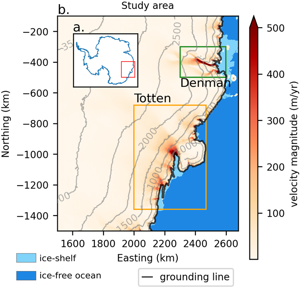
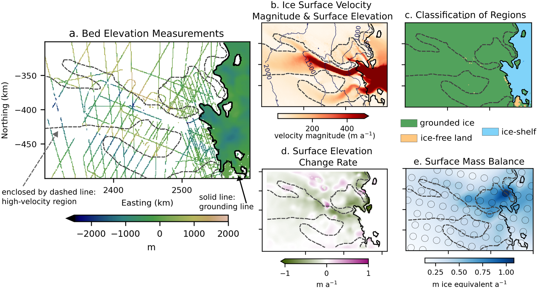

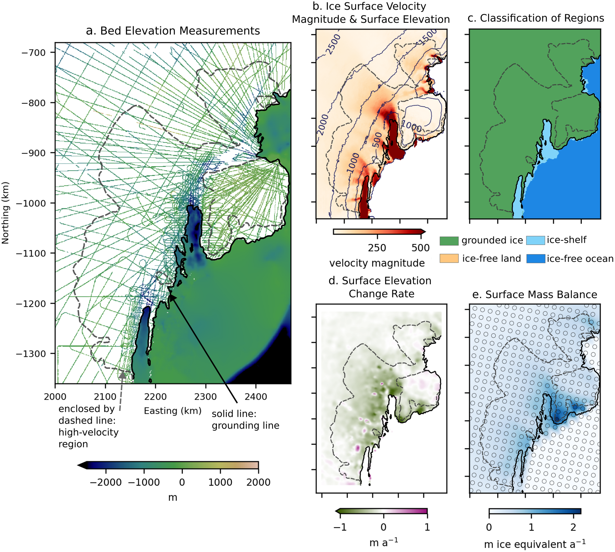

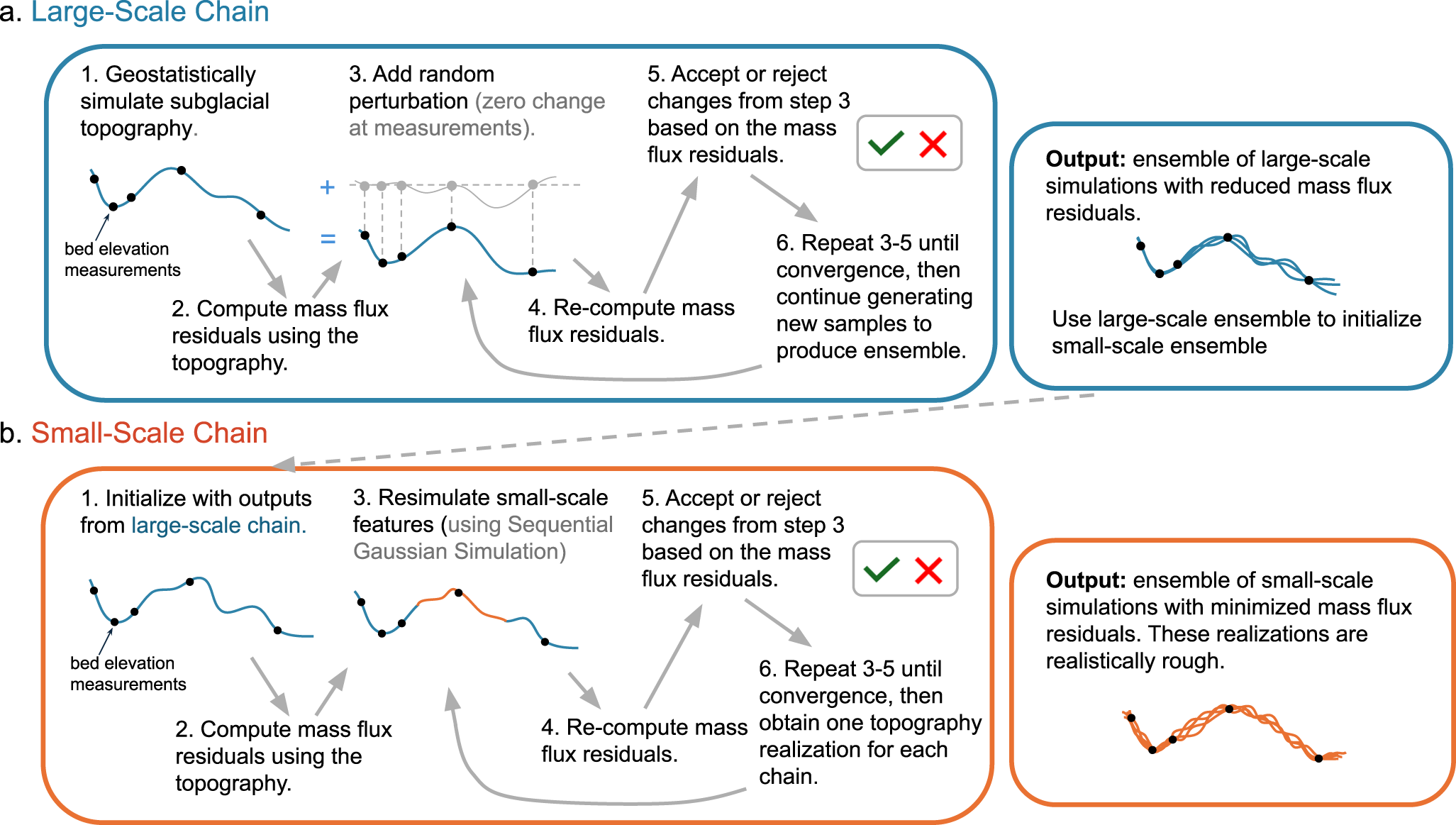
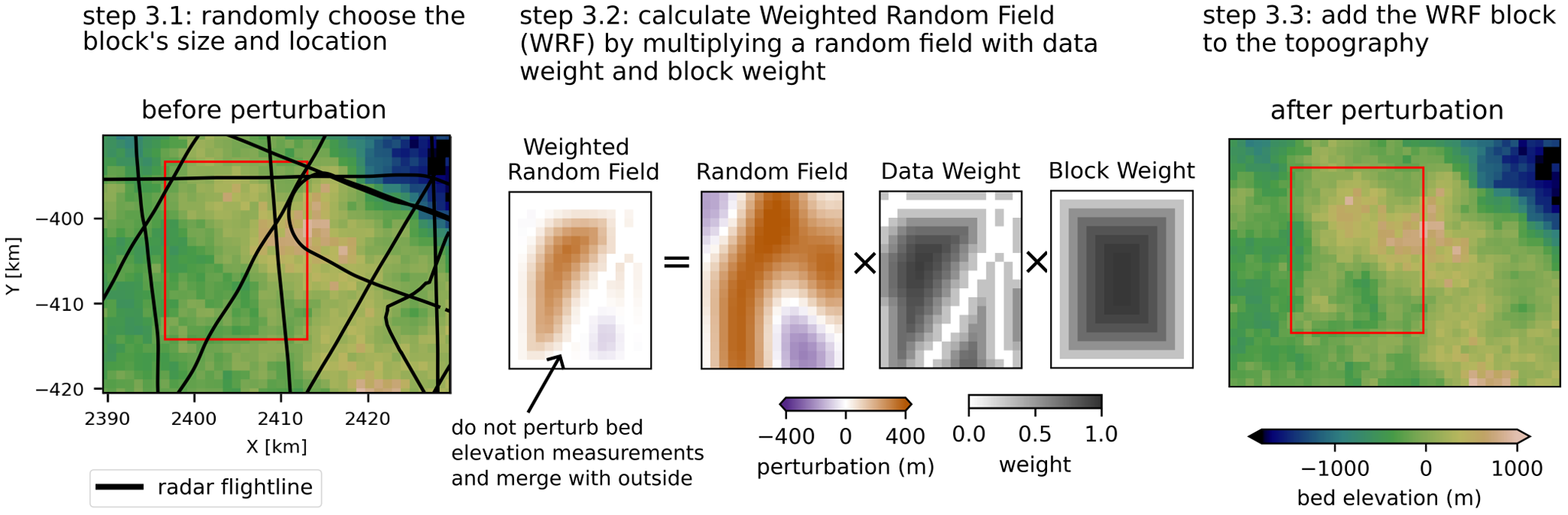
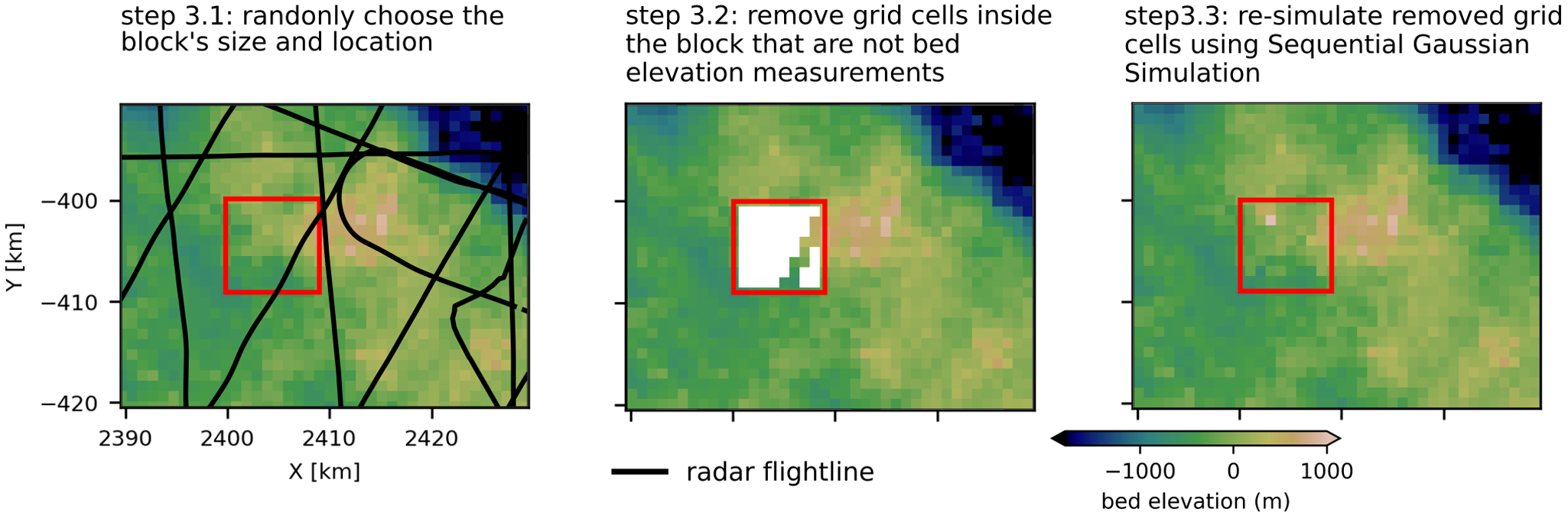
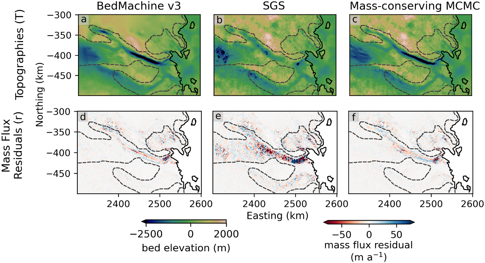
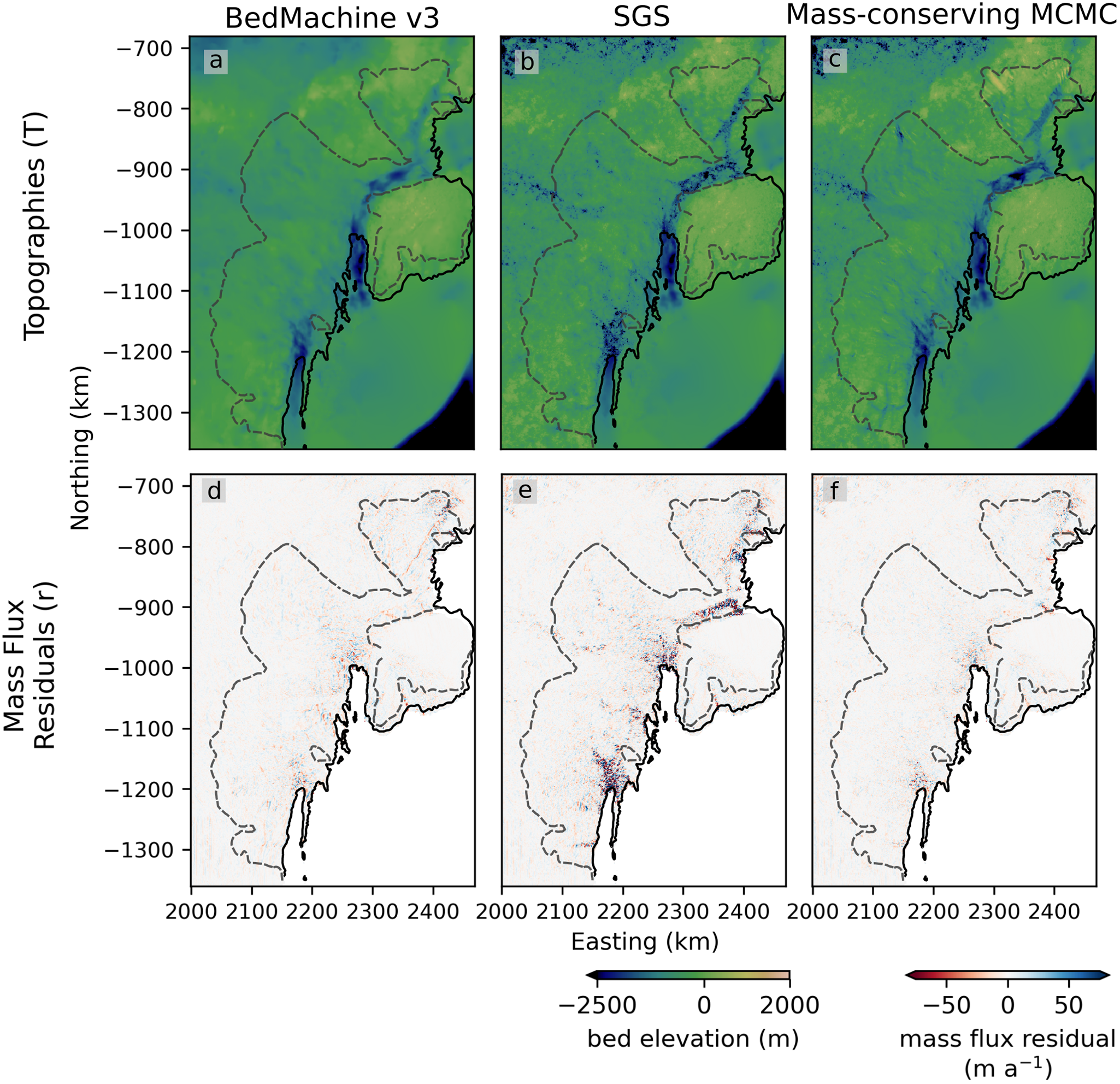
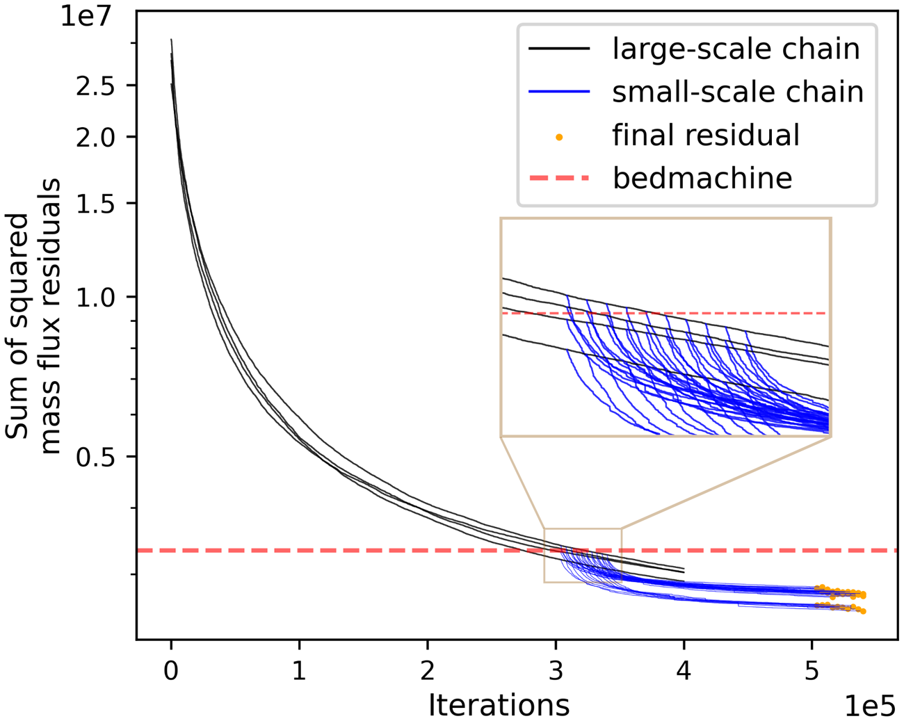
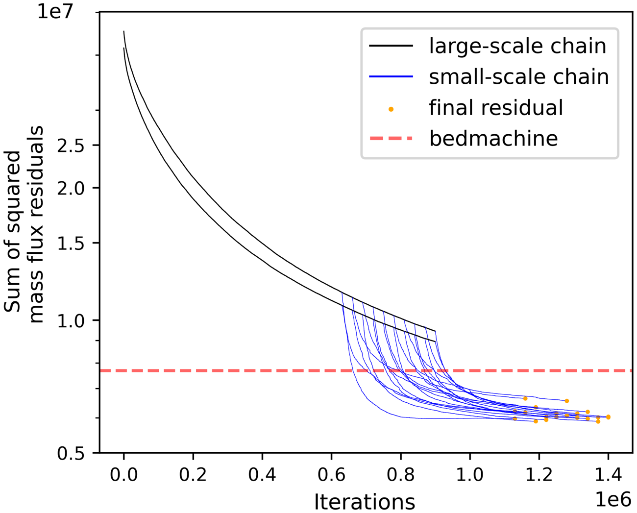
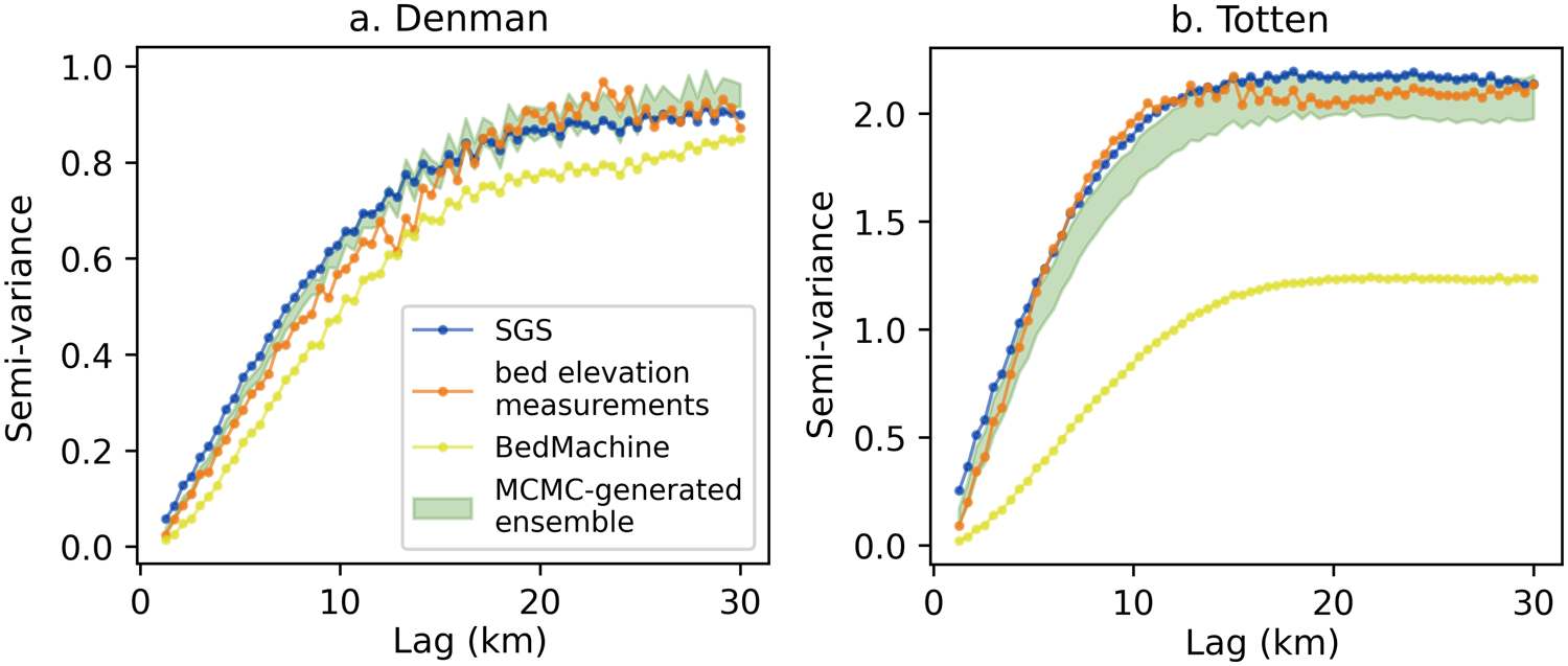
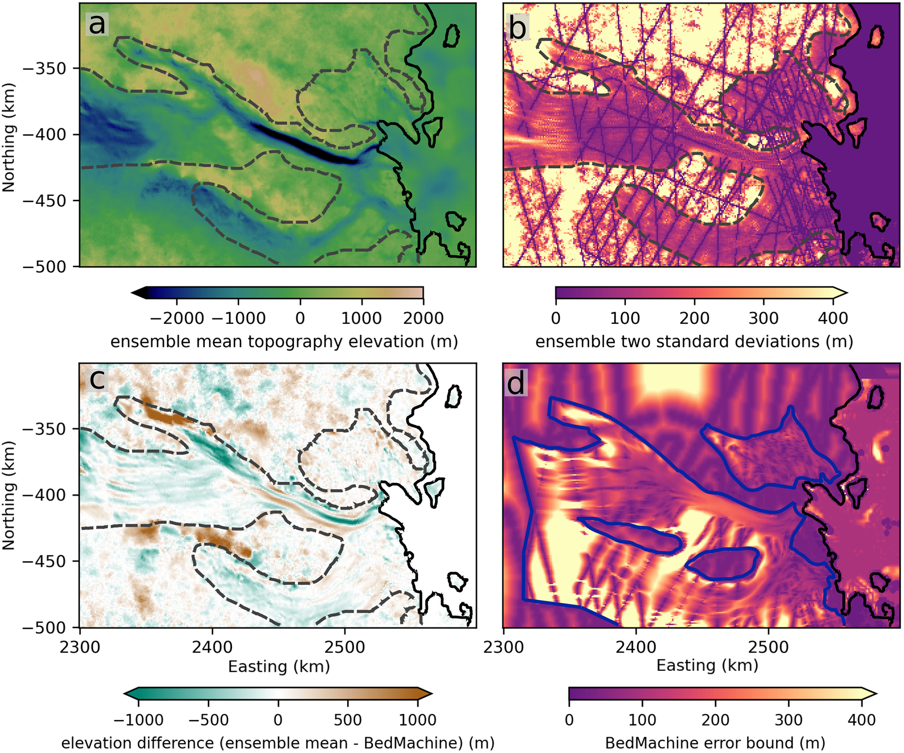
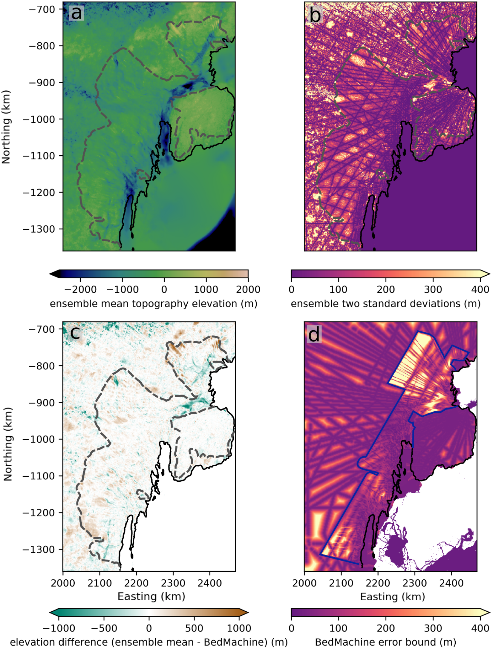
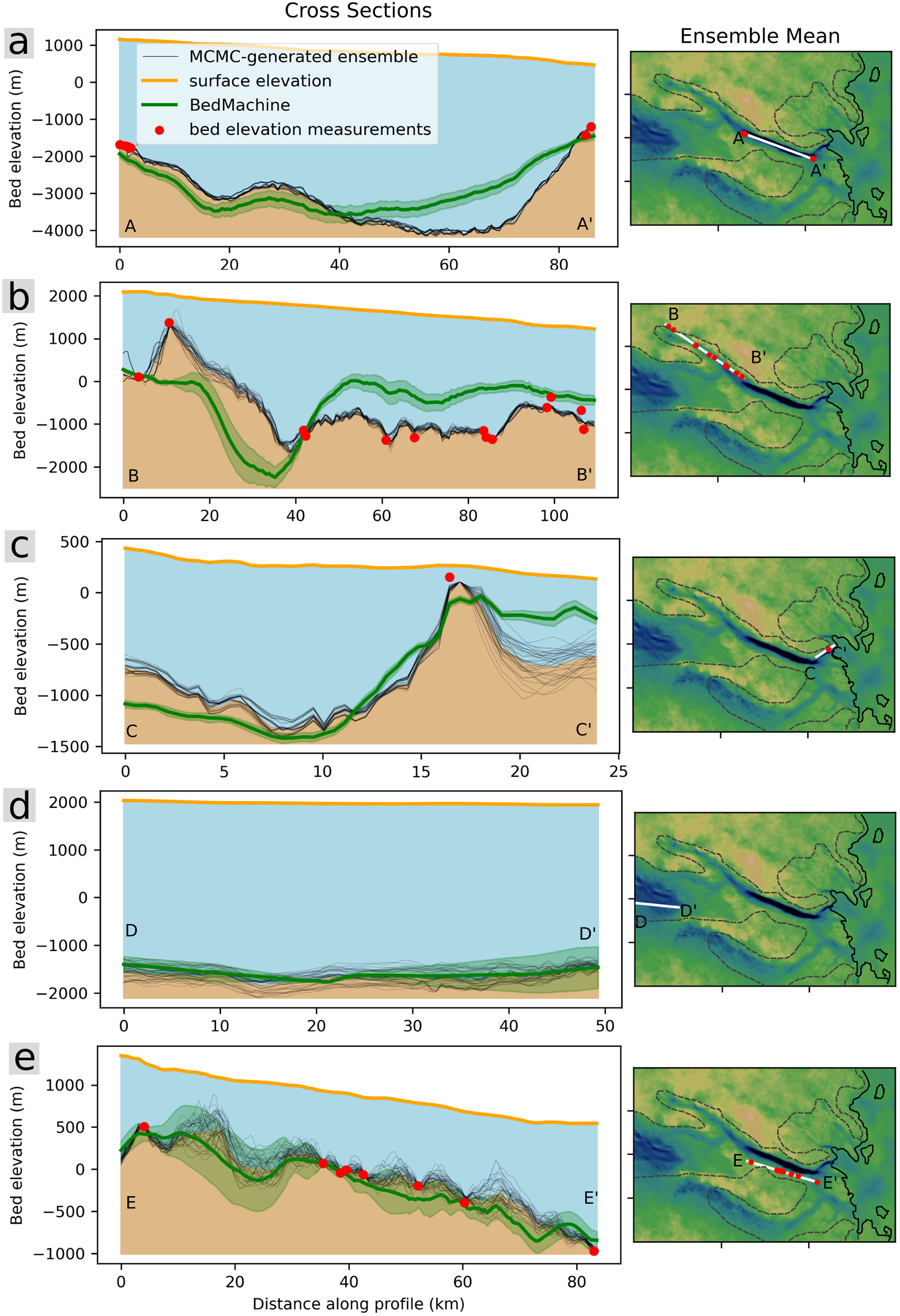
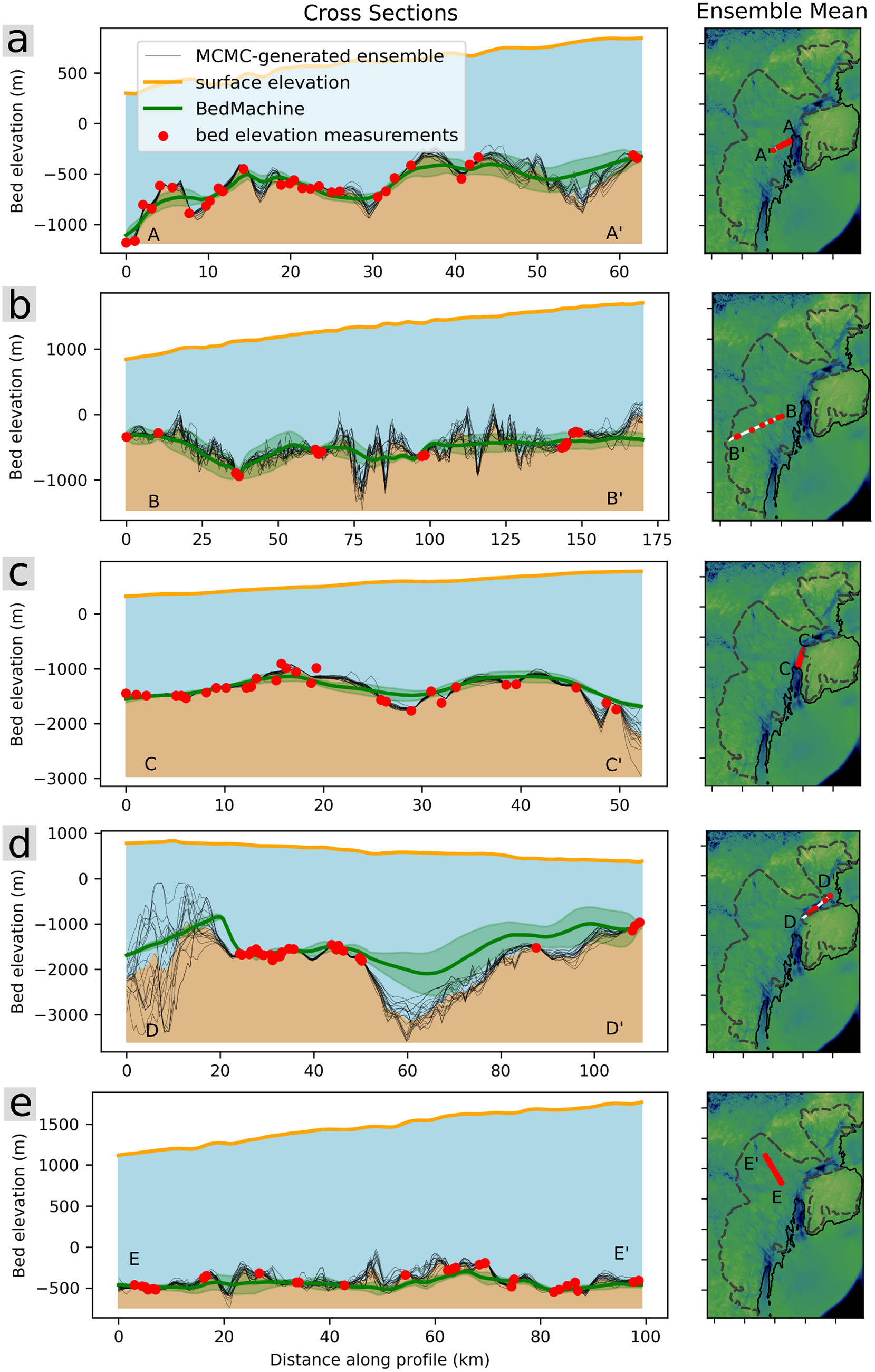


 Open access

