





Impact Statement
Extracting meaningful features from raw data is essential for developing reliable prognostic algorithms, especially when dealing with degenerative phenomena. These cases often involve label-free, multimodal, and noisy data, making preprocessing complex and limiting generalizability. This manuscript introduces a deep monotonic feature extraction model that automatically derives interpretable, deterioration related features from raw data. By focusing on monotonic trends, the model supports robust, domain-adaptable predictions in critical areas such as health care and engineering, where early warnings can significantly impact safety and resource planning.
1. Introduction
In today’s interconnected world, the significance of comprehending and addressing degenerative phenomena across diverse domains remains crucial to the advancement of humanity as a whole. In every facet of our lives, from health care to transportation, from energy production to manufacturing, systems deteriorate over time. The ability to anticipate and proactively address this deterioration has far-reaching implications for enhancing safety, optimizing resource allocation, and improving the overall quality of life (Hobbs, Reference Hobbs2001). In particular, for healthcare and engineering applications, understanding and mitigating deterioration becomes even more crucial. The recognition and understanding of deterioration in medical applications, defined as clinical deterioration, hold paramount importance as it enables timely intervention and proactive management, ultimately safeguarding patient well-being and improving healthcare outcomes (Churpek et al., Reference Churpek, Yuen and Edelson2013; Malycha et al., Reference Malycha, Bacchi and Redfern2022). Simultaneously, the significance of detecting and addressing deterioration in engineering applications cannot be overstated, as it facilitates proactive maintenance and optimization of operations, leading to enhanced productivity, cost-efficiency, and reliability (Wang, Reference Wang2002; Frangopol et al., Reference Frangopol, Sabatino and Soliman2015).
Advancements in technology, such as the Internet of Things and data analytics, have further facilitated the monitoring and management of deteriorating systems. Prognostics—a discipline that strives to anticipate the future behavior of systems based on their current conditions—is the principal component of understanding and predicting future deterioration. By harnessing the power of data-driven insights, prognostic models enable the identification of early warning signs, predict critical events, and facilitate real-time decision making to prevent failures. However, the intrinsic challenges associated with this discipline, including the unsupervised nature of the task, constraints imposed by limited data availability, and the complex nature of understanding deterioration, collectively serve as significant impediments that must be addressed to achieve accurate and predictive outcomes. Thereby, the extraction of features from raw data represents a crucial intermediate step with the potential to facilitate the development of an efficient prognostic framework. Effective feature extraction simplifies the complexity of raw sensor data by reducing noise and identifying the most relevant signals for predicting deterioration. Additionally, it enhances interpretability and reduces computational complexity, thus simplifying the process of constructing prognostic models.
Currently, most prognostic frameworks are designed for specific fields, making them less adaptable to different areas of study. Yet, an increasing demand exists for versatile models capable of functioning across diverse disciplines, driven by the interconnectedness prevalent in modern times. Whether the focus is on healthcare, engineering, or other sectors, systems often overlap. Creating versatile prognostic models that can handle these interdisciplinary challenges is essential. It can provide valuable insights, enhance decision making, and contribute to greater efficiency and resilience in diverse fields. Moreover, there exists an imperative demand for these models to exhibit user-friendliness, enabling individuals who lack expertise in the specific field to employ them without necessitating the creation of individual models on each occasion. This would save both valuable time and resources, making the development of adaptable and accessible models a significant step in addressing complex real-world issues. Clustering techniques have the potential to serve as a solution to this multifaceted problem by enabling the identification of common patterns and behaviors across different domains.
Despite the emerging contribution of machine learning (ML) and deep learning (DL) models concerning predicting degenerative phenomena via feature extraction and clustering techniques to medical and engineering applications, they come up with significant barriers to being easily applicable, adaptable, and transferable to diverse domains. First, it is challenging to extract informative features from noisy raw data (data sparsity) under limited availability (data scarcity) and in an unsupervised manner. On the first hand, the complexity and heterogeneity of medical datasets pose a significant challenge in extracting actionable knowledge from data (Roberts et al., Reference Roberts, Driggs, Thorpe, Gilbey, Yeung, Ursprung and Schönlieb2021; Sapoval et al., Reference Sapoval, Aghazadeh, Nute, Antunes, Balaji, Baraniuk and Treangen2022). On the other hand, engineering systems often consist of datasets with diverse parameters such as vibration patterns, temperature fluctuations, and acoustic emissions. The complexity of those systems, coupled with the vast amounts of data generated by sensors and monitoring devices, presents a significant challenge in extracting relevant information for prognostics.
Second, one of the primary challenges encountered in the clustering process within the context of comprehending the pattern of system deterioration for prognostic applications lies in the extensive preprocessing steps necessary prior to feeding the data into a clustering model (Agarwal et al., Reference Agarwal, Alam and Biswas2011). These preprocessing steps involve the arduous tasks of noise removal, exclusion of irrelevant information, data fusion, and dimensionality reduction, requiring not only considerable time and computational resources, but also domain knowledge (Ezugwu et al., Reference Ezugwu, Ikotun, Oyelade, Abualigah, Agushaka, Eke and Akinyelu2022). This barrier restricts the generalizability of the model to other domains, necessitating a similar exhaustive preprocessing effort and another training process for the new task.
Third, currently, feature extraction models are being developed jointly with the selected prognostic algorithm. Consequently, their efficiency in extracting relevant features is not guaranteed if used with a different prognostic algorithm. In essence, feature extraction is not agnostic to the underlying prognostic algorithm, thus significantly constraining the model’s generalizability.
Finally, current feature extraction models predominantly rely on unimodal inputs (Li et al., Reference Li, Zhang and Ding2019a; Deng et al., Reference Deng, Zhang, Cheng, Zheng, Jiang, Liu and Peng2019; Zhao et al., Reference Zhao, Xu and Chen2021), overlooking the immense potential that multimodal data fusion holds for prognostic-related tasks. Health care and engineering benefit substantially from the integration of diverse data streams encompassing clinical, laboratory, and demographic data (health care) (Salvi et al., Reference Salvi, Loh, Seoni, Barua, García, Molinari and Acharya2024), and a mix of time-series and image sensory data (engineering) (Qiu et al., Reference Qiu, Martínez-Sánchez, Arias-Sánchez and Rashdi2023). However, integrating diverse data modalities often requires addressing issues related to data heterogeneity, varying scales, disparate formats, and inherent noise across different sources. Additionally, it requires specialized expertise, and robust methodologies for alignment and fusion ensuring harmonization among varying data sources (Gravina et al., Reference Gravina, Alinia, Ghasemzadeh and Fortino2017; Zou et al., Reference Zou, Wang, Hu and Han2020; Nazarahari and Rouhani, Reference Nazarahari and Rouhani2021).
The aforementioned challenges are not only detected in healthcare and engineering fields, but they are actively limiting the development of such models to any scientific field related to degenerative phenomena. Hence, creating robust models capable of extracting meaningful patterns and features automatically from any data source is essential for improved performance, generalizability, and robustness. In this regard, the current work introduces a novel unsupervised deep soft monotonic clustering (DSMC) model based on artificial neural networks (ANN) as a fundamental process for feature extraction via clustering analysis in the generic context of deteriorating systems and is showcased on multidisciplinary fields including health care and engineering. The proposed DSMC model is generalizable and agnostic of the chosen prognostic model developed after the clustering process, hence exhibiting promising potential for broader application across various domains beyond those examined in this study. Notably, the novelty of the model lies in its unique capability to extract prognostic-related features, that is, increasing monotonic features as time increases, directly from raw and multimodal data, in an unsupervised and end-to-end manner. The selection of prognostic-related features in the proposed approach aims to capture partial (soft) monotonicity rather than complete (hard) monotonicity. This choice is made to incorporate the potential occurrence of oscillations in the degradation trajectory of the analyzed system. As a result, the DSMC model has the capability to identify certain timestamps within a given trajectory where a substantial recovery may arise, thereby reflecting real-world systems and enabling a certain level of data comprehension.
The proposed model is applied to three carefully selected datasets from distinct scientific domains including health care and engineering, both of significant importance to humanity. The first dataset, known as Medical Information Mart for Intensive Care III (MIMIC-III) (Johnson et al., Reference Johnson, Pollard, Shen, Lehman, Feng, Ghassemi and Mark2016), pertains to the field of health care and encompasses numerous subsets representing diverse life-threatening conditions. For the purpose of this study, the sepsis subset within the MIMIC-III dataset was specifically chosen, given its intricate syndrome nature, substantial healthcare costs, and high mortality rates. In particular, sepsis contributes to 6% of hospitalizations and 35% of in-hospital deaths (Rhee et al., Reference Rhee, Dantes, Epstein, Murphy, Seymour, Iwashyna and Klompas2017) (approximately 30% of patients do not survive longer than 6 months; Buchman et al., Reference Buchman, Simpson, Sciarretta, Finne, Sowers, Collier and Kelman2020) and corresponds to more than $27 billion annually in the United States (Arefian et al., Reference Arefian, Heublein, Scherag, Brunkhorst, Younis and Moerer2017). The diverse multimodal characteristics inherent in this dataset serve as a testament to the challenges encountered by our model in handling and effectively leveraging multiple modes of information. It consists of vital signs, treated as one-dimensional time-series data, and laboratory and demographic data, treated as tabular data.
The second dataset employed in this study is NASA’s Commercial Modular Aero-Propulsion System Simulation (C-MAPSS) (Saxena and Goebel, Reference Saxena and Goebel2008), which is associated with the engineering domain. The utilization of this dataset facilitates the development of prognostic models, contributing to technological advancements, enhanced safety measures, minimized costs, and reduced environmental impact (Vollert and Theissler, Reference Vollert and Theissler2021). This dataset consists of multivariate time-series data and is a proper candidate for comparing the outcomes with different standard techniques.
While these two datasets are recognized for highlighting not only the presence of multimodality (time-series, static data), but also demonstrating the generalizable and robust nature of our model, an additional validation to ascertain the model’s proficiency in handling multimodal information involves the selection of a third dataset from the engineering domain. This dataset concerns an experimental campaign of a structure under fatigue loading (Eleftheroglou, Reference Eleftheroglou2020) and comprises one-, two-, and three-dimensional data concurrently (time series and sequences of images), thereby surpassing the complexity of the C-MAPSS dataset. For the remainder of this article, the third dataset will be named F-MOC (which stands for Fatigue Monitoring of Composites) (Komninos et al., Reference Komninos, Kontogiannis and Eleftheroglou2024). It is worth mentioning that the F-MOC dataset includes real data from the engineering field, unlike the C-MAPSS dataset, which consists of simulated data.
To sum up, the novelty of this work is performing deep soft monotonic feature extraction via clustering in an end-to-end and unsupervised manner with the introduction of the time feature inside the ANN architecture. As such, the monotonic clustering results make the DSMC model agnostic of the chosen prognostic algorithm, ensuring robustness. Additionally, the objectives of this work contain the following:
-
• Extracting soft monotonic features from raw data that could be directly fed as input to any prognostic model.
-
• The soft monotonic feature extraction method should adeptly handle multimodal data.
-
• Application in multidisciplinary domains including degenerative phenomena in a fully automatic fashion. Extensive preprocessing of the data should be avoided, thus a similar architecture can be reproduced, enabling generalizability.
-
• Interpretability of the proposed model to effectively understand its learning process and predicting capabilities.
Each of these datasets achieves one or more of our desired objectives. Particularly, the soft monotonic feature extraction outcomes and the model’s generalizability and interpretability are showcased by all of the datasets. The model’s prognostic algorithm agnosticism is established via the C-MAPSS dataset by demonstrating consistent prognostic outcomes across three distinct ML prognostic models. The evaluation of the proposed model’s performance across multidisciplinary domains is illustrated by utilizing the MIMIC-III dataset. This evaluation involves a comparative analysis of survivability probabilities using various healthcare scoring systems. The handling of multimodal data for soft monotonic feature extraction is majorly validated by the F-MOC dataset. Regarding interpretability, in detail, the flow of the time gradients is illustrated to validate the acceptance of the proposed technique concerning soft monotonicity. Simultaneously, the extracted hidden features are depicted before and after training the DSMC model to justify their role in both capturing the time constraint and performing appropriate clustering.
In summary, the model’s increased versatility and usability highlight its potential for broader application and utility, rendering it capable of effectively tackling substantial challenges that prevent the advancement of humanity and technology.
2. Related work
2.1. Feature extraction for prognostic-related tasks in health care and engineering
In the field of health care, prognostics play a pivotal role in enhancing patient care, optimizing treatment strategies, and allocating healthcare resources effectively (Ling and Huang, Reference Ling and Huang2020; Jiang et al., Reference Jiang, Zhang, Wang, Huang, Chen, Xi and Li2023). In-hospital clinical deterioration may relate to existing or emerging diseases, or a complication of the health care provided. Undoubtedly, by utilizing data-driven techniques, mainly through ML and its subfield, DL, prognostic models can identify new possible biomarkers (Åkesson et al., Reference Åkesson, Hojjati, Hellberg, Raffetseder, Khademi, Rynkowski and Gustafsson2023), detect anomalies (Lee et al., Reference Lee, Jeong, Kim, Jang, Paik, Kang and Kim2022; Shin et al., Reference Shin, Choi, Shim, Kim, Park, Cho and Choi2023), predict disease progression (Ali et al., Reference Ali, El-Sappagh, Islam, Kwak, Ali, Imran and Kwak2020; Chao et al., Reference Chao, Shan, Homayounieh, Singh, Khera, Guo and Yan2021; Li et al., Reference Li, Chen, Li, Wang, Zhao, Lin and Lin2023; Mei et al., Reference Mei, Liu, Singh, Lange, Boddu, Gong and Yang2023; Weiss et al., Reference Weiss, Raghu, Bontempi, Christiani, Mak, Lu and Aerts2023; Zhao et al., Reference Zhao, Chen, Xie, Liu, Hou, Xu and He2023; Zhong et al., Reference Zhong, Cai, Chen, Gui, Deng and Yang2023), and enable personalized treatment plans (Verharen et al., Reference Verharen, de Jong, Roelofs, Huffels, van Zessen, Luijendijk and Vanderschuren2018; Habib et al., Reference Habib, Makhoul, Darazi and Couturier2019; Nakamura et al., Reference Nakamura, Kojima, Uchino, Ono, Yanagita and Murashita2021). Additionally, prognostics also hold immense value in the domain of engineering systems (Jones et al., Reference Jones, Stimming and Lee2022; Peng et al., Reference Peng, Chen, Gui, Tang and Li2022; Kerin et al., Reference Kerin, Hartono and Pham2023; Lu et al., Reference Lu, Xiong, Tian, Wang and Sun2023) as they play a vital role in enhancing system performance and optimizing maintenance strategies.
Prognostic algorithms have great potential, but they face significant challenges, such as working with unlabeled data, limited data availability, and understanding deterioration complexities. Overcoming these obstacles is crucial for accurate predictions. Extracting features from raw data is a key step that could help improve prognostic algorithms in terms of accuracy and robustness. Having this step simplifies the available data, makes it easier to understand, and reduces complexity, making the development of predictive models more versatile.
A comprehensive literature review on state-of-the-art feature extraction techniques for prognostics using deep learning in health care and engineering reveals significant advancements and diverse methodologies. In health care, deep learning models such as convolutional neural networks (CNN) (Ismail et al., Reference Ismail, Hassan, Alsalamah and Fortino2020; Zhao et al., Reference Zhao, Liu, Jin, Dang and Deng2021) and recurrent neural networks (RNN) (Choi et al., Reference Choi, Bahadori, Schuetz, Stewart and Sun2016; Rajkomar et al., Reference Rajkomar, Oren, Chen, Dai, Hajaj, Hardt and Dean2018) have been extensively utilized to extract complex features from medical images and time-series data, respectively, aiding in the prediction of disease progression and patient outcomes. Similarly, in engineering, deep learning techniques are employed to analyze sensor data and identify critical patterns indicative of system health and impending failures. Hybrid models combining CNNs with long short-term memory (LSTM) networks have shown remarkable performance and have been currently the state-of-the-art approaches in capturing both spatial and temporal dependencies, enhancing prognostic accuracy (Zhao et al., Reference Zhao, Yan, Wang and Mao2017; Lei et al., Reference Lei, Li, Guo, Li, Yan and Lin2018). Autoencoders, known for their capability to learn efficient representations of data, can be combined with these approaches to further refine feature extraction by reducing dimensionality and denoising input data, thereby improving the robustness and accuracy of prognostic models (Junbo et al., Reference Junbo, Weining, Juneng and Xueqian2015; Lu et al., Reference Lu, Wang, Yang and Zhang2015; Jia et al., Reference Jia, Lei, Lin, Zhou and Lu2016). Additionally, attention mechanisms are increasingly being integrated to refine feature extraction and improve model generalization across different datasets (Li et al., Reference Li, Zhang and Ding2019b; Chen et al., Reference Chen, Peng, Zhu and Li2020). These advancements underscore the critical role of deep learning in transforming prognostics by providing robust, data-driven insights in both healthcare and engineering domains.
Clustering techniques can offer valuable insights and improve feature extraction in prognostics by grouping similar data points, thereby uncovering inherent structures within the data. This unsupervised learning approach enables the identification of patterns and anomalies that might not be evident through traditional methods. Clustering models have significant potential as feature extractors, serving as a crucial preliminary step preceding the prognostic phase. Model-agnostic feature extraction methods that utilize data-driven clustering can categorize and extract relevant information allowing the development of adaptable and accessible prognostic tools that transcend disciplinary boundaries (Jain et al., Reference Jain, Murty and Flynn1999).
In the context of prognostics, clustering serves as a powerful tool for reducing dimensionality, enhancing interpretability, and improving the accuracy of prognostic models (Warren Liao, Reference Warren Liao2005). Considering health care, this process can unravel patient subgroups with distinct disease trajectories (Al-Fahdawi et al., Reference Al-Fahdawi, Al-Waisy, Zeebaree, Qahwaji, Natiq, Mohammed and Deveci2024), thus enabling tailored interventions and personalized healthcare delivery. For instance, predicting the mortality rate of patients afflicted with sepsis, a life-threatening condition arising from the body’s response to infection, can be achieved through the utilization of clustering and prognostic methodologies (Jang et al., Reference Jang, Yoo, Lee, Uh and Kim2022). By identifying clusters within the patients’ population, it becomes possible to uncover distinct patterns and subgroups that may have different mortality risks. The unique trends and characteristics observed by the clustering analysis can facilitate the development of prognostic models that are able to predict mortality rates with more accurate risk stratification.
Similarly, in the field of engineering systems, clustering techniques can reveal inherent patterns and relationships within sensor data (Gutierrez-Osuna, Reference Gutierrez-Osuna2002), enabling the identification of distinct operational regimes (Wang et al., Reference Wang, Wang, Jiang, Li and Wang2019; Xu et al., Reference Xu, Bashir, Zhang, Yang, Wang and Li2022), detection of anomalies (Li et al., Reference Li, Izakian, Pedrycz and Jamal2021; López et al., Reference López, Aguilera-Martos, García-Barzana, Herrera, García-Gil and Luengo2023), and optimization of maintenance strategies (Santos et al., Reference Santos, Munoz, Olivares, Filho, Ser and de Albuquerque2020; Bousdekis et al., Reference Bousdekis, Lepenioti, Apostolou and Mentzas2021). By integrating clustering techniques into the prognostics workflow, researchers or human experts can leverage the underlying pattern within engineering data, extract representative features, and develop accurate prognostic models easily transferable to varying engineering applications (Diez-Olivan et al., Reference Diez-Olivan, Del Ser, Galar and Sierra2019).
2.2. Multimodal deep clustering
Numerous clustering techniques have been proposed in the literature in the past decades. Deep clustering, an extension of the typical clustering algorithms for tasks with increased data complexity utilizing ANN, has shown promising results in fusing multisensory data and learning useful and interpretable representations. For instance, Xu et al. (Reference Xu, Ren, Shi, Shen and Zhu2023) proposed a unified framework based on ANN with disentangled representation learning that learns interpretable representations by performing multiview clustering, thus achieving multiview information fusion without requiring label supervision. This was accomplished by constructing multiple autoencoders (AEs) for handling each unique kind of information. Then, the embeddings were fused in the disentangled representation phase to keep the meaningful information for clustering. Another work aimed at deep multimodal image fusion and clustering with an application in neuroimaging (Dimitri et al., Reference Dimitri, Spasov, Duggento, Passamonti, Lió and Toschi2022). The key novelty was the combination of deep AE for creating embeddings that were combined with other demographic data extracted from typical ML techniques to cluster the examined patients into subgroups based on the severity of brain damage. Finally, an algorithm that simultaneously learns feature representations and cluster assignments based on ANN was suggested by Xie et al. (Reference Xie, Girshick and Farhadi2015) and evaluated on two image-related and one text-related public datasets.
This study incorporates multimodal data by combining either time-series and static data or a combination of time-series, static data, and sequential images. The novel and distinctive structure of the model confronts the unique challenges posed by multimodality, integrating soft monotonicity within its architecture.
2.3. Monotonic neural networks
The literature on integrating monotonicity within the layers of an ANN has a longstanding history. However, this field came up with significant barriers due to the significant constraints imposed on the parameter space. This resulted in the optimization process being prone to converging toward local optima (Mariotti et al., Reference Mariotti, Alonso Moral and Gatt2023). Nevertheless, the fundamental research in Sill (Reference Sill1998) demonstrated that the universal approximation capabilities of an ANN remain valid under the condition of constraining weights to be positive by leveraging an unconstrained continuous function. Subsequently, building upon this proposition, researchers in Zhang and Zhang (Reference Zhang and Zhang1999) illustrated that the backpropagation algorithm retains its functionality when unconstrained weights are transformed into their exponential counterparts, and all activation functions are assumed to be positive across their entire domain. Activation functions such as the Rectified Linear Unit (ReLU), Sigmoid, or Softmax have been identified as suitable candidates for this purpose. Consequently, weights can assume any real value while their exponential transformation ensures their confinement within the positive domain. Subsequently, numerous studies have adopted similar methodologies to enforce monotonicity within their ANN architectures without constraining the exploration space of parameters (Wehenkel and Louppe, Reference Wehenkel and Louppe2019; Liu et al., Reference Liu, Han, Zhang and Liu2020; Runje and Shankaranarayana, Reference Runje and Shankaranarayana2022).
3. Methodology
In this section, we present the methodology of the current study in detail. Our approach builds on the integration of two prior works: the study by Xie et al. (Reference Xie, Girshick and Farhadi2015)), which performs unsupervised clustering directly from raw data using an ANN, and the study by Zhang and Zhang (Reference Zhang and Zhang1999), which incorporates monotonicity constraints within an ANN architecture. The combination of these two ideas forms the foundation of our proposed ANN design, which we further extend for time-series data and enhance with mechanisms that automatically determine the network architecture, thereby improving robustness.
Figure 1 shows the general concept of this work, beginning from the correct shaping of the data where the time feature is inserted and the technique of sliding windows is applied to the time-series signals. Next, the model construction takes place where the AE extracts the monotonic features to the output of the Z-space used to perform clustering analysis. The training of this model is performed iteratively by utilizing the Bayesian optimization (BO) algorithm (Victoria and Maragatham, Reference Victoria and Maragatham2021) with a customizable objective function for the tuning of the hyperparameters. Finally, the prognostic algorithms are applied to estimate the reliability and survivability curves.
The concept of the proposed methodology.

3.1. Datasets and data shaping
The purpose of this study is to present a generalized monotonic clustering model that can be applied in multidisciplinary domains, can identify deterioration in systems, and prepare monotonic features ready to be fed to any prognostic model in an unsupervised manner with limited training data (5–90 trajectories depending on the dataset). In this regard, two publicly available datasets are examined from entirely different scientific fields. Additionally, a third dataset representing an experimental case study has been chosen for this work. Those datasets were carefully chosen due to their unique characteristics, difficulties, and contributions to health care and engineering.
The MIMIC-III database is a publicly available and widely used database that incorporates patient information from patients hospitalized and stayed in an Intensive Care Unit (ICU) at Beth Israel Deaconess Medical Center (Bowers, Massachusetts, USA) between 2001 and 2012. It contains data about patients’ demographics, vital signs, lab tests, and treatment assignments. From these data, we focused on adult patients fulfilling the international consensus Sepsis-3 criteria (Singer et al., Reference Singer, Deutschman, Seymour, Shankar-Hari, Annane, Bauer and Angus2016) who passed away from sepsis and stayed at the ICU for more than 10 h. Hence, patients who stayed 9 h or less were excluded, as proposed in a previous work (R. Liu et al., Reference Liu, Hunold, Caterino and Zhang2023), due to potentially unreliable measurements. Thus, we extracted data from 62 patients that included nonmissing values for demographics, vital signs, and lab tests. This is the total number of patients who met up with a death event, showcasing a challenging dataset in terms of data scarcity. Vital signs contain the time-series data and demographics, and lab tests contain the supplementary data with the abovementioned time feature included. The unique challenge of this dataset is that it includes both time-series and static input data that should be combined effectively to cluster the severity of the sepsis in terms of mortality rate in an unsupervised manner with a soft monotonic behavior.
Table 1 summarizes the list of patients’ statistics (mean, standard deviation, maximum, minimum, and mode). Two features related to demographics can be identified: the patient’s gender and age. Additionally, similarly to a previous study (R. Liu et al., Reference Liu, Hunold, Caterino and Zhang2023), 15 lab test features are included. From these samples, we kept 52 for training and 10 for testing. To cover patients in the test set from the entire range of staying hours in the ICU, the data were sorted based on these staying hours, and one sample in every six was excluded from the training set. Each sample contains seven input time-series features representing the vital signs and is divided into windows with $ {L}_{window}=10 $
h and step size
$ {L}_{window}=10 $
h and step size $ S=1 $
h, thus creating overlapping windows with
$ S=1 $
h, thus creating overlapping windows with $ 90\% $
overlap. Those samples were normalized feature-wisely to the range [0,1] with min–max normalization according to the training samples. Then, the same statistical values were applied to the testing ones to avoid data leakage. It is noteworthy that any other required preprocessing step does not exist.
$ 90\% $
overlap. Those samples were normalized feature-wisely to the range [0,1] with min–max normalization according to the training samples. Then, the same statistical values were applied to the testing ones to avoid data leakage. It is noteworthy that any other required preprocessing step does not exist.
List of variables extracted by the MIMIC-III dataset

Note. Vital signs represent the time-series inputs. Demographics and lab tests represent the supplementary data.
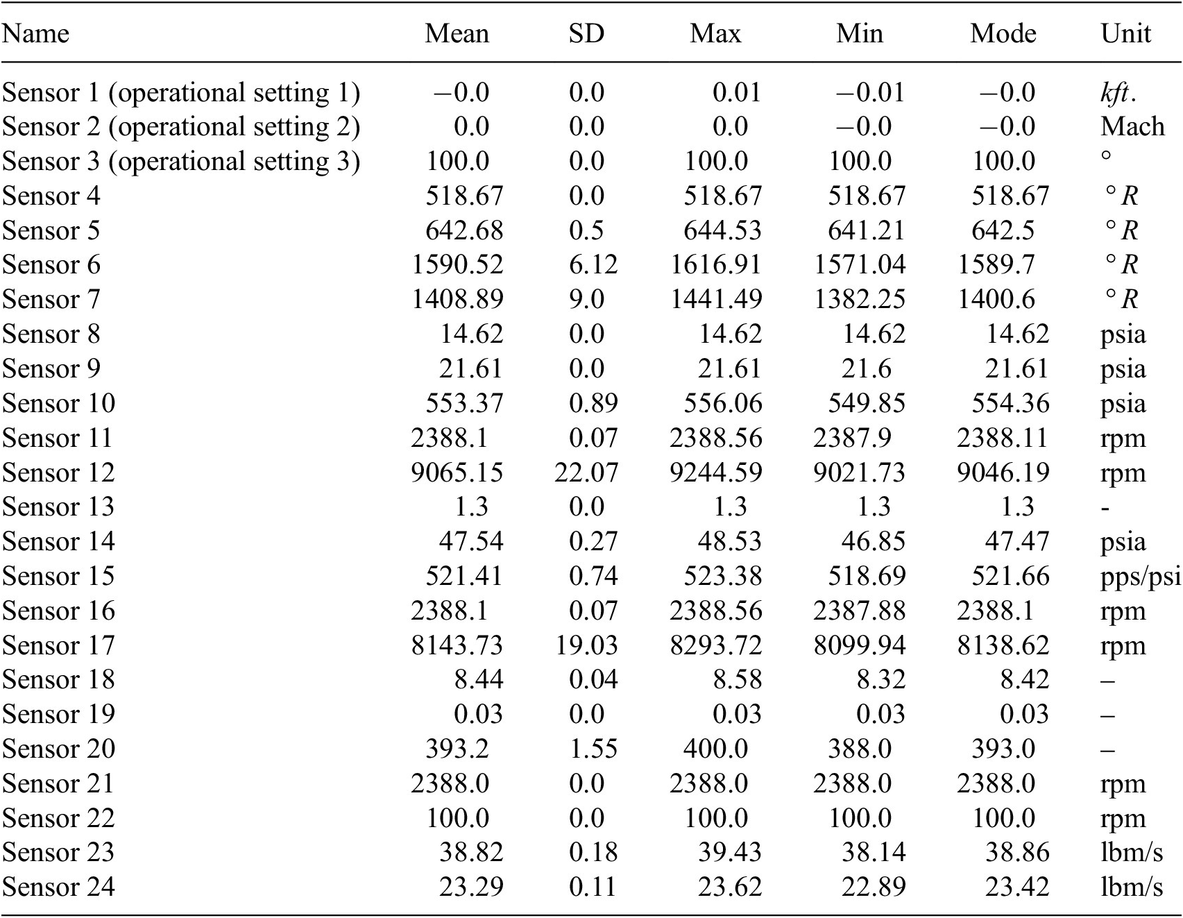
The second examined dataset is NASA’s C-MAPSS dataset which concerns propulsion systems (engines) and represents engineering applications with multivariate time-series sensor data. The C-MAPSS tool is responsible for generating this dataset. This tool models various engine fleet deterioration occurrences from an initial condition (baseline) to the point of failure, concerning the training data and a time period prior to the end of life (EOL) in the test data. Each time series comes from a different engine thus the data can be considered from a fleet of engines of the same type. There are three operational settings (altitude, Mach number, and throttle resolver angle) that have a substantial effect on engine performance. These settings are also included in the data. The data are contaminated with sensor noise. Each engine operates normally at the start of each time series and develops a fault at some point during the series. In the training set, the fault grows in magnitude until system failure. In the test set, the time series ends prior to system failure. Since our focus is on systems that reach the EOL, we consider only the training set as our dataset to be split into train/test samples.
The subset named FD001 is used without excluding any of the sensor signals. The first two columns contain each engine’s ID and deterioration time steps, the next three columns include the three engine’s operational conditions, and the rest 21 columns carry the sensor signals. We kept only the raw sensory information, thus excluding the first 2 columns. The remaining signals can give an increasing, decreasing, or constant trend during the engine’s deterioration which makes it tricky for the model to effectively cluster the severity of the damage in an unsupervised manner. Table 2 summarizes the mean, standard deviation, maximum, minimum, and mode of each sensor.
List of variables extracted by the C-MAPSS dataset
In subset FD001, there are 100 samples where the fault grows in magnitude until system failure. These samples are split into 90 training and 10 test trajectories. To test varying trajectory lengths, the data were sorted and 1 sample in every 10 was excluded from the training set and kept in the testing set. Each sample contains 21 input time-series representing the sensors and they are divided into overlapping windows with $ {L}_{window}=10 $
cycles and step size
$ {L}_{window}=10 $
cycles and step size $ S=1 $
cycle (
$ S=1 $
cycle ( $ 90\% $
overlap). Similarly to MIMIC-III dataset, the data were normalized using min–max normalization according to the training samples to the range
$ 90\% $
overlap). Similarly to MIMIC-III dataset, the data were normalized using min–max normalization according to the training samples to the range $ \left[0,1\right] $
, feature-wisely, and the same statistical values were applied to the testing samples. In this dataset, there are no other supplementary data besides the time feature.
$ \left[0,1\right] $
, feature-wisely, and the same statistical values were applied to the testing samples. In this dataset, there are no other supplementary data besides the time feature.
The third dataset is the F-MOC dataset, that is, an experimental campaign developed in Eleftheroglou (Reference Eleftheroglou2020). This experiment investigates the fatigue behavior of a unidirectional prepreg tape Hexply® F6376CHTS(12K)-5-35 laminate. The laminate is first manufactured and then cured in an autoclave as per manufacturer recommendations and specimens of standardized dimensions are obtained. Fatigue loading is applied using a Mechanical Testing System (MTS) controller on a bench fatigue machine. Images during pause intervals were captured using specialized cameras. The loading protocol involves cyclic loading with specified intervals and load transitions to analyze the laminate’s fatigue behavior under varying stress conditions. The sensor system consists of two cameras for Digital Image Correlation (DIC) measurements and an acoustic emission system with a sampling rate of 2 MHz. The measurements were taken until the specimen’s failure point. The acoustic emission low-level features were extracted by an AMSY-6 Vallen Systeme GmbH. From these features, the ones summarized in Table 3 were considered. The threshold value is defined at $ 50 $ $ dB $
, that is, the acoustic emission signals that have an amplitude less than
$ dB $
, that is, the acoustic emission signals that have an amplitude less than $ 50 $ $ dB $
(
$ dB $
( $ \approx 3.16 $ $ \mu V $
) were discarded.
$ \mu V $
) were discarded.
The low-level features that are considered and extracted by the AMSY-6 Vallen Systeme GmbH

In this dataset, there are seven trajectories of acoustic emission and DIC data representing seven specimens, respectively. The lifetime, the number of images used, and the size of the acoustic emission and DIC data of each specimen are summarized in Table 4. To overcome memory issues, we kept only the data from the first camera and discarded the rest. Furthermore, we scaled down the image dimensions from a resolution of $ \left[2048\times 1024\right] $
to
$ \left[2048\times 1024\right] $
to $ \left[128\times 64\right] $
via an average pooling filter. The synchronization process of the images and acoustic emission data is described in Appendix B.2. According to this process, it was chosen
$ \left[128\times 64\right] $
via an average pooling filter. The synchronization process of the images and acoustic emission data is described in Appendix B.2. According to this process, it was chosen $ {L}_{window}=6 $
images with
$ {L}_{window}=6 $
images with $ S=3 $
images. The corresponding variables for the acoustic emission are calculated based on the synchronization. Similarly to the previous datasets, the only preprocessing step is normalization to the range
$ S=3 $
images. The corresponding variables for the acoustic emission are calculated based on the synchronization. Similarly to the previous datasets, the only preprocessing step is normalization to the range $ \left[0,1\right] $
. For the gray-scale image, this normalization is simply a division with the value 255 which corresponds to a pixel with a white color. For the acoustic emission signals, each sample was normalized feature-wisely, similarly to the two aforementioned datasets.
$ \left[0,1\right] $
. For the gray-scale image, this normalization is simply a division with the value 255 which corresponds to a pixel with a white color. For the acoustic emission signals, each sample was normalized feature-wisely, similarly to the two aforementioned datasets.
General characteristics of the F-MOC dataset

There are three types of data examined in this study: time series, static data, and time frames. Each trajectory is split into short overlapping windows of length $ {L}_{window} $
and step size
$ {L}_{window} $
and step size $ S $
. Since the F-MOC dataset requires synchronization of the inputs as there is a conflict between active (DIC) and passive (acoustic emission) testing methods, the value of
$ S $
. Since the F-MOC dataset requires synchronization of the inputs as there is a conflict between active (DIC) and passive (acoustic emission) testing methods, the value of $ {L}_{window} $
is determined based on the sampling rate of the DIC process, which is 50 sec. More details about synchronization can be found in Appendix B.2. Following the synchronization process, a configuration was established where six sequential images were integrated into a time frame, and concurrently, each acoustic emission signal was standardized to a length of
$ {L}_{window} $
is determined based on the sampling rate of the DIC process, which is 50 sec. More details about synchronization can be found in Appendix B.2. Following the synchronization process, a configuration was established where six sequential images were integrated into a time frame, and concurrently, each acoustic emission signal was standardized to a length of $ 300 $
s. This pairing of a time frame and its corresponding acoustic signal signifies a single window. The determination of subsequent windows involved an overlapping scheme, with the fourth image of the preceding window aligning with the first image of the succeeding window (thus,
$ 300 $
s. This pairing of a time frame and its corresponding acoustic signal signifies a single window. The determination of subsequent windows involved an overlapping scheme, with the fourth image of the preceding window aligning with the first image of the succeeding window (thus, $ S=3 $
). Consequently, the initial window comprised images 1–6, while the subsequent window included images 4–9, and so forth. Based on the synchronization process, a similar overlap is applied to the acoustic emission signals. The same procedure of overlapping windows is followed for the C-MAPSS and MIMIC-III datasets, without the synchronization step as only one-dimensional signals exist. It is noteworthy that the hyperparameters
$ S=3 $
). Consequently, the initial window comprised images 1–6, while the subsequent window included images 4–9, and so forth. Based on the synchronization process, a similar overlap is applied to the acoustic emission signals. The same procedure of overlapping windows is followed for the C-MAPSS and MIMIC-III datasets, without the synchronization step as only one-dimensional signals exist. It is noteworthy that the hyperparameters $ {L}_{window} $
and
$ {L}_{window} $
and $ S $
of the C-MAPSS and MIMIC-III datasets are not required to match those within the F-MOC dataset.
$ S $
of the C-MAPSS and MIMIC-III datasets are not required to match those within the F-MOC dataset.
For each dataset, the percentage of overlapping can be calculated by the formula $ \left({L}_{window}-S\right)/\left({L}_{window}\right)100\% $
. Depending on the position of the window into the trajectory, a value is assigned to the time feature. These values can be defined in any range with the only constraint of increasing monotonically with the constructed windows of the corresponding trajectory. A straightforward approach to defining the range of time feature values is to simply count the current number of windows that have been constructed and assign that value to
$ \left({L}_{window}-S\right)/\left({L}_{window}\right)100\% $
. Depending on the position of the window into the trajectory, a value is assigned to the time feature. These values can be defined in any range with the only constraint of increasing monotonically with the constructed windows of the corresponding trajectory. A straightforward approach to defining the range of time feature values is to simply count the current number of windows that have been constructed and assign that value to $ t $
starting from
$ t $
starting from $ t=0 $
for the first window of the trajectory,
$ t=0 $
for the first window of the trajectory, $ t=1 $
for the second, and so on. Unfortunately, this setup may give an unbalanced learning process if the trajectory lengths vary seriously. To mitigate this pitfall, an alternative approach is to calculate the average trajectory length
$ t=1 $
for the second, and so on. Unfortunately, this setup may give an unbalanced learning process if the trajectory lengths vary seriously. To mitigate this pitfall, an alternative approach is to calculate the average trajectory length $ {L}_{avg} $
given all the lengths of the training trajectories, and then apply a linear spacing for
$ {L}_{avg} $
given all the lengths of the training trajectories, and then apply a linear spacing for $ t $
depending on each trajectory length. In this regard, for each trajectory, the time feature is bounded in the range of
$ t $
depending on each trajectory length. In this regard, for each trajectory, the time feature is bounded in the range of $ \left[0,{L}_{avg}\right] $
. The intermediate values are then linearly spaced between those extremes according to the current trajectory length. In detail, for each trajectory of length
$ \left[0,{L}_{avg}\right] $
. The intermediate values are then linearly spaced between those extremes according to the current trajectory length. In detail, for each trajectory of length $ L $
, the time feature array is constructed to be
$ L $
, the time feature array is constructed to be $ t=\left[0,\frac{L_{avg}}{L},\frac{2{L}_{avg}}{L},\dots, {L}_{avg}\right] $
.
$ t=\left[0,\frac{L_{avg}}{L},\frac{2{L}_{avg}}{L},\dots, {L}_{avg}\right] $
.
In summary, each sample should contain a window consisting of time series data and the corresponding scalar value of the time feature which constitutes one feature of the static data. Additional static data are considered for the MIMIC-III dataset, that is, demographic and lab test data, defined as supplementary data. The F-MOC dataset consists of overlapping windows of synchronized time series and frames (three-dimensional data).
3.2. Model architecture
The concept of employing end-to-end feature extraction and then clustering utilizing a raw input data space $ X $
requires a transformation of those inputs into an
$ X $
requires a transformation of those inputs into an $ D $
-dimensional embedding space
$ D $
-dimensional embedding space $ {Z}^D $
, where
$ {Z}^D $
, where $ D $
is typically much lower than the dimension of
$ D $
is typically much lower than the dimension of $ X $
, with a nonlinear mapping
$ X $
, with a nonlinear mapping $ {f}_{\theta }(X)=Z $
, where
$ {f}_{\theta }(X)=Z $
, where $ f $
is a function approximator and
$ f $
is a function approximator and $ \theta $
its parameters. The extraction of valuable information from raw data entails the utilization of a complex function that involves intricate mathematical operations. ANN naturally emerges as a suitable choice for this purpose due to their theoretical function approximation properties and their demonstrated feature learning capabilities (Hornik, Reference Hornik1991). In the context of deteriorating systems, the input data typically comprises trajectories, predominantly in the form of time series. The first layer of the ANN should be responsible for extracting time-related information, thereby making the LSTM (Hochreiter and Schmidhuber, Reference Hochreiter and Schmidhuber1997), that is, a recurrent layer an appropriate candidate. Subsequently, the remaining layers can consist of stacked fully connected (FC) layers. Notably, supplementary data, that is, nonsequential data that give additional unique information for each sample, can be introduced into one of these FC layers, enabling their integration into the DSMC model and tackling the unique challenges of multimodal data.
$ \theta $
its parameters. The extraction of valuable information from raw data entails the utilization of a complex function that involves intricate mathematical operations. ANN naturally emerges as a suitable choice for this purpose due to their theoretical function approximation properties and their demonstrated feature learning capabilities (Hornik, Reference Hornik1991). In the context of deteriorating systems, the input data typically comprises trajectories, predominantly in the form of time series. The first layer of the ANN should be responsible for extracting time-related information, thereby making the LSTM (Hochreiter and Schmidhuber, Reference Hochreiter and Schmidhuber1997), that is, a recurrent layer an appropriate candidate. Subsequently, the remaining layers can consist of stacked fully connected (FC) layers. Notably, supplementary data, that is, nonsequential data that give additional unique information for each sample, can be introduced into one of these FC layers, enabling their integration into the DSMC model and tackling the unique challenges of multimodal data.
The DSMC model is ultimately a modified encoder that simultaneously extracts prognostic-related features and clusters those features accordingly. Training the DSMC model requires a two-stage training process: a pretraining of the encoder via a deep AE, and a following training process of the encoder that enables its output, namely, the Z-space, to assign cluster labels to the incoming input data. In the first stage, the AE setup is shown at a high level in Figure 2a. It consists of two modules stacked with multiple layers each. The first module, the feature extractor module, hiddenly extracts information from the input data via a set of LSTM layers, as shown in Figure 2b. It is possible to cover any kind of sequential data (time series, frames, etc.) by adapting the first layer(s) of the feature extractor module according to the examined domain. For instance, if the input contains one-dimensional time series data, then a typical LSTM layer is enough to capture the temporal hidden features of the sequence. If the input contains image sequences, such as sequential CT scans (Brugnara et al., Reference Brugnara, Baumgartner, Scholze, Deike-Hofmann, Kades, Scherer and Vollmuth2023) or time-resolved segmentations (Müller et al., Reference Müller, Sauter, Shunmugasundaram, Wenzler, De Andrade and De Carlo2021), then a Convolutional LSTM or a three-dimensional CNN (CNN3D) could be used. Importantly, a mix of one-, two-, and three-dimensional sequential data could be provided at once by combining the abovementioned types of layers inside the feature extractor module. This efficiently enables the applicability of the proposed model to any kind of sequential input data.
(a) Module-level architecture of the proposed AE model. (b) Detailed architecture of the proposed AE model. (c) Detailed architecture of the DSMC model used for soft monotonic clustering.

The second module, referred to as the monotonic module, comprises a stacked configuration of FC layers with an incorporated monotonic modification, serving as a pivotal factor in extracting monotonic-related features. To establish this monotonicity, it is important to apply a hard constraint between the time feature $ t $
and the output
$ t $
and the output $ z $
. For each sample
$ z $
. For each sample $ i $
, we want the gradients of
$ i $
, we want the gradients of $ {z}_i $
with respect to
$ {z}_i $
with respect to $ {t}_i $
to be non-negative, that is,
$ {t}_i $
to be non-negative, that is,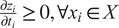 $ \frac{\partial {z}_i}{\partial {t}_i}\ge 0,\forall {x}_i\in X $
. For an MLP, it is proven in Zhang and Zhang (Reference Zhang and Zhang1999) that the output is increasing (decreasing) monotonically with respect to input, if and only if the weights and the activation functions of input, output, and intermediate layers are always increasing (decreasing). The corresponding biases can have any real value since they do not affect the outputs’ gradients. In this regard, by employing an exponential operation on the weights of each neuron in every layer, ranging from the input layer to the output layer of the monotonic module (see Figure 2a), we ensure the desired monotonicity. This approach to enforcing monotonous constraints allows the weights to assume any real value during the learning process, without imposing any limitations on the weight space. Since these constraints are applied inside the structure of the network during the forward pass, the typical backpropagation algorithm can be used by satisfying the converging properties of the ANN. Consider the typical formulation of a neuron to be:
$ \frac{\partial {z}_i}{\partial {t}_i}\ge 0,\forall {x}_i\in X $
. For an MLP, it is proven in Zhang and Zhang (Reference Zhang and Zhang1999) that the output is increasing (decreasing) monotonically with respect to input, if and only if the weights and the activation functions of input, output, and intermediate layers are always increasing (decreasing). The corresponding biases can have any real value since they do not affect the outputs’ gradients. In this regard, by employing an exponential operation on the weights of each neuron in every layer, ranging from the input layer to the output layer of the monotonic module (see Figure 2a), we ensure the desired monotonicity. This approach to enforcing monotonous constraints allows the weights to assume any real value during the learning process, without imposing any limitations on the weight space. Since these constraints are applied inside the structure of the network during the forward pass, the typical backpropagation algorithm can be used by satisfying the converging properties of the ANN. Consider the typical formulation of a neuron to be:
 $$ {r}_v={b}_v+\sum \limits_u{w}_{uv}g\left({r}_u\right), $$
where $ b $
is the bias,
$ b $
is the bias, $ w $
the weights that come from neuron
$ w $
the weights that come from neuron $ u $
of the previous layer and contribute to the current layer’s neuron
$ u $
of the previous layer and contribute to the current layer’s neuron $ v $
, and
$ v $
, and $ g(.) $
the activation function, hence
$ g(.) $
the activation function, hence $ g\left({r}_u\right) $
is the output of the neuron
$ g\left({r}_u\right) $
is the output of the neuron $ u $
that comes from the previous layer (i.e., the input of the current layer
$ u $
that comes from the previous layer (i.e., the input of the current layer $ v $
). By applying the desired non-negative monotonic constraints to the neurons we have:
$ v $
). By applying the desired non-negative monotonic constraints to the neurons we have:
 $$ {r}_v={b}_v+\sum \limits_u{e}^{w_{uv}}g\left({r}_u\right),g\ge 0,{g}^{\prime}\ge 0\hskip0.6em everywhere. $$
The gradients with respect to the bias remain the same, while the gradients concerning the weights used for backpropagation are transformed by the partial derivative of $ {r}_v $
with respect to
$ {r}_v $
with respect to $ {w}_{uv} $
as:
$ {w}_{uv} $
as:
 $$ \frac{\partial {r}_v}{\partial {w}_{uv}}=g\left({r}_u\right)\hskip0.1em {e}^{w_{uv}}. $$
By the chain rule, the gradient of the loss with respect to $ {w}_{uv} $
becomes:
$ {w}_{uv} $
becomes:
 $$ \frac{\partial \mathrm{Loss}}{\partial {w}_{uv}}=\frac{\partial {r}_v}{\partial {w}_{uv}}\cdot \frac{\partial \mathrm{Loss}}{\partial {r}_v}. $$
Substituting the expression for $ \frac{\partial {r}_v}{\partial {w}_{uv}} $
gives:
$ \frac{\partial {r}_v}{\partial {w}_{uv}} $
gives:
 $$ \frac{\partial Loss}{\partial {w}_{uv}}=g\left({r}_u\right){e}^{w_{uv}}\frac{\partial \mathrm{Loss}}{\partial {r}_v}. $$
There are two crucial advantages of using this approach for achieving monotonicity. First, monotonicity can be optionally applied in a sub-group of FC layers. Consequently, the rest of the ANN architecture which may contain other kinds of layers than FC could remain unchanged. Second, it is possible to have soft monotonicity between inputs and outputs, simply by applying an exponential operation only to the weights concerning the input which is under the examined constraint. For input variables such constraints are not required, thus the weights may remain unchanged to allow more flexibility. Both of the aforementioned attributes are desirable for our architecture since we need monotonic constraints only with respect to the time feature which, simultaneously, should be inserted into an intermediate layer. As a result, monotonic relationships are exclusively attained within the monotonic module, specifically within the neurons influenced by the time feature for generating the output. This clarifies why, despite the existence of a hard monotonic constraint between $ Z $
and
$ Z $
and $ t $
, a soft monotonic behavior between
$ t $
, a soft monotonic behavior between $ Z $
and
$ Z $
and $ X $
is observed, ultimately leading to the desired soft monotonic clustering.
$ X $
is observed, ultimately leading to the desired soft monotonic clustering.
Except for the main contributing layers of the DSMC model shown in Figure 2b and c, between each layer, dropout and parametric batch-normalization (BN) layers are involved. An important observation is that the gradient outputs of BN layers can have a heavy impact on the monotonic constraints during backpropagation. To address this issue, we applied the same exponential function to the weights of each BN layer as applied similarly to the rest of the layers of the monotonic module described in Equation 2, without affecting the corresponding biases. After the final LSTM layer of the feature extractor, a flattening layer without any trainable parameters was applied to transform the array into one-dimensional before inputting it to the FC layers. The activation function used after the LSTM layers corresponded to Tanh, while a Softplus function was used after every FC layer to ensure a positive monotonic increase. It should be noted that the FC layers that are applied before the monotonic module can be followed by any kind of activation function. The same layers are applied to the decoder.
Together, these two modules form both the encoder and decoder components. The decoder progressively increases the dimensionality through its layer-by-layer construction and is responsible for simultaneously reconstructing the input sequential data, the supplementary data, and the time feature. Once the data exits the monotonic module, the time feature is no longer required and is subsequently removed from the decoder. Given the vital role played by the supplementary data in the learning process, we allow the AE to utilize this information implicitly, without any modifications.
Having the encoder pretrained via the AE setup, the deep clustering part which is based on Xie et al. (Reference Xie, Girshick and Farhadi2015) is taking place. In this approach, deep clustering seeks to cluster the input data points into $ K $
clusters by simultaneously learning the parameters
$ K $
clusters by simultaneously learning the parameters $ \theta $
of the ANN and the cluster centers
$ \theta $
of the ANN and the cluster centers $ {\left\{{\mu}_{\mathrm{j}}\in Z\right\}}_{j=1}^K $
. In this regard, each output
$ {\left\{{\mu}_{\mathrm{j}}\in Z\right\}}_{j=1}^K $
. In this regard, each output $ z\in {Z}^D $
of the encoder is fed to a k-means clustering algorithm for initializing the centroids
$ z\in {Z}^D $
of the encoder is fed to a k-means clustering algorithm for initializing the centroids $ {\mu}_j^d,d\in \left[0,1,\dots, D\right] $
. The process of centroid initialization is applied only once for the entire training dataset. Subsequently, the encoder undergoes additional training with the objective of bringing the encoder output
$ {\mu}_j^d,d\in \left[0,1,\dots, D\right] $
. The process of centroid initialization is applied only once for the entire training dataset. Subsequently, the encoder undergoes additional training with the objective of bringing the encoder output $ z $
and the corresponding centroid
$ z $
and the corresponding centroid $ \mu $
closer to each other. This is achieved through the computation of a soft assignment probability distribution
$ \mu $
closer to each other. This is achieved through the computation of a soft assignment probability distribution $ q $
that establishes the relationship between them and by the utilization of an auxiliary target distribution
$ q $
that establishes the relationship between them and by the utilization of an auxiliary target distribution $ p $
. By minimizing the Kullback–Leibler (KL) divergence between
$ p $
. By minimizing the Kullback–Leibler (KL) divergence between $ q $
and
$ q $
and $ p $
, the goal is to make these distributions similar to each other. The probability distribution
$ p $
, the goal is to make these distributions similar to each other. The probability distribution $ q $
corresponds to the Student’s t distribution which measures the similarity between
$ q $
corresponds to the Student’s t distribution which measures the similarity between $ z $
and
$ z $
and $ \mu $
as follows:
$ \mu $
as follows:
 $$ {q}_{ij}=\frac{{\left(1+{\left\Vert {z}_i-{\mu}_j\right\Vert}^2/\nu \right)}^{-\frac{\nu +1}{2}}}{\sum_{j^{'}}{\left(1+{\left\Vert {z}_i-{\mu}_{j^{'}}\right\Vert}^2/\nu \right)}^{-\frac{\nu +1}{2}}}, $$
where $ \nu $
is the degrees of freedom of the Student’s t distribution and in an unsupervised setting should be fixed to
$ \nu $
is the degrees of freedom of the Student’s t distribution and in an unsupervised setting should be fixed to $ \nu =1 $
. Similarly to Xie et al. (Reference Xie, Girshick and Farhadi2015), the target distribution is chosen to be:
$ \nu =1 $
. Similarly to Xie et al. (Reference Xie, Girshick and Farhadi2015), the target distribution is chosen to be:
 $$ {p}_{ij}=\frac{q_{ij}^2/{\sum}_i{q}_{ij}}{\sum_{j^{\prime }}{q}_{i{j}^{\prime}}^2/{\sum}_i{q}_{i{j}^{\prime }}}. $$
Then the loss function (KL-loss) for training the deep clustering is:
 $$ {Loss}^{DSMC}=\sum \limits_i\sum \limits_j\ {p}_{ij}\log \frac{p_{ij}}{q_{ij}}. $$
The primary concept behind this setup is to adopt a self-learning framework for the model, allowing it to autonomously learn the assignments to clusters with both high and low confidence. The model then focuses on enhancing the assignments that exhibit low confidence. The optimization proceeds by jointly optimizing the ANN’s parameters $ \theta $
and the cluster centroids
$ \theta $
and the cluster centroids $ {\mu}_j $
using the stochastic gradient descent algorithm with momentum and applying a standard backpropagation with respect to
$ {\mu}_j $
using the stochastic gradient descent algorithm with momentum and applying a standard backpropagation with respect to $ \theta $
. The gradients are computed as:
$ \theta $
. The gradients are computed as:
 $$ \frac{\partial {Loss}^{DSMC}}{\partial {z}_i}=\frac{\nu +1}{\nu}\sum \limits_j{\left(1+\frac{{\left\Vert {z}_i-{\mu}_j\right\Vert}^2}{\nu}\right)}^{-1}\times \left({p}_{ij}-{q}_{ij}\right)\left({z}_i-{\mu}_j\right), $$
 $$ \frac{\partial {Loss}^{DSMC}}{\partial {\mu}_j}=-\frac{\nu +1}{\nu}\sum \limits_i{\left(1+\frac{{\left\Vert {z}_i-{\mu}_j\right\Vert}^2}{\nu}\right)}^{-1}\times \left({p}_{ij}-{q}_{ij}\right)\left({z}_i-{\mu}_j\right). $$
During the evaluation of the model, each sample $ {x}_i $
from the input data space
$ {x}_i $
from the input data space $ X $
is transformed by the model into the embedding space
$ X $
is transformed by the model into the embedding space $ {z}_d^i $
which in turn is assigned to a cluster as follows:
$ {z}_d^i $
which in turn is assigned to a cluster as follows:
 $$ {\mathrm{cluster}}^i=\underset{d\in D}{\max}\left(\underset{\hskip0.84em j}{\arg \min}\left({\left\{{\mu}_{jd}^i\right\}}_{j=1}^K-{z}_d^i\right)\right), $$
where
 $$ {z}_d^i={f}_{\theta}\left({x}_s\right),d\in \left[0,1,\dots, D\right]. $$
In the expression before, the inner operation is $ D $
-dimensional representing
$ D $
-dimensional representing $ D $
cluster assignments for the same sample
$ D $
cluster assignments for the same sample $ i $
. This should be reduced to one cluster assignment. To prioritize safety, we have opted to select the maximum assignment (outer operation) as the final prediction. As a result, although there may be an overestimation of the deterioration, the approach significantly mitigates the risk of reaching the end of life (adopting a risk-averse policy; Kahneman and Tversky, Reference Kahneman and Tversky1984; Cao et al., Reference Cao, Wang, Bai, Zhao, Li, Lv and Liu2023).
$ i $
. This should be reduced to one cluster assignment. To prioritize safety, we have opted to select the maximum assignment (outer operation) as the final prediction. As a result, although there may be an overestimation of the deterioration, the approach significantly mitigates the risk of reaching the end of life (adopting a risk-averse policy; Kahneman and Tversky, Reference Kahneman and Tversky1984; Cao et al., Reference Cao, Wang, Bai, Zhao, Li, Lv and Liu2023).
3.2.1. Adaptation of the model’s architecture for the F-MOC dataset
The general architecture of the model remains the same, with the only alternation being in the feature extractor module of the AE. Since there are both time-series (acoustic emission) and three-dimensional (sequences of images) data, the LSTM layers do not suffice to produce the inputs $ {H}_{in}^{enc} $
which are fed to the monotonic module. Consequently, a stack of CNN3D layers is added parallel to the LSTM layers from which hidden features
$ {H}_{in}^{enc} $
which are fed to the monotonic module. Consequently, a stack of CNN3D layers is added parallel to the LSTM layers from which hidden features $ {H}_{in, image}^{enc} $
related to the sequential images are extracted and fused with the hidden features
$ {H}_{in, image}^{enc} $
related to the sequential images are extracted and fused with the hidden features $ {H}_{in, acoustic}^{enc} $
related to the acoustic emission signals. An alternative to the CNN3D layers could be a Convolutional LSTM layer (Chao et al., Reference Chao, Pu, Yin, Han and Chen2018), that is, a combination of CNN and LSTM layers. However, due to the layer’s increased computational power that emerged from its recurrent nature, the CNN3D layer remains the best option. Then, those features are concatenated and passed through an FC layer to produce the required dimensionality of
$ {H}_{in, acoustic}^{enc} $
related to the acoustic emission signals. An alternative to the CNN3D layers could be a Convolutional LSTM layer (Chao et al., Reference Chao, Pu, Yin, Han and Chen2018), that is, a combination of CNN and LSTM layers. However, due to the layer’s increased computational power that emerged from its recurrent nature, the CNN3D layer remains the best option. Then, those features are concatenated and passed through an FC layer to produce the required dimensionality of $ {H}_{in}^{enc} $
.
$ {H}_{in}^{enc} $
.
This process is depicted in Figure 3. The feature extractor of the decoder performs the reverse process of the encoder, thus having the same number of layers and dimensions. This time the input of the encoder and the reconstructed input (output of decoder), $ X $
and
$ X $
and $ {X}^{\prime } $
, respectively, is a set of sequential images representing a time frame and a window of acoustic emission data. Subsequent to minor adjustments in both the clustering process and the prognostic model, the number of clusters has been expanded from
$ {X}^{\prime } $
, respectively, is a set of sequential images representing a time frame and a window of acoustic emission data. Subsequent to minor adjustments in both the clustering process and the prognostic model, the number of clusters has been expanded from $ 10 $
to
$ 10 $
to $ 30 $
, reflecting the increased trajectory lengths. This modification aims to enhance the model’s capability to capture more extensive information pertaining to the progression of damage in the structure. Table 5 summarizes the hyperparameters related to LSTM and CNN3D. The hyperparameters of LSTM remain unchanged for all datasets except
$ 30 $
, reflecting the increased trajectory lengths. This modification aims to enhance the model’s capability to capture more extensive information pertaining to the progression of damage in the structure. Table 5 summarizes the hyperparameters related to LSTM and CNN3D. The hyperparameters of LSTM remain unchanged for all datasets except $ {H}_{in}^{enc} $
, which is optimized by the BO algorithm per dataset.
$ {H}_{in}^{enc} $
, which is optimized by the BO algorithm per dataset.
Redesigned architecture of the model regarding the F-MOC dataset.

Hyperparameters’ values for the LSTM and CNN3D layers

Note. The LSTM layers remain unchanged for all datasets with the corresponding values of $ {H}_{in}^{enc} $
.
$ {H}_{in}^{enc} $
.
3.3. Training the DSMC model
To train the AE according to the proposed architecture, we modified the typical reconstruction loss (original and reconstructed input) with two additional terms: the reconstruction of time and the reconstruction of the monotonic module. Consider the outcome of the input layer of the encoder’s monotonic module and the outcome of the output layer of the decoder’s monotonic module to be $ {O}_{in}^{enc} $
and
$ {O}_{in}^{enc} $
and $ {O}_{out}^{dec} $
, respectively. Then the loss function used for training the AE is given as follows:
$ {O}_{out}^{dec} $
, respectively. Then the loss function used for training the AE is given as follows:
 $$ {\mathrm{Loss}}^{AE}=\mathrm{MSE}\left(X,{X}^{\prime}\right)+\alpha \cdot \left[\mathrm{MSE}\left(t,{t}^{\prime}\right)+\mathrm{MSE}\left({O}_{\mathrm{in}}^{\mathrm{enc}},{O}_{\mathrm{out}}^{\mathrm{dec}}\right)\right], $$
where $ \mathrm{MSE}(.) $
is the mean squared error,
$ \mathrm{MSE}(.) $
is the mean squared error, $ \alpha $
is a tunable hyperparameter, and
$ \alpha $
is a tunable hyperparameter, and $ {X}^{\prime } $
,
$ {X}^{\prime } $
, $ {t}^{\prime } $
are the reconstructed input and time, respectively. Ultimately, the hyperparameter
$ {t}^{\prime } $
are the reconstructed input and time, respectively. Ultimately, the hyperparameter $ \alpha $
weights the importance that should be given to the monotonic behavior of the clustering. When the AE is trained, we keep only the encoder as a pretrained module, initialize the centroids, and further train it using a combination of
$ \alpha $
weights the importance that should be given to the monotonic behavior of the clustering. When the AE is trained, we keep only the encoder as a pretrained module, initialize the centroids, and further train it using a combination of $ {Loss}^{AE} $
and
$ {Loss}^{AE} $
and $ {Loss}^{DSMC} $
as follows:
$ {Loss}^{DSMC} $
as follows:
 $$ \mathrm{Loss}={\mathrm{Loss}}^{DSMC}+\beta \ast {\mathrm{Loss}}^{AE}, $$
where $ \beta $
is another tunable hyperparameter weighting the contribution of the
$ \beta $
is another tunable hyperparameter weighting the contribution of the $ {Loss}^{AE} $
. The reason for reusing the
$ {Loss}^{AE} $
. The reason for reusing the $ {Loss}^{AE} $
for the clustering process is that we need to keep the soft monotonic nature of the embedding space, which would have gradually vanished otherwise.
$ {Loss}^{AE} $
for the clustering process is that we need to keep the soft monotonic nature of the embedding space, which would have gradually vanished otherwise.
3.4. Bayesian optimization for hyperparameter tuning
Pretraining the encoder via the AE model and then further training it inside the DSMC model in an end-to-end manner poses significant challenges due to the unsupervised learning nature and the presence of multiple loss terms. The effectiveness of these models heavily relies on the setting of their hyperparameters. Manually tuning these hyperparameters can be a time-consuming and labor-intensive task, demanding substantial effort. In this regard, the BO algorithm is chosen as the optimization algorithm for tuning the most important hyperparameters of the two models. BO requires a target function, namely the objective function, to be maximized during the optimization process. This framework is well suited for ANN as it relaxes the constraint of solely relying on continuous loss functions for training purposes. Consequently, the ANN can be trained with its own continuous loss function and its hyperparameters could be tuned with a more efficient, noncontinuous objective function.
Instead of utilizing the proposed $ Loss $
(in its negative form, as the optimization process involves maximization), we have the flexibility to choose any function related to the clustering task that exhibits favorable maximization properties as the objective function for the BO algorithm. In our study, manual hyperparameter tuning revealed two consistent behaviors: (i) substantial transitions from lower clusters to higher ones and (ii) long sequences of values remaining in the ultimate cluster (particularly in larger trajectories). Both observations reflect the trade-off between the time feature and the input time-series data when forming cluster predictions.
$ Loss $
(in its negative form, as the optimization process involves maximization), we have the flexibility to choose any function related to the clustering task that exhibits favorable maximization properties as the objective function for the BO algorithm. In our study, manual hyperparameter tuning revealed two consistent behaviors: (i) substantial transitions from lower clusters to higher ones and (ii) long sequences of values remaining in the ultimate cluster (particularly in larger trajectories). Both observations reflect the trade-off between the time feature and the input time-series data when forming cluster predictions.
To encode these observations into an optimization criterion, the BO algorithm must evaluate hyperparameters using an objective function that (i) rewards smooth progression across clusters, (ii) penalizes excessive jumps between clusters, (iii) penalizes staying indefinitely in the ultimate cluster, and (iv) allows occasional backward transitions to preserve soft monotonicity (i.e., avoiding the trivial solution where the model relies only on the time feature).
Formally, this is expressed as follows. For each trajectory $ j $
, and for each time step
$ j $
, and for each time step $ i $
within the trajectory, let
$ i $
within the trajectory, let
 $$ {\mathrm{d}}_{{\mathrm{c}}_{\mathrm{i}}}={\mathrm{c}}_{\mathrm{i}}-{\mathrm{c}}_{\mathrm{i}-1} $$
denote the difference between the predicted labels at consecutive time steps. Then the objective function optimized by BO is:
 $$ \underset{\mathrm{h}}{\mathrm{argmax}}\left(\frac{\sum_{\mathrm{j}=0}^{{\mathrm{N}}_{\mathrm{traj}}}{\sum}_{\mathrm{i}=1}^{{\mathrm{L}}_{\mathrm{traj}}^{\mathrm{j}}-1}\left[0.6\ast {1}_{{\mathrm{d}}_{{\mathrm{c}}_{\mathrm{i}}}<0}-\left({1}_{\left|{\mathrm{d}}_{{\mathrm{c}}_{\mathrm{i}}}\right|>1}+{1}_{\begin{array}{c}{\mathrm{d}}_{{\mathrm{c}}_{\mathrm{i}}}=0\\ {}{\mathrm{c}}_{\mathrm{i}}=\mathrm{K}-1\end{array}}\right)\right]}{N_{traj}}\right), $$
where $ {N}_{traj} $
is the number of the training trajectories and
$ {N}_{traj} $
is the number of the training trajectories and $ {1}_{condition} $
is equal to one if the condition is satisfied. Here, the reward term
$ {1}_{condition} $
is equal to one if the condition is satisfied. Here, the reward term $ 0.6\cdot {1}_{{\mathrm{d}}_{c_i}<0} $
promotes occasional backward transitions (soft monotonicity). The penalty
$ 0.6\cdot {1}_{{\mathrm{d}}_{c_i}<0} $
promotes occasional backward transitions (soft monotonicity). The penalty $ {1}_{\mid {\mathrm{d}}_{c_i}\mid >1} $
discourages cluster jumps larger than one step. The penalty
$ {1}_{\mid {\mathrm{d}}_{c_i}\mid >1} $
discourages cluster jumps larger than one step. The penalty $ {1}_{{\mathrm{d}}_{c_i}=0,{c}_i=K-1} $
prevents long stationary sequences in the ultimate cluster. The coefficient
$ {1}_{{\mathrm{d}}_{c_i}=0,{c}_i=K-1} $
prevents long stationary sequences in the ultimate cluster. The coefficient $ 0.6 $
was selected empirically to balance the trade-off between promoting backward transitions and preventing degenerate behavior. A lower weight (e.g.,
$ 0.6 $
was selected empirically to balance the trade-off between promoting backward transitions and preventing degenerate behavior. A lower weight (e.g., $ <0.5 $
) made backward transitions too rare, leading to overly strict monotonicity, while a higher weight (e.g., close to
$ <0.5 $
) made backward transitions too rare, leading to overly strict monotonicity, while a higher weight (e.g., close to $ 1 $
) allowed too many reversals, undermining the sequential progression. The value
$ 1 $
) allowed too many reversals, undermining the sequential progression. The value $ 0.6 $
thus represents a compromise: it permits occasional reversals without overwhelming the primary monotonic trend. Optimization is happening on hyperparameters
$ 0.6 $
thus represents a compromise: it permits occasional reversals without overwhelming the primary monotonic trend. Optimization is happening on hyperparameters $ h=\left\{{L}_{window},S,Z,{H}_{in}^{enc},{lr}^{AE},{lr}^{DSMC},{epochs}^{AE},{epochs}^{DSMC},\alpha, \beta, {dr}_{rate}\right\} $
. The hyperparameter
$ h=\left\{{L}_{window},S,Z,{H}_{in}^{enc},{lr}^{AE},{lr}^{DSMC},{epochs}^{AE},{epochs}^{DSMC},\alpha, \beta, {dr}_{rate}\right\} $
. The hyperparameter $ {H}_{in}^{enc} $
corresponds to the number of neurons of the last hidden layer of the encoder’s feature extractor module, and
$ {H}_{in}^{enc} $
corresponds to the number of neurons of the last hidden layer of the encoder’s feature extractor module, and $ {dr}_{rate} $
is the dropout rate.
$ {dr}_{rate} $
is the dropout rate.
Thus, Eq. (16) directly encodes the desired balance; it promotes mostly monotonic progression while still allowing controlled flexibility. All of the hyperparameters $ h $
used in the BO algorithm plus four additional ones that were manually decided, including
$ h $
used in the BO algorithm plus four additional ones that were manually decided, including $ {L}_{window} $
,
$ {L}_{window} $
, $ S $
,
$ S $
, $ {batch}^{AE} $
, and
$ {batch}^{AE} $
, and $ {batch}^{DSMC} $
, are stored in Table 6 for each case study. These values were optimized after 100 iterations. The rationale for selecting these search ranges is grounded in trial-and-error, initially informed by the default values used in previous studies related to the MIMIC-III (Scherpf et al., Reference Scherpf, Gräßer, Malberg and Zaunseder2019; Zebin et al., Reference Zebin, Rezvy and Chaussalet2019) and C-MAPSS (Asif et al., Reference Asif, Haider, Naqvi, Zaki, Kwak and Islam2022; Fu et al., Reference Fu, Zhong, Lin and Zhao2022) datasets. For the F-MOC dataset and the newly introduced hyperparameters in this work, only a trial-and-error approach was followed. Each range was deemed appropriate as long as the BO algorithm identified a hyperparameter that was not positioned near one of the extremes.
$ {batch}^{DSMC} $
, are stored in Table 6 for each case study. These values were optimized after 100 iterations. The rationale for selecting these search ranges is grounded in trial-and-error, initially informed by the default values used in previous studies related to the MIMIC-III (Scherpf et al., Reference Scherpf, Gräßer, Malberg and Zaunseder2019; Zebin et al., Reference Zebin, Rezvy and Chaussalet2019) and C-MAPSS (Asif et al., Reference Asif, Haider, Naqvi, Zaki, Kwak and Islam2022; Fu et al., Reference Fu, Zhong, Lin and Zhao2022) datasets. For the F-MOC dataset and the newly introduced hyperparameters in this work, only a trial-and-error approach was followed. Each range was deemed appropriate as long as the BO algorithm identified a hyperparameter that was not positioned near one of the extremes.
Hyperparameter search ranges and final values optimized by the Bayesian optimization algorithm for each dataset

Note. Both the automatically and manually tuned hyperparameters are included.
3.5. Prognostics
Although this study focuses on monotonic feature extraction and clustering to produce simple expressions that can be easily fed to any prognostic model to make predictions, for comprehensiveness, we utilized the Hidden Semi-Markov Model (HSMM) (Kont et al., Reference Kontogiannis, Salinas-Camus and Eleftheroglou2025) for the prognostic task assuming Gaussian distributions for the observations. Particularly, seven hidden states were chosen and the model was trained for a maximum of 100 iterations or until the convergence tolerance of $ 0.5 $
is met.
$ 0.5 $
is met.
4. Results
In this section, first, the results concerning the MIMIC-III and C-MAPSS datasets are presented and compared. Next, we justify that the model’s behavior is compatible with the aforementioned theory and interpret its behavior. Finally, the results of the F-MOC dataset, which represents a more complicated dataset, are discussed.
The DSMC model was trained on a single GPU (NVIDIA GeForce RTX 2080). The entire training process alongside the hyperparameter tuning via the BO algorithm is approximately 8 h for the MIMIC-III and C-MAPSS datasets, while the computational time is increased substantially for the F-MOC dataset up to approximately 110 h. This arises because BO involves conducting 100 iterations over the hyperparameter space, necessitating the training of the model anew in each iteration. Modifying the number of iterations has the potential to reduce computational effort, but it may concurrently result in a decrease in accuracy.
4.1. Clustering results and survivability analysis of the MIMIC-III and C-MAPSS datasets
Running the DSMC model without BO takes approximately 20 min for each of the first two datasets. The convergence of the training and validating loss corresponding to the reconstruction and time losses, respectively, is shown in the first four subfigures of Figure A3. Running the training process with different weight initialization may produce a variety of loss values. Therefore, we present the reproducibility of our training process via Table A1 which depicts the mean and standard deviation of the training and validating losses. These statistics were produced by running the entire training process 10 times after initializing the ANN’s weights via a Uniform distribution.
After pretraining the encoder at the first stage of the DSMC model’s training, we proceed to the clustering process, the second stage of training. The clustering results for each of the test trajectories are presented in Figure 4 for the two underlying datasets. It should be highlighted that a higher cluster prediction within the context of this study corresponds to a state that is more proximate to the most severe condition. This is due to the introduced monotonicity based on time which is ever-increasing, thus a higher cluster value is associated with a larger timestamp. Specifically, in the case of the MIMIC-III dataset, a higher cluster indicates a state that is closer to a 100% mortality rate. Similarly, for the C-MAPSS dataset, a higher cluster assignment signifies a state that is closer to the structure’s EOL. In the context of both datasets, a deliberate selection of 10 clusters has been made, each associated with labels ranging from 0 to 9. This strategic choice has been made with the primary intention of elucidating the inherent soft monotonicity present within the cluster assignments. The rationale behind opting for precisely 10 clusters lies in the desire to avoid excessive complexity that would render the resulting clustering solution less comprehensible and interpretable. The introduction of a greater number of clusters would inadvertently introduce additional fluctuations that could potentially obscure the underlying patterns, diminishing the clarity of the analysis. Another cluster label equal to 10 is added at the end of each trajectory indicating the last data point of that trajectory. This is to explicitly provide a physical meaning to the last value representing the EOL and, by no means, is used during the testing phase where the last data points are unseen and unknown.
(a) Clustering results for the MIMIC-III dataset. (b) Kaplan–Meier curves for the MIMIC-III dataset (“h” stands for “hours”). (c) Clustering results for the C-MAPSS dataset. (d) Kaplan–Meier curves for the C-MAPSS dataset (“c” stands for “cycles”).

In relation to the MIMIC-III dataset, it is observed in Figure 4a that the labels assigned to the clusters exhibit a monotonic increase, with few exceptions in specific instances where there is an observed improvement in the patient’s health. Given that the model is correctly trained, this decrease in cluster labels can be attributed solely to changes in the corresponding vital signs. From a data-centric perspective, the observed anomaly in the cluster labels can be attributed to irregularities in one or more of the provided input values corresponding to vital signs. Such anomalies may arise from either the presence of noisy data within the dataset or specific treatments administered to the patients. The latter scenario aligns with medical reasoning, as certain treatments can introduce anomalies in the monotonic behavior of the clusters. Consequently, by assuming that the input data is devoid of noise, we posit that a sudden decrease in cluster labels is closely associated with potential self-recovery or temporary improvement in a patient’s condition resulting from a given treatment. However, establishing a direct correlation between the treatment and vital signs measurements is challenging. In preceding research (Moss and Prescott, Reference Moss and Prescott2019), it was observed that the prompt initiation of antibiotic treatment could potentially result in significant adverse effects, including elevated mortality rates. Nevertheless, even if such a correlation could be identified, the accurate determination of the specific time delay required for the effects of the treatment to manifest in the patient under examination remains uncertain.
The prognostic results are presented by the Kaplan–Meier curve (Kaplan and Meier, Reference Kaplan and Meier1958), shown in Figure 4b for the true survivability of the testing population and the corresponding 0, 42, 79, 121, 160, 200, 283, 352, 392, and 812 h predicted survival plots of the same population, respectively. These hours correspond to the time each patient stayed in the ICU until mortality. Hence, these curves indicate the prediction improvement toward the ground truth as more information is available with the elapsed time. Notably, except at 0 h where no information is available and the predictions for all the patients are based only on the mean mortality of the training set, every other survival curve becomes increasingly more informative. Even though the right outlier is not predicted accurately, the prediction provided is mildly conservative and thus not harmful to the model’s overall safety. Since these plots are interconnected based on time, the corresponding p values (log-rank test) are expected to be high, thus being unable to reject the null hypothesis that these plots are similar. This phenomenon is occurring as expected, and for the sake of thoroughness, the p values between the ground truth and each of the other plots are provided, respectively.
In contrast to the majority of related studies (Islam et al., Reference Islam, Nasrin, Walther, Wu, Yang and Li2019; Kong et al., Reference Kong, Lin and Hu2020; Lauritsen et al., Reference Lauritsen, Kristensen, Olsen, Larsen, Lauritsen and Jørgensen2020; Wu et al., Reference Wu, Zhang, Nie, Hong, Zhu, Chen and Li2023) that approach mortality prediction as a classification problem and assess their model’s performance using receiver operating characteristic curves as diagnostic tools, we maintain its inherent nature and consider it as a regression process. Consequently, we show in Figure A1 the survivability rates at 0%, 25%, 50%, and 75% of the corresponding trajectory lengths for four of the test patients, notably for patients 6, 7, 8, and 9. These curves alongside the corresponding reliability curves discussed next concerning the C-MAPSS dataset are derived from the utilization of the HSMM outcomes as described in Kont et al. (Reference Kontogiannis, Salinas-Camus and Eleftheroglou2025).
Regarding the clustering outcomes obtained from the C-MAPSS dataset, Figure 4c reveals the presence of significant fluctuations in the assignments of clusters. These fluctuations are observed in a reasonable manner. The presence of noisy sensor measurements within the C-MAPSS dataset, coupled with the challenge of effectively integrating sensor values that exhibit constant, monotonically increasing, and monotonically decreasing trends, accounts for the observed fluctuations in cluster assignments. Given that the model is trained in an unsupervised manner, it does not explicitly learn to disregard nonrelative information as in supervised learning setups. Instead, it learns to leverage the entirety of the available information while adhering to the initial soft monotonic constraint in order to solve the task. As a result, the model’s predictions should rationally include such fluctuations since, in some cases, the noisy raw data by no means reflect any actual increase in the system’s health, which mirrors real-case scenarios.
Additionally, the prognostic results produced by HSMM are presented for the C-MAPSS dataset via the survival function estimated by the Kaplan–Meier method in Figure 4d. Similarly to the MIMIC-III dataset, the corresponding 0, 130, 157, 170, 187, 195, 201, 210, 217, and 236 cycles predicted survival plots of the testing population are presented representing the lifespan of each testing engine. Because there are no outliers in this dataset, the predictions are herein much closer to the ground truth. This finding provides evidence that the presence of various fluctuations in the clustering results does not hinder the prediction of reliability. On the contrary, the satisfactory outcomes can be attributed to the incorporation of soft monotonicity, which effectively captures the true information inherent in the input data rejecting the apparent measurement noise. Finally, in engineering, the effort is given to the reliability of the predictions, therefore the reliability curve extracted by the HSMM is utilized and shown in Figure A2 for the 0%, 25%, 50%, and 75% of the corresponding trajectory lengths for four of the test engines (engines 6, 7, 8, and 9).
4.2. Benchmarking
In this section, we provide a comprehensive benchmarking analysis to evaluate the (a) performance and (b) robustness of our proposed DSMC model, via the MIMIC-III and C-MAPSS datasets, correspondingly. Concerning the MIMIC-III dataset, comparing the results with other works is challenging since a part of the dataset is utilized accordingly for each specific case study. Indeed, as highlighted in Johnson et al. (Reference Johnson, Pollard, Mark, Doshi-Velez, Fackler, Kale, Ranganath, Wallace and Wiens2017), there exists a large heterogeneity in studies that makes it hard to compare and reproduce results. Additionally, in light of the authors’ comprehensive review and as mentioned in previous survey works (Purushotham et al., Reference Purushotham, Meng, Che and Liu2018; Harutyunyan et al., Reference Harutyunyan, Khachatrian, Kale, Ver Steeg and Galstyan2019), it is evident that none of the prevailing methodologies has hitherto addressed the present dataset in the context of a regression paradigm. More importantly, to the best of the authors’ knowledge, no prior work exists on feature extraction specifically related to prognostics, as existing methodologies primarily focus on directly predicting mortality rates (Li-wei et al., Reference Li-wei, Adams, Mayaud, Moody, Malhotra, Mark and Nemati2014; Data and Pirracchio, Reference Data and Pirracchio2016; Lee et al., Reference Lee2017; Purushotham et al., Reference Purushotham, Meng, Che and Liu2018; Kong et al., Reference Kong, Lin and Hu2020; Lauritsen et al., Reference Lauritsen, Kristensen, Olsen, Larsen, Lauritsen and Jørgensen2020; Wu et al., Reference Wu, Zhang, Nie, Hong, Zhu, Chen and Li2023), which is not the primary objective of the DSMC model. As a corollary, it becomes imperative that the outcomes of the regression-oriented task be transmuted into a classification format solely for the purpose of benchmarking via well-known deterministic scoring systems. Consequently, the dataset has been streamlined into a classification framework, wherein patients are categorized based on the binary outcome of survival or mortality within a predetermined horizon. This horizon conventionally encompasses a span of 8 days (192 h), reflecting the survivability duration within the confines of the ICU for 50% of the examined population, thus having a perfectly balanced binary classification to evaluate.
The resultant classification outcomes are juxtaposed against the evaluations rendered by three widely recognized scoring systems routinely employed by healthcare practitioners, including Sepsis-related Organ Failure Assessment (SOFA) score (Vincent et al., Reference Vincent, Moreno, Takala, Willatts, De Mendonça, Bruining and Thijs1996), Simplified Acute Physiology Score (SAPS III) (Moreno et al., Reference Moreno, Metnitz, Almeida, Jordan, Bauer and Campos2005), and APACHE II (KNAUS et al., Reference Knaus, Draper, Wagner and Zimmerman1985) score. All of these scores can be used for an estimation of the risk of mortality during the ICU stay. Figure 5 shows for different time steps (1, 25, 50, and 70 h after each patient’s entrance to the ICU) the comparison between the receiver operating characteristic (ROC) curves of each benchmark with the DSMC model. Table 7 presents the corresponding area under receiver operating characteristic (AUROC) scores alongside the precision, recall, and F1-score metrics. It becomes evident that the performance of the DSMC model exhibits challenges during the initial time steps, primarily attributable to the insufficient data acquisition for generating precise predictions. In contrast, the APACHE II scoring system demonstrates a more natural aptitude in these early stages of prediction. Notably, both the SOFA and SAPS III scoring systems fail to yield substantial predictive value. This outcome can be attributed to the utilization of unprocessed and noisy data, factors that notably impede the efficacy of these deterministic scoring systems. Clearly, though, the DSMC model prognostic capabilities outperform those benchmarks by far when enough data are available, with AUROC, precision, recall, and F1 score being 0.80, 0.71, 1.0, and 0.83, respectively, after 50 h of stay in ICU. Impressively, after 70 h of data acquisition, our model achieves the ultimate performance in all of the metrics, that is, all of the patients are classified correctly, highlighting its superior performance.
ROC curves after 1, 25, 50, and 80 h after each patient’s entrance to the ICU.

RUL prediction of different prognostic models for one inner and one outlier trajectory. (a) Testing engine 5, whose length is close to average. (b) Testing engine 10, representing the right outlier.

Comparison table for the MIMIC-III dataset based on standard metrics between our proposed DSMC model and three widely used in healthcare scoring systems, including SOFA, SAPS III, and APACHE II

Note. These metrics are calculated based on the 50 h of stay in ICU.
Furthermore, the robustness of our model is substantiated in the C-MAPSS dataset by demonstrating that the soft monotonic features can serve as viable inputs for any prognostic model, thereby yielding equivalent predictive performance. In pursuit of this validation, we proceeded to deploy two additional prognostic models derived from the realm of ML, namely gradient boosted decision trees (GBDT) (Natekin and Knoll, Reference Natekin and Knoll2013) and support vector regression (SVR) (Drucker et al., Reference Drucker, Burges, Kaufman, Smola, Vapnik, Mozer, Jordan and Petsche1996) algorithms. These models are developed utilizing Python’s Scikit-learn package with default hyperparameters. The predictions correspond to the remaining useful life (RUL), which signifies the critical time prior to the engine’s failure.
Figure 6a and b illustrate the comparative performance of each prognostic model when provided with the monotonic features as input, using two distinct testing samples. The first sample is derived from the average trajectory lengths, while the second originates from the right outliers, characterized by large trajectory lengths. These samples are namely the testing engines 5 and 10, respectively. In both figures, the mean predicted RUL is shown alongside the corresponding 95% confidence intervals for the HSMM and GBDT prognostic models. Due to the deterministic nature of the SVR model, only the mean values of RUL are available. Although root mean squared error (RMSE) exhibits variations among the prognostic models, it is worth noting that existing literature claims that the engine degradation is detected at approximately 100–150 operating cycles (Huang et al., Reference Huang, Huang, Peng and Huang2019; Laredo et al., Reference Laredo, Chen, Schütze and Sun2019; Yu et al., Reference Yu, Wu, Zhu and Pecht2019; Cai et al., Reference Cai, Feng, Li, Hsu and Lee2020; Deng et al., Reference Deng, Zhang, Cheng, Zheng, Jiang, Liu and Peng2020; Li et al., Reference Li, Zhao, Zhang and Zio2020). This assertion finds support in the clustering outcomes depicted in Figure 4c, where the cluster assignments stay close to zero until a crucial point in the performed cycles is reached. This implies that it becomes possible to initiate meaningful predictions from that point onward. Consequently, the RUL’s uncertainty and inconsistency are rationally large at initial time steps, while all of the models converge toward the ground truth values as time progresses, enlightening that the cluster assignments, and hence, the DSMC model are agnostic of the chosen prognostic model.
Subsequently, except for validating DSMC’s robustness, a comparative study has been performed against a state-of-the-art AE architecture, namely the long short-term memory convolutional autoencoder (LSTMCAE) (Ye and Yu, Reference Ye and Yu2021), that outputs health indicators (HIs) to assess the engines’ health status based on reconstruction errors. These HIs are shown in Figure 7a. To validate the performance of those two feature extraction models, the corresponding prognostics produced by HSMM are illustrated in Figure 7b and c for the test engines 5 and 10, respectively. It is evident that the DSMC model slightly outperforms the LSTMCAE model and this can be further observed via the RMSE over each test engine stored in Table 8. Especially for the test engines 1, 2, 3, and 8, DSMC significantly outperforms LSTMCAE.
(a) Constructed HIs utilizing the LSTMCAE model. (b) Comparison of RUL curves between DSMC and LSTMCAE for test engine 5. (c) Comparison of RUL curves between DSMC and LSTMCAE for test engine 5.

RMSE for each test engine calculated by the HSMM model (ours) and the LSTMCAE model

4.3. Interpretability of DSMC model
In this subsection, the interpretability of the developed DSMC model is illustrated, validated, and discussed extensively. Achieving this involves the interpretation of the time gradients that should be strictly non-negative to perform a monotonic increase of the outcomes of $ Z $
space. Subsequently, the extracted features of
$ Z $
space. Subsequently, the extracted features of $ Z $
space are depicted before and after the second stage of the training process that concerns clustering to demonstrate how the DSMC model learns to assign clusters accordingly.
$ Z $
space are depicted before and after the second stage of the training process that concerns clustering to demonstrate how the DSMC model learns to assign clusters accordingly.
4.3.1. Time gradients flow
The proposed architecture introduces a key novelty and enables its application to various types of sequential data requiring a monotonic output. This novelty stems from the inclusion of a stringent monotonic constraint between the time feature and the encoder’s output layer. As per this proposed constraint, it is required that the gradient of each output in the $ Z $
space, concerning the time feature, strictly maintains a non-negative value. Indeed, Figure 8 provides a visual representation of these gradients for both datasets as the time variable progresses within the trajectories, effectively confirming their persistent non-negative nature. It should be noted that in this figure the samples of the entire training set are put in an increasing time order to sequentially reflect the output gradients with respect to time. Obviously, this was only applied for visualization purposes, after finishing the training process. To enhance clarity, a moving average window with a size of one is applied, and shaded areas around the mean values are generated using the standard deviation. Notably, the gradients exhibit strikingly similar trends with only shifts in their positions on the y-axis. This observation suggests the existence of a common underlying pattern or relationship between the time feature and the Z-space. The similarity in these gradients indicates that the network’s output neurons respond (soft) monotonically with the time feature, revealing a shared and unified sensitivity of the Z-space to the time feature. Consequently, any potential decrease in cluster assignments is relatively reliant on the time-series inputs.
$ Z $
space, concerning the time feature, strictly maintains a non-negative value. Indeed, Figure 8 provides a visual representation of these gradients for both datasets as the time variable progresses within the trajectories, effectively confirming their persistent non-negative nature. It should be noted that in this figure the samples of the entire training set are put in an increasing time order to sequentially reflect the output gradients with respect to time. Obviously, this was only applied for visualization purposes, after finishing the training process. To enhance clarity, a moving average window with a size of one is applied, and shaded areas around the mean values are generated using the standard deviation. Notably, the gradients exhibit strikingly similar trends with only shifts in their positions on the y-axis. This observation suggests the existence of a common underlying pattern or relationship between the time feature and the Z-space. The similarity in these gradients indicates that the network’s output neurons respond (soft) monotonically with the time feature, revealing a shared and unified sensitivity of the Z-space to the time feature. Consequently, any potential decrease in cluster assignments is relatively reliant on the time-series inputs.
Time gradients (gradients of each encoder’s output with respect to the time feature). (a) Time gradients for the MIMIC-III dataset. The time gradients for $ {z}_1 $
are zoomed in for clarity. (b) Time gradients for the C-MAPSS dataset. The time gradients for
$ {z}_1 $
are zoomed in for clarity. (b) Time gradients for the C-MAPSS dataset. The time gradients for $ {z}_2 $
are zoomed in for clarity.
$ {z}_2 $
are zoomed in for clarity.

4.3.2. Interpreting Z-space and its relation to soft monotonic clustering
In certain instances, the utilization of k-means clustering alone proves adequate for generating meaningful clustering outcomes. This is particularly applicable to datasets that already exhibit indications of monotonicity within the input time-series data, thereby suggesting that the embedding space is inherently constructed to align with the desired monotonic behavior.
A notable example of this scenario is observed in the C-MAPSS dataset, where several sensors demonstrate strictly increasing or decreasing monotonic patterns. Consequently, the AE model is naturally compelled to create the Z-space in a manner that effectively incorporates these existing monotonic behaviors. Figure 9a and b, which represent the results prior to and following the DSMC model’s second stage of training, provide evidence supporting the assertion that visualizing the Z-space with samples arranged in a sequential manner based on their respective time (same ordering of the training set as in Figure 8) yields meaningful insights. To enhance visual clarity, the presented results are obtained using a moving average window with a window size of 30. The mean values are employed and the shaded areas represent the standard deviation. It is evident that the encoder’s predictions exhibit an increasing trend as the engine’s damage severity progresses, even without the second stage of training. After training, the model manages to capture additional details, leading to improved feature extraction, particularly noticeable in the $ {z}_1 $
output.
$ {z}_1 $
output.
(a) Z-space visualization for the C-MAPSS dataset before training the DSMC model. (b) Z-space visualization for the C-MAPSS dataset after training the DSMC model. (c) t-SNE graph with two principal components for the C-MAPSS dataset before training the DSMC model. (d) t-SNE graph with two principal components for the C-MAPSS dataset after training the DSMC model.

Furthermore, although the trends of the outputs are increasing, there are several oscillations indicating the desired soft monotonic behavior. An important observation to note is that unlike the time gradients depicted in Figure 8, which are required to strictly maintain non-negative values for the application of the monotonic constraint, the Z-space is not subject to such constraints and can assume any real value. However, as expected, it is shown that there exists a soft monotonic increase within the Z-space as we progress toward the end of each trajectory length.
Moreover, Figure 9c and d enlighten how this embedding space is grouped into the 10 clusters before and after the DSMC model’s final stage of training, respectively, given a 2D space created by the method of t-distributed stochastic neighbor embedding (t-SNE) (van der Maaten and Hinton, Reference van der Maaten and Hinton2008). The popularity of this method lies in its capacity to probabilistically uncover nonlinear connections or similarities within the data. Evidently, in both figures, the model’s cluster assignments correspond to adjacent regions, suggesting that the encoder’s output following the AE model training can be employed directly for clustering purposes without proceeding to the next training stage of the DSMC model. It is important to note that the disparity between the two representations does not arise from training the DSMC model but rather from the inherently stochastic nature of the t-SNE method. Consequently, the precise positioning of each cluster in the 2D space is of lesser concern, as long as neighboring samples consistently exhibit the same cluster assignment, which seems to be the case for the proposed model.
For the C-MAPSS dataset, a notable contradiction becomes apparent when comparing the clustering results (Figure 4c) with the clustering performance of the DSMC model (Figures 8b and 9). While the clustering results come up with several fluctuations, the AE model has successfully learned softly monotonic and distinguishable features even without the final training of the DSMC model. This occurrence can be attributed to the application of a soft monotonic constraint rather than a learnable monotonic behavior that would eliminate these fluctuations. For instance, in Figure 9a and b, the feature $ {z}_2 $
demonstrates averagely monotonic behavior over time, but it occasionally exhibits temporary decreases, potentially resulting in lower cluster assignments. If the monotonic behavior was learnable by the model, it would be expected for
$ {z}_2 $
demonstrates averagely monotonic behavior over time, but it occasionally exhibits temporary decreases, potentially resulting in lower cluster assignments. If the monotonic behavior was learnable by the model, it would be expected for $ {z}_2 $
to consistently exhibit a monotonic increase. However, this is not the case as it is necessary to capture potential instances of recovery that may be concealed within the input time-series data. Consequently, the DSMC model acknowledges the presence of these fluctuations as normal, yet still adeptly captures and groups them accurately.
$ {z}_2 $
to consistently exhibit a monotonic increase. However, this is not the case as it is necessary to capture potential instances of recovery that may be concealed within the input time-series data. Consequently, the DSMC model acknowledges the presence of these fluctuations as normal, yet still adeptly captures and groups them accurately.
While it can be argued that the DSMC model marginally enhances the clustering performance in the C-MAPSS dataset, its impact is transformative for the MIMIC-III dataset. This is primarily due to the absence of any inherent pre-existing monotonic behavior in the input time sequences of the MIMIC-III dataset. In such a case, the DSMC model proves to be a game-changer, as it effectively incorporates the necessary monotonicity to improve the clustering outcomes. Indeed, in both Figure 10a, b and Figure 10c, d sets, noticeable distinctions in the Z-space and cluster assignments are evident when comparing the results before and after finishing the second stage of DSMC model’s training. In Figure 10a, it is observed that the encoder’s output $ {z}_0 $
exhibits an oscillated trend as the time feature increases. This suggests that the vital signs, supplementary data (demographic and laboratory data), or a combination of both may potentially confuse the encoder part of the AE model, which strives to adhere to the monotonic constraint between its outputs and the time feature while simultaneously incorporating the information provided by the inputs. This observation is further supported by the t-SNE graph presented in Figure 10c, where the cluster assignments appear to be more disordered, that is, clusters are not homogenous and can be interrupted by others, compared to the C-MAPSS dataset. However, after finishing the entire training of the DSMC model, each of the encoder’s outputs consistently and satisfactorily demonstrates an upward trend (Figure 10b), while the cluster assignments exhibit greater similarity to their neighboring values (Figure 10d).
$ {z}_0 $
exhibits an oscillated trend as the time feature increases. This suggests that the vital signs, supplementary data (demographic and laboratory data), or a combination of both may potentially confuse the encoder part of the AE model, which strives to adhere to the monotonic constraint between its outputs and the time feature while simultaneously incorporating the information provided by the inputs. This observation is further supported by the t-SNE graph presented in Figure 10c, where the cluster assignments appear to be more disordered, that is, clusters are not homogenous and can be interrupted by others, compared to the C-MAPSS dataset. However, after finishing the entire training of the DSMC model, each of the encoder’s outputs consistently and satisfactorily demonstrates an upward trend (Figure 10b), while the cluster assignments exhibit greater similarity to their neighboring values (Figure 10d).
(a) Z-space visualization for the MIMIC-III dataset before training the DSMC model. (b) Z-space visualization for the MIMIC-III dataset after training the DSMC model. (c) t-SNE graph for the MIMIC-III dataset before training the DSMC model. (d) t-SNE graph for the MIMIC-III dataset after training the DSMC model.

4.4. Toward multimodal feature extraction and clustering: evaluating the F-MOC dataset
This subsection presents the results obtained from the F-MOC dataset. Given that the capabilities of the DSMC model have been thoroughly discussed in previous instances with the use of other datasets, the focus here is solely on evaluating and discussing the model’s outputs and performance. Without the BO algorithm, the computational time required to train the DSMC model is approximately 1.1 h.
The two test specimens under examination correspond to one chosen from the average and another from the right outliers in terms of trajectory lengths. Given the inherently challenging nature of this dataset, characterized by its multimodal and high-dimensional data, an anticipated drop in performance is expected. However, surprisingly, the cluster assignments, as illustrated in Figure 11a, come up with a better monotonic behavior despite some potential fluctuations that are rationally detected due to the induced soft monotonicity. This improvement can be verified by the constructed $ Z $
-space shown in Figure 11b. Clearly, the monotonicity of the extracted features surpasses that of the previous datasets, resulting in a more distinct monotonic clustering. This observation can be attributed to the continual accumulation of damage observed in the image data, making the DIC measurements a perfect candidate for predicting degenerative phenomena. Hence, the limited fluctuations present can be solely associated with the occasional noninformative and noisy nature of the acoustic emission data (Ciaburro and Iannace, Reference Ciaburro and Iannace2022) and, by no means, to an increase in the structure’s health. At the same time, the constant values regarding
$ Z $
-space shown in Figure 11b. Clearly, the monotonicity of the extracted features surpasses that of the previous datasets, resulting in a more distinct monotonic clustering. This observation can be attributed to the continual accumulation of damage observed in the image data, making the DIC measurements a perfect candidate for predicting degenerative phenomena. Hence, the limited fluctuations present can be solely associated with the occasional noninformative and noisy nature of the acoustic emission data (Ciaburro and Iannace, Reference Ciaburro and Iannace2022) and, by no means, to an increase in the structure’s health. At the same time, the constant values regarding $ Z $
-space at the start of each trajectory affirm the corresponding flat region in the initial cluster assignments, indicating the absence of detected damage in the structure.
$ Z $
-space at the start of each trajectory affirm the corresponding flat region in the initial cluster assignments, indicating the absence of detected damage in the structure.
(a) Clustering results for the F-MOC dataset. (b) Z-space visualization for the F-MOC dataset after training the DSMC model.

The reproducibility of the training process for this dataset is presented in Table A1. The convergence of the training and validating loss corresponding to the reconstruction and time losses is depicted in Figure A3e and f, respectively. Notably, our model adeptly captures the intricate dynamics underlying fatigue, enabling accurate prediction of RUL under uncertainty, as illustrated in Figure 12. Again, the HSMM prognostic model was chosen. However, drawing inspiration from Eleftheroglou (Reference Eleftheroglou, Zarouchas and Benedictus2020), the present dataset employs four hidden states in the prognostic model, instead of seven. These states are selected to mirror diverse levels of damage accumulation within the composite structure’s lifespan, encompassing phenomena such as matrix cracking, crack coupling, delamination, and fiber localized breaking (Eleftheroglou and Loutas, Reference Eleftheroglou and Loutas2016).
(a) Stochastic RUL predictions of the first test specimen. (b) Stochastic RUL predictions of the second test specimen.

4.5. Qualitative analysis of number of clusters hyperparameter
As already mentioned, the number of clusters was chosen to be relatively small for easier interpretation of the outcomes. Nevertheless, it is yet to be discussed how this number affects the accuracy of prognosis. In this regard, a qualitative analysis is performed for each dataset related to this hyperparameter. Particularly, the normalized RMSE between the true and predicted RUL is calculated after training the DSMC and HSMM models with varying numbers of clusters ranging in $ \left[10,50\right] $
and taking every second value, that is, 10, 12, and so on. The results of this analysis are depicted in Figure 13 for each dataset and each test trajectory correspondingly. Interestingly, increasing the number of clusters does not improve the accuracy of prognostics for the MIMIC-III and C-MAPSS datasets. However, as expected, for a small number of clusters the accuracy is lower concerning the F-MOC dataset which contains more complicated high-dimensional data. Nonetheless, having more than
$ \left[10,50\right] $
and taking every second value, that is, 10, 12, and so on. The results of this analysis are depicted in Figure 13 for each dataset and each test trajectory correspondingly. Interestingly, increasing the number of clusters does not improve the accuracy of prognostics for the MIMIC-III and C-MAPSS datasets. However, as expected, for a small number of clusters the accuracy is lower concerning the F-MOC dataset which contains more complicated high-dimensional data. Nonetheless, having more than $ 20 $
clusters is enough for keeping a stable optimal performance.
$ 20 $
clusters is enough for keeping a stable optimal performance.
Qualitative analysis of the number of clusters hyperparameter for (a) MIMIC-III dataset, (b) C-MAPSS dataset, and (c) F-MOC dataset.

5. Conclusion
The proposed DSMC model effectively achieves the objectives of this work through its distinctive architecture. By employing a two-stage training process and incorporating a monotonic constraint, the model successfully extracts soft monotonic features and simultaneously clusters them based on the system’s level of deterioration. Unlike conventional approaches that train the model to strictly adhere to a monotonic behavior (Pathak et al., Reference Pathak, Krahenbuhl and Darrell2015; You et al., Reference You, Ding, Canini, Pfeifer and Gupta2017; Liu et al., Reference Liu, Han, Zhang and Liu2020), the proposed model was compelled to establish a strict monotonic relationship between its outputs and the integrated time feature. Moreover, the ability to automatically fine-tune the hyperparameters through customizing the objective function of the BO algorithm not only streamlines the adaptation process, but also enhances the model’s overall performance and applicability across different domains.
Three datasets from distinct scientific domains were selected to evaluate the performance and capabilities of the DSMC model including MIMIC-III, C-MAPSS, and F-MOC datasets. Concerning the MIMIC-III dataset, notably, our model exhibited impressive performance by providing useful soft monotonic features to the prognostic model, effectively surpassing the performance of SOFA, SAPS III, and APACHE II score systems, which are widely used in health care. Our model’s robustness is verified on the C-MAPSS dataset by showing similar prediction capabilities over three different prognostic models, including HSMM, GBDT, and SVR. This implies that the DSMC model produces expressive monotonic features that are highly correlated to the prognostic task, hence making it agnostic to the chosen prognostic algorithm. Furthermore, the interpretability of the model can be seen from those two datasets. In the context of the F-MOC dataset, our model’s performance remained at high levels despite the inherent challenges posed by the multimodality of the dataset and the intricate task of sensor fusion. Successfully navigating the complexities associated with multimodal information, the model showcased its efficacy in feature extraction and subsequent clustering. This accomplishment is notable given the intricacies involved in integrating diverse sensory data sources, including one passive and one active testing technique, that is, acoustic emission and DIC measurements, respectively.
While the DSMC model is trained exclusively on trajectories that reach a definitive target, hence signaling their final value, running this in real-time makes the trajectory’s last value remain unknown. Notably, if this last value occurs considerably later in terms of time compared to the training trajectories, it results in an extended duration within the penultimate cluster. This could also be observed by the inability of the prognostic model to accurately predict the survivability of the patient corresponding to the largest time of staying in ICU until mortality (see Figure 4b), representing the right outlier of the MIMIC-III dataset. Nevertheless, this discrepancy does not pose a concern as it signifies an overestimation of risk, thus providing valuable support to human experts in making more cautious decisions concerning their corresponding field of expertise.
Despite the DSMC model having demonstrated its ability to capture potential recoveries within the soft monotonic clustering process, signifying a substantial correlation between the input sequences and the corresponding predictions, the specific mechanisms by which the input timestamps influence this monotonic behavior remain unclear. This aspect represents a crucial next step in our research, as gaining an understanding of these relationships can yield valuable insights. For instance, in the context of sepsis threat, such an understanding could provide patterns illuminating how treatments impact a patient’s current condition or identify the noisy sensors within the C-MAPSS dataset responsible for the observed fluctuations in the monotonic clustering. Additionally, it could be possible to correlate noisy measurements from the acoustic emission system or potential undetected damage in the structure via the cameras within the F-MOC dataset. Investigating and comprehending these underlying factors would enhance the physical understanding and practical application of the model, enabling better-informed decision making and tailored interventions in real-world applications.
Abbreviations
- AE
-
Autoencoder
- ANN
-
Artificial neural network
- APACHE II
-
Acute physiology and chronic health evaluation II
- AUC
-
Area under the curve
- AUROC
-
Area under the receiver operating characteristic
- BO
-
Bayesian optimization
- BP
-
Blood pressure
- BUN
-
Blood urea nitrogen
- C-MAPSS
-
Commercial modular aero-propulsion system simulation dataset
- CI
-
Confidence interval
- CNN
-
Convolutional neural network
- CNN3D
-
3D convolutional neural network
- DIC
-
Digital image correlation
- DL
-
Deep learning
- DSMC
-
Deep soft monotonic clustering
- EOL
-
End of life
- F-MOC
-
Fatigue monitoring of composites
- FC
-
Fully connected (layer)
- GBDT
-
Gradient boosted decision trees
- GCS
-
Glasgow Coma Scale
- HSMM
-
Hidden semi-Markov Model
- ICU
-
Intensive care unit
- KL
-
Kullback–Leibler divergence
- LSTM
-
Long short-term memory
- LSTMCAE
-
Long short-term memory convolutional autoencoder
- MIMIC-III
-
Medical Information Mart for Intensive Care III
- ML
-
Machine learning
- MTS
-
Mechanical testing system
- ReLU
-
Rectified linear unit
- RMSE
-
Root mean squared error
- ROC
-
Receiver operating characteristic
- RUL
-
Remaining useful life
- SAPS-III
-
Simplified Acute Physiology Score III
- SpO2
-
Peripheral capillary oxygen saturation
- SVR
-
Support vector regression
- t-SNE
-
t-Distributed stochastic neighbor embedding
- WBC
-
White blood cell count
Data availability statement
The MIMIC-III dataset is publicly available from PhysioNet at https://mimic.mit.edu/ (Johnson et al., Reference Johnson, Pollard, Shen, Lehman, Feng, Ghassemi and Mark2016). The C-MAPSS dataset is publicly available on NASA’s open data portal at https://data.nasa.gov/dataset/cmapss-jet-engine-simulated-data (Saxena and Goebel, Reference Saxena and Goebel2008). The F-MOC dataset is publicly available at https://data.mendeley.com/datasets/4zm6jh8jkd/1 (Komninos et al., Reference Komninos, Kontogiannis and Eleftheroglou2024). All code were implemented in Python using PyTorch as the primary DL package. All code and scripts to reproduce the experiments of this article are available at https://github.com/Center-of-Excellence-AI-for-Structures/DSMC (Komninos and Kontogiannis, Reference Komninos and Kontogiannis2024).
Author contribution
P. Komninos: conceptualization, methodology, software, data curation, formal analysis, writing—original draft, review and editing. T. Kontogiannis: methodology, software, writing—review and editing. N. Eleftheroglou: methodology, writing—review and editing. D. Zarouchas: supervision, project administration, writing—review and editing. All authors read and approved the final manuscript.
Funding statement
This research did not receive any specific grant from funding agencies in the public, commercial, or not-for-profit sectors.
Competing interest
The authors declare that they have no known competing financial interests or personal relationships that could have appeared to influence the work reported in this article.
Declaration of generative AI in scientific writing
During the preparation of this work, the authors used ChatGPT based on GPT3.5 in order to improve the readability and language of some parts of the article. The tool was in no way used to analyze and draw insights from the data, perform literature research, or extract any information other than feedback on the writing style based on the provided inputs. The tool was only used to perform minimal changes and provide feedback based on the provided input text, where the scientific content of the input sentences remains unchanged. After using this tool, the authors reviewed and edited the content as needed and took full responsibility for the content of the publication.
A. Extended data
Survivability rates of a test subset of the patients at different time steps. The time steps are chosen at 0%, 25%, 50%, and 75% of the corresponding patient’s true time of stay in the ICU until mortality.

Reproducibility of the training process

Training and validation losses. The means and standard deviations were produced by training the DSMC model 10 times with random (uniform) weight initialization.
Reliability curves of a test subset of the engines at different time steps. The time steps are chosen at 0%, 25%, 50%, and 75% of the corresponding engine’s true lifespan.

The convergence of train and validation losses, including the reconstruction loss of the input and reconstruction loss of the time feature, for the three datasets after the first stage of training of the DSMC model (AE training). (a, b) MIMIC-III dataset. (c, d) C-MAPSS dataset. (e, f) F-MOC dataset.

B. Implementation details of the F-MOC dataset
B.1. Experimental setup
The setup comprises a 100 kN MTS controller connected to a bench machine, an acoustic emission system, and two cameras used for DIC measurements. The cameras are capturing images of the specimen periodically every 50 s. To capture the acoustic emission signals generated during fatigue, an AMSY-6 Vallen Systeme GmbH, an 8-channel AE system with a sampling rate of 2 MHz, was utilized. A single broadband single-crystal piezoelectric transducer was affixed to the side of specimens using a clamping device situated between the lower grip of the fatigue machine and a safety aluminum cylinder. Ultrasound gel was applied for optimal acoustical coupling between the sensor and specimen surfaces. To ensure proper connectivity, a standard pencil lead break procedure verified the specimen–sensor connection before the fatigue test. Finally, the threshold was set at 50 dB.
The material at hand is a unidirectional prepreg tape Hexply F6376CHTS(12K)-5-35. The laminate is manufactured using a hand lay-up of $ {\left[0/45/90/-45\right]}_{2s} $
and is cured in an autoclave at a temperature of 180°C and pressure of
$ {\left[0/45/90/-45\right]}_{2s} $
and is cured in an autoclave at a temperature of 180°C and pressure of $ 9\; bar $
for
$ 9\; bar $
for $ 120\;\mathit{\min} $
as recommended by the manufacturer. The laminate is consequently cut to obtain specimens of
$ 120\;\mathit{\min} $
as recommended by the manufacturer. The laminate is consequently cut to obtain specimens of $ 400\; mm\;x\;45\; mm $
with an average thickness of
$ 400\; mm\;x\;45\; mm $
with an average thickness of $ 2.28\; mm $
. Two examples of specimens can be found in Figure B1 representing a healthy (Figure B1a) and a damaged one (Figure B1b). These examples correspond to the DIC part. In Figure B2, an example of a specimen’s low-level features from the recorded acoustic emissions across its lifetime is illustrated. Additional details about the used materials and the experimental setup can be found in Eleftheroglou (Reference Eleftheroglou2020).
$ 2.28\; mm $
. Two examples of specimens can be found in Figure B1 representing a healthy (Figure B1a) and a damaged one (Figure B1b). These examples correspond to the DIC part. In Figure B2, an example of a specimen’s low-level features from the recorded acoustic emissions across its lifetime is illustrated. Additional details about the used materials and the experimental setup can be found in Eleftheroglou (Reference Eleftheroglou2020).
Two examples of image snapshots taken from a camera representing one specimen subject to fatigue loads. (a) Healthy. (b) Severely damaged.

B.2. Synchronization of acoustic emission and DIC data
Considering a trade-off between memory efficiency and training accuracy, the decision was made to compose each time frame from 6 ( $ {L}_{window}=6 $
) sequential images captured at 50-s intervals by one camera. Considering that no damage is detected in any of the specimens during the initial approximately
$ {L}_{window}=6 $
) sequential images captured at 50-s intervals by one camera. Considering that no damage is detected in any of the specimens during the initial approximately $ 8000 $
s, emphasis is directed toward images captured after
$ 8000 $
s, emphasis is directed toward images captured after $ 6000 $
s and beyond, with the preceding ones being disregarded, to face potential memory issues.
$ 6000 $
s and beyond, with the preceding ones being disregarded, to face potential memory issues.
Opting for a 50% overlap, each successive frame incorporates the last three images from the preceding frame along with the subsequent three new ones, resulting in a step size of $ S=3 $
. To synchronize these images with the acoustic emission signals, a window technique was employed based on the duration of each time frame. By determining the timestamps of the initial and final images within each frame, we matched these timestamps with the corresponding points in the acoustic emission signal to establish the signal’s duration. Subsequently, a synthetic constant length for the signals was set as a baseline, which is the average of the corresponding signal lengths representing each frame. This baseline length is valued at
$ S=3 $
. To synchronize these images with the acoustic emission signals, a window technique was employed based on the duration of each time frame. By determining the timestamps of the initial and final images within each frame, we matched these timestamps with the corresponding points in the acoustic emission signal to establish the signal’s duration. Subsequently, a synthetic constant length for the signals was set as a baseline, which is the average of the corresponding signal lengths representing each frame. This baseline length is valued at $ 755 $
data points for each frame. Utilizing this baseline, a moving average filter was applied to adjust all signals to this standardized length. This filter was applied independently to each low-level feature extracted from each signal. If the length of one signal exceeds the baseline, the filter selectively eliminates data points; conversely, it interpolates data points when the signal length is shorter.
$ 755 $
data points for each frame. Utilizing this baseline, a moving average filter was applied to adjust all signals to this standardized length. This filter was applied independently to each low-level feature extracted from each signal. If the length of one signal exceeds the baseline, the filter selectively eliminates data points; conversely, it interpolates data points when the signal length is shorter.
An example of a specimen’s low-level features representing amplitude, duration, and energy, as extracted from the AMSY-6 Vallen Systeme GmbH across its lifetime. These features are displayed along the $ y $
-axis, while the hit time feature is depicted along the
$ y $
-axis, while the hit time feature is depicted along the $ x $
-axis. Details of each low-level feature can be found in Table 3.
$ x $
-axis. Details of each low-level feature can be found in Table 3.

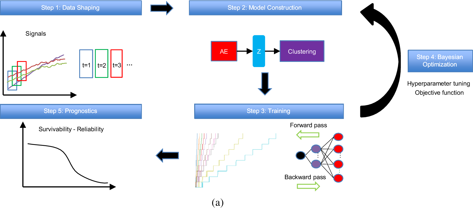


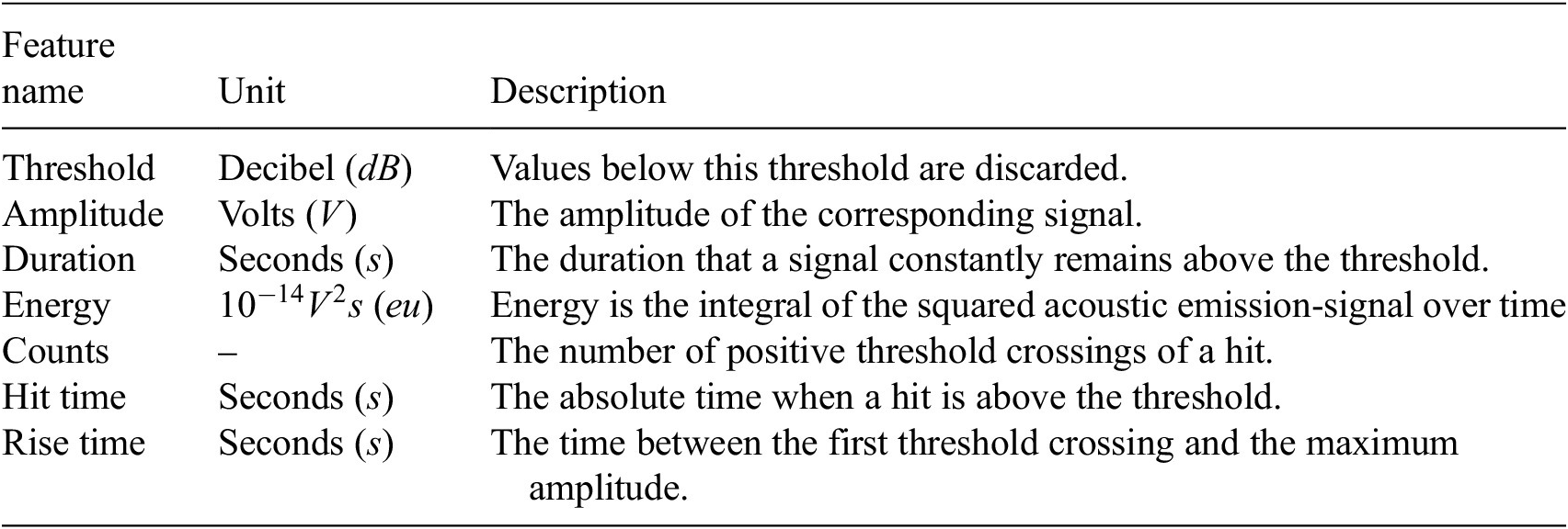
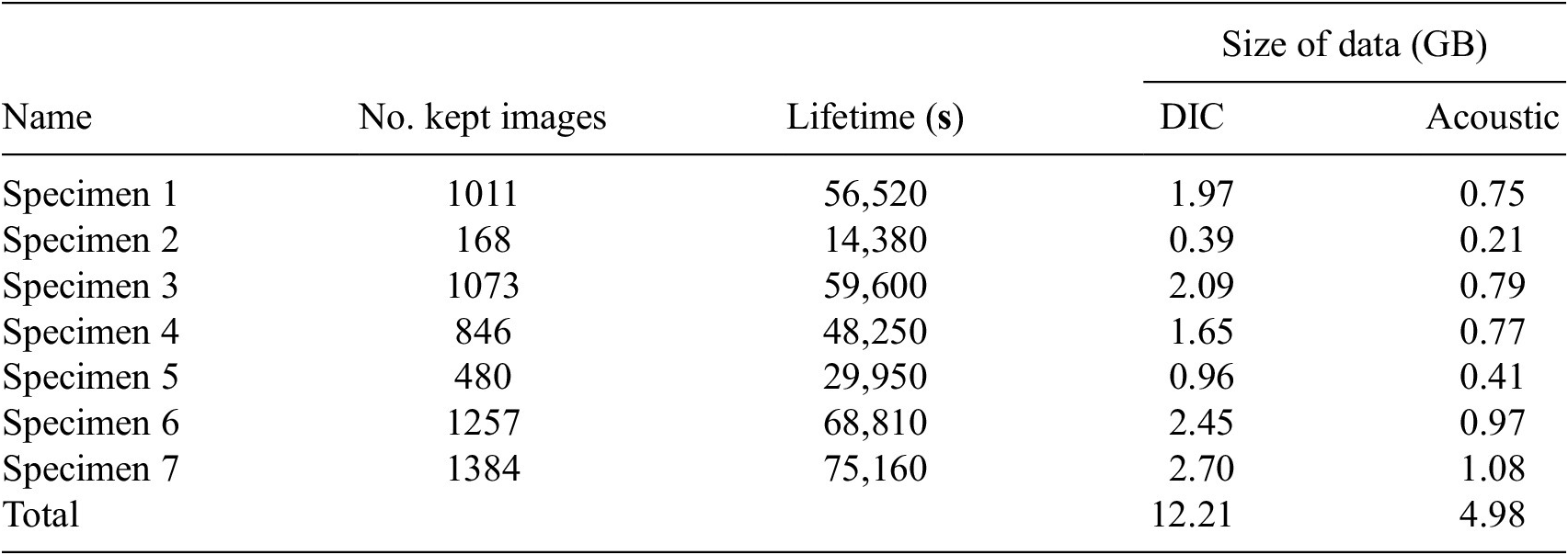
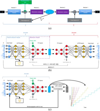

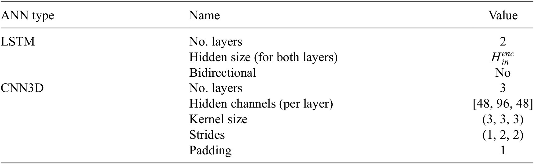
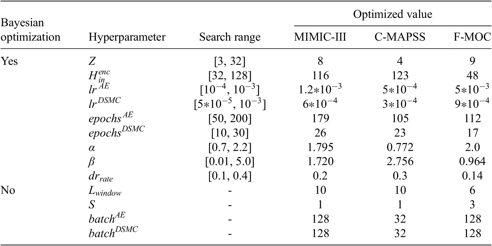
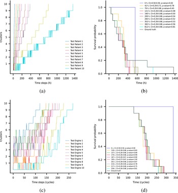
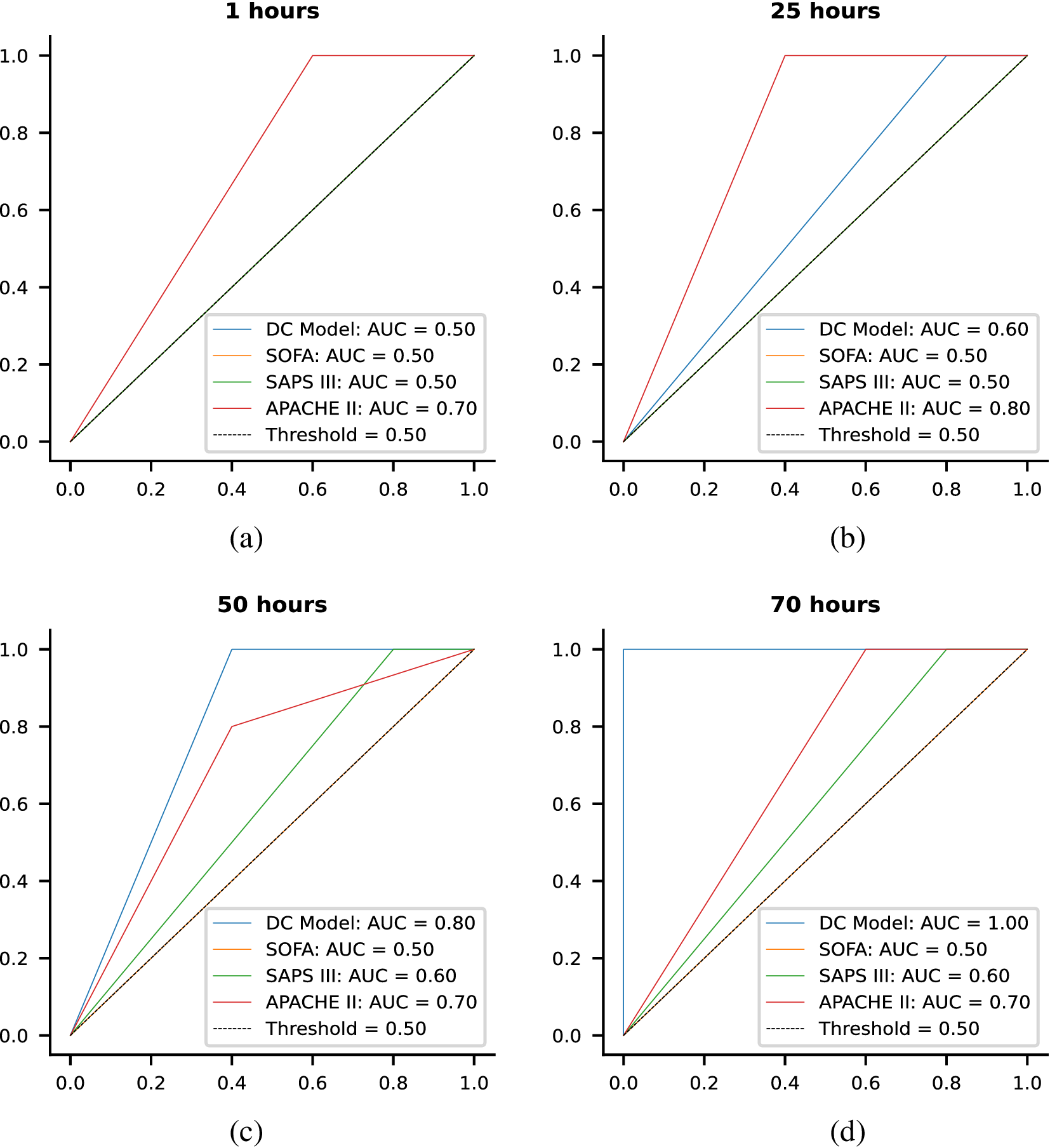
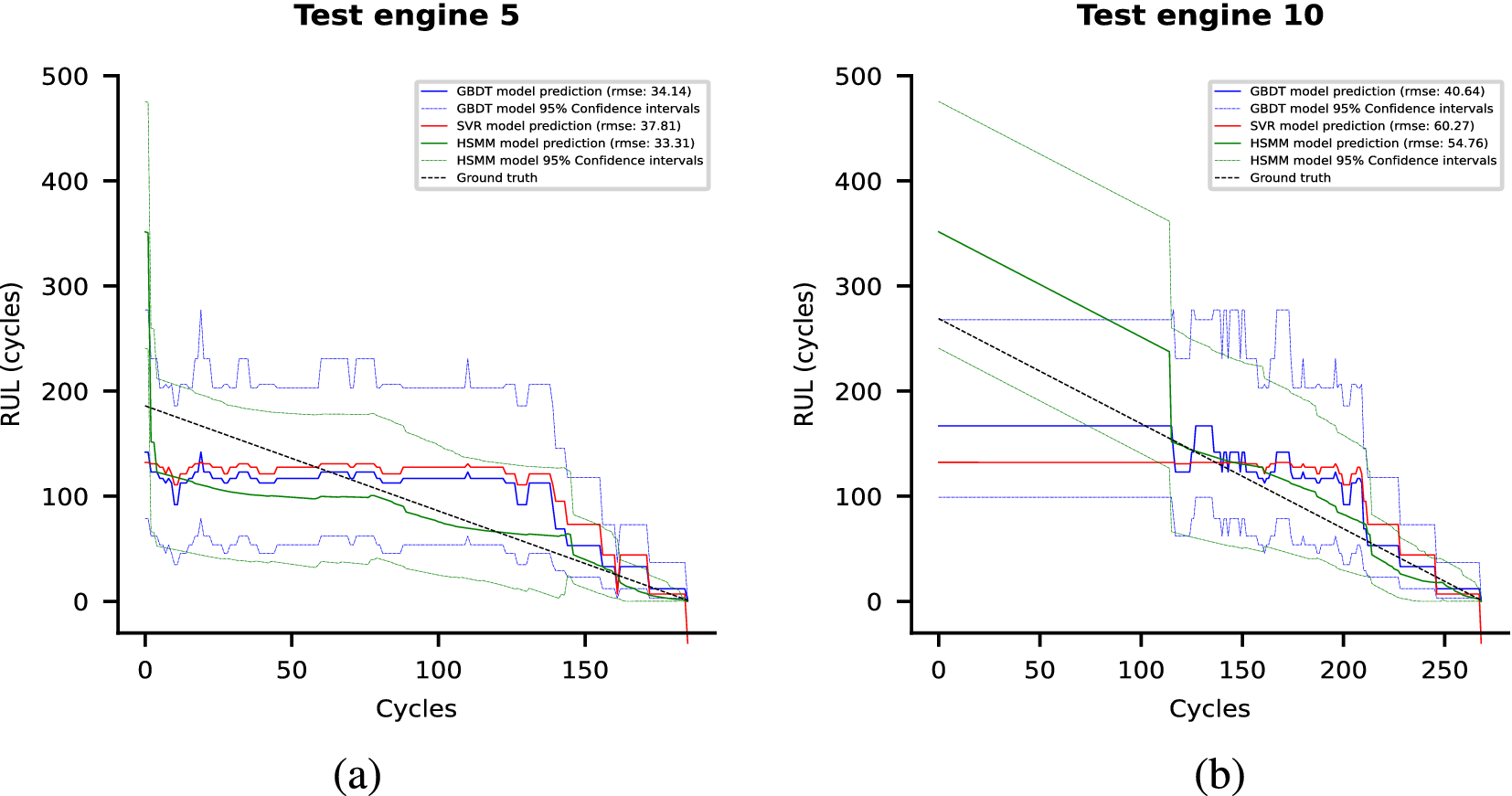
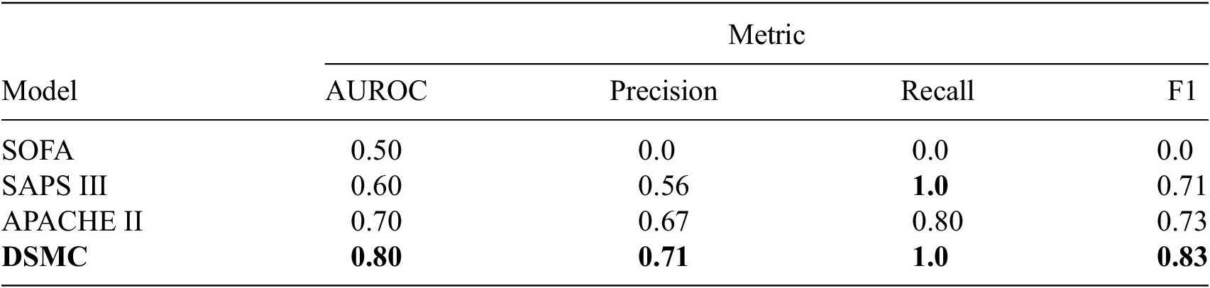

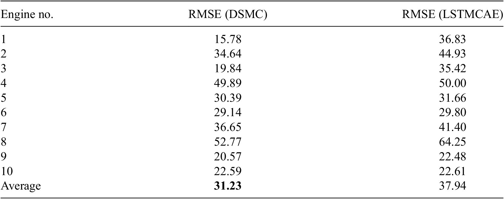
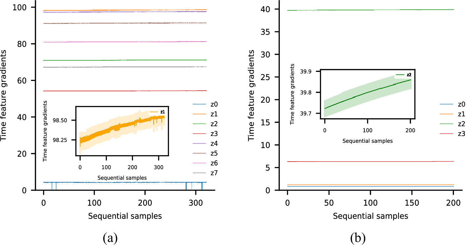


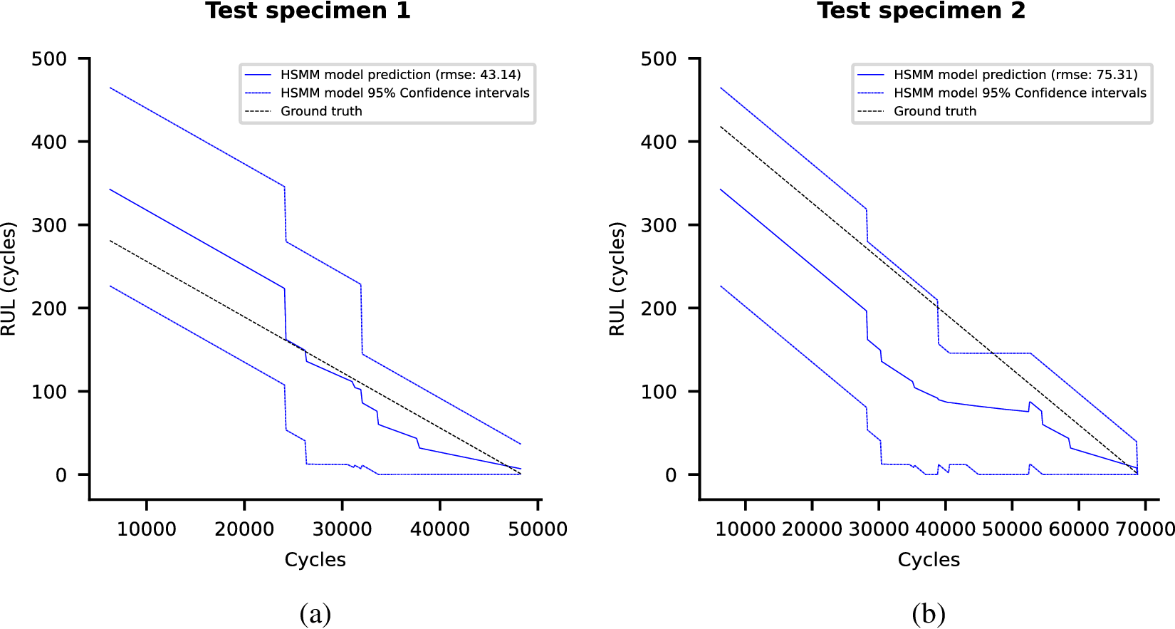
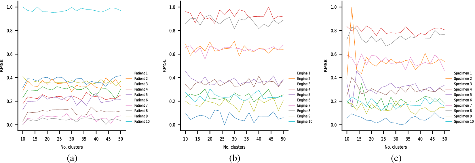

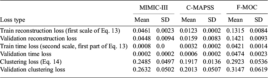

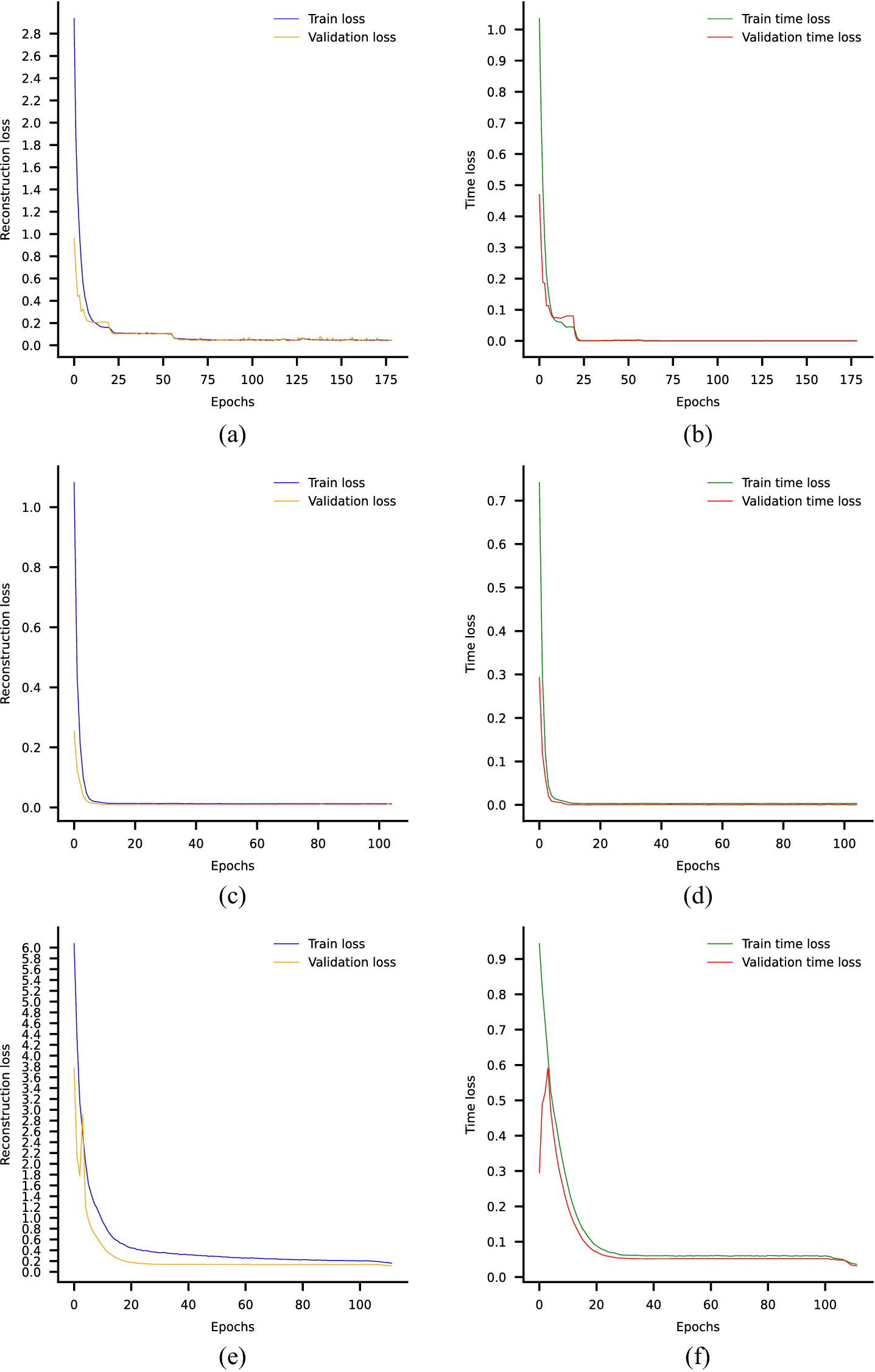

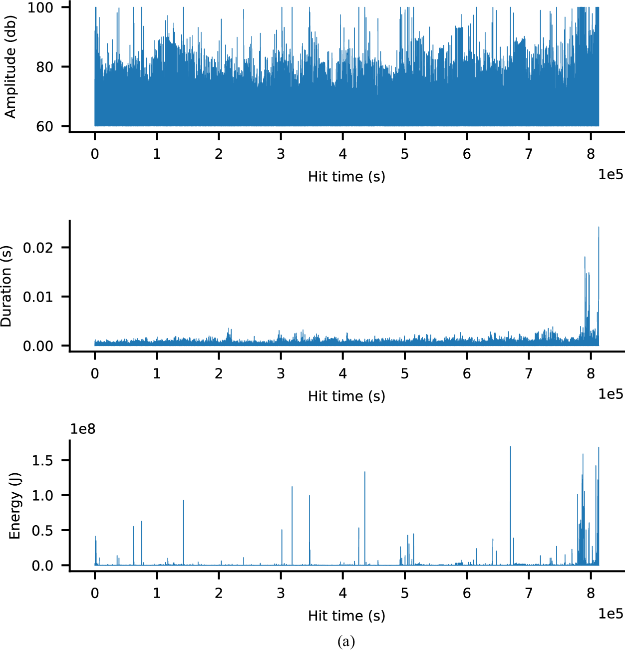


 Open access


Comments
No Comments have been published for this article.