

1. Introduction
Rapid progress in Natural Language Processing (NLP) has strongly influenced text classification tasks. After the introduction of the recent deep learning methods, many text classification benchmarks are either solved or close of being solved (Howard and Ruder Reference Howard and Ruder2018; Devlin et al. Reference Devlin, Chang, Lee and Toutanova2019; Radford et al. Reference Radford, Wu, Child, Luan, Amodei and Sutskever2019; Liu et al. Reference Liu, Ott, Goyal, Du, Joshi, Chen, Levy, Lewis, Zettlemoyer and Stoyanov2019b). By “solved,” we mean that the classification task can be performed by a computer with the same (or better) level of proficiency than humans. This phenomenon is exemplified by attempts of creating hard text categorization tasks like the GLUE and SuperGLUE datasets (Wang et al. Reference Wang, Singh, Michael, Hill, Levy and Bowman2018, Reference Wang, Pruksachatkun, Nangia, Singh, Michael, Hill, Levy and Bowman2019). Both datasets were created with the purpose of being robust datasets for language understanding. But just after a couple of years, both datasets have been surpassed by Transformer-based models (He et al. Reference He, Liu, Gao and Chen2020).
Natural Language Inference (NLI) is a classification task centered on deduction. In this task, a machine learning model determines the logical relationship between a pair of sentences $P$
and
$P$
and $H$
(referred to as premise and hypothesis, respectively). The model must assert that either that
$H$
(referred to as premise and hypothesis, respectively). The model must assert that either that $P$
entails
$P$
entails $H$
,
$H$
, $P$
, and
$P$
, and $H$
are in contradiction, or
$H$
are in contradiction, or $P$
and
$P$
and $H$
are neutral (logically independent) (Bowman et al. Reference Bowman, Angeli, Potts and Manning2015). Similar to other text classification tasks, NLI seems to be a solved problem. Computer performance has surpassed the human baseline in the traditional NLI datasets (SNLI and MNLI) (Bowman et al. Reference Bowman, Angeli, Potts and Manning2015; Williams, Nangia, and Bowman Reference Williams, Nangia and Bowman2018; Wang et al. Reference Wang, Singh, Michael, Hill, Levy and Bowman2022).
$H$
are neutral (logically independent) (Bowman et al. Reference Bowman, Angeli, Potts and Manning2015). Similar to other text classification tasks, NLI seems to be a solved problem. Computer performance has surpassed the human baseline in the traditional NLI datasets (SNLI and MNLI) (Bowman et al. Reference Bowman, Angeli, Potts and Manning2015; Williams, Nangia, and Bowman Reference Williams, Nangia and Bowman2018; Wang et al. Reference Wang, Singh, Michael, Hill, Levy and Bowman2022).
To challenge the inference capacity of the deep learning models, the NLI field has used adversarial techniques in different ways. A new wave of dynamic datasets adds humans and models during the data-collecting phase, transforming the static data acquisition process in an adversarial setting with multiple rounds. This process yields more challenging datasets that are far from being solved by deep learning models (Nie et al. Reference Nie, Williams, Dinan, Bansal, Weston and Kiela2020; Kiela et al. Reference Kiela, Bartolo, Nie, Kaushik, Geiger, Wu, Vidgen, Prasad, Singh, Ringshia, Ma, Thrush, Riedel, Waseem, Stenetorp, Jia, Bansal, Potts and Williams2021; Ma et al. Reference Ma, Ethayarajh, Thrush, Jain, Wu, Jia, Potts, Williams and Kiela2021).
Another line of work is a collection of adversarial evaluation schemes that propose different approaches, and, still, the core method is the same: define a new NLI set of examples (the adversarial set), train a model on a benchmark NLI dataset, and evaluate it on the adversarial examples (Glockner, Shwartz, and Goldberg Reference Glockner, Shwartz and Goldberg2018; Nie, Wang, and Bansal Reference Nie, Wang and Bansal2018; Dasgupta et al. Reference Dasgupta, Guo, Stuhlmüller, Gershman and Goodman2018; Zhu, Li, and de Melo Reference Zhu, Li and de Melo2018; Naik et al. Reference Naik, Ravichander, Sadeh, Rose and Neubig2018; McCoy, Pavlick, and Linzen Reference McCoy, Pavlick and Linzen2019; Yanaka et al. Reference Yanaka, Mineshima, Bekki, Inui, Sekine, Abzianidze and Bos2019; Liu, Schwartz, and Smith Reference Liu, Schwartz and Smith2019a; Richardson et al. Reference Richardson, Hu, Moss and Sabharwal2020). In all these papers, there is a significant drop in performance on the new test data. But, in almost all cases, this problem can be solved by using the appropriate training data. For example, Glockner et al. (Reference Glockner, Shwartz and Goldberg2018) observe that a statistical model is capable of learning synonym and antonym inference when sufficient examples were added in training.
The present article will address a methodological flaw in the adversarial evaluation literature. Instead of using adversarial test sets to highlight the limitations of the benchmark NLI datasets, we propose to use some adversarial techniques to investigate whether machine learning models, when trained with sufficient adversarial examples, can perform the same type of inference for different text inputs with the same intended meaning. For this purpose, we define a class of text transformations that can change a NLI input without altering the underlying logical relationship. Based on such transformations, we construct an experimental design where a percentage of the training data is substituted by its transformed version. We also define different versions of the test set: the original one obtained from a benchmark dataset, and the one where some observations are transformed. Then, we propose an adaptation of the paired t-test to compare the model’s performance on the two versions of the test set. We call the whole procedure the Invariance under Equivalence test (IE test). This approach provides two direct advantages: we substitute the expensive endeavor of dataset creation by the simpler task of constructing an adequate transformation function, and since the proposed hypothesis test is carefully crafted to account for the variety of ways that a transformation can affect the training of a machine learning model, we offer an evaluation procedure that is both meaningful and statistically sound.
As a case study, we examine the sensibility of different state-of-the-art models using the traditional NLI benchmarks Stanford Natural Language Inference Corpus (SNLI) (Bowman et al. Reference Bowman, Angeli, Potts and Manning2015) and MultiGenre NLI Corpus (MNLI) (Williams et al. Reference Williams, Nangia and Bowman2018) under a small perturbation based on synonym substitution. Two main results have been obtained:
-
Current deep learning models show two different inference outputs for sentences with the same meaning. After applying the IE test using both datasets and different percentages of transformation in the training data, we have observed that the deep learning models fail the IE test in the vast majority of cases. This result indicates that by just adding transformed examples in the fine-tuning phase we are not able to remove some biases originating in the pre-training stage.
-
Some NLI models are clearly more robust than others. By measuring each model’s performance on the non-transformed test set when altered examples are present in training, we have observed that BERT (Devlin et al. Reference Devlin, Chang, Lee and Toutanova2019) and RoBERTa (Liu et al. Reference Liu, Ott, Goyal, Du, Joshi, Chen, Levy, Lewis, Zettlemoyer and Stoyanov2019b) are significantly more robust than XLNet (Yang et al. Reference Yang, Dai, Yang, Carbonell, Salakhutdinov and Le2019) and ALBERT (Lan et al. Reference Lan, Chen, Goodman, Gimpel, Sharma and Soricut2020).
The article is organized as follows: in Section 2 we show how to define logical preserving transformations using the notion of equivalence; in Section 3 we introduce the IE test; in Sections 4 and 5, we present one application of the IE test for the case of synonym substitution and comment on the experimental results; in Section 6, we discuss the related literature, and, finally, in Section 7, we address open issues and future steps.
2. Equivalence
The concept of equivalence, which is formally defined in logic, can also be employed in natural language with some adjustments to take into account its complex semantics. Once we establish an equivalent relation, we define a function that maps sentences to their equivalent counterpart and extend this function to any NLI dataset.
2.1. Equivalence in formal and natural languages
In formal logic, we say that two formulas are equivalent if both have the same truth value. For example, let $\boldsymbol{{p}}$
denote a propositional variable,
$\boldsymbol{{p}}$
denote a propositional variable, $\land$
the conjunction operator, and
$\land$
the conjunction operator, and $\top$
a tautology (a sentence which is always true, e.g.,
$\top$
a tautology (a sentence which is always true, e.g., $0=0$
). The truth value of the formula
$0=0$
). The truth value of the formula $\boldsymbol{{p}}\land \top$
depends only on
$\boldsymbol{{p}}\land \top$
depends only on $\boldsymbol{{p}}$
(in general, any formula of the form
$\boldsymbol{{p}}$
(in general, any formula of the form $\boldsymbol{{p}}\land \top \land \ldots \land \top$
has the same truth value as
$\boldsymbol{{p}}\land \top \land \ldots \land \top$
has the same truth value as $\boldsymbol{{p}}$
). Hence, we say that
$\boldsymbol{{p}}$
). Hence, we say that $\boldsymbol{{p}}\land \top$
and
$\boldsymbol{{p}}\land \top$
and $\boldsymbol{{p}}$
are equivalent formulas.
$\boldsymbol{{p}}$
are equivalent formulas.
Together with a formal language, we also define a deductive system, a collection of transformation rules that govern how to derive one formula from a set of premises. By $\Gamma \vdash \boldsymbol{{p}}$
, we mean that the formula
$\Gamma \vdash \boldsymbol{{p}}$
, we mean that the formula $\boldsymbol{{p}}$
is derivable in the system when we use the set of formulas
$\boldsymbol{{p}}$
is derivable in the system when we use the set of formulas $\Gamma$
as premises. Often we want to define a complete system, that is a system where the formulas derived without any premises are exactly the ones that are true.
$\Gamma$
as premises. Often we want to define a complete system, that is a system where the formulas derived without any premises are exactly the ones that are true.
In a complete system, we can substitute one formula for any of its equivalent versions without disrupting the derivations from the system. This simply means that, under a complete system, equivalent formulas derive the same facts. For example, let $\boldsymbol{{q}}$
be a propositional variable, and
$\boldsymbol{{q}}$
be a propositional variable, and $\rightarrow$
is the implication connective. It follows that
$\rightarrow$
is the implication connective. It follows that
 \begin{equation} \big\{\boldsymbol{{p}}, \boldsymbol{{p}}\rightarrow \boldsymbol{{q}} \big\} \vdash \boldsymbol{{q}}, \qquad \text{ and } \qquad \big\{\boldsymbol{{p}} \land \top, \boldsymbol{{p}}\rightarrow \boldsymbol{{q}} \big\} \vdash \boldsymbol{{q}} \land \top. \end{equation}
The main point in Expression (1) is that, under a complete system, if we take $\boldsymbol{{p}}\rightarrow \boldsymbol{{q}}$
and any formula equivalent to
$\boldsymbol{{p}}\rightarrow \boldsymbol{{q}}$
and any formula equivalent to $\boldsymbol{{p}}$
as premises, the system always derives a formula equivalent to
$\boldsymbol{{p}}$
as premises, the system always derives a formula equivalent to $\boldsymbol{{q}}$
. This result offers one simple way to verify that a system is incomplete: we can take an arbitrary pair of equivalent formulas and check whether by substituting one for the other the system’s deductions diverge.
$\boldsymbol{{q}}$
. This result offers one simple way to verify that a system is incomplete: we can take an arbitrary pair of equivalent formulas and check whether by substituting one for the other the system’s deductions diverge.
We propose to incorporate this verification procedure to the NLI field. This is a feasible approach because the concept of equivalence can be understood in natural language as meaning identity (Shieber Reference Shieber1993). Thus, we formulate the property associated with a complete deductive system as a linguistic competence:
If two sentences have the same meaning, it is expected that any consequence based on them should not be disrupted when we substitute one sentence for the other.
We call this competence the invariance under equivalence (IE) property. Similar to formal logic, we can investigate the limitations of NLI models by testing if they fail to satisfy the IE property. In this type of investigation, we assess whether a machine leaning model produces the same classification when faced with two equivalent texts. And to produce equivalent versions of the same textual input, we employ meaning preserving textual transformations.
2.2. Equivalences versus destructive transformations
In NLP, practitioners use “adversarial examples” to denote a broad set of text transformations. Such examples can refer to some textual transformations constructed to disrupt the original meaning of a sentence (Naik et al. Reference Naik, Ravichander, Sadeh, Rose and Neubig2018; Nie et al. Reference Nie, Wang and Bansal2018; Liu et al. Reference Liu, Schwartz and Smith2019a). However, some modifications can transform the original sentence, making it completely lose its original meaning. Researchers may employ such destructive transformations to check whether a model uses some specific linguistic aspect while solving an NLP task. For example, Naik et al. (Reference Naik, Ravichander, Sadeh, Rose and Neubig2018) aimed at testing whether machine learning models are heavily dependent on word-level information, and defined a transformation that swaps the subject and object appearing in a sentence. Sinha et al. (Reference Sinha, Parthasarathi, Pineau and Williams2021) presented another relevant work in that line, in which, after transforming sentences by a word reordering process, showed that transformer-based models are insensitive to syntax-destroying transformations. And more recently, Talman et al. (Reference Talman, Apidianaki, Chatzikyriakidis and Tiedemann2021) applied a series of corruption transformations to NLI datasets to check the quality of those data.
Unlike the works mentioned above, the present article focuses only on the subset of textual transformations designed not to disturb the underlying logical relationship in an NLI example (what we refer to as “equivalences”). Note that there is no one-to-one relationship between logical equivalence and meaning identity. Some pragmatics and commonsense reasoning are obstructed when we perform text modification. For example, two expressions can denote the same object, but one expression is embedded in a specific context. One well-known example is the term “the morning star,” referring to the planet Venus. Although both terms refer to the same celestial object, any scientific-minded person will find it strange when one replaces Venus with the morning star in the sentence Venus is the second planet from the Sun. Such discussions are relevant, but we will deliberately ignore them here. We focus on text transformations that can preserve meaning identity and can be implemented in an automatic process. Hence, as a compromise, we will allow text transformations that derange the pragmatic aspects of the sentence.
So far, we have spoken about equivalent transformations in a general way. It is worthwhile to offer some concrete examples:
Synonym substitution: the primary case of equivalence can be found in sentences composed of constituents with the same denotation. For example, take the sentences: a man is fishing, and a guy is fishing. This instance shows the case where one sentence can be obtained from the other by replacing one or more words with their respective synonyms while denoting the same fact.
Constituents permutation: since many relations in natural language are symmetric, we can permute the relations’ constituents without causing meaning disruption. This can be done using either definite descriptions or relative clauses. In the case of definite descriptions, we can freely permute the entity being described and the description. For example, Iggy Pop was the lead singer of the Stooges is equivalent to The lead singer of the Stooges was Iggy Pop. When using relative clauses, the phrases connected can be rearranged in any order. For example, John threw a red ball that is large is interchangeable with John threw a large ball that is red.
Voice transformation: one stylistic transformation that is usually performed in writing is the change in grammatical voice. It is possible to write different sentences both in the active and passive voice: the crusaders captured the holy city can be modified to the holy city was captured by the crusaders, and vice-versa.
In the next section, we will assume that there is a transformation function $\varphi$
that map sentences to an equivalent form. For example,
$\varphi$
that map sentences to an equivalent form. For example, $\varphi$
could be a voice transformation function:
$\varphi$
could be a voice transformation function:
- $P =$
Galileo discovered Jupiter’s four largest moons.
$P =$
Galileo discovered Jupiter’s four largest moons. -
$P^\varphi =$
Jupiter’s four largest moons were discovered by Galileo.


3. Testing for invariance
In this section, we propose an experimental design to measure the IE property for the NLI task: the IE test. Broadly speaking, the IE test is composed of three main steps: (i) we resample an altered version of the training data and obtain a classifier by estimating the model’s parameters on the transformed sample; (ii) we perform a paired t-test to compare the classifier’s performance on the two versions of the test set; (iii) we repeat steps (i) and (ii) $M$
times and employ the Bonferroni method (Wasserman Reference Wasserman2010) to combine the multiple paired t-tests into a single decision procedure. In what follows, we describe in detail steps (i), (ii), and (iii). After establishing all definitions, we present the IE test as an algorithm and comment on some alternatives.
$M$
times and employ the Bonferroni method (Wasserman Reference Wasserman2010) to combine the multiple paired t-tests into a single decision procedure. In what follows, we describe in detail steps (i), (ii), and (iii). After establishing all definitions, we present the IE test as an algorithm and comment on some alternatives.
3.1. Training on a transformed sample
First, let us define a generation process to model the different effects caused by the presence of a transformation function on the training stage. Since we are assuming that any training observation can be altered, the generation method is constructed as a stochastic process.
Given a transformation $\varphi$
and a transformation probability
$\varphi$
and a transformation probability $\rho \in [0,1]$
we define the
$\rho \in [0,1]$
we define the $(\varphi, \rho )$
data-generating process, DGP
$(\varphi, \rho )$
data-generating process, DGP $_{\varphi, \rho }(\mathcal{D}_{{T}}, \mathcal{D}_{{V}})$
, as the process of obtaining a modified version of the train and validation datasets where the probability of each observation being altered by
$_{\varphi, \rho }(\mathcal{D}_{{T}}, \mathcal{D}_{{V}})$
, as the process of obtaining a modified version of the train and validation datasets where the probability of each observation being altered by $\varphi$
is
$\varphi$
is $\rho$
. More precisely, let
$\rho$
. More precisely, let $\mathcal{D}_{{}} \in \{\mathcal{D}_{{T}}, \mathcal{D}_{{V}}\}$
be one of the datasets and denote its length by
$\mathcal{D}_{{}} \in \{\mathcal{D}_{{T}}, \mathcal{D}_{{V}}\}$
be one of the datasets and denote its length by $|\mathcal{D}_{{}}|= n$
. Also, consider the following selection variables
$|\mathcal{D}_{{}}|= n$
. Also, consider the following selection variables $L_1, \ldots, L_n \thicksim \text{Bernoulli}(\rho )$
. An altered version of
$L_1, \ldots, L_n \thicksim \text{Bernoulli}(\rho )$
. An altered version of $\mathcal{D}_{{}}$
is the set composed of the observations of the form
$\mathcal{D}_{{}}$
is the set composed of the observations of the form $({P_i}^{new},{H_i}^{new},Y_i)$
, where:
$({P_i}^{new},{H_i}^{new},Y_i)$
, where:
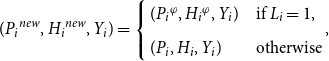 \begin{align} ({P_i}^{{new}},{H_i}^{{new}}, Y_i) = \left\{ \begin{array}{l@{\quad}l} ({P_i}^{\varphi },{H_i}^{\varphi }, Y_i) & \textrm{if } L_i = 1, \\[3pt] (P_i, H_i, Y_i) & \textrm{otherwise} \end{array},\right. \end{align}
and $Y_i$
is the
$Y_i$
is the $i$
th label associated with the NLI input
$i$
th label associated with the NLI input $(P_i, H_i)$
. This process is applied independently to
$(P_i, H_i)$
. This process is applied independently to $\mathcal{D}_{{T}}$
and
$\mathcal{D}_{{T}}$
and $\mathcal{D}_{{V}}$
. Hence, if
$\mathcal{D}_{{V}}$
. Hence, if $|\mathcal{D}_{{T}}|= n_1$
and
$|\mathcal{D}_{{T}}|= n_1$
and $|\mathcal{D}_{{V}}|= n_2$
, then there are
$|\mathcal{D}_{{V}}|= n_2$
, then there are $2^{(n_1 + n_2)}$
distinct pairs of transformed sets
$2^{(n_1 + n_2)}$
distinct pairs of transformed sets $({\mathcal{D}_{{T}}}^{\prime },{\mathcal{D}_{{V}}}^{\prime })$
that can be sampled. We write
$({\mathcal{D}_{{T}}}^{\prime },{\mathcal{D}_{{V}}}^{\prime })$
that can be sampled. We write
 \begin{equation}{\mathcal{D}_{{T}}}^{\prime },{\mathcal{D}_{{V}}}^{\prime } \thicksim \text{ DGP}_{\varphi, \rho }(\mathcal{D}_{{T}}, \mathcal{D}_{{V}}) \end{equation}
to denote the process of sampling a transformed version of the datasets $\mathcal{D}_{{T}}$
and
$\mathcal{D}_{{T}}$
and $\mathcal{D}_{{V}}$
according to
$\mathcal{D}_{{V}}$
according to $\varphi$
and
$\varphi$
and $\rho$
.
$\rho$
.
Second, to represent the whole training procedure we need to define the underlying NLI model and the hyperparameter space. For $d,s\in \mathbb{N}$
, let
$d,s\in \mathbb{N}$
, let $\mathcal{M} = \{ f(x;\ \theta ) \;:\; \theta \in \Theta \subseteq \mathbb{R}^{{d}}\}$
be a parametric model, and let
$\mathcal{M} = \{ f(x;\ \theta ) \;:\; \theta \in \Theta \subseteq \mathbb{R}^{{d}}\}$
be a parametric model, and let $\mathcal{H}_{\mathcal{M}} \subseteq \mathbb{R}^{{s}}$
be the associated hyperparameters space, where
$\mathcal{H}_{\mathcal{M}} \subseteq \mathbb{R}^{{s}}$
be the associated hyperparameters space, where $s$
is the number of hyperparameters, required by the model. By search, we denote any algorithm of hyperparameter selection, for example random search (Bergstra and Bengio Reference Bergstra and Bengio2012). Thus, given a number of maximum search
$s$
is the number of hyperparameters, required by the model. By search, we denote any algorithm of hyperparameter selection, for example random search (Bergstra and Bengio Reference Bergstra and Bengio2012). Thus, given a number of maximum search $\mathcal{B}$
, a budget, this algorithm chooses a specific hyperparameter value
$\mathcal{B}$
, a budget, this algorithm chooses a specific hyperparameter value $h \in \mathcal{H}_{\mathcal{M}}$
:
$h \in \mathcal{H}_{\mathcal{M}}$
:
 \begin{equation} h = \text{search}(\mathcal{D}_{{T}}, \mathcal{D}_{{V}}, \mathcal{M}, \mathcal{H}_{\mathcal{M}}, \mathcal{B}). \end{equation}
A classifier $g$
is attained by fitting the model
$g$
is attained by fitting the model $\mathcal{M}$
on the training data
$\mathcal{M}$
on the training data $({\mathcal{D}_{{T}}}^{\prime },{\mathcal{D}_{{V}}}^{\prime })$
based on a hyperparameter value
$({\mathcal{D}_{{T}}}^{\prime },{\mathcal{D}_{{V}}}^{\prime })$
based on a hyperparameter value $h$
and a stochastic approximation algorithm (train):
$h$
and a stochastic approximation algorithm (train):
 \begin{equation} g = \text{train}(\mathcal{M},{\mathcal{D}_{{T}}}^{\prime },{\mathcal{D}_{{V}}}^{\prime }, h). \end{equation}
The function $g$
is a usual NLI classifier: its input is the pair of sentences
$g$
is a usual NLI classifier: its input is the pair of sentences $(P,H)$
, and its output is either
$(P,H)$
, and its output is either $-1$
(contradiction),
$-1$
(contradiction), $0$
(neutral), or
$0$
(neutral), or $1$
(entailment).
$1$
(entailment).
3.2. A bootstrap version of the paired t-test
Let $\mathcal{D}_{{Te}}$
be the test dataset, and let
$\mathcal{D}_{{Te}}$
be the test dataset, and let $\mathcal{D}_{{Te}}^{\varphi }$
be the version of this dataset where all observations are altered by
$\mathcal{D}_{{Te}}^{\varphi }$
be the version of this dataset where all observations are altered by $\varphi$
. The IE test is based on the comparison of the classifier’s accuracies in two paired samples:
$\varphi$
. The IE test is based on the comparison of the classifier’s accuracies in two paired samples: $\mathcal{D}_{{Te}}$
and
$\mathcal{D}_{{Te}}$
and $\mathcal{D}_{{Te}}^{\varphi }$
. Pairing occurs because each member of a sample is matched with an equivalent member in the other sample. To account for this dependency, we perform a paired t-test. Since we cannot guarantee that the presuppositions of asymptotic theory are preserved in this context, we formulate the paired t-test as a bootstrap hypothesis test (Fisher and Hall Reference Fisher and Hall1990; Konietschke and Pauly Reference Konietschke and Pauly2014).
$\mathcal{D}_{{Te}}^{\varphi }$
. Pairing occurs because each member of a sample is matched with an equivalent member in the other sample. To account for this dependency, we perform a paired t-test. Since we cannot guarantee that the presuppositions of asymptotic theory are preserved in this context, we formulate the paired t-test as a bootstrap hypothesis test (Fisher and Hall Reference Fisher and Hall1990; Konietschke and Pauly Reference Konietschke and Pauly2014).
Given a classifier $g$
, let
$g$
, let $A$
and
$A$
and $B$
be the variables indicating the correct classification of the two types of random NLI observation:
$B$
be the variables indicating the correct classification of the two types of random NLI observation:
 \begin{equation} A = I(g(P, H) = Y), \qquad B = I(g({P}^{\varphi },{H}^{\varphi }) = Y), \end{equation}
where $I$
is the indicator function, and
$I$
is the indicator function, and $Y$
is either
$Y$
is either $-1$
(contradiction),
$-1$
(contradiction), $0$
(neutral), or
$0$
(neutral), or $1$
(entailment). The true accuracy of
$1$
(entailment). The true accuracy of $g$
for both versions of the text input is given by
$g$
for both versions of the text input is given by
 \begin{equation}{\mathbb{E}}[A] ={\mathbb{P}}(g(P, H) = Y), \qquad{\mathbb{E}}[B] ={\mathbb{P}}(g({P}^{\varphi },{H}^{\varphi }) = Y). \end{equation}
We approximate these quantities by using the estimators $\bar{A}$
and
$\bar{A}$
and $\bar{B}$
defined on the test data
$\bar{B}$
defined on the test data $\mathcal{D}_{{Te}} = \{ (P_i, H_i, Y_i) \; : \; i =1, \ldots, n \}$
:
$\mathcal{D}_{{Te}} = \{ (P_i, H_i, Y_i) \; : \; i =1, \ldots, n \}$
:
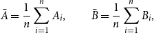 \begin{equation} \bar{A} = \frac{1}{n}\sum _{i=1}^{n}A_i, \qquad \bar{B} = \frac{1}{n}\sum _{i=1}^{n}B_i, \end{equation}
where $A_i$
and
$A_i$
and $B_i$
indicate the classifier’s correct prediction on the original and altered version of the
$B_i$
indicate the classifier’s correct prediction on the original and altered version of the $i$
th observation, respectively. Let match be the function that returns the vector of matched observations related to the performance of
$i$
th observation, respectively. Let match be the function that returns the vector of matched observations related to the performance of $g$
on the datasets
$g$
on the datasets $\mathcal{D}_{{Te}}$
and
$\mathcal{D}_{{Te}}$
and $\mathcal{D}_{{Te}}^{\varphi }$
:
$\mathcal{D}_{{Te}}^{\varphi }$
:
 \begin{align} \text{match}(g, \mathcal{D}_{{Te}}, \mathcal{D}_{{Te}}^{\varphi }) & = ((A_1,B_1), \ldots, (A_n,B_n)) & \mbox{(matched sample)}. \end{align}
In the matched sample (Equation 9), we have information about the classifier’s behavior for each observation of the test data before and after applying the transformation $\varphi$
. Let
$\varphi$
. Let $\delta$
be defined as the difference between probabilities:
$\delta$
be defined as the difference between probabilities:
 \begin{equation} \delta ={\mathbb{E}}[A] -{\mathbb{E}}[B]. \end{equation}
We test hypothesis $H_0$
that the probabilities are equal against hypothesis
$H_0$
that the probabilities are equal against hypothesis $H_1$
that they are different:
$H_1$
that they are different:
 \begin{equation} H_0\,:\, \delta = 0 \text{ versus } H_1\,:\, \delta \neq 0. \end{equation}
Let $\hat{\delta }_i = A_i - B_i$
and
$\hat{\delta }_i = A_i - B_i$
and $\hat{\delta } = \bar{A} - \bar{B}$
. We test
$\hat{\delta } = \bar{A} - \bar{B}$
. We test $H_0$
by using the paired t-test statistic:
$H_0$
by using the paired t-test statistic:
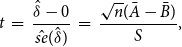 \begin{equation} t \;=\; \frac{\hat{\delta } - 0}{\hat{se}(\hat{\delta })} \;=\; \frac{\sqrt{n}(\bar{A} - \bar{B})}{S}, \end{equation}
such that $\hat{se}(\hat{\delta }) = S / \sqrt{n}$
is the estimated standard error of
$\hat{se}(\hat{\delta }) = S / \sqrt{n}$
is the estimated standard error of $\hat{\delta }$
, where
$\hat{\delta }$
, where
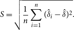 \begin{equation} S = \sqrt{\frac{1}{n}\sum _{i=1}^{n}(\hat{\delta }_i - \hat{\delta })^2}. \end{equation}
In order to formulate the IE test in a suitable manner, we write $X = (X_1, \ldots, X_n)$
to denote the vector of paired variables (Equation 9), that is
$X = (X_1, \ldots, X_n)$
to denote the vector of paired variables (Equation 9), that is $X_i = (A_i, B_i)$
for
$X_i = (A_i, B_i)$
for $i \in \{1, \ldots, n\}$
. We also use
$i \in \{1, \ldots, n\}$
. We also use $t=f_{\text{paired t-test}}(X)$
to refer to the process of obtaining the test statistic (Equation 12) based on the matched data
$t=f_{\text{paired t-test}}(X)$
to refer to the process of obtaining the test statistic (Equation 12) based on the matched data $X$
. The observable test statistic is denoted by
$X$
. The observable test statistic is denoted by $\hat{t}$
.
$\hat{t}$
.
The test statistic $t$
is a standardized version of the accuracy difference
$t$
is a standardized version of the accuracy difference $\bar{A} - \bar{B}$
. A positive value for
$\bar{A} - \bar{B}$
. A positive value for $t$
implies that
$t$
implies that $\bar{A} \gt \bar{B}$
(the classifier is performing better on the original data compared to the transformed data). Similarly, when
$\bar{A} \gt \bar{B}$
(the classifier is performing better on the original data compared to the transformed data). Similarly, when $t$
takes negative values we have that
$t$
takes negative values we have that $\bar{B} \gt \bar{A}$
(the performance on the modified test data surpasses the performance on the original test set).
$\bar{B} \gt \bar{A}$
(the performance on the modified test data surpasses the performance on the original test set).
According to statistical theory of hypothesis testing, if the null hypothesis ( $H_0$
) is true, then it is more likely that the observed value
$H_0$
) is true, then it is more likely that the observed value $\hat{t}$
takes values closer to zero. But we need a probability distribution to formulate probability judgments about
$\hat{t}$
takes values closer to zero. But we need a probability distribution to formulate probability judgments about $\hat{t}$
.
$\hat{t}$
.
If the dependency lies only between each pair of variables $A_i$
and
$A_i$
and $B_i$
, then
$B_i$
, then $(A_1,B_1), \ldots, (A_n,B_n)$
is a sequence of indepent tuples. And so,
$(A_1,B_1), \ldots, (A_n,B_n)$
is a sequence of indepent tuples. And so, $\hat{\delta }_1, \ldots, \hat{\delta }_n$
are
$\hat{\delta }_1, \ldots, \hat{\delta }_n$
are $n$
independent and identically distributed (IID) data points. Moreover, if we assume the null hypothesis (
$n$
independent and identically distributed (IID) data points. Moreover, if we assume the null hypothesis ( $H_0$
), we have that
$H_0$
), we have that ${\mathbb{E}}[\delta ]={\mathbb{E}}[A] -{\mathbb{E}}[B] = 0$
. By a version of the Central Limit Theorem (Wasserman Reference Wasserman2010, Theorem 5.10),
${\mathbb{E}}[\delta ]={\mathbb{E}}[A] -{\mathbb{E}}[B] = 0$
. By a version of the Central Limit Theorem (Wasserman Reference Wasserman2010, Theorem 5.10), $t$
converges (in distribution) to a standard normal distribution and, therefore, we can use this normal distribution to make approximate inferences about
$t$
converges (in distribution) to a standard normal distribution and, therefore, we can use this normal distribution to make approximate inferences about $\hat{t}$
under
$\hat{t}$
under $H_0$
.
$H_0$
.
However, it is well-documented in the NLI literature that datasets created through crowdsourcing (like the SNLI and MNLI datasets) present annotator bias: multiple observations can have a dependency between them due to the language pattern of some annotators (Gururangan et al. Reference Gururangan, Swayamdipta, Levy, Schwartz, Bowman and Smith2018; Geva, Goldberg, and Berant Reference Geva, Goldberg and Berant2019). Thus, in the particular setting of NLI, it is naive to assume that the data are IID and apply the Central Limit Theorem. One alternative method provided by statistics is using the bootstrapping sampling strategy (Fisher and Hall Reference Fisher and Hall1990).
Following the bootstrap method, we estimate the distribution of $t$
under the null hypothesis through resampling the matched data (Equation 9). It is worth noting that we need to generate observations under
$t$
under the null hypothesis through resampling the matched data (Equation 9). It is worth noting that we need to generate observations under $H_0$
from the observed sample, even when the observed sample is drawn from a population that does not satisfy
$H_0$
from the observed sample, even when the observed sample is drawn from a population that does not satisfy $H_0$
. In the case of the paired t-test, we employ the resampling strategy mentioned by Konietschke and Pauly (Reference Konietschke and Pauly2014): a resample
$H_0$
. In the case of the paired t-test, we employ the resampling strategy mentioned by Konietschke and Pauly (Reference Konietschke and Pauly2014): a resample $X^{*} = (X^*_1, \ldots, X^*_n)$
is drawn from the original sample with replacement such that each
$X^{*} = (X^*_1, \ldots, X^*_n)$
is drawn from the original sample with replacement such that each $X^*_i$
is a random permutation on the variables
$X^*_i$
is a random permutation on the variables $A_j$
and
$A_j$
and $B_j$
within the pair
$B_j$
within the pair $(A_j, B_j)$
for
$(A_j, B_j)$
for $j \in \{1,\ldots, n\}$
. In other words,
$j \in \{1,\ldots, n\}$
. In other words, $X^{*}$
is a normal bootstrap sample with the addition that each simulated variable
$X^{*}$
is a normal bootstrap sample with the addition that each simulated variable $X^*_i$
is either
$X^*_i$
is either $(A_j, B_j)$
or
$(A_j, B_j)$
or $(B_j, A_j)$
, with probability
$(B_j, A_j)$
, with probability $1/2$
, for some
$1/2$
, for some $j \in \{1,\ldots, n\}$
. This is done to force that the average values related to the first and second components are the same, following the null hypothesis (in this case,
$j \in \{1,\ldots, n\}$
. This is done to force that the average values related to the first and second components are the same, following the null hypothesis (in this case, ${\mathbb{E}}[A] ={\mathbb{E}}[B]$
).
${\mathbb{E}}[A] ={\mathbb{E}}[B]$
).
We use the simulated sample $X^{*}$
to calculate the bootstrap replication of
$X^{*}$
to calculate the bootstrap replication of $t$
,
$t$
, $t^* = f_{\text{paired t-test}}(X^*)$
. By repeating this process
$t^* = f_{\text{paired t-test}}(X^*)$
. By repeating this process $\mathcal{S}$
times, we obtain a collection of bootstrap replications
$\mathcal{S}$
times, we obtain a collection of bootstrap replications $t^*_1, \ldots, t^*_{\mathcal{S}}$
. Let
$t^*_1, \ldots, t^*_{\mathcal{S}}$
. Let $\hat{F}^*$
be the empirical distribution of
$\hat{F}^*$
be the empirical distribution of $t^*_s$
. We compute the equal-tail bootstrap p-value as follows:
$t^*_s$
. We compute the equal-tail bootstrap p-value as follows:
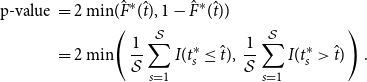 \begin{align} \text{p-value } &= 2 \min\!(\hat{F}^*(\hat{t}), 1- \hat{F}^*(\hat{t}))\nonumber \\ & = 2 \min\!\left (\, \frac{1}{\mathcal{S}}\sum _{s=1}^{\mathcal{S}}I(t^*_s \leq \hat{t}),\; \frac{1}{\mathcal{S}}\sum _{s=1}^{\mathcal{S}}I(t^*_s \gt \hat{t})\,\right ). \end{align}
In (14), we are simultaneously performing a left-tailed and a right-tailed test. The p-value is the probability of observing a bootstrap replication, in absolute value $|t^*|$
, larger than the actual observed statistic, in absolute value
$|t^*|$
, larger than the actual observed statistic, in absolute value $|\hat{t}|$
, under the null hypothesis.Footnote
a
$|\hat{t}|$
, under the null hypothesis.Footnote
a
3.3. Multiple testing
We make use of the $(\varphi, \rho )$
data-generating process to produce different effects caused by the presence of
$(\varphi, \rho )$
data-generating process to produce different effects caused by the presence of $\varphi$
in the training stage. This process results in a variety of classifiers influenced by
$\varphi$
in the training stage. This process results in a variety of classifiers influenced by $\varphi$
in some capacity. Using the paired t-test, we compare the performance of all these classifiers on sets
$\varphi$
in some capacity. Using the paired t-test, we compare the performance of all these classifiers on sets $\mathcal{D}_{{Te}}$
and
$\mathcal{D}_{{Te}}$
and $\mathcal{D}_{{Te}}^{\varphi }$
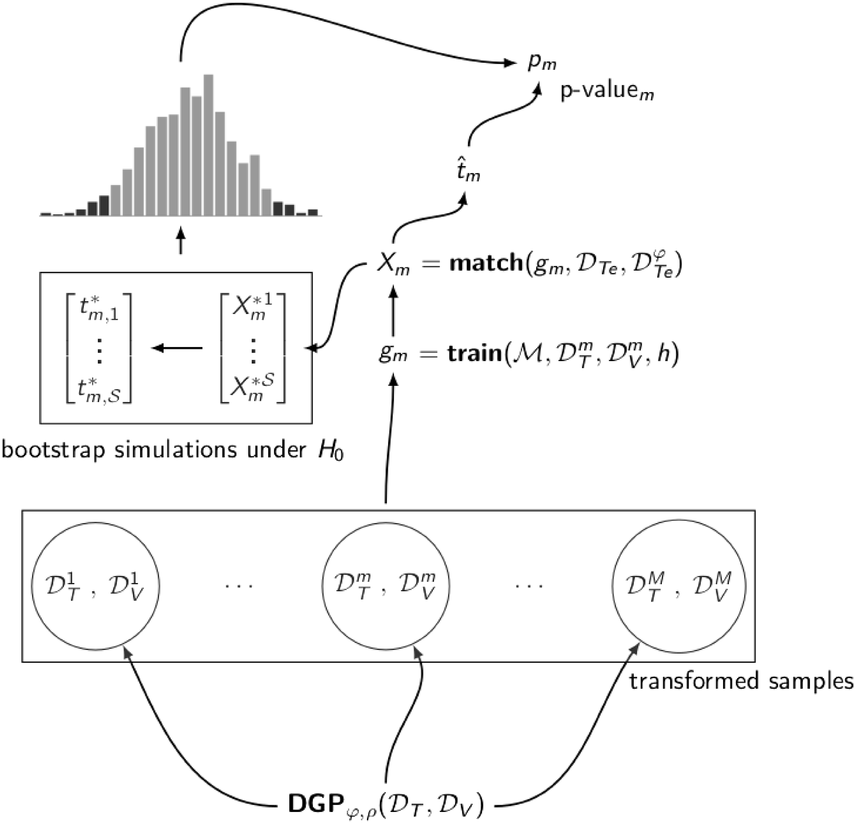
(as illustrated in Figure 1).
$\mathcal{D}_{{Te}}^{\varphi }$
(as illustrated in Figure 1).
The bootstrap version of the paired t-test applied multiple times. For $m = 1, \ldots, M$
,
$m = 1, \ldots, M$
, $g_m$
is a classifier trained on the transformed sample
$g_m$
is a classifier trained on the transformed sample $( \mathcal{D}_{{T}}^{m}, \mathcal{D}_{{V}}^{m})$
. The p-value
$( \mathcal{D}_{{T}}^{m}, \mathcal{D}_{{V}}^{m})$
. The p-value $p_m$
is obtained by comparing the observable test statistic associated with
$p_m$
is obtained by comparing the observable test statistic associated with $g_m$
,
$g_m$
, $\hat{t}_m$
, with the bootstrap distribution of
$\hat{t}_m$
, with the bootstrap distribution of $t$
under the null hypothesis.
$t$
under the null hypothesis.
To assert that a model fails to satisfy the IE property, we check whether at least one classifier based on this model presents a significantly different performance on the two versions of the test set. There is a methodological caveat here. By repeating the same test multiple times the likelihood of incorrectly rejecting the null hypothesis (i.e., the type I error) increases. One widely used correction for this problem is the Bonferroni method (Wasserman Reference Wasserman2010). The method’s application is simple: given a significance level $\alpha$
, after testing
$\alpha$
, after testing $M$
times and acquiring the p-values
$M$
times and acquiring the p-values $p_1, \ldots, p_M$
, we reject the null hypothesis if
$p_1, \ldots, p_M$
, we reject the null hypothesis if $p_m \lt \alpha / M$
for at least one
$p_m \lt \alpha / M$
for at least one $m \in \{1, \ldots, M\}$
.
$m \in \{1, \ldots, M\}$
.
3.4. Invariance under equivalence test
We call Invariance under Equivalence test the whole evaluating procedure of resampling multiple versions of the training data, acquiring different p-values associated with the classifiers’ performance, and, based on these p-values, deciding on the significance of difference between accuracies. The complete description of the test can be found in Algorithm 1.

Many variations of the proposed method are possible. We comment on some options.
Alternative 1. As an alternative to the paired t-test, one can employ the McNemar’s test (McNemar Reference McNemar1947), which is a simplified version of the Cochran’s Q test (Cochram Reference Cochram1950). The McNemar statistic measures the symmetry between the changes in samples. The null hypothesis for this test states that the expected number of observations changed from $A_i=1$
to
$A_i=1$
to $B_i=0$
is the same as the ones changed from
$B_i=0$
is the same as the ones changed from $A_i=0$
to
$A_i=0$
to $B_i=1$
. Thus, the described strategy to resample the matched data (Equation 9) can also be used in this case. The only difference is in the calculation of the p-value, the McNemar’s test is an one-tailed test.
$B_i=1$
. Thus, the described strategy to resample the matched data (Equation 9) can also be used in this case. The only difference is in the calculation of the p-value, the McNemar’s test is an one-tailed test.
Alternative 2. By the stochastic nature of the training algorithm used in the neural network field, there can be performance variation caused only by this algorithm. This is particularly true for deep learning models used in text classification (Dodge et al. Reference Dodge, Ilharco, Schwartz, Farhadi, Hajishirzi and Smith2020). The training variation can be accommodated in our method by estimating multiple classifiers using the same transformed sample and hyperparameter value. After training all those classifiers, one can take the majority vote classifier as the single model $g_m$
.
$g_m$
.
Alternative 3. Since we have defined the hyperparameter selection stage before the resampling process, one single hyperparameter value can influence the training on difference $M$
samples. Another option is to restrict a hyperparameter value to a single sample. Thus, one can first obtain a modified sample and then perform the hyperparameter search.
$M$
samples. Another option is to restrict a hyperparameter value to a single sample. Thus, one can first obtain a modified sample and then perform the hyperparameter search.
All alternatives are valid versions of the method we are proposing and can be implemented elsewhere. It is worth noting that both alternatives 2 and 3 yield a high computational cost, and, in these cases, it is required to train large deep learning models multiple times.
4. Case study: verifying invariance under synonym substitution
As a starting point to understand the effects of equivalent modifications on a NLI task, we have decided to concentrate our focus on transformations based on synonym substitution, that is any text manipulation function that substitutes an occurrence of a word by one of its synonyms.
4.1. Why synonym substitution?
There are many ways to transform a sentence while preserving the original meaning. Although we have listed some examples in Section 2, we will only work with synonym substitution in this article. We explicitly avoid any logical-based transformation. This may sound surprising given the logical inspiration that grounds our project, but such a choice is an effort to create sentences close to everyday life.
It is straightforward to define equivalent transformations based on formal logic. For example, Liu et al. (Reference Liu, Schwartz and Smith2019a) defined a transformation that adds the tautology “and true is true” to the hypothesis (they even define a transformation that appends the same tautology five times to the end of the premise). Salvatore et al. (Reference Salvatore, Finger and Hirata2019) went further and create a set of synthetic data using all sorts of logic-based tools (Boolean coordination, quantifiers, definite description, and counting operators). In both cases, the logical approach generates valuable insights. However, the main weakness of the latter approach is that the sentences produced by logic-based examples do not adequately represent the linguistic variety of everyday speech.
To illustrate this point, take the NLI entailment $P =$
A woman displays a big grin,
$P =$
A woman displays a big grin, $H =$
The woman is happy. We can modify it by creating the new pair (P, H or Q), where
$H =$
The woman is happy. We can modify it by creating the new pair (P, H or Q), where $Q$
is a new sentence. From the rules of formal logic,
$Q$
is a new sentence. From the rules of formal logic, $(P, H)$
implies (P, H or Q). However, when we create sentences using this pattern, they sound highly artificial, for example
$(P, H)$
implies (P, H or Q). However, when we create sentences using this pattern, they sound highly artificial, for example $P^\prime =$
A woman displays a big grin,
$P^\prime =$
A woman displays a big grin, $H^\prime =$
The woman is happy, or a couple is sitting on a bench. Note that, using the same original example
$H^\prime =$
The woman is happy, or a couple is sitting on a bench. Note that, using the same original example $(P, H)$
, we can create a new, and more natural, NLI entailment pair by just substituting smile for grin.
$(P, H)$
, we can create a new, and more natural, NLI entailment pair by just substituting smile for grin.
We mainly use automatic synonym substitution as an attempt to create more spontaneous sentences. As the reader will see in this section, this is far from being a perfect process. The best choice to ensure the production of natural sentences is still a human annotator. Although it is possible to think of a crowdsource setting to ensure the production of high-quality transformations, this comes with some monetary costs. On the other hand, automatic synonym substitution is a cheap and effective solution.
4.2. Defining a transformation function
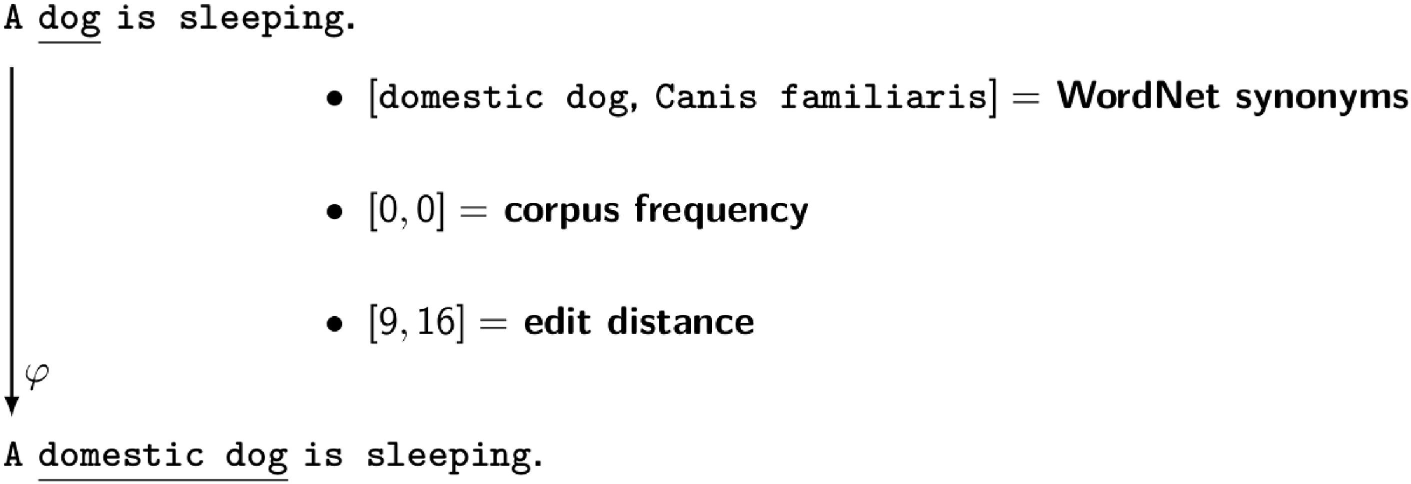
Among the myriad of synonym substitution functions, we have decided to work only with the ones based on the WordNet database (Fellbaum Reference Fellbaum1998). One of the principles behind our analysis is that an equivalent alteration should yield the smallest perturbation possible, hence we have constructed a transformation procedure based on the word frequency of each corpus. We proceed as follows: we utilize the spaCy library (Explosion 2020) to select all nouns in the corpus, then for all nouns we use the WordNet database to list all synonyms and choose the one with the highest frequency. If no synonym appears in the corpus we take the one with the lower edit distance. Figure 2 shows a simple transformation example.
Toy example of sentence transformation (not related to a real dataset). In this case, there are two synonyms associated with the only noun appearing in the source sentence (dog). Since both synonyms have the same frequency in the corpus (zero), the selected synonym is the one with the lower edit distance (domestic dog).
We expand this function to a NLI dataset applying the transformation to both the premise and the hypothesis. In all cases, the target $Y$
remains unchanged.
$Y$
remains unchanged.
4.3. Datasets
We have used the benchmark datasets Stanford Natural Language Inference Corpus (SNLI) (Bowman et al. Reference Bowman, Angeli, Potts and Manning2015) and MultiGenre NLI Corpus (MNLI) (Williams et al. Reference Williams, Nangia and Bowman2018) in our analysis. The SNLI and MNLI datasets are composed of 570K and 433K sentence pairs, respectively. Since the transformation process described above is automatic (allowing us to modify such large datasets), it inevitably causes some odd transformations. Although we have carefully reviewed the transformation routine, we have found some altered sentence pairs that are either ungrammatical or just unusual. For example, take this observation from the SNLI dataset (the relevant words are underlined):
-
1.
$P =$
An old
man
in a
baseball hat
and an old
woman
in a
jean jacket
are standing outside but are covered mostly in shadow.
-
$H =$
An old
woman
has a
light jean jacket
.


Using our procedure, it is transformed on the following pair:
-
1.
${P^{\varphi }} =$
An old
adult male
in a
baseball game hat
and an old
adult female
in a
denim jacket
are standing outside but are covered mostly in shadow.
-
${H^{\varphi }} =$
An old
adult female
has a
visible light denim jacket
.


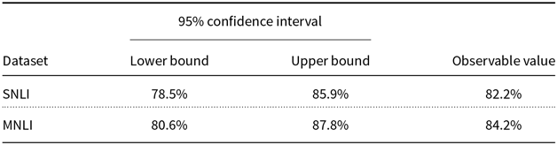
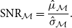
As one can see, the transformation is far from perfect. It does not differentiate the word light from adjective and noun roles. However, unusual expressions as visible light denim jacket form a small part in the altered dataset and the majority of them are sound. To minimize the occurrence of any defective substitutions we have created a block list, that is a list of words that remain unchanged after the transformation. We say that a transformed pair is sound if the modified version is grammatically correct and the original logical relation is maintained. Sometimes due to failures of the POS tagger, the modification function changes adjectives and adverbs (e.g., replacing majestic with olympian). These cases produce modifications beyond the original goal, but we also classify the result transformations as sound if the grammatical structure is maintained. To grasp how much distortion we have added in the process, we estimate the sound percentage for each NLI dataset (Table 1). This quantity is defined as the number of sound transformations in a sample divided by the sample size. In Appendix A, we display some examples of what we call sound and unsound transformations for each dataset.
As can be seen in Table 1, we have added noise in both datasets by applying the transformation function. Hence, in this particular experiment, the reader should know that when we say that two observations (or two datasets) are equivalent, this equivalency is not perfect.
Sound percentages for the transformation function based on the WordNet database. The values were estimated using a random sample of 400 sentence pairs from the training set.
4.4. Methodology
The parameter $\rho$
is a key factor in the IE test because it determines what is a “sufficient amount” of transformation in the training phase. Our initial intuition was that any machine learning model will not satisfy the IE property when we select extreme values of
$\rho$
is a key factor in the IE test because it determines what is a “sufficient amount” of transformation in the training phase. Our initial intuition was that any machine learning model will not satisfy the IE property when we select extreme values of $\rho$
. We believe that the samples generated by those values are biased samples: by choosing low values for
$\rho$
. We believe that the samples generated by those values are biased samples: by choosing low values for $\rho$
there are not enough examples of transformed sentences for the machine learning model in training; similarly, when we use high values for
$\rho$
there are not enough examples of transformed sentences for the machine learning model in training; similarly, when we use high values for $\rho$
there is an over-representation of the modified data in the training phase. Hence, in order to find meaningful values for the transformation probability, we utilize a baseline model to select values for
$\rho$
there is an over-representation of the modified data in the training phase. Hence, in order to find meaningful values for the transformation probability, we utilize a baseline model to select values for $\rho$
where it is harder to refute the null hypothesis. As the baseline, we employ the Gradient Boosting classifier (Hastie, Tibshirani, and Friedman Reference Hastie, Tibshirani and Friedman2001) together with the Bag-of-Words (BoW) representation.
$\rho$
where it is harder to refute the null hypothesis. As the baseline, we employ the Gradient Boosting classifier (Hastie, Tibshirani, and Friedman Reference Hastie, Tibshirani and Friedman2001) together with the Bag-of-Words (BoW) representation.
The main experiment consists in applying the IE test to the recent deep learning models used in NLI: BERT (Devlin et al. Reference Devlin, Chang, Lee and Toutanova2019), XLNet (Yang et al. Reference Yang, Dai, Yang, Carbonell, Salakhutdinov and Le2019), RoBERTa (Liu et al. Reference Liu, Ott, Goyal, Du, Joshi, Chen, Levy, Lewis, Zettlemoyer and Stoyanov2019b), and ALBERT (Lan et al. Reference Lan, Chen, Goodman, Gimpel, Sharma and Soricut2020). In order to repeat the test for different transformation probabilities and altered samples in a feasible time, we utilize only the pre-trained weights associated with the base version of these models. The only exception is for the model RoBERTa. Since this model has a large version fine-tuned on the MNLI dataset, we consider that it is relevant for our investigation to include a version of this model specialized in the NLI task. We use “RoBERTa $_{LARGE}$
” to denote this specific version of the RoBERTa model. For the same reason, we work with a smaller version of each training dataset. Hence, for both SNLI and MNLI datasets we use a random sample of 50K observations for training (this means we are using only
$_{LARGE}$
” to denote this specific version of the RoBERTa model. For the same reason, we work with a smaller version of each training dataset. Hence, for both SNLI and MNLI datasets we use a random sample of 50K observations for training (this means we are using only $8.78\%$
and
$8.78\%$
and $11.54\%$
of the training data of the SNLI and MNLI, respectively). Although this reduction is done to perform the testing, the transformation function is always defined using the whole corpus of each dataset. The MNLI dataset has no labeled test set publicly available. Thus, we use the concatenation of the two development sets (the matched and mismatched data) as the test dataset.
$11.54\%$
of the training data of the SNLI and MNLI, respectively). Although this reduction is done to perform the testing, the transformation function is always defined using the whole corpus of each dataset. The MNLI dataset has no labeled test set publicly available. Thus, we use the concatenation of the two development sets (the matched and mismatched data) as the test dataset.
Because the change in transformation probabilities does not affect the hyperparameter selection stage, we perform a single search for each model and dataset with a budget to train 10 models ( $\mathcal{B}=10$
). In Appendix B, we detail the hyperparameter spaces and the selected hyperparameter values for each model. For each value of
$\mathcal{B}=10$
). In Appendix B, we detail the hyperparameter spaces and the selected hyperparameter values for each model. For each value of $\rho$
, we obtain 5 p-values and perform 1K bootstrap simulations (
$\rho$
, we obtain 5 p-values and perform 1K bootstrap simulations ( $M=5, \mathcal{S}=10^3$
). We set the significance level to
$M=5, \mathcal{S}=10^3$
). We set the significance level to $5\%$
(
$5\%$
( $\alpha = 0.05$
); hence, the adjusted significant level is
$\alpha = 0.05$
); hence, the adjusted significant level is $1\%$
(
$1\%$
( $\alpha / M = 0.01$
). All the deep learning models were implemented using the HuggingFace Transformer Library (Wolf et al. Reference Wolf, Debut, Sanh, Chaumond, Delangue, Moi, Cistac, Rault, Louf, Funtowicz and Brew2019). The code and data used for the experiments can be found in (Salvatore Reference Salvatore2020).
$\alpha / M = 0.01$
). All the deep learning models were implemented using the HuggingFace Transformer Library (Wolf et al. Reference Wolf, Debut, Sanh, Chaumond, Delangue, Moi, Cistac, Rault, Louf, Funtowicz and Brew2019). The code and data used for the experiments can be found in (Salvatore Reference Salvatore2020).
5. Results
In this section, we present the results and findings of the experiments with the synonym substitution function on SNLI and MNLI datasets. First, we describe how changing the transformation probability $\rho$
affects the test for the baseline model. Second, we apply the IE test for the deep learning models using the evenly distributed values for
$\rho$
affects the test for the baseline model. Second, we apply the IE test for the deep learning models using the evenly distributed values for $\rho$
. We comment on the test results and observe how to utilize the experiment outcome to measure the robustness of the NLI models.
$\rho$
. We comment on the test results and observe how to utilize the experiment outcome to measure the robustness of the NLI models.
5.1. Baseline exploration
To mitigate the cost of training deep learning models, we have used the baseline (the Gradient Boosting classifier with a BoW representation) to find the intervals between 0 and 1 where rejecting the null hypothesis is not a trivial exercise. Figure 3 shows the test results associated with the baseline for each dataset using 101 different choices of $\rho$
(values selected from the set
$\rho$
(values selected from the set $\{0, 0.01, 0.02, \ldots, 0.98, 0.99, 1\}$
).
$\{0, 0.01, 0.02, \ldots, 0.98, 0.99, 1\}$
).
Baseline results. In the $x$
-axis, we have different choices of transformation probabilities used in training. The
$x$
-axis, we have different choices of transformation probabilities used in training. The $y$
-axis displays the minimum value for the p-values acquired in five paired t-tests. We reject the null hypothesis if the minimum p-value is smaller than
$y$
-axis displays the minimum value for the p-values acquired in five paired t-tests. We reject the null hypothesis if the minimum p-value is smaller than $1\%$
.
$1\%$
.
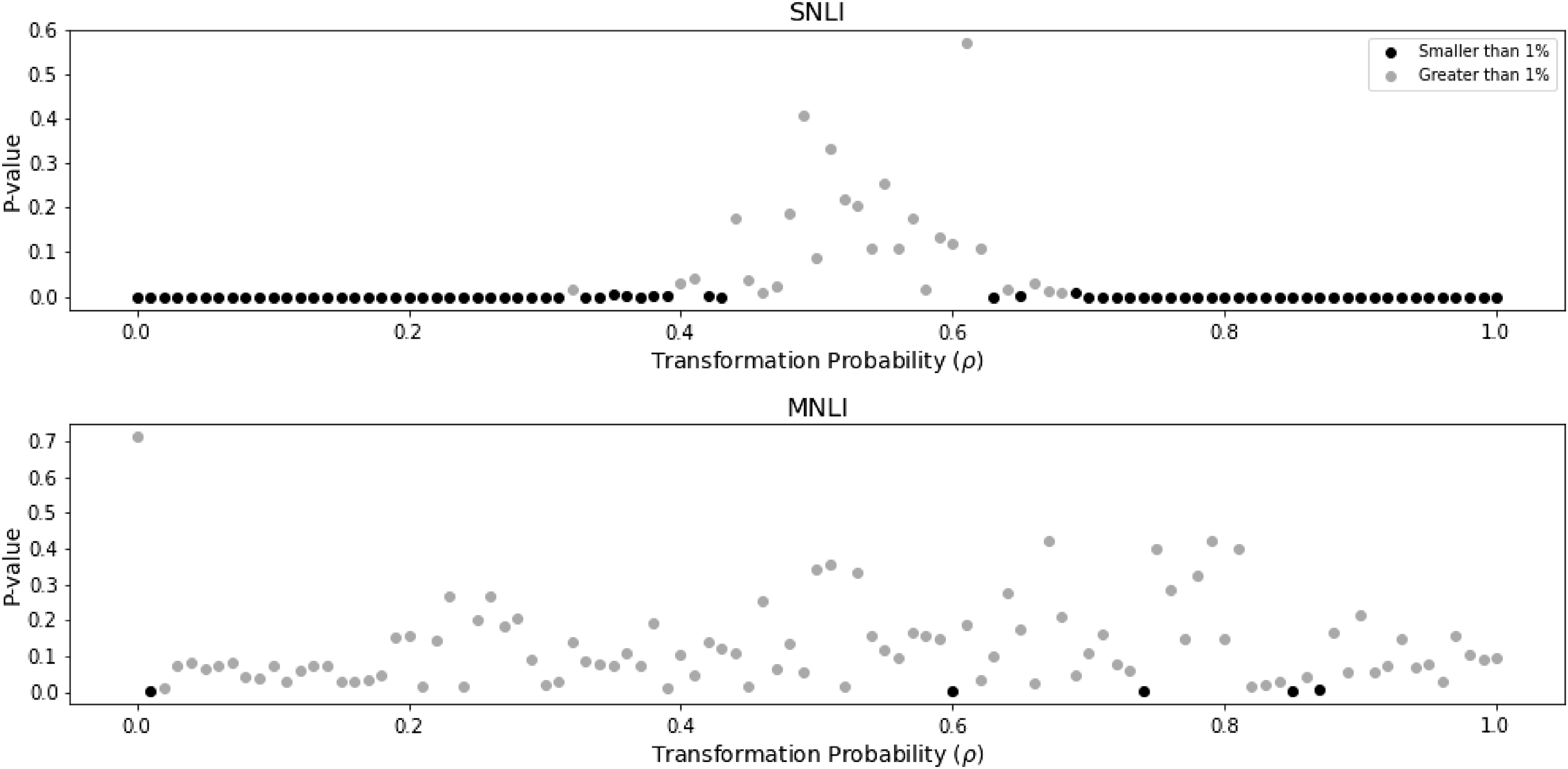
The results for the SNLI data are in agreement with our initial intuition: on the one hand, choosing extremes values for $\rho$
(values from the intervals
$\rho$
(values from the intervals $[0, 0.2]$
and
$[0, 0.2]$
and $[0.8, 1.0]$
) yields p-values concentrated closer to zero, and so rejecting the null hypothesis at
$[0.8, 1.0]$
) yields p-values concentrated closer to zero, and so rejecting the null hypothesis at $5\%$
significance level. On the other hand, when choosing a transformation probability in the interval
$5\%$
significance level. On the other hand, when choosing a transformation probability in the interval $[0.4, 0.6]$
, we are adding enough transformed examples for training, and so we were not able the reject the null hypothesis. The same phenomenon cannot be replicated in the MNLI dataset. It seems that for this dataset the introduction of transformed examples does not change the baseline performance—independently of the choice of
$[0.4, 0.6]$
, we are adding enough transformed examples for training, and so we were not able the reject the null hypothesis. The same phenomenon cannot be replicated in the MNLI dataset. It seems that for this dataset the introduction of transformed examples does not change the baseline performance—independently of the choice of $\rho$
. Although we are able to obtain p-values smaller than
$\rho$
. Although we are able to obtain p-values smaller than $1\%$
in five scenarios (namely for
$1\%$
in five scenarios (namely for $\rho \in \{ 0.01, 0.6, 0.74, 0.85, 0.87\}$
), the SNLI pattern does not repeat in the MNLI dataset.
$\rho \in \{ 0.01, 0.6, 0.74, 0.85, 0.87\}$
), the SNLI pattern does not repeat in the MNLI dataset.
By taking a closer look at the sentences from both datasets, we offer the following explanation. SNLI is composed of more repetitive and simple sentence types. For example, from all modifications we can perform on this dataset, $12\%$
are modifications that substitute man with adult male. This phenomenon corresponds to the excessive number of sentences of the type
$12\%$
are modifications that substitute man with adult male. This phenomenon corresponds to the excessive number of sentences of the type $P =$
A man VERB
$P =$
A man VERB $\ldots$
. On the other hand, when we look at MNLI sentences, we do not see a clear predominance of a sentence type. A more detailed analysis is presented in Appendix C.
$\ldots$
. On the other hand, when we look at MNLI sentences, we do not see a clear predominance of a sentence type. A more detailed analysis is presented in Appendix C.
The baseline exploration gives us the following intuition: the synonym substitution transformation changes the inference of a classifier on the SNLI dataset for extreme $\rho$
values. But, we do not expect the same transformation to change a classifier’s outputs for the MNLI dataset.
$\rho$
values. But, we do not expect the same transformation to change a classifier’s outputs for the MNLI dataset.
5.2. Testing deep learning models
The baseline has helped us to identify the interval of transformation probabilities where the performances on the two versions of the test set might be similar: the interval $[0.4, 0.6]$
. Based on that information, we have chosen three values from this interval for the new tests, namely,
$[0.4, 0.6]$
. Based on that information, we have chosen three values from this interval for the new tests, namely, $0.4, 0.5$
, and
$0.4, 0.5$
, and $0.6$
. To obtain a broader representation, we have also selected two values for
$0.6$
. To obtain a broader representation, we have also selected two values for $\rho$
in both extremes. Hence, we have tested the deep learning models using seven values for
$\rho$
in both extremes. Hence, we have tested the deep learning models using seven values for $\rho$
:
$\rho$
: $0, 0.2, 0.4, 0.5, 0.6, 0.8, 1$
.
$0, 0.2, 0.4, 0.5, 0.6, 0.8, 1$
.
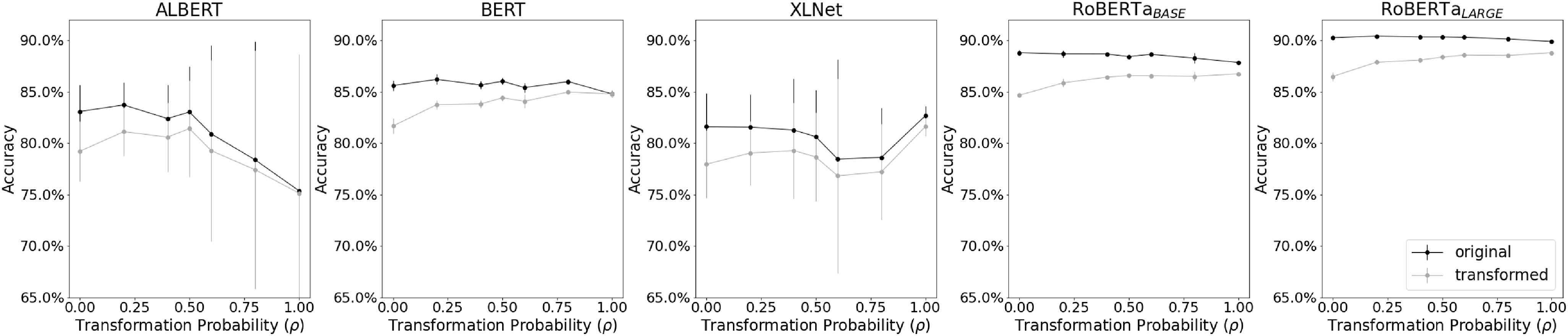
According to the test accuracies (Figures 4 and 5), we observe that ROBERTA $_{LARGE}$
is the best model. This is an expected result. ROBERTA
$_{LARGE}$
is the best model. This is an expected result. ROBERTA $_{LARGE}$
is the larger version of the ROBERTA model with an architecture composed of more layers and attention heads. Not only does ROBERTA
$_{LARGE}$
is the larger version of the ROBERTA model with an architecture composed of more layers and attention heads. Not only does ROBERTA $_{LARGE}$
outperform ROBERTA
$_{LARGE}$
outperform ROBERTA $_{BASE}$
in different language understanding tasks (Liu et al. Reference Liu, Ott, Goyal, Du, Joshi, Chen, Levy, Lewis, Zettlemoyer and Stoyanov2019b), but also the specific version of the ROBERTA
$_{BASE}$
in different language understanding tasks (Liu et al. Reference Liu, Ott, Goyal, Du, Joshi, Chen, Levy, Lewis, Zettlemoyer and Stoyanov2019b), but also the specific version of the ROBERTA $_{LARGE}$
model used in our experiments was fine-tuned on the MNLI dataset.
$_{LARGE}$
model used in our experiments was fine-tuned on the MNLI dataset.
SNLI results. In the $x$
-axis, we have different choices of transformation probabilities in training. The
$x$
-axis, we have different choices of transformation probabilities in training. The $y$
-axis displays the accuracy. Each point represents the average accuracy in five runs. The vertical lines display the associated standard deviation. The black and gray lines represent the values for the original and transformed test sets, respectively.
$y$
-axis displays the accuracy. Each point represents the average accuracy in five runs. The vertical lines display the associated standard deviation. The black and gray lines represent the values for the original and transformed test sets, respectively.
MNLI results. In the $x$
-axis, we have different choices of transformation probabilities in training. The
$x$
-axis, we have different choices of transformation probabilities in training. The $y$
-axis displays the accuracy. Each point represents the average accuracy in five runs. The vertical lines display the associated standard deviation. The black and gray lines represent the values for the original and transformed test sets, respectively.
$y$
-axis displays the accuracy. Each point represents the average accuracy in five runs. The vertical lines display the associated standard deviation. The black and gray lines represent the values for the original and transformed test sets, respectively.
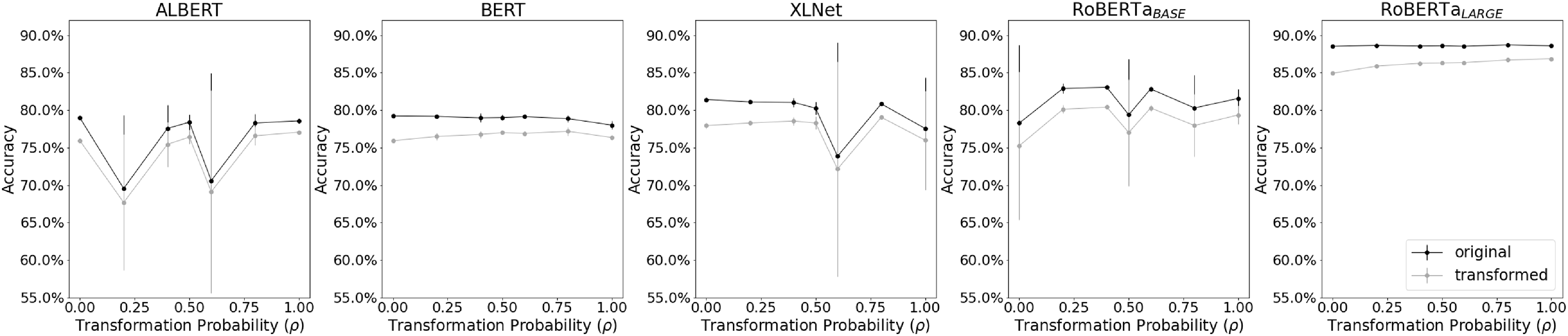
Each model is affected differently by the change in $\rho$
. On the SNLI dataset (Figure 4), all models, except for ALBERT, continue to show a high accuracy even when we use a fully transformed training dataset. We have a similar picture on the MNLI dataset (Figure 5). However, in the latter case, we notice a higher dispersion in the accuracies for the models ALBERT, XLNet, and ROBERTA
$\rho$
. On the SNLI dataset (Figure 4), all models, except for ALBERT, continue to show a high accuracy even when we use a fully transformed training dataset. We have a similar picture on the MNLI dataset (Figure 5). However, in the latter case, we notice a higher dispersion in the accuracies for the models ALBERT, XLNet, and ROBERTA $_{BASE}$
.
$_{BASE}$
.
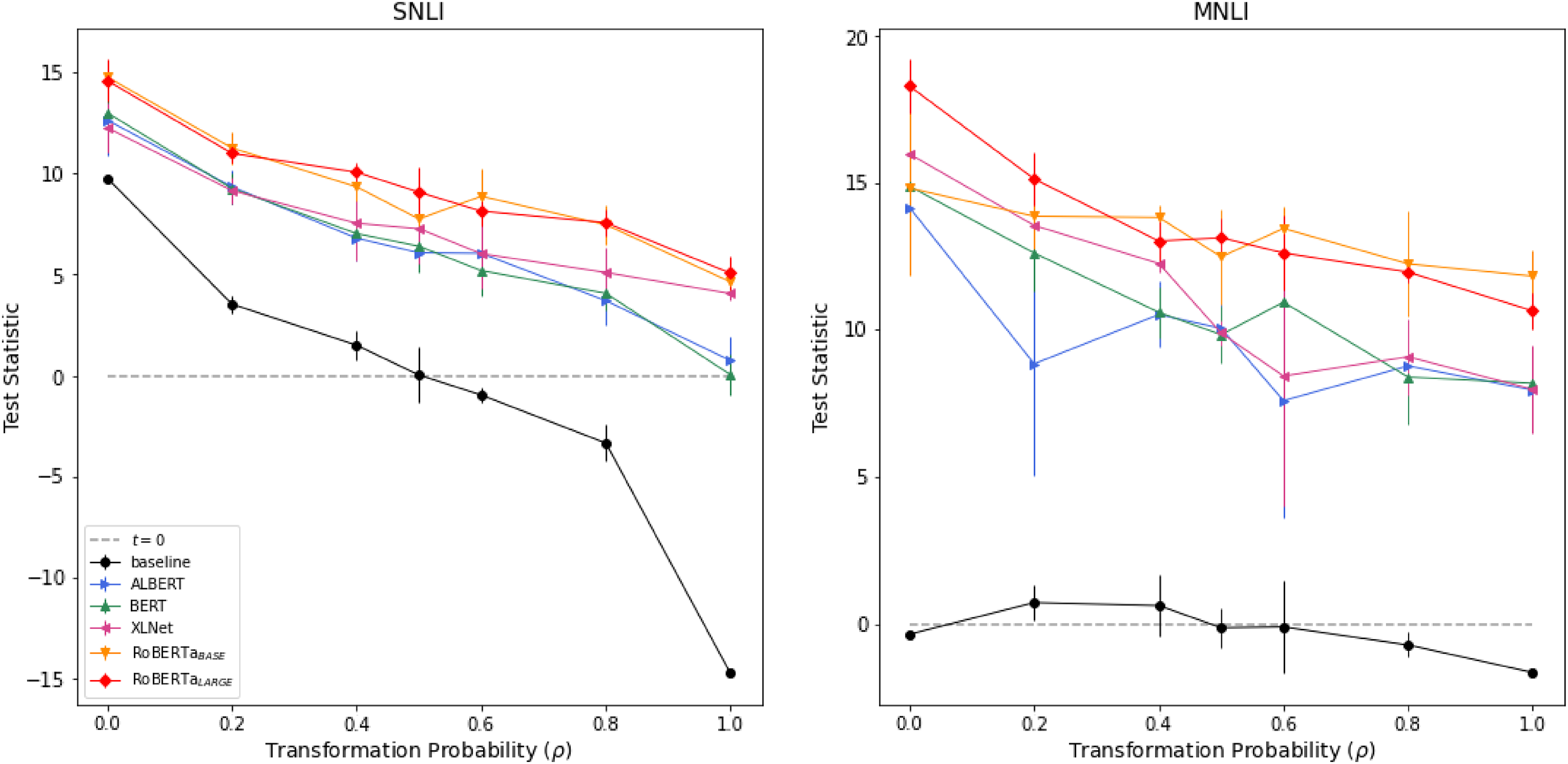
In the majority of cases, we also observe that the performance on the original test set is superior compared to the transformed version as expected. As seen in Figures 4 and 5, in almost all choices of $\rho$
and for all deep learning models, the black line (the accuracy on the original test set) dominates the gray line (the accuracy on the transformed version of the test set). This difference becomes more evident for the test statistic (Figure 6). For almost every choice of
$\rho$
and for all deep learning models, the black line (the accuracy on the original test set) dominates the gray line (the accuracy on the transformed version of the test set). This difference becomes more evident for the test statistic (Figure 6). For almost every choice of $\rho$
, all deep learning models have generated test statistics with extremely positive values. When we compare these statistics with the empirical distribution generated under the null hypothesis we obtain p-values smaller than
$\rho$
, all deep learning models have generated test statistics with extremely positive values. When we compare these statistics with the empirical distribution generated under the null hypothesis we obtain p-values smaller than $10^{-4}$
for the majority of cases. The exceptions are related to the models ALBERT and BERT on the SNLI dataset using
$10^{-4}$
for the majority of cases. The exceptions are related to the models ALBERT and BERT on the SNLI dataset using $\rho =1$
. In these cases, the minimal p-values are
$\rho =1$
. In these cases, the minimal p-values are $0.008$
and
$0.008$
and $0.156$
, respectively. Hence, for all IE tests associated with the deep learning models, we reject the null hypothesis in
$0.156$
, respectively. Hence, for all IE tests associated with the deep learning models, we reject the null hypothesis in $69$
tests out of
$69$
tests out of $70$
.
$70$
.
Test statistics from the IE test for all models. In the $x$
-axis, we have different choices of transformation probabilities used in training. The
$x$
-axis, we have different choices of transformation probabilities used in training. The $y$
-axis displays the values for the test statistic. Each point represents the average test statistics in five paired t-tests. The vertical lines display the associated standard deviation. And the baseline is a BoW model.
$y$
-axis displays the values for the test statistic. Each point represents the average test statistics in five paired t-tests. The vertical lines display the associated standard deviation. And the baseline is a BoW model.
The empirical evidence shows that the deep learning models are not invariant under equivalence. To better assess the qualitative aspect of this result, we have added in Appendix C an estimation of the sound percentage of the test sets and comment on some particular results. Most sentences in the tests set of SNLI and MNLI are sound. Hence, it seems that the difference in performance is not just a side effect of the transformation function. This indicates that although these models present an impressive inference capability, they still lack the skill of producing the same deduction based on different sentences with the same meaning. After rejecting the null hypothesis when using different transformation probabilities, we are convinced that this is not a simple data acquisition problem. Since we are seeing the same pattern for almost all models in both datasets, it seems that the absence of the invariance under equivalence propriety is a feature in the Transformer-based models.
5.3. Experimental finding: model robustness
We now concentrate on a notion of prediction robustness under a transformation function. One possible interpretation of the transformation function is that this alteration can be seen as a noise that is imposed to the training data. Although this type of noise is imperceptible for humans, it can lead the machine learning model to make wrong predictions. By this interpretation, the transformation function is an “adversary,” an “attack,” or a “challenge” to the model (Liu et al. Reference Liu, Schwartz and Smith2019a). Along these lines, a robust model is one that consistently produces high test accuracy even when we add different proportions of noised observations in training; in other words, a robust model should combine higher prediction power and low accuracy variation. Given a model $\mathcal{M}$
and a dataset, we train the model using the
$\mathcal{M}$
and a dataset, we train the model using the $(\varphi, \rho )$
data generation process for different values of
$(\varphi, \rho )$
data generation process for different values of $\rho$
(as before
$\rho$
(as before $\rho \in [0,1]$
) and obtain a sample of test accuracies (accuracies associated with the original test set). In this article, we use the signal-to-noise ratio (SNR) as a measure of robustness. Let
$\rho \in [0,1]$
) and obtain a sample of test accuracies (accuracies associated with the original test set). In this article, we use the signal-to-noise ratio (SNR) as a measure of robustness. Let $\hat{\mu }_{\mathcal{M}}$
and
$\hat{\mu }_{\mathcal{M}}$
and $\hat{\sigma }_{\mathcal{M}}$
be the sample mean and standard deviation of the accuracies, respectively, we define:
$\hat{\sigma }_{\mathcal{M}}$
be the sample mean and standard deviation of the accuracies, respectively, we define:
 \begin{equation} \text{SNR}_{\mathcal{M}} = \frac{\hat{\mu }_{\mathcal{M}}}{\hat{\sigma }_{\mathcal{M}}}. \end{equation}
This statistical measure has an intuitive interpretation: the numerator represents the model’s overall performance when noise is added, and the denominator indicates how much the model’s predictive power changes when different levels of noise are present. Hence, the larger, the better. Since this score can be given for each model and dataset, we rank the models by their robustness under a transformation function by averaging the model’s SNR on different datasets (Table 2).
Ranked models according to the SNR metric. In this case, the noise is the synonym substitution transformation.

From the perspective of robustness—based only on the SNR metric—the networks XLNet and ALBERT are worse than the baseline. Although both deep learning models present, on average, a higher accuracy compared to the baseline; they are not able to maintain high accuracy when different quantities of altered sentences are included in the training data. In contrast, the baseline produces a low yet consistent test accuracy (Figure 7). Among all models, BERT and ROBERTA appear to be the most robust ones. As seen in Table 2, BERT shows consistent performance in both datasets, and ROBERTA $_{BASE}$
shows an almost unchanged behavior on the SNLI dataset. Clearly, ROBERTA
$_{BASE}$
shows an almost unchanged behavior on the SNLI dataset. Clearly, ROBERTA $_{LARGE}$
stands out when compared to the rest. This model was not only able to obtain a higher accuracy on both datasets but also it had maintained a high performance regardless of the choice of
$_{LARGE}$
stands out when compared to the rest. This model was not only able to obtain a higher accuracy on both datasets but also it had maintained a high performance regardless of the choice of $\rho$
.
$\rho$
.
Models’ accuracy on the original test set. In the $x$
-axis, we have different choices of transformation probabilities used in training. The
$x$
-axis, we have different choices of transformation probabilities used in training. The $y$
-axis displays the accuracy. Each point represents the average accuracy in five runs. The vertical lines display the associated standard deviation. And the baseline is a BoW model.
$y$
-axis displays the accuracy. Each point represents the average accuracy in five runs. The vertical lines display the associated standard deviation. And the baseline is a BoW model.

5.4. Discussion and limitations
The result of the IE tests applied to the deep learning models shows that these models can have different inferences for sentences with the same meaning. What is surprising about the deep learning models is that they perform very differently in the test sets $\mathcal{D}_{{Te}}$
and
$\mathcal{D}_{{Te}}$
and $\mathcal{D}_{{Te}}^{\varphi }$
even when sufficient amount of transformed observations are added in training. We offer a possible explanation for this phenomenon. All transformed-based models are trained in two stages: they are pre-trained using unlabeled text and fine-tuned for the NLI task. The
$\mathcal{D}_{{Te}}^{\varphi }$
even when sufficient amount of transformed observations are added in training. We offer a possible explanation for this phenomenon. All transformed-based models are trained in two stages: they are pre-trained using unlabeled text and fine-tuned for the NLI task. The $(\varphi, \rho )$
data generation process only affects the fine-tuning phase. Hence, we believe that it is possible to reduce the accuracy difference between the two versions of the test data by allowing the addition of transformed sentences in the pre-training stage. However, since pre-training these large models is a computationally expensive endeavor, the results presented here are relevant. It seems that we cannot correct how these models perform inference by just adding examples in the fine-tuning phase.
$(\varphi, \rho )$
data generation process only affects the fine-tuning phase. Hence, we believe that it is possible to reduce the accuracy difference between the two versions of the test data by allowing the addition of transformed sentences in the pre-training stage. However, since pre-training these large models is a computationally expensive endeavor, the results presented here are relevant. It seems that we cannot correct how these models perform inference by just adding examples in the fine-tuning phase.
There is a limitation in the present analysis. As stated in the methodological considerations (Section 4.4), we have used a small random sample of the training data (small compared to the original size of the SNLI and MNLI dataset). Hence, one can argue that the results associated with the deep learning models are restricted to small NLI datasets. Further research is needed to verify this claim. We can take bigger samples (samples with more than 50K observations) and apply the IE test to verify if there is a minimum training size needed to correct the biases of the deep learning models in the fine-tuning phase. Even if such minimum size exists, our results expose some limitations of the current NLI models. The results presented here may serve as motivation for a broader exploration on those limits.
Our battery of experiments does not include the recently released dynamic datasets (Nie et al. Reference Nie, Williams, Dinan, Bansal, Weston and Kiela2020; Kiela et al. Reference Kiela, Bartolo, Nie, Kaushik, Geiger, Wu, Vidgen, Prasad, Singh, Ringshia, Ma, Thrush, Riedel, Waseem, Stenetorp, Jia, Bansal, Potts and Williams2021; Ma et al. Reference Ma, Ethayarajh, Thrush, Jain, Wu, Jia, Potts, Williams and Kiela2021). Hence, a natural extension of our work will be the inclusion of these new data sources. It should be noted that the dynamic datasets are still an open challenge for the transformer-based models, and both SNLI and MNLI are solved inference tasks. Our results show that even in tasks where machine learning models surpass human performance, it is possible to find logical blind spots.
6. Related work
There is an established line of work in NLI that uses adversarial techniques. They all show the limitations of the machine learning models when trained in the classical inference datasets.
Glockner et al. (Reference Glockner, Shwartz and Goldberg2018) developed a new test set based on different types of lexical knowledge (e.g., hypernymy and hyponymy relations). They showed that machine learning models trained on the datasets SNLI and MNLI perform substantially worse on their new lexical test set.
Nie et al. (Reference Nie, Wang and Bansal2018) created a new test set where the logical relations do not depend on lexical information alone (e.g., it is possible to obtain a new contradiction observation $(P, P^{\prime })$
from the pair
$(P, P^{\prime })$
from the pair $(P,H)$
, where
$(P,H)$
, where $P^\prime$
is the result of swapping the subject and object in
$P^\prime$
is the result of swapping the subject and object in $P$
). They showed that models trained on SNLI perform poorly on their new adversarial test sets.
$P$
). They showed that models trained on SNLI perform poorly on their new adversarial test sets.
Dasgupta et al. (Reference Dasgupta, Guo, Stuhlmüller, Gershman and Goodman2018) constructed a test set based on word composition (e.g., some entailment examples have the form: $P = X$
is more cheerful than
$P = X$
is more cheerful than $Y$
, and
$Y$
, and $H = Y$
is less cheerful than
$H = Y$
is less cheerful than $X$
). They have observed that different models trained on the SNLI dataset perform badly on their adversarial test set; however, they also noted that performance can be corrected when the models are trained with observations similar as the ones from the new test set.
$X$
). They have observed that different models trained on the SNLI dataset perform badly on their adversarial test set; however, they also noted that performance can be corrected when the models are trained with observations similar as the ones from the new test set.
Naik et al. (Reference Naik, Ravichander, Sadeh, Rose and Neubig2018) offered three new adversarial test sets (they have called them “stress tests”) based on different linguistic phenomena (e.g., antonymy relation, sentences containing numerals, etc.). After training different models on the MNLI dataset, they have observed that the models show a significant performance drop on their new test sets.
McCoy et al. (Reference McCoy, Pavlick and Linzen2019) observed three “syntactical heuristics” presented on the benchmark datasets: lexical overlap heuristic (the logical relation can be guessed solely based on word overlap); subsequent heuristic (the logical relation can be guessed solely based on the fact that $H$
is a subsequence of
$H$
is a subsequence of $P$
); and constituent heuristic (the logical relation can be guessed from the fact that
$P$
); and constituent heuristic (the logical relation can be guessed from the fact that $H$
is a constituent of
$H$
is a constituent of $P$
). In order to understand how much a machine learning model rely on such heuristics, McCoy et al. (Reference McCoy, Pavlick and Linzen2019) constructed an adversarial test set where those heuristic fail. They showed that different models trained on the MNLI dataset perform very poorly on their adversarial test set. Similar to Dasgupta et al. (Reference Dasgupta, Guo, Stuhlmüller, Gershman and Goodman2018), they also noted that it is possible to obtain good performances on the new test set when similar observations are introduced in the training stage.
$P$
). In order to understand how much a machine learning model rely on such heuristics, McCoy et al. (Reference McCoy, Pavlick and Linzen2019) constructed an adversarial test set where those heuristic fail. They showed that different models trained on the MNLI dataset perform very poorly on their adversarial test set. Similar to Dasgupta et al. (Reference Dasgupta, Guo, Stuhlmüller, Gershman and Goodman2018), they also noted that it is possible to obtain good performances on the new test set when similar observations are introduced in the training stage.
Yanaka et al. (Reference Yanaka, Mineshima, Bekki, Inui, Sekine, Abzianidze and Bos2019) constructed a new test set based on monotonicity inference (this term includes different linguistic phenomena that can cause entailment, e.g., the removal of modifiers—I bought a movie ticket entails I bought a ticket). After training different models on the SNLI and MNLI datasets, they have observed that the performance of the machine learning models on their adversarial test set was unsatisfactory. They have also noted that the performance of the models can be improved when monotonicity inference examples are added when training those models.
Similar to the present article, Liu et al. (Reference Liu, Schwartz and Smith2019a) proposed an analysis of the limitation of datasets and models from the NLI literature by defining a collection of transformation functions (“challenges to benchmarks”) and a training procedure that includes transformed observations (“inoculation by fine-tuning”). Note that, the IE test can be seen as a generalization of this type of analysis. In the process of inoculation, the authors fix a “small number” of transformed examples for training and compare model performance on two test sets ignoring any statistical significance test. By contrast, our method allows any portion of the training data to be altered.
Our analysis was directly influenced by Geiger et al. (Reference Geiger, Cases, Karttunen and Potts2019). The authors of that work have used the notion of fairness to argue that an evaluation method is not fair if the model was not trained on a sample that does not support the required generalization. The IE test is an alternative tool to approach the fairness problem. In our experiment, we performed an exploratory analysis to select some particular values for $\rho$
that could generate non-biased samples (our version of “fair datasets”). Through experimentation, we selected the values
$\rho$
that could generate non-biased samples (our version of “fair datasets”). Through experimentation, we selected the values $0.4$
,
$0.4$
, $0.5,$
and
$0.5,$
and $0.6$
. But other researchers may take an alternative route. They can pre-define some values for
$0.6$
. But other researchers may take an alternative route. They can pre-define some values for $\rho$
that they judge “fair” (e.g.,
$\rho$
that they judge “fair” (e.g., $0.25, 0.5, 0.75$
) and run all the comparisons.
$0.25, 0.5, 0.75$
) and run all the comparisons.
Although it is a work in machine translation literature, Hupkes et al. (Reference Hupkes, Dankers, Mul and Bruni2020) defined a consistent score to measure how consistent models’ predictions are—correct or incorrect—when a word is replaced with a synonym. Similar to our results on robustness, they observed that, compared to other models, the Transformer-based models show a high consistency score.
7. Conclusions
In this article, we have developed the IE test, a method to evaluate whether an NLI model can make the same type of inference for equivalent text inputs. By using an equivalent transformation function based on synonym substitution we have tested the state-of-the-art models and observed that these models show two different inferences for two sentences with the same meaning. We have also ranked these models by their performance robustness when transformed data is introduced.
The results presented here show only a partial picture of the limitations of the current NLI models. The present analysis can be improved using the IE test in a broader study to investigate whether the IE property is violated for other models and datasets. There are already new powerful models to be analyzed, for example DeBERTa, DeBERTaV3, and T5 (He et al. Reference He, Liu, Gao and Chen2020; He, Gao, and Chen Reference He, Gao and Chen2021; Raffel et al. Reference Raffel, Shazeer, Roberts, Lee, Narang, Matena, Zhou, Li and Liu2020). And as mentioned before, the recent trend of dynamic models will keep providing good data sources for the NLI community (Nie et al. Reference Nie, Williams, Dinan, Bansal, Weston and Kiela2020; Kiela et al. Reference Kiela, Bartolo, Nie, Kaushik, Geiger, Wu, Vidgen, Prasad, Singh, Ringshia, Ma, Thrush, Riedel, Waseem, Stenetorp, Jia, Bansal, Potts and Williams2021; Ma et al. Reference Ma, Ethayarajh, Thrush, Jain, Wu, Jia, Potts, Williams and Kiela2021).
Moreover, we have used only English corpora, but our analysis can be extended to other languages, with a caveat. We assume the language being studied has the same tools as those used here. For example, it is possible to perform the same synonym substitution analysis for Portuguese because there are NLI datasets in Portuguese (Real et al. Reference Real, Rodrigues, Vieira, Albiero, Thalenberg, Guide, Silva, Lima, Câmara, Stanojević, Souza and De Paiva2018; Fonseca et al. Reference Fonseca, Borges dos Santos, Criscuolo and Aluísio2016), and there is a counterpart of the WordNet in Portuguese (De Paiva et al. Reference De Paiva, Real, Gonçalo Oliveira, Rademaker, Freitas and Simões2016). Crowdsource labor is needed for any language that does not already have these tools.
From the theoretical side, there is still space for improvement. The IE test is based on resampling an altered version of the dataset multiple times. When combining this strategy with models with hundreds of millions of parameters, we can quickly encounter hardware and time limitations. Thus, a natural continuation of this research path is to combine the resampling method with the reduction techniques that can increase training and inference speed.
The IE test is a tool to comprehend the deficiency of machine learning models. Since equivalence in natural language is based on the general phenomenon of meaning identity, extending this test for any text classification task is reasonable. This extension should be carefully established because the definition of an adequate transformation function is task-dependent. After selecting a transformation, the IE test can be used to check for any biases in the transformer-based models’ pre-training. We hope that our evaluation procedure encourages and facilitates such limitation analysis.
Acknowledgements
This study was financed in part by the Coordenação de Aperfeiçoamento de Pessoal de Nível Superior – Brasil (CAPES) [Finance Code 001]; the São Paulo Research Foundation (FAPESP) [grants #2015/21880-4, #2014/12236-1, #2015/22308-2, #2015/24485-9, #2018/21934-5]; and the National Council for Scientific and Technological Development (CNPq) [grant PQ 303609/2018-4]. This work was carried out at the Center for Artificial Intelligence (C4AI-USP), with support from the São Paulo Research Foundation (FAPESP) [grant #2019/07665-4] and by the IBM Corporation.
Appendix A: Synonym substitution examples
The distinction between sound and unsound transformations is based on subjective judgments. What has guided us to determine an alteration as sound is how the transformation affects the associated label. Hence, we have allowed modifications that produce minor grammatical errors (e.g., “a adult male”). Tables 3–6 show some examples of sound and unsound transformations.
Sound transformations for SNLI.

Unsound transformations for SNLI.
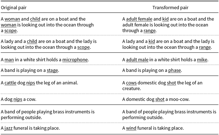
Sound transformations for MNLI.
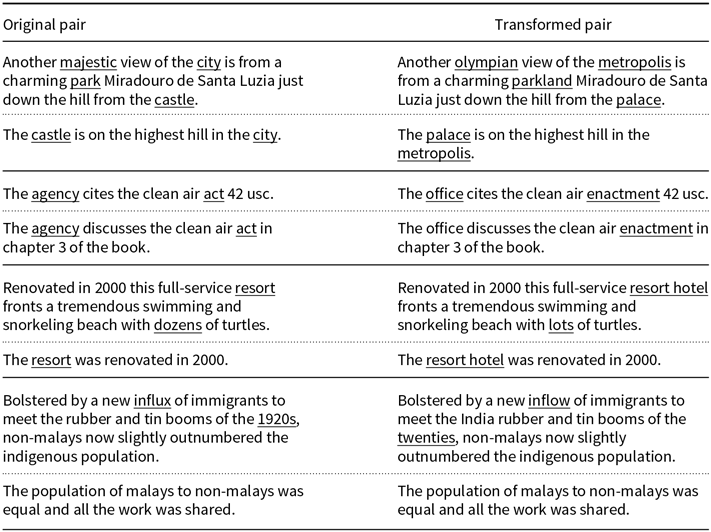
Unsound transformations for MNLI.

Appendix B: Hyperparameter search
We present all the hyperparameters used in training, the associated search space, and the selected value for each dataset in Tables 7–12. The hyperparameter values were selected using the random search algorithm.
Gradient boosting
Best hyperparameter assignments for the Gradient Boosting classifier.
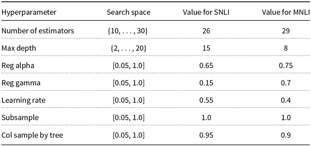
ALBERT
Best hyperparameter assignments for ALBERT.
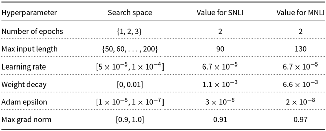
BERT
Best hyperparameter assignments for BERT.
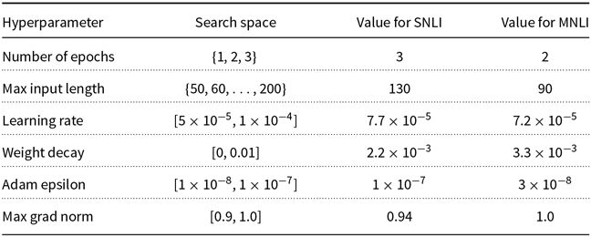
XLNet
Best hyperparameter assignments for XLNet.

RoBERTa
$_{BASE}$

Best hyperparameter assignments for RoBERTa $_{BASE}$
.
$_{BASE}$
.
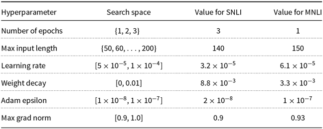
RoBERTa
$_{LARGE}$

Best hyperparameter assignments for RoBERTa $_{LARGE}$
.
$_{LARGE}$
.

Appendix C: Qualitative analysis
To give the reader a holistic view of the modifications, we describe in more detail the different effects caused by the synonym substitution function.
Most frequent tranformations
The SNLI training data contains $550$
K sentence pairs. Among these observations,
$550$
K sentence pairs. Among these observations, $93\%$
can be transformed using our synonym substitution function. On average,
$93\%$
can be transformed using our synonym substitution function. On average, $3.25$
words were transformed per sentence pair. Similarly, the MNLI training dataset comprises
$3.25$
words were transformed per sentence pair. Similarly, the MNLI training dataset comprises $392$
K sentence pairs. When we apply the synonym substitution function to all the dataset, we modify
$392$
K sentence pairs. When we apply the synonym substitution function to all the dataset, we modify $91\%$
of the data. On average,
$91\%$
of the data. On average, $4.23$
words were transformed per sentence pair in this dataset.
$4.23$
words were transformed per sentence pair in this dataset.
Domain difference affects the behavior of the transformation function. Since the SNLI dataset contains more generic phrases, we observe that an expressive number of transformations in this dataset are based on modifying the words men, woman, boy, and person. As displayed in Figure 8, the substitution of man by adult male is responsible for more than $12\%$
of all sentence modifications. On the other hand, since the MNLI data are composed of more domain-specific terms, we do not see a clear pattern in the transformation. As can be seen in Figure 8, the modification on the MNLI test set is not strongly influenced by a few words.
$12\%$
of all sentence modifications. On the other hand, since the MNLI data are composed of more domain-specific terms, we do not see a clear pattern in the transformation. As can be seen in Figure 8, the modification on the MNLI test set is not strongly influenced by a few words.
Plot with the twenty most frequent transformations of each dataset. The $x$
-axis displays the word substitution frequency. The
$x$
-axis displays the word substitution frequency. The $y$
-axis displays the content of each substitution.
$y$
-axis displays the content of each substitution.
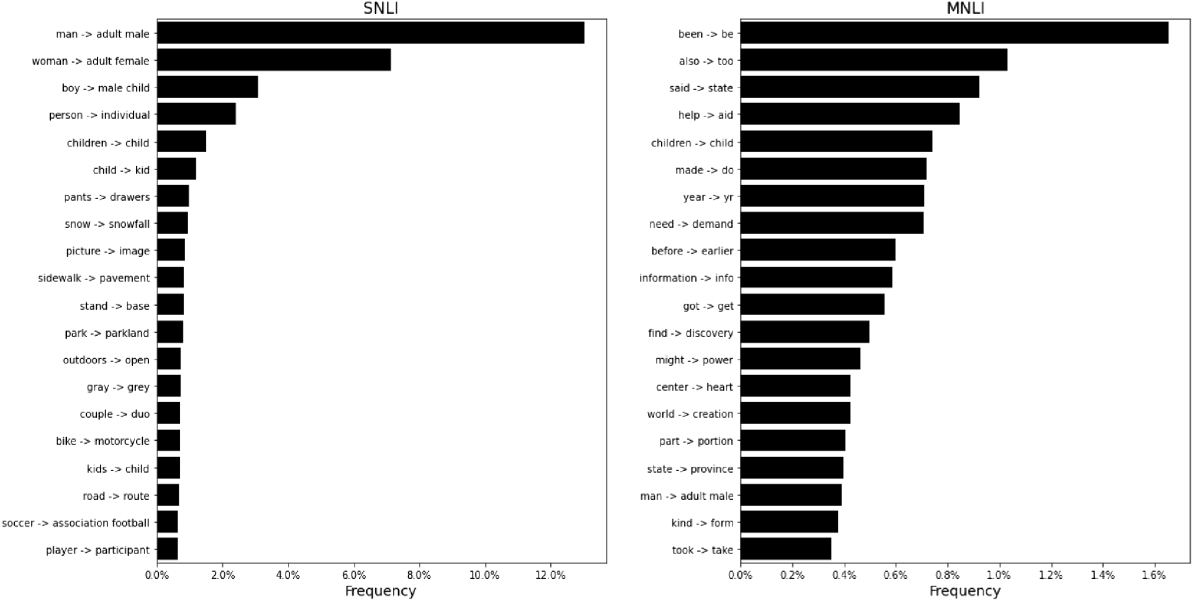
Sentence length
In both datasets, the transformation increases the size of the sentences. In the SNLI’s training data, the original text input (the concatenation of premise and hypothesis) contains, on average, $20.27$
words. After applying the transformation function, the average size of a transformed text input is
$20.27$
words. After applying the transformation function, the average size of a transformed text input is $23.61$
words (an increase of
$23.61$
words (an increase of $16.4\%$
). The numbers for the test set are similar (the average number of words in the original and transformed test set is
$16.4\%$
). The numbers for the test set are similar (the average number of words in the original and transformed test set is $21.44$
and
$21.44$
and $24.8$
, respectively). We observe a similar increase in size when we break the training data by the different labels (Table 13).
$24.8$
, respectively). We observe a similar increase in size when we break the training data by the different labels (Table 13).
Average text input length for the different partitions of the SNLI training data. The NLI labels define the partitions.
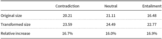
For the MNLI dataset, we also see an increase in sentence length. The original text input contains, on average, $29.93$
words. And this number increases to
$29.93$
words. And this number increases to $32.29$
words after the transformation. Breaking the dataset into labels, we also see an similar increase among all label (Table 14).
$32.29$
words after the transformation. Breaking the dataset into labels, we also see an similar increase among all label (Table 14).
Average text input length for the different partitions of the MNLI training data. The NLI labels define the partitions.
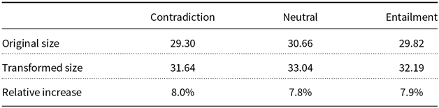
Annotation artifacts
One notorious problem associated with the classical NLI datasets is the presence of annotation artifacts. These artifacts are unintended patterns created by the crowdworkers that constructed those datasets (Gururangan et al. Reference Gururangan, Swayamdipta, Levy, Schwartz, Bowman and Smith2018). One artifact that is relevant to us is the correlation between some specific words and the NLI labels. For example, the heavy presence of negation words (no, never, and nothing) in the contradiction examples.
To assess whether the synonym substitution function adds more artifacts to the transformed dataset, we analyzed the frequency of all words mentioned by Gururangan et al. Reference Gururangan, Swayamdipta, Levy, Schwartz, Bowman and Smith(2018) in the original and transformed datasets. In both datasets, the frequency of most of the selected words remains the same after the transformation. But we have observed that the synonym substitution function both adds and removes different artifacts. The summary of these changes can be seen in Table 15.
Frequency transformation of the terms selected from Gururangan et al. Reference Gururangan, Swayamdipta, Levy, Schwartz, Bowman and Smith(2018). We only show words where the synonym substitution function has affected the frequency. By $X\% \rightarrow Y\%$
we refer to the frequency transformation of the word in the partition of the dataset (the NLI label defines the partition).
$X\% \rightarrow Y\%$
we refer to the frequency transformation of the word in the partition of the dataset (the NLI label defines the partition). $X\%$
refers to the original frequency, while
$X\%$
refers to the original frequency, while $Y\%$
represents the word frequency on the transformed dataset.
$Y\%$
represents the word frequency on the transformed dataset.
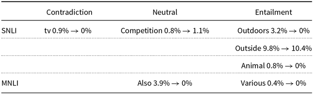
From the $30$
words mentioned by Gururangan et al. Reference Gururangan, Swayamdipta, Levy, Schwartz, Bowman and Smith(2018), we only see a change in frequency for
$30$
words mentioned by Gururangan et al. Reference Gururangan, Swayamdipta, Levy, Schwartz, Bowman and Smith(2018), we only see a change in frequency for $7$
terms. The majority of the changes are a reduction in frequency. We only see an increase in frequency for the words competition and outside (both on SNLI). It seems that the synonym substitution function only marginally changes the occurrences of annotation artifacts.
$7$
terms. The majority of the changes are a reduction in frequency. We only see an increase in frequency for the words competition and outside (both on SNLI). It seems that the synonym substitution function only marginally changes the occurrences of annotation artifacts.
Test data quality
The SNLI test set is composed of approximately $9.8$
K sentence pairs. Using the synonym substitution function, we can modify
$9.8$
K sentence pairs. Using the synonym substitution function, we can modify $92\%$
of observations. As stated before, the MNLI test set is the combination of the public matched and mismatched versions of the development set. This test set is composed of approximately
$92\%$
of observations. As stated before, the MNLI test set is the combination of the public matched and mismatched versions of the development set. This test set is composed of approximately $19.6$
K sentence pairs, and it is possible to modify
$19.6$
K sentence pairs, and it is possible to modify $91\%$
of examples. As before, we estimate the quality of the transformation on the test sets by analyzing random samples (Table 16).
$91\%$
of examples. As before, we estimate the quality of the transformation on the test sets by analyzing random samples (Table 16).
Sound percentages for the transformation function based on the WordNet database. The values were estimated using a random sample of 400 sentence pairs from the test set.
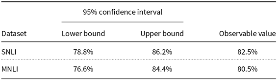
Hard cases
It is worthwhile to check some examples that challenge all the deep learning models. Here we select observations correctly predicted by the models in their original form, but, after the transformation, all the models made wrong predictions about them (regardless of how much we added modified data in the training phase).
The SNLI test set has $249$
observations of such type (
$249$
observations of such type ( $2.5\%$
of the test set). The label distribution in this sample is
$2.5\%$
of the test set). The label distribution in this sample is $45.4\%$
,
$45.4\%$
, $32.5\%$
, and
$32.5\%$
, and $22.1\%$
for the label’s entailment, neutral, and contradiction, respectively.
$22.1\%$
for the label’s entailment, neutral, and contradiction, respectively.
In Table 17, there are cherry-picked examples highlighting some interesting points. The first example shows how a wrong synonym substitution can disrupt the logical connection. The word punk is substituted for hood, this makes it hard for the model to connect to the fact in the premise 3 young adult male in hoods. The second example shows a case where the inference relationship should not be disrupted (moving ridge here has the sense of a ridge that moves across the surface of a liquid, i.e., a wave). And the third example shows how the overall context is relevant for the inference task. In this case, the contradiction arises when we compare soccer with football. In other contexts, the act of replacing soccer with association football is reasonable. But here, the fact that the word football appears both in the hypothesis and in the premise can, understandably, confuse the model.
Examples of hard cases for SNLI. Here a “hard case” is an observation that all deep learning models predict correctly in the original form, but they all make wrong predictions after the synonym substitution transformation.
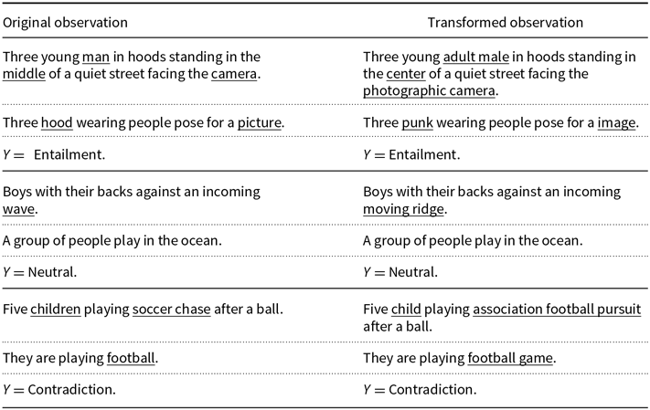
Similarly, the MNLI test set has $531$
hard cases (
$531$
hard cases ( $2.7\%$
of the test set). The label distribution in this sample is
$2.7\%$
of the test set). The label distribution in this sample is $59.9\%$
,
$59.9\%$
, $21.3\%$
, and
$21.3\%$
, and $18.8\%$
for the label’s entailment, neutral, and contradiction, respectively.
$18.8\%$
for the label’s entailment, neutral, and contradiction, respectively.
Again, Table 18 shows some interesting cherry-picked examples. The first example presents a case where a minor and acceptable text modification (the act of replacing woman with adult female) causes all models to classify the entailment instance incorrectly. The second example shows how this particular synonym substitution function can add unnecessary noise. Since we are not controlling for named entities, the organizations “Washighton Post” and “South Park” are wrongly modified. In this particular case, the association between press and Washighton Post is disrupted by the transformation, making this specific NLI observation more difficult than it should be. The third example also shows a case where context matters. Using space with the meaning of a “blank character” undermines the association between can’t remember and blank that defines this particular entailment case.
Examples of hard cases for MNLI. Here a “hard case” is an observation that all deep learning models predict correctly in the original form, but they all make wrong predictions after the synonym substitution transformation.


 Open access