


1. Introduction
The mechanisms of volcanic subsidence and basin formation associated with eruption and quick (at the geological scale), short-term (temporal) collapses of magma chambers are considered key elements to understand the evolution of volcanic areas, both in recent and ancient magma systems (e.g. Acocella, Reference Acocella2007; Gudmundsson, Reference Gudmundsson2012). Works on recent magma chamber collapses and analogue and numerical modelling provide numerous features and recognition criteria for the different typologies of this kind of structure (see, e.g. Simkin & Howard, Reference Simkin and Howard1970; Cole et al. Reference Cole, Milner and Spinks2005; Geyer & Martí, Reference Geyer and Martí2014; Gudmundsson et al. Reference Gudmundsson, Jónsdóttir, Hooper, Holohan, Halldórsson, Ófeigsson, Cesca, Vogfjörd, Sigmundsson, Högnadóttir, Einarsson, Sigmarsson, Jarosch, Jónasson, Magnússon, Hreinsdóttir, Bagnardi, Parks, Hjörleifsdóttir, Pálsson, Walter, Schöpfer, Heimann, Reynolds, Dumont, Bali, Gudfinnsson, Dahm, Roberts, Hensch, Belart, Spaans, Jakobsson, Gudmundsson, Fridriksdóttir, Drouin, Dürig, Aðalgeirsdóttir, Riishuus, Pedersen, van Boeckel, Oddsson, Pfeffer, Barsotti, Bergsson, Donovan, Burton and Aiuppa2016; Anderson et al. Reference Anderson, Johanson, Patrick, Gu, Segall, Poland, Montgomery-Brown and Miklius2019). Diagnostic structures associated with caldera collapse can be as follows: (i) radial or concentric fracture patterns (e.g. Walter & Troll, Reference Walter and Troll2001; Troll et al. Reference Troll, Walter and Schmincke2002), (ii) vertical, steep or even centrifugal (outward dipping) dip directions of faults at depth (Acocella, Reference Acocella2007) and (iii) radial flow or deformation directions in the rocks filling the basin or caldera. Some models also showed how complex tectonic patterns can occur if previous structures, usually faults, are involved (Moore & Kokelaar, Reference Moore and Kokelaar1998). Thus, the occurrence of bimodal faulting is common in these environments, often conditioned by the orientation of previous structures (Geshi et al. Reference Geshi, Ruch and Acocella2014).
However, when applied to ancient volcanic systems, these criteria related to caldera collapse present limitations (see e.g. Branney & Acocella, Reference Branney, Acocella and Sigurdsson2015). Interference between regional and volcano-related structures often occurs in these settings because of the association between crustal and/or lithospheric faults and magma plumbing systems (e.g. Christiansen et al. Reference Christiansen, Lipman, Orkild and Byers1965; Cummings, Reference Cummings1968; Best et al. Reference Best, Christiansen, Deino, Gromme, Hart and Tingey2013; Lopes et al. Reference Lopes, Caselli, Machado and Barata2015). In addition, the possibility for volcanoes (volcanic centres) to develop under different tectonic regimes, both in continental and oceanic settings, can also complicate the interpretation of structures found in ancient environments (e.g. Spinks et al. Reference Spinks, Acocella, Cole and Bassett2005; Holohan et al. Reference Holohan, van Wyk de Vries and Troll2008).
Magnetic fabrics have been long used to characterize lava flows and volcaniclastic rocks and to infer primary volcanic flows, the location of preferential pathways for magma ascent in magmatic edifices and/or deformation patterns (e.g. Tarling & Hrouda, Reference Tarling and Rouda1993; Cañón-Tapia et al. Reference Cañón-Tapia, Walker and Herrero-Bervera1996; Herrero-Bervera et al. Reference Herrero-Bervera, Cañón-Tapia, Walker and Tanaka2002; Porreca et al. Reference Porreca, Mattei, Giordano, De Rita and Funiciello2003; Bascou et al. Reference Bascou, Camps and Dautria2005; Gurioli et al. Reference Gurioli, Zanella, Pareschi and Lanza2007; Loock et al. Reference Loock, Diot, de Vries, Launeau, Merle, Vadeboin and Petronis2008; Olsanská et al. Reference Olsanská, Tomek, Chadima, Foucher and Petronis2024). When the internal fabric of volcanic rocks is not easily revealed at the outcrop or microscopic scales, the analysis of Anisotropy of Magnetic Susceptibility (AMS) can be used as a three-dimensional and continuous marker of the petrofabric in a reliable and quick way (see e.g. Cañón-Tapia, Reference Cañón-Tapia2004; Porreca et al. Reference Porreca, Mattei, Giordano, De Rita and Funiciello2003; Loock et al. Reference Loock, Diot, de Vries, Launeau, Merle, Vadeboin and Petronis2008; Simón-Muzás et al. Reference Simón-Muzás, Casas-Sainz, Soto, Gisbert, Román-Berdiel, Oliva-Urcia, Pueyo and Beamud2022). Caldera eruption dynamics and collapse mechanisms have also been analysed by means of magnetic fabrics in both outer/extra- and inner/intra-caldera (Németh et al. Reference Németh, Cronin, Stewart and Charley2009) eruptive products (e.g. Knight et al. Reference Knight, Walker, Ellwood and Diehl1986; Porreca et al. Reference Porreca, Mattei, Giordano, De Rita and Funiciello2003; MacDonald et al. Reference MacDonald, Palmer, Deino and Shen2012). Caution must be taken on these settings due to the hydrothermal activity that remained active long after the caldera collapse, which may alter the primary magnetic fabric (e.g. LaBerge et al. Reference LaBerge, Porreca, Mattei, Giordano and Cas2009; Olsanská et al. Reference Olsanská, Tomek, Chadima, Foucher and Petronis2024).
Paleomagnetism has also become a tool of increasing use for analysing volcanic deposits (both ancient and modern; Sbarbori et al. Reference Sbarbori, Tauxe, Goguitchaichvili, Urrutia-Fucugauchi and Bohrson2009; Lerner et al. Reference Lerner, Piispa, Bowles and Ort2022) for determining the age of the eruptions (Alva-Valdivia et al. Reference Alva-Valdivia, Rodríguez-Trejo, Morales, González-Rangel and Agarwal2019; Pérez-Rodríguez et al. Reference Pérez-Rodríguez, Morales, Goguitchaichvili and García-Tenorio2019), the cooling history of the different volcanic products (Tanaka et al. Reference Tanaka, Hoshizumi, Iwasaki and Shibuya2004; Paterson et al. Reference Paterson, Roberts, Mac Niocaill, Muxworthy, Gurioli, Viramonte, Navarro and Weider2010) or the palinspastic reconstruction, either of the volcanic field or the subsequent deformation underwent by the different tectonic units (Perroud et al. Reference Perroud, Calza and Khattach1991; Somoza et al. Reference Somoza, Singer and Coira1996; Chen et al. Reference Chen, Yang, Zhang, Yang, Li, Wu, Zhang, Ma and Cai2012). In the present study, paleomagnetism has been applied to constrain the age of the magnetization of the volcanic succession and to determine the degree of potential vertical-axis rotations in the Estac Basin.
The Estac Basin, in the Central Pyrenees (Figure 1a), consists of a Late Carboniferous–Permian depocentre that presents exceptional and highly varied outcrops of volcanic and volcaniclastic rocks (Gisbert, Reference Gisbert1981). In the frame of the northern Iberian margin, the Estac Basin recorded evidence of the large-scale volcanic episodes associated with the Late Permian mass extinction at the planetary scale (e.g. White, Reference White2002; Virgili, Reference Virgili2008; Saunders & Reichow, Reference Saunders and Reichow2009). Its thicker volcanic sequence and small depositional area have been interpreted as conditioned by either subsidence linked to volcanic processes (i.e. caldera collapse; Martí, Reference Martí1986; Martí & Mitjavila, Reference Martí and Mitjavila1988), extensional faulting (Saura & Teixell, Reference Saura and Teixell2006) or by the succession of different stages in which the combination of both volcanic and tectonic subsidence played a significant role (Soriano et al. Reference Soriano, Martí and Casas1996; Lloret, Reference Lloret2018). The main goals of this work are to understand the subsidence mechanisms of the Late Carboniferous–Permian Estac Basin, produce age constraints for the volcanic rocks and generate clues for determining its subsequent evolution as a basin transported in the hangingwall of a thrust sheet. To achieve these goals, we apply magnetic techniques (magnetic fabrics and paleomagnetism) and explore the resolution that they can provide to discern the triggering mechanism for the basin subsidence.
(a) Geological map of the Pyrenees and location of the Carboniferous–Permian basins from West to East: Anayet, Laspaúles, Erillcastell-Malpas, Estac and Cadí (modified from Izquierdo-Llavall et al. Reference Izquierdo-Llavall, Casas-Sainz, Oliva-Urcia and Scholger2014). (b) Geological map of the Estac Basin (Gisbert et al. Reference Gisbert, Simón-Muzás, Casas-Sainz and Soto2024) and cross-section. In the legend: G1 and Gv1 – Grey Unit. L1, L5 – Lower Red Unit. U1 and U3 – Upper Red Unit. J–P – Jurassic–Paleogene. N-Q – Neogene–Quaternary. Dashed line square indicates the zone studied in the present work and simplified in 1C. (c) Cross-section that shows the Estac basin that is cut by several thrust surfaces that are related to forelandward-rotated synformal anticlines known as têtes plongeantes.(d) Simplified sketch of the studied area including the main thrusts and slices in the Estac Basin.

2. The Estac Basin: geological context, structure and stratigraphy
The South-Pyrenean Late Carboniferous–Permian basins are arranged at present in a WNW–ESE discontinuous band along 300 km in the southern limit of the Pyrenean Axial Zone (Figure 1a). The Estac Basin is one of these Late Carboniferous–Permian basins filled with volcanic and volcaniclastic rocks, located in the Central Pyrenees (see also Soriano et al. Reference Soriano, Martí and Casas1996; Saura & Teixell, Reference Saura and Teixell2006; Lloret, Reference Lloret2018). The Estac Basin provides a good example of well-exposed volcanic and volcanoclastic deposits nearly 300 m thick, with a high variety of facies. Considering the ‘depocenter-sedimentary high’ sequence model proposed by Gisbert (Reference Gisbert1981) and Gisbert et al (Reference Gisbert, Simón-Muzás, Casas-Sainz and Soto2024), the Estac Basin represented a sub-basin of a paired system with the Erillcastell Basin, located to the west. This model describes the same subsidence pattern and distribution of depocentres and deposits exhibited by the South-Pyrenean Late Carboniferous–Permian basins, where the depocentres are regularly spaced and separated by areas or thresholds of a few kilometre where only the continental Permian red beds outcrops. Instead, Soriano et al (Reference Soriano, Martí and Casas1996) consider these two basins as independent basins. This consideration is based on the facies and thickness distribution of the volcanic rocks. The Estac Basin extends for 3 km at its central part and, in general terms, it represents a small area when compared with coeval Pyrenean basins (Cadí, Laspaúles or Anayet basins, Figure 1a).
2.a. Stratigraphy
The stratigraphy of the South-Pyrenean Late Carboniferous–Permian basins has been described and mapped by several authors (e.g. Gisbert, Reference Gisbert1981; Lloret, Reference Lloret2018; Gisbert et al. Reference Gisbert, Simón-Muzás, Casas-Sainz and Soto2024), and various syntheses, characterizations and compilations of the stratigraphy have also been made (Gretter et al. Reference Gretter, Ronchi, López-Gómez, Arche, De la Horra, Barrenechea and Lago2015; Mujal et al. Reference Mujal, Fortuny, Oms, Bolet, Galobart and Anadón2016; Mujal et al. Reference Mujal, Fortuny, Marmi, Dinarès-Turell, Bolet and Oms2018; López-Gómez et al. Reference López-Gómez, Alonso-Azcárate, Arche, Arribas, Barrenechea, Borruel-Abadía, Bourquin, Cadenas, Cuevas, De la Horra, Díez, Escudero-Mozo, Fernández-Viejo, Galán-Abellán, Gale, Gaspar-Escribano, Aguilar, Gómez-Gras, Goy Gretter, Heredia Carballo, Lago, Lloret, Luque, Márquez, Márquez-Aliaga, Martín-Algarra, Martín-Chivelet, Martín-González, Marzo, Mercedes-Martín, Ortí, Pérez-López, Pérez-Valera, Pérez-Valera, Plasencia, Ramos, Rodríguez-Méndez, Ronchi, Salas, Sánchez-Fernández, Sánchez-Moya, Sopeña, Suárez-Rodríguez, Tubía, Ubide, Valero Garcés, Vargas, Viseras, Quesada and Oliveira2019). The Cadí Basin, due to its extensive and exceptional volcanic, volcaniclastic and detrital outcrops, was considered as the reference for the definition of the Upper Carboniferous–Permian units (Grey Unit, Transition Unit, Lower Red Unit and Upper Red Unit as GU, TU, LRU and URU, respectively, see Figure 1) and the stratigraphic relationships between them (Gisbert, Reference Gisbert1981). This stratigraphic division has been extended to the rest of the rocks and deposits of other Late Carboniferous–Permian basins in the Iberian Peninsula and southern Europe (see López-Gómez et al. Reference López-Gómez, Alonso-Azcárate, Arche, Arribas, Barrenechea, Borruel-Abadía, Bourquin, Cadenas, Cuevas, De la Horra, Díez, Escudero-Mozo, Fernández-Viejo, Galán-Abellán, Gale, Gaspar-Escribano, Aguilar, Gómez-Gras, Goy Gretter, Heredia Carballo, Lago, Lloret, Luque, Márquez, Márquez-Aliaga, Martín-Algarra, Martín-Chivelet, Martín-González, Marzo, Mercedes-Martín, Ortí, Pérez-López, Pérez-Valera, Pérez-Valera, Plasencia, Ramos, Rodríguez-Méndez, Ronchi, Salas, Sánchez-Fernández, Sánchez-Moya, Sopeña, Suárez-Rodríguez, Tubía, Ubide, Valero Garcés, Vargas, Viseras, Quesada and Oliveira2019).
The Estac Basin constitutes a very narrow depositional area, in which volcanic and volcaniclastic rocks only extend 6–7 km away from its central zone (Figure 1b). In the Estac Basin, the Upper Carboniferous–Permian stratigraphic succession starts with the Grey Unit (GU) that lies unconformably on the Variscan basement (e.g. Gisbert, Reference Gisbert1981; Soriano et al. Reference Soriano, Martí and Casas1996). Its first interval (G1 part of the GU) is composed of red violet breccias that end with grey breccias of Carboniferous age (Gisbert, Reference Gisbert1981). The latter only crops out in the northernmost part of the studied area. Overlying G1, the volcanic and volcaniclastic interval (Gv1 part of the GU), Late Carboniferous–Permian in age, mainly crops out in the surroundings of the Estac village (Figure 2). In this area, the TU outcrops at the contact between Gv1 and L1, but because its outcrop is irregular, it is not continuous and difficult to record, so this unit has not been mapped (and has been included in the LRU). Upwards, the Lower Red Unit (LRU) consists of a brecciated conglomerate (L1, Figure 2a,c), followed by a package of red shales with sandy-marly levels (L5) of Permian age that only crops out in the Erta thrust sheet (Figure 1). Occasionally, the Upper Red Unit (URU) can be found in other structural units in marginal areas outside the Estac Basin. The URU consists of breccias (U1) and red shales (U3) intervals. The overlying units are the Buntsandstein, Muschelkalk and Keuper facies of the Triassic. A detailed description of the fluvial and lacustrine facies of the GU and LRU of the Estac Basin has been presented by Lloret (Reference Lloret2018).
Different views of the landscapes and outcrops of the Estac Basin: (a) General view of the dacitic lava dome (left, purplish colour) and the detrital red bed succession (right, red colour); (b) Detail of the dacitic lava dome where the flow foliation is observed; (c) Detail of the pebbles of a conglomerate in the red beds succession (LRU); (d) View of the volcaniclastic rocks with a dominant detrital component (composite deposit); (e) Detail of the composite deposit that show the characteristic texture and the dominance of lithic clasts; (f) General view of the composite deposit; (g) Detail of the ignimbrite deposit; and (h) Surge deposit were the cinerite, sandstone and volcanic layers are recognizable.

2.b. Structure
The Estac Basin, as well as the Erillcastell and Laspaúles basins to the west (Figure 1a), was incorporated during the Cenozoic Alpine compression into a sequence of southward-facing thrust sheets (têtes plongeantes, e.g. Séguret, Reference Séguret1972; Soriano et al. Reference Soriano, Martí and Casas1996; Saura & Teixell, Reference Saura and Teixell2006; Saura et al. Reference Saura, Martí, Cirés and Clariana2025, Figure 1c). The antiformal stack of the Axial Zone is formed by a highly imbricated thrust system characterized by underthrusting of the lower and younger thrust sheets (e.g. Muñoz, Reference Muñoz and McClay1992). As a consequence, the uppermost unit (the Nogueras thrust sheet) was tilted in the southern leading edge of the antiformal stack, showing downward-facing structures (Séguret, Reference Séguret1972). They are characterized by hangingwall anticlines completely overturned and include Variscan basement rocks, the Upper Carboniferous–Permian stratigraphic succession and the Triassic cover (Figure 1c). Their hangingwalls (older materials) are located south of the thrust surfaces, and their footwalls (younger materials) are located to the north of these thrust surfaces. From north to south, the main Alpine thrust sheets affecting the Estac Basin (Figure 1d) are (Saura & Teixell, Reference Saura and Teixell2006): (i) Orri, (ii) Erta, (iii) Arcalís-Estaén, (iv) Freixe and (v) Castells. The Upper Carboniferous–Permian volcanic and volcaniclastic rocks crop out in the first three thrust sheets (Figure 1). The most continuous basin infill, with a maximum thickness of nearly 300 m, is observed along a monocline located in the Erta thrust sheet (Gisbert et al. Reference Gisbert, Simón-Muzás, Casas-Sainz and Soto2024). The hangingwall of this thrust sheet shows different strikes of bedding because it is gently folded by a steeply plunging anticline (Figure 1; Soriano et al. Reference Soriano, Martí and Casas1996; Saura & Teixell, Reference Saura and Teixell2006; Gisbert et al. Reference Gisbert, Simón-Muzás, Casas-Sainz and Soto2024). The Permian red beds only crop out in the Erta thrust sheet, to the east, while red beds in Buntsandstein facies (Triassic age) appear in all the thrust sheets mapped in the area (Figure 1b–d), consistently with the extensive sedimentation of the Triassic red beds in relation to previous stages. According to the geometrical relationships with bedding, it can be interpreted that the thrust surfaces and the main extensional fault located at the southern border of the basin (not exposed at present) were initially dipping towards the north, and were subsequently tilted during the emplacement of the underlying thrust sheets. This also occurs in the other Late Carboniferous–Permian basins in the Southern Pyrenees (Cadí and Erillcastell basins; Saura & Teixell, Reference Saura and Teixell2006).
3. Methodology
3.a. Structural analysis
Orientations of structural data, such as bedding and fault plane attitudes, and orientation of slickenline striations, joints and cleavage planes, were collected in the AMS sampling sites with a magnetic compass and a digital tablet with the FieldMove app (Midland Valley Exploration). Microstructural observations of oriented rock samples and thin-sections were also done. Establishing the relationship between structural markers and the orientations of the magnetic ellipsoids allows us to determine the fabric origin: either (i) a primary magnetic fabric related with the original orientation of the minerals during their deposit or formation, or (ii) a secondary magnetic fabric generated after the tectonic reorientation of the mineral assemblage or by the neoformation of minerals due to hydrothermal alteration processes (see e.g. Hrouda et al. Reference Hrouda, Burianek and Krejcí2020) under the prevailing tectonic regime in the studied zone.
3.b. Sampling
A total of 32 sites, totalling 473 specimens, were sampled for the paleomagnetic and magnetic fabric characterization of the Upper Carboniferous–Permian volcanic and volcanoclastic rocks of the Estac Basin (Tables 1 and 2, Figure 3).
Studied sites in the volcaniclastic succession from the E–W transect (red squares) and the N–S transect (green squares). The main faults set, and the two folds present a NNW–SSE trend.

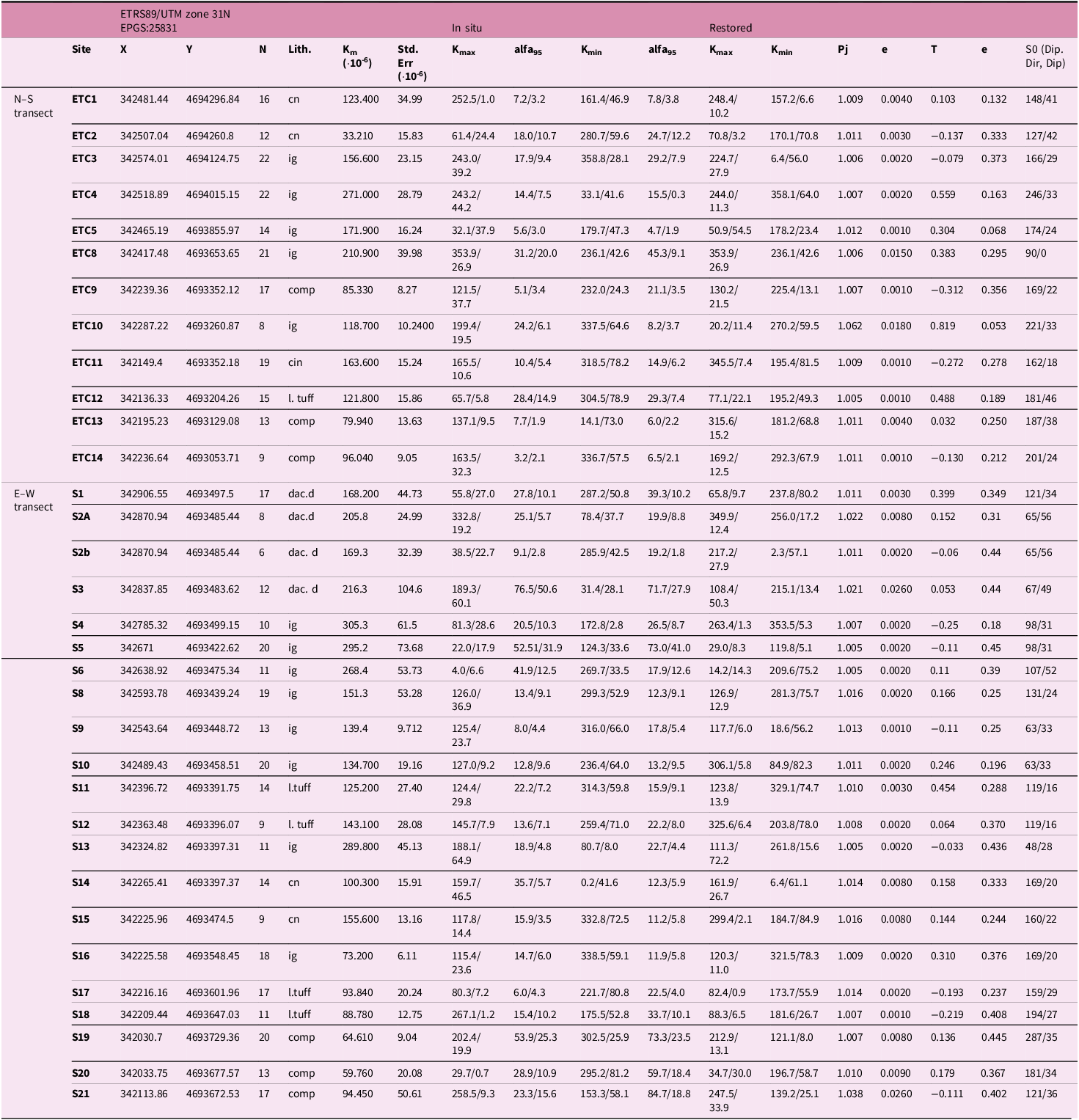
Summary of magnetic fabric data. Label of the site, coordinates X and Y in ETRS89/UTM zone 31N EPGS:25831; N: number of specimens; Lith: studied lithology, cn: cinerites, ig: ignimbrites, comp: composite deposit, dac. d: dacitic lava dome, l. tuff: lithic tuff; Km: mean magnetic susceptibility value per site and standard deviation in the next column. Kmax and Kmin (trend and plunge) of the magnetic lineation and of the pole to the magnetic foliation (Jelinek, Reference Jelinek1977) in situ and after the tectonic correction and the α 95 of each one; α 95: major and minor semi-axes of the 95% confidence ellipse (Jelinek, Reference Jelinek1977); Pj: corrected anisotropy degree (Jelinek, Reference Jelinek1981); T shape parameter (Jelinek, Reference Jelinek1981); e: standard deviation; bedding data plane expressed in dip direction/dip

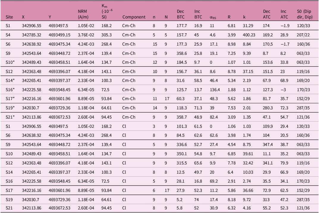
Paleomagnetic data at site level of the 1) low-temperature component (Cl) in the upper table; 2) high-medium component (Cm-Ch) in the lower table; both from the volcanic and volcaniclastic rocks. Sampled section and name of the site, coordinates (X and Y in ETRS89/UTM zone 31N EPGS:25831), n: number of specimens where a paleomagnetic component could be isolated (Cm, Ch or both and Cl). See Supplementary table for additional details; N: number of specimens; site-mean NRM value, Km: site-mean susceptibility value, Declination (Dec) and Inclination (Inc) before (BTC) and after (ATC) tectonic correction; α 95 and k are the statistical parameters of a fisherian distribution (Fisher, Reference Fisher1953); S0: bedding plane (dip direction and dip). Data in sites with * did not pass the quality thresholds and are not considered for the mean directions calculations (see supplementary table S1 for details)

The sampled sites are distributed along two transects (Figure 3): (i) an E–W transect, perpendicular to the overall strike of bedding (20 sites), and (ii) a N–S transect, sub-parallel to the strike of the bedding planes (12 sites). Sites were homogeneously distributed along the stratigraphic succession (average spacing between sites around 15 to 20 m, see Figure 3). Samples were obtained either as oriented cores with a gasoline-powered drill or as oriented blocks with manual extraction tools. All samples were oriented in situ with a magnetic compass and positioned with a GPS. Sun azimuths were also recorded to check potential deviations of magnetic compass measurements. Additionally, surficial mean magnetic susceptibility values were measured with a KT-20 hand-held susceptometer. Oriented cores and blocks were cut to 2.1 cm-long and 2.5 cm-diameter standard cylinder specimens and 2 cm-edge standard cube specimens, respectively, with a radial saw (non-magnetic steel). Between nine and 20 cylindrical specimens (one to three specimens per core, 10 cores on average per site, samples initial S) and between nine and 22 specimens cubes obtained from a number of oriented blocks between three and five (samples initials ETC) were obtained in each site.
3.c. Analysis of RT-AMS
The analysis of the AMS at room temperature (RT-AMS) was carried out in specimens from the 32 sampling sites. It was done using a Kappabridge KLY-3S susceptometer (AGICO Inc., Czech Republic) in the 15 manual positions procedure at the Magnetic Fabrics Laboratory of the University of Zaragoza (Spain).
AMS is a technique based on the spatial variation of the magnetic susceptibility (k) within a sample of rock. This magnetic property is defined as the capacity of minerals to acquire a magnetization when exposed to a low-intensity magnetic field. When that field is applied in different orientations around a standard rock specimen, the magnetization induced in the rock may be different in those different orientations, depending on the distribution and orientation of the mineral grains within the specimen (see e.g. Tarling & Hrouda, Reference Tarling and Rouda1993). Magnetic susceptibility is dimensionless in SI units and is characteristic of each material, helping to relate the induced magnetization acquired (M) when exposed to an external field of certain intensity (H), expressed as
 $$\overrightarrow M = k \cdot \overrightarrow H $$
. This property can be described mathematically as a second-rank symmetric tensor and geometrically as an ellipsoid with three orthogonal principal axes of magnetic susceptibility, K
1 or K
max > K
2 or K
int > K
3 or K
min.
$$\overrightarrow M = k \cdot \overrightarrow H $$
. This property can be described mathematically as a second-rank symmetric tensor and geometrically as an ellipsoid with three orthogonal principal axes of magnetic susceptibility, K
1 or K
max > K
2 or K
int > K
3 or K
min.
The magnetic susceptibility (k) is the sum of the contributions of all the mineral grains present in the sample (diamagnetic, paramagnetic or ferromagnetic s.l.). The geometry of the magnetic susceptibility ellipsoid can be characterized by the orientation of its axes and three scalar parameters (Jelinek, Reference Jelinek1981): (1) the mean magnetic susceptibility (Km or Kmean), expressed as Km = (K 1 + K 2 + K 3)/3, (2) the corrected anisotropy degree (Pj), expressed as Pj = exp√2[(µ1 − µm)2 + (µ2 − µm)2 + (µ3 − µm)2], and (3) the shape parameter (T), expressed as T = 2µ 2 − µ 1 − µ 3, where μ = ln K 1, μ = ln K 2, μ = ln K 3 and µ1 − µ3μm = (μ 1 + μ 2 + μ 3)/3. Another two relevant parameters related to the magnetic susceptibility ellipsoid, which allow to distinguish between oblate, triaxial and prolate (s.l.) ellipsoid geometries, are as follows: (1) the magnetic lineation, that is the cluster of the K 1 axes expressed as L = K 1/K 2 and (2) the magnetic foliation, the plane whose pole is the cluster of K 3 axes expressed as F = K 2/K 3.
3.d. Paleomagnetism
After the magnetic fabric analysis, nine specimens from 11 sites (S1, S4, S6, S9, S10, S12, S14, S16, S17, S19 and S21, Figure 3 and Table 2) were selected to perform a paleomagnetic study. These sites cover the entire range of Km values observed in the studied rocks and the whole Upper Carboniferous–Permian volcanic and volcaniclastic succession. The paleomagnetic study was carried out in the Pacific Northwest Paleomagnetism Laboratory of the Western Washington University (Bellingham, WA, USA).
3.d.1. Alternating field (AF) and thermal demagnetizations
To recognize the best demagnetization routine, two pilot specimens per site were selected: one of the specimens was demagnetized with steps of alternating fields (AF) of increasing intensity up to 120 mT (12 steps: 5, 10, 15, 20, 25, 30, 40, 50, 60, 80, 100 and 120 mT) in a DTech D-2000 AF demagnetizer and the other one was thermally demagnetized (Th) in steps from room temperature up to 680°C (17 steps: 150, 200, 250, 300, 330, 400, 425, 450, 500, 525, 550, 580, 600, 620, 640, 660, 680°C) with a TD48-DC thermal demagnetizer. The remaining field after each demagnetization step was measured using a Superconducting Rock Magnetometer (2-G Enterprises). The directional results for the studied rocks were displayed on Zijderveld diagrams (Zijderveld, Reference Zijderveld, Collinson, Runcorn and Creer1967), and the magnetic directions were analysed using the software Remasoft 3.0 (Chadima & Hrouda, Reference Chadima and Hrouda2006).
3.d.2. Low-temperature demagnetizations
To evaluate a potential effect of multidomain (MD) magnetite grains in the paleomagnetic results, a low-temperature (LT) demagnetization routine was performed in selected specimens (see e.g. Borradaile et al. Reference Borradaile, Lucas and Middleton2004), as a treatment prior to the regular AF or Th demagnetizations described above.
Previous studies showed the effectiveness of the LT-demagnetization routine to unblock the viscous magnetization that MD magnetite grains may easily acquire, resulting in a potential overprint of the high unblocking temperature remanence carried by single domain grains (Warnock et al. Reference Warnock, Kodama and Zeitler2000 and references therein). A total of 14 specimens were submerged in liquid nitrogen (77 K) in two cooling cycles of one hour each. Between cycles, specimens were brought back to room temperature in a magnetically shielded space, and NRM measurements were done in the 2-G cryogenic magnetometer after each step. Then, the AF of Th demagnetization routine was performed normally as in the rest of the specimens.
3.e. Magnetic mineralogy
Three types of analysis at room temperature were carried out in samples from 11 sites from the E–W transect (S1, S4, S6, S9, S10, S12, S14, S16, S17, S19 and S21, Table 1) to determine their magnetic mineralogy: (i) temperature-dependent magnetic susceptibility curves, (ii) hysteresis loops and (iii) isothermal remanent magnetization (IRM) acquisition and backfield curves. The aim of these experiments was to recognize the magnetic mineralogy responsible for the magnetic susceptibility and the natural remanent magnetization (NRM).
Temperature-dependent magnetic susceptibility curves were carried out in a KLY-3S Kappabridge susceptometer combined with a CS-3 furnace (temperature range between 40 and 700°C). Data were processed with the software SUSTE (AGICO, Inc., Czech Republic) and represented with the software Cureval8 (Chadima and Hrouda, Reference Chadima and Hrouda2012), taking into account the correction of the free furnace (measure of the CS3 without the sample) and the normalization of the susceptibility values to a standard-volume specimen by calculating the density and the mass of the powdered sample. The hysteresis loops record the induced magnetic moment acquired by a sample subjected to a magnetic field of varying intensity (from 0 to 1 T). The IRM acquisition curves register the remanent magnetization a sample can acquire under an increasing intensity field (up to 1 T). Both experiments were performed in a Micromag 3900 Vibrating Sample Magnetometer (VSM, Princeton Measurements Corp.). All analysed samples were powdered in a ceramic mortar (0.3–0.6 g per sample) and deposited in a diamagnetic gelatine capsule within a diamagnetic plastic tube in the VSM for their analysis. All the magnetic property analyses were carried out in the Pacific Northwest Paleomagnetism Laboratory of the Western Washington University (Bellingham, WA, USA).
4. Results
4.a. Identification of lithological types in the volcaniclastic rocks
To identify the different lithological types in the volcanic and volcaniclastic rocks, we followed White & Houghton’s (Reference White and Houghton2006) classification. The three main groups in which the volcaniclastic rocks were classified are pyroclastic, autoclastic and composite deposits. In the pyroclastic deposits identified in the studied area, a grain-size gradation was considered: (i) cinerite (fine tuff), (ii) lapilli tuff and (iii) ignimbrite deposit (Figures 2g and 4). In the latter, juvenile clasts with fiamme structures are recognizable. Within the autoclastic deposits, the (i) volcanic conglomerate or breccia and (ii) lava dome deposits were distinguishable. The first one is constituted by clasts made of fragments of lava (rounded or angular) mixed with some lithic clasts; the second presents a lava texture, but the morphology of the deposit in the outcrop is dome-like, indicating a short magma flow path (Figure 2b). In the composite deposits (Figure 2d–f), the clasts formed by mingling of magma with a clastic host rock, or the clasts formed by the incorporation of lithic debris into a magma (composite clasts), clearly dominate (White & Houghton, Reference White and Houghton2006) the petrofabric. Surge deposit (Figure 2h) is a recurrent genetic term in the present work, but it does not refer to the lithological classification; instead, it is only used in the field description, where grain-size gradation is clearly noticeable, since this helps to understand the depositional mechanism of the lithologies present in the basin.
(a) Thin section of the volcaniclastic and volcanic rocks, one half in PPL: Plane polarized light and the other half in XPL: Cross polarized light. (b) Sections of the oriented cylinder specimens: the different textures are recognizable.

The ignimbrites dominate in the central and northern sectors of the Estac Basin. The lithic tuffs and composite deposits are dominant in its southern zone. Lithic tuffs and cinerites also appear intercalated within the ignimbrite deposits. In the dacitic lava dome, quartz and feldspar grains are recognizable and dominate the mineral assemblage, embedded in a glass matrix (Figure 4a, see sample S2-2 and Figure 4b, see sample S3). At the outcrop scale and in hand specimen, the colour of the matrix is purplish. The andesitic ignimbrites present feldspars, plagioclases and mafic minerals with flow bands and punctually fiamme structures (Figure 4a, see S6-1 and S5-2, and Figure 4b see S13). The grain-size criterion was used for the classification of the cinerites (Figure 4b, S15) and lithic tuffs (Figure 4a, see S17 and Figure 4b, see S11). The composite deposits are characterized by a clear dominance of lithic clasts with a scarce (Figure 4b, see S21) to abundant proportion of volcanic components (Figure 4b, ETC14).
The petrographic observations reveal a well-developed flow orientation in the volcanic (especially in the ignimbrites) and volcaniclastic rocks. The main phenocrystals (Figure 4) in the volcanic portion of the studied rocks are plagioclase and opaque minerals, and also pyroxene and amphibole in minor proportion, and carbonate and silicic cement. Some of the main phenocrystals are pseudomorphs presumably of plagioclase, amphibole and/or pyroxene replaced by carbonates, opaque and other secondary minerals. The microcrystalline matrix is composed of plagioclase, opaque minerals and alteration products like carbonate cement and vacuoles filled by opaque minerals. The main phenocrystals in the detrital portion of the studied rocks are mainly quartz, feldspars and micas.
4.b. Structural study
Bedding dips present average values of 30° towards the SE in both the Upper Carboniferous–Permian volcanic/volcaniclastic rocks, as well as in the overlying detrital Permian and Triassic red beds close to the contact with the volcanic rocks (Figures 3 and 7). Bedding dips steeper than 50° have not been considered as representative, as they are generally linked to local fault zones. Bedding planes define a monoclinal panel with a gentle anticline whose axis is 134/27 (trend/plunge) and other shorter wavelength folds (Figure 7). Towards the E, the detrital red beds describe a syncline subparallel to the large-scale anticline.
Structural data (bedding, fracture and fault planes) represented in stereoplots (lower hemisphere) with rose diagrams representing strikes, site by site and projected along the stratigraphic log on the left (sites from the E–W transect in black colour, sites from the N–S transect in green colour). In the upper part, structural data are plotted together by type. The changes in orientation and dip in bedding planes describe a syncline (fold axis: 134/27, red dot). Three main fracture sets, trending N–S, NNE–SSW and E–W, are present. Fault planes with associated slickensides (red dots) show that the main set is the one trending E–W.

More than 450 fractures and faults were measured in the study area (Figures 1 and 3). Two sets of fractures and faults are distinguishable (both at the outcrop and the cartographic scale), oblique to the main structural trend of the basin: (i) a dominant NW–SE striking set, and (ii) a dominantly NE–SW to ENE–WSW striking set. Additionally, an E–W fracture set is also present in the volcanic/volcaniclastic succession. (Figure 7). Faults with associated slickenlines mostly strike or trend to the NW–SE, changing to an E–W trend in the upper part of the basin filling (Figures 3 and 7). N–S and NE–SW sets are also recognized locally in the upper part of the stratigraphic section of the N–S transect. Slickenlines indicate strike-slip, normal and oblique movements (Figure 7). It is worth highlighting the absence of penetrative deformation in all analysed sites. At the cartographic scale, the NNW–SSE fault set is difficult to recognize.
4.c. Magnetic mineralogy
All temperature-dependent magnetic susceptibility curves are irreversible, i.e. the heating and cooling paths are not overlapped. This fact points towards the neoformation of magnetic minerals during heating in all sampled lithological types. In most analysed samples, the heating curves present a slightly concave hyperbolic shape at the lower temperatures, indicating a significant paramagnetic contribution. Most curves show an abrupt decay of magnetic susceptibility at 580°C that suggests the presence of magnetite, except for curves S1-5B and S19-5 which points toward the presence of haematite (Figure 5).
Temperature-dependent susceptibility curves (40 to 700 °C) for the seven analysed samples. Heating run (in red) and cooling run (in blue) show the non-reversibility of curves. (b) Enlargement of the heating curves: the decay at 580 °C is observed in samples S9 and S4; the decay around 700 °C is observed in sites S1 and S19.

The presence of paramagnetic minerals is corroborated by the hysteresis loops in all samples except for S1-10b. IRM acquisition curves show saturation of the remanent magnetization (slope of the curve is zero) under intensities way below the maximum applied field of 1T, ruling out the presence of high coercivity ferromagnetic minerals in the samples (Figure 6).
Representative hysteresis loops before and after paramagnetic slope adjustment (magnetic saturation, coercivity and magnetic remanence values are reported in each case), and IRM acquisition curves together with the backfield (coercivity of the remanence obtained from backfield results).

Hysteresis loops in the same specimens also point to the presence of a low coercivity ferromagnetic fraction in the samples. However, the slope of the two halves of each loop remains positive (under induced magnetization), indicating the likely presence of paramagnetic minerals in the mixture. These results permitted applying a paramagnetic slope adjustment of the hysteresis loops that allows for a better visualization of the hysteresis parameters of the ferromagnetic fraction detected (reported in Figure 6 and Supplementary material 5): magnetic saturation (Ms), magnetic remanence (Mr), coercivity (Hc) and (Hcr) remanence coercivity. Only sample S1-10b remained undersaturated at 1T, as observed by the positive slope at high fields in its IRM acquisition curve (Figure 6), which points towards the presence of a ferromagnetic mineral with a higher coercivity (such as haematite). The backfield curves point towards a ferromagnetic mineral with low coercivity that saturates around 0.2 T except in sample S1, which does not reach saturation at 1 T.
4.d. Analysis of RT-AMS
The mean magnetic susceptibility (Km) for all sites is 150.6 × 10⁻⁶ SI, ranging between 33 × 10–6 SI (site ETC2, std. dev. 15.83 × 10⁻⁶) and 305 × 10–6 SI (site S4, std. dev. 61.5 × 10⁻⁶). Km values are low compared to other volcanic and volcaniclastic rocks from other South-Pyrenean Late Carboniferous–Permian basins (see Simón-Muzás et al. Reference Simón-Muzás, Casas-Sainz, Soto, Gisbert, Román-Berdiel, Oliva-Urcia, Pueyo and Beamud2022). The Km values measured with the hand-held susceptometer are between 50 and 100 × 10–6 SI, lower than the Km values measured from standard specimens in the laboratory. This reduction is generally related to the surficial alteration that affects the volcanic rocks and to the presence of irregular surfaces that decrease the contact area with the field instrument sensor.
The mean corrected anisotropy degree (Pj) is 1.013, with a minimum value of 1.005 (site S5, std. err. 0.002) and a maximum value of 1.062 (site ETC10, std. err. 0.018). The observed Pj values under 1.1 are homogeneous along the stratigraphic log and laterally in each cross-section. Only sites ETC10 and S21 do not follow this general trend and present values above 1.030 (1.038 and 1.062 respectively, std. err. 0.026 and 0.018, respectively). The mean shape parameter (T) is 0.102, ranging between –0.312 (site ETC9, std. err. 0.356) and 0.819 (site ETC10, std. err. 0.053). No relationship is observed between values of these parameters, Km, T and Pj, and the lithology (Figure 8). The parameter T varies between prolate, triaxial and oblate geometries along the stratigraphic log. This variability is also observed in the orientation of the magnetic lineation (K1) after tectonic correction (Figure 8).
Magnetic scalar parameters of the studied sites from the E–W (black colour dots) and N–S (green colour dots) transects, plotted along the stratigraphic log. Km: mean magnetic susceptibility value (site scale), unfilled dots, susceptibility measured withy the KT20 hand-hold susceptometer and filled dots, magnetic susceptibility measured in the laboratory with the Kappabridge susceptometer; T: shape parameter (site mean); Pj: corrected anisotropy degree (site mean). T and Pj based on Jelinek (Reference Jelinek1977); and Kmax direction: magnetic lineation direction (from 0 to 180°), site mean axis after tectonic correction.

Along the E–W transect, the magnetic fabric results show some particularities (Table 1, Figures 9 and 11): magnetic fabrics obtained in the volcanic conglomerate and breccia located at the bottom of the stratigraphic log present a chaotic and scattered distribution of the magnetic ellipsoid axes, consistent with their origin and texture. The volcanoclastic rock intervals (including breccias, microconglomerates, sandstones, cinerites and tuffs) show K3 mean axes perpendicular to the bedding planes (e.g. sites S8, S15, Figure 9) or in a girdle with the K2 axes (e.g. site S18; Figure 9). The ignimbrite intervals also show K3 mean axes perpendicular to the bedding plane, except for sites S4 and S13 where axes switch between K2 and K3 and between K1 and K3 (Figure 9). The dacitic ignimbrite at the top of the series shows a poorly defined magnetic susceptibility ellipsoid, and site S2 presents an exchange between the K2 and K3 axes. Sites S3, S4 and S5 were sampled in a strongly fractured and faulted interval; for sites S3 and S5, the scattered results could be related to the influence of these local structures.
AMS ellipsoids (in situ) obtained for each sampling site with their confidence ellipses (Jelinek, Reference Jelinek1977) from the E–W transect along the stratigraphic log. The projection of the bedding planes and their pole is also represented in situ. Classified according to their lithology: ignimbrite, cinerite, volcanic conglomerate/breccia and dacitic lava flow.

In the N–S transect, lateral changes of the magnetic fabric can be recognized within the same rock interval (Table 1, Figures 10 and 11). To the south, volcanoclastic and pyroclastic deposits dominate (conglomerates in sites ETC9, ETC13 and ETC14, and cinerites in ETC10, ETC11 and ETC12). Their magnetic fabric follows the same pattern as in the E–W transect, with the K3 axes perpendicular to the bedding plane or distributed in a girdle with the K2 axes that are perpendicular to bedding (e.g. site ETC9). From the centre to the northern basin margin, the ignimbrite deposits are the main lithology (sites ETC3, ETC4, ETC5 and ETC8) and show similar orientations as in the E–W transect. In site ETC5, an exchange between the K1 and K3 axes is observed. Sites ETC1 and ETC2 are in the northern basin border and correspond to cinerite intervals located above the volcanic conglomerate/breccias at the base of the stratigraphic succession. The distribution of the magnetic ellipsoid axes in sites ETC1 and ETC2 seems to be more related to compressive magnetic fabrics: the K1 axes are parallel to the structure (i.e. the strike of thrusts), and additionally, in the ETC1, the orientation of K3 axes is compatible with a tectonic foliation in the studied zone (Figure 11).
AMS ellipsoids in situ obtained for each sampling site with their confidence ellipses (Jelinek, Reference Jelinek1977) from the N–S transect along the stratigraphic log. The projection of the bedding plane and its pole is represented in situ. Classified according to their lithology: ignimbrite and cinerite.

a) Geological map of the volcanic and volcaniclastic succession of the Estac Basin. Magnetic lineation (left picture, K1 axis) and magnetic foliation (plane perpendicular to the K3 axis) of the magnetic fabric results for each studied site in situ; b) Magnetic fabrics stereoplots (lover hemisphere) at specimen level of the 33 studied sites that show the K1 (magnetic lineation) and the K3 (pole of magnetic foliation) in situ and after the tectonic correction. Kamb contours in standard deviation in red and blue colour ramp.

In summary, most sites show the magnetic foliation subparallel to bedding independently of their lithology. With respect to the magnetic lineation, two preferred directions are observed: a prominent WNW–ESE direction, which coincides with the orientation of the magnetic lineation observed in the coeval Cadí and Laspaúles basins (Izquierdo-Llavall et al. Reference Izquierdo-Llavall, Casas-Sainz, Oliva-Urcia and Scholger2014; Simón-Muzás et al. Reference Simón-Muzás, Casas-Sainz, Soto, Gisbert, Román-Berdiel, Oliva-Urcia, Pueyo and Beamud2022), and a secondary maximum oriented N–S (Figures 10 and 11).
4.e. Paleomagnetism
The mean NRM per site ranges between 6.34 × 10⁻⁵ and 3.76 × 10⁻² A/m, with the mean value being 4.90 × 10⁻³ A/m. The NRM values are not related to the lithology; the volcanic rocks do not show the highest NRM intensities, and the volcanoclastic rocks with a greater concentration of sedimentary particles do not present the lowest NRM intensities either, contrary to what has been observed in previous studies in other South-Pyrenean Late Carboniferous–Permian basins (e.g. Simón-Muzás et al. Reference Simón-Muzás, Casas-Sainz, Soto, Pueyo, Beamud and Oliva-Urcia2023).
In most demagnetized specimens (see Supplementary material 4, 6 and 7), two to three paleomagnetic components were isolated (two in the specimens demagnetized by AF, Cm and Ch) and two or three (Cl, low temperature, Cm, intermediate temperature, and Ch, high temperature) in those demagnetized thermally. Both Cm and Ch components have generally overlapped directions, and in some specimens, they share part of the unblocking temperature ranges (see Supplementary Table S1 for details), so they are considered the same component at the site scale. Acquisition mechanisms in these volcanic and volcaniclastic rocks are certainly complex, due to multiple factors: cooling rate of the magma, different depositional processes involved, mixture between volcanic and detrital rocks, and secondary hydrothermal alteration.
The site mean α 95 values of the paleomagnetic directions (Fisher, Reference Fisher1953) were used to establish a quality threshold and sites with α 95 above 30° were rejected. Additionally, mean NRM values under 1 × 10⁻⁴ A/m were discarded. The k values were considered to establish when a paleomagnetic direction is random or not: sites with k > 10 are non-random. At the specimen level, paleomagnetic components with a Maximum angular deviation (MAD) above 16 were not considered. For thermally demagnetized specimens in which both Cm and Ch could be isolated, only the one with the lowest MAD was considered for the site mean (see Supplementary table S1 for details). No composite deposits have passed the quality threshold; therefore, this lithology is considered to be unfavourable for the paleomagnetic study.
The LT demagnetization routine (see Supplementary material 4) in 14 specimens decreased the intensity of the NRM by a percentage between 34 and 0.44. From this result, we can suggest that the presence of MD magnetite in the studied samples varies between sites. No clear relationship between the reduction in NRM intensity and the diverse lithology of the specimens subjected to the protocol can be established. In any case, our sample size (14 specimens) is too small to attempt any further discussion about MD magnetite concentration in the studied rocks. However, the results obtained from the standard demagnetization protocol applied to these specimens did not show a noticeable improvement in terms of the definition of the paleomagnetic components. For that reason, the technique was not applied to the rest of the analysed specimens.
Three paleomagnetic components have been isolated in the thermally (Th) demagnetized specimens (Table 2 and Supplementary materials 2, 6 and 7):
-
Cl: a LT component is defined between 300 and 400°C. In some specimens, it occasionally reaches up to 440–450°C.
-
Cm: an intermediate temperature component is defined between 300–400 and 540–520°C. This component is the least common, being characterized in only 43 specimens. The range of temperatures in which it can be defined is also the most variable.
-
Ch: a high temperature component is defined between 500–540 and 560–580°C. It occasionally starts at a lower temperature.
Two paleomagnetic components were isolated in the specimens demagnetized by AF (Table 2 and Supplementary materials 6 and 7):
-
Cl: a low AF component is defined between 1.5–15 and 20–30 mT.
-
Ch-Cm: a high-medium AF component is defined between 15–60 and 100–120 mT (variable limits range).
The diagrams of the normalized intensity of NRM versus temperature show four different behaviours (see Supplementary materials 4): (i) an abrupt decay before 130 °C (S9, S10, S12, S14, S16, S17, S19) and a secondary decay around 580 °C; (ii) a prolongate decay that starts at 400 °C and finishes at 580 °C and after that, the magnetization value increases; (iii) an abrupt decay at 580 °C (S4 and S6) that starts at 400 °C and not complete demagnetization at 600 °C (S1).
5. Interpretation and discussion
5.a. Volcanic paleoflow directions, paleomagnetic data and fracture pattern in the Late Carboniferous–Permian Estac Basin
The AMS results point to a primary origin of the magnetic fabric in most sites, taking into account the subparallel orientation of the magnetic foliation (i.e. plane perpendicular to Kmin axes, Figures 9 and 10, Supplementary material 1) to bedding. Moreover, we interpret that the magnetic lineation reflects the primary volcanic flow because of the absence of penetrative deformation that could reorient the magnetic lineation and generate secondary magnetic fabrics. The pattern of interpreted volcanic paleoflow directions in map-view is shown in Figure 11. A strong dominance of the WNW–ESE to NW–SE directions and a secondary maximum along a N–S direction are clearly seen. Additionally, the magnetic foliation planes also show a bimodal distribution. It is worth highlighting the absence of a radial pattern regarding the direction of the observed volcanic paleoflows that could indicate the dominance of intra- and/or extra-caldera deposits (Németh et al. Reference Németh, Cronin, Stewart and Charley2009).
Related to the paleomagnetic data and independently of the demagnetization technique, the mean Cl component has been isolated and passes the quality criteria in ten out of the eleven studied sites. This Cl component has a declination of 1.5° and an inclination of 61.4° before tectonic correction (N = 10, R = 10.06, k = 10.65, α 95 = 14.7°; Table 2 and Figure 13). It has been interpreted as a viscous component corresponding to the recent or current Earth’s magnetic field direction for in situ coordinates. The Cm-Ch component (Figures 12 and 13) presents good quality (MAD < 16) in individual paleomagnetic directions at five sites (out of 11), whereas in the other six sites, this component shows a random distribution at the site level (sites S10, S14, S16, S17, S19 and S21; see Supplementary material 2) and a mean paleomagnetic component could not be accurately defined. In five sites (S1, S4, S6, S9 and S12), the individual paleomagnetic directions at the site level and the site average are of good quality and well-clustered (individual α 95 values per site range between 4.6° and 15.6°). At the site level (Figure 13), the resulting mean paleomagnetic direction (considering data from S9 in its antipodal reverse polarity) has a declination of 170.6° and an inclination of 6.5° after bedding correction (N = 5, R = 4.69, k = 13.02 and α 95 = 22.0°). This paleomagnetic direction coincides with the Late Carboniferous–Permian reference for the studied location (D = 166, I = −9; Oliva-Urcia et al. Reference Oliva-Urcia, Pueyo, Larrasoaña, Casas, Román-Berdiel, Van der Voo and Scholger2012; Simón-Muzás et al. Reference Simón-Muzás, Casas-Sainz, Soto, Pueyo, Beamud and Oliva-Urcia2023 and references therein), pointing to the absence of important vertical-axis rotations despite the structural complexity of the study area.
Medium-high temperature paleomagnetic component and α 95 confidence cone for each site (Fisher, Reference Fisher1953), in situ and after tectonic correction. Dec: declination, Inc: inclination and α 95 : α 95 confidence values. Reference direction D/I = 166, −9 from Oliva-Urcia et al. (Reference Oliva-Urcia, Pueyo, Larrasoaña, Casas, Román-Berdiel, Van der Voo and Scholger2012).

Paleomagnetic results of the medium-high (upper row of stereoplots) and low-temperature (lower row of stereoplots) component at site level: in situ (left) and after the tectonic correction (right; See all the paleomagnetic results in Table 2 and Supplementary material). The resulting mean paleomagnetic direction (considering data from S9 in its antipodal reverse polarity). Before transposition, see the small stereogram above. Permian reference direction D/I = 166, −9 from Oliva-Urcia et al. (Reference Oliva-Urcia, Pueyo, Larrasoaña, Casas, Román-Berdiel, Van der Voo and Scholger2012).

This paleomagnetic direction coincides with the mean declination and inclination for the Late Carboniferous–Permian interval (Oliva-Urcia et al. Reference Oliva-Urcia, Pueyo, Larrasoaña, Casas, Román-Berdiel, Van der Voo and Scholger2012) and allows us to interpret it as a primary magnetic direction. A reverse polarity of the main component would point towards an early acquisition of magnetization during the Kiaman reverse superchron, as occurring, for example, in the Cadí Basin (Simón-Muzás et al. Reference Simón-Muzás, Casas-Sainz, Soto, Pueyo, Beamud and Oliva-Urcia2023). There is a slight difference in the direction of the paleomagnetic vector (about 4.8°) after restoring the depositional planes to the horizontal, which implies no vertical-axis rotations related to the emplacement of the thrust sheet during the Cenozoic Pyrenean compression. Although the fold tests, both at the specimen and at the site level, are not definitive, they point to an early acquisition of magnetization (see Supplementary material 3). Despite the structural complexity of the study area characterized by the presence of a sequence of southward-facing Alpine thrust sheets (see Soriano et al. Reference Soriano, Martí and Casas1996), paleomagnetic results suggest the absence of important vertical-axis rotations or overall regional tectonic deformation in this area. Therefore, the direction of the magnetic lineations inferred in the volcanic rocks can be interpreted after simple bedding restoration as representing the volcanic paleoflow directions in present-day coordinates. The massive nature of the volcaniclastic materials in relation to the sedimentary cover can explain the high degree of fracturing of the analysed rocks and the difficulty in identifying the original volcanic/sedimentary features in some segments of the sampled transects. Faults and fractures show two main trends, NNW–SSE and NE–SW to ENE–WSW. This pattern fits with an Andersonian model of conjugate faults according to strike-slip faulting within a wrench regime (Anderson, Reference Anderson1905). The origin of some of these faults is linked to (extensional) basin evolution during the Late Carboniferous and the Permian because they are responsible for thickness changes in the stratigraphic succession, and they controlled the flow of volcanic and volcaniclastic rocks during the early stages of basin formation. Interestingly, both the strike-slip regimes are not in agreement with the large-scale thrusting associated with the emplacement of the sequence of thrust sheets during the Cenozoic in which the study area is located (Figure 1). Conversely, it can be rather interpreted as the result of a fracturing stage predating thrusting related to the formation of the têtes plongeantes.
5.b. Origin of the Late Carboniferous–Permian Estac Basin
As stated previously, two end-members of triggering mechanisms have been proposed to explain the origin of the Late Carboniferous–Permian Estac Basin: volcanism and tectonics (Figure 14). The relatively thick volcanic sequence occupying a small area has been interpreted as related to (i) caldera collapse phenomena (Martí, Reference Martí1986; Martí & Mitjavila, Reference Martí and Mitjavila1988), (ii) local extensional faulting (Saura & Teixell, Reference Saura and Teixell2006) or (iii) the combination of both mechanisms (Soriano et al. Reference Soriano, Martí and Casas1996; Lloret, Reference Lloret2018; Saura et al. Reference Saura, Martí, Cirés and Clariana2025).
Block diagrams that show the interpreted evolution of the Estac Basin throughout the geological time: (a) The basin was formed under a fault regime with intense volcanic activity; (b) The volcanic caldera eventually collapsed; (c) The depression generated by the collapse of the caldera became the depositional centre for sediments during Permian and Triassic. (d) The overlying units were progressively deposited, and as a result of the Cenozoic Pyrenean compression that raised the Pyrenees, numerous thrust sheets were generated. (e) These thrust sheets moved several kilometres and were emplaced towards the south.

A consistent model for the Estac Basin should honour the following criteria, some of which are common to other Late Carboniferous–Permian basins formed during this stage:
-
1) A depocentre showing a thickness on the order of 300 m and a wavelength of 3 km in the main preserved zone of the Estac Basin. It has been transported to the South within a thrust unit and cannot be continued to the North or South, thus indicating a deposition area elongated in Pyrenean direction. In the Central Pyrenees, there are three sets of paired Late Carboniferous–Permian basins (totalling six sub-basins, see Figure 1a) separated by sedimentary highs. Sub-basins are at distances of 5 km between them, and each set is 15 km apart from the next one (Gisbert, Reference Gisbert1981; Gisbert et al. Reference Gisbert, Simón-Muzás, Casas-Sainz and Soto2024). This regularity has been interpreted both as linked to a graben or transtensional megastructure or to volcanic systems (see, e.g. Halsor & Rose, Reference Halsor and Rose1988). The depocentres of the Permian sedimentary units overlying the volcanic and volcaniclastic rocks usually appear shifted to the west in relation to their volcanic counterparts (Gisbert et al. Reference Gisbert, Simón-Muzás, Casas-Sainz and Soto2024), although the depocentres of the Permian sedimentary units partially superimpose. This fact is an issue not related to volcanism, except for very thin local levels (Gisbert, Reference Gisbert1981) that must also be explained. It is interesting to see that this association can also be found in mixed volcano-tectonic settings in continental areas because the distribution of volcanoes can also be conditioned by the stress field or the structural pattern (Nakamura, Reference Nakamura1977; Tibaldi et al. Reference Tibaldi, Bonali and Corazzato2017)
-
2) Flow directions for the volcaniclastic materials are bimodal: WNW–ESE to NW–SE directions and N–S. There is a strong change in facies from more lithic elements in the south to a more volcanic character towards the north, probably indicating an N–S trend for deposition of materials or some kind of fault-controlled deposition. Changes seem to follow a temporal pattern, thus suggesting the existence of several different episodes of volcanic extrusion/flow. The changes in orientation of the magnetic lineation in the Estac Basin seem to follow a temporal pattern, thus discarding the effect of an unique triggering mechanism for the basin configuration. However, the magnetic fabric analysis does not have enough resolution (sampling density) to correlate each volcanic paleoflow maximum with its corresponding triggering mechanism, and more structural data and analysis of stratigraphic-tectonic relationships should be taken into account.
-
3) The fracture pattern observed (without significant changes along the stratigraphic column) is strongly bimodal and does not fit within a radial or concentric style. These observations also contrast with those observed in the neighbouring Late Carboniferous–Permian Cadí Basin, where a dominant WNW–ESE magnetic lineation was observed (Simón-Muzás et al. Reference Simón-Muzás, Casas-Sainz, Soto, Gisbert, Román-Berdiel, Oliva-Urcia, Pueyo and Beamud2022).
On the one hand, the relationship between the caldera diameter and the thickness of deposits can also be useful when analysing the different genetic hypotheses (see Acocella, Reference Acocella2007). According to the compilation presented by this author, the average diameter of the Estac caldera should be around 5–10 km, a figure that is within the probable range of the outcrop of volcanic materials (in spite of not knowing its length along the down-dip direction). On the other hand, the thickness/length relationship in the Estac Basin is also consistent with the relationships established for faults with tectonic origin (Fossen, Reference Fossen, Scarselli, Adam, Chiarella, Roberts and Bally2020). From the evidence shown and discussed in this paper, we propose for the origin of the Estac Basin a mixed model (Figure 14) in which faulting would be the primary mechanism of basin formation, and volcanism would contribute to enhancing the subsidence of some areas. The South-Pyrenean Late Carboniferous–Permian basins share features with some recent analogues as the purely extensional Afar Trough (WoldeGabriel et al. Reference WoldeGabriel, Heiken, White, Asfaw, Hart and Renne2000; Maestrelli et al. Reference Maestrelli, Corti, Bonini, Montanari and Sani2021) or the transtensional segment of the Taupo volcanic zone in New Zealand (Spinks et al. Reference Spinks, Acocella, Cole and Bassett2005). Features such as (i) the prevalence of bimodal fracture patterns associated with caldera features, instead of the expected radial patterns (and also their probable re-activation as strike-slip faults), (ii) the combination of different types of magma and (iii) the association/spacing of the volcanic buildings are also observed in the Estac Basin. In this sense, its origin can be considered as the result of combined tectonic and volcanic activity, as previous authors already postulated, based on tectono-stratigraphic and sedimentological studies (Soriano et al. Reference Soriano, Martí and Casas1996; Lloret, Reference Lloret2018) and compatible with the geodynamic scenario prevailing in the western Tethys during the initial stages of Pangea break-up.
6. Conclusions
The study of structural features (fracture and fault measurements and structural marker observations) and data obtained from magnetic methods (magnetic fabrics and paleomagnetism) has permitted us constrain the origin of the Late Carboniferous–Permian Estac Basin (Central Pyrenees):
The magnetic lineation obtained from AMS analysis can be interpreted in terms of the primary volcanic paleoflow directions. Since paleomagnetic data indicate the absence of important vertical-axis rotations during subsequent tectonic stages, paleoflow directions can be interpreted in present-day coordinates. Magnetic lineation (i.e. volcanic paleoflow) directions are bimodal, with an absolute maximum (as occurring in most parts of the South-Pyrenean Late Carboniferous–Permian basins) along a WNW–ESE direction and a secondary magnetic lineation along a N–S direction. The observed fracture pattern is also strongly bimodal, showing NNW–SSE and NE–SW to ENE–WSW sets.
Both sets of data (magnetic and structural) and the paired subsidence-high areal distribution pattern point to a mixed tectonic/volcanic origin. Both extensional/transtensional faults (subsequently reactivated as strike-slip faults before the Cenozoic Pyrenean compression) played a major role in determining the subsidence and flow patterns (as occurring in other Late Carboniferous–Permian Pyrenean basins). Subsidence was also probably enhanced by the gradual collapse of volcanic plumbing systems during the Late Carboniferous. The thickness and localized sedimentation of the Permian also point to a tectonic origin for the formation of the basin.
Supplementary material
The supplementary material for this article can be found at https://doi.org/10.1017/S0016756825100514
Acknowledgements
The authors also would like to acknowledge to the Servicio General de Apoyo a la Investigación-SAI, Universidad de Zaragoza that elaborated the thin-sections. The authors thank the financial support from the projects grants PID2020-114273 GB-C22, PID2019-108753 GB-C22, FPU19/02353 and EST22/00287 (the last one for the mobility stay at Western Washington University) all funded by MCIN/AEI/10.13039/501100011033, ‘ERDF Away of making Europe’ and ‘ESF Investing in your future. The authors thanks to Agustí López for the assistance during field work’.
Author contributions
Ana Simón-Muzás: Writing, visualization, data curation, investigation, fieldwork, laboratory work. Antonio M. Casas-Sainz: Project administration, supervision, investigation, fieldwork, writing. Ruth Soto: Project administration, supervision, fieldwork, investigation, writing. Cristina García-Lasanta: Supervision, laboratory work. Bernard Housen: Supervision. Josep Gisbert: Fieldwork, investigation.
Financial support
This study has been supported by Project grants PID2020-114273 GB-C22, PID2019-108753 GB-C22, FPU19/02353 and EST22/00287 for the mobility and stage at Western Washington University funded by MCIN/ AEI/10.13039/501100011033, ‘ERDF Away of making Europe’ and ‘ESF Investing in your future’.
Competing interests
The authors report there are no competing interests to declare.


 Open access