


Rare earth elements (REE) have jumped from the realms of scientific literature and specialized ore geology and industry into the limelight of economy journals and daily conversation. The reasons for this are that REE are increasingly used in technology applications in wide circulation (see fig. 1 of Goodenough et al., Reference Goodenough, Wall and Merriman2018), while their known sources are limited and there is an increasing supply risk (Goodenough et al., Reference Goodenough, Wall and Merriman2018). In a word, they have become critical mineral resources (Chakhmouradian & Wall, Reference Chakhmouradian and Wall2012). The greater part of these supplies is located in China (∼40% of the estimated global resources, followed by Vietnam and Brazil with ∼20% each; USGS, 2022), which has prompted governments to find alternative deposits that may supply the market and decrease the risks associated with concentrated sources.
REE concentrate in phosphates (e.g. monazite, xenotime and apatite), fluorocarbonates (e.g. bastnäsite, synchysite and parisite) and oxides (e.g. loparite and fergusonite). Typical REE deposits comprise carbonatites, pegmatites, granites, hydrothermal-metasomatic rocks, placers and laterites (Chakhmouradian & Wall, Reference Chakhmouradian and Wall2012). REE-rich clay minerals are found in laterites. Phyllosilicates of magmatic or metamorphic origin retain REE but do not significantly concentrate them. The process by which REE are concentrated in phyllosilicates of alteration origin (laterites) is by retention of REE released from other minerals during weathering, especially REE-rich minerals.
In principle, ore mining requires ‘high’ ore concentrations or inexpensive recovery procedures to ensure financial benefit. The former is rarely the case with REE. However, although typically present at concentration levels of only parts per million, REE are ubiquitous in the Earth’s crust. As discussed in this review, their ubiquity and similar chemical behaviour make them scientifically valuable because they can be used as tracers of precursor rocks and geological processes, as their concentration patterns are partly inherited and partly modified throughout the sequence of geological events, including those involving extraterrestrial materials (Martínez-Ruiz et al., Reference Martínez-Ruiz, Ortega-Huertas and Rivas2006). Because phyllosilicates (of all crystal sizes) are also ubiquitous, generally abundant (McLennan, Reference McLennan2001) and have a significant affinity for REE (Liu et al., Reference Liu, Tournassat, Grangeon, Kalinichev, Takahashi and Fernandes2022), they are also a significant REE reservoir and play an important role in shaping REE concentration patterns across geological processes and rock or sediment evolution (McLennan, Reference McLennan2001; Liu et al., Reference Liu, Guo, Pourret, Wang, Sun, Zhang and Liu2021; Andrade et al., Reference Andrade, Cuadros, Barbosa and Vidal-Torrado2022). This review describes the partnership between REE and phyllosilicates in the light of corroborated research and recent developments, with the intent of stimulating interest in studies that further advance our understanding of geological cycles on Earth and beyond. The expressions ‘phyllosilicates’ and ‘clay minerals’ are used throughout this paper with the same meaning, albeit conveying an emphasis on larger particle size and finer particle size, respectively.
REE charge and radius
The electronic configurations of REE or lanthanides (Ln; i.e. La to Lu except the unstable Pm) in their more external orbitals generate their corresponding valences (Table 1). Obviously, in some cases the loss of three electrons is the most stable ionic form because it produces a noble gas configuration (La, Lu) or a configuration where only the f orbitals of lower energy are filled (Pr to Tb; Suta et al., Reference Suta, Fanica and Urland2021). From Dy to Yb, the 3+ cations have a configuration in which the higher-energy f orbitals also contain electrons. Yet, there is a constant decrease in the energy of 4f orbitals from La to Lu, which progressively stabilizes electrons in such positions (Peterson & Dyall, Reference Peterson, Dyall and Dolg2015). The only two exceptions of geochemical significance to the 3+ valence are Ce4+, which has a noble gas configuration, and Eu2+. Other ionic valences are possible (shown in italics in Table 1, among others) but do not have geochemical relevance. The analysis presented here is a first-order approach to the relative stabilities of the several electron configurations. The full analysis requires a more detailed study of the relative energy levels of orbitals, including the pairing and unpairing of electrons, in specific ligand coordinations, which is not addressed here.
REE and their neutral-element external electron configurations, valences and octahedral radii (Å).

Table 1 Long description
The table lists 14 rare-earth elements (La–Lu) with their neutral-atom external electron configurations, reported valence states, and Shannon octahedral ionic radii (in Å) for selected charges. Across the series, the 3+ radius decreases steadily from La at 1.032 Å to Lu at 0.861 Å, showing the lanthanide contraction. Most elements are primarily 3+; additional valences are noted for Ce (4+ and 3+), Sm (3+ and 2+), Eu (3+ and 2+), Tb (3+ and 4+), Tm (3+ and 2+), and Yb (3+ and 2+). Only two non-3+ radii are provided: Eu2+ is 1.17 Å and Ce4+ is 0.87 Å. Electron configurations progress from La (5d1 6s2) through increasing 4f occupancy to Lu (4f14 5d1 6s2).
a Where there is more than one valence, bold text represents the most stable and frequent valence; regular case represents less stable valences but of geochemical relevance; and italic text represents some other long-recognized valences that are not relevant geochemically.
b Radius of the cation with the indicated charge (Shannon, Reference Shannon1976).
The atomic and ionic radii decrease from La to Lu is due to the increasing attraction of outer-shell electrons by the nucleus. The effect, known as ‘Ln contraction’, is strongly marked because of the low shielding of the nuclear positive charge afforded by electrons in f orbitals to other electrons in the same and superior shells (Bart, Reference Bart2023). Because the number of f electrons increases from La to Lu, the poor-shielding effect also increases. Ln contraction has important geochemical consequences because the increasing charge/radius ratio from La to Lu implies that electric attraction of the cations to anionic ligands, and consequent bonding strength, increases in the same series.
Location and mode of retention of REE in phyllosilicates
To understand the behaviour of the tandem REE–phyllosilicates it is best to address first where and how REE bind to phyllosilicates. REE cannot be in tetrahedral or octahedral positions in any significant amount because their radii (Ln3+) are greater than those of the usual occupants (e.g. the octahedral radius of Fe3+ is 0.65 Å, that of Al3+ is 0.54 Å, that of La3+ is 1.03 Å and that of Lu3+ is 0.86 Å; Laveuf & Cornu, Reference Laveuf and Cornu2009; Cuadros et al., Reference Cuadros, Mavris and Nieto2023). Work in the 1950s concerned with nuclear waste demonstrated the effective adsorption of Ln on soil and uncharacterized clay minerals (Aagaard, Reference Aagaard1974). Later geochemical pioneer work discovered that a large proportion of REE in argillaceous sediments (up to 90%) may be adsorbed on clay minerals (Spirin, Reference Spirin1965; Balashov & Girin, Reference Balashov and Girin1969; Roaldset, Reference Roaldset1973), while the remainder is within mineral crystal sites. This finding raised interest in REE adsorption studies on clay minerals. Cormack & Bowen (Reference Cormack and Bowen1967) investigated Ln adsorption on several clay minerals and concluded that such a process could control REE concentrations in seawater (as was proven true later). Aagaard (Reference Aagaard1974) observed that Ln3+ ions adsorbed on standard clay minerals with increasing strength as Ln ionic radius decreased (and not with changes to the hydrated Ln radii). Further work demonstrated that Ln3+ were exchanged into the interlayer space of montmorillonite, and that complete exchange was achieved in minutes (Bruque et al., Reference Bruque, Mozas and Rodríguez1980). Isotherms of La sorption/desorption in water and X-ray diffraction (XRD) analysis of La-exchanged montmorillonite suggested that La was present as the interlayer complex La(OH2)93+ (Mozas et al., Reference Mozas, Bruque and Rodríguez1980).
Recently, Borst et al. (Reference Borst, Smith, Finch, Estrade, Villanova-de-Benavent and Nason2020) investigated the chemical environment of Y and Nd, as proxies of light REE (LREE) and heavy REE (HREE), respectively, in clay-rich laterite from granite and syenite precursors, using scanning electron microscopy (SEM) and several synchrotron X-ray absorption and fluorescence techniques. They found that REE were retained in 8- to 9-coordination water complexes linked to the aluminol surface of kaolinite, from where they were easily removed, as Mozas et al. (Reference Mozas, Bruque and Rodríguez1980) had suggested for montmorillonite. The hydration complexes found by Borst et al. (Reference Borst, Smith, Finch, Estrade, Villanova-de-Benavent and Nason2020) on kaolinite were the same as in solution, in which nine water molecules are preferred for LREE (of greater radius) and eight water molecules are preferred for HREE (of smaller radius; Ohta et al., Reference Ohta, Kagi, Tsuno, Nomura and Kawabe2008). The same results were reported for REE deposits from weathered granite in south Japan containing biotite, smectite and kaolinite, where the exchangeable portion of REE approximately corresponded to outer-surface complexes with an extended X-ray adsorption fine structure (EXAFS) spectrum comparable to that in solution (Y was used as a proxy for REE in the EXAFS study), while the non-exchangeable portion was mainly in phosphates (Yamaguchi et al., Reference Yamaguchi, Honda, Tanaka, Tanaka and Takahashi2018).
The above results suggest that the type of REE adsorption is the same for all phyllosilicates, and rather independent of the adsorption site (i.e. interlayer space, layer edges or external planar surface). Other studies seem to corroborate this observation. Slade et al. (Reference Slade, Self and Quirk1998) described La-exchanged vermiculite at ambient conditions as forming an ordered hydration complex where eight water molecules coordinated La as distorted cubes, with two molecules (in opposite corners) buried within the vermiculite ditrigonal cavities. The 001 d-spacing was ∼1.5 nm. Olivera-Pastor et al. (Reference Olivera-Pastor, Rodríguez-Castellón and Rodríguez-García1988) found the 001 d-spacing of Ln-vermiculite to range from 1.51 to 1.47 nm in a series from Ce to Lu, while Iannicelli-Zubiani et al. (Reference Iannicelli-Zubiani, Cristiani, Dotelli, Gallo Stampino, Pelosato and Mesto2015) reported a 001 d-spacing for La-montmorillonite just below 1.6 nm. Also for La-montmorillonite, Trillo et al. (Reference Trillo, Alba, Castro, Muñoz, Poyato and Tobías1992) found the 001 d-spacing at 25°C to be 1.57 nm, and X-ray adsorption near-edge structure (XANES) and EXFAS analysis again indicated an interlayer complex of nine water molecules surrounding each La3+ ion. Miller et al. (Reference Miller, Heath and Gonzalez1982) observed the 001 d-spacing for Eu-, Ho- and Yb-montmorillonite to be 1.52 nm at 20°C and pH ∼6 using 0.1 M Ln solutions. At this temperature, 20% of Eu, 31% of Ho and 37% of Yb were irreversibly retained on the montmorillonite, while these proportions increased with heating of the air-dried specimens, reaching up to 98% at 280°C. Such a drastic increase of REE retention with increasing temperature was also observed by Mozas et al. (Reference Mozas, Bruque and Rodríguez1980). Infrared spectra from Miller et al. (Reference Miller, Heath and Gonzalez1982) showed OH bands at 690–710 and 2680 cm–1, assigned by them to OH bending and stretching in Ln hydroxide (formula not specified), which they interpreted as accounting for the irretrievable Ln. The 2680 cm–1 band increased in intensity after heating at 300°C. Studies with clastic rocks indicated that REE in illite are also mobile (Uysal & Golding, Reference Uysal and Golding2003), suggesting similar complexes of oxygen and hydroxyls from illite layer edges as well as water with the REE, or at least with the same binding strength. Alshameri et al. (Reference Alshameri, He, Xin, Zhu, Xinghu, Zhu and Wang2019) compared the retention of La and Yb in several phyllosilicates, finding the maximum for montmorillonite, then muscovite (∼1/2 of montmorillonite), illite (∼1/4 of montmorillonite) and kaolinite (∼1/8 of montmorillonite). The Ln were desorbed in minutes by cation exchange (with (NH4)2SO4), and the recovery was maximal for kaolinite (90%), followed by illite (85%), montmorillonite (80%) and muscovite (60%). This study indicated that at pH 4.0–6.5 (controlled by the clay minerals) the interlayer hosted most of the Ln ions and that the number of surface binding sites was strongly dependent on the density of the surface charge. These results were possibly modified to a varying extent by minor mineral contamination.
Multiple studies have systematically investigated pH effects on REE retention by phyllosilicates. The study of Bradbury & Baeyens (Reference Bradbury and Baeyens2002) on Eu3+ exchange for Ca and Na in montmorillonite described greater numbers and types of adsorption sites than the studies mentioned above. Bradbury & Baeyens (Reference Bradbury and Baeyens2002) modelled the exchange phenomena using multiple types of sorption sites: Eu3+ in the interlayer (identical to fully hydrated Eu(OH2)8–93+) and layer-edge sites, the latter being both mono- and bidentate of strong and weak binding character. The edge sites were the following: monodentate = ≡SS–OEu2+, ≡SS–OEuOH+, ≡SS–OEu(OH)3−, ≡SW–OEu2+; and bidentate = (≡SS–O)2Eu+, (≡SS–O)2Eu(OH)2−, (≡SW–O)2Eu+; where ≡S-O denotes smectite edge site and the subscripts ‘S’ and ‘W’ denote strong and weak binding sites, respectively. The use of interlayer Eu with only the monodentate or only the bidentate group of sites modelled Eu adsorption similarly well. The proportion of operative sites depended on the concentration of Eu in solution (and pH, as discussed below), so that at pH ∼7 and below ∼10–5 M Eu in the equilibrium solution, edge sites lodged more Eu than the interlayer, while interlayer Eu was completely dominant above ∼10–3 M. The study of Alshameri et al. (Reference Alshameri, He, Xin, Zhu, Xinghu, Zhu and Wang2019) mentioned above used concentration ranges of 5.8 × 10⁻⁵ to 7.2 × 10⁻⁴ M of La and Yb, which is in agreement with smectite having the largest Ln retention among the phyllosilicates tested because it is the only one with interlayer space available for cation exchange.
Qiu et al. (Reference Qiu, Yan, Hong, Long, Xiao and Li2022a) studied Nd, Eu and Lu adsorption on halloysite and illite from initial pH 2–6, which became pH 2.5–5.0 at equilibrium. Adsorption increased from pH 2 to 4 and then became approximately constant up to pH 6. Desorption (using (NH4)2SO4) decreased to a varying extent with increasing pH (from 2 to 6) for halloysite and illite. Where complete desorption was achieved, the time needed to reach it was 4–60 min. Olivera-Pastor et al. (Reference Olivera-Pastor, Rodríguez-Castellón and Rodríguez-García1988) found the same behaviour with vermiculite at pH 2–5, although Ln adsorption increased at pH 5–7. This increased Ln adsorption surpassed exchange capacity, which was interpreted as being due to water hydrolysis and precipitation of Ln(OH)3. Feng et al. (Reference Feng, Onel, Council-Troche, Noble, Yoon and Morris2021) observed that REE adsorption on kaolinite at pH 7–13 had two local maxima at pH 10 and 13. Based on X-ray photoelectron spectroscopy (XPS) data, they interpreted retention as Ln(OH)n (3–n)+ complexes electrostatically bound to surface sites, where n = 1–3 but mainly n = 2. Takahashi et al. (Reference Takahashi, Kimura, Kato, Minai and Tominaga1998) used laser-induced fluorescence spectroscopy of Eu3+ adsorbed on montmorillonite and kaolinite at varying pH values, which showed the following results. On montmorillonite, at pH 1–6 nine water molecules surrounded Eu (equivalent to a fully hydrated state), whereas at pH 6–8 only three water molecules surrounded Eu. In the latter coordination it was considered that OH and/or O from montmorillonite were also linked to Eu, completing the ∼9 coordination (i.e. there were inner-sphere complexes of partially hydrated Eu). At pH 8–12 two phases were present: one with two to three water molecules, the other possibly a hydroxide. On kaolinite, nine water molecules hydrated Eu at pH 2–4. At pH 4–6, there were six to eight water molecules in the coordination sphere, suggesting a simple decreased coordination (for eight water molecules) and additional binding to kaolinite O or OH groups (for six water-coordinating molecules). No information was provided for pH 6–12. Using time-resolved laser fluorescence spectroscopy of Eu3+ adsorbed on montmorillonite and kaolinite, Stumpf et al. (Reference Stumpf, Bauer, Coppin, Fanghänel and Kim2002) also reported similar results, with some variations. At pH 3.5–4.0 there was hydration with nine coordinating water molecules for both minerals. At higher pH values there was an increasing proportion of inner-sphere ligands in the Eu coordination complex, with 50% inner-sphere complexation at pH 5.5 for kaolinite and pH 6 for smectite, and complete inner-sphere complexation at pH 8–9 for both minerals.
Absorption experiments using various ionic strengths show the extent of ion competition for adsorption sites. Coppin et al. (Reference Coppin, Berger, Bauer, Castet and Loubet2002) found that at low ionic strength (0.025 M NaNO3 or NaClO4) adsorption of all 14 Ln (added together rather than separately, with ΣREE ∼10–5 M) was similar for montmorillonite at pH 3.0–8.5, whereas it increased with pH for kaolinite. This suggests that, in montmorillonite, adsorption was predominantly in the interlayer, because it is independent of pH, whereas in kaolinite it necessarily occurred on external sites, which are the only ones available in this mineral. The experiments at high ionic strength (0.5 M NaNO3 or NaClO4) demonstrated competition between Na and Ln because (1) the total Ln adsorptions decreased, especially for smectite at low pH, and (2) REE showed fractionation in both minerals, with lower retention of LREE (larger radius) because Na competes more efficiently with them for adsorption sites.
High temperature modifies the hydration state of REE in the interlayer of smectite and vermiculite. The 001 d-spacing has been reported to remain at 1.2–1.5 nm up to ∼300°C and to collapse to 0.96 nm above this temperature (Mozas et al., Reference Mozas, Bruque and Rodríguez1980; Miller et al., Reference Miller, Heath and Gonzalez1982; Trillo et al., Reference Trillo, Alba, Castro, Muñoz, Poyato and Tobías1992). This behaviour was attributed to the formation of REE hydroxides that were retained in the interlayer up to ∼300°C (Mozas et al., Reference Mozas, Bruque and Rodríguez1980; Miller et al., Reference Miller, Heath and Gonzalez1982). The thermal analysis of Mozas et al. (Reference Mozas, Bruque and Rodríguez1980) showed that interlayer water placed between the REE(OH2)8–93+ complexes was released at lower temperatures (differential thermal analysis peak at ∼130°C), and that the REE with shorter radii caused a second water release at ∼250–300°C that would correspond to the water from REE hydroxides. Trillo et al. (Reference Trillo, Alba, Castro, Muñoz, Poyato and Tobías1992) heated La-montmorillonite up to 700°C and suggested that the heating first generated La(OH)3 (up to ∼500°C) and then produced a La2O3-like polymer, supposedly laminar to account for the 0.95 nm 001 d-spacing. Trillo et al. (Reference Trillo, Alba, Castro, Muñoz, Poyato and Tobías1992) concluded that heating did not cause migration of the REE into the hexagonal cavity within the interlayer nor to the vacant octahedral sites. Miller et al. (Reference Miller, Heath and Gonzalez1982) also found no or very little REE migration to vacant octahedral sites. Progressive heating of REE-montmorillonite caused increasing fixation of the REE, with 80–98% irretrievable REE depending on the Ln (increased fixation from LREE to HREE), temperature and treatment duration (increased fixation at higher temperatures and longer durations; Mozas et al., Reference Mozas, Bruque and Rodríguez1980; Miller et al., Reference Miller, Heath and Gonzalez1982).
Whereas earlier studies interpreted REE adsorption increases with pH as being due to precipitation of Ln(OH)3 (Fig. 1; Mozas et al., Reference Mozas, Bruque and Rodríguez1980; Miller et al., Reference Miller, Heath and Gonzalez1982; Olivera-Pastor, Reference Olivera-Pastor, Rodríguez-Castellón and Rodríguez-García1988), most recent works assigned such adsorption increases to the increased availability of negatively charged metal-O– sites in the phyllosilicates, at the layer edges of 2:1 and 1:1 phyllosilicates and at the basal surfaces of 1:1 phyllosilicates (Fig. 1). Miller et al. (Reference Miller, Heath and Gonzalez1982) provided infrared (IR) evidence for the existence of Ln(OH)3 species from O–H vibration bands. Figure 1 shows that the studies indicated the existence of REE hydroxides only for pH ranges reaching high values, such as 7–13 (Feng et al., Reference Feng, Onel, Council-Troche, Noble, Yoon and Morris2021) and 8–12 (Takahashi et al., Reference Takahashi, Kimura, Kato, Minai and Tominaga1998), or for the higher range of REE concentrations in solution (original or at equilibrium: 5 × 10⁻⁴–0.2 M; Fig. 1). The formation of inner-sphere complexes vs hydroxides is expected to depend on these two variables and on the availability of inner-sphere sites (i.e. the concentration of clay minerals in the suspension or solid–liquid interface). This latter variable is not considered in this review for simplicity.
Summary of results from REE adsorption studies on clay minerals presented in the article. REE concentrations are in the ordinate, while pH values are on the abscissa. The two bottom studies were carried out in the field. The shaded areas indicate the total pH range investigated, and the arrows indicate the specific range over which various Ln species were detected. Where a plus sign appears between species, all of them were found at the same pH range. References: (1) Slade et al. (Reference Slade, Self and Quirk1998), (2) Mozas et al. (Reference Mozas, Bruque and Rodríguez1980), (3) Trillo et al. (Reference Trillo, Alba, Castro, Muñoz, Poyato and Tobías1992), (4), Miller et al. (Reference Miller, Heath and Gonzalez1982), (5) Olivera-Pastor et al. (Reference Olivera-Pastor, Rodríguez-Castellón and Rodríguez-García1988), (6) Feng et al. (Reference Feng, Onel, Council-Troche, Noble, Yoon and Morris2021), (7) Qiu et al. (Reference Qiu, Yan, Hong, Long, Xiao and Li2022a), (8) Takahashi et al. (Reference Takahashi, Kimura, Kato, Minai and Tominaga1998), (9) Coppin et al. (Reference Coppin, Berger, Bauer, Castet and Loubet2002), (10) Stumpf et al. (Reference Stumpf, Bauer, Coppin, Fanghänel and Kim2002), (11) Bradbury & Baeyens (Reference Bradbury and Baeyens2002), (12) Yamaguchi et al. (Reference Yamaguchi, Honda, Tanaka, Tanaka and Takahashi2018), (13) Borst et al. (Reference Borst, Smith, Finch, Estrade, Villanova-de-Benavent and Nason2020). Kaol = kaolinite; Mont = montmorillonite.

Figure 1 Long description
Summary of results from adsorption studies on clay minerals presented in the article. A single chart with horizontal bars and arrows. The x-axis is labeled pH, ranging from 1 to 13 with tick marks at 1, 1.5, 2, 2.5, 3, 3.5, 4, 4.5, 5, 5.5, 6, 6.5, 7, 7.5, 8, 8.5, 9, 9.5, 10, 10.5, 11, 11.5, 12, 12.5 and 13. The y-axis shows concentration labels: 0.5 M, 0.2 M, 0.1 M, 0.1 M, 5 times 10 superscript minus 4 to 8 times 10 superscript minus 3 M, 5 times 10 superscript minus 4 to 9 times 10 superscript minus 4 M, 4.6 times 10 superscript minus 4 M, 2 times 10 superscript minus 4 M, summation REE equals 10 superscript minus 5 M, 3.3 times 10 superscript minus 6 M and 10 superscript minus 10 to 10 superscript minus 3 M. Two rows at the bottom are labeled Field study. Numbered horizontal elements: (1) A bar labeled “Vermiculite interlayer” and “La(OH)2+3 initial pH 4.5”, positioned near the top around pH about 5 to about 6. (2) A long bar labeled “Montmorillonite interlayer” and “La(OH)2+3”, with an arrow labeled “increasing La(OH)3”, spanning from about pH 2.5 to about pH 7.5. (3) A bar labeled “Montmorillonite interlayer” and “La(OH)2+3” and “Possible pH range”, spanning from about pH 5.5 to about pH 8. (4) A bar labeled “Mont. interlayer plus Ln(OH)n m-” and “Ln equals Eu, Ho, Yb” and “Possible pH range”, spanning from about pH 5.5 to about pH 8. (5) Two adjacent bars: one labeled “Vermiculite interlayer” with a left-pointing arrow labeled “Increasing”, spanning about pH 2 to about pH 5; and one labeled “Ln(OH)3” with a right-pointing arrow labeled “Increasing”, spanning about pH 5 to about pH 7. (6) A bar labeled “Ln(OH)3-n+ on kaolinite surface sites; n equals 1 to 3, mainly n equals 2. Small adsorption maxima at pH 10, 13”, spanning about pH 7.5 to about pH 13. (7) A bar labeled “Nd, Eu, Lu on halloysite and illite external sites”, spanning about pH 2.5 to about pH 5. (8) A long bar with multiple labeled segments across pH about 1.5 to about 12. The left segment includes “Montmorillonite interlayer Eu(OH)2+3” and “Kaolinite external sites Eu(OH)2+3”. Near pH about 4.5 to 6 the labels include “(Kaol-O,H)6 Eu(OH)2+3”. Near pH about 6.5 to 8 the label includes “(Mont-O,OH)6,7 Eu(OH)2+3”. Toward higher pH the labels include “(Mont-O,OH)6,7 Eu(OH)2-3 plus Eu(OH)3”, continuing to about pH 12. (9) A bar labeled “Montmorillonite interlayer Ln(OH)2+3” and “Kaolinite external sites” and “Similar adsorption at all pH” and “Linear increase of adsorption with increasing concentration”, spanning about pH 3.5 to about pH 10. (10) A bar with grouped labels across about pH 4 to about pH 10. Left group shows “Eu(OH)2+3” and “Eu(OH)2+3”. Middle group shows “Kaol(O,OH)4,5 Eu(OH)2,4,5+” and “Mont(O,OH)4,5 Eu(OH)2,4,5+”. Right group shows “Kaol(O,OH)n Eu m+” and “Mont(O,OH)n Eu m+”. (11) A bar labeled “Mont. interlayer Eu(OH)2+3” followed by text including “plus Edge equals OEu2+, equals OEuOH+, equals OEu(OH)2+ plus Edge equals O2Eu+, equals O2Eu(OH)2” and a second line stating “Eu interlayer over Eu edge increases with increasing Eu concentration, decreases with increasing pH”, spanning about pH 3.5 to about pH 9. (12) In the first Field study row, a bar labeled “Biotite, smectite, kaolinite” and “Y(OH)2+3 assumed pH approximately 7”, spanning about pH 6.5 to about pH 8. (13) In the second Field study row, a bar labeled “Y,Nd (OH)2+3” and “Kaol(O,OH)Y,Nd”, spanning about pH 6.5 to about pH 8.
The studies above enable the establishment of the following conclusions regarding the site and mode of adsorption of REE by phyllosilicates. (1) All REE are adsorbed similarly by all phyllosilicates and can be desorbed by ion exchange to a high extent in a matter of minutes. (2) The capacity of adsorbing REE is controlled by the available adsorption sites, which themselves are controlled by the surface area and density of the surface negative charge. Smectite and vermiculite have the highest surface areas because the interlayer space is available to REE. (3) Adsorption occurs as outer-sphere REE species (fully hydrated Ln(OH2)8–93+) and as inner-sphere species in which REE are coordinated partly by O and/or OH from the surface of phyllosilicates and partly by water molecules. (4) The most important single variable controlling the mode of adsorption is pH, where outer-sphere complexes are prevalent from low to neutral pH and inner-sphere complexes are increasingly prevalent towards higher pH values. (5) Interlayer adsorption of REE in smectite and vermiculite always occurs as outer-sphere complexes and independently from pH; for all phyllosilicates, adsorption increases with increasing pH because more external O atoms acquire a negative charge and so can bind REE as inner-sphere complexes. (6) All other variables being equal, the increase in REE concentration in solution promotes higher adsorption in the interlayers of smectite and vermiculite relative to the layer edges. (7) Increasing temperature and loss of hydration water increase the proportion of non-retrievable REE by means of ion exchange from montmorillonite (supposedly also from all smectite and vermiculite minerals).
Influence of phyllosilicates on the concentration and distribution of REE in rock, sediment and soil
After the descriptions in the above section (see summary in the last paragraph and Fig. 1), it is easier to address the question of how phyllosilicates contribute to the concentrations and patterns of REE in rocks. This question, however, has two elements. First, what is the intrinsic behaviour of phyllosilicates in retaining/releasing REE? Second, how do different geochemical processes (e.g. weathering, hydrothermal alteration, acidic dissolution, deposition in sea basins, etc.) modify such intrinsic behaviour? The first of these elements is addressed in this section.
To be efficient at modifying rock geochemistry, any geochemical process requires the action of a fluid, typically water. Upon interaction with water, silicate rock will partially dissolve, generating a range of dissolved species and producing new mineral phases, including phyllosilicates. The overall effect on REE distribution will result from (1) the pervasiveness of the water–rock interaction (e.g. extent of rock dissolution or alteration) and (2) the competition between retention sites in the several mineral phases, original and neoformed, and in the solution. The total concentration of REE may decrease during a geochemical process if REE migrate with fluids, or it may increase if there is large rock dissolution and the remaining altered rock is efficient at retaining REE from the dissolved rock.
Less commonly, REE may increase without rock dissolution because solids scavenge REE from fluids. Such a case is rarer because REE concentration in fluids is much lower than in rocks (by a factor of 10–2–10–7), with only high-temperature, acidic fluids reaching REE concentrations above the level of parts per billion (McLennan, Reference McLennan, Lipin and McKay1989). Consequently, these REE-enriching processes require very long times and/or fluids with extremely high REE concentrations. Because REE redistribution among solid phases and dissolved species (e.g. sulfates, carbonates, OH complexes, water-solvated) depends on the relative number and strength of each of these binding sites, modifications of REE concentrations are always to some extent relative to the specific process and conditions in operation.
On a first approximation, phyllosilicates reproduce the REE patterns of the original rocks, as shown by Cullers et al. (Reference Cullers, Chaudhuri, Arnold, Lee and Wolf1975). These authors investigated 17 clay minerals originating from various processes and locations, including kaolinite, montmorillonite, chlorite, illite, interstratified illite-smectite, glauconite and vermiculite, as well as the clay fractions from two shales (Lower Permian Havensville and Eskridge shales of Kansas and Oklahoma). Their results showed similar REE patterns, although the total REE concentrations were fairly variable (less so when normalized to chondrite or North American shale composite (NASC)). The results from Cullers et al. (Reference Cullers, Chaudhuri, Arnold, Lee and Wolf1975) suggested that mineralogy did not modify the REE patterns, and that all differences in REE concentrations between clay minerals could be ascribed to the inheritance from precursor rocks or to different geochemical processes at their origin, deposition or diagenesis. This conclusion is coherent with the similar mode of retention of REE by all clay minerals (i.e. adsorption through multiple O, OH and H2O sites in the interlayer space and/or crystal surface).
Bayon et al. (Reference Bayon, Toucanne, Skonieczny, André, Bermell and Cheron2015) investigated sediments from 53 rivers worldwide draining watersheds of various geological contexts and watershed areas ranging from 6.3 × 10⁶ to <100 km2. Sediments were collected from rivers, estuaries or deltas. The aim was to obtain a global view of REE of the silt and clay fractions of river sediments. For rivers draining sedimentary, igneous and metamorphic terrains, silts had homogeneous REE concentrations, very close to the Post-Archaean Australian Shale (PAAS), proposed by Taylor & McLennan (Reference Taylor and McLennan1985) as an average for the REE composition of the continental upper crust. The corresponding clay fractions, however, showed a slight enrichment of LREE (maximum REE/PAAS ratio of 2) and shallow positive Eu anomalies. The volcanic terrains displayed significantly more variable REE patterns and concentrations, except those corresponding to very large basins. Bayon et al. (Reference Bayon, Toucanne, Skonieczny, André, Bermell and Cheron2015) interpreted the slightly different REE concentrations in silt and clay fractions as being due to preferential alteration of feldspars (and perhaps accessory phases) into clay-sized material (feldspars typically display a positive Eu anomaly and a slope decreasing from LREE to HREE; McLennan, Reference McLennan, Lipin and McKay1989). This study also demonstrated that clay minerals retain the REE patterns of the original rocks and, to a large extent, even their concentrations. The fine fractions studied by Bayon et al. (Reference Bayon, Toucanne, Skonieczny, André, Bermell and Cheron2015) contained different clay minerals in various proportions.
In another global investigation, McLennan (Reference McLennan2001) calculated the average REE compositions of the coarse- and fine-grained fractions of clastic sediments of various origins. The coarse sediments displayed REE compositions coincident with the upper continental crust (UCC), whereas the fine sediments, although closely replicating the same patterns, had higher overall concentrations (5–10 times higher). The greater affinity of the fine fractions for REE is due to the greater clay mineral content. The large, negatively charged surface area of clay minerals retains large amounts of REE with significant strength. The presence of minerals containing large proportions of REE (e.g. phosphates) would modify the distribution of REE depending on their particle size. The investigation of such a possible presence is always part of REE studies. Here, such a possibility will be mentioned only in the studies in which they were found.
Such an affinity between phyllosilicates and REE has important global consequences. Abbott et al. (Reference Abbott, Löhr and Trethewy2019) investigated REE concentrations in marine sediment porewaters and the mineralogy and particle size of the sediments, and they concluded that the most likely control on seawater REE composition is the balance between clay mineral dissolution and neoformation in sea sediments (as proposed by Cormack & Bowen, Reference Cormack and Bowen1967). The requirements for such control are (1) the presence of large amounts of clay minerals in the sediments and (2) that clay minerals retain a large proportion of REE, both of which are fulfilled. The results by Abbott et al. (Reference Abbott, Löhr and Trethewy2019) are reproduced here in a plot combining several datasets (Fig. 2a). The overall river-suspended material from Viers et al. (Reference Viers, Roddaz, Filizola, Guyot, Sondag and Brunet2008) is compared with the corresponding clay and silt fractions of Bayon et al. (Reference Bayon, Toucanne, Skonieczny, André, Bermell and Cheron2015). However, because the overall river-suspended material was thought to be substantially modified by the presence of REE-rich phosphate (Viers et al., Reference Viers, Roddaz, Filizola, Guyot, Sondag and Brunet2008), we subtracted the REE signature of monazite (Mariano, Reference Mariano, Lipin and McKay1989; McLennan, Reference McLennan, Lipin and McKay1989), after dilution (900 times), from the overall river-suspended material. The result, as expected, is a bulk suspended sediment with lower REE than silt or clay (Fig. 2a), because REE concentrate in the fine fractions of sediments (McLennan, Reference McLennan, Lipin and McKay1989).
REE concentrations in detrital marine sediments and seawater. (a) Grey line: average REE in river-suspended sediments from Amazon rivers (Viers et al., Reference Viers, Roddaz, Filizola, Guyot, Sondag and Brunet2008), as representative of world average; black line: the same value after subtraction of REE in suspected monazite (monazite REE composition assessed from Mariano, Reference Mariano, Lipin and McKay1989; McLennan, Reference McLennan, Lipin and McKay1989; 900 times dilution); red and blue lines: world-average REE in river-suspended silt (red) and clay fractions (Bayon et al., Reference Bayon, Toucanne, Skonieczny, André, Bermell and Cheron2015); green lines: REE in porewaters of the Tasman Sea (Abbott et al., Reference Abbott, Löhr and Trethewy2019). (b) Blue data points and left-hand y-axis: shale-normalized percentage of REE content in detrital kaolinite released to seawater during the formation of mature glauconite in two samples from the Congo continental shelf; purple data points and right-hand y-axis: REE in global seawater normalized to world river average silt (WRAS). The patterns’ similarity suggests that clay mineral dissolution controls the seawater REE pattern (Bayon et al., Reference Bayon, Giresse, Chen, Rouget, Gueguen and Moizinho2023).

Figure 2 Long description
Panel a shows a multi-line graph comparing rare earth element concentrations in sediments and porewaters. The x-axis lists elements: La, Ce, Pr, Nd, Sm, Eu, Gd, Tb, Dy, Ho, Er, Tm, Yb, Lu. The y-axis represents concentrations relative to the upper continental crust. Lines represent different datasets: grey for average river-suspended sediments, black for total minus monazite, red for silt, blue for clay and green for Tasman Sea porewaters. The grey line shows a general increase, while the black line dips significantly. The red and blue lines remain relatively stable. Panel b displays a graph of rare earth element release following kaolinite dissolution. The x-axis lists the same elements, while the left y-axis shows shale-normalized percentages and the right y-axis shows REE relative to WRAS. Blue data points indicate REE release from kaolinite, shaprly decreasing at Ce, then increasing. Purple triangles represent REE in seawater, showing a pattern similar to the previous one. The purpose is to illustrate how REE reeased from dissolving kaolinite may control REE concentrations in seawater.
In consequence, dissolution of detrital phyllosilicates in sea basins, typically in the finer sediment fractions, should release large amounts of REE, while the formation of authigenic phyllosilicates in such basins should retrieve proportional but lower amounts. The net difference would correspond to REE dissolved in seawater. Because phyllosilicates have a REE affinity that is slightly different from that of other silicates, the dissolution–neoformation cycles will result in an REE signature of porewater that is provided by the phyllosilicates. The specific REE signature that the clay minerals confer to seawater has been assessed. Values from Abbott et al. (Reference Abbott, Löhr and Trethewy2019; Tasman Sea values in Fig. 2a) and Bayon et al. (Reference Bayon, Giresse, Chen, Rouget, Gueguen and Moizinho2023; Fig. 2b) show that seawater and marine sediment porewaters most frequently contain HREE > MREE > LREE (where M stands for ‘medium’), which suggests that the REE signature of seawater is indeed produced by clay mineral dissolution (i.e. the dissolution of the finest components of the sediment). Moreover, the pattern of REE loss from detrital kaolinite undergoing glauconitization is very similar to the average seawater REE distribution (Fig. 2b; Bayon et al., Reference Bayon, Giresse, Chen, Rouget, Gueguen and Moizinho2023), suggesting that cycles of clay mineral dissolution–neoformation in sea sediments control seawater REE composition.
Glauconite is also relevant for discussion here from a different perspective. Because glauconite is most typically an authigenic mineral from marine sediments, it might be possible that the REE contribution from detrital minerals to glauconite is attenuated. This, however, is not the case. Glauconite’s REE signature is controlled by detrital minerals (Fleet et al., Reference Fleet, Buckley and Johnson1980; Huggett et al., Reference Huggett, Adetunji, Longstaffe and Wray2017; Bayon et al., Reference Bayon, Giresse, Chen, Rouget, Gueguen and Moizinho2023) or cogenetic phosphates (Tóth et al., Reference Tóth, Weiszburg, Jeffries, Williams, Bartha, Bertalan and Cora2010), even if in complex ways. For example, the signature from the silicate detrital component may combine with that of REE-rich phosphate traces (Huggett et al., Reference Huggett, Adetunji, Longstaffe and Wray2017), and the latter may become increasingly dominant with glauconite maturation due to the concomitant silicate dissolution, while phosphates are entirely retained (Tóth et al., Reference Tóth, Weiszburg, Jeffries, Williams, Bartha, Bertalan and Cora2010; Bayon et al., Reference Bayon, Giresse, Chen, Rouget, Gueguen and Moizinho2023). It is also a possibility that the abundant organic matter (OM) of the settings where glauconite grows influences the REE signature. OM from sediments (Freslon et al., Reference Freslon, Bayon, Toucanne, Bermell, Bollinger and Chéron2014; Pourret & Tuduri, Reference Pourret and Tuduri2017), including the oceans, displays a PAAS-normalized REE pattern with a maximum at Eu and two gently decreasing slopes towards LREE and HREE, only broken by a frequent shallow Ce positive anomaly, sometimes inexistent or negative (Fig. 3a). These patterns are similar to those displayed by glauconite (Fig. 3b), suggesting that OM may also influence its REE signature. Accordingly, glauconite’s REE contents are controlled by the substrate from where it forms, including both the mineral (sediment) and organic (detritus) components.
REE concentrations normalized to PAAS for (a) OM in sediments of various aqueous environments, including oceans from Freslon et al. (Reference Freslon, Bayon, Toucanne, Bermell, Bollinger and Chéron2014) and (b) in glauconite collected from the sea floor from Fleet et al. (Reference Fleet, Buckley and Johnson1980). Some REE are not analysed, but the trends are shown as lines in (a) and as grey areas in (b).

Figure 3 Long description
A A line graph with the y-axis labeled “Sample / PAAS” and tick labels 10, 1, 0.1 and 0.01. The x-axis shows element labels: La, Ce, Pr, Nd, Sm, Eu, Gd, Tb, Dy, Ho, Er, Tm, Yb, Lu. A legend lists Rivers, Estuaries, Ocean and Cold seeps. Four plotted series are shown with different markers. The open-circle series is highest, starting near 1 at La, rising to about 2 to 3 around Sm to Eu, then decreasing to about 1 by Lu. The filled-circle series lies below, around 0.5 to 0.8 from La to Nd, rising to about 0.9 to 1 around Sm to Eu, then decreasing to about 0.5 to 0.6 by Lu. The filled-square series is similar, around 0.5 to 0.7 from La to Nd, near 0.8 to 0.9 around Sm to Eu, then about 0.5 to 0.6 by Lu. The open-diamond series is lowest, around 0.3 to 0.5 from La to Nd, near 0.6 to 0.8 around Sm to Eu, then about 0.3 to 0.4 by Lu. The letter “a” appears at the top right of the plot. b A line graph with the y-axis labeled “REE / PAAS” and tick labels 10, 1, 0.1 and 0.01. The x-axis shows element labels: La, Ce, Pr, Nd, Sm, Eu, Gd, Tb, Dy, Ho, Er, Tm, Yb, Lu. Multiple black line segments with circular markers are plotted and a wide grey band spans the middle x-range. At La and Ce, several points lie between about 0.2 and 0.8. From Pr through Tb, several lines cluster between about 0.5 and 1.2, with the highest points near about 1.2 around Eu to Gd. Across Dy through Tm, the plotted lines are not shown, while the grey band continues across this region. From Er through Lu, several lines reappear between about 0.5 and 1.0 and one line rises to about 2 at Lu. The letter “b” appears near the upper right of the plot.
In summary, the REE concentration in the world-average silt plus clay fractions of river-suspended sediments of Bayon et al. (Reference Bayon, Toucanne, Skonieczny, André, Bermell and Cheron2015) can be assumed to correspond approximately to the average REE signature of phyllosilicates: reproduction of the original silicate rock (the average continental crust) with a slightly increased content of HREE due to the greater affinity for these REE of smaller radius. However, if phyllosilicates are separated into the silt and clay fractions, the relative LREE/HREE concentration in the clay fraction may be slightly higher in LREE due possibly to the finest fraction preferentially containing the clay mineral products of plagioclase alteration, because in plagioclase LREE > HREE (McLennan, Reference McLennan, Lipin and McKay1989).
Geological modification of REE patterns in phyllosilicates
The inertia of phyllosilicates to inherit their REE patterns from their precursor silicate rocks is broken when the alteration processes to which they are subjected are ‘intense’. In those cases, phyllosilicate transformation produces REE pattern modifications, as illustrated by Uysal & Golding (Reference Uysal and Golding2003) in smectite illitization in the northern and southern areas of the Australian Bowen Basin. They observed that illitization increased HREE/LREE ratios. However, in the northern Bowen Basin such an increase was due to a decrease in LREE with illitization, while in the southern Bowen Basin this was due to an increase in HREE. In the northern Bowen Basin, illitization did not correlate with temperature but rather with an increase in the water/rock ratio and/or K concentration in the interstitial fluids, which are also variables controlling smectite illitization (Howard & Roy, Reference Howard and Roy1985; Whitney, Reference Whitney1990; Cuadros, Reference Cuadros2006). In the southern Bowen Basin, the water/rock ratio was lower and temperature controlled the reaction, as shown by its good correlation with illite content (Uysal & Golding, Reference Uysal and Golding2003). In the northern Bowen Basin, a high water/rock regime meant that many fluid-borne binding sites were competing for REE with the transforming smectite, and, at the same time, K concentration was driving the reaction forward. Because HREE bind to phyllosilicates more strongly than LREE due to their higher charge/radius ratio (Chakhmouradian & Wall, Reference Chakhmouradian and Wall2012), a decrease in LREE was the logical outcome of the interaction with waters in which both the water/rock ratio and K concentration increase together, because both variables promote dislodging of REE and are more efficient at doing so with LREE.
As for the southern Bowen Basin, where the water/rock ratio was low, Uysal & Golding (Reference Uysal and Golding2003) suggested that the increase in HREE was due to the assumed (but not measured) high pH and high alkalinity of the hydrothermal fluids that would enrich them in HREE. In our opinion, there is no need to have recourse to an assumed alkalinity of the fluids. We propose an interpretation with elements relevant to understanding REE signatures in phyllosilicates generally. Uysal & Golding (Reference Uysal and Golding2003) determined REE values in the concentrated clay fractions (<0.2 μm of mudrocks and sandstones and <2 μm of bentonites), so their REE results correspond to illite-smectite only. In the southern Bowen Basin, temperatures ranged from 75°C to 200°C, with the higher temperatures corresponding to the more illitic samples (Uysal & Golding, Reference Uysal and Golding2003). The higher range of these temperatures must have caused substantial dissolution of other minerals and the corresponding REE release. These released REE were in confined solutions (low water/rock regime) and in proximity to the illite-smectite surface, which scavenged them from the solution. Because HREE are more efficiently bound by phyllosilicates (higher charge/radius ratio), the proportion of scavenged REE increased from LREE to HREE. In the northern Bowen Basin, as indicated above, the regime was of a high water/rock ratio and REE were more readily transported away by the fluids, but this only happened to the LREE (not MREE or HREE), as these are the ones most weakly retained by the illite-smectite.
The conclusion is important: in low-porosity environments phyllosilicates retain the REE signal from their precursors or concentrate MREE and HREE to a moderate extent. In high water/rock regimes, the capacity of fluids to uptake and retain REE increases, and the outcome therefore also depends on fluid composition, pH, temperature and any other variable affecting the stability of REE in water complexes or REE hydroxides (for high pH). REE stability in waters is governed by more numerous and more complex variables than REE stability on phyllosilicates, so general rules cannot be provided where REE–fluid interaction becomes a contributing factor to REE behaviour (Williams-Jones et al., Reference Williams-Jones, Migdisov and Samson2012). Interestingly, however, the study of Uysal & Golding (Reference Uysal and Golding2003) produced the same result of an increased ratio of HREE/LREE in two different water/rock regimes, although due to different causes. In both cases, however, alteration of smectite was ‘intense’, due to either a high water/rock ratio and K concentration or to high temperature.
To simplify matters, it is best to explore the effects of individual variables of altering fluid on REE concentrations. As this exploration progresses, several of these variables can then be combined to observe the overall effect.
Water salinity
The ion content of alteration fluids of any type and environment has the most straightforward effect on the REE signature of phyllosilicates. Because REE are mainly present in phyllosilicates as adsorbed on interlayer or external sites, they are exchangeable. Phyllosilicates in contact with alteration fluids undergo cation-exchange reactions with the fluids (Coppin et al., Reference Coppin, Berger, Bauer, Castet and Loubet2002). The higher the cation concentration in the fluids, the greater the amount of REE that will be leached from the phyllosilicates in exchange for cations from the solution. In addition, divalent cations are more efficient than monovalent cations at competing with the trivalent REE on the phyllosilicates (no trivalent cations of abundant elements (e.g. Al or Fe) exist free in solution at approximately neutral pH because they hydrolyse water and form other species, precipitated or in solution). The cation exchange taking place is rapid and measurable after a short time as a reduction of REE in phyllosilicates, to an extent that depends on the variables mentioned in a previous section (Coppin et al., Reference Coppin, Berger, Bauer, Castet and Loubet2002). The relative loss is in the order LREE > MREE > HREE due to the greater bonding strength of REE as their radius decreases (from LREE to HREE; Coppin et al., Reference Coppin, Berger, Bauer, Castet and Loubet2002). However, this effect may be obscured by other phenomena as the contact time between sediment and water increases. The differential dissolution across minerals and particle sizes and the precipitation of new minerals may produce effects on REE patterns that contrast with those of simple cation exchange. In practice, simple exchange between sediments or soils and waters, exclusive of any other process, is difficult to detect in natural systems because the time of interaction is typically long enough to allow for other processes to take place. Only experimental studies show simple cation exchange (e.g. Coppin et al., Reference Coppin, Berger, Bauer, Castet and Loubet2002). In summary, water transport of clay mineral sediments or water percolation through them for very reduced periods of time will modify the original REE signature of the sediments by reducing their concentration in the order LREE > (i.e. more reduced than) MREE > HREE, perhaps also modifying Ce and Eu concentrations due to their special redox properties.
Fluid pH
Extreme-pH fluids are aggressive to silicates and cause dissolution to an extent that depends on the pH, water/rock ratio and duration of the attack. Many silicate minerals dissolve approximately at the same rate at low and high pH (i.e. their dissolution rates are approximately symmetric on both sides of neutrality; Brady & Walther, Reference Brady and Walther1989; Huertas et al., Reference Huertas, Chou and Wollast1999; Brantley, Reference Brantley, Brantley, Kubicki and White2008). Although both low- and high-pH fluids dissolve silicates, their effects on the REE of the silicate products are different because the chemistry of the fluids is different (e.g. Li et al., Reference Li, Kong, Wang, Liu, Guo and Liu2022), as discussed below.
Extreme acidity (pH < 3) causes thorough dissolution of silicates, and the resulting fluids reproduce the REE signature of the dissolving rock (e.g. Li et al., Reference Li, Kong, Wang, Liu, Guo and Liu2022), as shown in Fig. 4a for pH 1.33–2.50. These specific strongly acidic fluids were at moderate temperatures ranging from 43°C to 90°C (Fig. 4a) and dissolved felsic tuff and tuffaceous sandstone (Nielsen & Hulen, Reference Nielsen and Hulen1984) with approximately flat PAAS-normalized REE patterns (e.g. Maslov, Reference Maslov2021). In turn, silicates precipitating from these fluids will approximately preserve the REE pattern of the original rock, although at lower concentration (REE concentrations of fluids in Fig. 4a are multiplied ×1000). In such conditions, neither dissolution nor neoformation of silicates fractionates REE. This is shown in the intense acid alteration of rocks from the Iberian Pyrite Belt, where alteration products with major phyllosilicate contents largely preserve the REE patterns of the precursor rocks (Cuadros et al., Reference Cuadros, Mavris and Nieto2023). Similarly, NASC-normalized REE data from a mine with acid drainage also from the Iberian Pyrite Belt (Fig. 5) showed that silicate material where ore was emplaced (ore body waste) displayed the approximately flat REE patterns of the background rock, while that of the fully acid-altered rock (gossan), which contained only Fe oxides (no silicates), was of a slightly convex-down shape and of lower concentration. The draining acidic fluids displayed a convex-up shape (as in Fig. 4a at pH 1.3–2.5), complementary to the more attenuated shape of the gossan (Fig. 5). Clay minerals precipitating from such fluids would be expected to have a similar REE pattern. In summary, very-low-pH alteration does not modify the REE signatures of phyllosilicates except in the case of newly precipitated clay minerals, where REE are diluted, and perhaps a slightly convex-up REE distribution may develop.
(a) REE normalized to PAAS of hydrothermal waters (circles, values ×1000) and hydrothermal sediments (triangles). Three top and two bottom values are from a continental setting in Valles Caldera, New Mexico (Michard, Reference Michard1989). Two middle water values (yellow and light blue circles) are from the Mid Atlantic Ridge, 23°N field (Mid-Atlantic Ridge at Kane; MARK) (Michard, Reference Michard1989). Three middle sediment values (triangles) are from the Mid Atlantic Ridge, TAG field (Severmann et al., Reference Severmann, Mills, Palmer and Fallick2004). (b) REE normalized to PAAS of hydrothermal sediments and waters: grey area is a range of composition of Atlantis II sediments (variable composition: Si-, Fe-, Ca- and S-rich), Red Sea, with present brine water temperature of ∼67°C and pH 5.4; background sediments are detrital siliceous and biogenic from near the Thetis Deep, Red Sea; TAG are hydrothermal sediments from two depths below the sea floor, Mid Atlantic Ridge; seawater, black smoker (∼360°C) and white smoker (∼285°C) are all from TAG (from Laurila et al., Reference Laurila, Hannington, Petersen and Garbe-Schönberg2014; their Figure 9c and references therein). The large Eu positive anomaly in fluids and sediments precipitated from the fluids is due to preferential plagioclase dissolution in mildly acidic conditions, whereas in highly acidic and neutral fluids there is total rock dissolution and little non-preferential dissolution, respectively, resulting in no REE segregation.

Figure 4 Long description
A A line graph with the y-axis labeled REE slash PAAS. The y-axis tick labels are 10, 1, 0.1, 0.01, 0.001 and 0.0001. The x-axis shows La, Ce, Pr, Nd, Sm, Eu, Gd, Tb, Dy, Ho, Er, Yb and Lu. Text at the top reads “(all waters x 1000)”. Multiple colored lines with point markers are plotted. Several lines show a pronounced spike at Eu, rising from values near 0.01 to a peak between 0.1 and 1, then dropping back toward about 0.01 by Gd. Other lines remain near 0.01 across most elements with only a small Eu rise. A set of points near the top of the plot lie around 1 to above 1 across several elements. A set of points near the bottom lie around 0.001 to 0.0001. Right-side text blocks list sample information including: “T: 43-90C”, “pH: 1.3-2.5”, “SO4: 1025”, “4380 ppm”; “T: 81-95C”, “pH: 5-7”, “Clay content: min. 19-35 percent”; “T: -33C”, “pH: 4-7”, “SO4: 7”; “T: 92-117C”, “pH: 7-7.3”, “SO4: 52-56.5 ppm”. b A line graph with the y-axis labeled REE slash PAAS. The y-axis tick labels are 1, 0.1, 0.01 and 0.001. The x-axis shows La, Ce, Pr, Nd, Sm, Eu, Gd, Tb, Dy, Ho, Er, Tm, Yb and Lu. Several grey lines and a grey shaded band are plotted, with a sharp peak at Eu reaching close to 1 and values around 0.1 to 0.3 across many other elements. A darker line labeled “Background” runs near about 0.1 to 0.3 with a small Eu peak. A line labeled “TAG 3-4 cm” lies within the grey band and shows an Eu peak. A line labeled “TAG 0-0.5 cm” lies within the grey band and shows an Eu peak. A line labeled “Black smoker” lies within the grey band and shows an Eu peak. A line labeled “Seawater” lies within the grey band and shows an Eu peak. A separate darker line labeled “White smoker” runs lower, starting near 0.001 at La, rising toward about 0.01 by Nd to Sm and continuing upward to around 0.03 to 0.05 by Lu.
REE concentrations normalized to NASC in rocks and fluids of the São Domingos mine, Portugal, within the Iberian Pyrite Belt (Ayora et al., Reference Ayora, Macías, Torres and Nieto2015). Ore body waste: acid leached silicate rock; gossan: Fe oxides product of acidic alteration; acid mine drainage: acidic fluids after leaching. Gossan and acid drainage have complementary REE patterns (convex down and convex up, respectively).

Figure 5 Long description
The vertical axis shows REE over NASC from 0.0001 to 10. The horizontal axis lists elements La to Lu. The graph has three stacked areas: ore body waste, gossan and acid mine drainage. Ore body waste is mostly stable around 1. Gossan shows a slight dip. Acid mine drainage rises from 0.001 to 0.01. The graph illustrates how gossan and and acid drainage have complementary REE patterns.
Acid alteration at higher pH does not dissolve the silicate rock homogenously; rather, differential dissolution takes place, whereby some minerals are entirely dissolved, some are altered and others are unaffected. Plagioclase is among the preferentially dissolved minerals, which has a large effect on REE distribution, given the high Eu concentration in plagioclase. This high concentration is due to favourable partitioning of Eu in plagioclase during magma crystallization because Eu2+ (reducing conditions) substitutes for Ca2+ in this mineral. As a consequence, the preferential dissolution of plagioclase generates a large positive Eu anomaly in the fluids, as seen in hydrothermal fluids from the Mid-Atlantic Ridge with pH 4.7–5.4 (Fig. 4a). The same signature is imprinted on neoformed nontronite. However, because the concentration of REE in mildly acidic hydrothermal water is very low (REE concentrations in fluids are multiplied ×1000 in Fig. 4a), this fractionation does not affect the REE concentration in the altered rock, which remains similar to the original (Cuadros et al., Reference Cuadros, Mavris and Nieto2023; ‘MUD’ sample in Bobos & Gomes, Reference Bobos and Gomes2021). Thus, mildly acidic fluids only modify REE patterns in newly precipitated clay minerals, generating a strong positive Eu anomaly.
Neutral to mildly alkaline fluids (pH 7.0–8.6) altering volcanic, clastic-evaporitic and basaltic rock have approximately flat PAAS-normalized REE patterns (Fig. 4a), also approximately reproducing those of the precursor rocks. The low REE concentrations in the fluids do not significantly modify REE contents in the altered rock.
Concentrations of REE in terrestrial waters at a wide range of pH values indicate that alkaline waters contain lower concentrations than acidic ones (Fig. 6; the ratio between the two maximum values below and above pH 7 is 12.6; Li et al., Reference Li, Kong, Wang, Liu, Guo and Liu2022). Although, as stated above, a high hydroxyl concentration may dissolve silicates to a similar extent as a high proton concentration, there are no natural mechanisms that can produce OH– concentrations as high as those of H+. While sulfuric acid, a strong acid produced by pyrite oxidation, is the most common cause of very acidic environments, there is no such naturally produced strong base. Rather, alkalinity develops from the carbonic–carbonate system, which consists of weak acids and bases, derived from the deprotonation of water. As a consequence, alkaline systems are self-buffered to some extent, and pH ≥ 10 is rarely reached (Tosca & Tutolo, Reference Tosca and Tutolo2023).
Average concentrations of REE vs pH in terrestrial waters. Averages were calculated as ΣREE/n, where n is the number of REE in the calculation. Some REE were missing from some of the analyses. The samples include lakes, rivers, groundwaters and springs from Goldstein & Jacobssen (Reference Goldstein and Jacobsen1988), Johannesson et al. (Reference Johannesson, Lyons, Stetzenbach and Byrne1995) and Gammons et al. (Reference Gammons, Wood, Pedrozo, Varekamp, Nelson, Shope and Baffico2005).

Figure 6 Long description
A scatter plot with the horizontal axis labeled pH, with tick labels from 0 to 10. The vertical axis is labeled Average REE (pmol kg superscript negative 1) with tick labels 1, 10, 100, 1000 and 10000. Points are plotted across the full pH range. Average REE values are high at pH 0.5 to 6, then decrease sharply between pH 6 to 7.5 and recover partially from 7.5 to 10. No legend text is visible. The plotted markers are uniform circular points.
Most frequently, the shape of the shale-normalized REE distributions of alkaline waters is that of progressively increasing values from LREE to HREE, with or without Ce and Eu anomalies (Fig. 7; Möller & Bau, Reference Möller and Bau1993; Johannesson & Xiaoping, Reference Johannesson and Xiaoping1997; Sasmaz et al., Reference Sasmaz, Zuddas, Cangemi, Piazzese, Ozek, Venturi and Censi2021; Li et al., Reference Li, Kong, Wang, Liu, Guo and Liu2022). More alkaline waters (i.e. more carbonate-rich waters) generally contain higher REE concentrations (Johannesson et al., Reference Johannesson, Lyons, Stetzenbach and Byrne1995). The positive Ce anomaly that sometimes occurs, in some cases very prominently, is the result of Ce oxidation to Ce4+ at high pH (being thermodynamically stable at such conditions) and the formation of very stable Ce(CO3)56– complexes (Möller & Bau, Reference Möller and Bau1993). Pourret et al. (Reference Pourret, Davranche, Gruau and Dia2008) modified this interpretation, indicating that OM binds Ce4+ more strongly than the penta-carbonate anion and sequesters Ce from the true dissolved phase into the very fine colloidal (organic) phase, resulting in a negative (rather than positive) Ce anomaly in solution and a positive Ce anomaly in the colloidal fraction. The same authors ascribed the variability of Ce behaviour in alkaline pH to the variable concentration of OM in alkaline lakes, where high CO32–/OM ratios result in largely dissolved Ce4+ (as Ce(CO3)56–) and a positive Ce anomaly in the fluid, while low ratios result in largely colloidal Ce4+ and a negative Ce anomaly in the solution (Pourret et al., Reference Pourret, Davranche, Gruau and Dia2008). It follows that the Ce anomaly depends on whether OM is truly dissolved or forms colloids (i.e. it depends on the experimental limit (filter) established for colloid size in its separation from the fluid). The positive Eu anomaly, when it occurs, is caused by preferential dissolution of plagioclase, as in acidic waters (Li et al., Reference Li, Kong, Wang, Liu, Guo and Liu2022). Negative Eu anomalies are derived from the dissolution of the entire rock, without preferential plagioclase dissolution.
PAAS-normalized REE and Y concentration patterns for alkaline lakes (pH 8.9–10.0) and hot springs (pH 9.1–9.7) from Tanzania. Surrounding rocks are REE-rich carbonatites. From Kreitsmann et al. (Reference Kreitsmann, Kraemer, Mahecha, Regenspurg, Wilke and Bau2023).

Figure 7 Long description
The graph displays Sample over PAAS values for rare earth elements across different lakes and springs in Tanzania. The x-axis represents rare earth elements: La, Ce, Pr, Nd, Sm, Eu, Gd, Tb, Dy, Y, Ho, Er, Tm, Yb, Lu. The y-axis shows Sample over PAAS values on a logarithmic scale from 1.0E-07 to 1.0E-03. The graph includes lines for Lake Eyasi, Lake Manyara, Lake Natron, Lake Magadi, Lake Kindai, Eyasi Spring, Manyara Spring, Natron Spring and Lake Singida. Each line is distinguished by different markers and colors. Notable trends include Lake Eyasi showing a peak at Nd, while Lake Manyara peaks at Ce. Lake Natron and Lake Magadi have similar patterns with peaks at Ce and Nd. Lake Kindai shows a consistent low trend across elements. Springs generally show higher values compared to lakes, with Eyasi Spring peaking at Nd and Manyara Spring at Ce. The graph highlights variations in rare earth element concentrations across these water bodies, indicating differences in geochemical processes.
Because alkaline waters are saline as a result of the dissolution of carbonates (Tosca & Tutolo, Reference Tosca and Tutolo2023), cations (mainly Ca and Mg) cause partial desorption of REE from phyllosilicates. At the same time, alkaline lakes are very productive biologically and contain large microbial populations, both planktonic and within biofilms (Haines et al., 2023; Tutolo & Tosca, Reference Tutolo and Tosca2023). These microbial colonies develop a large surface area of contact with water that results in significant adsorption and sequestration of REE by biomass (Takahashi et al., Reference Takahashi, Hirata, Shimizu, Ozaki and Fortin2007) and biominerals (Kaya et al., Reference Kaya, Yildirim, Kumral and Sasmaz2023). However, the determining factor in controlling REE concentration in alkaline waters is carbonate ion concentration, to be discussed below.
Fluid temperature
Increasing temperature increases the solubility of silicates so that the effects on REE are similar to those of decreasing pH. However, silicate solubility is more sensitive to lowering pH than to increasing temperature. Lowering of pH from 7 to 5 to 2 is consistently effective at increasing dissolution, whatever the fluid temperature (Fig. 4a). Submarine hydrothermal vents from the East Pacific Rise of neutral to slightly alkaline pH do not mobilize REE below 350°C at water/rock ratios <105 (Michard & Albarède, Reference Michard and Albarède1986). High-temperature vents (∼285–360°C; Fig. 4a,b) from the Mid-Atlantic Ridge with only slightly acidic pH (4.7–5.4; Fig. 4a) preferentially dissolve plagioclase among the silicates, as shown by the large Eu anomaly in such fluids (Fig. 4a,b), indicating that rock dissolution is not homogeneous across minerals. All of the above cases indicate that lowering pH is more effective at dissolving rock than increasing temperature. Nonetheless, REE concentrations are higher and the Eu anomaly less pronounced in the black smoker (∼360°C) than in the white smoker (∼285°C; Fig. 4b), consistent with a more intense, less selective rock dissolution in the former.
The REE patterns of sediments in the Trans-Atlantic Geotraverse (TAG) field of the Mid-Atlantic Ridge (TAG 0–5 cm and 3–4 cm deep; Fig. 4b) and of sediments from the Red Sea (Fig. 4b, grey band) inherit the positive Eu anomaly from the hydrothermal fluids, and those from the TAG field also acquire a negative Ce anomaly from the ocean water (note that fluid REE concentrations are multiplied ×1000). The background sediment, of sedimentary rather than hydrothermal origin, displays a shallow positive Eu anomaly and a still-shallower or no Ce negative anomaly. This plot (Fig. 4b) is very illustrative in showing how the REE patterns of the hydrothermal sediments of the TAG field have multiple influences: they are shaped by the prominent features of hydrothermal fluids (Eu anomaly) and seawater (Ce anomaly) while also displaying the slight convex-up shape of the background sediment. There is no negative Ce anomaly in the hydrothermal sediments of the Red Sea (Fig. 4b, grey band) because the background fluids there are not seawater but brines of various composition (Gurvich, Reference Gurvich2006).
In summary, high-temperature fluids of neutral pH only mobilize REE and fractionate them at rather high temperatures (∼300°C and above), with variations depending on the type of silicate rock and the fluid/rock ratio. The fractionation consists of a sharp increase of Eu in the fluid due to selective dissolution of plagioclase. As the temperature increases, all REE increase and the Eu anomaly decreases, possibly disappearing at the stage at which dissolution is not selective anymore and all the rock dissolves homogenously. Clay minerals precipitating from fluids at temperature >∼300°C have the same REE patterns as the fluids: first approximately flat with a large positive Eu anomaly, and then, at much higher temperatures, without an Eu anomaly. Pre-existing phyllosilicates that were altered (not dissolved) by such fluids preserve the REE composition of the original rock because the amount of REE removed from the rock is negligible (very low REE concentration in the fluids). The mechanism of clay mineral neoformation may be (and in many cases is) intermediate between these extremes, and then the REE signature will reflect the two sources: rock and fluids.
Ligands in the fluids
As the REE pass into solution, their stability in the fluid depends on the species that they generate. The most abundant dissolved Ln species change with pH and anionic content (Fig. 8). Overall, the stability constants of Ln species increase in the following order: Ln(OH)4– < Ln(OH)3 < Ln(OH)2+ < Ln(OH)2+ < LnCl2+ < LnCl2+ < LnH(CO3)2+ < LnF2+, Ln(SO4)+ < Ln(SO4)2– < Ln(CO3)+ < Ln(CO3)2– < Ln2(P2O7)2+ (neutral pH), LnH(PO4)+ (pH 4–7), LnH2(PO4)2+ (pH < 4) (Brookins, Reference Brookins, Lipin and McKay1989; Millero, Reference Millero1992; Liu & Byrne, Reference Liu and Byrne1998). This list is not exhaustive but covers frequent species. Not surprisingly, phosphate species are very stable, in agreement with the great stability (low solubility) of phosphate Ln that causes them to concentrate REE and become an important industrial source of them (Chakhmouradian & Wall, Reference Chakhmouradian and Wall2012). Indeed, the low solubility of phosphate–REE phases causes waters with high phosphate contents to have low REE in solution due to the precipitation of REE phosphates (Johannesson et al., Reference Johannesson, Lyons, Stetzenbach and Byrne1995).
Proportion of the most abundant La species in solution at various pH values, corresponding to two representative fluid compositions. (a) Porewater in a common weathering profile, with 1 mM CO32– and 0.01 mM SO42–. (b) Fluid from an acid mine, with 0.01 mM CO32– and 1 mM SO42–. From Ayora et al. (Reference Ayora, Macías, Torres and Nieto2015).

Figure 8 Long description
The graph consists of two panels, a and b, each showing the fraction of different La species in solution across pH values from 0 to 12. The vertical axis represents the fraction, ranging from 0 to 1. In both panels, the lines represent different La species: La3+, LaSO4+, LaCO3+, La(CO3)2−, La(OH)3 and La(OH)4−. In panel a, La3+ dominates at low pH, transitioning to LaCO3+ and La(CO3)2− around pH 7 to 9 and finally to La(OH)3 at high pH. In panel b, LaSO4+ is more prominent at low pH, with similar transitions to carbonate and hydroxide species as in panel a. Key transition points occur where the dominance shifts between species, highlighting changes in stability across pH levels.
The effect of available ligands on the mobilization of REE is frequently directly linked to that of pH because sulfuric acid (from pyrite oxidation) is a frequent source of acidity. Thus, in Fig. 4a, low pH and high sulfate concentration are the joint causes of the high REE concentrations in fluids at the top (although these values are multiplied ×1000). The dark blue data points in Fig. 4a correspond to the lowest sulfate concentration of 1025 ppm, whereas the brown and green data points correspond to 1504 and 4380 ppm, respectively (Michard, Reference Michard1989).
According to the order of increase in the stability constants of the various inorganic ligands referred to above (some of them represented in Fig. 8), the most abundant species in most natural waters are carbonate complexes, with one or two CO32– groups, in neutral to moderately alkaline waters, and Ln3+ in acidic pH unless sulfate exceeds ∼0.45 mM (for which value [La3+]fraction ≈ [LaSO4+]fraction ≈ 0.5, as interpolated from Fig. 8). Although OH complexes are the weakest of all, they become abundant at very high pH due to the high OH– concentration (Fig. 8). Phosphate is typically of low concentration due to its low abundance and to ion-pair formation with Ca and Mg so that phosphate cannot compete with carbonates at binding REE in solution (Johannesson et al., Reference Johannesson, Stetzenbach, Hodge and Lyons1996). Sulfate complexes have very similar values of stability constants for all REE, more so for Ln(SO4)+ than for Ln(SO4)2– (Brookins, Reference Brookins, Lipin and McKay1989; Gimeno-Serrano et al., Reference Gimeno-Serrano, Auqué-Sanz and Nordstrom2000; Schijf & Byrne, Reference Schijf and Byrne2004). Thus, there is no REE fractionation between rock and fluids where dissolution is controlled by REE–sulfate complexes (Gimeno-Serrano et al., Reference Gimeno-Serrano, Auqué-Sanz and Nordstrom2000). The REE–carbonate complexes, by contrast, have smoothly increasing stability constants from La to Lu and for both Ln(CO3)+ and Ln(CO3)2– (Millero, Reference Millero1992; Liu & Byrne, Reference Liu and Byrne1998). Thus, there is preferential dissolution of HREE relative to LREE where REE speciation is carbonate-controlled. For example, at pH 9–10, where only carbonate complexes are important (Fig. 8), they constitute 86% of dissolved La and 98% of dissolved Lu (Cantrell & Byrne, Reference Cantrell and Byrne1987). The LnH(CO3)2+ complexes have much lower stability constants and do not compete with the two other types of carbonate complex (Millero, Reference Millero1992).
Given the typical pH of natural waters (6–8; Goldstein & Jacobsen, Reference Goldstein and Jacobsen1988), the usual relative abundance of ligands and the relative strength of REE–ligand binding, carbonate ligands control dissolved REE in seawater and many rivers (Brookins, Reference Brookins, Lipin and McKay1989), which results in PAAS- or NASC-normalized REE patterns of LREE < MREE < HREE, following a gentle slope (Fig. 4b; Goldstein & Jacobsen, Reference Goldstein and Jacobsen1988). REE dissolved in rivers (typically with pH ≤ 8 and carbonate concentrations below those of alkaline waters; see ‘Fluid pH’ section above) may or may not display a negative Ce anomaly. Where there is one, it becomes more pronounced as pH increases (always below 8), perhaps due to Ce3+ to Ce4+ oxidation and removal of Ce4+ as oxide (Goldstein & Jacobsen, Reference Goldstein and Jacobsen1988). Although it is thought that the dissolution of fine sediment, which is richer in clay minerals, controls the REE patterns of average seawater (see above; Abbot et al., Reference Abbott, Löhr and Trethewy2019; Bayon et al., Reference Bayon, Giresse, Chen, Rouget, Gueguen and Moizinho2023), it is of interest to point out that seawater REE patterns are also compatible with carbonate control of the dissolved REE, suggesting a possible cooperation between both mechanisms in the generation of the seawater REE signature.
So far, only inorganic ligands have been considered, but organic ligands can link strongly with REE, and, where sufficiently abundant, they are also important in controlling dissolved REE in natural waters. Calculated stability constants for humic and fulvic acid complexes with REE, the most abundant and actively complexing type of OM (Pourret et al., Reference Pourret, Davranche, Gruau and Dia2007b), are in the order LnCl2+ < LnCl2+, LnH(CO3)2+ < Ln–OM < LnF2+, Ln(SO4)+ < Ln(SO4)2– < Ln(CO3)+ < Ln(CO3)2– within the series provided above. Although with lower stability constants than Ln(CO3)+ and Ln(CO3)2–, OM ligands are calculated to form complexes with greater proportions of REE in average river waters at circum-neutral pH (Fig. 9; Tang & Johanneson, Reference Tang and Johannesson2003; Pourret et al., Reference Pourret, Davranche, Gruau and Dia2007b). The average world river water has 5 mg L–1 of dissolved organic carbon (Pourret et al., Reference Pourret, Davranche, Gruau and Dia2007b) and ∼11.5 mg L–1 of dissolved inorganic carbon (Tang & Johanneson, Reference Tang and Johannesson2003). Thus, in rivers, dissolved REE concentrations are controlled by OM or carbonates depending on their relative concentrations, as has been found experimentally (Pourret et al., Reference Pourret, Davranche, Gruau and Dia2007a). Average seawater has dissolved organic carbon concentrations ranging from ∼0.45 mg L–1 in deep waters to ∼0.78 mg L–1 near the surface (Sharp et al., 1994), which supports the control of dissolved REE by carbonate ligands. Although OM has a variable REE signature, its PAAS-normalized REE pattern frequently has a gentle convex-up shape with a maximum at Eu-Gd (Pi et al., Reference Pi, Liu, Shields-Zhou and Jiang2013; Freslon et al., Reference Freslon, Bayon, Toucanne, Bermell, Bollinger and Chéron2014). This REE signature has been found in organic-rich shallow groundwaters (Gruau et al., Reference Gruau, Dia, Olivié-Lauquet, Davranche and Pinay2004) and in some rivers, such as the Amazon (Sholkovitz, Reference Sholkovitz1995). The Amazon has 2.7–5.9 mg L–1 of dissolved organic carbon in the main river stem (Seidel et al., Reference Seidel, Dittmar, Ward, Krusche, Richey, Yager and Medeiros2016) and 5.8–12.7 mg L–1 of dissolved organic carbon in the main tributaries (Moreira-Turcq et al., Reference Moreira-Turcq, Seyler, Guyot and Etcheber2003). Consequently, the fact that REE patterns are different in lakes and rivers of different relative organic/carbonate compositions also supports the interpreted competition between organics and carbonate for binding REE in terrestrial waters (Fig. 9).
Assessment of the relative proportions of dissolved species of (a) La, (b) Eu and (c) Lu in world river average water (Pourret et al., Reference Pourret, Davranche, Gruau and Dia2007b). The values are modeled using Model VI and the Stockholm Humic Model (SHM). LnHM is REE bound to OM. For the graphs on the left, the ‘active dissolved OM parameter’ (OM capable of complexing REE) within the models is 50%; for the graphs on the right, this parameter is 100%. The results of SHM for the left-hand column series (not shown) are similar to those of Model VI, with slightly lower percentage values of LnHM.

Figure 9 Long description
The image contains a 3x2 panel set comparing the relative proportions of dissolved species of La, Eu and Lu in world river average water. Each row represents a different element: La, Eu and Lu. The left column shows results from Model VI, while the right column compares Model VI and SHM. The vertical axis is labeled percent of species, ranging from 0 to 100. The horizontal axis is labeled pH, ranging from 3 to 9. Panel a (La): - Model VI shows La superscript 3 plus dominating at low pH, transitioning to LaHM at mid pH and La(CO subscript 3) subscript 2 superscript minus increasing at higher pH. - SHM results are similar, with slightly lower values for LaHM. Panel b (Eu): - Model VI shows Eu superscript 3 plus and EuSO subscript 4 superscript plus dominating at low pH, EuHM at mid pH and Eu(CO subscript 3) subscript 2 superscript minus increasing at higher pH. - SHM results show similar trends with EuHM being slightly less dominant. Panel c (Lu): - Model VI shows Lu superscript 3 plus dominating at low pH, LuHM at mid pH and Lu(CO subscript 3) subscript 2 superscript minus increasing significantly at higher pH. - SHM results show similar trends with LuHM being less dominant. Line styles include dashed, solid and dotted patterns, distinguishing different species. Model VI and SHM comparisons highlight differences in species dominance across pH levels, with humic complexes being more prominent in Model VI. The graphs illustrate how species transition from ionic forms to humic and carbonate complexes as pH increases, with notable differences between La, Eu and Lu.
REE patterns of clay minerals precipitated from fluids
Clay minerals precipitated from solution have the REE signature of the solution. As discussed above, acidic and high-temperature conditions may cause differential plagioclase dissolution that modifies Eu concentrations, but as pH becomes lower and temperature becomes higher the entire rock dissolves homogeneously (there is no differential dissolution of the minerals present). At the same time, because sulfate ligands do not fractionate REE, neoformed clay minerals precipitated from such solutions preserve the REE signature from the original rock that was dissolved, although at lower concentration. Alkaline, carbonate-rich waters, however, are consistent in generating a REE pattern of LREE < MREE < HREE, following the selectivity order of carbonate anions. The exception may be waters with very abundant OM, where this OM may perceptibly modify the REE signature given by dissolved carbonate. If clay mineral precipitation from alkaline water is massive or, at any rate, generates a significative part of the deposited clay minerals (with respect to detrital clay minerals), the REE signature of the precipitated clay minerals will modify that of the detrital phyllosilicates.
Such is possibly the case in the following example. The REE patterns (normalized to upper-crust composition) of clay mineral-bearing sediments in alkaline lakes (Ca–HCO3–SO4 waters) of pH 9.0–10.4 were found to be slightly enriched in LREE over HREE (Volkova, Reference Volkova1998). This pattern is the inverse of the typical REE concentration in alkaline waters (Fig. 7) and suggests incomplete control of the REE sediment composition by the waters via carbonate complexation. The greater control on the REE signature was most probably generated by the detrital sediment (mineral and organic), given that REE concentrations in sediments are much higher than in waters and cannot be easily influenced by newly precipitating minerals.
REE pattern modifications in low-temperature alteration processes
Clay minerals are typical and abundant products of low-temperature alteration. They are especially abundant from the alteration of volcanic materials, which are rich in amorphous constituents and labile minerals. Most times, clay mineral products of volcanic ash alteration preserve the REE signature and concentration of the ash (Karakaya et al., 2001; Namayandeh et al., Reference Namayandeh, Modabberi and López-Galindo2020; Šegvić et al., Reference Šegvić, Badurina, Braga, Mandic, Werts and Doyle2024). Modifications, however, occur depending on the specific conditions of alteration, which may increase or decrease total REE concentration and change the behaviour of Ce and Eu following variations in oxygen fugacity (Ce, Eu) and differential alteration (Eu), most particularly of plagioclase (Karakaya et al., 2001; Namayandeh et al., Reference Namayandeh, Modabberi and López-Galindo2020; Šegvić et al., Reference Šegvić, Badurina, Braga, Mandic, Werts and Doyle2024).
Bentonites are phyllosilicate-rich products of alteration of pyroclastic rocks in a variety of environments. Although the REE content may vary widely, the most abundant values are in the range 250–300 ppm (e.g. Christidis, Reference Christidis1998; Kiipli et al., Reference Kiipli, Rutt Hints, Kallaste, Verš and Voolma2017; Fontain et al., Reference Fontaine, Christidis, Yans, Hollanders, Hoffman and Fagel2020). Bentonites are richer in LREE relative to HREE, displaying chondrite-normalized patterns with steeply decreasing values in the LREE section, negative Eu anomalies and a HREE section ranging from flat in felsic bentonites to gently decreasing in bentonites deriving from basic rocks (Fontaine et al., Reference Fontaine, Christidis, Yans, Hollanders, Hoffman and Fagel2020; Namayandeh et al., Reference Namayandeh, Modabberi and López-Galindo2020). The negative Eu anomaly is most probably due to plagioclase fractionation, as is to be expected from evolved magmas originating from the crust, or to preferential plagioclase alteration. This pattern is preserved from their precursors and is controlled by Ln contraction. As REE become smaller from LREE to HREE, they become more compatible (with silicates) and less abundant in evolved melts. Detail modifications are produced by diverse factors, such as high oxygen fugacity causing Ce oxidation and Ce negative anomalies (Chakhmouradian & Wall, Reference Chakhmouradian and Wall2012).
Because the above REE patterns are similar to those found in monazite, apatite and bastnäsite minerals (Chakhmouradian & Wall, Reference Chakhmouradian and Wall2012; Benson & Watts, Reference Benson and Watts2024), the question is raised as to how much of their concentration in bentonites is controlled by phosphates. In fact, monazite has been reported as the main REE host in some bentonites (Christidis, Reference Christidis1998). In addition, REE-host phosphates may not only be present in the deposited pyroclastics but also be formed during the bentonitization process (Berti et al., Reference Berti, Slowey, Yancey and Deng2022). The mobility of REE during the bentonitization process and later depends on their hosts, increasing from primary or secondary phosphates to silicate glass and minerals. However, as mentioned above, bentonites typically preserve the REE signature from their precursors (Kiipli et al., Reference Kiipli, Rutt Hints, Kallaste, Verš and Voolma2017).
A slight REE fractionation is sometimes described where bentonite formation causes a relative decrease in HREE. This fractionation is contrary to the intrinsic REE mobility, which is lower for HREE due to their higher electric charge-to-radius ratio. Thus, the fractionation is ascribed to the presence of phosphates, which retain LREE preferentially. Christidis (Reference Christidis1998) showed plots of REE vs Al2O3 concentrations for several Greek bentonites and their protoliths, where Al2O3 represents an immobile cation. These plots displayed deviations from the trendlines of REE vs Al2O3 of the protoliths. LREE displayed only a slight deviation that indicated mild mobility of LREE during bentonitization. The deviation increases in the same direction for MREE and is most pronounced for HREE, indicating increasing depletion.
REE pattern modifications in soils
Pedogenic processes typically concentrate REE in soils relative to parent rock up to a factor of two (McLennan, Reference McLennan, Lipin and McKay1989) – and even up to a factor of seven (Duddy, Reference Duddy1980) – due to the loss of material during weathering, at the same time that REE are concentrated in clay minerals, which have the greatest retention capability among silicates, and in Fe-Mn nodules (Xin & Dudas, Reference Xing and Dudas1993; Ramos et al., Reference Ramos, Dinaly, Oliveira, Martins, Moreira, Siqueira and Guilherme2016). In other cases, however, REE concentrations in soils are reduced with respect to the protolith, as in acidic pedogenic alteration, where the transport of dissolved REE is more efficient and the formation of secondary phases is less so (Fernández-Caliani, Reference Fernández-Caliani2018).
Across soil profiles, pedogenesis causes a dilution of REE in top horizons and a concentration of REE in bottom horizons. Such an effect is due to eluviation (transport of fines down the soil profile), because REE are preferentially retained in the fine fractions (McLennan, Reference McLennan, Lipin and McKay1989; Aide & Aide, Reference Aide and Aide2012; Cidu et al., Reference Cidu, Antisari, Biddau, Buscaroli, Carbone and Da Pelo2013). However, OM also retains REE effectively and typically decreases with soil depth (Spain et al., Reference Spain, Isbell and Probert1983). Therefore, organic-rich soils can have a more homogeneous distribution of REE with depth, although the REE signatures at the top (controlled by organics) and at the bottom of the profile (controlled by phyllosilicates) are typically different. Podzols are an exception where the abundant OM complexes with metals, including REE, and migrates to the lowest illuviated horizon (Laveuf & Cornu, Reference Laveuf and Cornu2009). The usual sandy texture of podzols facilitates the downward migration of organics, with their load of REE, while at the same time clay minerals are not abundant and so have little role in REE distribution. Slopes have a similar effect as soil depth, causing an increased REE concentration at the bottom of a slope (Cascante et al., Reference Cascante, Wu and Hseu2025).
With respect to fractionation, REE preferential retention in clay minerals most frequently causes concentration of HREE in bottom soil horizons (Aide & Aide, Reference Aide and Aide2012; Cidu et al., Reference Cidu, Antisari, Biddau, Buscaroli, Carbone and Da Pelo2013), although sometimes it is LREE that concentrate in lower horizons (Aide & Aide, Reference Aide and Aide2012). These differences are due to the wide range of possibilities of soil mineral composition and chemistry together with the extent of weathering (Laveuf & Cornu, Reference Laveuf and Cornu2009).
Extensive weathering in both rock and soils is frequently characterized by the weathered material having LREE > HREE. Such is the case in ‘white clay soils’ (i.e. kaolinite-rich soils; Xing & Dudas, Reference Xing and Dudas1993). Galán et al. (Reference Galán, Fernández-Caliani, Miras, Aparicio and Márquez2007) investigated the kaolinization of alkaline peraluminous granitoids containing apatite and zircon at various depths within the deeply altered rock. At 3–15 m depths, REE concentrations in kaolinite were higher than in the granitoids and displayed LREE > HREE (LaN/SmN = 1.22–2.53). At 12–21 m depths, REE concentrations were the same as in the granitoid, excepting more marked positive or negative Eu anomalies in the altered rock. Similarly, Silva et al. (Reference da Silva, Araújo do Nascimento, Biondi, van Straaten, de Souza Júnior and da Silva2017, Reference da Silva, Araújo do Nascimento, Biondi, van Straaten and da Silva2018) reported that kaolinite in Brazilian soils derived from meta- and per-aluminous granites concentrated REE and developed REE patterns with a down slope from LREE to HREE that correlated with the Chemical Index of Alteration (CIA). Although these granites contained apatite and monazite, kaolinite displayed stronger mineralogical correlations with REE than the phosphates. Accordingly, the higher relative concentration of LREE in kaolinite may be due to late breakdown of REE-bearing accessory minerals and their adsorption on kaolinite. Because apatite and monazite greatly concentrate LREE over HREE (Mariano, Reference Mariano, Lipin and McKay1989), their dissolution would release REE with the profile LREE ≫ HREE. The combined loss of material due to alteration and the dissolution of REE-bearing trace minerals generated the apparent correlation between LREE and kaolinite, although, intrinsically, kaolinite retains HREE preferentially, as in all other clay minerals.
Redox changes in soils concern only Ce, which can be oxidized by Mn reduction and precipitate as cerianite, CeO2, with Mn oxides (Laveuf & Cornu, Reference Laveuf and Cornu2009). Cerianite is thus typically enriched in soils with Mn oxides, which develop the corresponding Ce positive anomaly. The great stability of cerianite (Brookins, Reference Brookins, Lipin and McKay1989) causes it to remain in the soil even if Mn oxides are removed (Laveuf & Cornu, Reference Laveuf and Cornu2009).
REE pattern modifications in burial diagenesis
Given the conservative behaviour of REE in phyllosilicates, little or no changes are expected in the REE distribution in shales during their diagenetic transformations. Such was the conclusion of Condie (Reference Condie1991) in his global analysis of cratonic shales, in which he found clay minerals to be the most important mineral group controlling REE distribution. Indeed, this is one of the reasons why average shales are good representatives of the REE composition of the surface siliciclastic materials.
However, REE average values are not identical to those of individual shales. Pipe et al. (Reference Pipe, Leybourne, Johannesson, Hannigan and Layton-Matthews2025) investigated black shales from north-east North America with different degrees of thermal maturation: immature (maximum temperature 20–50°C), mature oil-bearing (maximum temperature = 50–140°C) and post-mature gas-bearing (maximum temperature >200°C). When normalized to PAAS, all shales had an approximately flat REE distribution, with normalized values ranging from ∼0.4 to ∼1.0 for the immature and mature shales and from ∼1.0 to ∼1.5 for the post-mature shales, with the average values increasing from immature to post-mature. Supposedly, the range of compositions of immature and mature shales was caused by the several origins of their clay minerals (two locations sampled for the immature shales and three locations sampled for the mature ones), while the increasing average REE concentrations were caused by diagenesis. However, an earlier study of Abanda & Hannigan (Reference Abanda and Hannigan2006) on the same samples produced the lowest REE content for the post-mature shales. Pipe et al. (Reference Pipe, Leybourne, Johannesson, Hannigan and Layton-Matthews2025) also separated the REE contribution of labile minerals (major and minor carbonates, minor sulfides, oxides and phosphates) and OM. These fractions had a similar range of normalized REE concentrations as indicated above but a different pattern, with MREE higher than LREE and HREE. The authors concluded that all REE were derived from the terrigenous sediments, mainly from the phyllosilicates, and that the MREE enrichment in the labile fractions was due to preferential loss of LREE and HREE during diagenesis. Overall, although the authors refer to significant changes to the REE distribution with shale maturation, we observe that: (1) the REE composition was controlled by the phyllosilicates, not by the labile minerals; (2) the apparent modification produced by diagenesis is in the range of composition of individual shales; and (3) only one location of post-mature shales was sampled by Pipe et al. (Reference Pipe, Leybourne, Johannesson, Hannigan and Layton-Matthews2025), with their results contrasting with those of Abanda & Hannigan (Reference Abanda and Hannigan2006), all of which weakens the interpretation that REE concentration grew uniformly with maturity. The phyllosilicate composition of the shales consisted of muscovite (4–47 wt.%) and clinochlore (1–12 wt.%; Pipe et al., Reference Pipe, Leybourne, Johannesson, Hannigan and Layton-Matthews2025).
Importantly, shales contain OM, which in the case of black shales may retain ∼20% of the total REE content (Abanda & Hannigan, Reference Abanda and Hannigan2006). OM may have several effects. First, it promotes reducing conditions during burial and the possibility of Eu reduction to Eu2+, which may result in its selective loss to solution. Second, OM transformations modify reactivity with both minerals and REE. For example, low-molecular-weight organic acids produced during diagenesis can both dissolve minerals and act as efficient ligands of REE, possibly causing REE signature modifications (Kawamura & Kaplan, Reference Kawamura and Kaplan1987). At the same time, however, the low permeability of shales hinders fluid mobility and REE loss. Experiments have observed that REE released by OM are retained in shales (Nakada et al., Reference Nakada, Waseda, Okumura and Takahashi2016). Over the long term, even if the condensation of OM and the formation of kerogen and methane may modify the REE signature of OM (Zhao et al., Reference Zhao, Deng, Fang, Wang, Cheng and Liao2023), adsorption by phyllosilicates appears to preserve the REE distribution in the rock.
Sandstones have lower REE concentrations due to their lower clay mineral content (Cullers, Reference Cullers1995; van de Kamp, Reference van de Kamp2019). Supposedly, their greater porosity may facilitate REE reactivity and loss, although this may be balanced if the entire rock dissolves in the same proportion, preserving the REE concentration. In his study, van de Kamp (Reference van de Kamp2019) found that the average REE concentrations in Ordovician shales and sandstones from Oklahoma and Kansas reproduced those of the original rocks and showed no diagenetic modifications.
Krull-Davatzes et al. (Reference Krull-Davatzes, Lowe and Byerly2012) conducted a very interesting study of the mineralogical and geochemical modifications of spherules from a very ancient meteorite impact (3.24 Gyr) through diagenesis and lower greenschist grade metamorphism. The initial glass spherules were palagonitized, became cemented by silica and later transformed into quartz, phyllosilicates and feldspar assemblages. The original phyllosilicate was smectite, which was later transformed into sericite and chlorite. Spherule morphology was preserved during all of these events. REE displayed individual variations, which were larger in LREE, but their averages by locality were all within a narrow range, with a gentle decrease of REE/chondrite values from LREE to HREE. The higher LREE concentrations were related to diagenetic carbonatization and phosphate authigenesis rather than being related to modifications within silicates (Krull-Davatzes et al., Reference Krull-Davatzes, Lowe and Byerly2012). This investigation shows that phyllosilicates can preserve their REE signature for very long periods of time and throughout significant environmental changes (late peak metamorphic temperatures were 300–320°C).
REE pattern modifications in ore deposits
This section refers to ore deposits where phyllosilicates play a role, and it focuses on their contribution to the overall REE signature. Modification of the REE distribution in ore deposits is controlled by the mechanisms that generated the ore enrichment. Such mechanisms have been discussed above, and this section briefly summarizes the modifications that take place and their causes.
Sometimes, lateritic-type deposits generated by extreme weathering develop at near-neutral conditions due to protolith composition (e.g. argillaceous limestone) or due to the influence of nearby carbonates. In such cases of near-neutral weathering, REE are enriched with little fractionation. This is well-exemplified by a bauxite deposit in Iran displaying ΣREE 4–17 times greater than that of the original rock, with low fractionation (Ahmadnejad et al., Reference Ahmadnejad, Zamanian, Taghipour, Zarasvandi, Buccione and Ellahi2017). The mineralogy of the deposit consisted of metal oxides and hydroxides, with chlorite being the only clay mineral present only as a minor component. The increased concentration was due to the loss of material during weathering while REE were retained by the oxides, which have similar REE-related characteristics to clay minerals (i.e. good retention and little segregation of REE). In most cases, however, laterite formation environments are acidic and greater REE mobility takes place, by which REE are partially lost from the laterite, and those remaining are retained by metal oxides and hydroxides as well as by minor kaolinite.
REE in hydrothermal ore deposits undergo modifications controlled by the temperature and pressure of the hydrothermal fluid, the fluid/rock ratio, the pH and Eh conditions of the fluids and ligand type and concentration (Lottermoser, Reference Lottermoser1992; Fulignati et al., Reference Fulignati, Gioncada and Sbrana1999). Phyllosilicates retain a high proportion of the REE in the original silicate rocks without substantially changing their relative concentrations, especially in low water/rock conditions (Parsapoor et al., Reference Parsapoor, Khalili and Mackizadeh2009; Cuadros et al., Reference Cuadros, Mavris and Nieto2023). However, low- to mid-temperature hydrothermal fluids dissolve plagioclase preferentially to other silicates and thus also preferentially mobilize Eu. Thus, secondary clay minerals forming from the interaction of such fluids and plagioclase-rich rock incorporate a significant positive Eu anomaly (Fig. 4; Shikazono et al., Reference Shikazono, Ogawa, Utada, Ishiyama, Mizuta, Ishikawa and Kubota2008). A striking example of this effect is the REE composition of interstratified chlorite-smectite precipitated from the alteration of corrensite-rich sediments in a hydrothermal deposit of the Juan de Fuca ridge (Fig. 10). In addition, clay mineral interaction with and precipitation from hydrothermal fluids charged with ligands may also modify the REE signature of the clay minerals.
REE compositions of bulk precursor sediment, corrensite (<2 μm) from the same sediment and chlorite-smectite (Chl–Sm; <2 μm), a product of hydrothermal alteration of the sediment at 206–268°C. Hydrothermal fluids selectively dissolved plagioclase, which caused Eu to dissolve preferentially to other REE, and the newly formed Chl–Sm inherited the corresponding REE signature from the fluid. Figure modified from Lackschewitz et al. (Reference Lackschewitz, Singer, Botz, Garbe-Schönberg, Stoffers and Horz2000).

Figure 10 Long description
Hole 1036A A line graph with three plotted series. The x-axis shows rare earth elements labeled, in order: La, Ce, Pr, Nd, Sm, Eu, Gd, Tb, Dy, Ho, Er, Tm, Yb, Lu. The y-axis label is REE / chondrite. The y-axis has logarithmic tick labels at 1, 10 and 100. One series is labeled Bulk sediment. It starts near 100 at La, rises slightly above 100 at Ce and Pr, then declines toward about 70 at Nd and about 50 at Sm. It drops sharply at Eu to about 10, then rises at Gd to about 40. From Tb through Lu it declines gradually from about 30 to about 20. A second series is labeled Corrensite less than 2 micro meter. It starts around 60 at La, rises to around 80 to 90 by Ce through Nd, then declines to around 60 at Sm. It drops at Eu to about 10, then rises at Gd to about 30. From Tb through Lu it declines gradually from about 25 to about 15. A third series is labeled Chl/Sm (206-268 degrees C) less than 2 micro meter. It stays between about 5 and 7 from La through Sm, then rises at Eu to about 10. From Gd through Lu it remains near 5 to 6 with small fluctuations.
In ores generated by acidic alteration at surface temperatures there are two main variables controlling REE mobility and fractionation: fluid pH and sulfate concentration. Fluid pH values below ∼5 are at the threshold of becoming sufficiently acidic to cause bulk dissolution of silicate rocks, while the sulfate concentration in the fluid is high enough to compete efficiently with solid phases for the retention of REE (Verplanck et al., Reference Verplanck, Nordstrom, Taylor and Kimball2004; Cuadros et al., Reference Cuadros, Mavris and Nieto2023). At this pH, kaolinite and alunite may coexist, which marks the transition from silicates to sulfates as secondary minerals at equilibrium with the altering solutions (Mavris et al., Reference Mavris, Cuadros, Nieto, Bishop and Michalski2018). This factor can greatly modify REE of the rock at pH < 5 because (1) sulfate minerals greatly segregate REE (Martínez et al., Reference Martínez, Jiménez de Cisneros and Caballero2007; Parsapoor et al., Reference Parsapoor, Khalili and Mackizadeh2009; Welch et al., Reference Welch, Christy, Isaacson and Kirste2009; Kikawada et al., Reference Kikawada, Fukaia and Oia2013; Dutrizac, Reference Dutrizac2017) and (2) the increasing extent of rock dissolution makes possible large rock and REE losses, which may result either in REE dilution or concentration in the secondary mineral assemblages (Cuadros et al., Reference Cuadros, Mavris and Nieto2023). However, for pH < 3, with precipitation of jarosite-group minerals, there are also reports of the altered rock preserving the REE patterns of the precursor (Pérez-López et al., Reference Pérez-López, Delgado, Nieto and Márquez-García2010; Romero et al., Reference Romero, Prol-Ledesma, Canet, Núñez Alvares and Pérez-Vázquez2010; Mitra et al., Reference Mitra, Gupta, Mitra, Bhattacharya, Chakrabarti and Ray2017). This discrepancy requires further investigation.
REE pattern modifications during transport
River transport
For this section, it is useful to appreciate the difference between UCC- and PAAS-normalized REE. In both cases, river sediments generally produce REE patterns decreasing from LREE to HREE, but these are not exactly coincident (Fig. 11). Most importantly, the ratio REE UCC/REE PAAS produces a high value for Lu, an element frequently used to calculate LREE/HREE ratios, which means that such a ratio appears higher for PAAS-normalized values than for UCC-normalized REE. This and other differences between normalized REE compositions need to be considered when comparing the results from different studies.
The concentrations of REE in river sediments from Liu & Han (Reference Liu and Han2021) and Xu et al. (Reference Xu, Lim, Choi, Yang and Jung2009), both corresponding to south-east China, are shown as normalized to UCC and PAAS. Both display a relative enrichment of LREE, but the ratio between UCC- and PAAS-normalized values (purple line) is not constant, which is particularly important for La and Lu – elements that are frequently used to calculate LREE/HREE as La/Lu.

Figure 11 Long description
The image contains two multi-line graphs, referred to here as the first plot and the second plot. Both plots share the same x-axis, which lists rare earth elements in the following order: La, Ce, Pr, Nd, Sm, Eu, Gd, Tb, Dy, Ho, Er, Tm, Yb and Lu. The y-axis in both plots is labeled REE divided by UCC on the left side and REE divided by PAAS on the right side, representing normalized ratio values. In the first plot, the y-axis scale extends from approximately 1 to 6. In the second plot, the y-axis scale extends from approximately 0.5 to 2. Each plot contains multiple lines distinguished by square and diamond markers. Some lines use square markers and others use diamond markers. A separate line with a distinct marker style represents the ratio between UCC-normalized and PAAS-normalized values. In the first plot, the lines with square markers show higher overall values, ranging approximately between 2 and 5 across most elements. A prominent peak is visible at Eu, where values rise sharply to approximately 5 and another elevation is visible at Gd. The lines with diamond markers show lower values, generally ranging between 1 and 2. The ratio line runs relatively flat across most elements but shows variation at La and Lu. In the second plot, the lines are more closely grouped, with values generally ranging between 1 and 2. A moderate peak is again visible near Eu. The lines with square markers remain slightly above those with diamond markers across most elements. The ratio line in the second plot also shows variation at La and Lu, with a slightly elevated value at Lu compared to other elements.
Because solid phases contain REE concentrations orders of magnitude larger than those dissolved in seawater and most natural freshwaters (Fig. 2a; Taylor & McLennan, Reference Taylor and McLennan1985; Brookins, Reference Brookins, Lipin and McKay1989), and because clay minerals hold the highest REE concentrations of all abundant minerals on the surface of the crust (phosphates and metal oxide phases are less abundant than clay minerals), REE pattern modifications by water transport are generally those produced to clay minerals. The exceptions are terrestrial waters with very abundant OM, which may contribute a substantial proportion of REE. The main expected effect of water transport on sediments is particle sorting by size. Because clay minerals are concentrated in the finer fractions, which are more easily water-borne, river transport could produce REE concentrations in the suspended and deposited sediment along the river, but the new sediments sourced at every stage reduce this clay mineral concentration effect. The study of Bayon et al. (Reference Bayon, Toucanne, Skonieczny, André, Bermell and Cheron2015) already presented (see the ‘Influence of phyllosilicates on the concentration and distribution of REE in rock, sediment and soil’ section above) is relevant here. These authors found that, globally, silt in river sediments represents very closely the average upper-crust REE composition, while clay-size sediments have a slightly higher LREE concentration. Similarly, global average suspended loads (i.e. fine fraction >0.2 µm) have been found to be enriched in LREE (La/Yb ≈ 1.9 for NASC-normalized values; Goldstein & Jacobsen, Reference Goldstein and Jacobsen1988), as was the case with suspended sediments from several rivers in south-east China (typical values of La/Yb ≈ 1.5 as normalized to PAAS), with a substantial positive Gd anomaly of anthropological origin in the latter (Liu & Han, Reference Liu and Han2021). The suspended sediments in these Chinese rivers were enriched in total REE by 1.5–2.0 times with respect to PAAS (Liu & Han, Reference Liu and Han2021). Greater LREE enrichment (La/Lu = 5; values normalized to European shale) was found in the Miño river (north-west Spain; Álvarez-Vázquez et al., Reference Álvarez-Vázquez, De Uña-Álvarez and Prego2022). In contrast, the sediments <63 µm in size from Taiwan rivers displayed UCC-normalized REE concentrations that were very slightly enriched in MREE (Sm to Dy), and their average REE concentrations were 1.0–1.8 times those of the UCC values (Li et al., Reference Li, Shi, Kao, Liu, Lyu and Zou2013). One more global study of river-suspended particles (<0.45 µm) by Elderfield et al. (Reference Elderfield, Upstill-Goddard and Sholkovitz1990) found that shale-normalized patterns of REE were slightly below 1 and had an average La/Lu ratio of 0.9 (i.e. slight enrichment of HREE). Such REE concentrations were independent of the lithology traversed by the rivers (Elderfield et al., Reference Elderfield, Upstill-Goddard and Sholkovitz1990). In a study of five rivers from Korea and north-east China, UCC-normalized REE values of bulk sediments were 1.0–1.6 and La/Yb values were between 1.39 and 0.99 (Xu et al., Reference Xu, Lim, Choi, Yang and Jung2009). REE patterns showed some consistent small variations between Korean and Chinese rivers, linked to source compositions (Xu et al., Reference Xu, Lim, Choi, Yang and Jung2009).
Su et al. (Reference Su, Yang, Guo, Yue, Wang, Yin and Huang2017) investigated three rivers in south-east China (subtropical humid climate) and found that both sediments and suspended material had UCC-normalized LREE/HREE ratios of between 0.5 and 1.0. The slight (on average) enrichment of HREE with respect to LREE was attributed to the increased fine-to-coarse particle ratio in the river load with respect to the average upper crust. Su et al. (Reference Su, Yang, Guo, Yue, Wang, Yin and Huang2017) also found that LREE/HREE ratios in weathered profiles near the rivers ranged from 0.2 to 0.8. The comparison between the two ranges of values indicates that the effect of clay mineral concentration (i.e. to decrease the LREE/HREE ratio) produced by weathering (LREE/HREE = 0.2–0.8) was reduced by river transport (LREE/HREE = 0.5–1.0). The reason for this modification may be that proposed by Bayon et al. (Reference Bayon, Toucanne, Skonieczny, André, Bermell and Cheron2015): that plagioclase alteration produces very fine phyllosilicates with LREE > HREE, which is selectively washed into river systems (rather than remaining in weathered profiles). The total concentration of REE found by Su et al. (Reference Su, Yang, Guo, Yue, Wang, Yin and Huang2017) in river samples was mainly within the range of the sources, with a few samples reaching up to approximately twice that value. Overall, this study showed absolute REE concentrations not to be significantly modified in river sediment loads, while the REE patterns had slightly lower LREE/HREE values than the average crust but higher LREE/HREE values than weathered profiles along the course of the rivers.
In summary, REE in rivers are controlled by clay minerals in particulate matter. The concentration of REE in this particulate matter is typically similar to but higher than in the UCC and closer to shale REE standards because the latter correspond to weathered material. The corresponding REE patterns are approximately flat or with small slopes. The REE concentration in river sediments and suspended particles is near or slightly higher than in the surrounding soils. There is no apparent modification of REE concentration or pattern along the rivers. The most important REE variations are produced by particle segregation. Coarse fractions from soils, which have low REE abundance, reach rivers in small proportions. Silt fractions are enriched in the riverbed sediments. Silts have the most similar REE contents to soils in surrounding areas and even to UCC, although they may display enrichment in HREE, interpreted as resulting from the control by phyllosilicates (which have greater affinity for HREE). The clay fraction is more abundant in suspension. Clay fractions most frequently display enrichment of LREE, possibly due to plagioclase alteration generating fine clay mineral particles, although this mechanism acts in opposition to the enrichment of HREE produced by adsorption on phyllosilicates. In consequence, the REE patterns of clay fractions in rivers are sometimes enriched in HREE, supposedly depending on the concentration of plagioclase in the several sediment sources.
Transport in estuaries and seas
The entry of river water into estuaries immediately produces a decrease of REE content in suspended sediments. Two reasons for this have been proposed. First, REE are desorbed from clay minerals due to the higher cation concentration in solution and thus the more effective competition for adsorption sites in the suspended sediments (Liu & Han, Reference Liu and Han2021). Because HREE are most strongly adsorbed onto clay minerals, LREE desorb preferentially, and increasingly more so as ionic strength increases (Coppin et al., Reference Coppin, Berger, Bauer, Castet and Loubet2002). The reported average REE losses from suspended sediments in three Chinese rivers ending in the same estuary are ∼100 mg kg–1 for LREE, <10 mg kg–1 for MREE and <5 mg kg–1 for HREE (Liu & Han, Reference Liu and Han2021). The second reason for decreased REE content in suspended sediments is the flocculation and sedimentation of REE-bearing particles, such as clay minerals, Fe oxides and OM (Edzwald & O’Melia, Reference Edzwald and O’Melia1975; Elderfield et al., Reference Elderfield, Upstill-Goddard and Sholkovitz1990; Sholkovitz, Reference Sholkovitz1993; Pourret & Tuduri, Reference Pourret and Tuduri2017; Arienzo et al., Reference Arienzo, Ferrara, Trifuoggi and Toscanesi2022; Febina & Priya, Reference Febina and Priya2024). Both effects – desorption of REE from particles and particle flocculation – increase with water salinity. Thus, REE concentration in both suspended and flocculated sediments decreases and becomes HREE-enriched relative to LREE. The result in the water, which comprises fine suspended matter together with dissolved REE, is more complex. There is REE loss due to flocculation (Elderfield et al., Reference Elderfield, Upstill-Goddard and Sholkovitz1990), some relative enrichment of LREE due to desorption from the solids and modification due to the simple mixing of the waters, because the patterns of dissolved REE and REE in suspended particles in rivers (entering the estuaries) are different. In particular, Elderfield et al. (Reference Elderfield, Upstill-Goddard and Sholkovitz1990) found that the patterns of dissolved REE in rivers was enriched in HREE, while the suspended fraction had a flatter, shale-like pattern. Thus, flocculation of suspended particles reinforced the HREE-relative enrichment in the waters produced by salt displacement of REE from particles. However, flocculation produces the greater effect of the two mechanisms due to the low dissolved amounts of REE.
Moving further into the ocean, particle precipitation progresses. The water column receives the input of wind-transported dust, where sorting of airborne mineral particles means that the input is reduced farther away from the continent and consists of smaller, more reactive particles (Chamley, Reference Chamley1989). Processes similar to those in estuaries continue further into the ocean but at a lesser scale, with relatively less dust deposition and particle flocculation and relatively more REE dissolution or desorption (Greaves et al., Reference Greaves, Elderfield and Sholkovitz1999). Far from land, REE in seawater are most probably controlled by carbonate ligands (Brookins, Reference Brookins, Lipin and McKay1989) and clay mineral dissolution and authigenesis in sediments (Abbot et al., Reference Abbott, Löhr and Trethewy2019). The REE signature of open ocean water relative to the upper-crust average displays a trend of constantly increasing concentration from LREE to HREE with a strong Ce negative anomaly (Fig. 4b), the latter being due to oxidation to Ce4+ and precipitation as oxide (Goldstein & Jacobsen, Reference Goldstein and Jacobsen1988). In particular, sea-floor Fe-Mn nodules are rich in Ce (McLennan, Reference McLennan, Lipin and McKay1989; Dubinin & Sval’nov, Reference Dubinin and Sval’nov2003). The bulk of detrital phyllosilicate-rich sediments in estuaries and the deep sea retain their signature LREE < MREE < HREE (Qiu et al., Reference Qiu, Tao, Ma, Dias, Hu and Shao2022b), and, in estuaries, they are most often depleted in total REE with respect to river sediments due to removal by salinity (Babu et al., Reference Babu, Venkata Ramana, Purnachandra Rao, Ram Mohan, Sawant, Satyasree and Keshav Krishna2021).
Aeolian transport
The quantitative importance of aeolian transport and deposition has been recognized. Early modelling of dust mobilized from Africa and deposited between the 15°N and 24°N parallels indicated ∼260 Mtons year–1 transported westward, with ∼128 Mtons year–1 sedimented in the first 1000 km, ∼22 Mtons year–1 sedimented in the next 1000 km (2000 km from the coast) and ∼11 Mtons year–1 sedimented from 2000 to 5000 km, with ∼50 Mtons year–1 still travelling west at 5000 km from the coast (Chamley, Reference Chamley1989). Lawrence & Neff (Reference Lawrence and Neff2009) calculated that the global background dust deposition is in the order of 0.05–1.00 g m–2 year–1.
Similar principles apply to the airborne transport of clay minerals with respect to river-borne transport, with the main (but not only) difference being that the lower density of air accentuates differential settling. Particles in the range 5–50 µm are transported from a few to ∼100 km, thus mainly within the continents, and reaching the sea only if dust sources are near the coasts. Particles 2–10 µm, with most <5 µm, can be injected into the troposphere, where they can travel up to thousands of kilometres as aerosols and are brought back down by rainfall (Chamley, Reference Chamley1989). Recently, a modal particle size decrease from 32 to 4 µm was recorded in five submarine traps across the Atlantic, at 12°N, from the Sahara to America (van der Does et al., Reference van der Does, Korte, Munday, Brummer and Stuut2016). Smaller particles are more phyllosilicate-rich (Feng et al., Reference Feng, Hu, Ju and Zhu2011) and, in the absence of minerals that greatly concentrate REE (e.g. phosphates, zircon), have greater REE concentration. Ferrat et al. (Reference Ferrat, Weiss, Strekopytov, Dong, Chen and Najorka2011) reported reductions of 1.5–3.0 in REE/UCC ratios in particle sizes from <4 to >63 µm. However, Feng et al. (Reference Feng, Hu, Ju and Zhu2011) found similar total REE/PAAS ratios from <2 to 32 µm and only a small reduction of ∼1.2 for >50 µm, although the main decrease was that of HREE, which preferentially concentrate in clay minerals. Because there is no or weak interaction of the airborne phyllosilicates with the transport medium (water is in low concentration in air), the REE signature of the clay fraction is preserved (Ferrat et al., Reference Ferrat, Weiss, Strekopytov, Dong, Chen and Najorka2011). Furthermore, even if REE patterns are particle size-dependent, certain ratios between various REE are not (Nakai et al., Reference Nakai, Halliday and Rea1993; Ferrat et al., Reference Ferrat, Weiss, Strekopytov, Dong, Chen and Najorka2011).
REE in phyllosilicates as tracers of geological processes and precursors
Geochemists have long pursued the goal of using REE signatures to trace the origins of rocks and sediments as well as their geological histories. Given the large number of factors that affect such signatures, this goal is made increasingly difficult as the history of the rock or sediment becomes more complex. Even so, the advancing understanding of how specific processes that affect REE dissolution, complexation and retention by solids and colloids and the resulting segregation is providing an ever-increasing capacity to trace back the processes that operated and the type of parent rock. In this exercise, REE data complement and support primary geological and geochemical evidence and discriminate between the several possibilities consistent with such primary evidence. Phyllosilicates are useful REE tracers because they are ubiquitous, concentrate REE, are sufficiently stable to be a lasting REE record and either preserve the REE signature from their precursors or have it modified according to known patterns. The ideal approach would be to also learn about and use the responses of a range of other minerals (oxides, sulfates, carbonates, salts and, most importantly, phosphates) to geological processes and to be able to analyse REE in each mineral separately. This strategy would produce a self-constraining REE dataset allowing very robust interpretations. In the following, we offer examples illustrating how the principles described in previous sections for phyllosilicates have been used in this respect.
Sedimentary processes
An early example of the use of REE to trace geological sedimentary processes was that of Cullers et al. (Reference Cullers, Chaudhuri, Arnold, Lee and Wolf1975). They investigated the clay fraction of Lower Permian shales from the Havensville and Eskridge formations across northern Kansas and northern Oklahoma. They found that the REE of the clay fraction was not controlled by clay mineralogy, although different phyllosilicates had different REE patterns and the relative proportions of clay minerals varied across samples. Rather, REE patterns changed uniformly from north to south. Cullers et al. (Reference Cullers, Chaudhuri, Arnold, Lee and Wolf1975) concluded that the shales had a substantially unique origin of an igneous nature recognizable in the REE patterns (Fig. 12). Northen Oklahoma shales, with a REE signature closer to that of the igneous source, were interpreted to have been deposited in continental or near-shore environments, where REE remained unmodified. Northern Kansas shales were considered to be submarine, where they underwent ion exchange that lowered REE concentrations and reduced the LREE/HREE ratio because HREE are more resistant to exchange due to their higher charge/radius ratios (same charge of 3+ but smaller radius).
REE composition range (relative to chondrites) of Permian shales from the Havensville and Eskridge formations in Kansas and Oklahoma. The Oklahoma sediments (dark grey) are interpreted as having been deposited in continental or near-shore oceanic environment, while those from Kansas (light grey) are interpreted as having been deposited in a submarine environment. Submarine shales have lower total REE concentrations and higher HREE/LREE values (Cullers et al., Reference Cullers, Chaudhuri, Arnold, Lee and Wolf1975).

Figure 12 Long description
The horizontal axis shows La, Ce, Sm, Eu, Gd, Tb, Ho, Yb, Lu. The vertical axis shows REE over chondrite from 10 to 200. Two shaded ranges labeled Submarine and Continental or near shore extend across La to Lu, with higher values near La and Ce and lower values from Sm through Lu. The submarine sediments are from the Havernsville formation in Kansas. The continental sediments are from the Eskridge formation in Oklahoma.
Shales and claystones of the Permian Irati formation in the Paraná Basin, Brazil, were investigated by Dos Anjos et al. (Reference Dos Anjos, Meunier, Guimarães and El Albani2010). The shales contained mainly saponite and mixed-layer talc-saponite, while the claystones consisted mainly of nontronite, with some lizardite and talc. The Mg- and Fe-rich clay minerals and basaltic accessory minerals pointed to basic or ultrabasic precursors, which was supported by REE values below those of average shales (Fig. 13). Only one sample had REE values above those of average shales, as well as a higher Al content, a low Mg content and a marked negative Ce anomaly, which led to this sample being interpreted as originating from the alteration of volcanic ash of intermediate composition in the sea. An andesitic composition for this sample was confirmed by geochemistry (plot of Zr/TiO2 vs Nb/Y, not shown). Basaltic rocks have lower REE contents than felsic rocks because REE are incompatible; in other words, they are partitioned into magmas and late-crystallizing minerals, most significantly so for LREE, in every event of partial mantle melting (McLennan & Taylor, Reference McLennan and Taylor2012).
REE distribution in the Brazilian shales and claystones of the Permian Irati formation, Paraná Basin (grey contour and black line). All but the one represented by the black line are below world-average values for shales: red and yellow lines are NASC and PAAS values, respectively. The one claystone above the averages and with a large negative Ce anomaly is interpreted as having a different precursor (see text). Data from Dos Anjos et al. (Reference Dos Anjos, Meunier, Guimarães and El Albani2010).

Figure 13 Long description
The graph shows rare earth element (REE) distribution over chondrite for elements La to Lu. The X-axis is labeled with rare earth elements La, Ce, Pr, Nd, Sm, Eu, Gd, Tb, Dy, Ho, Er, Tm, Yb, Lu. The Y-axis is labeled REE over chondrite on a logarithmic scale, ranging from 1 to 1000. The black line represents a sample series above world-average values for shales (red and yellow lines, representing NASC and PAAS values, respectively). A grey shaded area indicates values below the average. A notable dip occurs around Eu to Gd, with values flattening towards the heavier rare earth elements. The black line shows a peak at Ce and a gradual decline towards Lu.
Ruban et al. (Reference Ruban, Dudarev, Rudmin and Semiletov2024) used REE to investigate the origins of the silty Arctic sediments of the Laptev Sea, between the Taymyr Peninsula and the New Siberian Islands, at increasing distance from the mouth of the Lena River. The REE patterns at proximal, medium and distal points had similar characteristics, with LREE > HREE and individual values between 0.6 and 1.5 REE/NASC, but with local variations of individual Ln concentrations. REE fractionation parameters (Eu/Eu* = EuN/0.5 × (SmN + GdN); Ce/Ce* = CeN/0.5 × (LaN + PrN); LREE/HREE expressed as [La/Yb]N, [Gd/Yb]N and [La/Lu]; as well as [Y/Ho]N, where N indicates NASC normalization) showed constant values in all proximal samples at all sample depths, whereas they varied widely with depth for medium and distal samples. These results indicated that proximal samples had a homogeneous source (i.e. the sediments from the Lena River). This inference was corroborated by the high positive correlation between Al, K and Ti with ΣREE (Table 2), all of which being usual elements in phyllosilicate-rich sediments.
R values of binary correlations between ΣREE and elemental percentages in Arctic Ocean sediments at several distances from the mouth of the Lena River, Siberia. Negative values denote negative correlations (Ruban et al., Reference Ruban, Dudarev, Rudmin and Semiletov2024).

Table 2 Long description
The table reports Pearson r values for binary correlations between total rare earth elements (ΣREE) and the elemental percentages of Al, K, Ti, and Zr in Arctic Ocean sediments at three distance zones from the Lena River mouth (proximal, medium, distal). In proximal sediments, all correlations are strong and positive: Al 0.95, K 0.79, Ti 0.83, and Zr 0.74. At medium distance, Al drops to 0.46, K becomes slightly negative (−0.10), while Ti (0.79) and Zr (0.70) remain positive. In distal sediments, Al (−0.32) and K (−0.40) are negative, Ti is weakly positive (0.40), and Zr is strongly positive (0.84). Overall, Al and K shift from strong positive correlations nearshore to negative correlations offshore, whereas Zr stays positive and becomes strongest at the distal site. Correlation coefficients indicate association only and do not establish causation.
The correlations of Al, K and Ti with ΣREE decreased rapidly and even became negative with distance from the Lena River, whereas the correlation with Zr remained high (Table 2). This was interpreted as demonstrating decreasing control of the Lena River sediments over the REE sediment composition (Ruban et al., Reference Ruban, Dudarev, Rudmin and Semiletov2024). The fact that REE fractionation parameters varied with depth at medium and distal sediments was interpreted as being due to mixing of two sources that had variable inputs with time. The second source could potentially be the New Siberian Islands, located to the east and south-east of the medium and distal samples, respectively. The sediments closest to the New Siberian Islands had the coarsest particle size of all and the highest ΣREE, indicating the presence of coarse-grained REE-rich minerals, such as monazite, zircon or titanite, as observed with SEM. All of these data and the principal component analysis (PCA) of geochemical, textural and mineralogical variables led Ruban et al. (Reference Ruban, Dudarev, Rudmin and Semiletov2024) to conclude that the two sediment sources were the Lena River, mainly with phyllosilicate-borne REE and minor REE-rich minerals (detected monazite), and the New Siberian Islands, where REE were mainly in coarse-grained REE-rich minerals.
Sediment origin can be investigated using plots of REE-related variables that enhance the distinguishing characteristics of the REE patterns. In their investigation of Mu Us Desert sediments from north-central China, Ding et al. (Reference Ding, Wu, Tan, Fu, Du, Wen and Li2021), studied coarse and fine aeolian and fluvio-lacustrine sediments. The REE signatures of the fine and coarse fractions were different (presumably due to mineralogical control), and the REE values were higher for the fine fractions, due to them containing a greater proportion of clay minerals. Fines had a more pronounced negative Eu anomaly (lower δEu), and their ΣREE correlated with the depth of the Eu anomaly (i.e. higher ΣREE corresponded with lower δEu; Fig. 14b). By contrast, there was no correlation between Eu anomaly values and total REE concentrations for the coarse fraction (Fig. 14b). A plot of Ce and Eu anomalies discriminated coarse and fine fractions but did not show correlations between the two anomalies (Fig. 14a). Ding et al. (Reference Ding, Wu, Tan, Fu, Du, Wen and Li2021) built several pairwise variable plots (using δEu, [Gd/Yb]N, La/Th and Zr/Hf) for the coarse and fine fractions of the several sediments and their possible sources. The origin of the coarse material could be discriminated because each sediment plotted closer to one of several sources. The fine fractions, however, appeared to be composed of a mixture of near and distant sources, such that they could not be linked to a particular source. This is an example of clay minerals losing their capacity to discriminate sources due to their ability to travel very long distances.
Plots of several REE-related variables allowing discrimination between coarse and fine sediments in the Mu Us Desert, China (Ding et al., Reference Ding, Wu, Tan, Fu, Du, Wen and Li2021): (a) δCe vs δEu and (b) δEu vs ΣREE. δEu and δCe are assumed to be identical to Eu/Eu* = EuN/(SmN × GdN)0.5 and Ce/Ce* = CeN/(LaN × PrN)0.5, but these were not defined by the authors.

Figure 14 Long description
The image contains two scatter plots analyzing sediment samples from the Mu Us Desert, China. The first plot, labeled 'a', displays δCe on the vertical axis ranging from 0.8 to 1.1 and δEu on the horizontal axis ranging from 0.4 to 1.6. The second plot, labeled 'b', shows δEu on the vertical axis ranging from 0.8 to 1.6 and ΣREE on the horizontal axis ranging from 0 to 1200. In plot 'a', the data points are categorized by sediment types: sandstone, coarse aeolian sand, fluvio-lacustrine sediment and floodplain sediment. The legend indicates different symbols and colors for each type. The plot shows a spread of data points with no clear correlation between δCe and δEu. In plot 'b', the data points are categorized similarly, with fine sediments showing a higher concentration of ΣREE values. A negative correlation is observed between δEu and ΣREE, with denser clustering of points at lower δEu values. The legend explains the symbols and colors used for different sediment types, aiding in distinguishing between coarse and fine sediments. The plots aim to illustrate the differences in rare earth element patterns between sediment types.
Investigation of sediments at the coastal Padre lagoon, Brazil, showed that REE concentration increased sharply above ∼40 cm depth, corresponding to 137–230 years before present, when Rio de Janeiro, 60 km away, industrialized and increased significantly in population (de Freitas et al., Reference de Freitas, Pompermayer, Santos, do Nascimento, Saint’Pierre and Hauser-Davis2023). This increment took place approximately where the sediment transitioned from a sandy mud to a muddy sand, in apparent contradiction to the fact that silt concentrates REE with respect to sand. Indeed, this latter fact was confirmed in this study because the analysis of separated size fractions showed higher REE concentrations in silt than in sand at all depths. The surface sediments had the highest sand content and yet they also had the highest REE concentrations. Such results suggested that, from 137 to 230 years ago, a new source of REE had been operating. Based on similar results worldwide, de Freitas et al. (Reference de Freitas, Pompermayer, Santos, do Nascimento, Saint’Pierre and Hauser-Davis2023) interpreted these results as indicating that the REE at depths >40 cm were provided by natural sediments, whereas the increase of REE at above 40 cm was due to particulate deposition of anthropogenic origin. They also suggested that sediment coarsening towards the surface was caused by the natural removal of fines through increased wave energy. Although not discussed by de Freitas et al. (Reference de Freitas, Pompermayer, Santos, do Nascimento, Saint’Pierre and Hauser-Davis2023), it can be added that anthropogenic input would take place mainly through wind transport and the deposition of fine particles. Some such particles of anthropogenic origin would release REE into the lagoon waters, and the REE then would be adsorbed on fine and coarse mineral particles. This would allow REE concentrations to increase towards the surface sediment even if the sand/silt ratio decreased, provided that the REE flux was sufficiently high.
Soil processes
Zang et al. (2024) investigated the REE signals of soil formation on clastic sediments and carbonates in Chongqing, south-west China, an area where both of these rock types crop out and have developed soils. Because the fine fractions concentrate REE, Zang et al. (2024) studied the clay fractions of carbonates, clastic rocks and their corresponding saprolites. REE abundance in the clay fractions of the saprolites was higher than in those of their precursors by 2.0–3.0 times for the carbonates and only 1.0–1.8 times for the clastic rocks. The main carriers of REE in carbonate rocks and corresponding saprolites were amorphous Fe oxides, followed by crystalline Fe oxides and then phyllosilicates. In the clastic materials, however, the order varied: amorphous Fe oxides > phyllosilicates > crystalline Fe oxides. Interestingly, the highest REE contents were detected in carbonate-derived saprolites.
To trace the source of REE, Zang et al. (2024) calculated the La/Yb ratios (normalized to PAAS) for the bulks of both rocks and their corresponding soils on the one hand and for the corresponding fractions of amorphous Fe oxides, crystalline Fe oxides and phyllosilicates on the other. In plots of (La/Yb)N for soils vs their parent rocks of clastic materials, the data points approximately aligned along the 1:1 line, indicating that the soils inherited the REE distribution from their sediments of origin. However, for carbonates, the data points were above the 1:1 line and displayed no apparent pattern. This indicated that the REE had been fractionated. Possible fractionating processes were dissolution of carbonates, precipitation of new phases and concentration of pre-existing ones. This fractionation caused the increase in the LREE/HREE ratios. As phyllosilicates did not modify REE patterns (as shown in the clastic rocks), it was the Fe oxides that caused LREE concentration. Accordingly, this investigation established that incipient soil development on clastic sediments inherited, as expected, the precursor REE patterns, whereas the same process in carbonates modified the REE patterns by increasing the LREE/HREE ratio.
Not discussed by the authors, however, was that the REE patterns from one carbonate-derived soil showed a large Ce positive anomaly in amorphous Fe oxides, whereas the phyllosilicates presented an unremarkable negative Ce anomaly. Presumably, the Ce anomaly would be one more factor for establishing the process controlling REE distribution.
Diagenesis
Chahi et al. (Reference Chahi, Clauer, Toulkeridis and Bouabdelli1999) investigated the origins of smectite and palygorskite from the Ganntour Basin, north-west Morocco. During the Cretaceous–Tertiary, the basin was a shallow continental shelf that accumulated smectite and quartz from adjacent islands and large amounts of biogenic carbonate, phosphate and silica. Diagenesis of carbonate, phosphate and silica generated dolomite, apatite and opal-CT, respectively, while palygorskite and interstratified illite-smectite appeared in the dolomite- and opal-rich sediments. Representative samples were investigated: a claystone, a phosphorite, a dolomitic marl and a porcellanite (opal-CT), of which the first two contained smectite (labelled ‘Sm-C’ and ‘Sm-P’) and the latter two contained palygorskite (labelled ‘Pal-M’ and ‘Pal-O’). After acid leaching to eliminate apatite contamination, the samples yielded approximately flat PAAS-normalized REE patterns (Fig. 15). Sample Sm-C, of assumed detrital origin, was considered compatible with altered acidic magmatic rocks due to its low REE/PAAS ratio. The presence of granites around the basin supported the notion that this particular smectite (Sm-C) was produced by meteoric weathering of the granitic rocks. Sample Sm-P produced REE patterns similar to those of Sm-C, albeit somewhat depleted in LREE (perhaps an effect of cation exchange in the shallow, organic-rich marine waters; Fig. 15), and Sm-P was also interpreted as detrital, with the same origin.
The two palygorskites had similar REE features to those of the smectites, although more pronounced and with greater concentration in Pal-O from the opal-rich environment (Fig. 15). Chahi et al. (Reference Chahi, Clauer, Toulkeridis and Bouabdelli1999) considered the higher REE concentration as consistent with the REE enrichment in biogenic siliceous marine environments, but we have not found support in the literature for such a claim, at least to the level of REE enrichment shown in Fig. 15. The patterns of Pal-O, however, suggest that Pal-O concentrated the REE content of Sm-C. Accordingly, the conclusion of Chahi et al. (Reference Chahi, Clauer, Toulkeridis and Bouabdelli1999) that Pal-O palygorskite was the result of the dissolution of detrital smectite and precipitation in the confined environment of the opal-rich environment is probable, but it requires that the mass of the precipitated palygorskite was substantially smaller than that of the dissolved smectite. Palygorskite precipitating after smectite dissolution was also the conclusion drawn for the marls (Pal-M), which was further supported by the fact that the Al2O3/ΣREE ratios were similar for Sm-C and Pal-M. Such a similarity could be expected given that Al and REE are relatively immobile and that both would be retained in the neoformed palygorskite. In addition, the authors suggested that both palygorskites precipitated in non-oxidizing environments because they did not develop a negative Ce anomaly (Fig. 15).
REE distributions in sediments that experienced early diagenesis within the Ganntour Basin, north-west Morocco. Sm-C and Sm-P are values from detrital smectite in a claystone and phosphorite, respectively. Pal-O and Pal-M are values from an authigenic palygorskite in a porcellanite (opal-CT-rich) and a dolomitic marl, respectively. Data from Chahi et al. (Reference Chahi, Clauer, Toulkeridis and Bouabdelli1999).

Figure 15 Long description
The horizontal axis label is La Ce Pr Nd Sm Eu Gd Tb Dy Ho Er Tm Yb Lu. The vertical axis label is REE slash PAAS. The vertical axis range is 0.0 to 0.8. Legend entries and marker shapes: Sm-C uses square markers, Sm-P uses circle markers, Pal-O uses triangle markers, Pal-M uses diamond markers. Data points as coordinate pairs. Sm-C: (La, 0.20), (Ce, 0.19), (Pr, 0.19), (Nd, 0.18), (Sm, 0.17), (Eu, 0.22), (Gd, 0.22), (Tb, 0.16), (Dy, 0.15), (Ho, 0.15), (Er, 0.16), (Tm, 0.17), (Yb, 0.18), (Lu, 0.20) Sm-P: (La, 0.10), (Ce, 0.07), (Pr, 0.08), (Nd, 0.08), (Sm, 0.09), (Eu, 0.10), (Gd, 0.11), (Tb, 0.12), (Dy, 0.12), (Ho, 0.12), (Er, 0.13), (Tm, 0.14), (Yb, 0.20), (Lu, 0.24) Pal-O: (La, 0.46), (Ce, 0.46), (Pr, 0.47), (Nd, 0.47), (Sm, 0.38), (Eu, 0.50), (Gd, 0.52), (Tb, 0.42), (Dy, 0.50), (Ho, 0.55), (Er, 0.55), (Tm, 0.60), (Yb, 0.74), (Lu, 0.76) Pal-M: (La, 0.05), (Ce, 0.03), (Pr, 0.04), (Nd, 0.04), (Sm, 0.05), (Eu, 0.06), (Gd, 0.07), (Tb, 0.08), (Dy, 0.09), (Ho, 0.09), (Er, 0.10), (Tm, 0.11), (Yb, 0.12), (Lu, 0.12) Key highs and lows from the plotted values. Pal-O has the highest values across all horizontal axis categories, with a low at (Sm, 0.38) and the highest value at (Lu, 0.76). Pal-M has the lowest values across all horizontal axis categories, with a low at (Ce, 0.03) and the highest values at (Yb, 0.12) and (Lu, 0.12). Sm-C ranges from a low of (Dy, 0.15) and (Ho, 0.15) to highs at (Eu, 0.22) and (Gd, 0.22). Sm-P ranges from a low at (Ce, 0.07) to a high at (Lu, 0.24), with higher end values at (Yb, 0.20) and (Lu, 0.24). Overall ordering by magnitude across the horizontal axis categories is Pal-O highest, then Sm-C, then Sm-P, then Pal-M.
Acid alteration
Areas in and around Riotinto (south-west Spain) have experienced acid alteration of varying intensity. Cuadros et al. (Reference Cuadros, Mavris and Nieto2023) investigated the products of a range of such alterations in silicate rock precursors with various characteristics. Mild acid alteration partially modified the mineralogical composition of the rock, resulting in pre-existing illite not affected by the alteration and newly formed kaolinite. Greater intensity of acid attack generated alunite, jarosite, beudantite and goethite (goethite was produced either directly or by later dissolution of jarosite). The various REE patterns of phyllosilicates (either original or newly formed, such as kaolinite) and the presence of sulfates and goethite enabled discrimination between mild and intense acid alteration (Fig. 16). The exception was a sample that contained beudantite (Fig. 16, red data point to the right of the dividing line), which showed a slight increase in LREE concentration vs HREE, as in the phyllosilicates, but also displayed a positive Eu anomaly, as in jarosite (Fig. 16). Cuadros et al. (Reference Cuadros, Mavris and Nieto2023) ascribed the shapes of the REE patterns of alunite and jarosite to the size of the crystallographic site that the REE occupy in these minerals, where LREE fit better than HREE. These measurements were carried out in bulk polymineralogical samples, meaning that the generation of patterns in bulk rock similar to those in Fig. 16 (right panel) can be used to infer acidic alteration.
Modifications produced by acidic alteration of silicate rocks from various areas near Riotinto (south-west Spain). All measurements are from bulk rocks of complex mineralogy. The right panel shows examples of (1) mild alteration, with REE patterns dominated by the phyllosilicates, and (2) strong alteration, with REE patterns dominated by alunite and jarosite. The left panel displays a plot of two REE variables that allow discrimination of the effects of strong acidic alteration (red data points), producing sulfates and goethite. Only one sample that experienced strong acid alteration appeared in the mild alteration region (see text). The shapes of the data points and initials refer to their localities (C = Calañas; EV = El Villar; Q = Quebrantahuesos; TH = Tharsis). The Eu anomaly is here calculated as Eu*/Eu rather than the usual Eu/Eu*, as indicated on the x-axis. Data from Cuadros et al. (Reference Cuadros, Mavris and Nieto2023).

Figure 16 Long description
First graph: A scatter plot with the x-axis labeled Eu anomaly ((Sm times Gd) superscript 0.5 over Eu) and the y-axis labeled Slope (La over Lu). The x-axis ranges from 0 to 2. The y-axis ranges from 0.01 to 100. A legend shows four categories with marker shapes: EV, C, TH, Q. Text inside the plot reads Strong alteration (sulfates and goethite) and Mild or no alteration (phyllosilicates). A slanted dividing line is drawn near Eu anomaly around 1. Data points form two main clusters: a cluster at Eu anomaly below about 1 with many points at slope values between about 0.1 and 10 and a cluster at Eu anomaly above about 1 with many points at slope values between about 0.3 and 3. One point appears near the top of the plot close to slope 100 at Eu anomaly around 0.5. Second graph: A line graph with the y-axis labeled REE over ave. UCC and the x-axis labeled La, Ce, Pr, Nd, Sm, Eu, Gd, Tb, Dy, Ho, Er, Tm, Yb, Lu. The y-axis ranges from 0.01 to 100. A legend lists three series: Phyllosilicates, Alunite, Jarosite. The Phyllosilicates line stays near 1 to 3 across the sequence, with a small rise around Gd to Tb and then a near-flat segment through Lu. The Alunite line starts near 10 at La, rises to a peak above 10 around Pr to Nd, then drops to about 1 by around Tb and stays below 1 from about Dy through Lu. The Jarosite line starts near 10 at La, drops below 1 by around Sm, shows a small bump around Eu to Gd, then declines toward about 0.1 by around Er to Lu.
REE ore clay mineral deposits
Description of the deposits
Since 1969, REE have been discovered to sufficiently concentrate in clay minerals within laterites to allow REE exploitation. Although the abundance of REE in these deposits is relatively low (0.05–0.20 wt.% rare earth oxides; Li & Zhou, Reference Li and Zhou2020), their cost and ease of extraction make them economically viable (Moldoveanu & Papangelakis, Reference Moldoveanu and Papangelakis2016). They have become the main source of HREE globally, but not of LREE, which are found in greater amounts in other types of deposits (Wu et al., Reference Wu, Chen, Wang, Xu, Lin, Liang and Cheng2023). These laterite deposits develop via thorough alteration of REE-rich rocks and concentration of REE in clay minerals by adsorption. For this reason, they are termed ‘ion-adsorption REE deposits’. The original rocks are primarily REE-enriched granites (i.e. granites containing REE-rich minerals such as allanite, apatite, titanite, bastnäsite or fluorite). Less frequently, they are volcanic (rhyolite and dacite containing phosphates) and metamorphic rocks (meta-sandstone- and meta-tuff, phyllite, schist, slate and granulite containing REE-chlorite, REE-bearing Fe-Ti oxides, allanite and cerianite; Wu et al., Reference Wu, Chen, Wang, Xu, Lin, Liang and Cheng2023). It is disputed whether adsorption deposits of commercial value can develop on carbonatites and basalts, and this is an area of current investigation (Wu et al., Reference Wu, Chen, Wang, Xu, Lin, Liang and Cheng2023).
As lateritic environments are confined to tropical and subtropical areas and are young from a geologic perspective, such deposits are found in precisely the same areas, mainly in south China, followed by South-East Asia, Madagascar, Malawi and Brazil. Ancient laterites relocated by plate tectonics in non-tropical areas of the planet have also been reworked and lost or cemented, therefore ceasing to be REE deposits or usable REE deposits (Luo et al., Reference Luo, Zhang, Zhou, He, Luo, Liu and Tang2022). In addition to having low REE concentrations, lateritic deposits are also of small size (<10 kt of rare earth oxides; Li & Zhou, Reference Li and Zhou2020). Given the characteristics of the precursor rock (granites) and high alteration, the most common clay minerals making up these deposits are kaolinite and halloysite, whereas smectite and illite are rare, in low concentrations and confined to the lower part of the alteration profile (Li & Zhou, Reference Li and Zhou2020). The approximate structure of the deposits consists of humic topsoil (upper 0–2 m), a strongly weathered zone (5–10 m), semi-weathered saprolite (3–5 m) and slightly weathered protolith. Maximum REE concentrations are found in the strongly weathered and semi-weathered zones (Li & Zhou, Reference Li and Zhou2020; Wu et al., Reference Wu, Chen, Wang, Xu, Lin, Liang and Cheng2023).
As weathering progresses from top to bottom, some REE are bound by humic compounds or carbonate ions from the topsoil, whereas other Ln3+ are solvated, and these species percolate down the profile. This combined complexation and transport preferentially selects HREE over LREE, so that LREE are enriched in the upper part of the profile and HREE are enriched at the bottom. As REE species descend in the profile, the environmental pH increases, such that humic-complexed REE are detached and adsorb on the clay minerals (Wu et al., Reference Wu, Chen, Wang, Xu, Lin, Liang and Cheng2023). The preferential adsorption of HREE by clay minerals, which are more abundant in the highly weathered middle zone, also increase HREE enrichment in the lower part of the profile. The mode of adsorption on the clay minerals is that described at the beginning of this review (i.e. REE are coordinated by eight or nine oxygen atoms from phyllosilicate oxide ions and OH groups or H2O molecules, whether in the interlayer space, at layer edges or at the external planar surface). Cerium is an exception due to its capacity to oxidize to Ce4+, which results in the precipitation of cerianite (CeO2) and a reduced extraction capacity by ion exchange (Estrade et al., Reference Estrade, Marquis, Smith, Goodenough and Nason2019; also see below).
The total proportion of clay minerals in these deposits ranges from 40% to 70% (Wu et al., Reference Wu, Chen, Wang, Xu, Lin, Liang and Cheng2023). Their mineralogy consists of 10–60 wt.% kaolinite/halloysite, major to minor quartz, traces of smectite, minor to traces of vermiculite and illite/muscovite, metal oxides and oxy-hydroxides (Estrade et al., Reference Estrade, Marquis, Smith, Goodenough and Nason2019; Li & Zhou, Reference Li and Zhou2020; Luo et al., Reference Luo, Zhang, Zhou, He, Luo, Liu and Tang2022), with variations in their proportions along the weathering profile (Wu et al., Reference Wu, Chen, Wang, Xu, Lin, Liang and Cheng2023). Some 50–60% of REE are retained in kaolinite/halloysite, although this value sometimes reaches up to 90%; up to 30% of REE are retained in residual REE-rich minerals (e.g. phosphates, cerianite, allanite), ∼3% are retained in metal oxy-hydroxides, <1% are retained in OM and small proportions are retained in carbonates (Li & Zhou, Reference Li and Zhou2020; Wu et al., Reference Wu, Chen, Wang, Xu, Lin, Liang and Cheng2023).
REE extraction from ion-adsorption deposits
Although beneficiation is not required for REE extraction in ion-adsorption deposits, the variety of minerals, mineral sites and bonds that retain REE means that extraction requires several sequential processes. However, the focus in this review is on the phyllosilicate-retained REE, which is also the large majority of REE in this type of deposit. REE are mobilized from phyllosilicates by cation exchange. The process follows the thermodynamic rules of cation exchange with which many clay scientists are familiar. Both the cation and anion of the salt added to remove REE modify the efficiency of the removal. The salt most commonly used is ammonium sulfate (Wu et al., Reference Wu, Chen, Wang, Xu, Lin, Liang and Cheng2023). The double charge of the anion provides two cations per mole, which increases exchange. However, economic factors are also important in the choice of the exchanging salt. Because ammonium sulfate needs to be added in large excess to achieve efficient exchange, this method causes ammonium contamination. Ammonium reduction is achieved by mixing exchanging cations, such as in combinations of (NH4)2SO4, MgSO4, CaCl2 and FeSO4 (Wu et al., Reference Wu, Chen, Wang, Xu, Lin, Liang and Cheng2023). Exchange efficiency in excess of 80% is typically achieved.
For optimized exchange efficiency (>80%), the molar ratio of (NH4)2SO4 to adsorbed REE is 18 (Moldoveanu & Papangelakis, Reference Moldoveanu and Papangelakis2013), and greater such ratios do not result in greater efficiency (Wu et al., Reference Wu, Chen, Wang, Xu, Lin, Liang and Cheng2023). Solid-to-liquid ratios also follow the usual thermodynamic rules. Even if the salt/REE ratio is appropriate, a high solid-to-liquid ratio decreases the efficient migration of cations to and from the mineral surface, causing apparent saturation and resulting in inefficient exchange. However, too low solid-to-liquid ratios disperse the exchange cations in the liquid far from the mineral surfaces, thereby also reducing efficiency. An example has been described in which the transitions of solid-to-liquid ratios from 10/3 → 10/7 → 10/11 translated into efficiency modifications of 66% → 95% → 97% (Wu et al., Reference Wu, Chen, Wang, Xu, Lin, Liang and Cheng2023). The higher efficiency at the 10/11 ratio may not counteract the disadvantage of the higher REE dilution in the resulting solution. The pH range for the most efficient conditions is 3–5, where REE are mainly as Ln(OH2)8–9 complexes or mixed aquo-phyllosilicate surface complexes while, simultaneously, phyllosilicate dissolution (pH < 3) and hydroxy complexes (pH > 5) are avoided (Fig. 1). In addition, this pH range promotes carbonate dissolution and mobilization of the corresponding REE (Estrade et al., Reference Estrade, Marquis, Smith, Goodenough and Nason2019). The time required to reach maximum exchange in batch experiments is 5 min (Moldoveanu & Papangelakis, Reference Moldoveanu and Papangelakis2013). Moderate improvements (10–20%) in REE desorption have been obtained in experiments using organic chelates to bind the desorbed REE (Moldoveanu & Papangelakis, Reference Moldoveanu and Papangelakis2021).
After exchange, the REE-bearing solution also contains large amounts of cations from the clay minerals and associated oxides and oxy-hydroxides, mainly Al and Fe. They are separated by adjusting the pH so that Al and Fe can precipitate as hydroxides while the REE remain in solution. Such pH values fall within a narrow range of 4.8–5.2, which has been achieved using ammonium bicarbonate and ammonia. More recently, selective organic ligands have been developed that bind Al and Fe strongly and avoid their precipitation (Luo et al., Reference Luo, Zhang, Zhou, He, Luo, Liu and Tang2022). The REE are extracted from the liquid using several processes. They can be precipitated using oxalic acid or ammonium bicarbonate, which generate the corresponding oxalate (Ln2(C2O4)) and carbonate compounds (Ln2(CO3)3). They can also be extracted using a solvent extractant or a ‘liquid membrane’ (i.e. an emulsion with a carrier), where REE can penetrate emulsion droplets and be retained there, and then the emulsion is separated from the liquid (Luo et al., Reference Luo, Zhang, Zhou, He, Luo, Liu and Tang2022).
Conclusions
Phyllosilicates of all particle sizes, from the macrocrystalline to the clay minerals group, have a complex crystal chemistry that allows for multiple combinations of cations, site occupancies and vacancies. Such possibilities mean that they are responsive to environmental modifications and can react in almost any direction of the multi-dimensional space defined by the multiple variables of chemical composition, temperature, pH, Eh and gas partial pressure, although their reaction kinetics are generally slow. Such a combination of reactivity, crystal chemical flexibility and inertia to transformation makes them successful tracers of past environments, whether climate- or geology-driven (e.g. Fagel, Reference Fagel2024). Importantly, these properties enable the generation of ‘halfway’ mineral phases of two or three components: the interstratified clay minerals, which contribute process and mechanistic information (Cuadros, Reference Cuadros2021). And yet, clay mineral reaction kinetics are increased drastically in certain environments, particularly where they are controlled by Fe reduction and/or in saline waters (Cuadros et al., Reference Cuadros, Andrade, Ferreira, Partiti, Cohen and Vidal-Torrado2017). Finally, clay minerals can react along multiple pathways, from bulk dissolution and reprecipitation to solid-state modification (e.g. Baldermann, Reference Baldermann, Warr, Grathoff and Dietzel2013; Cuadros, Reference Cuadros2021).
Such a number and complexity of possibilities does not, in principle, suggest a simple interaction with REE or that phyllosilicates will be appropriate REE hosts to be used as tracers of precursor rocks or geological processes. Nonetheless, three facts cause REE–phyllosilicate systems to be good tracers of the geological past: (1) REE bind to all phyllosilicates in a single way and across most of the pH range (Fig. 1); (2) they bind strongly; and (3) they bind at multiple sites. REE bind to phyllosilicates through adsorption only, forming complexes with combinations of water, oxide and hydroxide groups, at the interlayer of swelling clay minerals and on the outer surfaces of all phyllosilicates. This similarity of binding across clay minerals and environmental conditions simplifies phyllosilicate–REE interactions drastically. Furthermore, the multiple sites available for REE sorption and the high binding strength cause REE to successfully compete for adsorption sites on phyllosilicates, and for the latter to be very effective at retaining REE. REE have combined large radii and high charge, excluding them from substituting cations beyond trace concentrations in most major rock-forming minerals and secondary sedimentary minerals (McLennan, Reference McLennan, Lipin and McKay1989). REE sorption on mineral surfaces does not occur to a large extent because most minerals have electrically neutral crystal lattices and/or have small surface areas, with the exception of clay minerals and metal oxides and oxy-hydroxides.
As a consequence, phyllosilicates retain a large proportion of the REE present in precursor rocks and retain them strongly, enabling the tracing of the origins of sediments, even after long-distance transport, long periods of time and across a wide range of modifications to environmental conditions. Replacement of silicates of all types by phyllosilicates, no matter the reaction mechanism, typically preserves the REE signature. Natural aqueous solutions carry low concentrations of REE and have limited ability to modify the REE signatures of clay minerals unless under extreme conditions of pH, concentrations of effective REE-complexing anions and concentrations of OM and metal oxide nanoparticles, especially where these solutions operate for a long period of time. In these situations, phyllosilicates can be good tracers of the corresponding geological processes. The examples and discussions provided above, however, show that multiple factors can modify REE concentrations in phyllosilicates, and that identifying the geological processes responsible for such modifications may not be straightforward or even possible in complex processes or when several processes are juxtaposed. Geological, mineralogical, physical and chemical factors can nevertheless help constrain the operating processes.
The same reasons allow clay minerals, particularly kaolinite and halloysite, to become viable REE deposits. Clay minerals can capture the REE freed by the dissolution of other minerals, concentrate them and retain them. At the same time, they can easily and inexpensively be mobilized and separated in mining operations through cation-exchange and complexation reactions, with the ease of such mining processes balancing the low deposit contents and concentrations in the rock. These ‘ionic’ deposits have quickly become the primary source of HREE globally.
It is not yet clear whether all clay minerals have the same REE retention and segregation capacities or whether there are substantial differences intrinsic to their mineralogy or dependent on variables such as crystal order, surface area and negative tetrahedral and octahedral charge, or rather that the variability of retention or segregation between the different minerals is generated by environmental conditions (e.g. pH, fluid composition or ion concentration). Generally, studies from natural settings showed no or limited such differences (e.g. Cullers et al., Reference Cullers, Chaudhuri, Arnold, Lee and Wolf1975; Elderfield et al., Reference Elderfield, Upstill-Goddard and Sholkovitz1990), whereas some laboratory investigations using individual clay minerals indicated significant such differences (e.g. Alshameri et al., Reference Alshameri, He, Xin, Zhu, Xinghu, Zhu and Wang2019). This contrast may be due to the homogenizing effect of complex clay mineral mixtures. Calculation of the binding energy between specific REE and the several sites identified in the several phyllosilicates is now possible using computational tools, and this represents a desirable first approach to identifying possible differences in well-controlled conditions. The issue is interesting in terms of fundamental knowledge regarding phyllosilicate–REE interactions, but it may be too convoluted in its manifestation in natural environments (e.g. involving multiple mineral and environmental variables) to be definitively solved or to be of use for unravelling processes and identifying precursors.
Competing interests
The authors declare none.

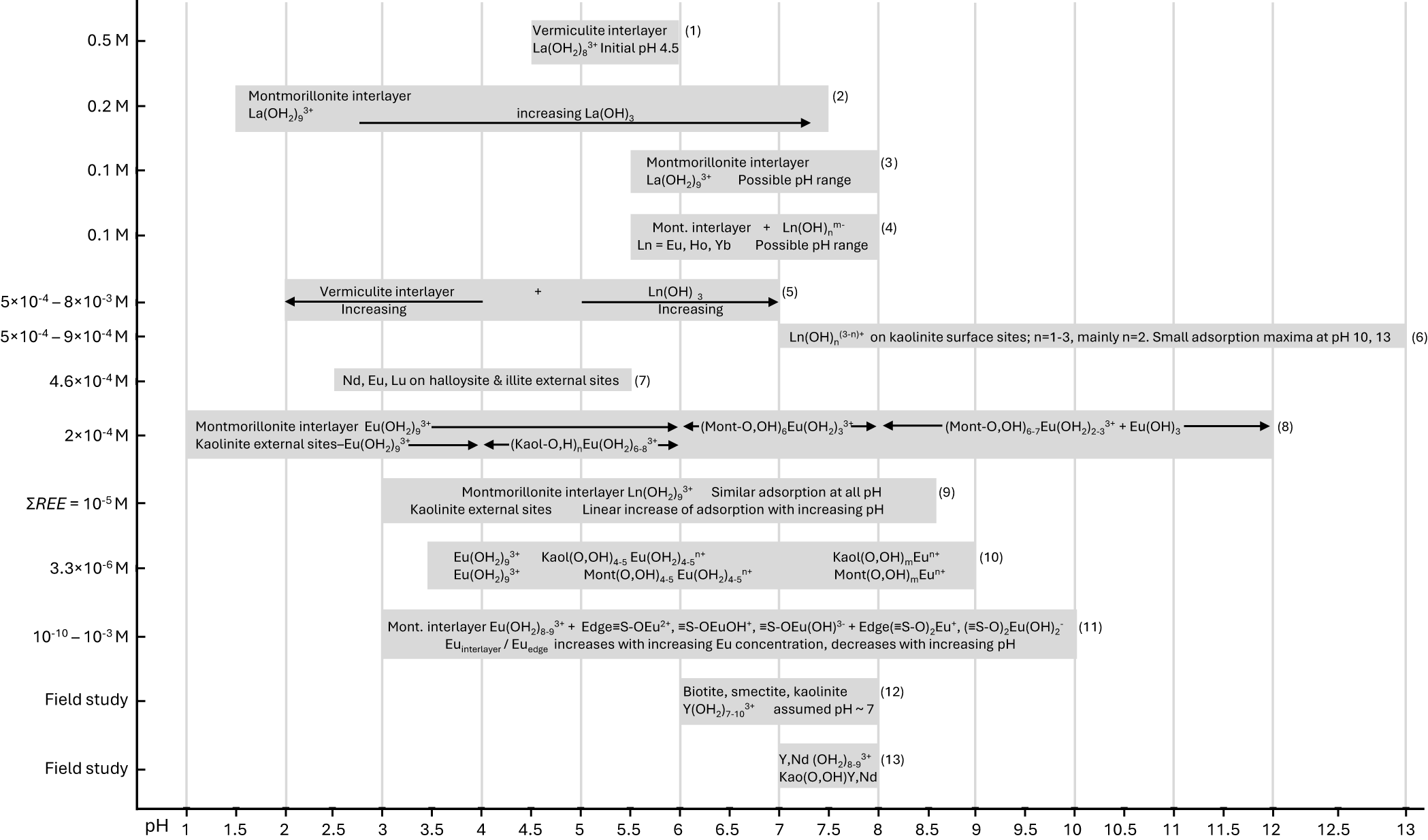

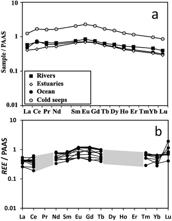


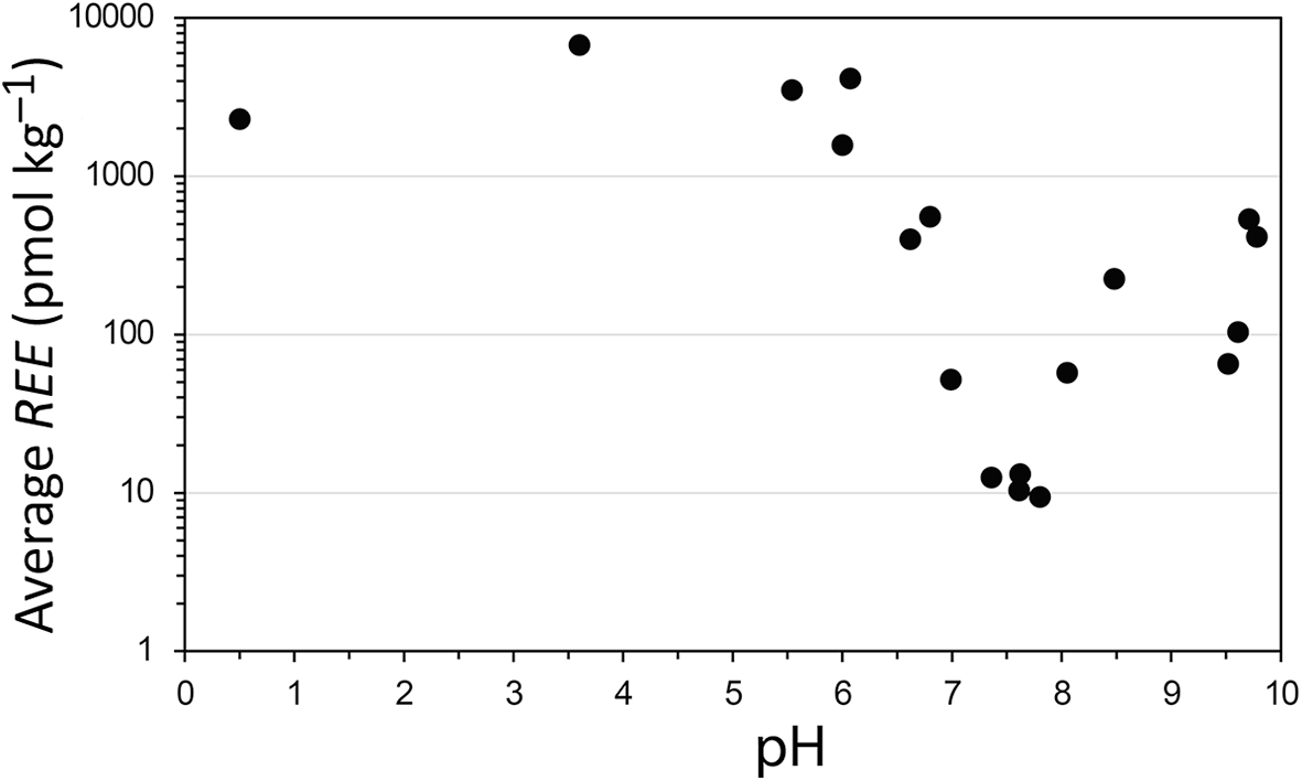


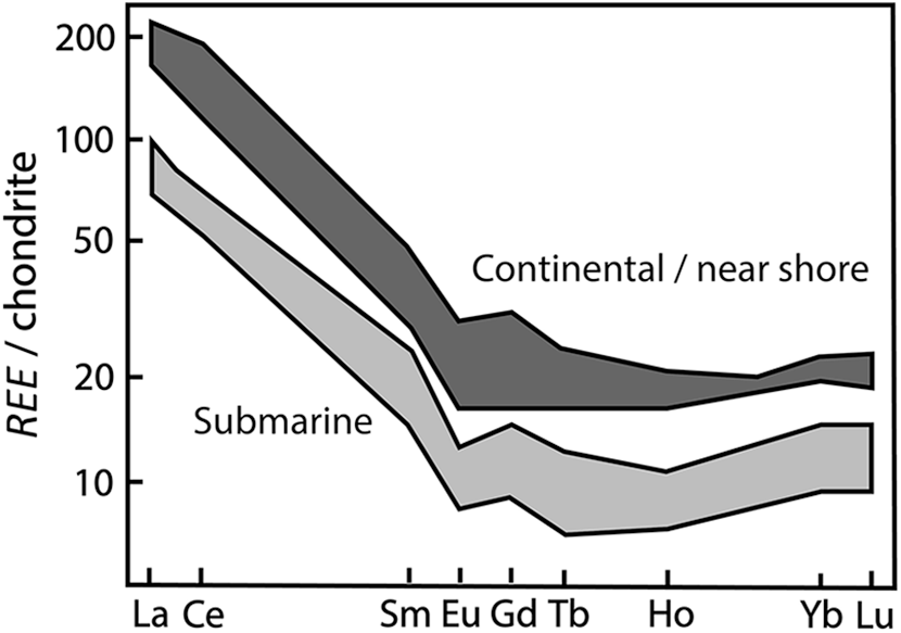

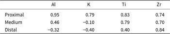


 Open access