


1 Introduction
Relationships among teachers are known to influence educational outcomes. Teachers’ relationships with each other are positively correlated with teaching performances (Spillane et al., Reference Spillane, Shirrell and Adhikari2018), perceptions of trust for peers (Kolleck et al., Reference Kolleck, Schuster, Hartmann and Gräsel2021) and students’ achievements, among others. In particular, teaching networks, composed of relationships in which teachers discuss their instructional practice with peers are vital to school climates. Teachers are more willing to engage with school policies if they feel more connected with other teachers and principals (Moolenaar et al., Reference Moolenaar, Daly and Sleegers2010). They are more willing to change and adopt new teaching practices if they are part of the teaching network and if the new practice has been adopted by teachers in their network (Penuel et al., Reference Penuel, Frank, Sun, Kim and Singleton2013). On the other hand, school climates are known to influence teaching networks. Teachers tend to have larger networks following professional development programs and tend to be more connected in schools that previously engaged in school-wide initiatives (Weinbaum et al., Reference Weinbaum, Cole, Weiss and Supovitz2008).
In this article, we study the relationship between teachers’ networks and school climates in schools. We study whether and how teachers’ advice interactions are related to their perceptions of schools. The network includes information about from whom the teachers seek advice during the school year. The school climates perceived by the teachers are measured as their responses to a set of survey questions called item responses.Footnote 1 Among the survey questions, three categories of questions were given to all teachers: perceived satisfaction with the school, perceived quality of the students, and perceived impact on school policies. To test and understand the relationship between the network and the perceived school climate, we propose a novel methodology that jointly analyzes a network and item responses from a questionnaire. Possible questions that can be answered with our methodology include whether the advice-seeking network or the latent dimensions of the advice-seeking network are related to the item responses or the latent dimensions of the item responses. Our methodology is applicable for the joint analysis of any data consisting of a network and item responses.
While several studies have looked into the relationship between the network of teachers and the school climate, rarely do they assess the relationship using fully specified statistical models (see, e.g., Broda et al., Reference Broda, Granger, Chow and Ross2023). More often, summary statistics are used as inputs for further assessment (Bonsignore et al., Reference Bonsignore, Hansen, Galyardt, Aleahmad and Hargadon2011), but focusing on summary statistics ignores important network information; in fact, two drastically different networks can be reduced to similar summary statistics, and thus the structures of the networks beyond the summary statistics are subsequently lost. For example, networks with similar node degree distributions can have different community structures (Paul & Chen, Reference Paul and Chen2022).
In this article, we develop a joint network and item response model (JNIRM), where we quantify and test the relationship between network and item responses via theorizing a shared data generation process for both data modalities. We devise the latent variables/spaces to describe the network formation (also called latent network dimensions) and the latent variables to describe the item responses, and quantify their co-varying dynamics with shared distributions. This approach allows the information in the item responses to inform the generation of the networks and has the potential to improve the cost efficiency of network studies without collecting information from new participants. Our proposed method offers new possibilities for investigations into the social factors of educational and health outcomes by increasing the amount of information utilized in estimating network parameters, leading to more powerful and cost-effective studies.
Compared with uni-modal models for only networks or item responses, our new method allows for more efficiently designed studies when the number of samples (cost of the conducting the proposed study) is constrained. Without collecting additional data with more study samples, our model is able to increase the precision of model parameter estimates and model predictive performances. This is because during our custom built Markov chain Monte Carlo (MCMC) estimation algorithm, the estimation of the latent network variables is not only informed by the network data, but also by the school climate item responses. In this way, we increase the amount of information in estimating network/item response parameters, leading to more powerful and cost-effective studies. In addition, modeling dependence as co-varying dynamics is a flexible and intuitive option. No prior knowledge about the direction of the dependence is needed.
The proposed method is different from that in Fosdick and Hoff (Reference Fosdick and Hoff2015), which models the correlation between latent variables estimated from a network and simple attribute data. Meanwhile, item responses or responses to questionnaires or test items are complicated types of attribute data with complex dimensionalities. A questionnaire consisting a multitude of survey items is often thoughtfully designed by domain expects (although AI-generated items recently became available) and is used to measure a specific facet of an individual, such as intelligence, personality trait, risk of developing psychiatric outcomes, or disordered behaviors and symptoms. Through this process, data from the item responses are used to indicate and differentiate individuals on abstract latent constructs. Not providing a latent variable theory about the generation of the item responses oversimplifies the problem and is a lost opportunity to model the measurement process. Thus, in such scenarios with multidimensional and dependent item responses, the method proposed in Fosdick and Hoff (Reference Fosdick and Hoff2015) may not be applicable.
In the following sections, we first describe the motivating application, followed by the JNIRM. We propose an MCMC algorithm to estimate the proposed model, and then we report results for the applications. Lastly, we discuss and conclude.
2 Motivating application
In this section, we present a real-life example, where the research question is whether and how a network and an item response matrix are related. School staff members in elementary schools were asked to list to whom they sought information and advice around mathematics instruction and curriculum. Data were collected in 2015 across $14$
elementary schools as part of a larger study in a mid-western school district in the United States (see more information about the data in the Supplementary Material).
$14$
elementary schools as part of a larger study in a mid-western school district in the United States (see more information about the data in the Supplementary Material).
We focus on one school from that district with 24 school staff members. Each staff member was asked to indicate to whom they turned for advice during the school year, and at most $12$
advisors were reported per teacher though all 24 listed less than
$12$
advisors were reported per teacher though all 24 listed less than $12$
. The presence of an at least monthly advice-seeking relationship is counted as an observed edge. In the adjacency matrix,
$12$
. The presence of an at least monthly advice-seeking relationship is counted as an observed edge. In the adjacency matrix, $x_{a,b}=1$
if teacher a seeks advice from teacher b. Because advice-seeking relationships are directional, and
$x_{a,b}=1$
if teacher a seeks advice from teacher b. Because advice-seeking relationships are directional, and $\boldsymbol {X}$
is asymmetric. Teacher a seeking advice from teacher b does not imply that teacher b seeks advice from teacher a. The degree distributions are shown in Figure 1. The indegree distribution is more skewed than the outdegree distribution suggesting that some of the advice was sought from a few experienced advisors, and not all individuals provided advice.
$\boldsymbol {X}$
is asymmetric. Teacher a seeking advice from teacher b does not imply that teacher b seeks advice from teacher a. The degree distributions are shown in Figure 1. The indegree distribution is more skewed than the outdegree distribution suggesting that some of the advice was sought from a few experienced advisors, and not all individuals provided advice.
Degree distribution for the advice-seeking network. Frequencies of number of persons one seeks advice from are outdegree, and frequencies of number of persons seeking advice from the same person are indegree.

Figure 2 shows the advice-seeking network where the staff members are shown as vertices and the arrows point from the advice-seeking to the advice provider. The number of arrows pointing to Node 1 indicates that Node 1 provided advice to many other staff members in that school. The density of this network is 0.14 meaning that 14% of the possible $24 \times 23$
advice-seeking relationships are observed. Reciprocity, the extent to which Node i asked Node j for advice also coincides with Node j asking Node i for advice, is 0.20 confirming that this network is largely asymmetric. Transitivity, the extent to which connections among pairs of nodes
$24 \times 23$
advice-seeking relationships are observed. Reciprocity, the extent to which Node i asked Node j for advice also coincides with Node j asking Node i for advice, is 0.20 confirming that this network is largely asymmetric. Transitivity, the extent to which connections among pairs of nodes $(i, j)$
and
$(i, j)$
and $(j, k)$
co-occurs with a connection between i and k, is 0.31. Transitivity is based on non-directional ties, so it is a better measure of how much school staff self-cluster in their networks. A transitivity of 0.31 indicates moderately low clustering.
$(j, k)$
co-occurs with a connection between i and k, is 0.31. Transitivity is based on non-directional ties, so it is a better measure of how much school staff self-cluster in their networks. A transitivity of 0.31 indicates moderately low clustering.
An advice-seeking social network among school staff in one school. Nodes are teachers, and the arrow points from the advice-seeker to the advice-provider.

Figure 2 Long description
At the center is node 1, which receives and sends multiple arrows to surrounding nodes, indicating it is a major advice provider and seeker. Nodes 2, 3, 10, 13, 16, 20, and 22 are densely connected to node 1, forming a core cluster. Arrows extend from node 1 to nodes 7, 12, 21, and 15, showing outward advice-seeking. Peripheral nodes such as 6, 9, 15, 18, and 24 have fewer connections, mostly receiving advice. Node 6 is isolated in the upper region, connected only through node 14. Node 19, 17, 5, 8, and 4 form a secondary cluster on the right, with arrows linking them to node 1 and each other. All arrows point from advice-seeker to advice-provider, mapping the directionality of advice flow. The network is asymmetric, with node 1 as the central hub and several peripheral nodes with limited connections.
The teachers were presented with the School Staff Social Network Questionnaire (SSSNQ; Pustejovsky & Spillane, Reference Pustejovsky and Spillane2009), which includes a variety of items about the school climate. We chose $16$
items on the questionnaire that were distributed to all teachers; of the
$16$
items on the questionnaire that were distributed to all teachers; of the $16$
items, four items are about the teacher’s overall satisfaction with the school (we will call these items the satisfaction items), seven items concern the teacher’s perceived influence over school policies (we will call these items the policy items), and five items concern the teacher’s perceptions of the students (we will call these items the student items). Each of the three subscales of the climate questionnaire includes items designed to measure a different construct: the satisfaction, the perceived influence over school policies, and the perception of students. We describe the complete list of questions under the three different constructs in the Supplementary Material.
$16$
items, four items are about the teacher’s overall satisfaction with the school (we will call these items the satisfaction items), seven items concern the teacher’s perceived influence over school policies (we will call these items the policy items), and five items concern the teacher’s perceptions of the students (we will call these items the student items). Each of the three subscales of the climate questionnaire includes items designed to measure a different construct: the satisfaction, the perceived influence over school policies, and the perception of students. We describe the complete list of questions under the three different constructs in the Supplementary Material.
The satisfaction items and the policy items were measured on a five-point Likert scale, and the student items were measured on a four-point scale. For the five-point scale, the response options were “Strongly Disagree,” “Disagree,” “Neutral,” “Agree,” and “Strongly Agree”; for the four-point scale, the response options were “None,” “A little,” “Some,” and “A great deal.” The scale data were treated as continuous using a linear model. We chose not to dichotomize the data because we found that after dichotomization, the data were not sufficiently informative for the latent structure of the items.
2.1 Dimensionality of the school climate questionnaire
We explored the dimensions of the item responses with a principle component analysis (PCA) of the correlation matrix. We applied the PCA to the data from all schools (see details of school-level dimensionality analysis in the Supplementary Material) to increase our sample size. Although a multigroup factor model or a multilevel factor model may be more appropriate, we considered a PCA as sufficient for an exploratory analysis, given that the inter-school differences were rather small (see the Supplementary Material for a comparison of four schools). The eigenvalues showed that there might be 3 or 4 components. The eigen values were $4.811 (28\%), 2.052 (14\%), 1.521 (9\%)$
, and
$4.811 (28\%), 2.052 (14\%), 1.521 (9\%)$
, and $1.060 (7\%)$
for the first four components, respectively.
$1.060 (7\%)$
for the first four components, respectively.
Given that there are three subscales in the questionnaire, we rotated the first three components to a theoretical target structure that corresponds to the three subscales (with a zero loading on the components that do not correspond to the subscale an item belongs to). All items of the same subscale were given the same high loadings in the target theoretical structure (i.e., a value of two different high values yield the same rotation result). The rotation was performed using Michael Browne’s target rotation, which is also implemented in CEFA (Browne et al., Reference Browne, Cudeck, Tateneni and Mels2008), using the target.rot function in the psych R package (Revelle & Revelle, Reference Revelle and Revelle2015).
The loadings of the rotated components are shown in Table 1. The loadings that are expected to be high based on the theoretical structure are in bold. The rotated components showed a clear correspondence with the theoretical structure, with the items from the same subscale loading on the same component and having low loadings on the other two components. To assess the similarity between the rotated components and the theoretical structure, we also calculated the congruence coefficients (see the results in Table 2). The congruence coefficients are the cosines between the rotated components and the components defined by the theoretical structure. Table 2 shows that the congruence coefficients are high between the corresponding components and the theoretical structure. Therefore, we believe that the three rotated components correspond to the three subscales. We will apply the same target rotation to the results from the joint analysis of the network data and questionnaire data in the application section. The joint model will be described next.
Rotated loadings of the PCA

Table 1 Long description
The table consists of 16 rows labeled Item 1 through Item 16 and three columns labeled Student, Policy, and Satisfaction. For each item, the corresponding loadings are listed. High loadings, as expected from the target matrix, are bolded. Item 1: Student 0.667, Policy 0.049, Satisfaction 0.091. Item 2: Student 0.731, Policy negative 0.003, Satisfaction 0.146. Item 3: Student 0.291, Policy negative 0.051, Satisfaction negative 0.062. Item 4: Student 0.563, Policy 0.076, Satisfaction 0.045. Item 5: Student 0.767, Policy negative 0.071, Satisfaction negative 0.158. Item 6: Student negative 0.054, Policy 0.591, Satisfaction 0.159. Item 7: Student 0.056, Policy 0.621, Satisfaction 0.014. Item 8: Student negative 0.018, Policy 0.881, Satisfaction negative 0.107. Item 9: Student negative 0.045, Policy 0.866, Satisfaction negative 0.155. Item 10: Student 0.032, Policy 0.736, Satisfaction negative 0.107. Item 11: Student 0.036, Policy 0.556, Satisfaction 0.164. Item 12: Student negative 0.007, Policy 0.630, Satisfaction 0.188. Item 13: Student 0.084, Policy 0.127, Satisfaction 0.671. Item 14: Student negative 0.132, Policy 0.034, Satisfaction 0.866. Item 15: Student negative 0.085, Policy negative 0.031, Satisfaction 0.922. Item 16: Student 0.183, Policy 0.001, Satisfaction 0.672. The note below the table states that high loadings expected from the target matrix are bolded.
Note: The loadings that are expected to be high based on the target matrix are in bold.
Congruence coefficients

Table 2 Long description
The table has four columns: Coefficients, Student, Policy, and Satisfaction. The first row lists the column headers. The first column lists the row headers: Student, Policy, Satisfaction. In the Student row, the values are 0.944 under Student, 0.000 under Policy, and 0.017 under Satisfaction. In the Policy row, the values are 0.000 under Student, 0.980 under Policy, and 0.035 under Satisfaction. In the Satisfaction row, the values are 0.017 under Student, 0.036 under Policy, and 0.953 under Satisfaction. Diagonal cells have the highest values, indicating strong self-congruence, while off-diagonal values are near zero.
3 The joint network and item response model
In this section, we describe the JNIRM. Conceptually, the model is a joint model for two kinds of data, and it consists of three components: (1) a model for the network data, (2) a model for the item response data, and (3) a joint component that connects the previous two components. We will explain each of the three components.
3.1 Modeling the network component
In a latent space model, a node’s information is summarized by low-dimensional continuous latent variables and can sometimes be visually represented in a low-dimensional space. The latent variable value for a node can be written in vector form with the number of elements in the vector equaling the number of dimensions. We restrict the scope of our discussion to vector latent space models that use the vector product to model the connections between nodes (see Wang, Reference Wang2021 for details about vector latent space models). One reason for using vector latent space models is to maintain consistency with the item response component of the joint framework. Models for item responses often use the vector product between a latent person variable and an item slope in the item response function, for example, the two-parameter IRT model and the factor models (De Boeck & Wilson, Reference De Boeck and Wilson2004).
We can summarize the relational information of person a as a sender in the network using a K-dimensional vector $\boldsymbol {u}_a$
, called the latent position of sender a. Similarly, we can summarize the relational information of person b as a receiver in the network using a K-dimensional vector
$\boldsymbol {u}_a$
, called the latent position of sender a. Similarly, we can summarize the relational information of person b as a receiver in the network using a K-dimensional vector $\boldsymbol {v}_b$
, called the latent position of receiver b. The latent position for a node is the coordinate of the node on the corresponding latent network dimension. In this article, we model the probability of a connection from a sender a to a receiver b using the vector product
$\boldsymbol {v}_b$
, called the latent position of receiver b. The latent position for a node is the coordinate of the node on the corresponding latent network dimension. In this article, we model the probability of a connection from a sender a to a receiver b using the vector product $\boldsymbol {u}_a^T\boldsymbol {v}_b$
, called the multiplicative UV effect. In network analysis, other forms of the vector products also exist, for example, the bilinear effect (Hoff, Reference Hoff2005). The multiplicative UV effects model allows for separate sender and receiver role specific latent variables for a node and is therefore more suitable for a directed network. For a directed network with a low level of reciprocity, the multiplicative UV effect is a better choice than the bilinear effect. We use the multiplicative UV effect to model the directed relationships in the advice-seeking network.
$\boldsymbol {u}_a^T\boldsymbol {v}_b$
, called the multiplicative UV effect. In network analysis, other forms of the vector products also exist, for example, the bilinear effect (Hoff, Reference Hoff2005). The multiplicative UV effects model allows for separate sender and receiver role specific latent variables for a node and is therefore more suitable for a directed network. For a directed network with a low level of reciprocity, the multiplicative UV effect is a better choice than the bilinear effect. We use the multiplicative UV effect to model the directed relationships in the advice-seeking network.
3.1.1 Continuous edge weights
We introduce the vector latent space model for a network with continuous quantitative edge weights. Let $\boldsymbol {X}$
be an
$\boldsymbol {X}$
be an $N \times N$
adjacency matrix representing the network, where N is the number of persons in the network. The edge value
$N \times N$
adjacency matrix representing the network, where N is the number of persons in the network. The edge value $X_{a,b}$
represents the relationship from sender a to receiver b,
$X_{a,b}$
represents the relationship from sender a to receiver b, $a,b =1,\ldots ,N$
and
$a,b =1,\ldots ,N$
and $b \neq a$
. For a directed network with continuous edge weights, the latent space model can be written as
$b \neq a$
. For a directed network with continuous edge weights, the latent space model can be written as

where $\delta $
is a fixed intercept parameter accounting for the density of the network. As mentioned before,
$\delta $
is a fixed intercept parameter accounting for the density of the network. As mentioned before, $\boldsymbol {u}_a$
and
$\boldsymbol {u}_a$
and $\boldsymbol {v}_b$
are latent positions for sender a and receiver b. The error for the edge from sender a to receiver b is
$\boldsymbol {v}_b$
are latent positions for sender a and receiver b. The error for the edge from sender a to receiver b is $e_{a,b}$
, and its covariance structure with
$e_{a,b}$
, and its covariance structure with $e_{b,a}$
follows Equation (3.1). We call
$e_{b,a}$
follows Equation (3.1). We call $\sigma ^2_e$
the error variance and
$\sigma ^2_e$
the error variance and $\rho $
the within-dyadFootnote
2
correlation. The within-dyad correlation accounts for reciprocity, that is, the degree to which relationships are reciprocated. When there is reciprocity,
$\rho $
the within-dyadFootnote
2
correlation. The within-dyad correlation accounts for reciprocity, that is, the degree to which relationships are reciprocated. When there is reciprocity, $X_{a,b}$
and
$X_{a,b}$
and $X_{b,a}$
are more likely to be the same. This model is identical to keeping only the multiplicative component of the additive and multiplicative effects (AME) model of Hoff (Reference Hoff2021). We use
$X_{b,a}$
are more likely to be the same. This model is identical to keeping only the multiplicative component of the additive and multiplicative effects (AME) model of Hoff (Reference Hoff2021). We use $\boldsymbol {U} $
and
$\boldsymbol {U} $
and $\boldsymbol {V} $
to denote the
$\boldsymbol {V} $
to denote the $N \times K$
matrices of the coordinates on the latent network dimensions for sender and receiver, and
$N \times K$
matrices of the coordinates on the latent network dimensions for sender and receiver, and $\boldsymbol {E}$
to denote the
$\boldsymbol {E}$
to denote the $N \times N$
matrix of network errors. The approximation of the posterior distributions of the unknown quantities is facilitated by setting prior distributions an
$N \times N$
matrix of network errors. The approximation of the posterior distributions of the unknown quantities is facilitated by setting prior distributions an $N(0, \sigma ^{-2}_0)$
with
$N(0, \sigma ^{-2}_0)$
with $\sigma ^{-2}_0>0$
for
$\sigma ^{-2}_0>0$
for $\delta $
, a
$\delta $
, a $\text {Unif}(-1, 1)$
for
$\text {Unif}(-1, 1)$
for $\rho $
, and a
$\rho $
, and a $\text {gamma} (1/2, 1/2)$
for
$\text {gamma} (1/2, 1/2)$
for $\sigma _e^{-2}$
. The prior for the covariance of the latent network dimensions is described in the joint component.
$\sigma _e^{-2}$
. The prior for the covariance of the latent network dimensions is described in the joint component.
Random node-specific intercepts or node specific additive effects can be added to the above network model (Hoff, Reference Hoff2021; Krivitsky et al., Reference Krivitsky, Handcock, Raftery and Hoff2009). In this case, Equation (3.1) will be modified to read $X_{a,b} = \delta + \eta _a + \xi _b + \boldsymbol {u}_a^T \boldsymbol {v}_b + e_{a,b}$
, with a suitable correlation structure on
$X_{a,b} = \delta + \eta _a + \xi _b + \boldsymbol {u}_a^T \boldsymbol {v}_b + e_{a,b}$
, with a suitable correlation structure on $\eta _a, \xi _b,\boldsymbol {u}_a$
, and
$\eta _a, \xi _b,\boldsymbol {u}_a$
, and $\boldsymbol {v}_b$
. Karrer and Newman (Reference Karrer and Newman2011) make a case for modeling the heterogeneity of the node degrees with additive node-level (fixed) effects in stochastic blockmodels, resulting in degree-corrected stochastic blockmodels (see discussions about the additive node-level effects in stochastic blockmodels in Jin, Reference Jin2015 and Zhao et al., Reference Zhao, Levina and Zhu2012). Without the additive node-level effects, blockmodels tend to identify clusters based on node degrees (e.g., a cluster of active nodes versus a cluster of less active nodes), especially when there is large heterogeneity in the node degrees. However, it is less clear if the additive node-level effects, for example, the random row and column intercepts
$\boldsymbol {v}_b$
. Karrer and Newman (Reference Karrer and Newman2011) make a case for modeling the heterogeneity of the node degrees with additive node-level (fixed) effects in stochastic blockmodels, resulting in degree-corrected stochastic blockmodels (see discussions about the additive node-level effects in stochastic blockmodels in Jin, Reference Jin2015 and Zhao et al., Reference Zhao, Levina and Zhu2012). Without the additive node-level effects, blockmodels tend to identify clusters based on node degrees (e.g., a cluster of active nodes versus a cluster of less active nodes), especially when there is large heterogeneity in the node degrees. However, it is less clear if the additive node-level effects, for example, the random row and column intercepts $\eta _a, \xi _b$
, are needed to model all types of networks in latent variable models. Indeed, the additive effects are useful to capture higher (or lower) nodal activity directed to all nodes in the network irrespective of their positions in the latent space. On the other hand, the length of the latent variable of the node contributes to the activity level of the node in relation to other nodes in the space—this is captured by the multiplicative nature of the vector products to model connections. In small data sets with moderate levels of heterogeneity of the node degrees, the latent positions alone might be sufficient for modeling the activity levels of the nodes. Although, in principle, we can expect improvement in the recovery of the node degrees with added additive effects, a situation might arise where the improvement is negligible.
$\eta _a, \xi _b$
, are needed to model all types of networks in latent variable models. Indeed, the additive effects are useful to capture higher (or lower) nodal activity directed to all nodes in the network irrespective of their positions in the latent space. On the other hand, the length of the latent variable of the node contributes to the activity level of the node in relation to other nodes in the space—this is captured by the multiplicative nature of the vector products to model connections. In small data sets with moderate levels of heterogeneity of the node degrees, the latent positions alone might be sufficient for modeling the activity levels of the nodes. Although, in principle, we can expect improvement in the recovery of the node degrees with added additive effects, a situation might arise where the improvement is negligible.
In this article, we choose not to include additive effects in the network component of the framework. In our application of the advice-seeking network and the school climate questionnaire, we observe comparable recovery of node degrees as well as comparable model fit with and without the nodal effects in the model. Therefore, we think the nodal effects are not needed in the modeling of the advice-seeking network though this might not be the case for other networks.
Although the proposed approach for the network component of the joint framework can be seen as an AME model, the difference of our approach is that we connect the network component with the item response component using a covariance-based joint component. See details about the joint component in Section 3.3.
3.1.2 Identifiability
The coordinates of the latent network dimensions, $\boldsymbol {U}$
and
$\boldsymbol {U}$
and $\boldsymbol {V,}$
are identified up to rotations, while
$\boldsymbol {V,}$
are identified up to rotations, while $\boldsymbol {U}\boldsymbol {V}^T$
is directly identified following the condition that either
$\boldsymbol {U}\boldsymbol {V}^T$
is directly identified following the condition that either $\boldsymbol {U}$
or
$\boldsymbol {U}$
or $\boldsymbol {V}$
is centered. Suppose
$\boldsymbol {V}$
is centered. Suppose $\boldsymbol {1}_N$
is the N-dimensional column vector of
$\boldsymbol {1}_N$
is the N-dimensional column vector of $1$
s;
$1$
s; $\boldsymbol {J}_N = \boldsymbol {1}_N \boldsymbol {1}_N^T$
is the
$\boldsymbol {J}_N = \boldsymbol {1}_N \boldsymbol {1}_N^T$
is the $N \times N$
matrix of
$N \times N$
matrix of $1$
s; and
$1$
s; and $\boldsymbol {H}$
is the centering matrix,
$\boldsymbol {H}$
is the centering matrix, $\boldsymbol {H} = \boldsymbol {I}_N - \frac {1}{N} \boldsymbol {1}_N \boldsymbol {1}_N^T$
.
$\boldsymbol {H} = \boldsymbol {I}_N - \frac {1}{N} \boldsymbol {1}_N \boldsymbol {1}_N^T$
.
Lemma 1. Let either $\boldsymbol {U}$
or
$\boldsymbol {U}$
or $\boldsymbol {V}$
be centered, that is,
$\boldsymbol {V}$
be centered, that is, $ \boldsymbol {H}\boldsymbol {U} = \boldsymbol {U}\text {or } \boldsymbol {H}\boldsymbol {V} = \boldsymbol {V}$
. If two sets of parameters
$ \boldsymbol {H}\boldsymbol {U} = \boldsymbol {U}\text {or } \boldsymbol {H}\boldsymbol {V} = \boldsymbol {V}$
. If two sets of parameters $\delta $
,
$\delta $
, $\boldsymbol {U} $
,
$\boldsymbol {U} $
, $\boldsymbol {V} $
, and
$\boldsymbol {V} $
, and $\delta '$
,
$\delta '$
, $\boldsymbol {U'} $
,
$\boldsymbol {U'} $
, $\boldsymbol {V'} $
lead to the same
$\boldsymbol {V'} $
lead to the same $E(X_{a,b})$
, then
$E(X_{a,b})$
, then $\delta = \delta '$
,
$\delta = \delta '$
, $\boldsymbol {U} = \boldsymbol {U'} \boldsymbol {O} $
, and
$\boldsymbol {U} = \boldsymbol {U'} \boldsymbol {O} $
, and $\boldsymbol {V} = \boldsymbol {V'} \boldsymbol {O}^{-1} $
, where
$\boldsymbol {V} = \boldsymbol {V'} \boldsymbol {O}^{-1} $
, where $\boldsymbol {O}$
is a
$\boldsymbol {O}$
is a $K \times K$
nonsingular matrix.
$K \times K$
nonsingular matrix.
The proof of this lemma is in the Supplementary Material. The proof follows similar arguments to those laid out in Huang et al. (Reference Huang, Soliman, Paul and Xu2022) and Zhang et al. (Reference Zhang, Xue and Zhu2020). To resolve the rotational indeterminacy and reflection of the axes in the latent space, we follow the approach in Fosdick and Hoff (Reference Fosdick and Hoff2015), Hoff (Reference Hoff2015a, Reference Hoff2021), and Minhas et al. (Reference Minhas, Hoff and Ward2019) and use the first K left and right singular vectors of the posterior means of the vector products as the estimates of $\boldsymbol {U}$
and
$\boldsymbol {U}$
and $\boldsymbol {V}$
. In this way, we can obtain estimates of the latent positions following the convergence of the vector products, and not the convergence of the latent positions themselves. The convergence of the vector products will be assessed and reported. The consequence of this approach is that we do not have a posterior distribution of the latent positions, only of the vector products.
$\boldsymbol {V}$
. In this way, we can obtain estimates of the latent positions following the convergence of the vector products, and not the convergence of the latent positions themselves. The convergence of the vector products will be assessed and reported. The consequence of this approach is that we do not have a posterior distribution of the latent positions, only of the vector products.
3.1.3 Binary network
The observed advice-seeking network in our application is binary and not continuous. We model the observed binary edge $X_{a,b}$
as the binary indicator that the latent continuous measure,
$X_{a,b}$
as the binary indicator that the latent continuous measure, $\phi _{a,b}$
is bigger than zero, that is,
$\phi _{a,b}$
is bigger than zero, that is, $X_{a,b} = 1$
, when
$X_{a,b} = 1$
, when $\phi _{a,b}>0$
. For a binary network,
$\phi _{a,b}>0$
. For a binary network, $\phi _{a,b}$
replaces
$\phi _{a,b}$
replaces $X_{a,b}$
in the proposed methodology in Equation (3.1). The error variance of the latent continuous measure is assumed to be
$X_{a,b}$
in the proposed methodology in Equation (3.1). The error variance of the latent continuous measure is assumed to be $1$
(as in probit models) to identify the scale of the latent continuous measure.
$1$
(as in probit models) to identify the scale of the latent continuous measure.
3.2 Modeling the item response component
To model the school climate questionnaire, we propose a latent variable model with vector products for continuous observations. Through this methodology, we aim to get three sets of information: (1) item intercept, (2) item slope, and (3) the latent variable values. The item intercept reflects the average of the responses across all persons for each item. A higher intercept indicates a higher average response. The item slope reflects how well the item differentiates in terms of the latent variable. One unit difference in the latent variable results in a large difference in the probabilities of response when the item slope is large.
Consider the continuous item responses, $\boldsymbol {Y}$
, an
$\boldsymbol {Y}$
, an $N \times M$
matrix, where N is the number of persons and M is the number of items. The response,
$N \times M$
matrix, where N is the number of persons and M is the number of items. The response, $Y_{p,i}$
, represents person p’s response to item i,
$Y_{p,i}$
, represents person p’s response to item i, $p = 1,2,\ldots , N$
and
$p = 1,2,\ldots , N$
and $i = 1,2,\ldots , M$
. Let D be the number of dimensions or latent variables in the item responses. The model can be written as
$i = 1,2,\ldots , M$
. Let D be the number of dimensions or latent variables in the item responses. The model can be written as
 $$ \begin{align} Y_{p,i} = \beta_i + \boldsymbol{\alpha}_i^T \boldsymbol{\theta}_p + \epsilon_{p,i}, \qquad \boldsymbol{\theta}_p \overset{iid}{\sim} \text{MVN}(0, \Lambda_{\theta}) , \qquad \epsilon_{p,i} \overset{iid}{\sim} N(0, \sigma^2_{\epsilon}), \end{align} $$
where $\boldsymbol {\alpha }_i$
and
$\boldsymbol {\alpha }_i$
and $\boldsymbol {\theta }_p$
are the D-dimensional vectors containing the item slopes and the person latent variables of the item responses;
$\boldsymbol {\theta }_p$
are the D-dimensional vectors containing the item slopes and the person latent variables of the item responses; $\beta _i$
is the intercept of item i; and
$\beta _i$
is the intercept of item i; and $\sigma ^2_{\epsilon }$
is the error variance for the item responses. As is common in models for item responses, the parameters for the items (including the item slope,
$\sigma ^2_{\epsilon }$
is the error variance for the item responses. As is common in models for item responses, the parameters for the items (including the item slope, $\boldsymbol {\alpha }_i$
and the item intercept,
$\boldsymbol {\alpha }_i$
and the item intercept, $\beta _i$
) are fixed, and the person variable,
$\beta _i$
) are fixed, and the person variable, $\boldsymbol {\theta }_p$
are random. We use
$\boldsymbol {\theta }_p$
are random. We use $\boldsymbol {\beta } $
to denote the
$\boldsymbol {\beta } $
to denote the $M \times 1$
vector of item intercepts,
$M \times 1$
vector of item intercepts, $\boldsymbol {A}$
to denote the
$\boldsymbol {A}$
to denote the $M \times D$
matrix of item slopes,
$M \times D$
matrix of item slopes, $\boldsymbol {\Theta }$
to denote the
$\boldsymbol {\Theta }$
to denote the $N \times D$
matrix of latent variables of item responses, and
$N \times D$
matrix of latent variables of item responses, and $\boldsymbol {\Psi }$
to denote the
$\boldsymbol {\Psi }$
to denote the $N \times M$
matrix of item response errors. Let us define
$N \times M$
matrix of item response errors. Let us define $\boldsymbol {\xi }_i$
as a vector of item parameters,
$\boldsymbol {\xi }_i$
as a vector of item parameters, $ \boldsymbol {\xi }_i = (\boldsymbol {\alpha }_i^T, \beta _i)^T$
. Approximation of the posterior distribution of the item parameters is facilitated by setting a
$ \boldsymbol {\xi }_i = (\boldsymbol {\alpha }_i^T, \beta _i)^T$
. Approximation of the posterior distribution of the item parameters is facilitated by setting a $\text {MVN} (\boldsymbol {\mu }_{\xi }, \boldsymbol {\Sigma }_{\xi }), \boldsymbol {\mu }_{\xi } = (1,1,\ldots ,1,0)^T, \boldsymbol {\Sigma }_{\xi } = \boldsymbol {I}_{D+1} $
prior distribution for
$\text {MVN} (\boldsymbol {\mu }_{\xi }, \boldsymbol {\Sigma }_{\xi }), \boldsymbol {\mu }_{\xi } = (1,1,\ldots ,1,0)^T, \boldsymbol {\Sigma }_{\xi } = \boldsymbol {I}_{D+1} $
prior distribution for $\boldsymbol {\xi }_i$
. We set a prior distribution of
$\boldsymbol {\xi }_i$
. We set a prior distribution of $\text {gamma } (1/2, 1/2)$
for
$\text {gamma } (1/2, 1/2)$
for $\sigma _{\epsilon }^{-2}$
. The prior for the covariance of the latent variables of the item responses is described in the joint component. In the case of binary item response, similar to binary network edge value, we can model the binary network response as the binary indicator that the latent continuous measure,
$\sigma _{\epsilon }^{-2}$
. The prior for the covariance of the latent variables of the item responses is described in the joint component. In the case of binary item response, similar to binary network edge value, we can model the binary network response as the binary indicator that the latent continuous measure, $\eta _{p,i}$
is larger than zero, that is,
$\eta _{p,i}$
is larger than zero, that is, $Y_{p,i} = 1$
, when
$Y_{p,i} = 1$
, when $\eta _{p,i}>0$
.
$\eta _{p,i}>0$
.
Identifiability: The latent variables of the item responses and the item slopes, $\boldsymbol {\Theta }$
and
$\boldsymbol {\Theta }$
and $\boldsymbol {A,}$
are identified up to rotations while
$\boldsymbol {A,}$
are identified up to rotations while $\boldsymbol {\Theta } \boldsymbol {A}^T$
is directly identified following the condition that either
$\boldsymbol {\Theta } \boldsymbol {A}^T$
is directly identified following the condition that either $\boldsymbol {\Theta }$
or
$\boldsymbol {\Theta }$
or $\boldsymbol {A}$
is centered. Following convention, we focus on the condition that
$\boldsymbol {A}$
is centered. Following convention, we focus on the condition that $\boldsymbol {\Theta }$
is centered.
$\boldsymbol {\Theta }$
is centered.
Lemma 2. Assume $\boldsymbol {\Theta }$
is centered, that is,
$\boldsymbol {\Theta }$
is centered, that is, $ \boldsymbol {H}\boldsymbol {\Theta } = \boldsymbol {\Theta }$
. If two sets of parameters
$ \boldsymbol {H}\boldsymbol {\Theta } = \boldsymbol {\Theta }$
. If two sets of parameters $\boldsymbol {\beta }$
,
$\boldsymbol {\beta }$
, $\boldsymbol {\Theta } $
,
$\boldsymbol {\Theta } $
, $\boldsymbol {A} $
, and
$\boldsymbol {A} $
, and $\boldsymbol {\beta '}$
,
$\boldsymbol {\beta '}$
, $\boldsymbol {\Theta }' $
,
$\boldsymbol {\Theta }' $
, $\boldsymbol {A}' $
lead to the same
$\boldsymbol {A}' $
lead to the same $E(Y_{p,i})$
, then
$E(Y_{p,i})$
, then $\boldsymbol {\beta } = \boldsymbol {\beta '}$
,
$\boldsymbol {\beta } = \boldsymbol {\beta '}$
, $\boldsymbol {\Theta } = \boldsymbol {\Theta '} \boldsymbol {O} $
, and
$\boldsymbol {\Theta } = \boldsymbol {\Theta '} \boldsymbol {O} $
, and $\boldsymbol {A} = \boldsymbol {A'} \boldsymbol {O}^{-1} $
, where
$\boldsymbol {A} = \boldsymbol {A'} \boldsymbol {O}^{-1} $
, where $\boldsymbol {O}$
is a
$\boldsymbol {O}$
is a $D \times D$
nonsingular matrix.
$D \times D$
nonsingular matrix.
The proof of Lemma 2 is in the Supplementary Material. In addition to the condition identified above, we also fix the latent variables to have unit variances and orthogonality between dimensions following the current factor model (and item response model) literature. Similar to the network component of the JNIRM, we also use the first D left and right singular vectors of the posterior means of the vector products as the estimates of $\boldsymbol {\theta }$
and
$\boldsymbol {\theta }$
and $\boldsymbol {\alpha }$
. In this approach, only the convergence of the vector products is needed for the estimation of the item slopes and the person variables, not the convergence of the item slopes and the latent variables themselves.
$\boldsymbol {\alpha }$
. In this approach, only the convergence of the vector products is needed for the estimation of the item slopes and the person variables, not the convergence of the item slopes and the latent variables themselves.
3.3 Modeling the joint component
Recall that the network component of the joint framework is modeled following Equation (3.1), and that the item response component of the joint framework is modeled following Equation (3.2). In these two components, we use normal distributions for the network dimensions and the latent variables of the item responses separately. To connect these two sets of variables, we use a multivariate normal distribution with a joint covariance matrix:

In Equation (3.3), we use $\boldsymbol {\Sigma }_{u\theta }$
to denote the omnibus covariance matrix capturing the co-varying relationships between network and item responses, which can be partitioned into four blocks,
$\boldsymbol {\Sigma }_{u\theta }$
to denote the omnibus covariance matrix capturing the co-varying relationships between network and item responses, which can be partitioned into four blocks, $\Lambda _u$
,
$\Lambda _u$
, $\Lambda _{u\theta }^T$
,
$\Lambda _{u\theta }^T$
, $\Lambda _{u\theta }$
, and
$\Lambda _{u\theta }$
, and $\Lambda _{\theta }$
with
$\Lambda _{\theta }$
with $\Lambda _{u\theta }^T$
being the transpose of
$\Lambda _{u\theta }^T$
being the transpose of $\Lambda _{u\theta }$
containing the same parameters. In this notation, for simplicity and to reduce the complexity of notations, we use subscript u to denote the network component, omitting subscript v, and subscript
$\Lambda _{u\theta }$
containing the same parameters. In this notation, for simplicity and to reduce the complexity of notations, we use subscript u to denote the network component, omitting subscript v, and subscript $\theta $
to denote the item response component. Approximation of the posterior distribution of
$\theta $
to denote the item response component. Approximation of the posterior distribution of $ \boldsymbol {\Sigma }_{u\theta } $
is facilitated by setting a prior distribution of
$ \boldsymbol {\Sigma }_{u\theta } $
is facilitated by setting a prior distribution of $ \text {Wishart} (\boldsymbol {I}_{2K+D}, 2K+D+2)$
. The covariance of the latent network dimensions
$ \text {Wishart} (\boldsymbol {I}_{2K+D}, 2K+D+2)$
. The covariance of the latent network dimensions $(\boldsymbol {u}_p, \boldsymbol {v}_p)^T$
is the
$(\boldsymbol {u}_p, \boldsymbol {v}_p)^T$
is the $2K \times 2K$
matrix
$2K \times 2K$
matrix $\boldsymbol {\Lambda }_{u}$
, and the covariance of the latent variables of the item responses is the
$\boldsymbol {\Lambda }_{u}$
, and the covariance of the latent variables of the item responses is the $D \times D$
matrix
$D \times D$
matrix $\boldsymbol {\Lambda }_{\theta }$
. If the network dimensions are independent, then
$\boldsymbol {\Lambda }_{\theta }$
. If the network dimensions are independent, then $\boldsymbol {\Lambda }_{u}$
is a diagonal matrix. If the dimensions of the item responses are independent, then
$\boldsymbol {\Lambda }_{u}$
is a diagonal matrix. If the dimensions of the item responses are independent, then $\boldsymbol {\Lambda }_{\theta }$
is a diagonal matrix. In JNIRM, we can test whether the network and item responses are dependent by testing whether the
$\boldsymbol {\Lambda }_{\theta }$
is a diagonal matrix. In JNIRM, we can test whether the network and item responses are dependent by testing whether the $D \times 2K$
matrix
$D \times 2K$
matrix $\boldsymbol {\Lambda }_{u\theta } = 0.$
See details in the next section. The model is estimated using a Gibbs sampler outlined in Section 4.
$\boldsymbol {\Lambda }_{u\theta } = 0.$
See details in the next section. The model is estimated using a Gibbs sampler outlined in Section 4.
3.4 Advantages
The superiority of JNIRM includes (1) more realistic model representation of the mutual impact of social relationship and school climate, (2) flexible accommodations of missing observations, and (3) cost effective study designs that improve precision of inference without collecting additional data. First, unlike regression models that assume one-directional relationships between advice-seeking networks and three school climate dimensions,—assuming that school climate dimensions impact teachers’ advice-seeking behaviors or vice versa—JNIRM acknowledges the mutual relationship between them. Changes in the school climate often correlate with changes in advice-seeking networks, but teachers’ relationships with each other can also influence school climate. In this way, JNIRM can offer a more realistic representation of the relationship between the advice-seeking networks and school climate, allowing for a more flexible interpretation of the results. Second, network regression models with school climate as covariates assume that each teacher’s school climate score is available (covariates are assumed to be fixed observations in a regression model) and that the school climate data are fully observed (no missing observation can be accommodated in covariates of a regression model). This assumption becomes problematic when data include missing observations for teacher’s school climate scores; in such situations, these teachers’ information may be discarded from the model, or additional data processing procedures for missing data are warranted, which often comes with their own modeling assumptions and inconsistencies. Regression methods struggle to handle situations where data are incomplete when incorporating school climate information as covariates. Lastly, by simultaneously modeling the reciprocal influence between networks and behaviors in a shared data generation process, we are able to improve model performance and prediction accuracy in certain situations where networks are sparse. During the MCMC sampling, the estimation of the latent network variables is not only informed by the network data, but also by the school climate item responses. In this way, without collecting additional data with more sample size, we are able to increase the amount of information in estimating network parameters, leading to more powerful and cost-effective studies.
3.5 Exploring the dependence between the network and item responses
In this section, we discuss how to make inferences regarding the dependence between the network and item responses. Due to the previously described solution for the identification issues, we cannot directly determine uncertainty about the covariance matrix based on the MCMC chain. Instead, following Fosdick and Hoff (Reference Fosdick and Hoff2015), we use the multivariate test of independence and the CCA to study the dependence between the two components of the joint framework. We first discuss the test and then CCA.
3.5.1 The multivariate test of independence
The classical multivariate test of independence (see Anderson, Reference Anderson1962) is applied using the estimated network dimensions and the latent variables of the item response. More specifically, the null and the alternative hypotheses of the test are
 $$ \begin{align} H_0: \Lambda_{u\theta} = 0 \qquad \text{vs.} \qquad H_1: \Lambda_{u\theta} \neq 0. \end{align} $$
The test statisticFootnote
3
is $t = \frac {\max _{ \Lambda _u, \Lambda _{\theta }} L_0(\Lambda _u, \Lambda _{\theta } | \boldsymbol {u}_p, \boldsymbol {v}_p, \boldsymbol {\theta }_p) }{ \max _{\boldsymbol {\Sigma }_{u\theta }} L(\boldsymbol {\Sigma }_{u\theta }|\boldsymbol {u}_p, \boldsymbol {v}_p, \boldsymbol {\theta }_p)} = \left ( \frac { |\hat {\boldsymbol {\Sigma }}_{u\theta }|}{|\hat {\Lambda }_u| \cdot | \hat {\Lambda }_{\theta }|} \right )$
, where
$t = \frac {\max _{ \Lambda _u, \Lambda _{\theta }} L_0(\Lambda _u, \Lambda _{\theta } | \boldsymbol {u}_p, \boldsymbol {v}_p, \boldsymbol {\theta }_p) }{ \max _{\boldsymbol {\Sigma }_{u\theta }} L(\boldsymbol {\Sigma }_{u\theta }|\boldsymbol {u}_p, \boldsymbol {v}_p, \boldsymbol {\theta }_p)} = \left ( \frac { |\hat {\boldsymbol {\Sigma }}_{u\theta }|}{|\hat {\Lambda }_u| \cdot | \hat {\Lambda }_{\theta }|} \right )$
, where $L_0$
and L are the likelihood with and without restricting
$L_0$
and L are the likelihood with and without restricting $\Lambda _{u\theta }=0$
, and estimates of the covariance matrix are obtained using the estimated latent network dimensions and the latent variables of the item responses. The critical region of the test is
$\Lambda _{u\theta }=0$
, and estimates of the covariance matrix are obtained using the estimated latent network dimensions and the latent variables of the item responses. The critical region of the test is $t < t(\alpha )$
, where
$t < t(\alpha )$
, where $t(\alpha )$
is the threshold value such that the probability of an observed t is smaller than
$t(\alpha )$
is the threshold value such that the probability of an observed t is smaller than $t(\alpha )$
with probability
$t(\alpha )$
with probability $\alpha $
.
$\alpha $
.
3.5.2 Canonical correlation analysis
Following the rejection of the null hypothesis in the classical multivariate test of independence between the network and item responses, we may wish to know where the lack of independence lies. We can use the CCA to achieve this goal. In this section, we provide a brief overview of CCA, and we focus on how it can be applied to understand the relationship between the network and item responses. For more detailed discussions about this topic, we refer readers to Anderson (Reference Anderson1962), Marden (Reference Marden2015), Sherry and Henson (Reference Sherry and Henson2005), and Thorndike (Reference Thorndike2000).
CCA is a useful technique to study the relationship between two sets of variables. In this case, the first set of variables includes the network dimensions from the network component of the JNIRM, and the second set of variables includes the latent variables from the item response component of the JNIRM. Using CCA, we estimate the largest correlation obtainable between a linear combination of the network dimensions and a linear combination of the latent variables of the item responses. Then, a second largest correlation is obtained with linear combinations that are uncorrelated with the first linear combinations. The process is repeated, with each set of linear combinations maximizing the correlation subject to being uncorrelated with the previous combinations.
In Figure 3, we demonstrate CCA with a hypothetical JNIRM when the number of dimensions for the network is two, and the number of dimensions for the item responses is three. In the left side of the figure, the latent variables of the item responses are linearly combined to create the item response canonical function, and a similar process occurs in the right side of the figure for the network. The weights of the linear combination are called the canonical weights or the function coefficients, and the resulting weighted sum is called the canonical function. For example, an item response canonical function is the weighted sum of the latent variables of the item responses. There can be as many canonical functions as the smallest set of variables at one of the two sides. The canonical functions are orthogonal to each other following the independence of the linear combinations. We will base our interpretations with CCA on standardized function coefficients.
Illustration of the network and item response canonical functions in a canonical correlation analysis with three latent variables from the item responses and two network dimensions. The canonical correlation is the correlation between the network and item response canonical functions, which are linear combinations of the item response latent variables and the network dimensions.

Figure 3 Long description
On the left, three stacked rectangles labeled item response latent variable 1, item response latent variable 2, and item response latent variable 3 each have arrows pointing right to an oval labeled item response canonical function. This oval is connected by a double-headed arrow labeled canonical correlation R to a second oval labeled network canonical function. From this second oval, four arrows extend rightward to four stacked rectangles labeled network sender dimension 1, network sender dimension 2, network receiver dimension 1, and network receiver dimension 2. The diagram illustrates the mapping of three item response latent variables into a canonical function, which is then correlated with a network canonical function composed of two sender and two receiver dimensions.
In the center of Figure 3, the canonical correlation, $R,$
is shown as the correlation between the network and the item response canonical functions. The square of the canonical correlation,
$R,$
is shown as the correlation between the network and the item response canonical functions. The square of the canonical correlation, $R^2$
, represents the proportion of variance shared by the network and the item response canonical functions. The square of the second canonical correlation indicates the proportion of the shared variance between the second pair of canonical functions based on the remaining relationship (independent of the first pair of canonical functions).
$R^2$
, represents the proportion of variance shared by the network and the item response canonical functions. The square of the second canonical correlation indicates the proportion of the shared variance between the second pair of canonical functions based on the remaining relationship (independent of the first pair of canonical functions).
Significance tests can be conducted in association with the canonical correlations. Testing each correlation separately for statistical significance is not readily available, instead, the correlations are tested in a hierarchal fashion. First, we test whether all correlations are zero; if that null hypothesis is rejected, we can test whether the $I-1$
(I is the total number of canonical correlations) smallest correlations are—or whether the remaining shared variance is—zero, etc.
$I-1$
(I is the total number of canonical correlations) smallest correlations are—or whether the remaining shared variance is—zero, etc.
4 Bayesian inference
In this section, we propose an algorithm for estimating the proposed JNIRM using MCMC methods. We devise a Gibbs sampler for the proposed model and discuss how to model binary data. In the following, we provide details of the full conditionals for each unknown quantity, and the algorithm is implemented through iterative sampling of the unknown quantities from their full conditional distributions. With sufficient iterations, we obtain stable Markov chains to approximate various quantities of the targeted posterior distributions. With random initial values on the unknown parameters, we conduct posterior computation by iterating the following steps:
-
• simulate $\boldsymbol {U}, \boldsymbol {V}$
from their full conditional distributions;
$\boldsymbol {U}, \boldsymbol {V}$
from their full conditional distributions; -
• simulate
$\boldsymbol {\Theta }$
from their full conditional distributions; -
• simulate
$\boldsymbol {\Sigma }_{u \theta }$
from its full conditional distribution; -
• simulate
$\sigma ^{-2}_e$
,
$\rho ,$
and
$\delta $
from their full conditional distributions; -
• simulate
$\sigma ^{-2}_{\epsilon }$
from its full conditional distributions; -
• simulate
$\boldsymbol {\xi }_i$
from its full conditional distributions.


4.1 Full conditionals of the latent variables and the covariance
4.1.1 Multiplicative UV effect
The item responses are related to the network through the dependence between $\boldsymbol {\Theta }$
and
$\boldsymbol {\Theta }$
and $\boldsymbol {U}, \boldsymbol {V}$
. We are interested in the joint full conditional distribution of
$\boldsymbol {U}, \boldsymbol {V}$
. We are interested in the joint full conditional distribution of $\boldsymbol {\Theta }$
and
$\boldsymbol {\Theta }$
and $\boldsymbol {U}, \boldsymbol {V}$
. For person p, we focus on the first dimension for sender,
$\boldsymbol {U}, \boldsymbol {V}$
. For person p, we focus on the first dimension for sender, $u_{p,1}$
conditional on the other dimensions,
$u_{p,1}$
conditional on the other dimensions, $u_{p,2},\ldots ,u_{p,K}$
and all dimensions of
$u_{p,2},\ldots ,u_{p,K}$
and all dimensions of $\boldsymbol {v}_p $
,
$\boldsymbol {v}_p $
, $\boldsymbol {v}_p = (v_{p,1},\ldots ,v_{p,K})^T$
. Given that
$\boldsymbol {v}_p = (v_{p,1},\ldots ,v_{p,K})^T$
. Given that $\boldsymbol {u}_p, \boldsymbol {v}_p$
, and
$\boldsymbol {u}_p, \boldsymbol {v}_p$
, and $\boldsymbol {\theta }_p$
follow a multivariate normal distribution, the joint probability model for
$\boldsymbol {\theta }_p$
follow a multivariate normal distribution, the joint probability model for $u_{p,1}$
and
$u_{p,1}$
and $\theta _{p,1}$
,…,
$\theta _{p,1}$
,…, $\theta _{p,D}$
conditional on
$\theta _{p,D}$
conditional on $u_{p,2},\ldots ,u_{p,K}$
and
$u_{p,2},\ldots ,u_{p,K}$
and $\boldsymbol {v}_p$
is also a multivariate normal distribution with conditional mean
$\boldsymbol {v}_p$
is also a multivariate normal distribution with conditional mean $\boldsymbol {\mu }_{u\theta |\dots }$
and conditional covariance matrix
$\boldsymbol {\mu }_{u\theta |\dots }$
and conditional covariance matrix $\boldsymbol {\Sigma }_{u\theta |\dots }$
. We can define the conditional covariance matrix as a block matrix:
$\boldsymbol {\Sigma }_{u\theta |\dots }$
. We can define the conditional covariance matrix as a block matrix: $ \boldsymbol {\Sigma }_{u\theta |\dots } = \begin {pmatrix} \Lambda _u &\Lambda _{u\theta }^T\\ \Lambda _{u\theta } &\Lambda _{\theta } \end {pmatrix}, \nonumber $
and the inverse of this block matrix is
$ \boldsymbol {\Sigma }_{u\theta |\dots } = \begin {pmatrix} \Lambda _u &\Lambda _{u\theta }^T\\ \Lambda _{u\theta } &\Lambda _{\theta } \end {pmatrix}, \nonumber $
and the inverse of this block matrix is
 $$ \begin{align} \boldsymbol{\Sigma}_{u\theta|\dots}^{-1} = \begin{pmatrix} \Lambda_u &\Lambda_{u\theta}^T\\ \Lambda_{u\theta} &\Lambda_{\theta} \end{pmatrix}^{-1} = \begin{pmatrix} (\Lambda_u - \Lambda_{u\theta}^T \Lambda_{\theta}^{-1} \Lambda_{u\theta})^{-1} & - (\Lambda_u - \Lambda_{u\theta}^T \Lambda_{\theta}^{-1} \Lambda_{u\theta})^{-1} \Lambda_{u\theta}^T \Lambda_{\theta}^{-1}\\ - (\Lambda_{\theta} - \Lambda_{u\theta} \Lambda_u^{-1} \Lambda_{u\theta}^T)^{-1} \Lambda_{u\theta} \Lambda_u^{-1} &(\Lambda_{\theta} - \Lambda_{u\theta} \Lambda_u^{-1} \Lambda_{u\theta}^T)^{-1} \end{pmatrix}. \end{align} $$
We can further define the inverse of the conditional covariance matrix as another block matrix: $ \boldsymbol {\Sigma }_{u\theta |\dots }^{-1} = \begin {pmatrix} Q_u &Q_{\theta u}\\ Q_{u\theta } & Q_{\theta }\end {pmatrix}, $
with each component as a function of
$ \boldsymbol {\Sigma }_{u\theta |\dots }^{-1} = \begin {pmatrix} Q_u &Q_{\theta u}\\ Q_{u\theta } & Q_{\theta }\end {pmatrix}, $
with each component as a function of $\Lambda $
s. Therefore, the probability model for
$\Lambda $
s. Therefore, the probability model for $u_{p,i}, \theta _{p,1},\ldots ,\theta _{p,D}$
conditional on
$u_{p,i}, \theta _{p,1},\ldots ,\theta _{p,D}$
conditional on $u_{p,2},\ldots , u_{p,K}, v_{p,1},\ldots ,v_{p,K}$
can be written as
$u_{p,2},\ldots , u_{p,K}, v_{p,1},\ldots ,v_{p,K}$
can be written as

where $S_u$
is the first block of the block matrix
$S_u$
is the first block of the block matrix ![]()
Let us now look at the first dimension for all persons and rewrite the network component as: $\boldsymbol {R} = \boldsymbol {X}- \delta \boldsymbol {1} \boldsymbol {1}^T - \sum _{k=2}^K \boldsymbol {u}_k \boldsymbol {v}_k^T $
, where
$\boldsymbol {R} = \boldsymbol {X}- \delta \boldsymbol {1} \boldsymbol {1}^T - \sum _{k=2}^K \boldsymbol {u}_k \boldsymbol {v}_k^T $
, where $\boldsymbol {u}_k$
is the
$\boldsymbol {u}_k$
is the $N \times 1$
vector representing the kth network dimension for sender, and
$N \times 1$
vector representing the kth network dimension for sender, and $\boldsymbol {v}_k$
is the
$\boldsymbol {v}_k$
is the $N \times 1$
vector representing the kth network dimension for receiver. Then, we have
$N \times 1$
vector representing the kth network dimension for receiver. Then, we have $\boldsymbol {R} = \boldsymbol {u}_1^T \boldsymbol {v}_1 + \boldsymbol {E}$
. Decorrelating the error, we have
$\boldsymbol {R} = \boldsymbol {u}_1^T \boldsymbol {v}_1 + \boldsymbol {E}$
. Decorrelating the error, we have $\boldsymbol {\tilde {R}} = c \boldsymbol {R} + d \boldsymbol {R}^T$
, where
$\boldsymbol {\tilde {R}} = c \boldsymbol {R} + d \boldsymbol {R}^T$
, where $ c= \sigma _e^{-1} ((1+\rho )^{-1/2} + (1- \rho )^{-1/2})/2$
and
$ c= \sigma _e^{-1} ((1+\rho )^{-1/2} + (1- \rho )^{-1/2})/2$
and $ d= \sigma _e^{-1} ((1+\rho )^{-1/2} - (1- \rho )^{-1/2})/2$
. We can write the model for
$ d= \sigma _e^{-1} ((1+\rho )^{-1/2} - (1- \rho )^{-1/2})/2$
. We can write the model for $\boldsymbol {\tilde {R}}$
in a vectorized form and obtain the likelihood for the decorrelated network as
$\boldsymbol {\tilde {R}}$
in a vectorized form and obtain the likelihood for the decorrelated network as $ f(\boldsymbol {\tilde {r}} | \boldsymbol {v}_1, \boldsymbol {u}_1) \propto \exp \left ( - \frac {1}{2} \left ( \boldsymbol {\tilde {r}} - \boldsymbol {M} \boldsymbol {u}_i \right )^T\left ( \boldsymbol {\tilde {r}} - \boldsymbol {M} \boldsymbol {u}_i \right ) \right )$
and
$ f(\boldsymbol {\tilde {r}} | \boldsymbol {v}_1, \boldsymbol {u}_1) \propto \exp \left ( - \frac {1}{2} \left ( \boldsymbol {\tilde {r}} - \boldsymbol {M} \boldsymbol {u}_i \right )^T\left ( \boldsymbol {\tilde {r}} - \boldsymbol {M} \boldsymbol {u}_i \right ) \right )$
and $\boldsymbol {M} = c(\boldsymbol {v}_1 \otimes \boldsymbol {I}) + d(\boldsymbol {I} \otimes \boldsymbol {v}_1)$
.
$\boldsymbol {M} = c(\boldsymbol {v}_1 \otimes \boldsymbol {I}) + d(\boldsymbol {I} \otimes \boldsymbol {v}_1)$
.
We can write the full conditional distribution of $\boldsymbol {u}_{1}$
:
$\boldsymbol {u}_{1}$
:

The full conditional distribution of the other network dimensions and the latent variables of item responses can be derived in a similar fashion.
Recall that prior for $\boldsymbol {\Sigma }_{u \theta }$
is
$\boldsymbol {\Sigma }_{u \theta }$
is $\boldsymbol {\Sigma }_{u \theta }^{-1} \sim \text {Wishart} (\boldsymbol {I}_{2K+D}, 2K+D+2)$
. Let
$\boldsymbol {\Sigma }_{u \theta }^{-1} \sim \text {Wishart} (\boldsymbol {I}_{2K+D}, 2K+D+2)$
. Let $\boldsymbol {F'}$
be an
$\boldsymbol {F'}$
be an $N \times (2K+D)$
matrix with the pth row as
$N \times (2K+D)$
matrix with the pth row as $(\boldsymbol {u}_{p}^T, \boldsymbol {v}_{p}^T, \boldsymbol {\theta }_{p}^T)$
. The full conditional for
$(\boldsymbol {u}_{p}^T, \boldsymbol {v}_{p}^T, \boldsymbol {\theta }_{p}^T)$
. The full conditional for $\boldsymbol {\Sigma }_{u \theta }$
follows a inverse-Wishart
$\boldsymbol {\Sigma }_{u \theta }$
follows a inverse-Wishart $(\boldsymbol {I}_{2K+D} + \boldsymbol {F'}^T \boldsymbol {F'}, N+2K+D+2)$
.
$(\boldsymbol {I}_{2K+D} + \boldsymbol {F'}^T \boldsymbol {F'}, N+2K+D+2)$
.
4.2 Full conditionals of
$\sigma ^{-2}_e$
,
$\rho $
, and
$\delta $


To derive the full conditional distribution of the network error term, we look at the network model with only the error term: $\boldsymbol {E} = \boldsymbol {X} - \delta \boldsymbol {1} \boldsymbol {1}^T - \boldsymbol {U}^T \boldsymbol {U}$
for the bilinear effect, and
$\boldsymbol {E} = \boldsymbol {X} - \delta \boldsymbol {1} \boldsymbol {1}^T - \boldsymbol {U}^T \boldsymbol {U}$
for the bilinear effect, and $\boldsymbol {E} = \boldsymbol {X} - \delta \boldsymbol {1} \boldsymbol {1}^T - \boldsymbol {U}^T \boldsymbol {V}$
for the multiplicative UV effect. Recall that the prior for
$\boldsymbol {E} = \boldsymbol {X} - \delta \boldsymbol {1} \boldsymbol {1}^T - \boldsymbol {U}^T \boldsymbol {V}$
for the multiplicative UV effect. Recall that the prior for $\sigma _e^{-2}$
is gamma
$\sigma _e^{-2}$
is gamma $(1/2, 1/2)$
. Therefore, the full conditional of
$(1/2, 1/2)$
. Therefore, the full conditional of $\sigma _e^{-2}$
is also gamma
$\sigma _e^{-2}$
is also gamma $\left (\frac {N^2 + 1}{2}, 1/2 \left ( 1+ \sum _{a < b} \begin {pmatrix} e_{a,b}\\ e_{b,a} \end {pmatrix}^T \begin {pmatrix} 1 & \rho \\ \rho & 1 \end {pmatrix}^{-1} \begin {pmatrix} e_{a,b}\\ e_{b,a} \end {pmatrix} + \sum _{a =1}^N (1 + \rho )^{-1} e_{a,a} ^2 \right )\right )$
.
$\left (\frac {N^2 + 1}{2}, 1/2 \left ( 1+ \sum _{a < b} \begin {pmatrix} e_{a,b}\\ e_{b,a} \end {pmatrix}^T \begin {pmatrix} 1 & \rho \\ \rho & 1 \end {pmatrix}^{-1} \begin {pmatrix} e_{a,b}\\ e_{b,a} \end {pmatrix} + \sum _{a =1}^N (1 + \rho )^{-1} e_{a,a} ^2 \right )\right )$
.
For $\rho $
, the full conditional distribution of the within-dyad correlation is not a well-known distribution. To update parameter
$\rho $
, the full conditional distribution of the within-dyad correlation is not a well-known distribution. To update parameter $\rho $
, we use Metropolis–Hastings with a uniform prior between
$\rho $
, we use Metropolis–Hastings with a uniform prior between $-1$
and
$-1$
and $1$
. We approximate the full conditional distribution by sampling values from a proposed probability model and accept with some probability. The estimation of the intercept parameter,
$1$
. We approximate the full conditional distribution by sampling values from a proposed probability model and accept with some probability. The estimation of the intercept parameter, $\delta $
, can be seen as a Bayesian linear regression problem with a design matrix
$\delta $
, can be seen as a Bayesian linear regression problem with a design matrix $\boldsymbol {1} \boldsymbol {1}^T $
and a normal prior.
$\boldsymbol {1} \boldsymbol {1}^T $
and a normal prior.
4.3 Full conditionals of item parameters and
$\sigma ^{-2}_{\epsilon }$

Recall that $\boldsymbol {\xi }_i$
is the
$\boldsymbol {\xi }_i$
is the $(D +1) \times 1$
vector of parameters for item i,
$(D +1) \times 1$
vector of parameters for item i, $\boldsymbol {\xi }_i = (\boldsymbol {\alpha }_i^T, \beta _i)^T$
. To derive the full conditional distributions of the item parameters, we rewrite the model for the ith item as
$\boldsymbol {\xi }_i = (\boldsymbol {\alpha }_i^T, \beta _i)^T$
. To derive the full conditional distributions of the item parameters, we rewrite the model for the ith item as
 $$ \begin{align} \boldsymbol{y}_i = \boldsymbol{G} \boldsymbol{\xi}_i + \boldsymbol{\epsilon}_i, \end{align} $$
where $\boldsymbol {y}_i$
is the ith column vector of the item response matrix;
$\boldsymbol {y}_i$
is the ith column vector of the item response matrix; $\boldsymbol {G}$
is an
$\boldsymbol {G}$
is an $N \times (D + 1)$
design matrix,
$N \times (D + 1)$
design matrix, $\boldsymbol {G} = (\boldsymbol {\Theta }, \boldsymbol {1}_{N \times 1})$
; and
$\boldsymbol {G} = (\boldsymbol {\Theta }, \boldsymbol {1}_{N \times 1})$
; and $\boldsymbol {\Theta }$
is the
$\boldsymbol {\Theta }$
is the $N \times D$
matrix of the latent variables of the item responses. The error of the item response model follows a normal distribution,
$N \times D$
matrix of the latent variables of the item responses. The error of the item response model follows a normal distribution, $\epsilon _{p,i} \overset {iid}{\sim } N(0, \sigma ^2_{\epsilon })$
.
$\epsilon _{p,i} \overset {iid}{\sim } N(0, \sigma ^2_{\epsilon })$
.
Recall that the prior for $\boldsymbol {\xi }_i$
is a multivariate normal distribution,
$\boldsymbol {\xi }_i$
is a multivariate normal distribution, $\boldsymbol {\xi }_i \sim N (\boldsymbol {\mu }_{\xi }, \boldsymbol {\Sigma }_{\xi })$
, then the full conditional of
$\boldsymbol {\xi }_i \sim N (\boldsymbol {\mu }_{\xi }, \boldsymbol {\Sigma }_{\xi })$
, then the full conditional of $\boldsymbol {\xi }_i$
also follows a multivariate normal distribution with mean
$\boldsymbol {\xi }_i$
also follows a multivariate normal distribution with mean $\boldsymbol {\mu }_{\xi }^{\ast}$
and variance
$\boldsymbol {\mu }_{\xi }^{\ast}$
and variance $\boldsymbol {\Sigma }_{\xi }^{\ast}$
:
$\boldsymbol {\Sigma }_{\xi }^{\ast}$
: $\boldsymbol {\mu }_{\xi }^{\ast} = \Sigma _{\xi }^{\ast} \left ( \sigma ^{-2}_{\epsilon } \boldsymbol {G}^T \boldsymbol {\eta }_i + \boldsymbol {\Sigma }_{\xi }^{-1} \boldsymbol {\mu }_{\xi } \right )$
,
$\boldsymbol {\mu }_{\xi }^{\ast} = \Sigma _{\xi }^{\ast} \left ( \sigma ^{-2}_{\epsilon } \boldsymbol {G}^T \boldsymbol {\eta }_i + \boldsymbol {\Sigma }_{\xi }^{-1} \boldsymbol {\mu }_{\xi } \right )$
, $ \Sigma _{\xi }^{\ast} =\left ( \sigma ^{-2}_{\epsilon } ( \boldsymbol {G}^T \boldsymbol {G}) + \boldsymbol {\Sigma }_{\xi }^{-1} \right )^{-1}$
.
$ \Sigma _{\xi }^{\ast} =\left ( \sigma ^{-2}_{\epsilon } ( \boldsymbol {G}^T \boldsymbol {G}) + \boldsymbol {\Sigma }_{\xi }^{-1} \right )^{-1}$
.
The prior for $\sigma ^{-2}_{\epsilon }$
is gamma (1/2, 1/2). Therefore, the posterior for
$\sigma ^{-2}_{\epsilon }$
is gamma (1/2, 1/2). Therefore, the posterior for $\sigma ^{-2}_{\epsilon }$
is also gamma
$\sigma ^{-2}_{\epsilon }$
is also gamma $( \frac {N \ast M +1}{2}, 1/2 \ast (1 + \sum _{p=1}^N \sum _{i=1}^M \epsilon _{p,i}^2 ) )$
.
$( \frac {N \ast M +1}{2}, 1/2 \ast (1 + \sum _{p=1}^N \sum _{i=1}^M \epsilon _{p,i}^2 ) )$
.
For binary data, $X_{a,b}$
and
$X_{a,b}$
and $y_{p,i}$
are functions of the latent responses,
$y_{p,i}$
are functions of the latent responses, $\phi _{a,b}$
and
$\phi _{a,b}$
and $\eta _{p,i}$
. The data can be seen as binary indicators of the latent responses such that
$\eta _{p,i}$
. The data can be seen as binary indicators of the latent responses such that $X_{a,b} = 1$
if
$X_{a,b} = 1$
if $\phi _{a,b}> 0$
and
$\phi _{a,b}> 0$
and $Y_{p,i} = 1$
if
$Y_{p,i} = 1$
if $\eta _{p,i}> 0$
. The error variances of the latent responses,
$\eta _{p,i}> 0$
. The error variances of the latent responses, $\sigma ^2_e$
and
$\sigma ^2_e$
and $\sigma ^2_{\epsilon }$
, are assumed to be
$\sigma ^2_{\epsilon }$
, are assumed to be $1$
.
$1$
.
5 School climate and teachers’ advice-seeking network
We fit the JNIRT to our advice-seeking network and survey response data. We applied the model to each of the 14 schools separately. There were statistically significant relationships between the network and item responses in 3 out of the 14 schools. The power of the test was small because of the small sample sizes per school. We extensively investigated the results for one of the three schools, and we discuss the results of the other two schools to evaluate the generalizability of the relationship between the network dimensions and the questionnaire dimensions. We also provide a summary of the relationships across all schools.
5.1 Estimation
Because the structures of the advice-seeking networks are distinct across different schools, and there is not much inter-school activity, we fit the JNIRM to each school separately. To be succinct in our report, we chose one school, school 56, as a more detailed demonstration, and summarized the results of the other schools. See discussions about the different network structures recovered for different schools and detailed reports for applications with multiple schools and other individual schools in the Supplementary Material. There were a total of $26$
teachers in school 56, and the density of the directed network is
$26$
teachers in school 56, and the density of the directed network is $0.143$
. The receiver and the sender degrees had a negative correlation of
$0.143$
. The receiver and the sender degrees had a negative correlation of $-0.514$
, suggesting that in this school, teachers who often gave advice tended not to seek advice, and vice versa. Note that this finding is not replicated in every school, an example of the difference in network structures in different schools. The MCMC algorithm described in Section 4 was used to obtain the posterior distributions. Each model was fitted with
$-0.514$
, suggesting that in this school, teachers who often gave advice tended not to seek advice, and vice versa. Note that this finding is not replicated in every school, an example of the difference in network structures in different schools. The MCMC algorithm described in Section 4 was used to obtain the posterior distributions. Each model was fitted with $200{,}000$
iterations with a burn-in period of
$200{,}000$
iterations with a burn-in period of $10{,}000$
and thinning every 10th sample. Each model took about 31 minutes to complete with 97.6 MB memory on the Apple M2 chip with 8 GB RM Mac OS. When extended to a large network with approximately 450 nodes, the model takes took about 12 hours to complete with 103 MB memory on the Apple M2 chip with 8 GB RM Mac OS. We used the trace plots along with convergence diagnostics as the convergence criteria, and neither showed obvious signs of non-convergence (see details in the Supplementary Material).
$10{,}000$
and thinning every 10th sample. Each model took about 31 minutes to complete with 97.6 MB memory on the Apple M2 chip with 8 GB RM Mac OS. When extended to a large network with approximately 450 nodes, the model takes took about 12 hours to complete with 103 MB memory on the Apple M2 chip with 8 GB RM Mac OS. We used the trace plots along with convergence diagnostics as the convergence criteria, and neither showed obvious signs of non-convergence (see details in the Supplementary Material).
5.2 Dimensionality of the network
We present two methods for choosing the number of latent dimensions in the network (see further investigations of dimensionality in the Supplementary Material). For the first method, we compared the relative proportion of variation explained by each dimension following Fosdick and Hoff (Reference Fosdick and Hoff2015). This approach is similar to the scree plot method commonly seen in PCA except that each dimension is estimated based on the proposed joint framework instead of the PCA. Recall that the number of dimensions in the item responses is chosen as 3 based on the number of theoretical constructs, and therefore does not need a data-driven solution. Figure 4a presents the proportion of variation in $\boldsymbol {\hat {U}} \boldsymbol {\hat {V}}^T$
explained by each dimension of the JNIRM with
$\boldsymbol {\hat {U}} \boldsymbol {\hat {V}}^T$
explained by each dimension of the JNIRM with $K=9$
and
$K=9$
and $D=3$
fitted to the advice-seeking network and the school climate questionnaire. The results show that there are likely four dimensions for the network component of the model given the big drop in the proportion of variation explained after four latent components. For the second method, we evaluated the out-of-sample model fit under different numbers of dimensions,
$D=3$
fitted to the advice-seeking network and the school climate questionnaire. The results show that there are likely four dimensions for the network component of the model given the big drop in the proportion of variation explained after four latent components. For the second method, we evaluated the out-of-sample model fit under different numbers of dimensions, $K \in {2,3,4,5,6,7}$
. We randomly selected one row of the social network (seeking advice) as the test data and the other rows as the training data to obtain the out-of-sample predictive fit, and we repeated the process for each row of the network. The model uses the node’s receiving behaviors and the item responses to perform the out-of-sample prediction for each node’s seeking behaviors. Figure 4b shows the out-of-sample AUC values on the test data when the number of dimensions ranges from 1 to 7. The results show that the fit of the JNIRM with
$K \in {2,3,4,5,6,7}$
. We randomly selected one row of the social network (seeking advice) as the test data and the other rows as the training data to obtain the out-of-sample predictive fit, and we repeated the process for each row of the network. The model uses the node’s receiving behaviors and the item responses to perform the out-of-sample prediction for each node’s seeking behaviors. Figure 4b shows the out-of-sample AUC values on the test data when the number of dimensions ranges from 1 to 7. The results show that the fit of the JNIRM with $K=4$
was the most optimal with the highest AUC values. Based on the convergent results of both methods, we believe that four is the best choice for the number of network dimensions.
$K=4$
was the most optimal with the highest AUC values. Based on the convergent results of both methods, we believe that four is the best choice for the number of network dimensions.
(a) The proportion of variation explained by each dimension for school 56. (b) The out-of-sample AUC values on the test data when the number of dimensions is from 1 to 7.

Figure 4 Long description
On the left, a vertical bar graph plots proportion of variation on the y-axis against dimension on the x-axis. The first bar is highest, near 0.5, followed by decreasing bars for dimensions two through seven, each bar lower than the previous. On the right, a boxplot displays A U C on the y-axis versus dimension on the x-axis, with seven boxplots labeled one to seven. Each boxplot shows median, interquartile range, and whiskers. Median A U C values vary, with dimension four showing the highest median, while others fluctuate between approximately 0.6 and 0.8. Whiskers extend from about 0.4 to 1.0 for all dimensions.
5.3 Model fit
The joint model was estimated with the network component defined in Equation (3.1) using $K=4$
, the item response component defined in Equation (3.2) using
$K=4$
, the item response component defined in Equation (3.2) using $D=3,$
and the joint component defined in Equation (3.3). See extensive investigations of the school-level model fit results for item responses as well as networks in the Supplementary Material. As mentioned before, the random node-specific intercepts were not included in the model given that the recoveries of the node degrees were comparable with and without random intercepts in the model (see the Supplementary Material for detailed discussion on the role of AME in network latent space model), and no substantial improvement in model fit was observed when random intercepts were included. The network dimensions for sender and receiver,
$D=3,$
and the joint component defined in Equation (3.3). See extensive investigations of the school-level model fit results for item responses as well as networks in the Supplementary Material. As mentioned before, the random node-specific intercepts were not included in the model given that the recoveries of the node degrees were comparable with and without random intercepts in the model (see the Supplementary Material for detailed discussion on the role of AME in network latent space model), and no substantial improvement in model fit was observed when random intercepts were included. The network dimensions for sender and receiver, $\boldsymbol {U}$
and
$\boldsymbol {U}$
and $\boldsymbol {V}$
, were estimated by the first four left and right singular vectors of the posterior mean of the vector product,
$\boldsymbol {V}$
, were estimated by the first four left and right singular vectors of the posterior mean of the vector product, $\boldsymbol {U} \boldsymbol {V}^T$
. The latent variables for the item responses and the item slopes,
$\boldsymbol {U} \boldsymbol {V}^T$
. The latent variables for the item responses and the item slopes, $\boldsymbol {\Theta }$
and
$\boldsymbol {\Theta }$
and $\boldsymbol {A}$
, were estimated by the first three left and right singular vectors of the posterior mean of the vector product,
$\boldsymbol {A}$
, were estimated by the first three left and right singular vectors of the posterior mean of the vector product, $\boldsymbol {\Theta } \boldsymbol {A}^T$
. We performed a target rotation on the estimated item slopes using the same procedure as described before. The rotated slopes again show clear correspondence with the theoretical structure of the dimensions of satisfaction, the perceived influence over school policies, and the perception of students. See details of the rotation and information about other parameter estimates in the Supplementary Material.
$\boldsymbol {\Theta } \boldsymbol {A}^T$
. We performed a target rotation on the estimated item slopes using the same procedure as described before. The rotated slopes again show clear correspondence with the theoretical structure of the dimensions of satisfaction, the perceived influence over school policies, and the perception of students. See details of the rotation and information about other parameter estimates in the Supplementary Material.
For the advice-seeking network, the in-sample AUC and the median out-of-sample AUC were estimated as $0.998$
and
$0.998$
and $0.800$
, showing a reasonable fit. In addition, we assessed the fit of the joint model to the data using posterior predictive checking. More specifically, we assessed the posterior predictive fit using
$0.800$
, showing a reasonable fit. In addition, we assessed the fit of the joint model to the data using posterior predictive checking. More specifically, we assessed the posterior predictive fit using $200{,}000$
replicated data sets based on the estimated model parameters from the MCMC chain. If the estimated statistics based on the replicated data recover the observed statistics in the observed data, it shows that the model fits the data reasonably well. To investigate the fit of the joint model, we assess the recovery of the node degrees, mean item responses per item and per response category, and the item covariances through posterior predictive checking, which all show satisfactory fit of the model (details are in the Supplementary Material).
$200{,}000$
replicated data sets based on the estimated model parameters from the MCMC chain. If the estimated statistics based on the replicated data recover the observed statistics in the observed data, it shows that the model fits the data reasonably well. To investigate the fit of the joint model, we assess the recovery of the node degrees, mean item responses per item and per response category, and the item covariances through posterior predictive checking, which all show satisfactory fit of the model (details are in the Supplementary Material).
5.4 Interpretation of the network latent space
We first looked at the relationships between the estimated network dimensions and the observed node degrees. Table 3 presents the correlations between the estimated network dimensions and the observed sender and receiver degrees. Figure 5a displays the estimated latent positions in the latent subspace based on the first two dimensions. The teachers’ IDs are shown as the numbers in the plots. The physical size of the ID reflects the node degrees. For example, teacher 92 was the most active advice giver, and teacher 18 was the most active advice seeker. The colors differentiate between sender (black) and receiver (red). We focus on first two dimensions as our subsequent hypothesis tests for the association between advice-seeking networks and school climate dimensions show that only the first canonical correlation is significant, and that the first canonical correlation is only associated with first two network dimensions based on the standardized canonical function coefficients. In Table 3 and Figure 5, we can see that the sender and receiver coordinates on the first dimension were highly correlated with the node degrees: $0.685$
(sender degree) and
$0.685$
(sender degree) and $-0.923$
(receiver degree). The first dimension also differentiated senders from receivers with receivers at the positive side of the x axis and senders at the negative side of the x axis. In this way, the first dimensions not only captured the sender and receiver degrees, but also the negative correlations between the sender and receiver node degrees. In this school, teachers who often gave advice tended not to seek advice, and this phenomenon was captured by the first dimension. In Table 3, the sender coordinates on the second dimension showed moderate negative correlations with the sender degrees, unlike those on the first dimension, which seemed to be unrelated to the receiver degrees. The sender coordinates on the third dimension showed moderate negative correlations with the sender degrees, which suggests that teachers positioned high on the third sender dimension have low sender degrees and tend not to seek advice. Different from the first sender dimension, the third sender dimension is unrelated to the receiver degrees. The receiver coordinates on the third dimension also showed moderate negative correlations with the receiver degrees, which suggests that teachers positioned high on the third receiver dimension have low receiver degrees and tend not to give advice.
$-0.923$
(receiver degree). The first dimension also differentiated senders from receivers with receivers at the positive side of the x axis and senders at the negative side of the x axis. In this way, the first dimensions not only captured the sender and receiver degrees, but also the negative correlations between the sender and receiver node degrees. In this school, teachers who often gave advice tended not to seek advice, and this phenomenon was captured by the first dimension. In Table 3, the sender coordinates on the second dimension showed moderate negative correlations with the sender degrees, unlike those on the first dimension, which seemed to be unrelated to the receiver degrees. The sender coordinates on the third dimension showed moderate negative correlations with the sender degrees, which suggests that teachers positioned high on the third sender dimension have low sender degrees and tend not to seek advice. Different from the first sender dimension, the third sender dimension is unrelated to the receiver degrees. The receiver coordinates on the third dimension also showed moderate negative correlations with the receiver degrees, which suggests that teachers positioned high on the third receiver dimension have low receiver degrees and tend not to give advice.
Correlations between network latent dimensions and node degrees

Table 3 Long description
The table has two main sections: Sender and Receiver latent dimensions. For Sender, D equals 1 has Receiver correlation negative 0.413 and Sender correlation 0.685. D equals 2 has Receiver 0.079 and Sender negative 0.424. D equals 3 has Receiver 0.125 and Sender negative 0.521. D equals 4 has Receiver 0.071 and Sender negative 0.035. For Receiver, D equals 1 has Receiver correlation negative 0.923 and Sender 0.584. D equals 2 has Receiver negative 0.249 and Sender 0.009. D equals 3 has Receiver negative 0.375 and Sender 0.016. D equals 4 has Receiver 0.143 and Sender 0.087. Negative correlations are strongest for Receiver at D equals 1.
(a) The estimated latent positions for the first and second dimensions of the latent space. The teachers’ IDs are shown as numbers in the plots. The physical size of the ID reflects the node degree. The colors differentiate between sender (black) and receiver (red). (b) The same plot, except that the colors differentiate whether the nodes identify as women, and size of the numbers is constant.

Figure 5 Long description
Panel (a) shows a scatter plot with Dimension 1 on the x-axis and Dimension 2 on the y-axis. Each point is labeled with a teacher ID number. Node size reflects degree, with larger numbers indicating higher degree. Black labels represent senders, red labels represent receivers. IDs such as 92 and 05 are large and red, indicating high-degree receivers, while 18 is large and black, indicating a high-degree sender. Panel (b) uses the same axes and ID labels, but all numbers are uniform in size. Color coding distinguishes gender: green for female, black for non-female. IDs such as 32 and 16 are black, while most others are green. Both panels display the spatial distribution of teachers in latent space, with clustering and separation visible along both axes.
In addition to the relationships with node degrees, the latent space can also reflect network homophily, which means that the relationships of teachers with each other depend on attributes, such as gender, educational background, personality, cultural heritage, etc. In Figure 5b, we present the first and the second dimensions of the latent space colored by whether the teachers identified as female. It seems that those who did not identify as female were positioned higher on the second dimension of the latent space than the female teachers. Therefore, gender could potentially serve as an example from a myriad of possibilities why teachers sought advice from some teachers but not from others.
5.5 Relationship between network and item responses
The test of independence rejects of the null hypothesis of independence between the network and item responses with Wilks’ $\lambda $
of
$\lambda $
of $0.084$
and p-values of
$0.084$
and p-values of $0.009$
. Subsequently, we performed the sequential hypothesis tests for the canonical correlation coefficients. There are a total of three pairs of canonical functions. We performed two sequential tests assessing (1) the null hypothesis that the remaining relation after removing the first pair of canonical functions is zero and (2) the null hypothesis that the remaining relation after removing the first and second pair of canonical functions is zero. The first test resulted in a Wilks’
$0.009$
. Subsequently, we performed the sequential hypothesis tests for the canonical correlation coefficients. There are a total of three pairs of canonical functions. We performed two sequential tests assessing (1) the null hypothesis that the remaining relation after removing the first pair of canonical functions is zero and (2) the null hypothesis that the remaining relation after removing the first and second pair of canonical functions is zero. The first test resulted in a Wilks’ $\lambda $
of
$\lambda $
of $0.299$
and a p-value of
$0.299$
and a p-value of $0.124$
, and the second test resulted in a Wilks’s
$0.124$
, and the second test resulted in a Wilks’s $\lambda $
of
$\lambda $
of $0.656$
and a p-value of
$0.656$
and a p-value of $0.312$
. Therefore, we failed to reject both null hypotheses, and we focused on interpreting the first canonical correlation.
$0.312$
. Therefore, we failed to reject both null hypotheses, and we focused on interpreting the first canonical correlation.
Table 4 presents the CCA results associated with the first canonical correlation. In the table, standardized canonical function coefficients are presented. For emphasis, coefficients for selected latent variables with large coefficients (in absolute values) were underlined. Regarding the item responses, the third dimension of the item responses was the primary contributor to the first canonical correlation. The third dimension of the item responses had a large negative weight in the first canonical function. Recall that the third dimension was the satisfaction dimension. For the network, there were three large weights for the first canonical function: Sender 1 had a large negative weight; Sender 2 and Receiver 1 had large positive weights. Therefore, the satisfaction dimension was positively related to Sender 1, and negatively related to Sender 2 and Receiver 1. Sender 1 was highly positively correlated with sender degree ( $0.685$
), and it had a high negative weight in the canonical function (
$0.685$
), and it had a high negative weight in the canonical function ( $-0.912$
). Satisfaction had a high negative weight as well (
$-0.912$
). Satisfaction had a high negative weight as well ( $-0.889$
). We can thus conclude that there was a positive relationship between being satisfied with the school and the frequency of seeking advice. Receiver 1 was highly negatively correlated with receiver degree (
$-0.889$
). We can thus conclude that there was a positive relationship between being satisfied with the school and the frequency of seeking advice. Receiver 1 was highly negatively correlated with receiver degree ( $-0.923$
), and it had a high positive weight in the canonical function (
$-0.923$
), and it had a high positive weight in the canonical function ( $1.007$
). We can also conclude that there was a positive relationship between being asked for advice and being satisfied with the school. Sender 2 showed similar relationships. Sender 2 was negatively correlated with sender degree (
$1.007$
). We can also conclude that there was a positive relationship between being asked for advice and being satisfied with the school. Sender 2 showed similar relationships. Sender 2 was negatively correlated with sender degree ( $-0.424$
), and it had a high positive weight in the canonical function. Both asking for advice and being asked for advice seemed to be positively associated with being satisfied with the school.
$-0.424$
), and it had a high positive weight in the canonical function. Both asking for advice and being asked for advice seemed to be positively associated with being satisfied with the school.
Canonical correlation results for the first canonical functions

Table 4 Long description
From top to bottom, the table lists latent variables and their standardized function coefficients. Network Sender 1 has negative zero point nine one two, Network Sender 2 has zero point nine eight four, Network Sender 3 has zero point zero two one, Network Sender 4 has zero point zero four zero, Network Receiver 1 has one point zero zero seven, Network Receiver 2 has negative zero point two seven seven, Network Receiver 3 has negative zero point three two six, Network Receiver 4 has zero point two six two, Student has zero point one five zero, Policy has zero point one zero zero, and Satisfaction has negative zero point eight eight nine. Underlined values are Network Sender 1, Network Sender 2, Network Receiver 1, and Satisfaction. The largest positive coefficient is for Network Receiver 1, and the largest negative coefficient is for Network Sender 1.
In Table 4, Sender 1 and Receiver 1 had function coefficients with opposite signs—senders high on the first dimension of the network were more likely to have positive reports of satisfaction (high on the satisfaction dimension); and receivers high on the first dimension of the network were more likely to have less positive reports of satisfaction (low on the satisfaction dimension). Thus, in School 56, the complementarity principle applies, and teachers get in touch with those who score in an opposite way on the satisfaction dimension. The complementarity principle can also be observed in School 24, where teachers get in touch with those who score in an opposite way on the student dimension (see the Supplementary Material).
5.6 Comparison to separate network and item response models
The rejection of the null hypothesis of independence between the network and item responses for school 56 suggested that the item responses were relevant information for the network, and vice versa. With the incorporation of relevant new information, we expect an improvement in model fit to data using a joint modeling framework over modeling the data sets separately given that reasonable models are specified on both sides and that there is dependence. In this section, we assess whether there is improvement in model fit using the joint framework compared with the separate models for network and item responses using accuracy of out of sample prediction. We fitted the advice-seeking network to the same network model in Equation (3.3) with $K=4$
and no item responses using the amen package (Hoff, Reference Hoff2015). Figure 6a shows the out-of-sample AUC values using the separate AME model versus JNIRM. The median out-of-sample AUC value was
$K=4$
and no item responses using the amen package (Hoff, Reference Hoff2015). Figure 6a shows the out-of-sample AUC values using the separate AME model versus JNIRM. The median out-of-sample AUC value was $0.800$
with JNIRM versus
$0.800$
with JNIRM versus $0.727$
with AME suggesting an improvement in model fit with the joint modeling framework. In Figure 7, we show the out-of-sample AUC values for predicting network edges using our method versus AME across all schools. The results show that our approach has comparable or better model performance in most schools. In Figure 6, we also compare the recovery of network statistics, such as node degrees, dyadic dependence, transitivity and balance based on the replicated data sets. The replicated data sets were obtained for posterior predictive checking in the same way as before. For the recovery of the node degrees, the differences were smaller based on both the sender and the receiver degrees using JNIRM versus AME (see Figures 6c and 6d). For the recovery of dyadic dependence and balance, the distributions based on JNIRM were narrower than the distributions based on AME suggesting that there was more precision using JNIRM than AME.
$0.727$
with AME suggesting an improvement in model fit with the joint modeling framework. In Figure 7, we show the out-of-sample AUC values for predicting network edges using our method versus AME across all schools. The results show that our approach has comparable or better model performance in most schools. In Figure 6, we also compare the recovery of network statistics, such as node degrees, dyadic dependence, transitivity and balance based on the replicated data sets. The replicated data sets were obtained for posterior predictive checking in the same way as before. For the recovery of the node degrees, the differences were smaller based on both the sender and the receiver degrees using JNIRM versus AME (see Figures 6c and 6d). For the recovery of dyadic dependence and balance, the distributions based on JNIRM were narrower than the distributions based on AME suggesting that there was more precision using JNIRM than AME.
(a) The out-of-sample AUC values using the separate AME model versus the JNIRM. (b) The density of three network statistics based on the replicated data using AME versus JNIRM. The vertical lines represent the network statistics in the observed data. The box plots of the absolute differences between the predicted node degrees and the observed node degrees based on AME versus JNIRM. (c) The box plots of the absolute differences between the predicted sender degrees and the observed sender degrees based on AME versus JNIRM. (d) The box plots of the absolute differences between the predicted sender degrees and the observed sender degrees based on AME versus JNIRM.

Figure 6 Long description
From left to right, panel one shows box plots of A U C values for AME and J N I R M, with AME slightly lower median. Panel two contains three density plots for dyadic dependence, balance, and transitivity, each comparing J N I R M (red) and AME (blue) against observed statistics marked by vertical lines. Panel three presents box plots of absolute differences in sender degrees, with AME showing higher median and spread than J N I R M. Panel four displays box plots of absolute differences in receiver degrees, again with AME having higher median and variability compared to J N I R M. All axes and labels are precisely transcribed as shown.
The leave-one-out AUC values using the separate AME model versus the JNIRM across all schools.

Figure 7 Long description
The horizontal axis lists School I D values in the order 7, 63, 64, 44, 27, 32, 15, 24, 56, 58, 57, 35, 8, 65. For each School I D, two adjacent vertical boxplots are shown: blue for A M E and magenta for J N I R M. The vertical axis is labeled A U C and ranges from 0.1 to 1.0 in increments of 0.2. Most boxplots for both models are centered between 0.6 and 0.9 A U C, with some outliers above and below. The spread and median of A U C values vary by School I D, with some schools showing higher median A U C for A M E, others for J N I R M. Outliers are marked as black dots. The legend at the bottom identifies blue as A M E and magenta as J N I R M.
To compare the joint framework with the separate model for the item responses, we also fitted the school climate item responses to the same item response model in Equation (3.3) with $D = 3$
and no advice-seeking network. We compared the average predicted item responses across replicated data per observed category and per item in addition to the recovery of the item covariances. We found that there was no noticeable difference between the joint and the separate model in the average predicted item responses (see the Supplementary Material for details). On the other hand, the joint framework was found to have better recovery of the item covariances with a correlation of
$D = 3$
and no advice-seeking network. We compared the average predicted item responses across replicated data per observed category and per item in addition to the recovery of the item covariances. We found that there was no noticeable difference between the joint and the separate model in the average predicted item responses (see the Supplementary Material for details). On the other hand, the joint framework was found to have better recovery of the item covariances with a correlation of $0.642$
between the observed and the estimated item covariances versus
$0.642$
between the observed and the estimated item covariances versus $0.488$
in the separate model. The results for the network data and the questionnaire data show that the joint modeling framework has the potential to improve the model fit and the predictive fit of the data over separate models.
$0.488$
in the separate model. The results for the network data and the questionnaire data show that the joint modeling framework has the potential to improve the model fit and the predictive fit of the data over separate models.
5.7 Summary of the relationships
Out of the 14 schools, Schools 24, 56, and 63 showed significant relationships (with the significance level of $0.05$
) between the network and item responses with Wilks’
$0.05$
) between the network and item responses with Wilks’ $\lambda $
of
$\lambda $
of $0.186$
,
$0.186$
, $0.084$
, and
$0.084$
, and $0.120$
and p-values of
$0.120$
and p-values of $0.004$
,
$0.004$
, $0.009$
, and
$0.009$
, and $0.005$
. For all
$0.005$
. For all $14$
schools, we summarize the relationship between the network and item responses based on the first canonical correlations given that the first canonical correlations were estimated to be consistently large. We focus on interpreting the dimensions of the item responses and their relationships with the advice-seeking networks.
$14$
schools, we summarize the relationship between the network and item responses based on the first canonical correlations given that the first canonical correlations were estimated to be consistently large. We focus on interpreting the dimensions of the item responses and their relationships with the advice-seeking networks.
For the dimensions of the item responses, the student dimension was found to be less clearly replicated than the policy and the satisfaction dimensions with the median congruence coefficients (between the rotated dimensions and the theoretical structure) being $0.565$
,
$0.565$
, $0.885$
, and
$0.885$
, and $0.790$
for the student, policy, and satisfaction dimensions, respectively. To assess which dimension(s) contribute(s) to the first canonical correlations, we compared the size of the standardized function coefficients for each dimension across schools. Table 5 shows the standardized function coefficients for all schools. Keep in mind that there is subjectivity associated with interpreting CCA results—a standardized function coefficient may seem large to one person and not large enough to the next. The results show that in
$0.790$
for the student, policy, and satisfaction dimensions, respectively. To assess which dimension(s) contribute(s) to the first canonical correlations, we compared the size of the standardized function coefficients for each dimension across schools. Table 5 shows the standardized function coefficients for all schools. Keep in mind that there is subjectivity associated with interpreting CCA results—a standardized function coefficient may seem large to one person and not large enough to the next. The results show that in $9$
out of the
$9$
out of the $14$
schools, the student dimension had the largest function coefficients; in only
$14$
schools, the student dimension had the largest function coefficients; in only $1$
out of the
$1$
out of the $14$
schools, the policy dimension had the largest function coefficient; and in
$14$
schools, the policy dimension had the largest function coefficient; and in $8$
out of the
$8$
out of the $14$
schools, the satisfaction dimension had the largest or the second largest coefficients. Overall, the CCA results show that the perception of students and the satisfaction are related to the advice-seeking relationships in most schools, but the same cannot be said for the perceived influence over school policies.
$14$
schools, the satisfaction dimension had the largest or the second largest coefficients. Overall, the CCA results show that the perception of students and the satisfaction are related to the advice-seeking relationships in most schools, but the same cannot be said for the perceived influence over school policies.
Dependence between the network and item responses

Table 5 Long description
The table lists School IDs in the first column, followed by three columns labeled Student, Policy, and Satisfaction, each containing standardized function coefficients. From top to bottom: School ID 15 has Student 2.231, Policy negative 0.268, Satisfaction negative 1.489. School ID 24 has Student negative 0.874, Policy negative 0.139, Satisfaction negative 0.226. School ID 27 has Student negative 1.206, Policy 0.523, Satisfaction 0.320. School ID 32 has Student negative 1.191, Policy 0.275, Satisfaction 0.681. School ID 35 has Student 1.377, Policy negative 0.753, Satisfaction 0.292. School ID 44 has Student negative 0.404, Policy 0.643, Satisfaction 0.812. School ID 56 has Student 0.241, Policy 0.546, Satisfaction 1.437. School ID 57 has Student 0.851, Policy negative 0.317, Satisfaction 0.489. School ID 58 has Student 0.824, Policy 0.434, Satisfaction 2.001. School ID 63 has Student 0.807, Policy 0.391, Satisfaction negative 1.475. School ID 64 has Student 7.979, Policy negative 1.364, Satisfaction negative 7.266. School ID 65 has Student 0.601, Policy 0.166, Satisfaction 0.581. School ID 7 has Student 6.530, Policy 2.332, Satisfaction negative 4.326. School ID 8 has Student negative 0.390, Policy 0.892, Satisfaction negative 0.473. Negative values are indicated by the word negative before the number.
6 Simulation
We conducted a simulation study to evaluate the recovery of parameters when the data are generated using the parameter estimates from School 56. We simulated $100$
data sets under the JNIRM with
$100$
data sets under the JNIRM with $N=24$
(the number of teachers in School 56) and
$N=24$
(the number of teachers in School 56) and $100$
. We assessed the recovery of the model parameters based on the bias, variance, and MSE over these 100 simulated datasets.
$100$
. We assessed the recovery of the model parameters based on the bias, variance, and MSE over these 100 simulated datasets.
The data were generated as follows. We first generated the network dimensions as well as the latent variables of the item responses from the multivariate normal distribution with mean zero and covariance as the estimated covariance from School 56. We used the estimated parameters from School 56 (including the item intercepts, the unrotated item slopes, and the network intercept), made calculations following Equations (3.1) and (3.2) without the error terms and used those calculations as the (true) expected values of the item responses and the network edge values. The errors for the network and the item responses were simulated as follows. For the network, we simulated errors following Equation (3.1) using the estimated within-dyad correlation from school 56 and the error variance of $1$
. Binary network edges were generated based on whether the sums of the expected values and the simulated errors were larger than 0. For the item responses, we randomly sampled the errors from a normal distribution with mean
$1$
. Binary network edges were generated based on whether the sums of the expected values and the simulated errors were larger than 0. For the item responses, we randomly sampled the errors from a normal distribution with mean $0$
and variance as the estimated error variance from School 56. The simulated item responses were the sums of the expected values and the simulated errors.Footnote
4
This process was repeated
$0$
and variance as the estimated error variance from School 56. The simulated item responses were the sums of the expected values and the simulated errors.Footnote
4
This process was repeated $100$
times for
$100$
times for $N=24$
and for
$N=24$
and for $N=100$
.
$N=100$
.
For each generated data set, the MCMC algorithm was run for $50{,}000$
iterations with
$50{,}000$
iterations with $1{,}000$
burn-in iterations. We estimated the model parameters, including the network intercept, within-dyad correlation, item response error variance, and the item slopes and calculated the bias, variance, and MSE. In addition, we assessed the recovery of each cell of the expected values of the item responses and network edge values, which indirectly reflects the recovery of each cell of
$1{,}000$
burn-in iterations. We estimated the model parameters, including the network intercept, within-dyad correlation, item response error variance, and the item slopes and calculated the bias, variance, and MSE. In addition, we assessed the recovery of each cell of the expected values of the item responses and network edge values, which indirectly reflects the recovery of each cell of $\boldsymbol {U}\boldsymbol {V}^T$
and
$\boldsymbol {U}\boldsymbol {V}^T$
and $\boldsymbol {\Theta }\boldsymbol {A}^T$
.
$\boldsymbol {\Theta }\boldsymbol {A}^T$
.
In Table 6, we present the bias and the MSE of the model parameters for $N=24$
and
$N=24$
and $N =100$
. The results show that there was little bias in all parameters when
$N =100$
. The results show that there was little bias in all parameters when $N=100$
, although overall, the bias was larger when
$N=100$
, although overall, the bias was larger when $N=24$
. Some of the MSEs at
$N=24$
. Some of the MSEs at $N=24$
were above
$N=24$
were above $0.01$
, but most were reasonably small. The MSEs decreased significantly when N was increased to 100.
$0.01$
, but most were reasonably small. The MSEs decreased significantly when N was increased to 100.
Parameter recovery

Table 6 Long description
The table has five columns. The first column lists parameters: delta, rho, sigma squared sub epsilon, beta sub 1 through beta sub 16. The next two columns show bias values for N equals 24 and N equals 100. The last two columns show mean squared error for N equals 24 and N equals 100. For delta, bias is negative zero point one seven zero at N equals 24 and negative zero point zero four one at N equals 100, with mean squared error zero point zero three one and zero point zero zero two. For rho, bias is zero point zero six nine and zero point zero zero nine, mean squared error zero point zero zero five and zero. For sigma squared sub epsilon, bias is zero point zero six two and zero point zero four zero, mean squared error zero point zero zero four and zero point zero zero two. For beta sub 1, bias is negative zero point one zero zero and zero point zero four seven, mean squared error zero point zero one one and zero point zero zero two. For beta sub 2, bias is negative zero point one five eight and zero point zero four seven, mean squared error zero point zero two five and zero point zero zero two. For beta sub 3, bias is negative zero point zero five two and negative zero point zero five eight, mean squared error zero point zero zero three for both. For beta sub 4, bias is negative zero point two four nine and negative zero point zero two two, mean squared error zero point zero six two and zero point zero zero one. For beta sub 5, bias is negative zero point zero one one and negative zero point zero two two, mean squared error zero and zero point zero zero one. For beta sub 6, bias is negative zero point zero two six and negative zero point zero two zero, mean squared error zero point zero zero one for both. For beta sub 7, bias is zero point two six five and zero point zero nine zero, mean squared error zero point zero seven one and zero point zero zero eight. For beta sub 8, bias is negative zero point zero three one and zero point one two eight, mean squared error zero point zero zero one and zero point zero one seven. For beta sub 9, bias is negative zero point one two nine and zero point zero four nine, mean squared error zero point zero one eight and zero point zero zero two. For beta sub 10, bias is negative zero point two four three and zero point zero zero seven, mean squared error zero point zero five nine and zero. For beta sub 11, bias is zero point one two six and negative zero point zero two six, mean squared error zero point zero one eight and zero point zero zero one. For beta sub 12, bias is zero point zero six zero and negative zero point zero two one, mean squared error zero point zero zero four and zero point zero zero one. For beta sub 13, bias is zero point one zero nine and negative zero point one one one, mean squared error zero point zero one two for both. For beta sub 14, bias is negative zero point zero two nine and negative zero point one three five, mean squared error zero point zero zero one and zero point zero one eight. For beta sub 15, bias is negative zero point two three zero and zero point zero zero four, mean squared error zero point zero five three and zero. For beta sub 16, bias is zero point zero five seven and negative zero point zero two six, mean squared error zero point zero zero four and zero point zero zero one.
In Figure 8, we present the density of the differences between the estimated posterior means and the true expected values for the network and the item responses when the data were generated based on parameter estimates from School 56. The results show that the model was able to recover the expected values for both the network and the item responses in both sample size conditions although the estimation was more precise when $N=100$
. Both sets of results provide evidence that the JNIRM is able to reasonably recover model parameters in data situations similar to School 56.
$N=100$
. Both sets of results provide evidence that the JNIRM is able to reasonably recover model parameters in data situations similar to School 56.
(a) The density of the differences between the estimated posterior means and the true expected item responses when the data were generated based on parameter estimates from school 56 for $N=24$
(green) versus
$N=24$
(green) versus $N=100$
(black). (b) The density of the differences between the estimated posterior means and the true expected network edge values when the data were generated based on parameter estimates from School 56 for
$N=100$
(black). (b) The density of the differences between the estimated posterior means and the true expected network edge values when the data were generated based on parameter estimates from School 56 for $N=24$
(green) versus
$N=24$
(green) versus $N=100$
(black).
$N=100$
(black).

Figure 8 Long description
The left panel labeled a shows a line graph with x-axis ranging from negative 2 to 2 and y-axis labeled Density from 0 to 3.0. Two sets of density curves are plotted: green and black. The green curve is lower and wider, while the black curve is taller and narrower, both centered around zero, with a vertical red line at zero. The panel is annotated with bold a, N equals 1600, Bandwidth equals 0.04199. The right panel labeled b shows a line graph with x-axis from negative 6 to 6 and y-axis Density from 0 to 1.0. Again, green and black density curves are plotted, both centered at zero with a vertical red line at zero. The green curve is broader and lower, the black curve is sharper and higher. The panel is annotated with bold b, N equals 10000, Bandwidth equals 0.07135. In both panels, the black curve is more peaked, indicating higher density near zero, while the green curve is more spread out.
6.1 Bias in sparse networks with finite samples
The density of the binary network is influenced by both the intercept and the variances of the network dimensions. We conducted a small simulation study to assess whether there is bias in the estimation of the intercept and the variances of the network dimensions.
We first investigated how the density of the binary network depends on the intercept and the variances of the network dimensions. To do that, we generated data sets under the proposed network model in Equation (3.1) with different intercepts and different variances of the network dimensions (with no within-dyad correlation), one data set per combination of an intercept value with a variance value; and we compared the densities of the resulting binary networks. Table 7 presents the densities of the binary networks when the intercepts are $0$
,
$0$
, $-1$
,
$-1$
, $-2$
,
$-2$
, $-3$
, and
$-3$
, and $-4$
; and the variances of the network dimensions, U and V, are
$-4$
; and the variances of the network dimensions, U and V, are $0.2$
versus
$0.2$
versus $1$
. For simplicity, we assumed the same variance for all dimensions of U and V and orthogonality among the dimensions; when the variance was
$1$
. For simplicity, we assumed the same variance for all dimensions of U and V and orthogonality among the dimensions; when the variance was $1$
, it means that an identity matrix was used as the covariance for the network dimensions. In Table 7, both the intercept and the variances of the network dimensions influenced the density of the network. Therefore, a biased estimate for the intercept can potentially cooccur with a biased estimate of the latent variable variance while preserving the density of the network, for example, the intercept can be overestimated while the latent variable variance is underestimated.
$1$
, it means that an identity matrix was used as the covariance for the network dimensions. In Table 7, both the intercept and the variances of the network dimensions influenced the density of the network. Therefore, a biased estimate for the intercept can potentially cooccur with a biased estimate of the latent variable variance while preserving the density of the network, for example, the intercept can be overestimated while the latent variable variance is underestimated.
Density of binary networks

Table 7 Long description
The table has three columns and six rows. The top row contains the header ‘Variance of the network dimensions’ spanning two columns. The second row lists the intercept in the first column, then variance values zero point two and one as column headers. The first column lists intercept values in order from top to bottom as zero, negative one, negative two, negative three, and negative four. For variance zero point two, densities are zero point four nine eight, zero point one six five, zero point zero two five, zero point zero zero one, and zero. For variance one, densities are zero point five, zero point two four seven, zero point zero nine six, zero point zero three three, and zero point zero one two. Densities decrease as the intercept becomes more negative, and are consistently higher for variance one than for zero point two.
Note: The table contains the densities of the generated binary networks in vector latent space models with only the intercept and the vector product. The table contains the densities of the binary networks when the intercepts are $0$
,
$0$
, $-1$
,
$-1$
, $-2$
,
$-2$
, $-3$
to
$-3$
to $-4$
; and the variances for the network dimensions, U and V, are
$-4$
; and the variances for the network dimensions, U and V, are $0.2$
versus
$0.2$
versus $1$
.
$1$
.
Second, we investigated whether there is bias in the estimation of the intercept and the variances of the network dimensions. To do that, we fitted the generated data sets with $N=100$
and 1,000 to the proposed network model and calculated the bias of the intercepts and the variances of the network dimensions. We used the five data sets generated in conditions specified in the second column of Table 7 with the two-dimensional multiplicative UV effects that have an identity covariance matrix and decreasing intercepts
$N=100$
and 1,000 to the proposed network model and calculated the bias of the intercepts and the variances of the network dimensions. We used the five data sets generated in conditions specified in the second column of Table 7 with the two-dimensional multiplicative UV effects that have an identity covariance matrix and decreasing intercepts $(0, -1, -2, -3, \text { and} -4)$
. We fitted these data sets with
$(0, -1, -2, -3, \text { and} -4)$
. We fitted these data sets with $N=100$
to the network model with an intercept and a two-dimensional multiplicative effect UV effect shown in Equation (3.1) and repeated the process for
$N=100$
to the network model with an intercept and a two-dimensional multiplicative effect UV effect shown in Equation (3.1) and repeated the process for $N=1{,}000$
. The biases of the intercept and the biases of the variances of the network dimensions are presented in Table 8. In finite samples, as the intercept decreased, the estimated intercept became more biased in the positive direction. For
$N=1{,}000$
. The biases of the intercept and the biases of the variances of the network dimensions are presented in Table 8. In finite samples, as the intercept decreased, the estimated intercept became more biased in the positive direction. For $N =100$
, the intercepts showed an overestimation of
$N =100$
, the intercepts showed an overestimation of $0.010$
,
$0.010$
, $0.017$
,
$0.017$
, $0.018$
,
$0.018$
, $0.183$
, and
$0.183$
, and $0.835$
when the true intercepts were
$0.835$
when the true intercepts were $0, -1, -2, -3, \text {and} -4,$
respectively. Further, for
$0, -1, -2, -3, \text {and} -4,$
respectively. Further, for $N=100$
, the variances showed an underestimation problem, and the estimates became more biased as the networks became sparser (the intercept became more negative). However, as we increase the sample size to
$N=100$
, the variances showed an underestimation problem, and the estimates became more biased as the networks became sparser (the intercept became more negative). However, as we increase the sample size to $N=1,000$
, the biases in both the estimates of the intercept and the estimates of the variance of multiplicative effects decrease substantially. Overall, we note that the biases decrease as we increase the sample size N and the density of the network, which is controlled by the intercept term. The excess Kurtosis values of the latent variables are also presented in Table 8. Note that excess kurtosis is calculated by subtracting 3 from the raw Kurtosis. Since the Kurtosis of a normal distribution is 3, values greater than 3 indicates heavier tail distributions. The results show that when
$N=1,000$
, the biases in both the estimates of the intercept and the estimates of the variance of multiplicative effects decrease substantially. Overall, we note that the biases decrease as we increase the sample size N and the density of the network, which is controlled by the intercept term. The excess Kurtosis values of the latent variables are also presented in Table 8. Note that excess kurtosis is calculated by subtracting 3 from the raw Kurtosis. Since the Kurtosis of a normal distribution is 3, values greater than 3 indicates heavier tail distributions. The results show that when $N=100$
, latent variable distributions became more heavy-tailed than the normal distribution when the networks were sparse. When
$N=100$
, latent variable distributions became more heavy-tailed than the normal distribution when the networks were sparse. When $N=1{,}000$
, the excess Kurtosis was not substantial and only noticeable when the true intercept was
$N=1{,}000$
, the excess Kurtosis was not substantial and only noticeable when the true intercept was $-4$
.
$-4$
.
Parameter recovery

Table 8 Long description
The table is organized in two main sections by sample size, N equals 100 and N equals 1,000. Each section contains rows for true intercept values 0, negative 1, negative 2, negative 3, and negative 4. Columns are grouped under Bias and Excess kurtosis. Bias columns include Intercept, Var U D1, Var U D2, Var V D1, and Var V D2. Excess kurtosis columns include U D1, U D2, V D1, and V D2. For N equals 100, at true intercept 0, bias values are 0.010 for Intercept, negative 0.033 for Var U D1, negative 0.134 for Var U D2, negative 0.021 for Var V D1, negative 0.136 for Var V D2. Excess kurtosis values are negative 0.490 for U D1, negative 0.610 for U D2, negative 0.345 for V D1, negative 0.259 for V D2. As the true intercept decreases, bias and excess kurtosis values generally become more negative, with the largest deviations at negative 4. For N equals 1,000, bias and excess kurtosis values are closer to zero across all intercepts, indicating improved parameter recovery with larger sample size. For example, at true intercept 0, bias values are negative 0.002 for Intercept, 0.011 for Var U D1, negative 0.076 for Var U D2, 0.011 for Var V D1, negative 0.076 for Var V D2. Excess kurtosis values are 0.001 for U D1, negative 0.011 for U D2, negative 0.291 for V D1, 0.077 for V D2. The note clarifies that excess kurtosis is reported as raw kurtosis minus 3, and that positive bias values indicate overestimation while negative values indicate underestimation.
Note: Kurtosis entries report excess Kurtosis (raw kurtosis minus 3). Var(U) is estimated based on the covariance of the estimated U. U is estimated as the K left singular vectors of the posterior mean of the vector products. The same is true for Var(V) and V. For bias entries, positive values indicate overestimation, and negative values indicate underestimation. The first column gives the true intercept.
The results show that in sparse networks with finite samples, there is positive bias in the estimation of the intercept and negative biases in the estimation of the variances of the network dimensions. This is an issue to consider when the networks are extremely sparse with a density around $0.01$
or less in finite samples and when we need to make separate inferences for the intercept and the variances of the network dimensions. The issue disappears when we make an inference that jointly considers the intercept and the variances of the network dimensions, for example, estimating the density of the network. If the network is not sparse, there is (almost) no bias regardless of the sample size; and when the sample size is sufficiently large, the intercepts and the variances of the network dimensions can be correctly recovered. In our applications, the densities of the networks were always larger than we
$0.01$
or less in finite samples and when we need to make separate inferences for the intercept and the variances of the network dimensions. The issue disappears when we make an inference that jointly considers the intercept and the variances of the network dimensions, for example, estimating the density of the network. If the network is not sparse, there is (almost) no bias regardless of the sample size; and when the sample size is sufficiently large, the intercepts and the variances of the network dimensions can be correctly recovered. In our applications, the densities of the networks were always larger than we $0.01$
. Besides, we focus on making inferences about the relationship between the network and the item responses, and the separate inferences about the variances of the network dimensions and the intercept are not the focus of this project.
$0.01$
. Besides, we focus on making inferences about the relationship between the network and the item responses, and the separate inferences about the variances of the network dimensions and the intercept are not the focus of this project.
7 Discussions and limitations
We have introduced a novel joint framework for modeling the dependence between a network and item responses, or more broadly speaking, the node attributes. In our project, we follow the definition of network science, according to foundational research done by Drs Albert-László Barabási, Mark Newman, Stanley Wasserman, etc. (Barabási, Reference Barabási2013; Newman, Reference Newman2003; Wasserman & Faust, Reference Wasserman and Faust1994), a complexity-driven discipline focused on the shared architecture of networks emerging across physical, biological, and social domains. A key discovery of network science is that the properties and characteristics of networks spanning physical, biological, and social domains are similar to each other, as a result of being governed by universal organizing principles (Barabási, Reference Barabási2013). Given the universality of networks, network researchers not only uncover generating principles of specific networks, but also use a common set of mathematical tools to explore these systems. Our method constitutes one of those attempts to analyze a complex system and its relationships with nodal outcomes. We refer readers to our previous review papers providing extensive discussions on the difference between network science-based approach to those of multivariate analysis, in particular, Gaussian graphical models that aim to capture dependence among variables (see Sweet & Wang, Reference Sweet and Wang2025; Wang, Reference Wang2021).
Our method allows for inference about the co-variation or the correlational relationship between the network and item responses. More specifically, we model the relationship between the network and item responses at the latent level on both sides; the latent network dimensions and the latent variables of the item responses inform each other, which offers an improvement in the estimation quality when the network and the item responses are related. These models only allow inferences about the relationship in one direction. Explaining the social network based on the item responses does not allow us to make inferences about the dependence among the item responses, and explaining the item responses based on the network does not allow us to make inferences about the dependence in the network. To make inferences about the relationships at the latent level on both sides, we should use a joint framework. There may be interest in predicting the network relations or attributes of a node when both its network information and attributes are partially missing. We can also use the joint modeling framework to provide predictions when there are missing observations in both the network and attributes.
Our analysis showed promising results for interpreting the dependence between the network and item responses at the latent construct level. To resolve the rotational indeterminacy of the axes in the latent space, we used the first K left and right singular vectors of the posterior means of the vector products as the estimates of the latent network dimensions. The same practice is also applied for the item responses. In this way, we were able to obtain estimates of the latent network dimensions and the latent variables of the item responses following the convergence of the vector products and use CCA to study their relationship. The downside of this approach is that we could not directly provide uncertainty information about the covariance matrix between the two sets of latent variables based on the MCMC chain, and any measurement error associated with estimating latent variables was not accounted for by the CCA. A possible solution is to impose further constraints in the model, for example, fixing the dimensions of the network and the dimensions of the item responses before or within the model estimation process. Fixing the dimensions before the estimation would require a confirmatory framework for both the network and the item responses. A downside to the confirmatory approach is that it is difficult to know what network dimensions to expect ahead of time. Further theoretical developments about the latent dimensions of a network are needed to identify and attribute meanings to those dimensions.
The difficulty with interpreting the dimensions of the latent space is a well-acknowledged limitation of latent space models as well as embedding methods given their exploratory and bottom-up nature of modeling. The JNIRM can be seen as a first attempt in interpreting latent network dimensions via their association with item responses. By introducing a top-down hypothesis testing framework between latent network dimensions and school climate dimensions, we offer a way to interpret abstract network dimensions. For example, variation across teachers in their estimated positions on this network dimension can be explained by variation across teachers in their responses to how much they like school.
Ideally, we would like to make inferences about the relationship between the advice-seeking network and teachers’ perceptions about their school climate based on a large sample size. The reality is that the real-life relationship networks tend to be small. This is the result of many factors. First, the collection of relationship information is expensive. For each person, a researcher needs to acquire the relationship information of this person with all other people in the network, which limits the size of the overall network. Second, the network is limited by the size of the target organization. In our application, the size of the advice-seeking network is limited by the number of teachers in each school. Although some school staff listed relationships with people outside of their school, these relationships are much sparser than those within their school due to both how teacher collaboration is based on proximity as well as that staff members may have assumed they could only list colleagues in their school. Some of the limitations we have encountered with small sample sizes may be overcome with a multilevel extension of the proposed framework, but it does not change the fact that the network within each school is small—different nodes are involved per school, with different structures and dimensions. We argue that one of the key advantages of our new method is that it allows for more efficiently designed studies when the number of samples (cost of conducting the proposed study) is constrained. This is because during our custom built MCMC estimation algorithm, the estimation of the latent network variables is not only informed by the network data, but also by the school climate item responses. In this way, we increase the amount of information in estimating network parameters, leading to more powerful and cost-effective studies.
The limitations notwithstanding, the proposed methodology has broad application potential because many disciplines aim to test and model the relationship between a network and node attributes. For example in neuroscience, it is of interest to test and model the relationship between the connections among brain regions and the attributes of those regions such as the volume and the thickness of the regions. In economics and computer science, it is of interest to jointly model relational data, for example, likes and followers in social media and other user information, such as personalities, health outcomes, online behavior choices, etc. We can make predictions about a user’s future consuming behaviors based on the user’s network information and current consuming behaviors. It is also of interest to model consumer information with their geographic networks.
Discrete numerical scales $\boldsymbol {Y}$
can be modeled with other parametric families. Suppose we use
$\boldsymbol {Y}$
can be modeled with other parametric families. Suppose we use $g(\cdot )$
as the link function for the observed item response
$g(\cdot )$
as the link function for the observed item response $Y_{p,i}$
, where
$Y_{p,i}$
, where $E(Y_{p,i} | \eta _{p,i}) = g(\eta _{p,i})$
. We can use
$E(Y_{p,i} | \eta _{p,i}) = g(\eta _{p,i})$
. We can use $g(\eta _{p,i}) = \exp (\eta _{p,i})$
as the Poisson inverse link function to model count data in
$g(\eta _{p,i}) = \exp (\eta _{p,i})$
as the Poisson inverse link function to model count data in $\boldsymbol {Y}$
, and thus
$\boldsymbol {Y}$
, and thus $p(Y_{p,i}| \eta _{p,i})$
becomes the PDF of the Poisson distribution. If the data in
$p(Y_{p,i}| \eta _{p,i})$
becomes the PDF of the Poisson distribution. If the data in $\boldsymbol {Y}$
are normally distributed, then the link function is the identity link. Alternatively, we can model the presence (or absence) of an edge separately from the weight of the edge (if it is present). For example, a zero inflated normal distribution was used by Sewell and Chen (Reference Sewell and Chen2016) to model weighted edges, and the same goal was achieved by Agarwal and Xue (Reference Agarwal and Xue2020) using a combination of Bernoulli distribution and a non-parametric weight distribution. A zero inflated Poisson model for the distribution of
$\boldsymbol {Y}$
are normally distributed, then the link function is the identity link. Alternatively, we can model the presence (or absence) of an edge separately from the weight of the edge (if it is present). For example, a zero inflated normal distribution was used by Sewell and Chen (Reference Sewell and Chen2016) to model weighted edges, and the same goal was achieved by Agarwal and Xue (Reference Agarwal and Xue2020) using a combination of Bernoulli distribution and a non-parametric weight distribution. A zero inflated Poisson model for the distribution of $Y_{p,i}|\eta _{p,i}$
can be seen as follows:
$Y_{p,i}|\eta _{p,i}$
can be seen as follows:
 $$ \begin{align*} p(Y_{p,i}|\eta_{p,i}) & = (1-(\kappa(\eta_{p,i}))^{(Y_{p,i}=0)} \times \bigg \{(\kappa(\eta_{p,i}) \prod \frac{\exp(-\gamma(\eta_{p,i}))\gamma(\eta_{p,i})^{Y_{p,i}}}{Y_{p,i}}\bigg \} \\ \kappa(\eta_{p,i}) & = \frac{ \exp(\eta_{p,i})}{1+\exp(\eta_{p,i})} \\ \gamma (\eta_{p,i}) &= \exp(\eta_{p,i}). \end{align*} $$
Extensions to accommodate polytomous ordinal data, such as Likert-scale responses, can be achieved using logics proposed in the generalized partial credit model (GPCM) and the graded response model (GRM). While they share the goal of modeling responses across ordered categories, they differ in how they define and estimate category probabilities. The GRM, introduced by Samejima (Reference Samejima1969), models the probability of a respondent selecting a category at or above a certain threshold, treating responses as a series of cumulative dichotomies. In contrast, the GPCM, developed by Muraki (Reference Muraki1992) as an extension of the partial credit model by Masters (Reference Masters1982), models the probability of selecting each response category using a stepwise additive approach, where each step has its own threshold parameter and the probability is based on the sum of logits across steps. Both frameworks can be extended to a multidimensional cases, as in the proposed method. The GRM is preferred when the assumption of equal distances between thresholds may not hold, whereas the GPCM is more appropriate when responses reflect a sequential accumulation of credit.
Supplementary material
The supplementary material for this article can be found at https://doi.org/10.1017/psy.2026.10090.
Data availability statement
The estimation algorithm for this article was implemented in the open sourced programming language for statistical computing and graphics, R. The code is available via the user-friendly github at https://github.com/selenashuowang/JNIRM.git.
Funding statement
S.W. is supported by the William H. Gates Sr. Fellowship from the Alzheimer’s Disease Data Initiative and P30AG072976.
Competing interests
The authors declare none.

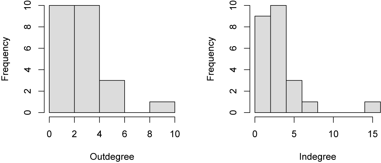
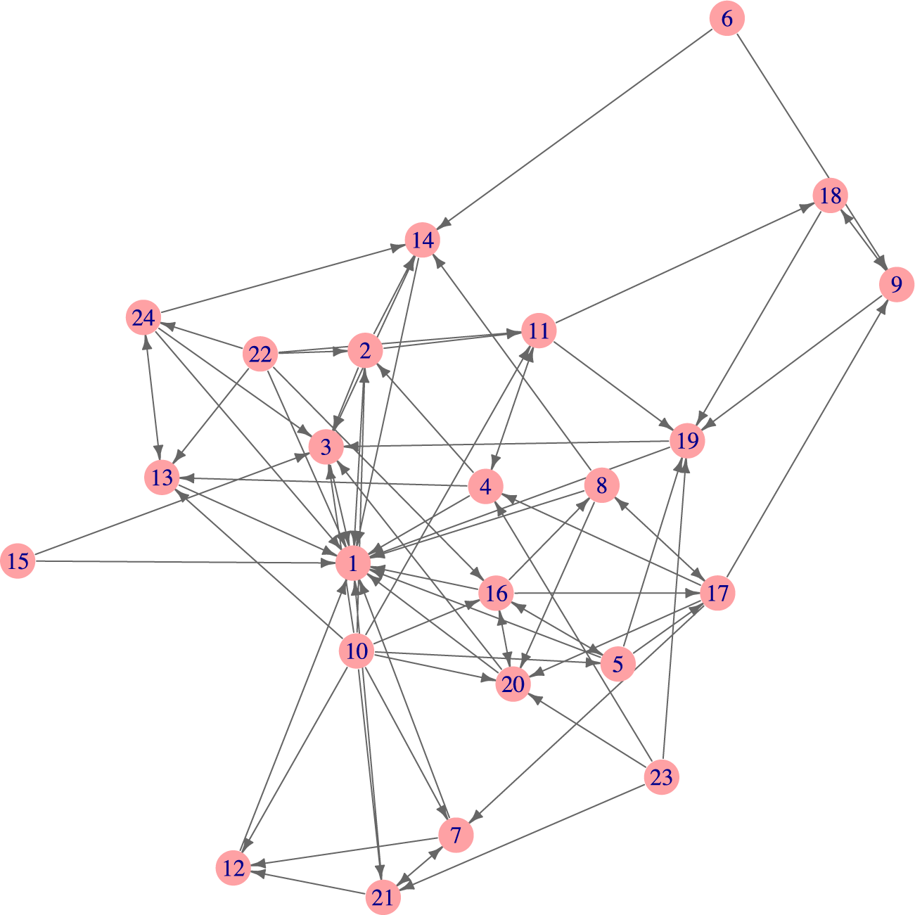
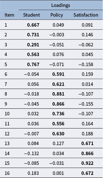
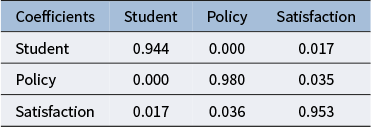
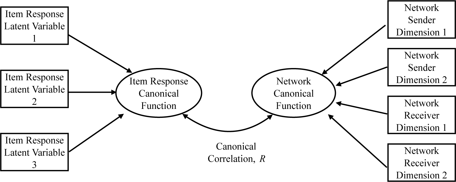
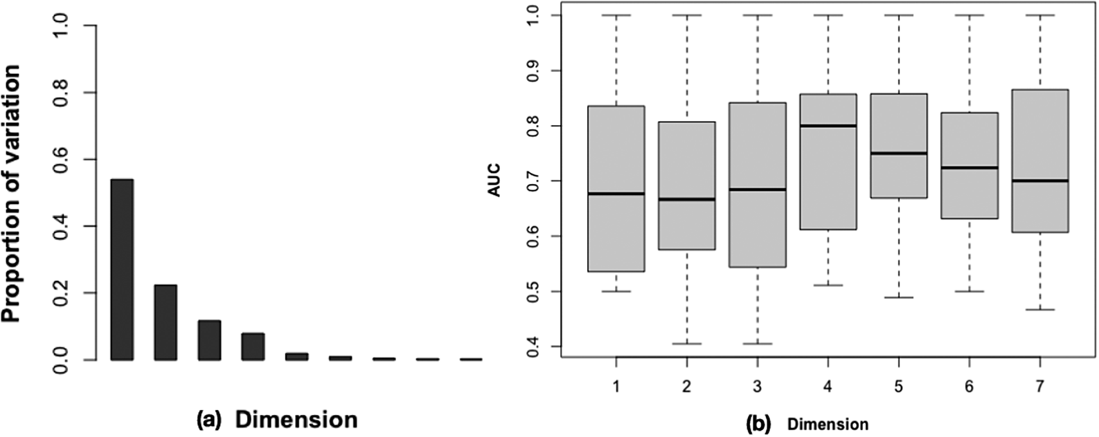
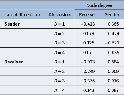

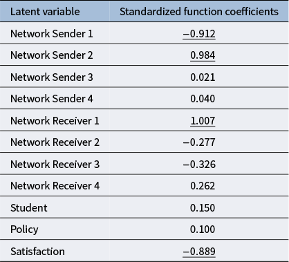
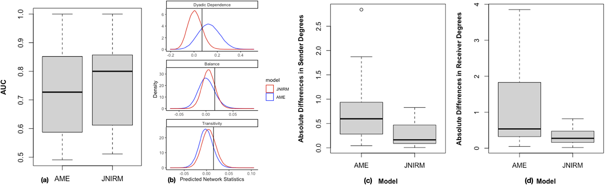
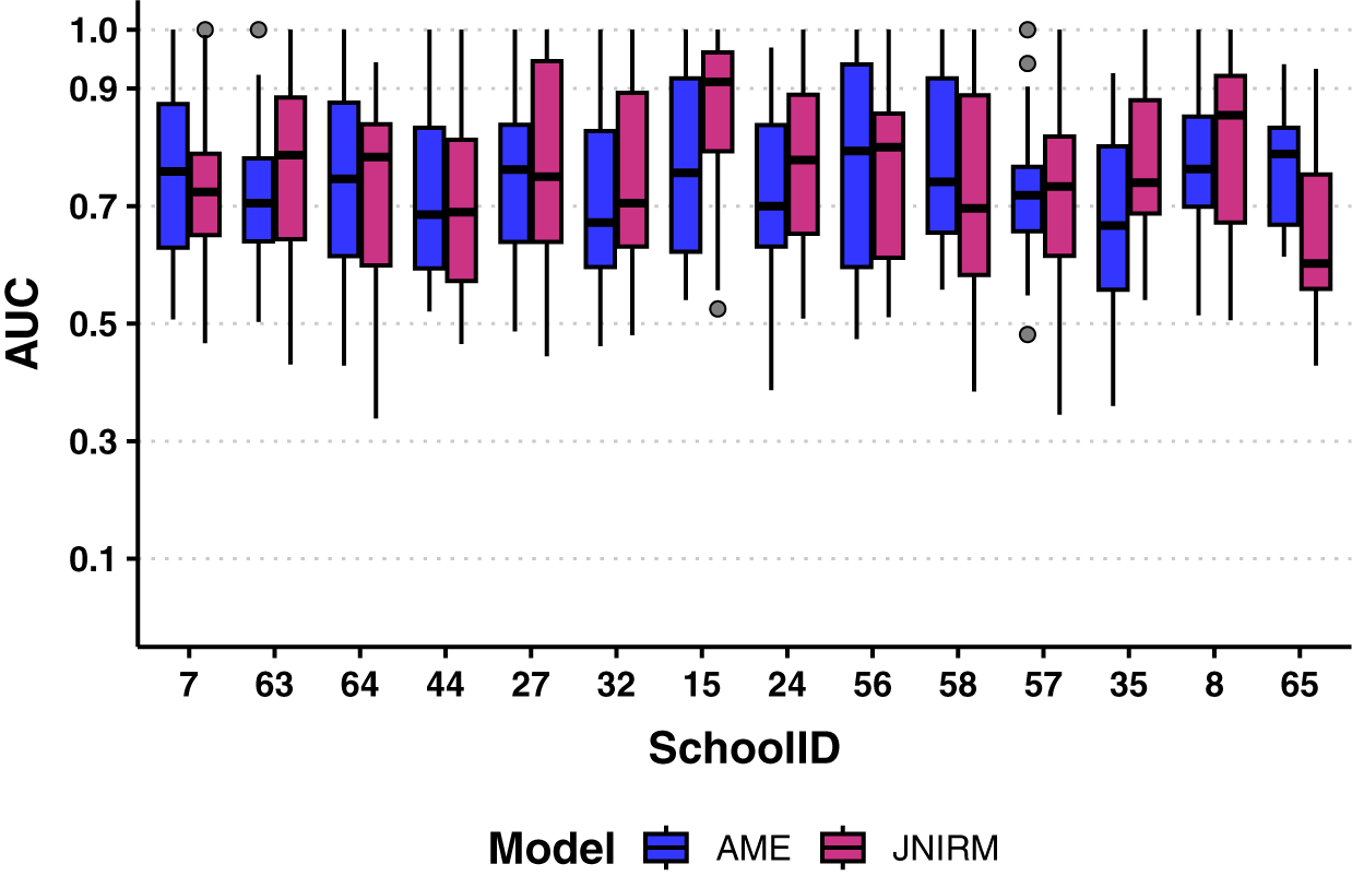
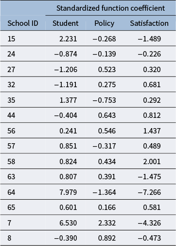
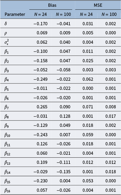
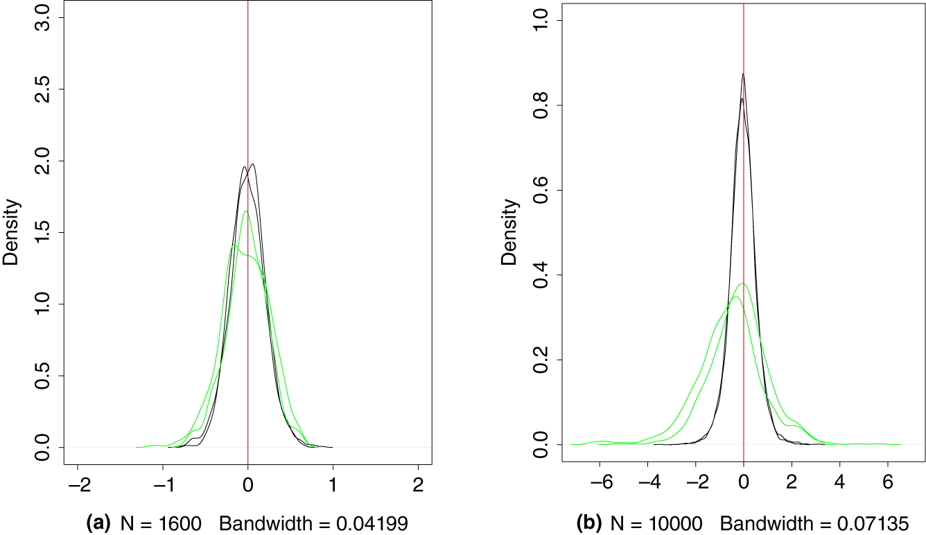


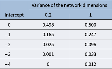
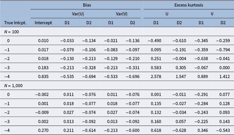


 Open access