


1. INTRODUCTION
Due to the changing climate and its implication on sea level, our ability to predict centennial-scale future ice-sheet behavior through modeling has received considerable attention (IPCC, 2013). These predictions are benefiting from an increasing amount of ground-based and remote-sensing observations and improving capabilities of ice-flow models. Advances in numerical methods and in computing power are starting to make full-order stress solutions of ice flow on ice-sheet scales possible (Larour and others, Reference Larour, Seroussi, Morlighem and Rignot2012; Khan and others, Reference Khan2015). Depending on the scientific questions, different data resolutions and model complexities are needed. For many questions, it is unclear whether additional data are needed or whether the model needs improvement. That is, to what extent would a finer grid of observations or a more complex model improve the ability to answer the question at hand.
Inverse methods are used to infer parameters from observations assuming a forward model that describes how the parameters are related to the observations. In our context, these are ill-posed problems, meaning that they do either not have a solution, have many (possibly infinitely many) solutions, or have unstable solutions. Instability is often the most critical factor and manifests itself in that a small change in observations can lead to a large change in the reconstructed parameters, which are often unphysical. It is therefore not desirable to find models that fit observations too accurately. In addition, errors in the forward model, that is the representation of the physical world with a set of partial differential equations, further complicate the problem, as these errors are often difficult to quantify. It is usually possible to stabilize the inversion by imposing additional constraints that bias the solution, a process that is generally referred to as regularization (e. g. Aster and others, Reference Aster, Borchers and Thurber2005). When the inversion is properly regularized, the field of data residuals, $ \Vert {d^{\rm {obs}} - d^{{\rm mod}}}\Vert $
, contains information about the error in the system. Residuals that are much larger than the expected errors in observations indicate problems in the ice-flow model assumptions, inputs, or geometry that are large enough to prevent a more accurate representation of observations when only one parameter can be adjusted.In this sense, residuals and residual patterns have the potential to identify sources of errors in a system, and to guide data collection and modeling strategies.
$ \Vert {d^{\rm {obs}} - d^{{\rm mod}}}\Vert $
, contains information about the error in the system. Residuals that are much larger than the expected errors in observations indicate problems in the ice-flow model assumptions, inputs, or geometry that are large enough to prevent a more accurate representation of observations when only one parameter can be adjusted.In this sense, residuals and residual patterns have the potential to identify sources of errors in a system, and to guide data collection and modeling strategies.
Jakobshavn Isbræ, one of the largest outlet glaciers on the west coast of Greenland has received a lot of attention due to its rapid changes in the beginning of this century (e.g. Thomas and others, Reference Thomas2003; Joughin and others, Reference Joughin, Abdalati and Fahnestock2004; Podlech and Weidick, Reference Podlech and Weidick2004). The importance of the dynamic behavior of outlet glaciers became clear and caused a surge of data campaigns and modeling efforts, especially for the Jakobshavn Isbræ drainage basin (e.g. Amundson and others, Reference Amundson2008; Holland and others, Reference Holland, Thomas, De Young, Ribergaard and Lyberth2008; Joughin and others, Reference Joughin2008; Motyka and others, Reference Motyka, Fahnestock and Truffer2010; Joughin and others, Reference Joughin2012). Nevertheless, Jakobshavn Isbræ remains a challenging glacier to study. The deep trough with its steep sides makes it difficult for radar surveys to receive clear bed returns (Bamber and others, Reference Bamber2013), and this ice geometry also makes it difficult to use simplified models that are based on shallowness. When inverting for basal conditions, the velocity residuals in the deep trough are larger than velocity observation errors (e.g. Gillet-Chaulet and others, Reference Gillet-Chaulet2012; Habermann and others, Reference Habermann, Truffer and Maxwell2013), and in this study we investigate if sources of error can be determined with the help of the residual pattern.
In Habermann and others (Reference Habermann, Truffer and Maxwell2013), basal yield stress inversions of Jakobshavn Isbræ for multiple years were performed and the changes in the first ~20 km from the terminus were examined. Here, we extend the area of interest but focus on the velocity residuals and residual patterns. In a series of synthetic experiments, the velocity residual pattern and magnitude for surface velocity, ice geometry, and modeling errors are examined. All these experiments concentrate on the terminus region (first ~100 km), where the residuals are high in real-data inversions.
Away from the terminus and the deep trough, residual values are small and the residual patterns suggest that the errors in velocity observations are the main cause for the mismatch. It is unclear, however, how far upstream basal yield stress can be resolved with present-day ice velocities. To address this question, we switch to drainage-basin-wide synthetic experiments to investigate the resolution strength with different checkerboard patterns of synthetic basal yield stress. Finally, real-data inversions are performed over the entire drainage basin, focusing on the sensitivity to different models and prior estimates. We discuss self-consistency of ice geometry and model, and how this affects inversion results.
2. METHODS
The quantitative model, also called ‘forward model’, describes how direct measurements, here surface velocities u, would be predicted from a set of physical parameters, here the basal yield stress τ c. The forward model thus contains a chosen simplification of ice flow, including some physical properties that are assumed to be known: ice softness A, Glen's flow law exponent n, density of ice ρ ice and gravitational acceleration g. Here, the geometry input fields are part of the forward model: ice thickness H and ice surface elevation z s are prescribed. Henceforth, we separate these effects and refer to the ice-flow simplification and the physical properties as the ‘model’ and we describe the ice-geometry input fields separately.
The Parallel Ice Sheet Model (PISM) is a three-dimensional (3-D) thermomechanically coupled ice-sheet model that solves a combination of the Shallow Ice and Shallow Shelf Approximations, here called the ‘hybrid model’ (Bueler and Brown, Reference Bueler and Brown2009). The Shallow Shelf Approximation (SSA) (Morland, Reference Morland, van der Veen and Oerlemans1987; MacAyeal, Reference MacAyeal1989) considers membrane (longitudinal and lateral) stresses and allows for sliding, while the Shallow Ice Approximation (SIA) considers a local stress-balance without sliding (Hutter, Reference Hutter1983). In PISM, the SSA and SIA are both calculated for each grid point and the modeled surface velocity is the sum of those two (Winkelmann and others, Reference Winkelmann2011). In this manner, the SSA is used as a ‘sliding law’ and the transition from mostly sliding to non-sliding occurs without inconsistencies or singularities.
The basal shear stress τ b is parametrized through a power law:
 $$\tau_{b} = \tau_{c} {\Vert {\bf u}\Vert^{{q-1}}\over u_{{\rm threshold}}^{q}} {\bf u}, $$
where u is the basal sliding velocity, and the threshold velocity u threshold is set to 100 m a−1. The purely plastic case is achieved by setting q = 0, whereas q = 1 leads to the common treatment of basal till as a linearly viscous material. Here, we solve for τ c, which has units of stress and is the basal yield stress if q = 0. In this study, we use q = 0.25, which has proven a good value for Greenland-wide calculations (Habermann and others, Reference Habermann, Truffer and Maxwell2013). While the chosen values for q and u threshold are somewhat arbitrary, we have checked a range of values and found the conclusions of this paper not to be very sensitive to the exact choice of q and u threshold.
We use the hybrid model in the inversion by first calculating SIA velocities u SIA from a given geometry and ice softness (the basal yield stress is not needed), and then subtracting u SIA from the observed surface velocities u obs. The inversion is then run with only the SSA forward model using a target velocity of
 $$ {\bf u}^{\rm target} = {\bf u}^{\rm obs} - {\bf u}^{\rm SIA}.$$
This approach is permissible and simple, because our hybrid model is a simple sum of the SIA and SSA velocities, which are treated as independent of each other (Winkelmann and others, Reference Winkelmann2011). Specifically, in our simplification the strain rates from one model do not affect the viscosity of the other. In synthetic SSA-only experiments, we generate u obs from an SSA forward model and set u target = u obs. The hybrid model is mainly applied in Section 3.4 where remote-sensing observations are used.
The inversion results in a modeled velocity u mod, which is the attempt to fit u target. The residual velocity is then defined as
 $$\Vert{ {\bf u}^{\rm target} - {\bf u}^{\rm mod}}\Vert.$$
This type of residual takes into account both the magnitude and the direction of the ice velocity. We also calculate a residual speed (difference in velocity magnitudes):
 $$\Vert{ {\bf u}^{\rm target}}\Vert - \Vert{ {\bf u}^{\rm mod}}\Vert.$$
In the ‘Results’ section, we will discuss both residuals.
We apply the widely used Tikhonov inversion, which defines a cost functional, I(τ c, α), with an added regularization term:
 $${\bf I}(\tau_{\rm c}, \alpha) = \alpha\, {\bf M}^2 + {\bf N}^2,$$
 $${\bf M}^2 = {1\over \Omega} \int_{\Omega} w\, \Vert {\bf u} (\tau_{\rm c}) - {\bf u}^{\rm target}\Vert^2 {\rm d}\Omega,$$
 $$ {\bf N}^2 = {1\over \Omega} \int_{\Omega} \Vert{\bf \nabla} (\tau_{\rm c} - \tau_{\rm c}^{{\rm prior}}) \Vert^2 {\rm d}\Omega,$$
where M is the data-model misfit, N is the model norm (regularization term), and α is the regularization parameter. The weight function w is introduced, so that the integrand is restricted to zero in areas of no observations. In the discrete form of the integral, it is zero at grid points that have no observed surface velocities, and one at all others. The area Ω is defined by grounded ice (determined by hydrostatic equilibrium). Additionally a 10 km (~10 H) border around the model domain boundary is not contained in the misfit area. The velocities in this border domain are strongly influenced by stresses outside the domain, so fitting velocities there might produce unphysical results. The model norm in Eqn (7) is a Sobolev H 1 norm, which biases the solution toward smooth differences to the prior estimate. That is, the regularization tends to preserve the roughness of the prior estimate. Different model norms or combinations of model norms are possible as outlined in Habermann and others (Reference Habermann, Truffer and Maxwell2013). The L-curve method is applied to find the appropriate value for α: the data-model misfit is plotted against the model norm, this curve typically has an L-shape and the regularization parameter value corresponding to the ‘corner’ of the curve is chosen (Aster and others, Reference Aster, Borchers and Thurber2005, p. 91). The rationale behind this choice of regularization parameter is that past this corner even a small improvement in the data-model misfit can only be achieved through a large increase in the model norm (e.g. the roughness of the solution).
In the first part of this study, synthetic experiments are performed where a given basal yield stress, $ \tau _{\rm c}^{\rm {synth}} $
, is used in a forward model to produce a surface velocity field, u
synth. Different versions of the forward model are used here, with different model simplifications, physical properties or geometry input fields. The synthetic surface velocity is then applied as u
target in an inversion, either as is, or with added noise.
$ \tau _{\rm c}^{\rm {synth}} $
, is used in a forward model to produce a surface velocity field, u
synth. Different versions of the forward model are used here, with different model simplifications, physical properties or geometry input fields. The synthetic surface velocity is then applied as u
target in an inversion, either as is, or with added noise.
All synthetic experiments are then inverted for τ
c, which can then be compared with $ \tau _{\rm c}^{\rm synth} $
. We define the ice geometry with the bed topography from Gogineni (Reference Gogineni2012) and a 2006 surface DEM. This 2006 DEM is produced with a 2007 DEM (Motyka and others, Reference Motyka, Fahnestock and Truffer2010) and annual elevation-difference maps from Joughin and others (Reference Joughin2012) for ~100 km around the terminus. In the remainder of the drainage basin, we used the Bamber and others (Reference Bamber, Layberry and Gogineni2001) DEM (for details see Habermann and others (Reference Habermann, Truffer and Maxwell2013)). The prior estimate for the basal yield stress is set to
$ \tau _{\rm c}^{\rm synth} $
. We define the ice geometry with the bed topography from Gogineni (Reference Gogineni2012) and a 2006 surface DEM. This 2006 DEM is produced with a 2007 DEM (Motyka and others, Reference Motyka, Fahnestock and Truffer2010) and annual elevation-difference maps from Joughin and others (Reference Joughin2012) for ~100 km around the terminus. In the remainder of the drainage basin, we used the Bamber and others (Reference Bamber, Layberry and Gogineni2001) DEM (for details see Habermann and others (Reference Habermann, Truffer and Maxwell2013)). The prior estimate for the basal yield stress is set to $ \tau _{\rm c}^{\rm {prior}} = 1 . 4 \times 10^{5} $
Pa, the H
1 norm is used as the model norm N, the Glen's flow law parameter is set to n = 3, and the ice softness is set to A = 2.5 × 10⁻²⁴ Pa−3 s−1. This corresponds to an ice hardness of B = A
−1/3 = 0.7 × 10⁸ Pas1/3. According to the values recommended by Cuffey and Paterson (Reference Cuffey and Paterson2010), the rate factor corresponds to a relatively high temperature of 270 K. A justification for these choices is provided in Habermann and others (Reference Habermann, Truffer and Maxwell2013). We use the SSA as a forward model and call this setup the ‘reference’ inversion, with reference ice-geometry and physical properties.
$ \tau _{\rm c}^{\rm {prior}} = 1 . 4 \times 10^{5} $
Pa, the H
1 norm is used as the model norm N, the Glen's flow law parameter is set to n = 3, and the ice softness is set to A = 2.5 × 10⁻²⁴ Pa−3 s−1. This corresponds to an ice hardness of B = A
−1/3 = 0.7 × 10⁸ Pas1/3. According to the values recommended by Cuffey and Paterson (Reference Cuffey and Paterson2010), the rate factor corresponds to a relatively high temperature of 270 K. A justification for these choices is provided in Habermann and others (Reference Habermann, Truffer and Maxwell2013). We use the SSA as a forward model and call this setup the ‘reference’ inversion, with reference ice-geometry and physical properties.
2.1. Data
For the inversions in Sections 3.1 and 3.2, where our analysis is limited to the terminus area, we use NASA's Making Earth System Data Records for Use in Research Environments (MEaSUREs) velocity map for the winter 2006/07 (Joughin and others, Reference Joughin, Smith, Howat, Scambos and Moon2010a, Reference Joughin, Smith, Howat and Scambosb). In later inversions of the entire drainage basin, we prefer a more complete data set of surface velocities, and therefore, we use an average of winter velocities for 2000, 2006–2009 (Joughin and others, Reference Joughin, Smith, Howat, Scambos and Moon2010b). The reference inversion is performed with the bed topography given by an earlier version of Jakobshavn Isbræ's bed (Gogineni, Reference Gogineni2012). In Section 3.1, we use a newer bed topography data set (Gogineni, Reference Gogineni2014) to simulate the effects of possible errors in bed topography.
3. EXPERIMENTS
In Section 3.1, velocity residuals are investigated and we use a model domain limited to the terminus area of Jakobshavn Isbræ. Experiments on this limited model domain are performed on a uniform 500 m × 500 m grid. In later sections, the entire drainage basin is used, as determined from the surface topography and an assumption of downhill ice flow. We expand the drainage basin to make it a rectangular domain that contains it entirely, and solutions are found on this simpler domain. Inversions on this larger rectangular domain are performed on a uniform 1 km × 1 km grid. For the limited model domain, we assume a constant ice softness; for the entire domain we tested constant ice softness as well as ice softness fields derived from spin-ups. Numerical experiments on the limited domain are listed in Tables 1, and Table 2 lists the parameters of the full domain experiments.
Summary of synthetic residual pattern experiments performed on the limited domain. ‘Ref.’ refers to the reference inversion: geometry given by bed topography from Gogineni (Reference Gogineni2012) and the 2006 surface DEM described in Habermann and others (Reference Habermann, Truffer and Maxwell2013). The Glen's flow law exponent is set to n = 3, the ice softness is set to A = 2.5 × 10⁻²⁴ Pa−3 s−1 and the SSA as a forward model
Summary of real-data, drainage-basin-wide τ c inversions shown in Figure 12. For all inversions the averaged velocity described in Section 2.1, the H 1 model norm, and a regularization parameter found with the L-curve method is used. ‘Ref.’ refers to the reference inversion described in Section 2
3.1. Velocity residual pattern
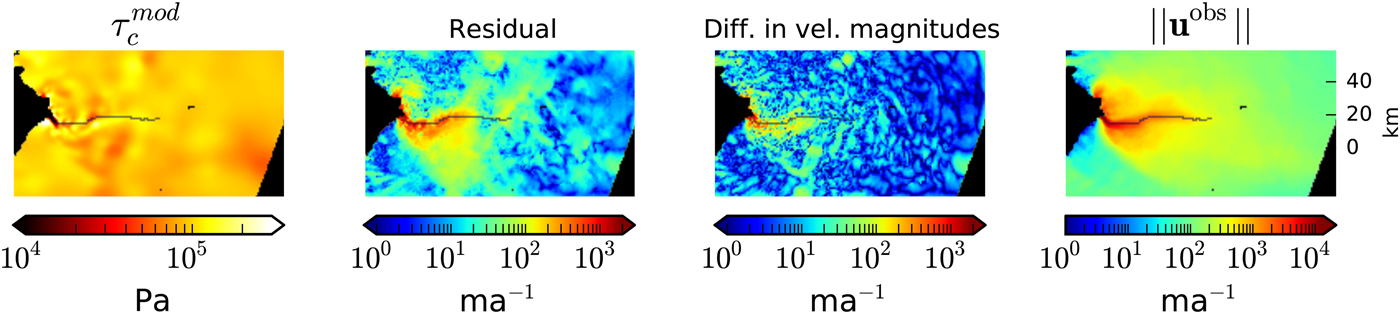
In Habermann and others (Reference Habermann, Truffer and Maxwell2013), we show that even though the residuals in the trough close to the terminus are high, the relative residuals in the area of interest when studying the rapid changes close to the terminus are small. When we restrict ourselves to the 2006 inversion, but extend our field of view and plot the residuals on a log scale, distinct patterns in residual become apparent (Fig. 1). With the following set of experiments, we investigate which of the possible sources of error is most likely causing these residual patterns.
Real-data inversion and residual pattern for the 2006 surface velocities. The columns show modeled basal yield stress, residual ( $ \Vert {\bf u}^{\rm obs} - {\bf u}^{\rm mod}\Vert $
), difference in velocity magnitudes (
$ \Vert {\bf u}^{\rm obs} - {\bf u}^{\rm mod}\Vert $
), difference in velocity magnitudes ( $\vert \Vert {\bf u}^{\rm obs}\Vert - \Vert {\bf u}^{\rm mod}\Vert$
) and observed velocities. The black line delineates the glacier's centerline and black dots show data gaps.
$\vert \Vert {\bf u}^{\rm obs}\Vert - \Vert {\bf u}^{\rm mod}\Vert$
) and observed velocities. The black line delineates the glacier's centerline and black dots show data gaps.
We run forward models to produce a series of target velocity fields u
target with different input parameters, geometries, or forward models. We also investigate the effect of adding noise to these model outputs. The specifics of the ten experiments are given in Table 1. For all experiments in this section, $ {\tau}_{\rm c}^{\rm synth}$
is set to the
$ {\tau}_{\rm c}^{\rm synth}$
is set to the ${\tau}_{\rm c}^{\rm mod} $
in Figure 1. The different u
target are then used in a reference inversion and the resulting
${\tau}_{\rm c}^{\rm mod} $
in Figure 1. The different u
target are then used in a reference inversion and the resulting ${\tau}_{\rm c}^{\rm mod}$
and velocity residuals are investigated.
${\tau}_{\rm c}^{\rm mod}$
and velocity residuals are investigated.
3.1.1. Surface velocity errors
First, the influence of noise in the surface velocity observations is examined. For all four experiments in this category the reference ice geometry and model are used to produce u synth, and then different types of noise are added (Table 1). Experiment 1 is performed without added noise for comparison. In experiment 2, we add a Gaussian distribution for random uncorrelated surface velocity errors with standard deviation (std dev.) of 5 m a−1. Experiment 3 uses a Gaussian distribution of surface velocity errors that is scaled with 1% of the magnitude of the surface velocities (u synth). In experiment 4, we use the actual reported errors, smoothed with a 1 km Gaussian kernel.
Figure 2 shows results for all four experiments. Experiments 2 and 3 reproduce ${\tau}_{\rm c}^{\rm synth} $
very well, with larger discrepancies in the trough close to the terminus for experiment 3 and in the slow flow areas for experiment 2. When mimicking the velocity errors given in the observations (exp. 4) the relative difference between
${\tau}_{\rm c}^{\rm synth} $
very well, with larger discrepancies in the trough close to the terminus for experiment 3 and in the slow flow areas for experiment 2. When mimicking the velocity errors given in the observations (exp. 4) the relative difference between ${\tau}_{\rm c}^{\rm mod}$
and
${\tau}_{\rm c}^{\rm mod}$
and ${\tau}_{\rm c}^{\rm synth}$
increases even though the residual pattern suggests a better fit than in experiment 2. The residual pattern mirrors the pattern of added velocity error in all three experiments. The area of high relative residual (white area) on rock-terminating ice on either side of the Jakobshavn Isbræ terminus for experiments 2 and 4 suggests that high relative velocity errors in these slow-flowing areas largely affect the ability to match the target velocities.
${\tau}_{\rm c}^{\rm synth}$
increases even though the residual pattern suggests a better fit than in experiment 2. The residual pattern mirrors the pattern of added velocity error in all three experiments. The area of high relative residual (white area) on rock-terminating ice on either side of the Jakobshavn Isbræ terminus for experiments 2 and 4 suggests that high relative velocity errors in these slow-flowing areas largely affect the ability to match the target velocities.
Synthetic inversions with errors in observations. The columns show the relative τ
c difference ( $(\Vert{\tau}_{\rm c}^{\rm synth} - {\tau}_{\rm c}^{\rm mod}\Vert)/{\tau}_{\rm c}^{\rm synth} $
), the residual (
$(\Vert{\tau}_{\rm c}^{\rm synth} - {\tau}_{\rm c}^{\rm mod}\Vert)/{\tau}_{\rm c}^{\rm synth} $
), the residual ( $ \Vert {\bf u}^{\rm target} - {\bf u}^{\rm mod}\Vert $
), the difference in velocity magnitudes (
$ \Vert {\bf u}^{\rm target} - {\bf u}^{\rm mod}\Vert $
), the difference in velocity magnitudes ( $ \vert \Vert { {\bf u}^{\rm target}}\Vert - \Vert { {\bf u}^{\rm mod}}\Vert $
), and the added velocity error (
$ \vert \Vert { {\bf u}^{\rm target}}\Vert - \Vert { {\bf u}^{\rm mod}}\Vert $
), and the added velocity error ( $ \Vert {\bf u}^{\rm target}\Vert - \Vert {\bf u}^{\rm synth}\Vert $
). The rows show the different experiments: (1) inversion without added error (for comparison), (2) Gaussian noise of rms 5 m a−1 added, (3) Gaussian noise scaled to velocity, and (4) noise according to the error values given in the observation file.
$ \Vert {\bf u}^{\rm target}\Vert - \Vert {\bf u}^{\rm synth}\Vert $
). The rows show the different experiments: (1) inversion without added error (for comparison), (2) Gaussian noise of rms 5 m a−1 added, (3) Gaussian noise scaled to velocity, and (4) noise according to the error values given in the observation file.

The four experiments discussed here reach very low data-model misfit values. This can be seen in the L-curves (Fig. 6), which show the misfit as a function of the regularizing model norm. The asymptotic value of the L-curve indicates how well observations can be fit. We conclude that realistic amounts of surface velocity errors can only account for a small amount of the data-model misfit that is observed in real-data inversions. Because the u synth is known in these synthetic experiments, the data-model misfit can be calculated directly; for experiment 2, this value is shown in the inset of Figure 6.
3.1.2. Ice-geometry errors
In a second set of experiments, we investigate the influence of errors in the surface elevation and the bed topography. In experiment 5, we add a Gaussian distribution of uncorrelated random noise with std dev. of 5 m to the surface elevation before calculating the synthetic surface velocities. In experiment 6, the CReSIS bed elevation is used. The differences between the reference fields (surface elevation and bed topography) and the synthetic fields are shown in the far-right column of Figure 3. As for all other synthetic experiments, the reference inversion (model and input fields) is then used to find $ \tau_{\rm c}^{\rm mod}$
.
$ \tau_{\rm c}^{\rm mod}$
.
Synthetic inversions with errors in ice geometry. The columns show the relative τ
c difference ( $ \Vert \tau _{\rm c}^{\rm synth} - \tau _{\rm c}^{\rm mod}\Vert / \tau _{\rm c}^{\rm synth} $
), the residual (
$ \Vert \tau _{\rm c}^{\rm synth} - \tau _{\rm c}^{\rm mod}\Vert / \tau _{\rm c}^{\rm synth} $
), the residual ( $ \Vert {\bf u}^{\rm target} - {\bf u}^{\rm mod}\Vert $
), the difference in velocity magnitudes (
$ \Vert {\bf u}^{\rm target} - {\bf u}^{\rm mod}\Vert $
), the difference in velocity magnitudes ( $ \vert \Vert { {\bf u}^{\rm target}}\Vert - \Vert { {\bf u}^{\rm mod}}\Vert $
), and the added geometry error in ice surface elevation/bed topography for experiments 5/6. The rows show results for experiments (5) added error in ice surface elevation (Gaussian distribution of uncorrelated random noise withstd dev. of 5 m), (6) added error in bed topography by using a newer bed topography for the forward model and an older bed topography for the inversion.
$ \vert \Vert { {\bf u}^{\rm target}}\Vert - \Vert { {\bf u}^{\rm mod}}\Vert $
), and the added geometry error in ice surface elevation/bed topography for experiments 5/6. The rows show results for experiments (5) added error in ice surface elevation (Gaussian distribution of uncorrelated random noise withstd dev. of 5 m), (6) added error in bed topography by using a newer bed topography for the forward model and an older bed topography for the inversion.

Figure 3 shows the results for these two experiments. The residual fields show higher residuals in the areas close to the terminus, suggesting that ice-geometry errors lead to larger residuals in the fast-flow areas compared with slow flow areas. The large topography errors in the upstream area (bottom right corner of the residual plot in Fig. 3) are also reflected in the residual field. The modeled basal yield stress fields for both experiments show large deviations from the synthetic value because they compensate for the errors in geometries. It is surprising how similar the deviations from $ \tau _{\rm c}^{\rm synth} $
are for experiments 5 and 6 despite the vastly different errors that are introduced in the geometries. A common pattern is that
$ \tau _{\rm c}^{\rm synth} $
are for experiments 5 and 6 despite the vastly different errors that are introduced in the geometries. A common pattern is that $ \tau _{\rm c}^{\rm mod} $
is lowered in the deep trough. In the area close to the terminus, where the glacier has a bend, the modeled basal yield stress switches from being higher than
$ \tau _{\rm c}^{\rm mod} $
is lowered in the deep trough. In the area close to the terminus, where the glacier has a bend, the modeled basal yield stress switches from being higher than $ \tau _{\rm c}^{\rm synth} $
to lower than
$ \tau _{\rm c}^{\rm synth} $
to lower than $ \tau _{\rm c}^{\rm synth} $
in an attempt to match the observed velocities despite the wrong ice geometry.
$ \tau _{\rm c}^{\rm synth} $
in an attempt to match the observed velocities despite the wrong ice geometry.
Figure 6 shows L-curves for experiments 5 and 6 with sharp corners. This shape is in contrast to the shape of the L-curve for the real-data inversion, and suggests that errors in ice geometry alone cannot recreate the shape of the real-data L-curve. The surface elevation errors lead to similarly low data-model misfit values (~6 m a−1) as experiments 2–4, whereas the experiment with topography errors leads to data-model misfit values of about 30 m a−1. For both ice-geometry error experiments the L-curves begin at high data-model misfits and descend rapidly, creating sharp corners that make it easy to choose the regularization parameter, nonetheless even with the large errors in topography the data-model misfit is still lower than in the real-data inversion.
3.1.3. Ice-temperature errors
Next, we investigate the influence of ice-temperature errors on the inversion results. The temperature affects the hardness of the ice through the flow law. In this experiment, we run a forward model with a spatially-varying ice temperature field from a constant-climate spin-up performed with PISM as outlined in Aschwanden and others (Reference Aschwanden, Adalgeirsdóttir and Khroulev2013). The resulting depth-averaged PISM ice hardness field is shown in the far-right column of Figure 4. These values are almost an order of magnitude higher than the reference run, corresponding to temperatures about 10 K lower. While this is quite a large difference, the forward model values are not unrealistic, given measurements further upstream (Funk and others, Reference Funk, Echelmeyer and Iken1994; Lüthi and others, Reference Lüthi, Funk, Iken, Truffer and Gogineni2002). As for all other synthetic experiments, the reference inversion (model and input fields) with a constant ice temperature is used in the inversion to find $ \tau_{\rm c}^{\rm mod}$
.
$ \tau_{\rm c}^{\rm mod}$
.
Synthetic inversions simulating errors in ice temperature. The columns show the relative τ
c difference ( $ \Vert \tau _{\rm c}^{\rm synth} - \tau _{\rm c}^{\rm mod}\Vert / \tau _{\rm c}^{\rm synth} $
), the residual (
$ \Vert \tau _{\rm c}^{\rm synth} - \tau _{\rm c}^{\rm mod}\Vert / \tau _{\rm c}^{\rm synth} $
), the residual ( $ \Vert {\bf u}^{\rm target} - {\bf u}^{\rm mod}\Vert $
), the difference in velocity magnitudes (
$ \Vert {\bf u}^{\rm target} - {\bf u}^{\rm mod}\Vert $
), the difference in velocity magnitudes ( $ \vert \Vert { {\bf u}^{\rm target}}\Vert - \Vert { {\bf u}^{\rm mod}}\Vert $
), and the ice hardness field used in the forward model. The inversion was performed with a spatially uniform hardness.
$ \vert \Vert { {\bf u}^{\rm target}}\Vert - \Vert { {\bf u}^{\rm mod}}\Vert $
), and the ice hardness field used in the forward model. The inversion was performed with a spatially uniform hardness.
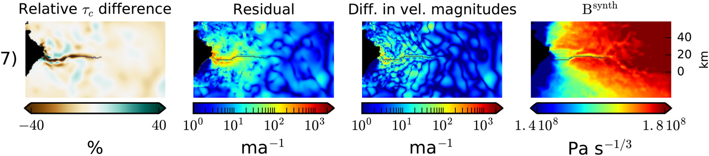
Figure 4 shows the result of the experiment with ice-temperature errors. The ice hardness used in the forward run was generally higher than in our reference model and the inverted $ \tau _{\rm c}^{\rm mod} $
is compensating with lower values compared with
$ \tau _{\rm c}^{\rm mod} $
is compensating with lower values compared with $ \tau _{\rm c}^{\rm synth} $
. Looking at the residual patterns, we see the highest widespread residual of all the synthetic experiments, so far. But the residual values in the deep trough are still not as high as in the real-data inversion. It is also noticeable that the difference in velocity magnitudes shows a clear improvement over the residuals, indicating that the inversion struggles to match the velocity directions.
$ \tau _{\rm c}^{\rm synth} $
. Looking at the residual patterns, we see the highest widespread residual of all the synthetic experiments, so far. But the residual values in the deep trough are still not as high as in the real-data inversion. It is also noticeable that the difference in velocity magnitudes shows a clear improvement over the residuals, indicating that the inversion struggles to match the velocity directions.
3.1.4. Model errors
Lastly, errors in the ice-flow model are investigated. In experiment 8, the exponent in Glen's flow law is set to n = 2.5 and the constant ice softness is adjusted to A = 1.7 × 10⁻²¹ Pa−3 s−1 according to Funk and others (Reference Funk, Echelmeyer and Iken1994). For experiment 9 the synthetic surface velocities are produced with the reference ice geometry and model, but u SIA is added before the inversion. Again, the inversion itself is then performed with the reference values (SSA-only, n = 3 and A = 2.5 × 10⁻²⁴ Pa−3 s−1).
In the last experiment, we used a forward run with the Full-Stokes Elmer/Ice model (Gagliardini and others, Reference Gagliardini2013) and performed the inversion with our SSA-only ice-flow model. Here the 1 km SEARISE topography and ice thickness were used, while the enthalpy field used in the forward and the inverse run are from a SICOPOLIS spin-up (Bindschadler and others, Reference Bindschadler2013). The inversion deviates from the reference inversion used in the other experiments in an attempt to keep as many variables as possible constant between the forward and inverse run with the goal of highlighting the potential mismatch solely due to a simplified model in the inversion.
Figure 5 shows that errors in the model can strongly affect the ability to match the target velocities. The residuals are high and widespread and the patterns in experiment 8 resemble the residuals in real-data inversions. Despite the large deviations of basal yield stress from the target values, the target velocities cannot be matched well. Experiment 9 displays the typical wave-like patterns that arise from the u SIA calculation. This pattern is visible in the residual as well as in the difference u ref − u target and will be discussed in the next section. Note that the wave-like pattern in residual in experiment 9 is not visible in the real-data inversion. Experiment 10 results in high residuals in the fast-flow area, that are comparable with the real-data residuals. The pattern of residuals in the slow-flow areas, however, does not resemble the real-data residuals.
Synthetic inversions with errors in ice-flow model. The columns show the relative τ
c difference ( $ \Vert \tau _{\rm c}^{\rm synth} - \tau _{\rm c}^{\rm mod}\Vert /\Vert \tau _{\rm c}^{\rm synth}\Vert $
), the residual (
$ \Vert \tau _{\rm c}^{\rm synth} - \tau _{\rm c}^{\rm mod}\Vert /\Vert \tau _{\rm c}^{\rm synth}\Vert $
), the residual ( $ \Vert {\bf u}^{\rm target} - {\bf u}^{\rm mod}\Vert $
), the difference in velocity magnitudes (
$ \Vert {\bf u}^{\rm target} - {\bf u}^{\rm mod}\Vert $
), the difference in velocity magnitudes ( $ \vert \Vert { {\bf u}^{\rm target}}\Vert - \Vert { {\bf u}^{\rm mod}}\Vert $
), and the difference between
$ \vert \Vert { {\bf u}^{\rm target}}\Vert - \Vert { {\bf u}^{\rm mod}}\Vert $
), and the difference between $ \Vert {\bf u}^{\rm target}\Vert $
used in the inversion and
$ \Vert {\bf u}^{\rm target}\Vert $
used in the inversion and $ \Vert {\bf u}^{\rm ref}\Vert $
which is the velocity resulting from the reference forward model. The rows show results for experiments (8): u
target produced with a Glen's flow law constant set to n = 2.5 and the ice softness set accordingly to A = 1 × 10⁻²¹ Pa−3 s
−1, (9): u
target produced by adding SIA velocities to u
synth, (10): u
target produced in a forward run with the Elmer/Ice model.
$ \Vert {\bf u}^{\rm ref}\Vert $
which is the velocity resulting from the reference forward model. The rows show results for experiments (8): u
target produced with a Glen's flow law constant set to n = 2.5 and the ice softness set accordingly to A = 1 × 10⁻²¹ Pa−3 s
−1, (9): u
target produced by adding SIA velocities to u
synth, (10): u
target produced in a forward run with the Elmer/Ice model.

3.1.5. Discussion of residual pattern experiments
An investigation of the residual patterns shows that the bed topography experiment (Exp. 6) has high residual values in the fast-flowing terminus region, although they do not reach the widespread values of 50–100 m a−1 seen in the real-data inversion. The difference between the two bed topography fields is largest in the deep trough, which is the area where actual uncertainties in bed topography are expected to be large because of the difficult recovery of bed radar returns. In this sense, our experiment represents a realistic assumption about bed topography uncertainties and we expect similar residual patterns for actual uncertainties in bed topography. The model error experiment (Exp. 8) is the only one with the characteristic widespread pattern of 50–100 m a−1 residuals, but the residuals in the deep trough are still not as high as in the real-data inversion.
Figure 6 shows that only experiments 9 and 10 reach the high data-model misfit values, which we see in the real-data inversions. The residual patterns on the other hand, show that the high residuals in the hybrid model experiment are due to the addition of unrealistic SIA velocities. The widespread high residual pattern of experiment 8 is very similar to the real-data inversion, but the L-curve shows that the data-model misfit over the entire misfit area is still too low. Adding the residuals from the bed topography experiment (Exp. 6) would lead to a data-model misfit value that is closer to the real-data inversion. The flat shape of the L-curve occurs for both model error and the ice-temperature experiments. This makes it difficult to find a clear corner, which introduces additional uncertainties into the inversion results. But this is also the case for real-data inversions, so we are able to reproduce the residual patterns and the shape of the L-curve of the real-data inversion.
L-curves for all velocity residual pattern experiments. The bold dots mark the inversions that are shown in the map-view figures above for each experiment. The blue line in the inset shows the calculated data-model misfit for experiment 2.
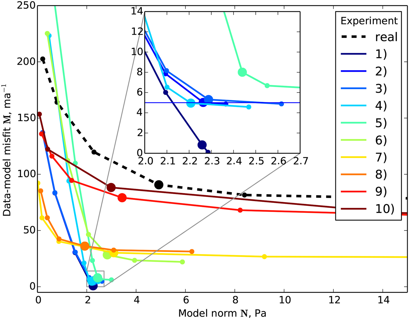
Experiment 9 displays a distinct wave-like pattern in residuals. This wave-like pattern is a result of wave-like SIA velocity fields that cannot be achieved with the SSA-only inversion. The wave-like features most likely represent the mismatch between bed topography and surface elevations. If both of these fields would be perfect, the SIA would produce a wrong surface velocity field (because the SIA is not necessarily a good model simplification), but this velocity field would not display such a distinct wave-like pattern. When running the hybrid model forward in time and allowing the surface to evolve, these wave-like patterns in SIA velocities smooth out. This in turn, reduces the wave-like patterns in the residual fields when using the evolved surface instead of the measured surface elevations in the inversion (see Section 3.4).
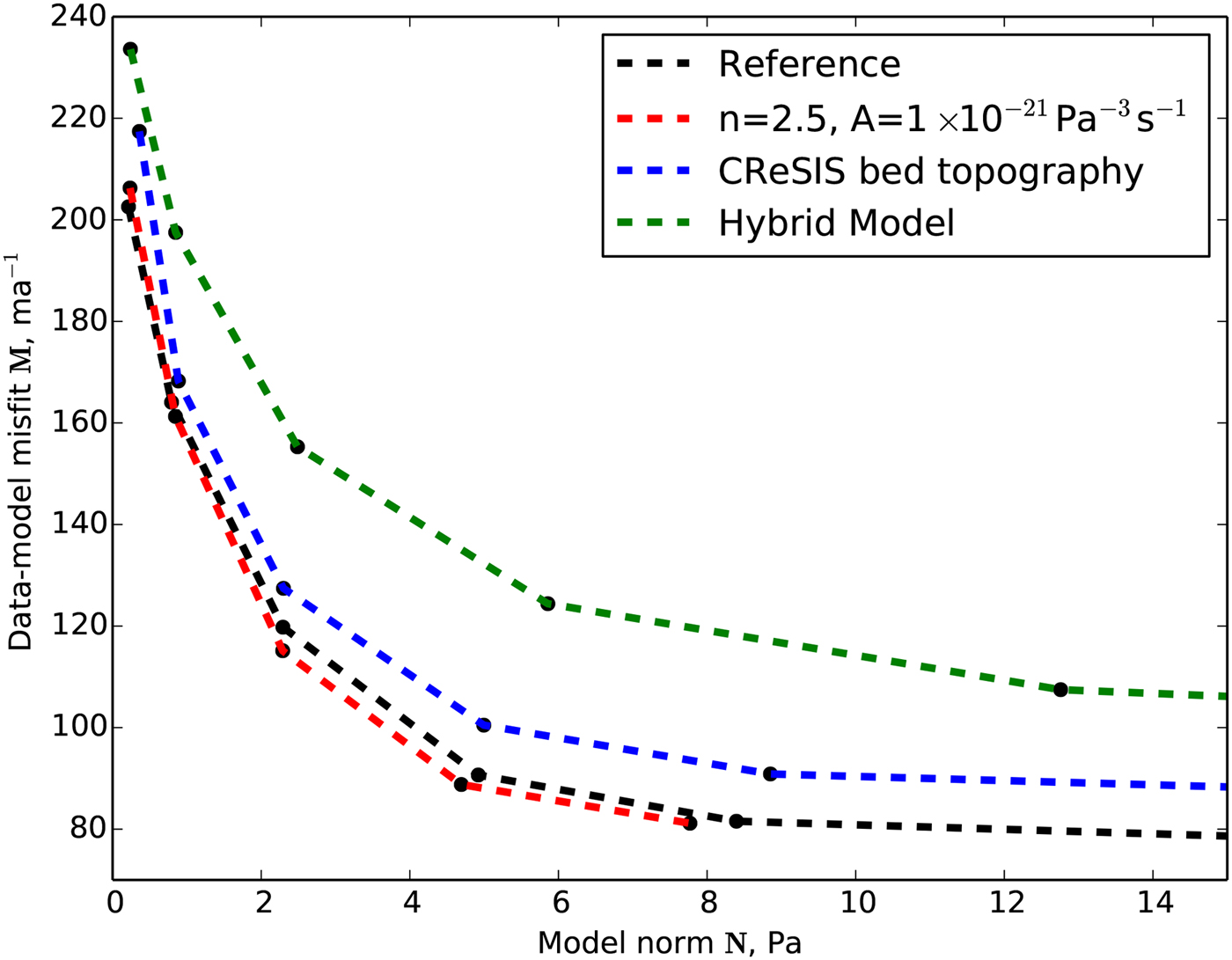
The synthetic experiments might suggest that the real-data inversions could be improved by using the newer CReSIS bed topography, or a model that uses a Glen's flow law parameter of n = 2.5 with an adjusted ice softness, which has been suggested to be a better choice for the Jakobshavn Isbræ (Funk and others, Reference Funk, Echelmeyer and Iken1994). Inspection of the L-curves for these inversions shows, however, that the CReSIS topography actually increases the data-model misfit and that the improvement when using n = 2.5 is negligible (Fig. 7). The residual patterns for these real-data inversions (not shown) are almost indistinguishable from the pattern in Figure 1. The hybrid model applied to the real-data inversion leads to higher data-model misfit values than the reference inversion. We conclude that even with the newest bed topography and an adjusted Glen's flow law parameter, the residual patterns are not significantly improved. Therefore, we conclude that even further improvements in bed topography data and/or more complex models are necessary for an improved data-model misfit in the terminus region.
L-curves for real-data inversions with different model and ice geometry.
3.2. Weighted misfit function
In the experiments discussed above, all points within the misfit area have been equally weighted, regardless of the magnitude of velocity or the expected error at that point. Morlighem and others (Reference Morlighem2010) suggested that such unweighted cost functionals work better in fast-flow areas because the gradients of the misfit functional are larger where $ \Vert {\bf u}^{\rm target} - {\bf u}^{\rm mod}\Vert $
is high, which occurs in regions of fast flow. According to this, a misfit functional that weights the slow flow areas stronger would lead to improved resolution of basal yield stress there. Here, we test the resolution strength of weighted and unweighted misfit functionals.
$ \Vert {\bf u}^{\rm target} - {\bf u}^{\rm mod}\Vert $
is high, which occurs in regions of fast flow. According to this, a misfit functional that weights the slow flow areas stronger would lead to improved resolution of basal yield stress there. Here, we test the resolution strength of weighted and unweighted misfit functionals.
We perform so-called checkerboard tests, a common technique in geophysical research (e.g. Thorsteinsson and others, Reference Thorsteinsson2003; Koulakov and others, Reference Koulakov2012). The checkerboard pattern of basal yield stress is produced by taking $ \tau _{\rm c}^{\rm mod} $
from Figure 1 and overlaying it with lateral and longitudinal variations of basal yield stress with a certain amplitude and wavelength. In cases where the amplitude of the checkerboard pattern would cause negative values of basal yield stress, τ
c is set to zero. This checkerboard pattern is used in a SSA forward model to get u
synth, Gaussian noise is added and the resulting u
target is used in the inversion.
$ \tau _{\rm c}^{\rm mod} $
from Figure 1 and overlaying it with lateral and longitudinal variations of basal yield stress with a certain amplitude and wavelength. In cases where the amplitude of the checkerboard pattern would cause negative values of basal yield stress, τ
c is set to zero. This checkerboard pattern is used in a SSA forward model to get u
synth, Gaussian noise is added and the resulting u
target is used in the inversion.
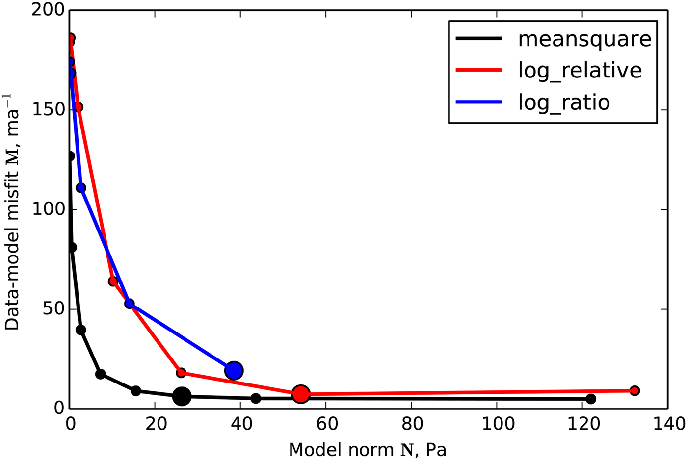
Checkerboard pattern experiments were performed on the limited domain close to the terminus. The first inversion is performed with a constant weighted mean-square misfit functional, the second one with a log-ratio misfit functional as in Morlighem and others (Reference Morlighem2010), and the third one with an experimental log-relative functional
 $${\bf M}^2 = {1\over \Omega} \int_{\Omega} \log \left(\displaystyle{1 + {\Vert{ {\bf u} (\tau_{\rm c}) - {\bf u}^{{\rm target}}}\Vert^2}\over {{\Vert {\bf u}^{{\rm target}}\Vert}^2 + \varepsilon^2}} \right){\rm d}\Omega,$$
where ε is a small constant to avoid zero velocities in the denominator. More detailed descriptions of these functionals are given in http://www.pism-docs.org/doxy/inverse/html/inverse/ssa_inverse.html.
Figure 8 shows the capability for each misfit functional to recover the target basal shear stress. The log-ratio misfit functional leads to a higher residual for the fast-flow as well as the slow-flow areas. The log-relative misfit functional shows similar results to the mean-square misfit functional, with slightly improved results in the slow-flow areas. Figure 9 shows the L-curves for the three experiments. Here the mean-square misfit between u target and u mod was calculated for each point in the plot, so that the L-curve can be used to determine an appropriate stopping criterion.
Influence of three different misfit functionals on the resolution strength of a synthetic checkerboard pattern of basal yield stress. The columns show the difference between the true basal yield stress and the recovered basal yield stress (white areas indicate perfect recovery), velocity residuals ( $ \Vert {\bf u}^{\rm target} - {\bf u}^{\rm mod}\Vert $
), and the relative residual (
$ \Vert {\bf u}^{\rm target} - {\bf u}^{\rm mod}\Vert $
), and the relative residual ( $ \Vert {\bf u}^{\rm target} - {\bf u}^{\rm mod}\Vert /\Vert {\bf u}^{\rm target}\Vert $
). From top to bottom, the used misfit functionals are: mean-square, log-ratio, and log-relative. Checkerboard amplitude is 5 × 10⁴ Pa and the wavelength is 20 km.
$ \Vert {\bf u}^{\rm target} - {\bf u}^{\rm mod}\Vert /\Vert {\bf u}^{\rm target}\Vert $
). From top to bottom, the used misfit functionals are: mean-square, log-ratio, and log-relative. Checkerboard amplitude is 5 × 10⁴ Pa and the wavelength is 20 km.

L-curves for the misfit functional experiments. The bold dots mark the inversions that are shown in the map-view figures above for each experiment. For the log-ratio L-curve the iteration diverges after the last shown point.
3.3. Resolution of basal yield stress in entire drainage basin
Useful estimates of basal yield stress for prognostic ice-sheet or drainage-basin-wide models need to cover the entire area that is modeled. The SSA is applicable to fast-flowing ice streams but not for the slow-flowing areas in the interior of the ice sheet. Here we investigate the resolution strength of SSA inversions for the entire drainage basin of Jakobshavn Isbræ.
We performed several synthetic tests on the entire domain. A checkerboard pattern of basal yield stress is produced by taking $ \tau _{\rm c}^{\rm mod} $
from Figure 1 and overlaying it with lateral and longitudinal variations of basal yield stress with a certain amplitude and wavelength. In cases where the amplitude of the checkerboard pattern would cause negative values of basal yield stress, τ
c is set to zero. This checkerboard pattern is used in a SSA forward model to get u
synth, a small amount of uncorrelated Gaussian noise (std dev. of 5 m a−1) is added and the resulting u
target is used in the inversion. Checkerboard patterns of different wavelengths and amplitudes for τ
c are produced. The prior estimate of basal yield stress was set to
$ \tau _{\rm c}^{\rm mod} $
from Figure 1 and overlaying it with lateral and longitudinal variations of basal yield stress with a certain amplitude and wavelength. In cases where the amplitude of the checkerboard pattern would cause negative values of basal yield stress, τ
c is set to zero. This checkerboard pattern is used in a SSA forward model to get u
synth, a small amount of uncorrelated Gaussian noise (std dev. of 5 m a−1) is added and the resulting u
target is used in the inversion. Checkerboard patterns of different wavelengths and amplitudes for τ
c are produced. The prior estimate of basal yield stress was set to $ \tau _{\rm c}^{\rm prior} = 1 \times 10^5 $
Pa for all inversions in this section. Figure 10 shows that even variations of 60 km wavelength (~60 times the ice thickness in the channel) can only be resolved in the downstream half of the domain. As the amplitude of these variations grow, they can be resolved farther upstream (Fig. 11). But amplitudes of the order of 1 × 10³ Pa (not shown) cannot be resolved at all with a 5 m a−1 Gaussian noise.
$ \tau _{\rm c}^{\rm prior} = 1 \times 10^5 $
Pa for all inversions in this section. Figure 10 shows that even variations of 60 km wavelength (~60 times the ice thickness in the channel) can only be resolved in the downstream half of the domain. As the amplitude of these variations grow, they can be resolved farther upstream (Fig. 11). But amplitudes of the order of 1 × 10³ Pa (not shown) cannot be resolved at all with a 5 m a−1 Gaussian noise.
Resolution of checkerboard patterns of different wavelengths. The amplitude of the basal yield stress checkerboard pattern is 1 × 10⁴ Pa for all rows. White areas in the first column signify a good resolution of the checkerboard pattern.

Resolution of checkerboard patterns of different amplitudes. The wavelength of the basal yield stress checkerboard pattern is 40 km for all rows. White areas in the first column signify a good resolution of the checkerboard pattern.
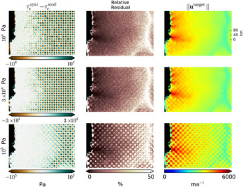
The improved resolution strength for faster flowing ice is in agreement with Gudmundsson (Reference Gudmundsson2003), who found that the transfer of basal topography and basal yield stress to the surface is highly dependent on the amount of motion at the base. Figures 10 and 11 show that the checkerboard pattern is transferred to the surface (visible in u
target) mainly for the fast-flow areas. An expression of the checkerboard pattern in u
target is only visible for the large amplitudes and wavelengths. And even in these extreme cases, the checkerboard pattern is not entirely recovered in $ \tau _{\rm c}^{\rm mod} $
.
$ \tau _{\rm c}^{\rm mod} $
.
The experiments performed in this section are a best case scenario, where the only source of uncertainty is introduced as noise in the surface velocity and the SSA is assumed to be valid for the entire drainage basin. Additional sources of error such as model or input parameter will most likely decrease the resolution strength further.
3.4. Initial conditions for Jakobshavn Isbræ
The limitations in resolution strength outlined in the last section exacerbate the problem that different solutions for the basal yield stress of the entire drainage basin are possible. The influences of prior estimate, ice softness, hybrid model, ice geometry, and gaps in data coverage are investigated with the experiments listed in Table 2 and results are shown in Figure 12. For all inversions the H 1 model norm is used in the regularization term and the regularization parameter is found with the L-curve method. The goal is to show sensitivities of the basal yield stress solutions and to suggest a basal yield stress field that should be used for prognostic model runs with the hybrid model of PISM. Therefore, most inversions in this section are performed with the hybrid model.
Sensitivity of real-data τ
c inversion to various choices. Real-data, drainage-basin-wide τ
c inversions for (1) constant $ \tau _{\rm c}^{\rm prior} $
, (2) temperature field from spin-up, (3) SSA only forward model, (4) temperature field and ice geometry from spin-up, (5)
$ \tau _{\rm c}^{\rm prior} $
, (2) temperature field from spin-up, (3) SSA only forward model, (4) temperature field and ice geometry from spin-up, (5) $ \tau _{\rm c}^{\rm prior} $
is set to the τ
c of the spin-up. The inversions are summarized in Table 2
$ \tau _{\rm c}^{\rm prior} $
is set to the τ
c of the spin-up. The inversions are summarized in Table 2

Inversion 1 uses a constant $ \tau _{\rm c}^{\rm prior} $
as a reference case for the following experiments. The value chosen for the constant is not important, as only its derivative enters the minimizing functional.
$ \tau _{\rm c}^{\rm prior} $
as a reference case for the following experiments. The value chosen for the constant is not important, as only its derivative enters the minimizing functional.
Inversion 2 was performed with a spatially-varying ice-temperature field from a constant-climate spin-up performed with PISM as outlined in Aschwanden and others (Reference Aschwanden, Adalgeirsdóttir and Khroulev2013). The general pattern of basal yield stress is similar to the constant ice softness experiment (Inversion 1), but the slow-flow area shows lower residuals compared with inversion 1. The constant ice softness used in inversion 1 was chosen to achieve an optimal fit in the terminus region, resulting in relatively soft ice. The ice softness from the spin-up on the other hand, indicates harder ice in the slow-flow areas. Therefore the ice velocities match the observations better even without introducing a stiff bed. In the fast-flow area, the basal yield stress patterns are very similar and differences are only visible north of Jakobshavn Isbræ. This justifies the choice of a constant ice softness for the area close to the terminus. However, for drainage-basin-wide inversions the changes in ice softness further upstream become important and improve the residuals greatly.
Inversion 3 matches observed surface velocities with velocities derived by the SSA only. The largest differences in modeled basal yield stress compared with the previous inversions occur in areas of slow-flow (low-resolution) and north of Jakobshavn Isbræ. The velocity residuals are lower than for the hybrid case and the residual patterns lack the wave-like features of the hybrid inversion.
Prognostic model runs need initial and boundary conditions for the entire model domain and spin-ups are used to produce a realistic and consistent temperature field within the ice. In the spin-up, the surface elevation of the ice is allowed to evolve and the surface at the end of the spin-up is also used as the initial state for prognostic runs. This surface elevation with the accompanying temperature field is used for inversion 4. Despite the use of the hybrid model in the inversion, the residuals do not display the wave-like features as seen in inversions 1 and 2. Using the hybrid model in the spin-up causes the surface to smooth out and the high driving stresses caused by the mismatch between surface elevation and bed topography are not present anymore. The hybrid inversion reduces the velocity residual when used with the ice geometry and temperature from a spin-up: only the fast-flow areas close to the termini still show large residuals. Note that the smaller outlet glaciers north of Jakobshavn Isbræ show the largest improvement in residual and a more realistic basal yield stress field compared with inversions with the observed ice surface elevation. In these outlet glaciers, the bed topography data are not as detailed as in Jakobshavn Isbræ and an evolved ice surface can compensate for these errors.
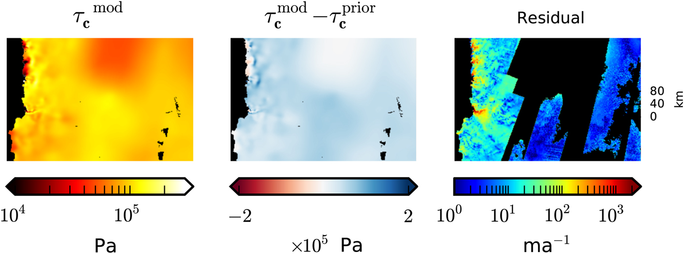
Inversion 5 uses the same ice geometry as inversion 4. Additionally, $ \tau _{\rm c}^{\rm prior} $
is set to the basal yield stress from the spin-up. In PISM, the basal yield stress is defined as the product between the tangent of a till friction angle and the effective pressure. The latter is calculated while the till friction angle has to be set heuristically. Here we follow the current implementation in PISM and define a linear relationship between the till friction angle and the bed elevation, assuming that lower till will be weak due to the existence of marine sediments. This definition results in a spatially varying τ
c that mirrors much of the small-scale structure found in the bed topography data, especially close to the terminus where radar efforts have led to a relatively detailed bed topography. The inferred
$ \tau _{\rm c}^{\rm prior} $
is set to the basal yield stress from the spin-up. In PISM, the basal yield stress is defined as the product between the tangent of a till friction angle and the effective pressure. The latter is calculated while the till friction angle has to be set heuristically. Here we follow the current implementation in PISM and define a linear relationship between the till friction angle and the bed elevation, assuming that lower till will be weak due to the existence of marine sediments. This definition results in a spatially varying τ
c that mirrors much of the small-scale structure found in the bed topography data, especially close to the terminus where radar efforts have led to a relatively detailed bed topography. The inferred $ \tau _{\rm c}^{\rm mod} $
shown in Figure 12 contains these small-scale structures because they do not affect the modeled velocities enough to be corrected. The difference between modeled and prior τ
c shows that a lowering of the basal yield stress is introduced in order to match the observed velocities. The residual field shows that a good match to observed velocities is easier when using a spatially constant value for
$ \tau _{\rm c}^{\rm mod} $
shown in Figure 12 contains these small-scale structures because they do not affect the modeled velocities enough to be corrected. The difference between modeled and prior τ
c shows that a lowering of the basal yield stress is introduced in order to match the observed velocities. The residual field shows that a good match to observed velocities is easier when using a spatially constant value for $ \tau _{\rm c}^{\rm prior} $
as done in inversion 4.
$ \tau _{\rm c}^{\rm prior} $
as done in inversion 4.
3.4.1. Data gaps
The influence of data gaps is investigated by excluding an area with missing data points from the misfit area. The misfit functional does not take into account grid points where data are missing, but the basal yield stress can still be corrected in these areas. We investigate various sizes of data gaps (Fig. 13) and find that large data gaps greatly influence the inferred basal yield stress. Smaller data gaps and those trending across the flow direction do not influence the inferred basal yield stress as strongly. Data gaps do not constrain the inverse method used here, but the basal yield stress solution for large areas with missing data will be strongly dependent on the prior estimate of basal yield stress.
Real-data, drainage-basin-wide τ c inversions with data gaps (blacked out areas shown in the right column) from the 2006 data set. Forward model, including ice geometry same as in experiment 4 (see Table 2).
4. DISCUSSION AND CONCLUSIONS
Synthetic experiments suggest that errors in surface velocity observations are not sufficient to explain the high residuals close to the terminus in real-data inversions. Errors in ice geometry lead to residual patterns that match the real-data inversion better, but only errors in the model are able to reproduce high residuals with similar patterns. This indicates that better forward models are needed in areas of complex flow, such as close to the terminus of Jakobshavn Isbræ. On the other hand, our residuals and relative residuals are comparable with the ones obtained by a full Greenland inversion with a Stokes model performed by Gillet-Chaulet and others (Reference Gillet-Chaulet2012). In their study, the regularization parameter was chosen for the entire ice sheet, not just for the drainage basin of Jakobshavn Isbræ as done in our study. Only a direct comparison of residuals from identical inversions could show how important the model simplifications are compared with the uncertainties in ice geometry. Other effects that are not incorporated in higher order models might also play a role, such as viscosity changes in older ice (Lüthi and others, Reference Lüthi, Funk, Iken, Truffer and Gogineni2002), ice softening due to water content in basal ice (Duval, Reference Duval1977) or ice crystal anisotropy (Horgan and others, Reference Horgan2008). This highlights the complexity of separating the different parameters and errors that are combined when doing inversions.
Checkerboard tests over the entire drainage basin show that for smaller amplitude and wavelength of perturbations the area where basal yield stress can be resolved is constrained to the fast-flow areas close to the termini. This effect is also apparent in the real-data inversions for the entire drainage area: the basal yield stress solution is highly dependent on the prior estimate in areas of low-resolution strength. Where the ice is frozen to the bed or basal motion is negligible, the observed surface velocities only contain information about the ice deformation and not the basal motion. Only when ice flow in these areas increases such that there is basal motion would we be able to make inferences about the properties at the base. These limitations in resolution lead to a high sensitivity of the inversion results to the initial estimate of basal yield stress.
The real-data inversions with the hybrid model display a small-scale wavy structure, which are particularly manifest in inversion 1 (Fig. 12). The higher residual points are caused by steep surface slopes, which lead to higher driving stresses for the calculation of the SIA component of the velocity. In many places, the calculated SIA velocities are indeed larger than the observed velocities leading to u target velocities that point in the opposite direction of the observed velocities. Therefore, the inversion algorithm is trying to match unrealistic velocity fields and is unable to achieve this, as seen in the large residuals. When using inversions to improve the initial boundary conditions at the base of the ice it is reasonable to perform the inversion with an ice geometry and temperature field from a spin-up; in this way a self-consistent model setup is achieved. Alternatively, inversions can be designed to simultaneously solve for basal topography and stresses (Raymond Pralong and Gudmundsson, Reference Raymond Pralong and Gudmundsson2011). It is also possible to use the basal yield stress at the end of the spin-up as the initial estimate in the inversion (Inv 6); so that only areas, where the velocity fields require a correction in τ c, will be adjusted. In this way, inconsistencies with the temperature field can be minimized; on the other hand, a lot of small-scale features are introduced with this type of initial estimate. As shown in Habermann and others (Reference Habermann, Truffer and Maxwell2013), such small-scale features in the prior estimate of basal yield stress will be preserved, especially when using a H 1 model norm.
Alternatively, recent works have focused on using mass continuity constraints to better define glacier beds (e.g. Morlighem and others, Reference Morlighem2011; McNabb and others, Reference McNabb2012; Brinkerhoff and others, Reference Brinkerhoff, Aschwanden and Truffer2016). A promising approach, not pursued here, would be to use such mass conservation methods to find basal topographies that are consistent with the forward model, while maintaining a measured surface elevation.
When using inversion algorithms it is important to define the questions and goals clearly. For realistic prognostic models of surface velocities the main goal might be to achieve a setup that is self-consistent while matching observations as closely as possible. For other studies, it might be more important to model the actual in situ basal yield stress as closely as possible. Different situations will make different modeling choices necessary. In all cases, it is important to remember the limitations of inverse results and that the resulting basal yield stress will incorporate other model errors, such as an incorrect temperature field.
In general, inverse methods are predicated on the minimization of a cost functional, which is just one scalar that represents misfit. However, the information in residual fields is considerably richer and should be used to help improve forward models or guide data acquisition. Jakobshavn Isbræ is a system undergoing rapid change; it is possible that some of the conclusions about error sources examined here do not generalize to other glaciers. However, the use of residual fields to guide further analysis should be generally applicable.
ACKNOWLEDGMENTS
This work was supported by NASA NNX09AJ38G, NSF CMG 0732602, NSF CMG 0724860, and in part by the College of Natural Science and Mathematics at the University of Alaska, Fairbanks. We acknowledge the use of data and data products from CReSIS generated with support from NSF grant ANT-0424589 and NASA grant NNX10AT68G. We thank Fabien Gillet-Chaulet for providing the Elmer/Ice run and for comments on the manuscript. Ed Bueler, Constantine Khroulev, and Andy Aschwanden have supported the modeling efforts and provided feedback. Frank Pattyn (Scientific Editor) and two anonymous reviewers provided valuable feedback. We would like to recognize the patience of the editorial team for the long delay during revision, while the authors were sorting out some modeling issues.


 Open access