

1. INTRODUCTION
Water storage in snow and ice is an important factor in the hydrological cycle in many regions of high altitudes and latitudes like Iceland, where 11% of the country is covered by glaciers (Bjornsson and Palsson, Reference Bjornsson and Palsson2008). Simulation and prediction of melt behavior provide valuable information for water resources management, e.g. regarding reservoir fill rates, potential power production and load on hydraulic structures. Short-term predictions of a few days improve daily operations and risk analysis, whereas longer term prediction of seasonal melt behavior assists in the systematic optimization of networks of reservoirs and diversions.
Prior work in melt modeling of Icelandic glaciers has focused on either empirical (degree day) and physical (energy balance) modeling approaches. Both have shown good performance for simulating glacial mass balance (e.g. De Ruyter de Wildt and others, Reference De Ruyter de Wildt, Oerlemans and Bjornsson2003b; Marshall and others, Reference Marshall, Bjornsson, Flowers and Clarke2005; Carenzo and others, Reference Carenzo, Pellicciotti, Rimkus and Burlando2009; Engelhardt and others, Reference Engelhardt, Schuler and Andreassen2014). Empirical approaches to mass-balance modeling have been considered sufficient when the underlying physical processes need not be resolved (e.g. Réveillet and others, Reference Réveillet, Vincent, Six and Rabatel2017). More recently, the vast potential of remote-sensing data has been increasingly applied to snowmelt estimation in basins where little information is available (Kalra and others, Reference Kalra, Ahmad and Nayak2013; Qiu and others, Reference Qiu, You, Qiao and Peng2014; Drolon and others, Reference Drolon, Maisongrande, Berthier, Swinnen and Huss2016).
Observations have shown that across the globe glaciers are losing mass and retreating. These studies have further concluded that the rapid retreat in the early 21st century is without precedent on a global scale (Barnett and others, Reference Barnett, Adam and Lettenmaier2005; Liu and others, Reference Liu2015; Zemp and others, Reference Zemp2015; Roe and others, Reference Roe, Baker and Herla2017). In line with the trend of glaciers globally, Icelandic glaciers have experienced retreat in recent years and their mass loss since the end of the 19th century has been shown to be responsible for 0.03 mm sea level rise globally (Bjornsson and others, Reference Bjornsson2013). Studies of the response of Icelandic glaciers to the expected climate change have shown that the country's main ice caps will mostly disappear over the next two centuries, leaving glaciers only at the highest elevations (Aðalgeirsdóttir and others, Reference Aðalgeirsdóttir, Johannesson, Bjornsson, Palsson and Sigurdsson2006, Reference Aðalgeirsdóttir2011).
Studies have predicted that increased glacial ablation will result in increased river runoff in Icelandic rivers throughout the 21st century (Jonsdóttir, Reference Jonsdóttir2010; Gudmundsson and others, Reference Gudmundsson2011; Matthews and others, Reference Matthews, Hodgkins, Gudmundsson, Palsson and Bjornsson2015). While little prior work exists on summer mass-balance modeling of Icelandic glaciers, several studies have considered the subject in other regions. These attempts have either employed statistical modeling techniques or used physical models forced with climate simulations (Fujita and Ageta, Reference Fujita and Ageta2000; Schöner and Böhm, Reference Schöner and Böhm2007).
The present study considers the prediction of the summer mass balance of Brúarjökull in SE Iceland. The Brúarjökull catchment, which is more than 90% glacierized, was harnessed for hydropower generation by the construction of the Halslon reservoir in 2006 (Gardarsson and Eliasson, Reference Gardarsson and Eliasson2006). Due to its hydroelectric potential, data have been recorded on hydro-meteorological variables in the catchment, including measurements of glacier mass balance since 1993 (De Ruyter de Wildt and others, Reference De Ruyter de Wildt, Klok and Oerlemans2003a, Reference De Ruyter de Wildt, Oerlemans and Bjornssonb; Rasmussen, Reference Rasmussen2005).
Brúarjökull covers an area of 1550 km2, making it the largest outlet glacier of the Vatnajökull ice cap, representing ~19% of the total area covered by the ice cap. The glacier ranges in elevation from 600 to ~1550 m a.s.l. and the mean equilibrium line lies at an altitude ~ 1200 m a.s.l. (Bjornsson and Palsson, Reference Bjornsson and Palsson2008). The glacier slopes gently toward the central Icelandic highland plateau and is classified as a surging outlet glacier with a surge frequency of 80–100 years, the last one occurring in 1964 (Kjær and others, Reference Kjær, Korsgaard and Schomacker2008). Unlike other outlets of the ice cap, Brúarjökull is not underlain by geothermal areas. Due to the proximity to surrounding volcanoes, its surface is periodically covered in volcanic tephra, thus decreasing its albedo (Larsen, Reference Larsen1998; Moller and others, Reference Moller2014). In the three main volcanoes near the basin, Bárðarbunga, Grímsvötn and Kverkfjöll, tephra events occur on average ~15 eruptions per century (Oladottir and others, Reference Oladottir, Larsen and Sigmarsson2011).
The forcing of physically based melt models with meteorological forecast model output on seasonal time scales inevitably incurs the large uncertainty in the forcing data. In this paper, statistical modeling was investigated to attempt the prediction of summer mass balance directly from the initial conditions of the system on the forecast date, thereby minimizing the uncertainties. The motivation for the study was to investigate whether the mass balance of the Brúarjökull could be predicted at the beginning of the melt season and to develop a simple operational model for reservoir operators. The goal of the study was to assess the predictive power of the information available by employing statistical approaches and the impact of lead times on predictions.
2. DATA
The data used in the present study consisted of glaciological mass-balance measurements, meteorological variables measured around the Brúarjökull basin, and climate indices which have been shown to correlate with Icelandic weather patterns (e.g. Baldwin and others, Reference Baldwin2003; Hanna and others, Reference Hanna, Jónsson and Box2004).
2.1. Glaciological measurements
Winter accumulation and summer ablation of Vatnajökull are measured in biannual measurement surveys at the boundaries of the melt season in spring and autumn. Winter accumulation is estimated by drilling ice cores and the summer ablation is measured from ablation wires or rods that are placed on the glacier in spring, when winter accumulation is measured (Thorsteinsson and others, Reference Thorsteinsson, Einarsson and Kjartansson2004). The annual net mass balance is calculated as the sum of the winter accumulation and the summer ablation. Figure 1 shows the approximate location of mass-balance sites on the surface of Brúarjökull as small circles.
Location of mass-balance points and automatic weather stations (AWS) which collect the meteorological data that were used in the study (Data on land cover from National Land Survey of Iceland).

The annual mass balance within each catchment on the glacier has been estimated based on the ablation stake measurements by extrapolating across the area (Palsson and others, Reference Palsson2014). The summer mass balance within the Halslon reservoir catchment was used as the response variable in the present study, while the winter accumulation at the various accumulation sites was used as an input variable. It should be noted that the estimated mass balance did not include liquid precipitation that fell on the glacier during the summer nor snow that melted outside the survey period. Furthermore, the uncertainty in the mass-balance measurements is not reported. The glaciological summer mass-balance data were selected as response variable based on the overlap of the shorter time series of discharge for the reservoir inflow which started in 2007.
2.2. Meteorological variables
Data were obtained from eight automatic weather stations (AWS) in and around the Brúarjökull basin. Three AWS on the glacier surface were used at elevations of 850, 1200 and 1400 m a.s.l. denoted as BruNe, BruMi and BruEf, respectively. The stations are designed to collect measurements of the components of the snow surface energy balance, shown as triangles in Figure 1. Time series of the measurements were acquired as daily averages of the following parameters: air temperature, relative humidity, net radiation, wind speed and surface albedo.
Data from ten land-based AWS surrounding the Brúarjökull basin were obtained, six based in the central highlands and four in the lowlands. The locations of the land-based AWS are shown as squares and pentagons in Figure 1. Time series were obtained as mean daily values of the following parameters: air temperature, dew point temperature, vapor pressure, relative humidity, atmospheric pressure and wind speed, and additionally precipitation measurements from the AWS at Egilsstadir.
2.3. Climatological variables
Icelandic climate has been shown to be significantly influenced by prevailing ocean conditions surrounding the island as well as changes in the large-scale circulations in the North Atlantic Ocean (Hanna and others, Reference Hanna, Jónsson and Box2001). Large-scale changes in atmospheric circulation have also been shown to correlate significantly with long-term Icelandic climate trends (e.g. Hanna and others, Reference Hanna, Jónsson and Box2004).
To incorporate information on the variability in the ocean conditions surrounding Iceland, the following two datasets were acquired: monthly averages of the Atlantic Multidecadal Oscillation (AMO) index (Enfield and others, Reference Enfield, Mestas-Nuñez and Trimble2001) and quarterly averages of the heat content of the Northern Atlantic (60–0°W, 30–65°N) measured in the top 700 m of the ocean by the US National Oceanic Data Center (NODC). The AMO index is defined from the trends in Sea Surface Temperature (SST) in the North Atlantic and has been shown to be correlated with temperature and precipitation patterns in Europe (Ghosh and others, Reference Ghosh, Müller, Baehr and Bader2017; Zampieri and others, Reference Zampieri, Toreti, Schindler, Scoccimarro and Gualdi2017). Furthermore, the heat transport through the North Atlantic by the warm Gulf Stream has been shown to be a key factor in determining the climate of Northern Europe (e.g. Palter, Reference Palter2015).
To incorporate information about the atmospheric circulations into the model, monthly averages of the North Atlantic Oscillation Index (NAOI) were acquired from the US National Oceanic and Atmospheric Administration (NOAA). The NAOI is a measure of the changes in the difference in atmospheric pressure at sea level between the Icelandic and the Azores. Studies have shown the NAOI to be significantly correlated with temperature and precipitation patterns in Iceland (Hanna and others, Reference Hanna, Jónsson and Box2004).
3. METHODS
3.1. Time series
The data were obtained as hourly or daily averages from the AWS and as point measurements of the winter accumulation data and climatological indices. The AWS data were aggregated to average values to represent the initial conditions of the system at four different dates in spring, specifically for the periods beginning on 1 April and ending on 15 May, 1 June, 15 June and 1 July.
The main aim of the study was to predict the summer inflow into the Hálslón Reservoir. Due to the short time series of inflow (2007–2015) the summer mass balance of Brúarjökull was selected as a proxy. Figure 2 shows the average daily discharge into the Halslon reservoir, where the shaded area shows the period between the forecast date on 1 July to the time of the fall ablation survey when the total summer mass balance of the glacier is calculated. The mass-balance data do not represent hydrological fluxes such as the drainage from the 10% of the basin, which is de-glacierized, baseflow and basal melt due to geothermal fluxes and liquid precipitation that falls on the glacier in summer. Despite this, we consider that the summer mass balance of the 90% glacierized portion of the basin offers a good representation of the inter-annual variability of net summer inflow into the reservoir. Thus, the total inflow, represented by the shaded area under the curve, will be significantly correlated to the summer mass balance, the quantity to be predicted in the present study.
Average daily discharge into Halslon reservoir for the period 2007–2015. The shaded area represents a proxy for the predicted mass balance.
The method was initially applied to 1 July data; then predictions of the summer mass balance were produced for each of the dates to assess the evolution of the predictive performance of the modeling approach in the period leading up to the summer melt season. The availability of the acquired data overlapped for the period 2001–2015, which was selected as the study period for the research. A breakdown of the input variables screened in the study along with their correlation to Brúarjökull summer mass balance is given in Appendix A.
The number of years used in the present study were N = 15. The input data were aggregated to a single average value for each year that represented the initial conditions of the system prior to the date of prediction. The data were split into training and test sets using the K-fold cross-validation method. In the present study, K was selected as 5 and the dataset was split into five subsets, each using three observations to test the model and 12 observations for calibration. A fivefold cross-validation was selected over a leave-one-out approach (where K = N) to reduce the variance in the error estimates (James and others, Reference James, Witten, Tibshirani and Hastie2013).
3.2. Variable selection
In the present study, many predictor variables were considered, whereas the number of observations of the response variable were few. To reduce the number of predictors and prevent model overfitting, variables were selected that showed a significant correlation with the response variable, the observed mass balance of the glacier. The variables were ranked by their r 2 value, and variables with r 2 values above a certain threshold were selected for further model development. The threshold value for variable selection was determined by sensitivity analysis of model results, as described in the subsequent sections.
3.3. Multivariate model ensemble
The selected variables can be used to create many multivariate regression models, none of which may be obviously superior to any of the others. Rather than selecting any single model, an ensemble of all potential competing models was developed. The selected variables were used to calculate a set of all possible multivariate linear regression models comprising five or fewer input variables. The input variables were limited to five due to computational limitations and the potential risk of overfitting the short time series. The optimal number of input parameters to include in the models of the ensemble was investigated by sensitivity analysis of model results with a range of numbers of input parameters, as described in subsequent sections.
3.4. Multi-model inference
Selection of any single one of the regression models in the set of possible models would recognize the existence of several potential and competing models and introduce additional uncertainty in the estimator due to the model selection. Unless the uncertainty associated with model selection is accounted for, overconfident estimates of model predictions may be inferred (Wang and others, Reference Wang, Zhang and Zou2009).
An alternative to selecting a single model is to average the prediction over a range of plausible models. This technique, called model averaging, incorporates the uncertainty associated with model selection into predictions of unknown variables (Hjort and Claeskens, Reference Hjort and Claeskens2003). The model averaging approach has in recent years been applied to several hydrological model applications (Diks and Vrugt, Reference Diks and Vrugt2010; Tsai, Reference Tsai2010).
Methods for model averaging include Bayesian model averaging (BMA) and frequentist model averaging (FMA). In BMA, model uncertainty is evaluated by assigning prior probabilities to all models being considered, whereas in the FMA, no prior probabilities are required and all estimators are determined by the data (Buckland and others, Reference Buckland, Burnham and Augustin1997; Raftery and others, Reference Raftery, Madigan and Hoeting1997; Hoeting and others, Reference Hoeting, Madigan, Raftery and Volinsky1999). In the present study, the FMA approach to model averaging was chosen as it relies only on the available data.
The response variable was estimated from a model ensemble by calculating the ensemble average. Several weighting functions have been reported in the literature to incorporate the measures of model plausibility into model averaging, based, for example, on goodness-of-fit metrics Akaike information criterion (Buckland and others, Reference Buckland, Burnham and Augustin1997), Bayesian information criterion and focused information criterion (FIC) (Burnham and Anderson, Reference Burnham and Anderson2002; Zhang and others, Reference Zhang, Wan and Zhou2012). Other strategies for weight function selection include the minimization of Mallow's C p criterion and weight choice based on the unbiased estimator of risk (Liang and others, Reference Liang, Zou, Wan and Zhang2011). In cases where little prior information is available on the likelihood of each model, or models having similar priors, assigning a uniform weight to each model is a reasonable choice (Raftery and others, Reference Raftery, Madigan and Hoeting1997). In the present study, a uniform weight was selected.
3.5. Optimal subset of models
Another important consideration of the model averaging methodology is the selection of a set of models over which to average. A complete Bayesian solution to the problem is to average over the entire set of possible models (Madigan and Raftery, Reference Madigan and Raftery1994). However, as the set of potential models can become large, averaging over the entire set may not be practical. To reduce the number of models to be considered, Madigan and Raftery (Reference Madigan and Raftery1994) suggested excluding models that poorly fit the calibration data.
The quality of each model in the set of possible models was assessed by several evaluation metrics. Moriasi and others (Reference Moriasi2007) surveyed several model evaluation metrics for watershed simulations and recommended using three metrics: the Nash–Sutcliffe efficiency (NSE), the ratio of the root mean square error to the std dev. of measured data (RSR) and the percent bias (PBIAS) for evaluation of hydrological models (Moriasi and others, Reference Moriasi2007). These three metrics were selected for model evaluation in the present study; their mathematical formulations are described as:
 $${\rm NSE} = 1 - \displaystyle{{\mathop \sum \nolimits_{i = 1}^n \left( {Y_i^{{\rm obs}} - Y_i^{{\rm sim}}} \right)^2} \over {\mathop \sum \nolimits_{i = 1}^n \left( {Y_i^{{\rm obs}} - Y^{{\rm mean}}} \right)^2}}, $$
 $${\rm RSR} = \displaystyle{{{\rm RMSE}} \over {{\rm STDEV}_{{\rm obs}}}} = \displaystyle{{\sqrt {\mathop \sum \nolimits_{i = 1}^n \left( {Y_i^{{\rm obs}} - Y_i^{{\rm sim}}} \right)^2}} \over {\sqrt {\mathop \sum \nolimits_{i = 1}^n \left( {Y_i^{{\rm obs}} - Y^{{\rm mean}}} \right)^2}}}, $$
 $${\rm PBIAS} = \displaystyle{{\mathop \sum \nolimits_{i = 1}^n \left( {Y_i^{{\rm obs}} - Y_i^{{\rm sim}}} \right) \times (100)} \over {\mathop \sum \nolimits_{i = 1}^n \left( {Y_i^{{\rm obs}}} \right)}},$$
where n is the number of data points in the dataset,  $Y_i^{{\rm obs}} $ is the observed mass balance in the ith year, $Y_i^{{\rm sim}} $ is the simulated mass balance in the ith year and Y mean is the mean observed mass balance. Moriasi and others (Reference Moriasi2007) suggested that a model simulation could be judged as satisfactory if NSE > 0.5, RSR < 0.7 and PBIAS < ±25%.
An ensemble of plausible models was created by evaluating all models in the set of possible multivariate regression models in accordance with the recommended values of NSE, RSR and PBIAS. Models with NSE < 0.5, RSR > 0.7 and PBIAS > ±25% were eliminated from further analysis and the remaining models were stored for multi-model inference.
Madigan and Raftery (Reference Madigan and Raftery1994) suggested that, in the case of models that fit the calibration data equally well, the less complicated model should be selected as it receives more support from the data. In the present study, a sensitivity analysis was performed on model predictions by varying the number of allowed input variables in the models and thus identifying the optimal number of variables to include.
The model averaging estimate of glacier ablation, Â, is then given by
 $$\hat A = \displaystyle{1 \over M}\mathop \sum \limits_{k = 1}^M \hat A_k, $$
where the index k denotes the kth model considered, M is the total number of models and  k is the estimated ablation based on the kth model. The uncertainty in the estimate is taken as the spread in predicted values of the ensemble of models.
4. RESULTS AND DISCUSSION
4.1. Multimodel inference
The selection of a threshold value of r 2 for variable selection and the number of input variables used in the model were optimized by performing a sensitivity analysis of the model results. The results were evaluated using the metrics NSE, RSR and PBIAS and were calculated using four threshold values of r 2 [0.2, 0.25, 0.3, 0.35] and five options for the number of model input variables [1, 2, 3, 4, 5]. Model ensembles were calculated for each combination of model options and the ensemble mean was used to calculate the evaluation metrics. The use of the median ensemble response was also investigated and yielded almost identical results. Tables 1–3 show the results for the evaluation metrics: NSE, RSR and PBIAS, respectively, while Table 4 shows the total number of models in each ensemble.
NSE of different model configurations with varying r 2threshold and number input variables, optimal value of NSE = 1

RSR of different model configurations, optimal value of RSR = 0

PBIAS of different model configurations, optimal value of PBIAS = 0

Number of models in the ensemble of plausible models with different configurations of number of input variables and threshold r 2 value

The results of the sensitivity analysis showed that the optimal values of NSE and RSR were obtained using a threshold value of r 2 = 0.3 and constraining the number of input parameters in the models to four (optimal results are highlighted in Tables 2–4). In terms of PBIAS, the optimal configuration was found with a threshold r 2 = 0.3 and two input variables in the models. However, the PBIAS of several configurations showed very low bias including the optimal configuration in terms of NSE and RSR. Hence it was concluded that the optimal model ensemble was achieved by selecting potential input variables with r 2 > 0.3 and restricting the number of inputs into each model in the ensemble to three. As shown in Table 4, this model ensemble contains 35 plausible models.
4.2. Variable selection
The time series of all the acquired potential input variables were assessed based on their correlation with the observed summer mass balance of Brúarjökull. Variables with a correlation coefficient below a set threshold value of 0.3 as determined in Section 4.1 were eliminated from further analysis. The variables selected for model development and their corresponding r 2 values are presented in Table 5.
Final variables selected for model development and their correlation to the observed summer mass balance of Brúarjökull, given as r 2 values

4.3. Model evaluation
The model was evaluated according to its ability to predict observed values of mass balance of the glacier in terms of the evaluation metrics NSE, RSR and PBIAS described in Section 3.5. The models were evaluated using fivefold cross-validation; thus, the data were split five ways providing 12 observations for calibration, leaving three observations for model evaluation for each fold. Table 5 shows the evaluation metrics obtained in the present study for each of the five folds used for cross-validation.
The results in Table 6 show that for four out of the five folds, all evaluation metrics indicated a satisfactory prediction in accordance with the specifications of Moriasi and others (Reference Moriasi2007). However, for the third fold, evaluated with observations from the period 2007–2009, low NSE and high RSR values were observed, whereas PBIAS was within acceptable range.
Evaluation metrics for model averaged predictions using fivefold cross-validation

Models show satisfactory performance with NSE > 0.5, RSR < 0.7 and PBIAS ⩽ ±25%.
Figure 3 shows the observed mass balance of the Brúarjökull for the study period with predicted values from each fold in a box and whiskers plot. The observed summer mass balance is shown as black stars; the notch in the box represents the median of the ensemble predictions, while the ends of the box represent the upper and lower quartiles; the whiskers encompass the range of all ensemble predictions. Considering the time series of simulated and observed values shown in Figure 3 during the period 2007–2009, both were very close to the long-term average mass balance of the glacier. When the observed values were close to the mean value, the denominator in Eqns (1) and (2) took on a small value, inflating the evaluation metrics, NSE and RSR. Thus, during periods where the mass balance is consistently close to the mean, these metrics may provide a poor indication of the quality of the model outputs.
Model averaged predictions of Brúarjökull summer mass balance for all fivefold cross-validations. Observed glacier mass balance is shown as black stars.
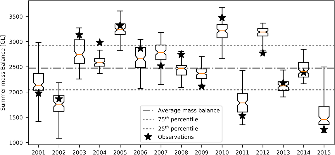
The results in Figure 3 show that the range of ensemble predictions encompasses the observed values for all observations in the study period except 2004 and 2012. Furthermore, the ensemble mean provides a reasonable estimate of the observed mass balance for the range of observations considered. The evaluation metrics described in Eqns (1)–(3) were calculated for all predictions yielding values of NSE = 0.71, RSR = 0.54 and PBIAS = 0.27%. The results suggest that the model has satisfactory performance with low bias for under- or overpredicting the mass balance.
4.4. Model performance in time
The results described in the previous sections were obtained using data available on 1 July. To assess how the predictive performance of the method evolved over time in spring, as the melt season approached predictions were calculated for data available for 15 May, 1 June and 15 June. Table 6 shows the evaluation metrics observed for predictions at each of these dates compared with 1 July.
The evaluation metrics presented in Table 7 show that the predictive information in the data diminished quickly as the lead time increased to dates prior to 1 July. For predictions made on 15 May, negative values of NSE were observed, indicating that the model predictions performed worse than simply reporting the mean mass balance of the glacier.
Evaluation metrics for predictions with longer lead times with models showing satisfactory performance on 1 July

Satisfactory performance is defined as models having NSE > 0.5, RSR < 0.7 and PBIAS ⩽ ±25%.
Figure 4 shows the predictions from the model suite using data from the four dates in spring. The results show that for longer lead times, the spread in ensemble predictions increased. Especially, ensembles for the years 2008 and 2009 showed a large variability in model outputs. The model also had poorer performance in predicting the extremes of the observations with longer lead times. The results show that predictions made prior to 1 July were less reliable and the earliest time when satisfactory predictions could be made was between 15 June and 1 July.
Model averaged predictions of Brúarjökull summer mass balance for all fivefold cross-validations. The optimal model found with 1 July data was forced with earlier data at three different dates between 15 May and 15 June.

Figure 5 shows the correlation of the selected input variables shown in Table 5 to the Brúarjökull summer mass balance at the four forecast dates in spring. The table shows that the key predictor on 1 July forecast, net radiation at BruNe, has much less predictive power earlier in the spring. The same applies to the albedo at both BruNe and BruMi, which show some predictive power on 15 June but none earlier. This suggests that spring snow conditions on the glacier are not indicative of the summer melt. By the end of June, as the melt season is beginning on the glacier, these variables start showing the power to predict the summer melt patterns.
Correlation of the selected predictor variables to Brúarjökull summer mass balance on four forecast dates in Spring.

The precipitation at Egilsstadir and atmospheric pressure at Karahnjukar similarly show little to no correlation to the summer mass balance on the earliest forecast dates. This suggests that the precipitation patterns in late spring and early summer play an important role in determining the summer melt, whereas precipitation patterns during the winter are less important in determining the ultimate summer melt. This can also be deduced from the fact that none of the winter accumulation measurements showed correlation to the observed summer mass balance.
The AMO index and the North Atlantic Ocean Heat content, however, show a persistent correlation to the summer mass balance throughout all the forecast dates. This suggests that a large portion of the inter-annual variability in Icelandic glacier mass balance is affected by the large-scale oceanic circulations and heat transport in the North Atlantic Ocean. The trends in these variables persist in much longer time frames than local climate conditions and contain significant predictive power for glacial mass-balance forecasts at least as early as the end of the first annual quarter. These results suggest that a significant portion of the variability in summer mass balance of Icelandic glaciers can be forecast well in advance of the melt season with lead times up to the length of the autocorrelative time scales of the AMO index.
Lastly, we note that the NAOI did not show any correlation to the summer mass balance. This suggests that large-scale atmospheric circulation in the North Atlantic, while indicative of Icelandic climate, is not an important factor in summer melt patterns of Icelandic glaciers. Hence, in terms of glacial mass balance, the ocean circulation in the North Atlantic is a much more important variable than atmospheric circulation.
5. CONCLUSION
The study showed that, of all the potential input variables available in the basin, seven showed a significant correlation with the summer mass balance. The variables deemed to contain predictive information at the beginning of the melt season were associated with average net radiation, glacier albedo, precipitation, atmospheric pressure and heat flux in the North Atlantic. It was observed that out of all potential multivariate regression models incorporating these variables, only a few adequately predicted summer mass balance. As selection of any single model would cause additional uncertainty in the estimation of the response variable due to model selection, an ensemble of plausible multivariate regression models was calculated and the average of the model results was used to predict the glacier mass balance.
The selection of a subset of plausible models over which to average was investigated. The results suggest that the optimal subset was found by eliminating models with poor fit to calibration data. Sensitivity analysis of model predictions suggested that the optimal number of input variables to include in the models was three and with variables exhibiting significant correlation included as inputs. The results showed that, in terms of the model evaluation measures NSE, RSR and PBIAS, satisfactory predictions of summer mass balance could be made by calculating a uniform average of model forecasts over the set of plausible models.
Investigation of the lead time with which predictions are calculated showed that model performance becomes less reliable as simulations are performed earlier in spring. Satisfactory predictions can be produced between 15 June and 1 July, at which time the melt season is beginning and predictions of summer melt volumes are valuable to water resources managers.
ACKNOWLEDGEMENTS
We thank the University of Iceland Research Fund which is supporting the first author. The project was also supported by the Energy Research Fund of the National Energy Company, Landsvirkjun by grants no. MEI-03-2015 and DOK-02-2017. We thank Landsvirkjun, the Icelandic Meteorological office and the Marine Research Institute for help with data gathering. We also thank Sverrir Gudmundsson and Finnur Palsson at the Institute of Natural Sciences at the University of Iceland, Oli Pall Geirsson at the Science Institute of the University of Iceland, Oli Gretar Blondal Sveinsson, executive VP for R&D at Landsvirkjun, and Ulfar Linnet, Manager of resources at Landsvirkjun, for numerous valuable suggestions to improve the paper.
APPENDIX A
See Table A1.
Breakdown of the potential input variables surveyed along with their correlation to Brúarjökull summer mass balance


 Open access