


1. INTRODUCTION
The concern that the Greenland ice sheet may experience a destabilising feedback between atmospheric temperature and ice velocity (Zwally and others, Reference Zwally2002; Parizek and Alley, Reference Parizek and Alley2004) has led to a concerted focus on the influence of surface melting on ice dynamics (Chu, Reference Chu2014). Observations indicate that the input of meltwater results in a net increase in ice velocity during the melt season (Zwally and others, Reference Zwally2002), but this effect is moderated by a subsequent drop in ice velocity to its annual minimum following the cessation of melting in the autumn (Sole and others, Reference Sole2013; Tedstone and others, Reference Tedstone2013). To explain these observations and assess their significance for the longer term stability of the ice sheet, it is necessary to understand in greater detail the mechanisms through which meltwater runoff influences ice motion. Much of our understanding of this topic is based on theoretical linkages between meltwater discharge, drainage system morphology and subglacial water pressure (Röthlisberger, Reference Röthlisberger1972; Kamb, Reference Kamb1987; Schoof, Reference Schoof2010), which have been applied to interpret recorded fluctuations in ice sheet motion during the melt season (e.g. Bartholomew and others, Reference Bartholomew2010; Hoffman and others, Reference Hoffman, Catania, Neumann, Andrews and Rumrill2011). Such explanations rely on an association of higher sliding velocities with higher basal water pressures (Bindschadler, Reference Bindschadler1983; Iken and Bindschadler, Reference Iken and Bindschadler1986), but how water pressure controls ice velocity remains poorly constrained (Sugiyama and Gudmundsson, Reference Sugiyama and Gudmundsson2004; Harper and others, Reference Harper, Humphrey, Pfeffer and Lazar2007). In order to better assess the potential future impact of increased melting on the dynamics of the Greenland ice sheet, it is therefore necessary to improve our understanding both of how meltwater discharge relates to basal water pressure, and how basal water pressure in turn relates to ice velocity.
The morphology of the subglacial drainage system is critical in determining how variations in meltwater input translate into variations in water pressure and ice velocity. The subglacial drainage system at alpine glaciers is traditionally divided into two main components, commonly termed distributed and channelized systems. Drainage through the distributed system is expected to occur in part through a network of linked cavities (particularly if the glacier is hard-bedded), which form in the lee of bumps at the ice/bed interface (Lliboutry, Reference Lliboutry1968). This process is inefficient, resulting in high basal water pressures and ice velocities when the onset of spring melt delivers additional runoff to the system. As surface melt increases during the spring, expansion of some of these drainage pathways leads to the formation of a network of subglacial channels (Nienow and others, Reference Nienow, Sharp and Willis1998). Drainage through these channels is far more efficient (Röthlisberger, Reference Röthlisberger1972), allowing large volumes to be discharged at relatively low water pressures, and causing ice velocity to drop (Kamb, Reference Kamb1987). These channels close when meltwater input is insufficient to offset closure through ice deformation, as is normally the case outside the summer melt season, and so the process repeats during the following melt season.
Observations from the ablation zone of the Greenland ice sheet suggest that the subglacial drainage system may undergo a similar seasonal evolution to that recorded at alpine glaciers (Bartholomew and others, Reference Bartholomew2011b; Chandler and others, Reference Chandler2013; Cowton and others, Reference Cowton2013). This model can go some way to explaining the observed characteristic seasonal ice velocity patterns, with highest velocities occurring early in the melt season when drainage pathways are least efficient (e.g. Bartholomew and others, Reference Bartholomew2011a; Sundal and others, Reference Sundal2011). However, more complete explanation of the observations requires a more detailed investigation of the processes connecting subglacial hydrology and ice dynamics. In particular, the interaction between channelized and distributed drainage systems remains relatively poorly understood. Tracing experiments suggest that ice velocities continue to exhibit significant variability in the presence of well-established subglacial channels (Chandler and others, Reference Chandler2013; Cowton and others, Reference Cowton2013), while observations suggest that water pressure fluctuations in subglacial channels exert a strong control on ice-sheet velocity on diurnal to multi-day timescales (Andrews and others, Reference Andrews2014). Because channels are expected to cover only a small fraction of the bed, any influence they exert over ice velocity must occur through interaction with the more widespread distributed drainage system (Hubbard and others, Reference Hubbard, Sharp, Willis, Nielsen and Smart1995; Nienow and others, Reference Nienow2005; Andrews and others, Reference Andrews2014). Understanding this connection is essential if the relationship between meltwater input and ice velocity is to be properly constrained.
More fundamentally, greater consideration is required as to why higher water pressures are associated with greater ice velocities. High water pressures permit the expansion of cavities across a wider area of the bed, allowing higher sliding velocities by reducing contact between the bed and the overlying ice (Lliboutry, Reference Lliboutry1968; Bindschadler, Reference Bindschadler1983). It has been argued that periods of highest ice velocity may however be driven by the process of cavity expansion, which exerts a down-glacier force on cavity walls (Iken, Reference Iken1981). Furthermore, the recognition of strong, short-term fluctuations in water pressure raises uncertainty as to how well cavity size and water pressure are in fact equilibrated at any time (Kamb and Engelhardt, Reference Kamb and Engelhardt1987; Howat and others, Reference Howat, Tulaczyk, Waddington and Bjornsson2008; Hewitt and others, Reference Hewitt, Schoof and Werder2012). These processes lie at the heart of sliding laws used in ice-sheet models to link water pressure and ice velocity (Bindschadler, Reference Bindschadler1983; Schoof, Reference Schoof2005). Addressing these uncertainties is therefore crucial if the effects of subglacial hydrology are to be realistically incorporated into ice-sheet models.
Recently, Andrews and others (Reference Andrews2014) used a combination of borehole pressure data and moulin water level records from a site in west Greenland to examine the effect of water pressure on ice motion. They argued that water pressure variations in the channelized drainage system, reflected in the moulin water level fluctuations, drove short-term, high-magnitude variations in ice velocity by reducing basal friction in adjacent unchannelized areas of the bed. We develop this concept by focussing on the mechanisms through which variability in water pressure, originating in subglacial channels and spreading to surrounding areas of the bed, drives variation in ice motion. To do so, we build on existing work undertaken at Leverett Glacier, a land-terminating outlet glacier in west Greenland. In particular, Bartholomew and others (Reference Bartholomew2012) used modelled subglacial water pressures and high-resolution ice velocity records to demonstrate the importance of variability in meltwater input with respect to ice dynamics. We continue this theme by examining in detail the relationship between horizontal and vertical ice motion at this site. Because the vertical motion of the ice surface in part reflects the volume of basally stored water, this provides insight into cavity expansion and contraction and its influence on ice dynamics (e.g. Iken and others, Reference Iken, Röthlisberger, Flotron and Haeberli1983; Sugiyama and Gudmundsson, Reference Sugiyama and Gudmundsson2004). Specifically, we seek to test Iken's (Reference Iken1981) hypothesis that ice motion is more sensitive to the rate of change of cavity volume than absolute cavity volume, and assess the implications of this for the dynamics (and modelling of the dynamics) of the Greenland ice sheet. These data are then analysed in conjunction with time series of subglacial channel water pressure, derived through a combination of moulin water-level measurements and hydrological modelling, to assess how variation in meltwater input to this outlet glacier translates into variation in water pressure and ultimately ice motion.
2. METHODS
2.1. Study site
Leverett Glacier is a land-terminating outlet glacier in west Greenland (Fig. 1), with an estimated hydrological catchment of >600 km2 (Bartholomew and others, Reference Bartholomew2011b; Palmer and others, Reference Palmer, Shepherd, Nienow and Joughin2011). The glacier was subject to a program of hydrological and glaciological investigations during 2008–2012 – this study focuses on data from 2010, when instrumentation of the lower part of glacier was most complete. Initial examination of ice dynamics and proglacial hydrology demonstrated a seasonal increase in subglacial drainage efficiency beneath the ablation zone of this sector of the ice sheet (Bartholomew and others, Reference Bartholomew2010, Reference Bartholomew2011a, Reference Bartholomewb). This hypothesis was supported by tracer investigations, which indicated that channels form quickly beneath Leverett Glacier each spring and extend to at least 40 km inland from the ice margin (Chandler and others, Reference Chandler2013; Cowton and others, Reference Cowton2013). Subsequent studies have demonstrated that while increasing melt input can trigger periods of significantly elevated ice velocity over periods of hours to days (Bartholomew and others, Reference Bartholomew2012), these speed-up events have negligible impact on ice velocities on inter-seasonal timescales (Sole and others, Reference Sole2013; Tedstone and others, Reference Tedstone2013).
(a) Map showing the estimated hydrological catchment of Leverett Glacier (dark grey shading; Bartholomew and others, Reference Bartholomew2011b; Palmer and others, Reference Palmer, Shepherd, Nienow and Joughin2011; Cowton and others, Reference Cowton, Nienow, Bartholomew, Sole and Mair2012) on the western margin of the Greenland ice sheet (pale grey shading), with ice surface contours (m) from a DEM derived from InSAR (Palmer and others, Reference Palmer, Shepherd, Nienow and Joughin2011). The white rectangle denotes the area expanded in the subset map, (b). Also shown are GPS locations S1–S6 (stars) and the airborne geophysical transect (black line; Allen, Reference Allen2010; Krabill, Reference Krabill2010), from which the profiles of ice surface and bed elevation are derived, (c). (b) Landsat ETM+ image of the lower section of Leverett Glacier, showing ice surface contours (m) (white), GPS site S2 (star), moulins L4 and L7 (circles), the gauging site (triangle) and the approximate inferred location of a major subglacial channel (dashed black line; Cowton and others, Reference Cowton2013). (c) Profiles of ice surface (black) and bed (grey) elevation along the airborne geophysical transect (a), showing the locations of GPS sites S1–S7 (stars).

2.2. Ice velocity
Ice surface velocity was monitored through the 2010 melt season at seven sites (S1–7) located along a transect extending between ~2 km and 115 km from the glacier terminus (Fig. 1). At each site, a dual-frequency Leica 500 or 1200 Series GPS receiver was mounted onto a pole that was drilled into the ice-sheet surface and subsequently frozen in place. These data were processed to give horizontal and vertical ice positions, and subsequently velocities, as described by Bartholomew and others (Reference Bartholomew2012). Errors in the horizontal and vertical position are estimated to be ±0.005 and ±0.01 m, respectively (Bartholomew and others, Reference Bartholomew2011a). These positions are differenced across a 6 h moving window to generate velocities, resulting in uncertainties in horizontal and vertical velocity of ±0.04 and ±0.08 m d−1, respectively (Bartholomew and others, Reference Bartholomew2011a). Typical horizontal velocities are in the range 0.1–1 m d−1, but variation in the vertical position of the GPS units is much smaller (<0.1 m d−1), meaning much of the vertical position signal lies close to the accuracy limit of the data (Fig. 2). A particular problem results from multipath effects (e.g. Larson and others, Reference Larson, Bilich and Axelrad2007), which generate spurious periodic signals with a frequency of one sidereal day (~23:56) and harmonics thereof. To minimize these errors, the vertical position data were decomposed using a Fourier transform, allowing the spurious signals at these known frequencies to be removed before transforming the data back into the time domain. Following this, the data were subject to quality checks, discarding days for which the records were exceptionally noisy (std dev. >0.04 m) or patchy (>20% of data points missing). The data were then smoothed using a phase-preserving filter over a 24 h window, leaving only the more robust day-to-day variability in vertical position. The 24 h mean velocities were calculated over a window from 0700 to 0700 h the following day, typically covering the period from one diurnal horizontal velocity minimum to the next.
Motion of the GPS units S1–3 and S5–7 during the 2010 melt season, shown prior to the filtering as described in Section 2.2, and the trend removed at each site to reveal vertical motion due to bed separation (uplift). At S5–S7, the pre-melt season data from which these trends were calculated are shown in black. The transition from ‘Pre-melt’ to ‘During melt’ occurs on 2 June (S4), 10 June (S5) and 6 July (S7). At S1–S3 the trends were calculated based on data from 2009 (Section 2.2.). All positions are shown relative to the position of the units at the start of the time series on 25 April.

Because the GPS receivers are mounted on fixed poles, the recorded vertical movement is independent of ablation. The signal instead comprises a combination of the vertical component of along-flow motion, longitudinal strain and uplift due to varying volumes of basal water storage (Iken and others, Reference Iken, Röthlisberger, Flotron and Haeberli1983; Sugiyama and Gudmundsson, Reference Sugiyama and Gudmundsson2004). To remove the vertical component of along-flow ice motion, the vertical position was detrended with respect to the horizontal position by subtracting the trend apparent prior to the onset of melting in the spring (Fig. 2). At the lower three sites (S1–S3) the early onset of melt in 2010 limited the time available to ascertain this trend. Comparison of the pre-melt season trends at S5–7 in 2010 with those from the same sites in 2009, when a longer record was obtained prior to the onset of melting (Bartholomew and others, Reference Bartholomew2011a), revealed very similar trends between years at the individual sites. As such, detrending at S1–3 was undertaken based on data from S1 to 3 during spring 2009, when pre-melt season ice motion was recorded at these sites. The gradient of the removed trend is positive at the lower sites (i.e. there is a net upward movement), transitioning to negative at the upper sites (Fig. 2), a trend which likely reflects the average bed slope in these regions (Fig. 1). This detrending procedure will also remove any extension or compression that is proportional to horizontal motion – for example, the compression that would occur as ice is funnelled through a narrowing in the glacier. The remaining signal should therefore contain only the uplift and the longitudinal strain occurring due to local variations in ice velocity. Seismic data suggest there may be areas of subglacial sediment in the vicinity of Leverett Glacier (Dow and others, Reference Dow2013), and as such the uplift signal may reflect the dilation of subglacial till as well as the storage of water in subglacial cavities. The effects of these processes are difficult to separate in the ice motion data. The maximum uplift due to till dilation is however limited by the porosity of till and the depth to which water pressure fluctuations can penetrate into the till layer, and thus is expected to be small compared with uplift due to cavity formation (Howat and others, Reference Howat, Tulaczyk, Waddington and Bjornsson2008).
2.3. Water pressure
2.3.1 Recorded moulin water level
We used HOBO pressure transducers to monitor ponded water levels in two moulins (termed L4 and L7; Fig. 1) during the 2010 melt season, with the objective of obtaining a measure of water pressure in the subglacial drainage system in the vicinity of GPS site S2 (Cowton and others, Reference Cowton2013). The pressure transducers were suspended into the moulins on fixed lengths of cord; however, this alone does not give the depth of the sensor below the surface as the moulin may not descend vertically into the ice. At L4, the depth of the sensor below the surface was confirmed by the recorded distance between the glacier surface and the pooled water at a time when this was sufficiently close to measure manually (which occurred during a visit to the site on 29 May). This opportunity did not arise at L7. Instead, the depth of the sensor below the surface is constrained between a maximum value (known from the length of cord to which it was attached) and a minimum value (calculated from the recorded depth of pooled water above the sensor, which cannot exceed the ice surface).
The bed elevation at L4 and L7 is obtained from a NASA IceBridge ice penetrating radar flightline (Allen, Reference Allen2010), which passes within 500 m of both moulins (Fig. 1). We assume that the ponded water represents the upper part of a column of water extending to the bed, and as such the height of the column can be interpreted as equivalent to the pressure head at the bed. Furthermore, it is expected that as a point of concentrated meltwater input, moulins will connect to the channelized subglacial drainage system (Andrews and others, Reference Andrews2014), a hypothesis supported by dye-tracing experiments at these moulins during the 2010 melt season (Cowton and others, Reference Cowton2013). We therefore assume that moulin water levels will be indicative of water pressure in subglacial channels, something which is difficult to obtain using boreholes due to the small proportion of the bed that such channels occupy (Fountain and Walder, Reference Fountain and Walder1998). Unfortunately, the water level records from both moulins are limited by their short duration (the sensors at L4 and L7 were deployed on 25 and 31 May and ceased functioning on 3 and 9 June, respectively), and also by the tendency of the water level to drop below that of the sensor.
2.3.2 Modelled water pressure
Because of the difficulties in obtaining water pressure measurements, we supplement the short moulin dataset by modelling water pressure in the vicinity of S2. Bartholomew and others (Reference Bartholomew2012) used a simple hydrological model to simulate variation in water pressure associated with fluctuations in meltwater input to a moulin at this site. Their model was forced entirely by local melt inputs, which entered a moulin connected directly to the ice margin by a channel. A more likely scenario, however, is that drainage from the moulin connects with a major tributary channel draining the large catchment upstream of this site (e.g. Schoof, Reference Schoof2010). In this way, local pressure variations will reflect surface meltwater input both locally and further upstream (e.g. Nienow and others, Reference Nienow, Sharp and Willis1996).
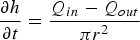
To represent this system, we use a simple, two component set up, comprising the subglacial trunk channel and a short tributary channel (Fig. 3; Table 1). In this way, the response of water pressure to both catchment-scale (i.e. trunk) and local (i.e. tributary) changes in meltwater input can be incorporated. The set up of the tributary resembles that of Bartholomew and others (Reference Bartholomew2012). Supraglacial runoff Q in enters a moulin represented by a cylindrical shaft of radius r. Water level (i.e. pressure head) h in the moulin varies according to
 $$\displaystyle{{\partial h} \over {\partial t}} = \displaystyle{{Q_{in} - Q_{out}} \over {\pi r^2}}$$
where Q out is equal to the discharge along the tributary channel. Discharge Q along a semi-circular channel is given through the Darcy–Weisbach law
 $$Q = c_3S^{5/2}\left \vert {\rm \Psi} \right \vert ^{ - 1/2}{\rm \Psi} $$
where S is channel cross section and $c_3 = {{2^{1/4}\sqrt {\pi + 2}} / {(\pi ^{1/4}\sqrt {\rho _{\rm w}f} )}}$
, ρ
w is the density of water and f is a friction factor (constants c
1–3 are named for consistency with Schoof, Reference Schoof2010). The hydraulic gradient Ψ along the tributary is
$c_3 = {{2^{1/4}\sqrt {\pi + 2}} / {(\pi ^{1/4}\sqrt {\rho _{\rm w}f} )}}$
, ρ
w is the density of water and f is a friction factor (constants c
1–3 are named for consistency with Schoof, Reference Schoof2010). The hydraulic gradient Ψ along the tributary is
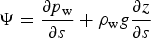 $${\rm \Psi} = \displaystyle{{\partial p_{\rm w}} \over {\partial s}} + \rho _{\rm w}g\displaystyle{{\partial z} \over {\partial s}}$$
where s is along channel distance, z is bed elevation and g is gravitational acceleration. Water pressure p w at the head of the tributary channel is determined by the pressure head in the moulin through p w = ρ w gh, while that at the downstream end is determined by the pressure of the trunk channel. The evolution of S is subsequently calculated according to
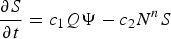 $$\displaystyle{{\partial S} \over {\partial t}} = c_1Q\Psi - c_2N^nS$$
Schematic depicting the configuration of the hydrological model.

Symbols and parameter values

Values of flow law parameter A used in the three scenarios. For each scenario, the correlation coefficient R is shown for 12 h intervals (coinciding approximately with the daily minima and maxima), 24 h mean values and 24 h mean values using the modelled steady-state water pressure (dashed curves in Fig. 8). Correlations include all data from 24 May onwards (i.e. the period of unphysically high pressures immediately following the onset of runoff is not included)

All values are significant at p-value < 0.01.
(Schoof, Reference Schoof2010). The first term on the right-hand side of Eqn (4) is the rate of channel opening due to wall melting, with c 1 = 1/ρ i L where L is the latent heat of fusion per unit mass of ice and ρ i is the density of ice. The second term is the rate of channel closure due to viscous creep, where N = p i − p w is effective pressure (p i is ice overburden pressure) and c 2 = 2An −n . A and n are parameters from Glen's flow law determining ice rheology, typically taken as n = 3 and A = 2.4 × 10⁻²⁴ Pa−3 s−1 for clean temperate ice (Cuffey and Paterson, Reference Cuffey and Paterson2010; Schoof, Reference Schoof2010). Assigning a value to the flow law parameter A remains difficult however, with the value varying by several orders of magnitude depending on poorly constrained physical properties of the basal ice (Hooke, Reference Hooke2005; Cuffey and Paterson, Reference Cuffey and Paterson2010). As such, while the initial simulation of channel evolution was undertaken using the values specified above, additional experiments were undertaken using a range of values for the flow law parameter A in order to examine the impact of basal ice rheology on modelled water pressures (Table 2).
To model the trunk channel in a similar way would require accounting for the distributed input of meltwater across the catchment. Much simpler is to use the discharge of meltwater exiting the channel at the ice margin, which was monitored at a site ~2 km from the ice margin (as described by Bartholomew and others (Reference Bartholomew2011b)). Given the vast size of the catchment upstream of S2 (>600 km2 relative to ~15 km2 between S2 and the margin), it is reasonable to assume that the relative change in discharge between S2 and the margin is negligible (Fig. 1). Furthermore, it is likely that the majority of this water travels in a single trunk channel draining from the upper catchment (an assumption supported by the presence of an obvious trough in the ice surface along the lowermost 2 km of the glacier). In this case, Eqn (2) can be rearranged to give the pressure gradient required to give the recorded proglacial discharge:
 $${\rm \Psi} = \displaystyle{{Q^2} \over {c_3^2 S^{5/2}}}.$$
Because at the ice margin the elevation is known and the channel is unpressurized, Eqn (3) can then be solved for water pressure in the trunk channel in the vicinity of S2.
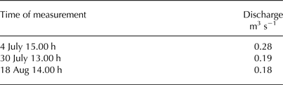
For simplicity, the pressure in the trunk is considered to be independent of the tributary channel. As such, coupling between the two channels is one way, with pressure in the trunk influencing the gradient along the tributary channel. The model is run using an Eulerian time step of 10 s, and is initiated at the onset of the melt season using a stable channel size based on a trunk discharge of 1 m3 s−1 and a tributary discharge of 0.01 m3 s−1. Supraglacial input to the moulin is based on melt records obtained using an ultrasonic distance gauge (UDG) fixed at S3, located 10 km east of S2 (Fig. 4). This method provides an accurate, high resolution measure of ablation that can resolve diurnal melt cycles more accurately than a positive degree-day melt model (which will not work well at high temporal resolution; Hock, Reference Hock2003). This is critical if diurnal pressure fluctuations are to be reproduced. Snow depth at S2 and S3 was only ~3 cm at the onset of the melt season, hence no attempt is made to differentiate between the meltwater contribution of snow and ice melt. Melt rates are used to calculate runoff from a supraglacial catchment area of 1 km2. This catchment area was chosen such that peak melt input to the moulin was ~0.1–0.5 m3 s−1, in keeping with three measurements of supraglacial input at L7 based on supraglacial channel cross section and velocity (Table 3). The modelled subglacial water pressures are sensitive to the relative variability in meltwater input rather than the absolute volume of meltwater input, and so are not sensitive to errors in estimation of supraglacial catchment area (doubling or halving the catchment area changes the mean modelled moulin water level by <1%). Unfortunately, the UDG failed on 14 June. Thus, while trunk pressure is calculated throughout the melt season, moulin water level is only calculated until this date. Nevertheless, this time frame overlaps with the observations of moulin water level, facilitating comparison of the modelled with recorded water levels.
Melt rate obtained from the UDG at S3 (left axis), scaled to give runoff used as input to the moulin in the hydrological model (right axis).

Measurements of supraglacial melt water input at moulin L7
The hydrological model used here contains many simplifications – there is no evolution between distributed and channelized drainage, only two branches of the drainage network are considered and pressure is assumed to change linearly along these branches. It is thus much less sophisticated than the present state-of-the-art in glacial hydrological modelling (e.g. Hewitt and others, Reference Hewitt, Schoof and Werder2012; Schoof and others, Reference Schoof, Hewitt and Werder2012; Werder and others, Reference Werder, Hewitt, Schoof and Flowers2013). However, the present set up is intended to best utilize the existing hydrological (proglacial discharge and moulin water level) and ice velocity data to explore the relationship between meltwater discharge, water pressure and ice motion.
3. RESULTS
3.1. Ice velocity
Horizontal ice velocity u and detrended vertical ice velocity w are shown through the 2010 melt season at each site in Figure 5. There are gaps in the data due to technical issues (most often a loss of power) – in particular, S4 failed early in the season and is not shown (or discussed further), while S5 ceased recording at the start of August. With the exception of S7, ice motion during the summer months is punctuated by a series of spikes in u, concentrated earlier in the season at sites closer to the margin (Fig. 5). These events are generally coincident with periods of increasing runoff due to increasing melt rates or lake drainage events (Fig. 5g) (Bartholomew and others, Reference Bartholomew2011a; Tedstone and others, Reference Tedstone2013). The detrended vertical position of the ice surface typically increases during the early part of the melt season, before declining again during the latter part, often to a level below its start position in the spring. However, what is particularly striking is the similarity between the horizontal and vertical velocity records (Figs 5, 6a; Table 4). This correlation exists for all sites except for the uppermost site where u remains almost constant.
(a–f) The 24 h mean values of horizontal ice velocity u, vertical ice velocity w and detrended ice surface elevation z (expressed relative to the pre-melt season elevation on 25 April) during the 2010 melt season. Pale colours show periods during which the vertical position data did not pass quality checks (Section 2.2) – these sections are linearly interpolated for ease of visualization, but are not used in analysis. Also shown in (b) is 24 h mean modelled channel water pressure, expressed as a fraction of ice overburden pressure. (g) Proglacial discharge during the same period. Shading denotes periods of enhanced horizontal velocity at least one site.

(a) Horizontal and vertical ice velocity over 24 h windows. Horizontal velocity is shown minus the average pre-melt season ‘background’ horizontal velocity at each site, hence negative values indicate periods when ice velocity was lower than this pre-melt season value. Vertical velocity is calculated from the detrended GPS records, as described in Section 2.2. Coloured dots denote data from different sites. The black line shows the best fit for all sites for days with vertical velocity >0 m d−1, with the extrapolation of this trend shown by the dotted line. (b) As for (a), except showing mean detrended vertical position z (relative to the pre-melt season position) rather than vertical velocity on each day. Correlation coefficients are given in Table 4.

Correlation coefficient (R) values between vertical and horizontal motion (Fig. 6)
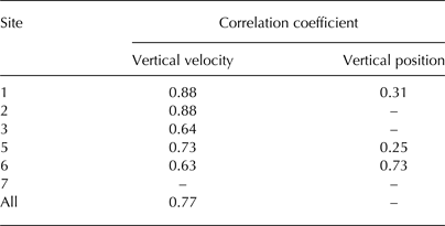
R values for vertical velocity are for all days when vertical movement is positive (upward), while those with respect to vertical position are for all data. All values shown are significant at p-value < 0.01.
Before these features can be further explored, it is necessary to rule out, as best as possible, strain due to local velocity variations as an explanation for the recorded vertical motion (Sugiyama and Gudmundsson, Reference Sugiyama and Gudmundsson2004). Because the GPS records are detrended with respect to horizontal ice motion, this process should remove compression/extension that is topographically determined and so scales with ice flow velocity. This leaves strain occurring due to local acceleration or deceleration of a region relative to ice up- or down-glacier of that location. An example of this can likely be seen at S7 during the later summer, where gradual thinning is interpreted as stretching in response to acceleration in the region of S6 (Figs 2f, 5f). Calculating strain due to longitudinal coupling is difficult in any setting, and especially at Leverett Glacier due to the unconstrained lateral margins of the catchment and wide spacing of the GPS units. Studies at alpine glaciers that have attempted to calculate temporal variability in vertical strain have however found it to be smaller than and typically of opposite sign to periods of uplift recorded at times of high horizontal velocity (Iken and others, Reference Iken, Röthlisberger, Flotron and Haeberli1983; Anderson and others, Reference Anderson2004). As such, while we recognize that this signal may influence the patterns we observe, we follow many previous studies (e.g. Iken and others, Reference Iken, Röthlisberger, Flotron and Haeberli1983; Anderson and others, Reference Anderson2004; Howat and others, Reference Howat, Tulaczyk, Waddington and Bjornsson2008; Bartholomew and others, Reference Bartholomew2011a; Hoffman and others, Reference Hoffman, Catania, Neumann, Andrews and Rumrill2011) in attributing vertical motion in the detrended records principally to uplift due to variability in water storage at the bed.
3.2. Water pressure
Moulin water levels fluctuated strongly over diurnal cycles during the observation period (Fig. 7a). Diurnal peaks in water pressure often exceeded ice overburden, with the level of pooled water at L4 reaching the ice surface on atleast two occasions. The relative magnitude of the spikes in water level recorded at the two moulins reflects in part the depth of the pressure transducer below the ice surface, as the lower range of the water level fluctuations are lost below the levels of the sensors. At L4, where a greater part of the pressure cycle was captured, these fluctuations exceeded 40 m (~20% of ice overburden). Both moulins also demonstrated day-to-day variations in maximum water level, albeit smaller than the variation observed over diurnal cycles. At L4, maximum recorded water level rose steadily from 26 to 31 May, then declined slightly before the record was lost. Only one daily water level minimum was recorded, on the morning of 26 May, when water level at L4 fell to ~93% of overburden. Water level dropped consistently below this during subsequent nights, but the minimum values reached are unknown as they occurred below the level of the sensor.
(a) Recorded moulin water pressure at L4 and L7, expressed as a fraction of ice overburden pressure. At L7 the exact depth of the sensor below the surface could not be ascertained, and so the range of possible values is shown (Section 2.3.1). (b) Modelled trunk (dashed) and moulin (solid) water pressures, expressed as a fraction of ice overburden pressure. Three sets of modelled water pressures are shown, reflecting the parameter combinations given as Scenarios 1–3 in Table 2. (c) Recorded horizontal velocity and detrended vertical position and velocity at S2 over the same time span.

Modelled water pressures follow the same trends as moulin water levels during the short period in which these observations exist (Fig. 7b). Peak daily water pressures rise steadily throughout the last days of May before dropping again, while the predicted spike in water pressure on 5 June is recorded as a period of high water level at L7. The modelled trunk and moulin water pressures are well equilibrated at night, when local supraglacial inputs are often absent. During the day however, modelled moulin water pressures rise much higher than trunk channel water pressures. The magnitude of these fluctuations reflects the degree of variability in discharge through the tributary and trunk channels. Because the local meltwater input to the tributary fluctuates greatly over diurnal cycles, the channel cross section is poorly adjusted to discharge at any time and pressure may depart significantly from the steady-state value (as reflected in the results of Bartholomew and others (Reference Bartholomew2012), who used only the local melt input to model water pressure). Discharge in the trunk channel (as evidenced by the proglacial discharge; Fig. 5g) varies comparatively little over diurnal cycles because it reflects the integration of numerous water sources over a large catchment (Bartholomew and others, Reference Bartholomew2011b). As such, the channel cross section remains relatively well adjusted and the pressure fluctuations are smaller (Fig. 8). The effect of varying the flow law parameter A is discussed in the following section (Section 4.1).
In addition to the main water pressure time series in Figure 8, additional time series are given showing the steady-state pressure for the mean discharge on each day (dotted curves). This eliminates the transient fluctuations in pressure associated with short-term variations in discharge, allowing the significance of the variation in steady-state water pressure with channel size to be evaluated. It is recognized that pressure drops as discharge rises in channels in steady state (Röthlisberger, Reference Röthlisberger1972); however, the simulated steady pressures vary little relative to the transient fluctuations, declining by <5% between the early melt season (when the discharge is ~10 m3 s−1) and the height of the melt season (when the discharge is ~400 m3 s−1), suggesting this effect is not of primary importance as a control on water pressure and ice dynamics.
(a) Modelled trunk water pressure at S2, based on the parameter values given in Table 2. The dot-dashed line shows ice overburden pressure. Dotted curves show the steady-state pressure for the mean discharge on that day for each scenario. (b) Trunk channel cross-sectional area under the same three scenarios.

4. INTERPRETATION
4.1. Modelled water pressure
The agreement between the modelled and observed moulin water pressures is improved in the softer ice (i.e. higher A) scenarios (Scenario 2–3, Table 2; Fig. 7b). Softer ice increases the water pressure by increasing the rate at which the channel can close through ice deformation (Eqn (4)). This means that in the softer ice scenarios, the balance between channel opening and closing is found at a higher water pressure (lower effective pressure), as this serves to reduce the rate of creep closure and increase the rate of wall melting (in the latter case, by raising the hydraulic gradient and hence channel flow velocities). The finding that the agreement between modelled and observed water pressure is improved using values of A >2.4 × 10⁻²⁴ Pa3 s−1 is not unexpected – for example, both Röthlisberger (Reference Röthlisberger1972) and Iken and Bindschadler (Reference Iken and Bindschadler1986) found a better match between observations and model results using values of A of order 10−23 Pa3 s−1 (similar to Scenario 2, Table 2). Basal ice may indeed be relatively soft due to the increased presence of impurities (Iken and Bindschadler, Reference Iken and Bindschadler1986; Cuffey and Paterson, Reference Cuffey and Paterson2010), and particularly so in Greenland due to the presence of softer Weichselian/Wisconsinan ice in the lower layers of the ice sheet (Ahlstrom and others, Reference Ahlstrom, Mohr, Reeh, Christensen and Hooke2005; Colgan and others, Reference Colgan2011). Furthermore, it has been argued that subglacial channels are characteristically low and broad rather than semicircular in cross section (Hooke and others, Reference Hooke, Laumann and Kohler1990). This alternative form would increase both the rate of creep closure and the channel roughness, increasing the water pressure required to maintain equilibrium at a given discharge.
Nevertheless, it is not clear whether the value of A of 10−22 Pa3 s−1 used in the softest ice scenario (Scenario 3, Table 2) is physically justified. There is some precedent for values of this magnitude, with Nye (Reference Nye1953) requiring A = 1.4 × 10⁻²² Pa3 s−1 to match recorded tunnel closure rates at the Haut Glacier d'Arolla, Switzerland. In this case, the high closure rates were attributed to a zone of high compressive stress, an explanation that may be appropriate here due to the reverse bed slope in the region of L4 (Fig. 1). In addition, the under-prediction of diurnal moulin water level spikes by the model may simply reflect an overestimation of local drainage system efficiency at this time. The fact that recorded diurnal water level minima drop well below overburden pressure indicates the trunk channel in this region is operating at a relatively low water pressure as predicted by the model (Fig. 7). The evolution of the tributary channel may however lag behind this, due to the smaller water flux it transports. Dye tracing results (Cowton and others, Reference Cowton2013) indicate that the moulin water level records were obtained at a time of transition at L4 and L7, with drainage system efficiency increasing rapidly. It may therefore be that while the main drainage pathways are highly efficient at this time, the drainage system leading from these moulins is less well evolved than predicted by the model, resulting in higher water pressures during the day as meltwater backs up in the moulin. Although the pressure sensor record at L4 ends on 3 June, pooled water was not visible in the upper ~40 m of the moulin during eight subsequent visits to this site through June, July and August 2010, indicating that the lower values predicted by the model may be appropriate throughout the majority of the melt season once the drainage system has evolved to a more efficient state (Cowton and others, Reference Cowton2013).
A further question is whether the simulated moulin water pressures (which undergo large fluctuations, but are relatively localized) or trunk channel water pressures (which undergo smaller fluctuations, but will serve to guide water pressure over a larger area of the glacier) are of greater significance as a control on ice velocity. We opt to focus on the trunk channel water pressure, principally because this time series extends uninterrupted through the melt season. As the simulated trunk and moulin water pressure time series are closely aligned (R = 0.91), with primarily the magnitude of the diurnal variability differing, this difference should not be critical, so long as the focus remains on the relative variation and not absolute predicted pressures.
Modelled channel water pressures are highest at times when the rate of increase of discharge (Fig. 5g) is large relative to the cross section of the channel (Fig. 8). As such, modelled water pressures are typically highest in the spring and lower during mid to late summer, when the modelled channel cross section exceeds 40 m2 (Fig. 8b). During the earliest rises in discharge however (prior to ~24 May), the spikes in subglacial water pressure required to generate the recorded variability in discharge are unphysically high (i.e. much greater than overburden pressure). This occurs because the model explains variation in proglacial discharge entirely as a function of water pressure and conduit cross section in the channelized drainage system. Early in the melt season, a significant proportion of proglacial discharge variability may result from variability in discharge through the distributed, rather than channelized, drainage system (e.g. Nienow and others, Reference Nienow, Sharp and Willis1998). Because this mechanism is not included in the model, the recorded variation in proglacial discharge can only be explained through unrealistically large pressure fluctuations in subglacial channels at the onset of the melt season. As the season progresses and channels become established as the dominant drainage mechanism however, the neglect of the distributed drainage system will have much less impact on the modelled pressures, with the distributed drainage system capable of transporting only a fraction of the summer meltwater discharge. Thus, for most of the melt season, the recorded variability in discharge can be readily explained by variation in water pressure and channel cross section within a realistic range (Fig. 8). The timing of this transition to channelized drainage is in good agreement with the results of tracing experiments on Leverett Glacier, which indicated that subglacial channels became dominant beneath this section of the glacier during late May and early June (Chandler and others, Reference Chandler2013; Cowton and others, Reference Cowton2013).
4.2. Hydrology and dynamics
In glacier and ice-sheet modelling, hydrology and ice dynamics are typically related through a sliding law relationship that connects basal water pressure and sliding velocity. Such relationships are based on the assumption that cavities exist in a steady state, in which water pressure balances ice overburden pressure (Bindschadler, Reference Bindschadler1983; Schoof, Reference Schoof2005). In this scenario, higher water pressures therefore mean larger cavities, which reduce contact between the ice and bed and thus permit higher sliding velocities. We observe a good correlation (R = 0.6–0.8, depending on the model scenario, based on 12 h values for 24 May–14 August; Table 2) between the modelled water pressure time series and horizontal ice velocity u (Fig. 9), in keeping with this (well observed) link between basal water pressure and ice velocity. However, this mechanism agrees less well with the vertical ice motion records (Figs 5, 6). If u were primarily a function of steady cavity size, and the vertical position of the ice surface reflects the volume of basally stored water, then a clear relationship between vertical position z and u would be expected. While u is greater in the summer months when the surface is elevated relative to the winter, u correlates most strongly to vertical velocity w rather than z (Figs 5, 6; Table 4).
Horizontal ice velocity at S2, and modelled channel water pressure at this site (expressed as a fraction of ice overburden pressure) for Scenario 2 (Table 2). The spikes peak at 1.77 on 8 May and 1.30 on 23 May.

This correlation between u and w invites an alternative interpretation of the relationship between water pressure, cavity volume and glacier sliding. On the basis of numerical modelling experiments, Iken (Reference Iken1981) proposed that the transient growth of cavities, in response to an applied steady water pressure, generated much higher sliding velocities than the presence of steady cavities at the same water pressure (the ‘hydraulic-jack effect’), i.e. the expansion of cavities, rather than the size of cavities, is expected to be responsible for the largest variations in horizontal ice velocity at land-terminating glaciers. In keeping with other observations of ice motion from Greenland (Hoffman and others, Reference Hoffman, Catania, Neumann, Andrews and Rumrill2011; Andrews and others, Reference Andrews2014) and elsewhere (e.g. Howat and others, Reference Howat, Tulaczyk, Waddington and Bjornsson2008; Bartholomaus and others, Reference Bartholomaus, Anderson and Anderson2011) our observations strongly support this assertion. In this scenario, highest water pressures correspond to greatest u because at these times the difference between the water pressure and ice overburden pressure is likely to be greatest, generating the most rapid rate of cavity expansion. This correspondence between periods of high water pressure and w has been noted in several studies that have simultaneously monitored ice motion and subglacial water pressure. Sugiyama and Gudmundsson (Reference Sugiyama and Gudmundsson2004) found that during high velocity events on Lauteraargletcher, Switzerland, borehole water level peaked prior to the maximum uplift, while Kamb and Engelhardt (Reference Kamb and Engelhardt1987, p. 42) suggested that the lag they observed between peak borehole water level and peak uplift during high velocity events on Variegated Glacier, Alaska, was due to the ‘time for growth of the basal cavities once the high water pressure was applied’.
Following Iken (Reference Iken1981) and Röthlisberger and Iken (Reference Röthlisberger and Iken1981), we therefore propose the following explanation for our ice velocity observations (Fig. 10). Glacier beds comprise bumps characterized by a relatively shallow stoss face and a steeply sloping lee side. During steady flow, sliding up the stoss faces is counterbalanced by downward deformation on the lee side, such that surface ice flow is approximately parallel to the bed. Cavity formation occurs when water pressure exceeds ice overburden pressure, which occurs in the lee of obstacles where ice overburden pressure is lowest. Because the bed is asymmetric (being steeper on the downslope face of the bump, and hence the upslope side of the cavity), the subsequent displacement of ice is not vertical but instead angled in an along-flow direction. This displacement enhances sliding up the stoss slopes of subsequent bedrock bumps, while suppressing downward ice deformation into the zone now occupied by the expanding cavity. The net effect of these processes is a transient increase in the horizontal and vertical ice motion recorded at the glacier surface that ceases when either steady state is reached or the applied water pressure falls back to a lower value.
Schematic showing the impact of cavity expansion and contraction on ice motion. Cavity expansion (a) displaces basal ice down-glacier, while cavity contraction (b) occurs mainly through creep closure of cavity roofs. The impact on the motion of a stake at the ice surface (in addition to the background bed-parallel motion) is also shown. (c) and (d) illustrate the postulated impact of varying bed roughness on ice motion at times of cavity expansion.

This process appears to be somewhat different during periods of cavity expansion and contraction. We find u to be proportional to positive w (in keeping with the above mechanism), but negative values of w appear to be associated with uniformly low u (Fig. 6a). This observation further corroborates Iken's (Reference Iken1981) hypotheses: her experiments indicated that while rising water pressures force open the cavity space, pushing the basal ice downstream, falling water pressures cause the cavity roof to collapse in a predominantly vertical direction. Only in extreme circumstances did the modelled basal ice flow upstream into the contracting cavity, a process that will be required to reverse the downstream displacement during cavity formation.
A further point of interest is that u generally exceeds the pre-melt season mean, even at times of negative w (Fig. 6a). There are two possible explanations for this. Firstly, it may reflect diurnal variations in cavity size that are too small to be resolved in the surface motion data. Secondly, it likely reflects the impact of steady cavity size on ice velocity. When z is >0.15 m above the pre-melt season value, u is nearly always greater than the mean pre-melt season u (Fig. 6b). At these times, the reduction in ice/bed contact area associated with the larger cavities appears sufficient to raise u above the pre-melt season value irrespective of whether the cavities are expanding, contracting or steady. Conversely, when cavity size is small (z < 0.15 m above the pre-season value), periods of cavity contraction can be sufficient to cause u to fall below the pre-season value (Fig. 6b). Horizontal ice velocity is therefore at any time a function of both cavity size and rate of change of cavity size (Iken, Reference Iken1981). At Leverett Glacier, highest horizontal ice velocities occur when cavities are expanding, moderate velocities occur when cavities are large but steady or contracting and lowest velocities occur when cavities are both small and contracting.
5. DISCUSSION
5.1. Interaction between subglacial channels and cavities
Tracer experiments show that drainage pathways from moulins on the lower ~10 km of Leverett Glacier quickly become channelized following the onset of surface melting in the spring, with channels eventually extending in excess of 40 km from the ice margin (Chandler and others, Reference Chandler2013; Cowton and others, Reference Cowton2013). As such, throughout much of the melt season the majority of melt water may drain through moulins directly into a channelized subglacial drainage system, particularly in this lower part of the ablation zone. During this time, it is therefore likely that subglacial pressure fluctuations originate from variation in melt input to the channelized subglacial drainage network (e.g. Hubbard and others, Reference Hubbard, Sharp, Willis, Nielsen and Smart1995; Bartholomew and others, Reference Bartholomew2012; Andrews and others, Reference Andrews2014). It is these pressure variations that we believe are captured in the moulin water level records, and that we have sought to reproduce through the hydrological modelling (Fig. 7).
We argue that pressure fluctuations originate in the channelized drainage system, but influence ice velocity by propagating into the surrounding distributed drainage system. A similar conclusion was reached by Andrews and others (Reference Andrews2014), who observed ice velocities in the ablation zone of the Greenland ice sheet to be much more strongly correlated with water pressure in channels than water pressure in regions of the bed outside the influence of these channels. Hubbard and others (Reference Hubbard, Sharp, Willis, Nielsen and Smart1995) used a borehole array to observe variations in channel water pressure influencing water pressure in the distributed drainage system up to a 100 m from a large subglacial channel at the Haut Glacier d'Arolla, Switzerland. If the network of channels is sufficiently dense, this process may therefore control water pressure over a large proportion of the bed. One implication of this is that the influence of hydrology on ice dynamics cannot be understood by viewing the drainage system as either distributed or channelized – the interaction between the two systems is key in determining the relationship between discharge, pressure and sliding velocity (Nienow and others, Reference Nienow2005; Andrews and others, Reference Andrews2014). For example, it has been suggested that the expansion of cavities during periods of rapid sliding may serve to draw down water from englacial storage, reducing water pressure and hence sliding (Hoffman and Price, Reference Hoffman and Price2014). If however periods of rapid sliding are driven by the forced input of water from neighbouring channels, there may be ample water to permit cavity expansion without substantially affecting englacial storage. (At its 2010 peak, the drainage system of Leverett Glacier was transporting nearly 400 m3 s−1). Conversely, at times of cavity contraction, the channelized drainage system provides an efficient pathway to evacuate surplus water. Because this mechanism will take water out of the channelized drainage system at times when discharge is rising and return it when discharge is falling, it will have the additional impact of acting as a reservoir, serving to smooth fluctuations in melt input as they pass through the glacier.
It should also be noted that, while this interpretation is focussed on the drainage of water at the ice/bed interface, seismic evidence indicates that the bed of Leverett Glacier may be at least partially comprised of deformable sediment (Dow and others, Reference Dow2013), adding an additional mechanism through which hydrology may influence ice dynamics (Bougamont and others, Reference Bougamont2014). Although these sediments would allow some of the meltwater to permeate into the bed, the drainage of vast quantities of summer runoff through Leverett Glacier cannot however be explained without recourse to efficient drainage at the ice/bed interface. This is supported by clear evidence of channelized drainage from hydrological observations (Bartholomew and others, Reference Bartholomew2011b; Chandler and others, Reference Chandler2013; Cowton and others, Reference Cowton2013; Andrews and others, Reference Andrews2014), and theoretical analysis demonstrating subglacial channels to be stable on hard or soft beds (Alley, Reference Alley1992; Walder and Fowler, Reference Walder and Fowler1994). Likewise, subglacial cavities may also form extensively on soft beds (Kamb, Reference Kamb1987; Iverson and others, Reference Iverson, Hanson, Hooke and Jansson1995), developing in the lee of large clasts and bedrock protuberances (the latter of which are likely widespread given the irregular subglacial topography (Fig. 1c)). If deformable sediments do cover a sufficiently large proportion of the bed, their primary influence may be to add an additional link between water pressure and ice motion, with higher porewater pressures increasing the rate of bed deformation (Boulton and Hindmarsh, Reference Boulton and Hindmarsh1987). Such a signal would be hard to distinguish from the influence of steady cavity volume on ice motion, with both resulting in higher ice velocities at times of higher basal water pressure.
5.2. Transience and steady state
The mechanisms postulated here emphasize the importance of transience in the hydrological system in controlling ice velocities. Water pressure fluctuates strongly in subglacial channels because melt inputs vary rapidly on diurnal timescales, far exceeding the rate at which channel cross sections can adjust and so generating transient pressure spikes and troughs. This variability in water pressure far exceeds the frequency and magnitude of variability that could arise from changes in discharge through a channel in steady state (Fig. 8). Because these pressure fluctuations appear to be conducted quickly through the drainage system, water pressure in cavities close to channels then fluctuates rapidly relative to the rate at which the cavities are able to respond. (Hewitt and others (Reference Hewitt, Schoof and Werder2012) reached a similar conclusion using a 2-D model of subglacial hydrology incorporating channelized and distributed drainage pathways). Thus the primary signal detected in the surface velocity records is the transient response of cavity size to a continually changing pressure forcing.
Subglacial channels are expected to become less common with distance from the margin, due to the difficulty of opening channels under thick ice and shallow gradients, the shorter duration of the melt season and the reduced density of moulins (Chandler and others, Reference Chandler2013; Meierbachtol and others, Reference Meierbachtol, Harper and Humphrey2013). As such, the mechanisms linking subglacial hydrology and ice motion may change with distance from the margin. At S6, located 80 km from the margin, there is a better relationship between z and u compared with the lower sites, indicating that steady cavity volume may be of greater significance in controlling ice dynamics at this site (Fig. 6; Table 4). This suggests that in this region, water pressure fluctuations may spread more slowly allowing cavities to remain closer to steady state, possibly reflecting the greater spacing (or absence) of channels at this distance from the margin. At S7, the uppermost site at 115 km from the margin, the small recorded velocity variations appear not to be locally forced, but instead driven by longitudinal coupling with downstream regions (acceleration is coincident with a slight lowering of the ice surface (Fig. 5f)). At this distance therefore, during our period of observation, the combination of low surface melt rates and extremely thick ice appears to prevent hydrological connections between the surface and bed.
In regions that do not experience surface melt inputs (which includes the Antarctic ice sheets as well as the interior of the Greenland ice sheet), hydrologically driven perturbations in ice motion may instead occur in response to the availability of subglacially derived meltwater. For example, Stearns and others (Reference Stearns, Smith and Hamilton2008) attributed a 10% acceleration of Byrd Glacier between December 2005 and February 2007 to the drainage of two subglacial lakes, inputting water to the catchment at a rate of up to 70 m3 s−1. Given the coarse temporal resolution of observations of this event, it is difficult to compare the dynamic response of this glacier with our findings at Leverett Glacier. Nevertheless, the extended duration of the Byrd Glacier acceleration suggests it is more likely to be due to a sustained increase in water volume beneath the glacier trunk (in cavities and/or deformable sediments) than to the transient expansion of basal cavities, which we expect to be of greater importance on timescales of hours to days.
It should also be noted that our findings at Leverett Glacier are most directly applicable to land-terminating glaciers. At fast flowing marine-terminating glaciers, near-terminus ice is typically close to floatation (e.g. Meier and Post, Reference Meier and Post1987), which is likely to promote sustained and widespread ice-bed separation. In these circumstances, the large volume of cavities may be of greater importance in facilitating high sliding velocities than the rate of change in cavity volume. Nevertheless, observational evidence indicates that basal hydrology may play an important role in forcing seasonal velocity variations at some marine-terminating glaciers (e.g. Sole and others, Reference Sole2011; Moon and others, Reference Moon2014) and thus assessing the applicability of these processes in the context of marine-terminating glaciers remains desirable.
5.3. Seasonal and inter-annual variability in ice motion
We find that water pressure is continually varying in response to diurnal cycles in the input of melt water (Figs 7, 8). Of greatest importance in determining the water pressure at any time is the rate of change of discharge relative to the channel cross section. Following channelization early in the melt season, channels are small and so a set change in discharge corresponds to a large change in pressure. As the season progresses and channels expand, the same change in discharge will correspond to a smaller change in pressure. Thus highest pressures occur at times of rapidly increasing discharge, but larger increases in discharge are required to generate the same effect as the season progresses and channels expand. Although the steady-state water pressure is lower in a larger channel relative to a smaller one (Röthlisberger, Reference Röthlisberger1972), the change in pressure associated with this is small and dwarfed by the ongoing transient pressure fluctuations (Fig. 8). This is in keeping with the longer moulin water level records obtained by Andrews and others (Reference Andrews2014), which, despite significant short-term variability, showed no significant drop in mean water pressures over a period of ~50 d.
Seasonal variations in water pressure correspond to the seasonal velocity variations (Fig. 5b). Horizontal and vertical ice velocities are greatest during the early part of the melt season because water pressures are higher and so cavities are undergoing a net expansion. During the latter part of the season, water pressures are generally lower, there is a net contraction of cavities and ice velocities are reduced correspondingly. Furthermore, the prolonged period of net cavity contraction towards the end of the summer means that average cavity volume at this time may be smaller than that prior to the onset of melting in the spring, further contributing to the low horizontal velocities at this time.
If the main cause of the high velocity events occurring during the summer is the displacement of basal ice during transient cavity growth (Fig. 10), then this limits the potential for a sustained enhancement of ice velocity in a warming world. This is because to do so (through this mechanism) would require a net growth in cavities, which cannot continue indefinitely. Additionally, while cavity contraction is not associated with a slowdown of equal magnitude to the speedup during cavity expansion, the generally low horizontal velocities recorded at times of cavity contraction will serve in part to counter the high velocities during cavity expansion. This may help to explain the observation that higher summer velocities are approximately counterbalanced by lower velocities towards the end of, and following, the melt season, when cavities are small and contracting (Burgess and others, Reference Burgess, Larsen and Forster2013; Sole and others, Reference Sole2013).
5.4. Modelling sliding velocities
One of the main implications of this work is that a simple relationship between water pressure and ice velocity should not be expected. Horizontal ice velocities are high when subglacial water pressure is high both because cavity size is likely to be larger and, more significantly, cavities are likely to expand more rapidly. If water pressure was sustained at a set high level, ice velocity would likely decrease, as the cavity went from expansion to being stable at a new, larger size (Iken, Reference Iken1981). Furthermore, for a set water pressure, velocity will be quite different depending on whether cavities are expanding or contracting at the time. This may help explain the difficulty in finding a pressure dependent sliding law that remains consistent over time and space (e.g. Raymond and Harrison, Reference Raymond and Harrison1988). Existing sliding laws are most likely to be effective far from channels and moulins, where cavities are more likely to be in steady state, and do not incorporate the transient accelerations in response to cavity expansion that appear to be of greatest importance on short timescales (Howat and others, Reference Howat, Tulaczyk, Waddington and Bjornsson2008).
Coupled hydrology/ice dynamics models are now at a stage where the interaction between water pressure, sliding velocity and cavity size can be incorporated (e.g. Pimentel and Flowers, Reference Pimentel and Flowers2011; Hewitt, Reference Hewitt2013; Hoffman and Price, Reference Hoffman and Price2014). There are however significant complications and inconsistencies in this process. Cavity volume is a crucial control on sliding velocity, but it is also a function of sliding velocity, which in part determines the rate of creep closure of cavity roofs. As identified by Hewitt (Reference Hewitt2013), there is presently a tendency to incorporate the former relationship implicitly through the use of a pressure dependent sliding law, while the latter is calculated explicitly as a function of sliding velocity and effective pressure. These calculations may not be consistent, not least because sliding laws assume a steady-state configuration of cavities, while the calculated cavity volume is permitted to evolve freely. A preferable approach may then be to explicitly incorporate the evolution of cavities, and use this directly to calculate sliding velocity as a function of both cavity volume and the rate of change of cavity volume, thus improving consistency and more fully incorporating the relationship between sliding and cavities.
5.5. Bed topography
The mechanisms described in this paper will be influenced by the bed topography. In particular, the ratio of horizontal to vertical displacement of basal ice during cavity formation (Fig. 6a) will depend on the bed geometry. If the bed is relatively smooth, with shallow and rounded obstacles, the displacement of basal ice associated with cavity expansion will be primarily vertical (Fig. 10c). In this scenario, periods of cavity growth will cause uplift but have a limited effect on horizontal motion. Instead, this configuration will encourage cavities to expand across large areas of the bed, increasing the importance of ice/bed separation and making steady cavity size of greater significance with respect to ice velocity. At the opposite end of the continuum, a rough bed characterized by very steep lee slopes will result in a strong horizontal displacement of basal ice, causing high horizontal velocities during cavity expansion (Fig. 10d). Such cavities will cover a relatively small area of the bed, and so steady cavity size will be of comparatively limited significance for horizontal ice velocity. By influencing subglacial topography, geology may therefore play an important role in determining the relationship between water pressure, cavity volume and ice velocity, with some areas favouring cavity expansion as the primary control on sliding velocity, while others favour steady cavity volume.
Conversely, analysis of the relationship between horizontal and vertical motion may provide information on the bed topography. At Leverett Glacier, periods of inferred cavity opening are associated with a displacement of surface ice that is approximately 10× greater in the horizontal than the vertical plane (Fig. 6a), a ratio that is relatively consistent from S1 to S6. If this motion results primarily from the displacement of basal ice up the stoss slope of bed obstacles, this indicates that the bedrock bumps underlying Leverett Glacier have an average stoss slope gradient of ~10% relative to the mean bed slope. A similar conclusion was reached by Anderson and others (Reference Anderson2004) during a study at Bench Glacier, Alaska, where ice surface motion occurred at a gradient of ~15% relative to the mean bed slope during times of inferred cavity expansion. There are however complications in this method – for example, vertical motion may come not only from sliding up bedrock bumps but also from the direct vertical displacement of ice during cavity formation or the dilation of subglacial sediments, components that would be of greater significance on smoother beds (Fig. 10c). Nevertheless, with some refinement, analysis of the vector of surface ice motion may provide a method for the assessment of the mean bed roughness beneath ice masses, incorporating basal topography too small to be resolved using geophysical techniques.
6. CONCLUSIONS
In this paper, we have used high resolution ice velocity records from the ablation zone of the Greenland ice sheet to assess the mechanisms underlying hydrologically-driven fluctuations in glacier motion. Our observations strongly support Iken's (Reference Iken1981) assertion that horizontal ice velocity should be higher when cavities are expanding, rather than when they are at their maximum extent. We argue that the majority of variation in horizontal and vertical ice velocity is a direct result of cavity expansion, which pushes ice forwards and upwards with respect to the mean bed slope. Furthermore, our observations indicate that while cavity expansion occurs through a downstream displacement of basal ice, cavity contraction results primarily from the creep closure of cavity roofs, a process which less strongly influences horizontal velocity. Through comparison of ice motion records with moulin water level data and modelled subglacial water pressures, we assert that this ongoing evolution of cavity volume is a result of transient water pressure fluctuations occurring due to variability in melt input to subglacial channels. Because these pressure fluctuations are rapid relative to the rate at which cavity volume can adjust, cavities are seldom in steady state. Instead, we argue that ice velocities are higher when water pressure is high primarily because at such times cavities are likely to be expanding rapidly. Conversely, when water pressure is low, cavities are contracting and ice velocity is relatively low.
These findings have implications for the treatment of basal hydrology in numerical glacier and ice-sheet models. Sliding laws, commonly used to link water pressure and basal ice motion in these models, assume a steady-state cavity configuration for a given water pressure. Our findings suggest that, at least in areas close to subglacial channels, this assumption may not be valid. Instead, a method that more explicitly relates the mechanics of ongoing cavity expansion and contraction to ice motion may improve simulation of the influence of hydrology on ice dynamics in these models.
ACKNOWLEDGEMENTS
This work was funded by the UK Natural Environment Research Council (through grants to Nienow (NE/F021399/1) and Mair (NE/H024964/1)), the Edinburgh University Moss Centenary Scholarship (Cowton and Bartholomew) and a Carnegie Research Grant (Nienow). GPS equipment and training were provided by the NERC Geophysical Equipment Facility (loan 868). We thank Matt King for advice on the nature of GPS multipath errors, and two anonymous reviewers for comments, which helped to improve the manuscript.


 Open access

