


1. Introduction
Fundamental galaxy properties related to star formation, such as the star formation rate (SFR), can be estimated using measurements of H $\alpha$
and ultraviolet (UV) emission (Kennicutt Reference Kennicutt1998). Both H
$\alpha$
and ultraviolet (UV) emission (Kennicutt Reference Kennicutt1998). Both H $\alpha$
and UV wavelengths trace ionising radiation primarily from high-mass OB stars in star-forming regions and are typically more embedded in dust than most of the stellar population. These emissions are susceptible to obscuration caused by dust (Calzetti et al. Reference Calzetti, Armus, Bohlin, Kinney, Koornneef and Storchi-Bergmann2000, Reference Calzetti2001a, Reference Calzetti2001b), which reduces the measured emission at these wavelengths and can lead to underestimation of these properties. Obscuration can be corrected for using methods that employ dust sensitive measurements such as the Balmer decrement (BD; e.g., Groves, Brinchmann, & Walcher Reference Groves and Brinchmann2012), the UV spectral slope (
$\alpha$
and UV wavelengths trace ionising radiation primarily from high-mass OB stars in star-forming regions and are typically more embedded in dust than most of the stellar population. These emissions are susceptible to obscuration caused by dust (Calzetti et al. Reference Calzetti, Armus, Bohlin, Kinney, Koornneef and Storchi-Bergmann2000, Reference Calzetti2001a, Reference Calzetti2001b), which reduces the measured emission at these wavelengths and can lead to underestimation of these properties. Obscuration can be corrected for using methods that employ dust sensitive measurements such as the Balmer decrement (BD; e.g., Groves, Brinchmann, & Walcher Reference Groves and Brinchmann2012), the UV spectral slope ( $\beta$
; e.g., Meurer, Heckman, & Calzetti Reference Meurer, Heckman and Calzetti1999), and the total dust mass (
$\beta$
; e.g., Meurer, Heckman, & Calzetti Reference Meurer, Heckman and Calzetti1999), and the total dust mass ( $M_d$
) as estimated, for example, by population synthesis tools such as MAGPHYS (da Cunha, Charlot, & Elbaz Reference da Cunha, Charlot and Elbaz2008).
$M_d$
) as estimated, for example, by population synthesis tools such as MAGPHYS (da Cunha, Charlot, & Elbaz Reference da Cunha, Charlot and Elbaz2008).
Numerous studies have examined the effect of obscuration corrections on the estimates of fundamental galaxy properties. Some explore the properties of a single obscuration correction technique, while others compare and investigate the relationships between various correction methods. For example, Calzetti (Reference Calzetti2001b) showed how $\beta$
could be used to predict the obscuration of a galaxy and provided an expression to calculate the far-infrared (FIR) to UV ratio as a function of
$\beta$
could be used to predict the obscuration of a galaxy and provided an expression to calculate the far-infrared (FIR) to UV ratio as a function of $\beta$
. Wijesinghe et al. (Reference Wijesinghe2011) studied and compared the BD,
$\beta$
. Wijesinghe et al. (Reference Wijesinghe2011) studied and compared the BD, $\beta$
, and FIR to far-UV (FUV) ratio, and concluded that
$\beta$
, and FIR to far-UV (FUV) ratio, and concluded that $\beta$
is a less reliable obscuration indicator due to its sensitivity to other properties. Prior studies also noted limitations with the use of the UV spectral slope. In particular, Kong et al. (Reference Kong, Charlot, Brinchmann and Fall2004) and Buat et al. (Reference Buat2005) noted that it was not as reliable a tracer of dust attenuation for galaxies that were not experiencing starbursts. Wang et al. (Reference Wang2016) compared obscuration corrected SFR estimates by using the BD to correct the H
$\beta$
is a less reliable obscuration indicator due to its sensitivity to other properties. Prior studies also noted limitations with the use of the UV spectral slope. In particular, Kong et al. (Reference Kong, Charlot, Brinchmann and Fall2004) and Buat et al. (Reference Buat2005) noted that it was not as reliable a tracer of dust attenuation for galaxies that were not experiencing starbursts. Wang et al. (Reference Wang2016) compared obscuration corrected SFR estimates by using the BD to correct the H $\alpha$
luminosity,
$\alpha$
luminosity, $\beta$
to correct the UV luminosity and the UV plus infrared (IR) emission with no correction. This study also concluded that
$\beta$
to correct the UV luminosity and the UV plus infrared (IR) emission with no correction. This study also concluded that $\beta$
was unlikely to be a reliable obscuration indicator on its own.
$\beta$
was unlikely to be a reliable obscuration indicator on its own.
The information inferred from an estimate of dust mass, $M_d$
, is physically different to the information contained within the BD and
$M_d$
, is physically different to the information contained within the BD and $\beta$
as they probe different aspects of the dust properties of a galaxy. BD and
$\beta$
as they probe different aspects of the dust properties of a galaxy. BD and $\beta$
are measured using emission sensitive to optical depth, primarily probing optically thin regions.
$\beta$
are measured using emission sensitive to optical depth, primarily probing optically thin regions. $M_d$
represents the total dust content, including both optically thin and thick regions, in addition to the dust behind the stars which would not be identified as either. However, understanding the distribution of this dust mass (e.g., diffuse interstellar dust compared to clumpy star-forming regions) is essential for accurately judging attenuation. Therefore, while BD and
$M_d$
represents the total dust content, including both optically thin and thick regions, in addition to the dust behind the stars which would not be identified as either. However, understanding the distribution of this dust mass (e.g., diffuse interstellar dust compared to clumpy star-forming regions) is essential for accurately judging attenuation. Therefore, while BD and $\beta$
provide insights into clumpy, star-forming regions,
$\beta$
provide insights into clumpy, star-forming regions, $M_d$
offers a broader view of the dust content, which is crucial for a comprehensive analysis of dust properties in galaxies.
$M_d$
offers a broader view of the dust content, which is crucial for a comprehensive analysis of dust properties in galaxies.
Calzetti, Kinney, & Storchi-Bergmann (Reference Calzetti, Kinney and Storchi-Bergmann1994) studied a sample of starburst or highly star-forming galaxies by applying five different dust geometry models, using the Milky Way (MW) and Large Magellanic Cloud dust extinction laws. Of these cases, only the foreground screen geometry, in which the dust lies in a screen between the observer and the galaxy, was found to be consistent with the data when used with an altered MW extinction law. This analysis made use of the BD as a method of tracing the dust obscuration. They noted that if measurements for the actual dust content of such galaxies were available then it would help in forming a clearer understanding of the impact of dust geometry and chemical composition on the extinction law of these galaxies.
The impact of galaxy inclination on measurements of dust obscuration is well established (Pierini et al. Reference Pierini, Gordon, Witt and Madsen2004; Driver et al. Reference Driver, Popescu, Tuffs, Liske, Graham, Allen and De Propris2007). A more inclined (or edge-on) galaxy will have more obscuration due to the increased column of dust along the observer’s line of sight. This obscuration, however, depends on the relative star-dust geometry, which is uncertain. Due to geometric effects, different galaxy components, such as bulges and discs (which typically contain different stellar populations), are affected differently, further complicating the problem. The two-component dust model, first suggested by Charlot & Fall (Reference Charlot and Fall2000) and used in many subsequent studies (Tuffs et al. Reference Tuffs, Popescu, Völk, Kylafis and Dopita2004; Popescu et al. Reference Popescu, Tuffs, Dopita, Fischera, Kylafis and Madore2011), addresses these complexities by considering both diffuse and clumpy dust components. Recent studies by Lu et al. (Reference Lu, Shen, Yuan, Shao, Hou and Zheng2022) and Qin et al. (Reference Qin2024) continue to develop these models. The Chocolate Chip Cookie (CCC) model of Lu et al. (Reference Lu, Shen, Yuan, Shao, Hou and Zheng2022) distributes the nebular regions throughout the more diffuse interstellar medium (ISM) like chocolate chips in a cookie. This model successfully describes the effect of inclination on the reddening of both regions, and on the attenuation of H $\alpha$
, which they measure using the BD. One limitation of the CCC model is that it does not take into account the optically thick star-forming regions, as the BD is only sensitive to the optically thin dust. The model of Qin et al. (Reference Qin2024) is similar to the CCC model in that its two components are the more dense stellar birth clouds and the more diffuse ISM. Qin et al. (Reference Qin2024) used the infrared-to-UV luminosity ratio, referred to as the infrared excess (IRX), to trace the obscuration in their sample of SFGs. Their model is a good fit for their observational data and successfully reproduces the IRX relations. Such inclination effects as reflected in these models are not the focus of this paper, but they are important to acknowledge in order to distinguish and separate them from the ‘dust geometry’ term we use throughout in our analysis.
$\alpha$
, which they measure using the BD. One limitation of the CCC model is that it does not take into account the optically thick star-forming regions, as the BD is only sensitive to the optically thin dust. The model of Qin et al. (Reference Qin2024) is similar to the CCC model in that its two components are the more dense stellar birth clouds and the more diffuse ISM. Qin et al. (Reference Qin2024) used the infrared-to-UV luminosity ratio, referred to as the infrared excess (IRX), to trace the obscuration in their sample of SFGs. Their model is a good fit for their observational data and successfully reproduces the IRX relations. Such inclination effects as reflected in these models are not the focus of this paper, but they are important to acknowledge in order to distinguish and separate them from the ‘dust geometry’ term we use throughout in our analysis.
Popesso et al. (Reference Popesso, Concas, Morselli, Rodighiero, Enia and Quai2020) quantified relationships between the BD, metallicity, and inclination angle to serve as proxies for the dust mass and the molecular gas mass, for star-forming galaxies (SFGs) on the main sequence. This was motivated by the need to estimate $M_d$
and molecular gas mass in order to explore their distribution along and across the main sequence of SFGs. Such approaches focus on estimating otherwise unmeasured galaxy properties based on available observables.
$M_d$
and molecular gas mass in order to explore their distribution along and across the main sequence of SFGs. Such approaches focus on estimating otherwise unmeasured galaxy properties based on available observables.
Different obscuration indicators, though, such as BD and $M_d$
as used here, are not typically used in combination with one another to infer new information about the dust properties of galaxies. In this analysis we link the BD and
$M_d$
as used here, are not typically used in combination with one another to infer new information about the dust properties of galaxies. In this analysis we link the BD and $M_d$
together. In essence, this approach uses the BD as a tracer of the optically thin dust, and the
$M_d$
together. In essence, this approach uses the BD as a tracer of the optically thin dust, and the $M_d$
as a tracer of the total dust content. Using both jointly enables a deeper understanding of the geometry of the dust in a galaxy. Below, we present new parameters that enable exploration of different aspects of galaxy dust properties, through the joint use of the BD and
$M_d$
as a tracer of the total dust content. Using both jointly enables a deeper understanding of the geometry of the dust in a galaxy. Below, we present new parameters that enable exploration of different aspects of galaxy dust properties, through the joint use of the BD and $M_d$
. SFRs and luminosities at FUV, H
$M_d$
. SFRs and luminosities at FUV, H $\alpha$
and FIR wavelengths are used to analyse these new parameters.
$\alpha$
and FIR wavelengths are used to analyse these new parameters.
In Section 2 we provide an overview of core concepts related to these new parameters and describe the data used. The new parameters themselves are presented in Section 3. In Section 4 we present the results and analysis of the new parameters as tracers of dust geometry and optical depth. Section 5 discusses these results in relation to fundamental galaxy properties such as stellar mass, SFR and sSFR. Finally, Section 6 summarises our findings. Throughout we assume a cosmology with $\Omega_M = 0.3$
,
$\Omega_M = 0.3$
, $\Omega_{\Lambda} = 0.7$
, and
$\Omega_{\Lambda} = 0.7$
, and $H_0 = 70$
km s
$H_0 = 70$
km s $^{-1}$
Mpc
$^{-1}$
Mpc $^{-1}$
.
$^{-1}$
.
2. Quantifying the geometry of dust in galaxies
Shorter wavelengths are more greatly impacted by obscuration due to the small characteristic sizes of dust grains. The degree of obscuration a particular wavelength experiences in a given dust cloud is known as the optical depth of the dust. The optical depth can be characterised by the attenuation parameter, $\tau(\lambda)$
, for a simple uniform layer of dust that lies between a source and the observer. This is defined through
$\tau(\lambda)$
, for a simple uniform layer of dust that lies between a source and the observer. This is defined through
 \begin{equation} I_\lambda = I^0_\lambda e^{-\tau(\lambda)}\end{equation}
where $I^0_\lambda$
is the intrinsic intensity of the source, and
$I^0_\lambda$
is the intrinsic intensity of the source, and $I_\lambda$
is the intensity observed (Calzetti, Kinney, & Storchi-Bergmann Reference Calzetti, Kinney and Storchi-Bergmann1994). The same dust cloud will have a greater optical depth for shorter wavelengths.
$I_\lambda$
is the intensity observed (Calzetti, Kinney, & Storchi-Bergmann Reference Calzetti, Kinney and Storchi-Bergmann1994). The same dust cloud will have a greater optical depth for shorter wavelengths.
The difference in optical depth for the H $\alpha$
and H
$\alpha$
and H $\beta$
emission lines, referred to as the Balmer optical depth, is given by
$\beta$
emission lines, referred to as the Balmer optical depth, is given by
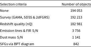
 \begin{equation} \tau^l_B = \tau_\beta - \tau_\alpha = \ln\left(\frac{\text{H}\alpha/\text{H}\beta}{2.86}\right)\end{equation}
(Calzetti, Kinney, & Storchi-Bergmann Reference Calzetti, Kinney and Storchi-Bergmann1994). The equation from Calzetti, Kinney, & Storchi-Bergmann (Reference Calzetti, Kinney and Storchi-Bergmann1994) used the value 2.88. Here we use 2.86 to remain consistent throughout the paper, although all results change only negligibly if the value 2.88 is used. Equation (2) can be rewritten as
 \begin{equation} \tau^l_B = 2.303\log\left(\frac{\text{H}\alpha}{\text{H}\beta}\right) - 1.0508.\end{equation}
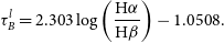
The geometry of dust with respect to stars is known to have an impact on the observed level of obscuration affecting a galaxy’s emission (e.g., Tuffs et al. Reference Tuffs, Popescu, Völk, Kylafis and Dopita2004; Natale et al. Reference Natale, Popescu, Tuffs, Debattista, Fischera and Grootes2015; Narayanan et al. Reference Narayanan, Conroy, Davé, Johnson and Popping2018; Lin et al. Reference Lin, Hirashita, Camps and Baes2021; Sachdeva & Nath Reference Sachdeva and Nath2022; Witt, Thronson, & Capuano Reference Witt and Thronson1992). In Figure 1, we present illustrations depicting two extreme versions of a dust geometry model. The first such model considered here, known as the foreground screen dust geometry model (Calzetti, Kinney, & Storchi-Bergmann Reference Calzetti, Kinney and Storchi-Bergmann1994), assumes that all the dust lies in a screen between the observer and the stars (Figure 1a-c). Figure 1a shows the case in which there is a low $M_d$
in a foreground screen geometry. In this scenario, there is little obscuration of the light. In Figure 1b, the increase in
$M_d$
in a foreground screen geometry. In this scenario, there is little obscuration of the light. In Figure 1b, the increase in $M_d$
results in greater obscuration due to the increased optical depth. In Figure 1c the
$M_d$
results in greater obscuration due to the increased optical depth. In Figure 1c the $M_d$
has increased to an extreme limit in which the optical depth is so great that any starlight is completely obscured.
$M_d$
has increased to an extreme limit in which the optical depth is so great that any starlight is completely obscured.
Diagram of different dust geometries. The observer lies to the right of each panel in this figure. Lightly coloured dust screens or clouds indicate low $M_d$
, and darker dust screens or clouds indicate higher
$M_d$
, and darker dust screens or clouds indicate higher $M_d$
. Blue stars (with many points) indicate little or no obscuration, green stars indicate mid to high obscuration, and red stars (with five points) indicate complete obscuration. Each panel in this figure represents a galaxy of the same size, such that an increase in dust mass results in an increase in optical depth.
$M_d$
. Blue stars (with many points) indicate little or no obscuration, green stars indicate mid to high obscuration, and red stars (with five points) indicate complete obscuration. Each panel in this figure represents a galaxy of the same size, such that an increase in dust mass results in an increase in optical depth.
In the distributed dust geometry model the dust and stars are mixed (Figure 1d-f). Figure 1d illustrates a scenario with low $M_d$
in a distributed geometry, resulting in little obscuration of the light. In Figure 1e the
$M_d$
in a distributed geometry, resulting in little obscuration of the light. In Figure 1e the $M_d$
, and therefore optical depth, are increased. The light from deeper within the cloud is more obscured due to travelling through more dust to reach the observer. Conversely, the light from the edges of the cloud closer to the observer are less obscured. In Figure 1f the
$M_d$
, and therefore optical depth, are increased. The light from deeper within the cloud is more obscured due to travelling through more dust to reach the observer. Conversely, the light from the edges of the cloud closer to the observer are less obscured. In Figure 1f the $M_d$
has been increased to an observational limit in which the light from deeper within the cloud is no longer detected. This light has been completely obscured. The light from the closer edges of the cloud, which travels through less dust, is less obscured, resulting in the detection of some obscured light.
$M_d$
has been increased to an observational limit in which the light from deeper within the cloud is no longer detected. This light has been completely obscured. The light from the closer edges of the cloud, which travels through less dust, is less obscured, resulting in the detection of some obscured light.
With the foreground screen geometry, all light of a given wavelength experiences consistent levels of obscuration, whether little or heavy obscuration, as it must travel through the same amount of dust. With a distributed dust geometry, light of a given wavelength from stars deeper within the cloud will experience more obscuration than light of the same wavelength from stars towards the edges of the cloud as the light from deeper within the cloud must travel through more dust. This means that the relative depth of stars within the dust cloud determines the level of obscuration, with deeper stars experiencing higher attenuation. Additionally, as the $M_d$
increases, a wider range of obscuration levels can be detected due to the varying positions of stars within the dust clouds.
$M_d$
increases, a wider range of obscuration levels can be detected due to the varying positions of stars within the dust clouds.
The level of obscuration within galaxies can be quantitatively assessed through the BD, while the optical depth is intrinsically connected to $M_d$
. Given this relationship, combining the BD and
$M_d$
. Given this relationship, combining the BD and $M_d$
offers a promising approach to investigate the intricate geometry of dust in galaxies. We use data from the Galaxy And Mass Assembly (GAMA) survey, described below, following which we introduce two novel parameters that link the BD and
$M_d$
offers a promising approach to investigate the intricate geometry of dust in galaxies. We use data from the Galaxy And Mass Assembly (GAMA) survey, described below, following which we introduce two novel parameters that link the BD and $M_d$
. These parameters aim to provide deeper insights into the role of dust geometry in influencing dust properties and SFRs.
$M_d$
. These parameters aim to provide deeper insights into the role of dust geometry in influencing dust properties and SFRs.
2.1 Data
The GAMA survey is a spectroscopic and photometric survey that covers approximately 250 deg $^2$
of the sky over 5 regions using the AAOmega spectrograph of the 3.9m Anglo-Australian Telescope (Driver et al. Reference Driver2011; Liske et al. Reference Liske2015; Driver et al. Reference Driver2016; Baldry et al. Reference Baldry2018; Driver et al. Reference Driver2022).
$^2$
of the sky over 5 regions using the AAOmega spectrograph of the 3.9m Anglo-Australian Telescope (Driver et al. Reference Driver2011; Liske et al. Reference Liske2015; Driver et al. Reference Driver2016; Baldry et al. Reference Baldry2018; Driver et al. Reference Driver2022).
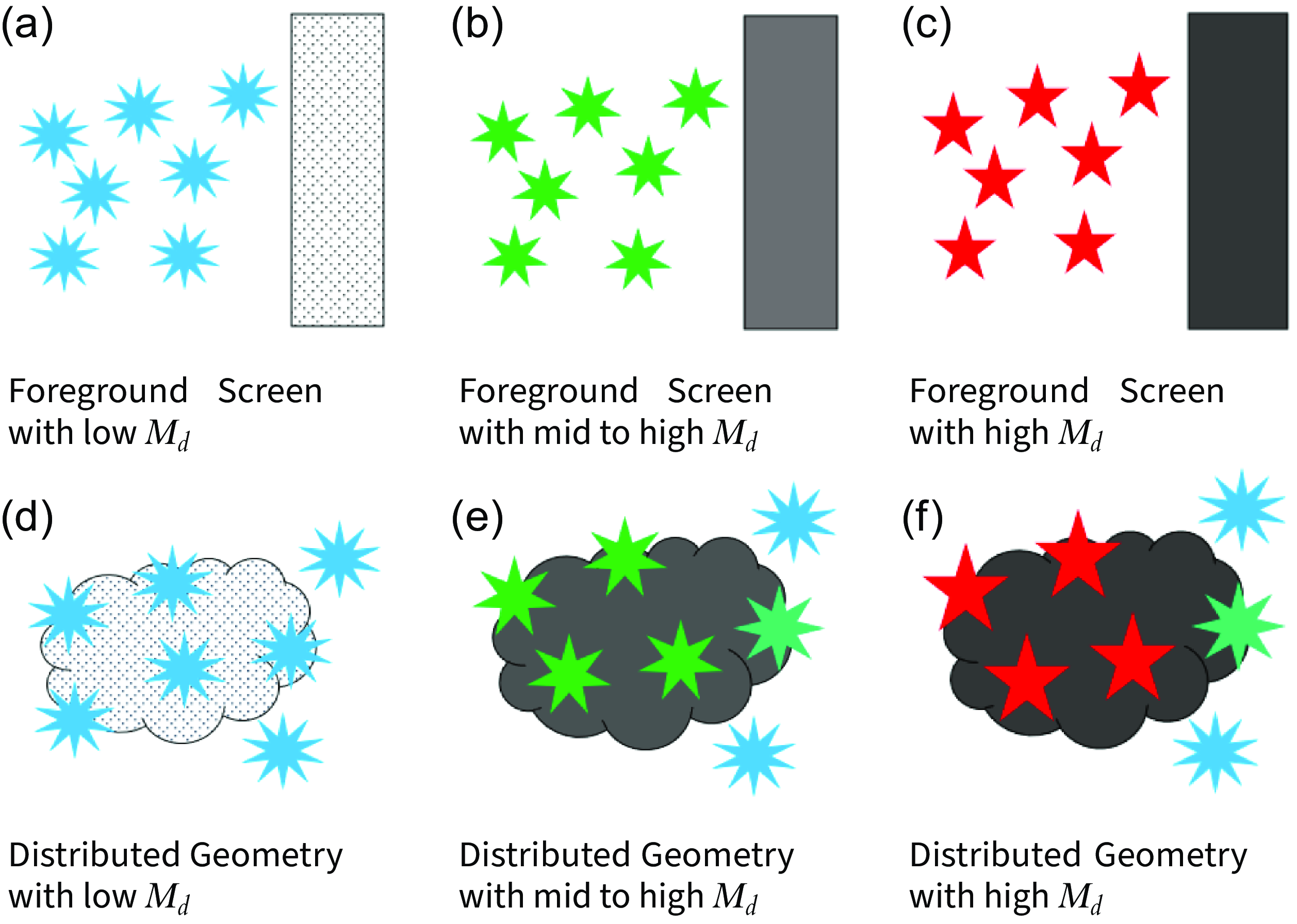
The GAMA data and derived parameters are organised into Data Management Units (DMUs, Liske et al. Reference Liske2015). We use data and derived parameters from various DMUs, detailed in Table 1. Specifically, emission line flux measurements and uncertainties for H $\alpha$
, H
$\alpha$
, H $\beta$
, N[ii], and O[iii], in addition to equivalent width measurements and uncertainties for the H
$\beta$
, N[ii], and O[iii], in addition to equivalent width measurements and uncertainties for the H $\alpha$
and H
$\alpha$
and H $\beta$
emission lines are obtained from the SpecLineSFR DMU (Gordon et al. Reference Gordon2017). The SpecLineSFR DMU also provides the original survey source and redshift estimates with redshift quality measures, nQ. The MAGPHYS DMU provides dust mass,
$\beta$
emission lines are obtained from the SpecLineSFR DMU (Gordon et al. Reference Gordon2017). The SpecLineSFR DMU also provides the original survey source and redshift estimates with redshift quality measures, nQ. The MAGPHYS DMU provides dust mass, $M_d$
, estimates and percentile ranges which were used to obtain the uncertainties on
$M_d$
, estimates and percentile ranges which were used to obtain the uncertainties on $M_d$
. While MAGPHYS is a robust tool for estimating dust masses, it is important to acknowledge that different SED models can yield systematically different
$M_d$
. While MAGPHYS is a robust tool for estimating dust masses, it is important to acknowledge that different SED models can yield systematically different $M_d$
estimates. The StellarMasses DMU (Taylor et al. Reference Taylor2011b) provides the stellar mass,
$M_d$
estimates. The StellarMasses DMU (Taylor et al. Reference Taylor2011b) provides the stellar mass, $M_*$
, estimates and uncertainties in addition to obscuration-corrected absolute magnitude measurements and uncertainties in the r band. The
$M_*$
, estimates and uncertainties in addition to obscuration-corrected absolute magnitude measurements and uncertainties in the r band. The $M_*$
estimates of Taylor et al. (Reference Taylor2011b) are based on the (Bruzual & Charlot Reference Bruzual and Charlot2003) population synthesis code, which is also used by MAGPHYS (da Cunha, Charlot, & Elbaz Reference da Cunha, Charlot and Elbaz2008; Taylor et al. Reference Taylor2011a). Uncorrected measurements and uncertainties for the r band and FUV band were also used. The FIR flux measurements and uncertainties were taken from the gkvFarIR DMU (Bellstedt et al. Reference Bellstedt2020b). The approximate elliptical semi-major axis and axial ratio values used to calculate the galaxy areas were obtained from the gkvInputCat DMU (Bellstedt et al. Reference Bellstedt2020a).
$M_*$
estimates of Taylor et al. (Reference Taylor2011b) are based on the (Bruzual & Charlot Reference Bruzual and Charlot2003) population synthesis code, which is also used by MAGPHYS (da Cunha, Charlot, & Elbaz Reference da Cunha, Charlot and Elbaz2008; Taylor et al. Reference Taylor2011a). Uncorrected measurements and uncertainties for the r band and FUV band were also used. The FIR flux measurements and uncertainties were taken from the gkvFarIR DMU (Bellstedt et al. Reference Bellstedt2020b). The approximate elliptical semi-major axis and axial ratio values used to calculate the galaxy areas were obtained from the gkvInputCat DMU (Bellstedt et al. Reference Bellstedt2020a).
Summary of the data and derived parameters used and their GAMA DMUs.
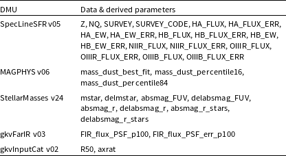
The sample used here was selected to ensure the data was of high quality. Only objects with redshifts originating from the GAMA, SDSS, and 2dFGRS surveys were used. The sample was limited to objects with redshift quality nQ $\geq$
3, which indicates a reliable estimate that is suitable for use in scientific analysis (Driver et al. Reference Driver2011). Only galaxies with lines in emission were retained, and the emission line flux measurements (H
$\geq$
3, which indicates a reliable estimate that is suitable for use in scientific analysis (Driver et al. Reference Driver2011). Only galaxies with lines in emission were retained, and the emission line flux measurements (H $\alpha$
, H
$\alpha$
, H $\beta$
, N[ii], O[iii]) were constrained to only those with a signal-to-noise ratio (S/N)
$\beta$
, N[ii], O[iii]) were constrained to only those with a signal-to-noise ratio (S/N) $\geq$
5. Similarly, the sample only contains dust mass estimates with S/N
$\geq$
5. Similarly, the sample only contains dust mass estimates with S/N $\geq$
3, and FIR flux measurements with S/N
$\geq$
3, and FIR flux measurements with S/N $\geq$
1. We use the standard optical diagnostic diagram of Baldwin, Phillips, & Terlevich (Reference Baldwin, Phillips and Terlevich1981) (BPT) to classify our galaxies as star forming or hosting active galactic nuclei (AGN). AGN were identified using the Kauffmann et al. (Reference Kauffmann2003) definition, and removed from our sample due to the significant effect AGN can have on the observed emission lines and the inferred properties of dust within galaxies. Table 2 shows how many objects remain after these various criteria are applied. Highly inclined galaxies are not removed from this sample. Less than 5% of the galaxies in this sample are moderately or highly inclined (with an axial ratio < 0.4), and removing these galaxies does not alter our results. Retaining these more highly inclined galaxies maintains the completeness of the sample and demonstrates that our analysis is not sensitive to inclination.
$\geq$
1. We use the standard optical diagnostic diagram of Baldwin, Phillips, & Terlevich (Reference Baldwin, Phillips and Terlevich1981) (BPT) to classify our galaxies as star forming or hosting active galactic nuclei (AGN). AGN were identified using the Kauffmann et al. (Reference Kauffmann2003) definition, and removed from our sample due to the significant effect AGN can have on the observed emission lines and the inferred properties of dust within galaxies. Table 2 shows how many objects remain after these various criteria are applied. Highly inclined galaxies are not removed from this sample. Less than 5% of the galaxies in this sample are moderately or highly inclined (with an axial ratio < 0.4), and removing these galaxies does not alter our results. Retaining these more highly inclined galaxies maintains the completeness of the sample and demonstrates that our analysis is not sensitive to inclination.
The number of objects remaining in the sample after each selection criteria was applied to the data.
2.2 BD, $\boldsymbol{M}_{\boldsymbol{d}}$
$\&$
dust geometry
$\boldsymbol{M}_{\boldsymbol{d}}$
$\&$
dust geometry


To quantify the BD we use the H $\alpha$
and H
$\alpha$
and H $\beta$
emission line flux measurements. These were first corrected for stellar absorption following Hopkins et al. (Reference Hopkins2003), as
$\beta$
emission line flux measurements. These were first corrected for stellar absorption following Hopkins et al. (Reference Hopkins2003), as
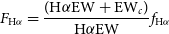 \begin{equation} F_{\text{H}\alpha} = \frac{(\text{H}\alpha \text{EW} + \text{EW}_c)}{\text{H}\alpha \text{EW}} f_{\text{H}\alpha}\end{equation}
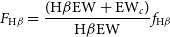 \begin{equation} F_{\text{H}\beta} = \frac{(\text{H}\beta \text{EW} + \text{EW}_c)}{\text{H}\beta \text{EW}} f_{\text{H}\beta}\end{equation}
where $f_{\text{H}\alpha}$
is the H
$f_{\text{H}\alpha}$
is the H $\alpha$
emission line flux,
$\alpha$
emission line flux, $f_{\text{H}\beta}$
is the H
$f_{\text{H}\beta}$
is the H $\beta$
emission line flux, H
$\beta$
emission line flux, H $\alpha$
EW is the equivalent width of the H
$\alpha$
EW is the equivalent width of the H $\alpha$
emission line, H
$\alpha$
emission line, H $\beta$
EW is the equivalent width of the H
$\beta$
EW is the equivalent width of the H $\beta$
emission line, and we adopt the same stellar absorption equivalent width correction for both H
$\beta$
emission line, and we adopt the same stellar absorption equivalent width correction for both H $\alpha$
and H
$\alpha$
and H $\beta$
of EW
$\beta$
of EW $_c$
= 2.5 following Gunawardhana et al. (Reference Gunawardhana2013). Finally, the BD values are calculated as
$_c$
= 2.5 following Gunawardhana et al. (Reference Gunawardhana2013). Finally, the BD values are calculated as
 \begin{equation} \text{BD} = \frac{F_{\text{H}\alpha}}{F_{\text{H}\beta}}.\end{equation}
The BD values calculated from each of GAMA, SDSS & 2dFGRS were compared to ensure that all three were providing consistent BD values within acceptable ranges. Although 2dFGRS spectra are not flux calibrated, the BD values are reliable, as they span the same range as those seen with the flux calibrated GAMA and SDSS spectra. If we omit them from our analysis our results remain unchanged apart from having slightly fewer galaxies represented.
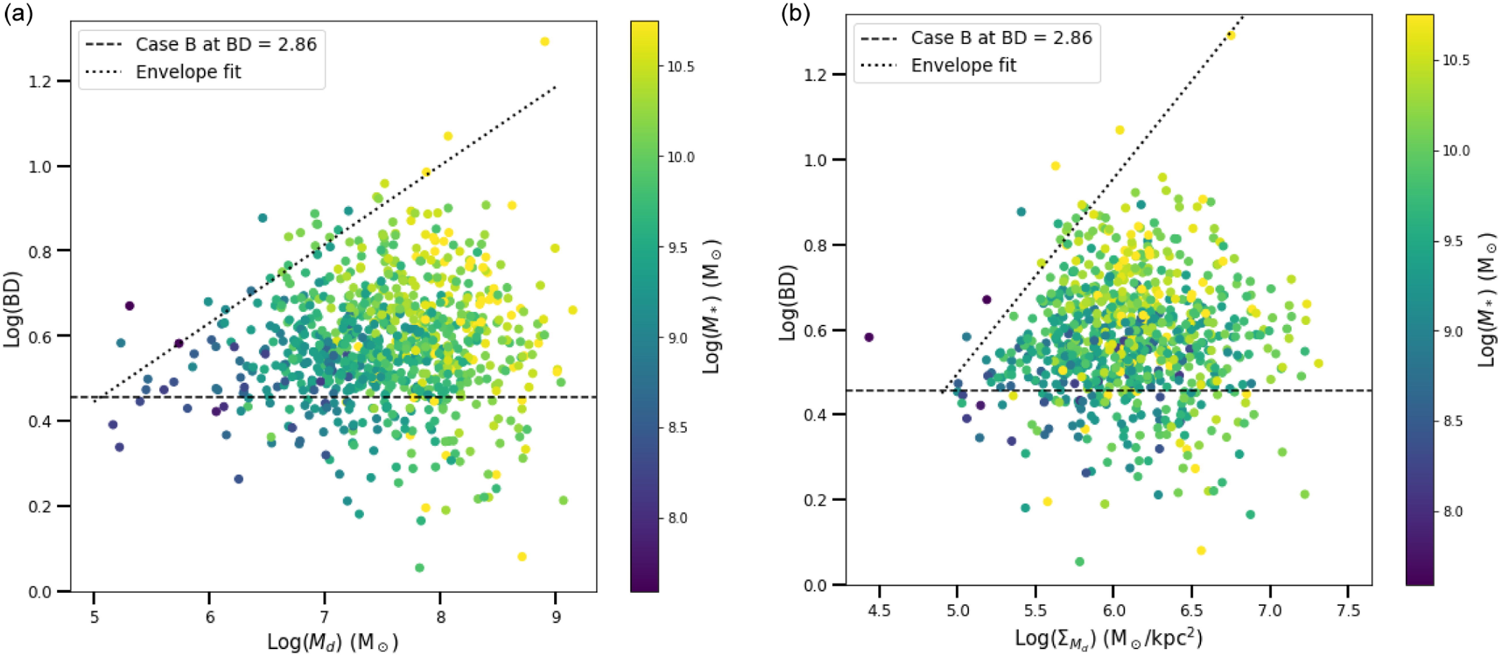
Figure 2 shows the relationship between the BD and both $M_d$
(Figure 2a) and dust surface density (
$M_d$
(Figure 2a) and dust surface density ( $\Sigma_{M_d}$
) (Figure 2b). There is an upper envelope for the observed BD values evident, which increases with increasing
$\Sigma_{M_d}$
) (Figure 2b). There is an upper envelope for the observed BD values evident, which increases with increasing $M_d$
and
$M_d$
and $\Sigma_{M_d}$
. The dotted lines shown tracing these envelopes are empirical characterisations. For this dataset, the two different envelope lines are given by:
$\Sigma_{M_d}$
. The dotted lines shown tracing these envelopes are empirical characterisations. For this dataset, the two different envelope lines are given by:
 \begin{equation} \log\!(\text{BD}_{\text{Env}}) = 0.185 \log(M_d) - 0.481,\end{equation}
and
 \begin{equation} \log\!(\text{BD}_{\text{Env}}) = 0.459 \log(\Sigma_{M_d}) - 1.801.\end{equation}
BD as a function of (a) $M_d$
, and (b) dust surface density, coloured by
$M_d$
, and (b) dust surface density, coloured by $M_*$
. The black dotted line represents the observed upper envelope of the data. The black dashed line represents the BD Case B value of 2.86. This Case B value of 2.86 is the BD value which corresponds to no obscuration (Osterbrock Reference Osterbrock1989). The correlation coefficient for panel (a) is 0.022 and the correlation coefficient for panel (b) is 0.013.
$M_*$
. The black dotted line represents the observed upper envelope of the data. The black dashed line represents the BD Case B value of 2.86. This Case B value of 2.86 is the BD value which corresponds to no obscuration (Osterbrock Reference Osterbrock1989). The correlation coefficient for panel (a) is 0.022 and the correlation coefficient for panel (b) is 0.013.
It is important to note that if different samples are being used, while qualitatively similar, such envelopes may differ quantitatively, especially if $M_d$
is estimated with different population synthesis tools.
$M_d$
is estimated with different population synthesis tools.
The envelope is not a consequence of the S/N limits placed on the dataset, as an envelope of the same shape is present even when no S/N limits are imposed. Investigating the H $\beta$
line flux as a function of
$\beta$
line flux as a function of $M_d$
does reveal that at the lowest values of
$M_d$
does reveal that at the lowest values of $M_d$
there is a tendency for the faintest H
$M_d$
there is a tendency for the faintest H $\beta$
fluxes to be absent. This, however, does not explain the existence of the envelope at the high
$\beta$
fluxes to be absent. This, however, does not explain the existence of the envelope at the high $M_d$
end, nor its relatively linear shape over the full range of
$M_d$
end, nor its relatively linear shape over the full range of $M_d$
. As a result, we are confident that the envelope seen here is not an observational bias, nor is it a result of our sample selection limits.
$M_d$
. As a result, we are confident that the envelope seen here is not an observational bias, nor is it a result of our sample selection limits.
In the case of Figure 2a this envelope traces the BD values resulting from a foreground screen geometry as the optical depth of the screen increases. We focus here on BD and $M_d$
for the purpose of this illustrative discussion of dust geometry. The low optical depth foreground screen geometry lies at the low BD, low
$M_d$
for the purpose of this illustrative discussion of dust geometry. The low optical depth foreground screen geometry lies at the low BD, low $M_d$
end of the envelope. The high optical depth foreground screen geometry lies at the high BD, high
$M_d$
end of the envelope. The high optical depth foreground screen geometry lies at the high BD, high $M_d$
end of the envelope. The models from Figure 1 are positioned in Figure 3, to capture their representative locations in the diagram, and to emphasise how each model would be reflected in the quantitative measurements.
$M_d$
end of the envelope. The models from Figure 1 are positioned in Figure 3, to capture their representative locations in the diagram, and to emphasise how each model would be reflected in the quantitative measurements.


In the case of low dust content, the foreground screen geometry and distributed geometry both fall in the low BD region, as neither provides enough attenuation to produce high BD measurements. This indicates that with less dust, the differences in geometries become more redundant in terms of their impact on the BD. However, even in low dust content scenarios, certain configurations of distributed geometry, such as those depicted in Figure 1f, can result in variations in the BD values.
There is a point at which the dust becomes so optically thick that the Balmer lines are too attenuated to escape. In the case of the foreground screen this results in no measurement of the Balmer lines at all, and corresponds to the high BD, high $M_d$
region that is lacking any data, as seen in the upper right of figures 2a and 3.
$M_d$
region that is lacking any data, as seen in the upper right of figures 2a and 3.
For the case of the distributed dust geometry, the emission lines from stars buried within the dust cloud escape less than emission at the outer boundary. This results in the emission lines originating in the edges of the cloud experiencing less attenuation and being observed, allowing for measurements that lie in the low BD, high $M_d$
region. Therefore, the data points along the Case B line, with a low BD, correspond to a maximal distributed dust geometry. A mixture of these two extreme dust geometries allows for the spread of values observed between the envelope line and the Case B line.
$M_d$
region. Therefore, the data points along the Case B line, with a low BD, correspond to a maximal distributed dust geometry. A mixture of these two extreme dust geometries allows for the spread of values observed between the envelope line and the Case B line.
It is well established that $M_d$
in galaxies is correlated with the
$M_d$
in galaxies is correlated with the $M_*$
. This is less the case for
$M_*$
. This is less the case for $\Sigma_{M_d}$
, and these relationships are shown together in Figure 4. Panel 4a shows the direct relationship between stellar mass and
$\Sigma_{M_d}$
, and these relationships are shown together in Figure 4. Panel 4a shows the direct relationship between stellar mass and $M_d$
, while panel 4c shows the ratio of
$M_d$
, while panel 4c shows the ratio of $M_d$
to stellar mass as a function of stellar mass. Panel 4b displays the relationship between
$M_d$
to stellar mass as a function of stellar mass. Panel 4b displays the relationship between $\Sigma_{M_d}$
and stellar mass. There is no panel that depicts the relationship between
$\Sigma_{M_d}$
and stellar mass. There is no panel that depicts the relationship between $\Sigma_{M_d}$
and
$\Sigma_{M_d}$
and $\Sigma_{M_*}$
as that would in effect be the same as panel 4a. However, panel 4d does show the ratio of
$\Sigma_{M_*}$
as that would in effect be the same as panel 4a. However, panel 4d does show the ratio of $\Sigma_{M_d}$
to
$\Sigma_{M_d}$
to $\Sigma_{M_*}$
as a function of
$\Sigma_{M_*}$
as a function of $\Sigma_{M_*}$
. These relationships are explored further by Cortese et al. (Reference Cortese2012), Clemens et al. (Reference Clemens2013), Calura et al. (Reference Calura2017), De Vis et al. (Reference De Vis2017), Orellana et al. (Reference Orellana2017), Casasola et al. (Reference Casasola2020); Casasola et al. (Reference Casasola2022). The trends in Figure 4 are colour coded by the SFR estimated from the H
$\Sigma_{M_*}$
. These relationships are explored further by Cortese et al. (Reference Cortese2012), Clemens et al. (Reference Clemens2013), Calura et al. (Reference Calura2017), De Vis et al. (Reference De Vis2017), Orellana et al. (Reference Orellana2017), Casasola et al. (Reference Casasola2020); Casasola et al. (Reference Casasola2022). The trends in Figure 4 are colour coded by the SFR estimated from the H $\alpha$
luminosity, which we calculate as follows. The obscuration corrected
$\alpha$
luminosity, which we calculate as follows. The obscuration corrected $L_{\text{H}\alpha}$
comes from
$L_{\text{H}\alpha}$
comes from
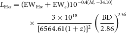 \begin{align} L_{\text{H}\alpha} &= (\text{EW}_{\text{H}\alpha} + \text{EW}_c) 10^{-0.4(M_r-34.10)}\nonumber \\ &\qquad \times\frac{3\times10^{18}}{[6564.61(1+z)]^2}\left(\frac{\text{BD}}{2.86}\right)^{\!\!2.36}\end{align}
where $M_r$
is the obscuration corrected r band absolute magnitude, and z is the redshift (Gunawardhana et al. Reference Gunawardhana2011, Reference Gunawardhana2013). If the observed BD is less than 2.86, then it is set to 2.86 here, equivalent to having no obscuration correction term. Equation (9) also includes terms that apply aperture and stellar absorption corrections, which are required for the H
$M_r$
is the obscuration corrected r band absolute magnitude, and z is the redshift (Gunawardhana et al. Reference Gunawardhana2011, Reference Gunawardhana2013). If the observed BD is less than 2.86, then it is set to 2.86 here, equivalent to having no obscuration correction term. Equation (9) also includes terms that apply aperture and stellar absorption corrections, which are required for the H $\alpha$
. The SFR
$\alpha$
. The SFR $_{\text{H}\alpha}$
is then calculated as
$_{\text{H}\alpha}$
is then calculated as
 \begin{equation} \text{SFR}_{\text{H}\alpha} = \frac{L_{\text{H}\alpha}}{1.27\times 10^{34}}\end{equation}
(Kennicutt Reference Kennicutt1998; Gunawardhana et al. Reference Gunawardhana2011).
(a) $M_d$
as a function of
$M_d$
as a function of $M_*$
, (b)
$M_*$
, (b) $\Sigma_{M_d}$
as a function of
$\Sigma_{M_d}$
as a function of $M_*$
, (c)
$M_*$
, (c) $M_d/M_*$
as a function of
$M_d/M_*$
as a function of $M_*$
, and (d)
$M_*$
, and (d) $\Sigma_{M_d}/\Sigma_{M_*}$
as a function of
$\Sigma_{M_d}/\Sigma_{M_*}$
as a function of $\Sigma_{M_*}$
, with all panels coloured by H
$\Sigma_{M_*}$
, with all panels coloured by H $\alpha$
SFR. The correlation coefficients are 0.66 for panel (a), 0.28 for panel (b), −0.032 for panel (c), and −0.47 for panel (d).
$\alpha$
SFR. The correlation coefficients are 0.66 for panel (a), 0.28 for panel (b), −0.032 for panel (c), and −0.47 for panel (d).

The $M_d$
and stellar mass are correlated, although with a scatter of about 1 dex around the broad trend. This is reflected in the relatively flat relationship seen in Figure 4c, albeit with the scatter emphasised in this representation. It is apparent that much of this scatter is related to the SFR. As the SFR increases with stellar mass, galaxies of a given dust mass with high SFRs have larger stellar masses than those with low SFRs. Figure 4d shows the ratio of surface densities for dust and stellar mass, which is actually identical to
$M_d$
and stellar mass are correlated, although with a scatter of about 1 dex around the broad trend. This is reflected in the relatively flat relationship seen in Figure 4c, albeit with the scatter emphasised in this representation. It is apparent that much of this scatter is related to the SFR. As the SFR increases with stellar mass, galaxies of a given dust mass with high SFRs have larger stellar masses than those with low SFRs. Figure 4d shows the ratio of surface densities for dust and stellar mass, which is actually identical to $M_d/M_*$
as the surface area term cancels. Looking at this parameter as a function of
$M_d/M_*$
as the surface area term cancels. Looking at this parameter as a function of $\Sigma_{M_*}$
, however, highlights that galaxies with the largest stellar mass surface density favour a lower proportion of dust mass, although the trend is mostly driven by the relatively small number of galaxies with
$\Sigma_{M_*}$
, however, highlights that galaxies with the largest stellar mass surface density favour a lower proportion of dust mass, although the trend is mostly driven by the relatively small number of galaxies with $\Sigma_{M_*} \gtrsim 10^9\,{\rm M}_{\odot}$
/kpc
$\Sigma_{M_*} \gtrsim 10^9\,{\rm M}_{\odot}$
/kpc $^2$
. This may suggest that the most compact galaxies may have proportionally less dust than more typical star forming galaxies. The interplay between stellar mass,
$^2$
. This may suggest that the most compact galaxies may have proportionally less dust than more typical star forming galaxies. The interplay between stellar mass, $M_d$
, and SFR implicitly includes the contribution of BD, as it is incorporated in the H
$M_d$
, and SFR implicitly includes the contribution of BD, as it is incorporated in the H $\alpha$
SFR estimate. In order to tease out these related parameters further, it is helpful to explore new ways of quantifying the links between BD,
$\alpha$
SFR estimate. In order to tease out these related parameters further, it is helpful to explore new ways of quantifying the links between BD, $M_d$
, and
$M_d$
, and $\Sigma_{M_d}$
. We start with an investigation of SFR estimators that are sensitive in different degrees to the presence of obscuring dust.
$\Sigma_{M_d}$
. We start with an investigation of SFR estimators that are sensitive in different degrees to the presence of obscuring dust.
3. The role of BD in understanding SFR tracers
Koyama et al. (Reference Koyama2015) studied the relationship between H $\alpha$
attenuation and the ratio of SFR
$\alpha$
attenuation and the ratio of SFR $_{\text{H}\alpha}$
to SFR
$_{\text{H}\alpha}$
to SFR $_{\text{FUV}}$
. This ratio can highlight the effect of optical depth due to the different effect at the different wavelengths. When the dust is more optically thick, proportionally less of the FUV emission will be detected, resulting in higher values of SFR
$_{\text{FUV}}$
. This ratio can highlight the effect of optical depth due to the different effect at the different wavelengths. When the dust is more optically thick, proportionally less of the FUV emission will be detected, resulting in higher values of SFR $_{\text{H}\alpha}$
/SFR
$_{\text{H}\alpha}$
/SFR $_{\text{FUV}}$
. Koyama et al. (Reference Koyama2015) found a positive correlation between the H
$_{\text{FUV}}$
. Koyama et al. (Reference Koyama2015) found a positive correlation between the H $\alpha$
attenuation and SFR
$\alpha$
attenuation and SFR $_{\text{H}\alpha}$
/SFR
$_{\text{H}\alpha}$
/SFR $_{\text{FUV}}$
, but noted that there is substantial scatter surrounding this relationship. Due to the scatter, they determined that dust attenuation levels could be roughly estimated using SFR
$_{\text{FUV}}$
, but noted that there is substantial scatter surrounding this relationship. Due to the scatter, they determined that dust attenuation levels could be roughly estimated using SFR $_{\text{H}\alpha}$
/SFR
$_{\text{H}\alpha}$
/SFR $_{\text{FUV}}$
, but that it could not be used as a more precise method of deriving the dust attenuation.
$_{\text{FUV}}$
, but that it could not be used as a more precise method of deriving the dust attenuation.
We reproduced their figure comparing H $\alpha$
attenuation and SFR
$\alpha$
attenuation and SFR $_{\text{H}\alpha}$
/SFR
$_{\text{H}\alpha}$
/SFR $_{\text{FUV}}$
, but instead used the BD rather than the H
$_{\text{FUV}}$
, but instead used the BD rather than the H $\alpha$
attenuation, as a starting point to explore the relationships surrounding dust geometry and optical depth (Figure 5a). This figure shows the relationship when no obscuration corrections are applied to the SFR estimates. For SFR
$\alpha$
attenuation, as a starting point to explore the relationships surrounding dust geometry and optical depth (Figure 5a). This figure shows the relationship when no obscuration corrections are applied to the SFR estimates. For SFR $_{\text{H}\alpha,Obs}$
, this simply corresponds to omitting the BD term from Equation (9). For SFR
$_{\text{H}\alpha,Obs}$
, this simply corresponds to omitting the BD term from Equation (9). For SFR $_{\text{FUV},Obs}$
we use
$_{\text{FUV},Obs}$
we use
 \begin{equation} L_{\text{FUV,Obs}} = 4\pi\text{D}_L^2 \times 10^{-0.4(m_{AB,\text{FUV}} + 56.1)}\end{equation}
where D $_L$
is the luminosity distance,
$_L$
is the luminosity distance, $m_{AB,\text{FUV}}$
is the FUV band apparent AB magnitude. This is converted to SFR through
$m_{AB,\text{FUV}}$
is the FUV band apparent AB magnitude. This is converted to SFR through
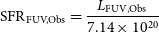 \begin{equation} \text{SFR}_{\text{FUV,Obs}} = \frac{L_{\text{FUV},\text{Obs}}}{7.14\times 10^{20}}\end{equation}
(Kennicutt Reference Kennicutt1998; Hopkins et al. Reference Hopkins2003).
(a) BD as a function of SFR $_{\text{H}\alpha, \text{Obs}}$
/SFR
$_{\text{H}\alpha, \text{Obs}}$
/SFR $_{\text{FUV, Obs}}$
, and (b) BD as a function of SFR
$_{\text{FUV, Obs}}$
, and (b) BD as a function of SFR $_{\text{H}\alpha}$
/SFR
$_{\text{H}\alpha}$
/SFR $_{\text{FUV}}$
, both coloured by
$_{\text{FUV}}$
, both coloured by $M_*$
. The correlation coefficient for panel (a) is 0.21 and the correlation coefficient for panel (b) is −0.399.
$M_*$
. The correlation coefficient for panel (a) is 0.21 and the correlation coefficient for panel (b) is −0.399.
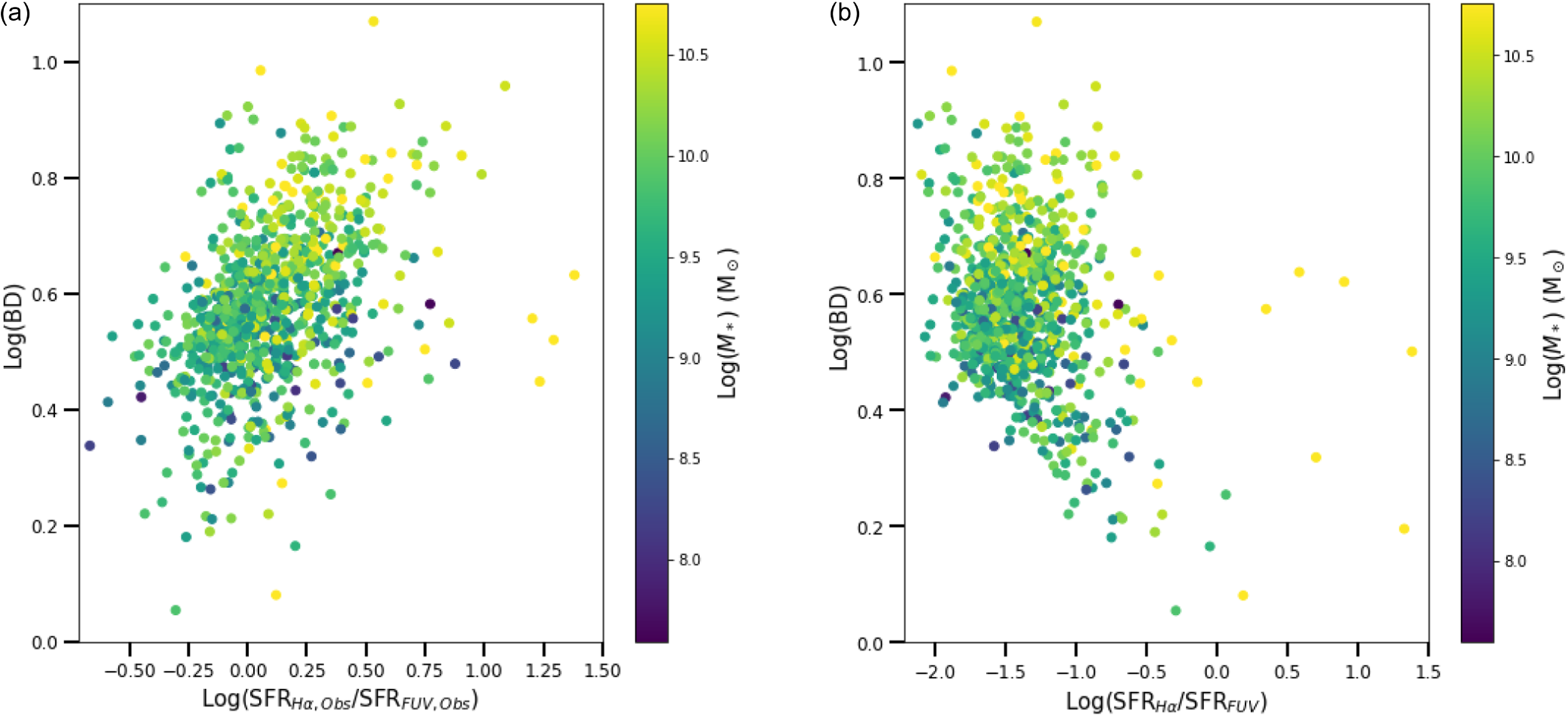
Figure 5a shows a positive correlation between the BD and SFR $_{\text{H}\alpha, \text{Obs}}$
/SFR
$_{\text{H}\alpha, \text{Obs}}$
/SFR $_{\text{FUV, Obs}}$
. This is expected as both are tracers of the obscuration present, consistent with the results of Koyama et al. (Reference Koyama2015). To implement an obscuration correction for SFR
$_{\text{FUV, Obs}}$
. This is expected as both are tracers of the obscuration present, consistent with the results of Koyama et al. (Reference Koyama2015). To implement an obscuration correction for SFR $_{\text{FUV}}$
, we follow Calzetti et al. (Reference Calzetti, Armus, Bohlin, Kinney, Koornneef and Storchi-Bergmann2000), using
$_{\text{FUV}}$
, we follow Calzetti et al. (Reference Calzetti, Armus, Bohlin, Kinney, Koornneef and Storchi-Bergmann2000), using
 \begin{equation} L_{\text{FUV}}(\lambda) = L_{\text{FUV,Obs}}(\lambda) 10^{0.4 E(B-V) k(\lambda)}\end{equation}
(Hopkins et al. Reference Hopkins, Connolly, Haarsma and Cram2001) where $k(\lambda)$
is the reddening curve (Calzetti et al. Reference Calzetti, Armus, Bohlin, Kinney, Koornneef and Storchi-Bergmann2000). For FUV the wavelength is
$k(\lambda)$
is the reddening curve (Calzetti et al. Reference Calzetti, Armus, Bohlin, Kinney, Koornneef and Storchi-Bergmann2000). For FUV the wavelength is $\lambda = 1\,500$
Å
$\lambda = 1\,500$
Å $ = 0.15\,\mu$
m and k(FUV) = 10.33.
$ = 0.15\,\mu$
m and k(FUV) = 10.33. $E(B-V)$
is given by
$E(B-V)$
is given by
 \begin{equation} E(B-V) = 0.44\frac{\log(\text{BD})}{0.4(k(\text{H}\beta)-k(\text{H}\alpha))}\end{equation}
(Calzetti Reference Calzetti2001a; Hopkins et al. Reference Hopkins, Connolly, Haarsma and Cram2001), with k(H $\alpha$
) = 2.38 and k(H
$\alpha$
) = 2.38 and k(H $\beta$
) = 3.65. The obscuration corrected SFR
$\beta$
) = 3.65. The obscuration corrected SFR $_{\text{FUV}}$
values are again calculated with the same SFR calibration factor
$_{\text{FUV}}$
values are again calculated with the same SFR calibration factor
 \begin{equation} \text{SFR}_{\text{FUV}} = \frac{L_{\text{FUV}}}{7.14\times 10^{20}}\end{equation}
(Kennicutt Reference Kennicutt1998; Hopkins et al. Reference Hopkins2003).
With obscuration corrections in place, the correlation between BD and SFR $_{\text{H}\alpha}$
/SFR
$_{\text{H}\alpha}$
/SFR $_{\text{FUV}}$
is no longer present (Figure 5b). This difference when the obscuration corrections are applied is a direct consequence of the degree of obscuration correction, and that the FUV measurements require a larger correction for a given value of BD compared to the H
$_{\text{FUV}}$
is no longer present (Figure 5b). This difference when the obscuration corrections are applied is a direct consequence of the degree of obscuration correction, and that the FUV measurements require a larger correction for a given value of BD compared to the H $\alpha$
measurements. This is reflected in the apparent lower diagonal envelope to the data distribution, where higher values of BD lead to proportionally higher SFR
$\alpha$
measurements. This is reflected in the apparent lower diagonal envelope to the data distribution, where higher values of BD lead to proportionally higher SFR $_\textrm{FUV}$
compared to SFR
$_\textrm{FUV}$
compared to SFR $_{\text{H}\alpha}$
. This causes the SFR ratio to decrease as BD increases, changing the positive correlation with the uncorrected ratio to a more or less vertical, uncorrelated, distribution. There is also a trend for galaxies of higher
$_{\text{H}\alpha}$
. This causes the SFR ratio to decrease as BD increases, changing the positive correlation with the uncorrected ratio to a more or less vertical, uncorrelated, distribution. There is also a trend for galaxies of higher $M_*$
to show higher BD, seen in the vertical colour gradient. This is expected from the fact that higher
$M_*$
to show higher BD, seen in the vertical colour gradient. This is expected from the fact that higher $M_*$
implies higher
$M_*$
implies higher $M_d$
, and high values of BD are only seen in high
$M_d$
, and high values of BD are only seen in high $M_d$
galaxies.
$M_d$
galaxies.
Instead of just investigating the H $\alpha$
and UV luminosities and their ratios, we can introduce other wavelength measurements as well. In particular the FIR emission is a well known tracer of the total dust-reradiated emission. We now use it as well in exploring this approach. Here we refer to the ratio of the FIR luminosity to the BD corrected H
$\alpha$
and UV luminosities and their ratios, we can introduce other wavelength measurements as well. In particular the FIR emission is a well known tracer of the total dust-reradiated emission. We now use it as well in exploring this approach. Here we refer to the ratio of the FIR luminosity to the BD corrected H $\alpha$
luminosity as the ‘H
$\alpha$
luminosity as the ‘H $\alpha$
deficit.” We choose this term since, if some degree of optically thick dust is present, the H
$\alpha$
deficit.” We choose this term since, if some degree of optically thick dust is present, the H $\alpha$
luminosity will be reduced in comparison to the FIR luminosity. In the absence of optically thick dust affecting the H
$\alpha$
luminosity will be reduced in comparison to the FIR luminosity. In the absence of optically thick dust affecting the H $\alpha$
, the two should be proportional, both tracing the underlying SFR.
$\alpha$
, the two should be proportional, both tracing the underlying SFR.
The FIR luminosity is calculated simply with
 \begin{equation} L_{\text{FIR}} = 4\pi\text{D}_L^2 \times f_{\text{FIR}}\end{equation}
where $f_{\text{FIR}}$
is the Herschel-ATLAS
$f_{\text{FIR}}$
is the Herschel-ATLAS $100\,\mu$
m flux, and D
$100\,\mu$
m flux, and D $_L$
is the luminosity distance. These results are qualitatively unchanged if we use the
$_L$
is the luminosity distance. These results are qualitatively unchanged if we use the $160\,\mu$
m flux instead, or a linear combination of both. We choose to present the results here in terms of a single FIR band for simplicity. At this stage, we are ready to return to quantifying links between the BD,
$160\,\mu$
m flux instead, or a linear combination of both. We choose to present the results here in terms of a single FIR band for simplicity. At this stage, we are ready to return to quantifying links between the BD, $M_d$
, and
$M_d$
, and $\Sigma_{M_d}$
.
$\Sigma_{M_d}$
.
4. A new approach
To link the BD with the $M_d$
and
$M_d$
and $\Sigma_{M_d}$
, we introduce two new parameters. The first of these is a new parameter aimed at quantifying the mixing of the foreground screen and distributed dust geometries. This parameter,
$\Sigma_{M_d}$
, we introduce two new parameters. The first of these is a new parameter aimed at quantifying the mixing of the foreground screen and distributed dust geometries. This parameter, $F_\textrm{dust}$
, is calculated as
$F_\textrm{dust}$
, is calculated as
 \begin{equation} F_\textrm{dust} = \frac{\log\text{BD}-\log(2.86)}{\log\text{BD}_{\text{Env}}-\log(2.86)}\end{equation}
where BD $_{\text{Env}}$
is the BD value at the envelope line from Figure 2a (Equation 7).
$_{\text{Env}}$
is the BD value at the envelope line from Figure 2a (Equation 7). $F_\textrm{dust}$
quantifies where a BD value lies vertically in relation to the Case B and envelope lines. In doing so, it quantifies the proportion that each geometry contributes in that galaxy, with higher values of
$F_\textrm{dust}$
quantifies where a BD value lies vertically in relation to the Case B and envelope lines. In doing so, it quantifies the proportion that each geometry contributes in that galaxy, with higher values of $F_\textrm{dust}$
indicating a more foreground screen geometry and lower values of
$F_\textrm{dust}$
indicating a more foreground screen geometry and lower values of $F_\textrm{dust}$
indicating a more distributed geometry. A value of
$F_\textrm{dust}$
indicating a more distributed geometry. A value of $F_\textrm{dust}=1$
may be referred to as a ‘maximal foreground screen’ geometry, and
$F_\textrm{dust}=1$
may be referred to as a ‘maximal foreground screen’ geometry, and $F_\textrm{dust}=0$
as a ‘maximal distributed dust’ geometry. In our sample, for the small number of galaxies with BD lying above the envelope line or below the Case B line, we set
$F_\textrm{dust}=0$
as a ‘maximal distributed dust’ geometry. In our sample, for the small number of galaxies with BD lying above the envelope line or below the Case B line, we set $F_\textrm{dust}$
to be 1 or 0 respectively.
$F_\textrm{dust}$
to be 1 or 0 respectively.
It is important to acknowledge that the terms ‘foreground screen’ and ‘distributed dust’ are used as convenient descriptors of dust distribution regimes and should not be interpreted literally. The primary distinction is that the ‘distributed dust’ regime can result in significant portions of the SFR and associated Balmer lines being entirely obscured by dust, while other regions experience only slight extinction. As a result, the BD can be small despite substantial loss of H $\alpha$
emission. In contrast, the ‘foreground screen’ regime implies a moderate and more uniform obscuration of all emission regions, leading to a larger BD while still allowing a considerable amount of H
$\alpha$
emission. In contrast, the ‘foreground screen’ regime implies a moderate and more uniform obscuration of all emission regions, leading to a larger BD while still allowing a considerable amount of H $\alpha$
emission to be observed.
$\alpha$
emission to be observed.
Since Figure 2b shows a similar structure with an envelope line, a version of $F_\textrm{dust}$
may also be calculated from this
$F_\textrm{dust}$
may also be calculated from this $\Sigma_{M_d}$
version of the figure. The version of
$\Sigma_{M_d}$
version of the figure. The version of $F_\textrm{dust}$
calculated from the
$F_\textrm{dust}$
calculated from the $\Sigma_{M_d}$
figure (Figure 2b) will be referred to as
$\Sigma_{M_d}$
figure (Figure 2b) will be referred to as $\Sigma_{F_\textrm{dust}}$
and uses BD
$\Sigma_{F_\textrm{dust}}$
and uses BD $_{\text{Env}}$
from Equation (8).
$_{\text{Env}}$
from Equation (8).
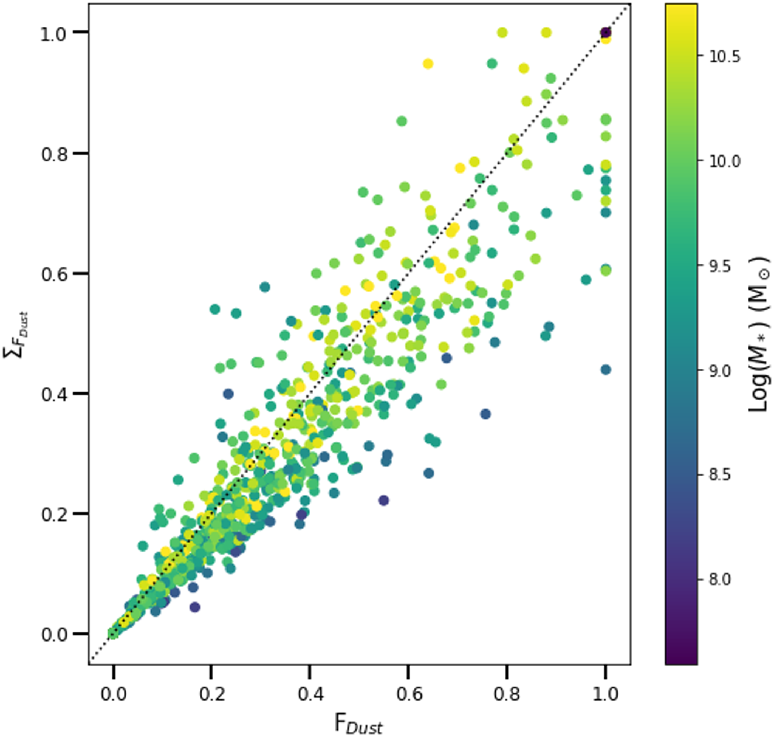
Figure 6 compares the $F_\textrm{dust}$
and
$F_\textrm{dust}$
and $\Sigma_{F_\textrm{dust}}$
values. The data are centred quite evenly around the 1:1 line, although there is a slight tendency towards somewhat higher
$\Sigma_{F_\textrm{dust}}$
values. The data are centred quite evenly around the 1:1 line, although there is a slight tendency towards somewhat higher $F_\textrm{dust}$
values compared to
$F_\textrm{dust}$
values compared to $\Sigma_{F_\textrm{ dust}}$
. The mostly even distribution about the 1:1 line indicates that
$\Sigma_{F_\textrm{ dust}}$
. The mostly even distribution about the 1:1 line indicates that $F_\textrm{dust}$
and
$F_\textrm{dust}$
and $\Sigma_{F_\textrm{ dust}}$
are sufficiently similar that either may be used in exploring dust geometry. However, it is worth noting that the interpretation of the envelope line in these diagrams cannot imply the same dust geometry in both cases. We argue that
$\Sigma_{F_\textrm{ dust}}$
are sufficiently similar that either may be used in exploring dust geometry. However, it is worth noting that the interpretation of the envelope line in these diagrams cannot imply the same dust geometry in both cases. We argue that $F_\textrm{dust}$
is the choice that better matches a model where the envelope line represents a foreground screen dust geometry.
$F_\textrm{dust}$
is the choice that better matches a model where the envelope line represents a foreground screen dust geometry. $\Sigma_{F_\textrm{dust}}$
as a function of
$\Sigma_{F_\textrm{dust}}$
as a function of $F_\textrm{dust}$
, coloured by
$F_\textrm{dust}$
, coloured by $M_*$
. The dotted line is a 1:1 line. The correlation coefficient is 0.94.
$M_*$
. The dotted line is a 1:1 line. The correlation coefficient is 0.94.
Independent of any envelope line, the BD and $M_d$
may still be combined in such a way that more information about the geometry and optical depth of the dust may be inferred than if they are used independently. We introduce a second new parameter,
$M_d$
may still be combined in such a way that more information about the geometry and optical depth of the dust may be inferred than if they are used independently. We introduce a second new parameter, $H_\textrm{dust}$
, that links the BD and
$H_\textrm{dust}$
, that links the BD and $M_d$
in a different way, in order to quantify the dust geometry.
$M_d$
in a different way, in order to quantify the dust geometry. $H_\textrm{dust}$
is defined in terms of the BD as
$H_\textrm{dust}$
is defined in terms of the BD as
 \begin{equation} H_\textrm{dust} = 10^{1.0508}\frac{M_d}{\text{BD}^{2.303}}.\end{equation}
Equation (18) was derived using
 \begin{equation} H_\textrm{dust} = \frac{M_d}{10^{\tau^l_B}}\end{equation}
which is equivalent in the case of a foreground screen geometry. Therefore, $H_\textrm{dust}$
can be interpreted as a normalised dust mass, providing a way to quantify dust geometry beyond using BD and
$H_\textrm{dust}$
can be interpreted as a normalised dust mass, providing a way to quantify dust geometry beyond using BD and $M_d$
independently. As with
$M_d$
independently. As with $F_\textrm{dust}$
, an alternate version of
$F_\textrm{dust}$
, an alternate version of $H_\textrm{dust}$
can be calculated in which
$H_\textrm{dust}$
can be calculated in which $\Sigma_{M_d}$
is used in place of
$\Sigma_{M_d}$
is used in place of $M_d$
. This dust surface density version will be referred to as
$M_d$
. This dust surface density version will be referred to as $\Sigma_{H_\textrm{dust}}$
.
$\Sigma_{H_\textrm{dust}}$
.
Figure 7 compares $H_\textrm{dust}$
and
$H_\textrm{dust}$
and $\Sigma_{H_\textrm{dust}}$
. Although the
$\Sigma_{H_\textrm{dust}}$
. Although the $H_\textrm{dust}$
values are consistently higher than the
$H_\textrm{dust}$
values are consistently higher than the $\Sigma_{H_\textrm{dust}}$
values, the two parameters are still correlated. For the purposes of this investigation
$\Sigma_{H_\textrm{dust}}$
values, the two parameters are still correlated. For the purposes of this investigation $H_\textrm{dust}$
is the more intuitive quantity.
$H_\textrm{dust}$
is the more intuitive quantity. $H_\textrm{dust}$
is a global parameter as it uses the total dust content of the galaxy, whereas
$H_\textrm{dust}$
is a global parameter as it uses the total dust content of the galaxy, whereas $\Sigma_{H_\textrm{dust}}$
, using a surface density, is related to the spatial distribution of the dust. In this analysis we are interested in exploring parameters like star formation and dust geometry as global galaxy properties. Were another study to be conducted focusing on surface densities and the spatial distribution of galaxy properties, then perhaps
$\Sigma_{H_\textrm{dust}}$
, using a surface density, is related to the spatial distribution of the dust. In this analysis we are interested in exploring parameters like star formation and dust geometry as global galaxy properties. Were another study to be conducted focusing on surface densities and the spatial distribution of galaxy properties, then perhaps $\Sigma_{H_\textrm{dust}}$
would be the more useful parameter.
$\Sigma_{H_\textrm{dust}}$
would be the more useful parameter. $\Sigma_{H_\textrm{dust}}$
as a function of
$\Sigma_{H_\textrm{dust}}$
as a function of $H_\textrm{dust}$
, coloured by
$H_\textrm{dust}$
, coloured by $M_*$
. The dotted line is a 1:1 line. The correlation coefficient is 0.77.
$M_*$
. The dotted line is a 1:1 line. The correlation coefficient is 0.77.

Seeing as the dust mass and dust surface density definitions of F and H are correlated with one another, either may be used and yield similar results. To avoid repetition and eliminate redundancy, this analysis continues with only one set. As discussed above, $F_\textrm{dust}$
and
$F_\textrm{dust}$
and $H_\textrm{dust}$
provide the more intuitive choice for this investigation. Thus, the remainder of this analysis focuses on
$H_\textrm{dust}$
provide the more intuitive choice for this investigation. Thus, the remainder of this analysis focuses on $F_\textrm{dust}$
and
$F_\textrm{dust}$
and $H_\textrm{dust}$
.
$H_\textrm{dust}$
.
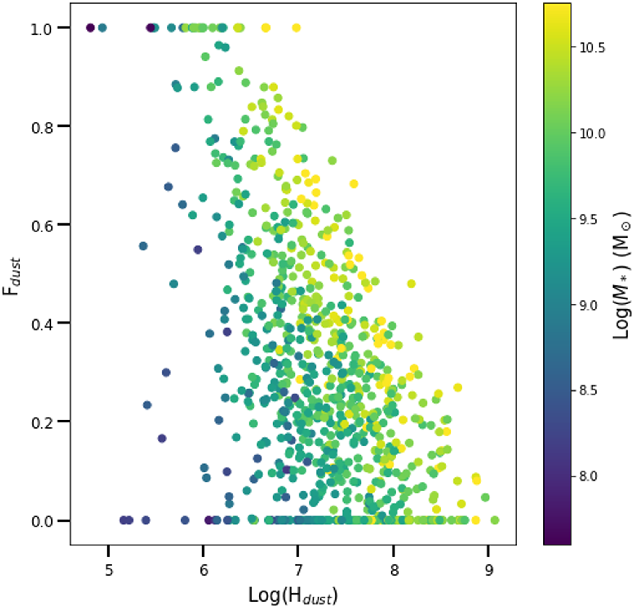
Figure 8 presents the relationship between $F_\textrm{dust}$
and
$F_\textrm{dust}$
and $H_\textrm{dust}$
, showing a negative correlation, as expected from the way the two parameters are defined. There is a strong
$H_\textrm{dust}$
, showing a negative correlation, as expected from the way the two parameters are defined. There is a strong $M_*$
dependence visible, in the sense that the inverse correlation between
$M_*$
dependence visible, in the sense that the inverse correlation between $F_\textrm{dust}$
and
$F_\textrm{dust}$
and $H_\textrm{dust}$
moves to higher values of
$H_\textrm{dust}$
moves to higher values of $H_\textrm{dust}$
as
$H_\textrm{dust}$
as $M_*$
increases. Galaxies with higher
$M_*$
increases. Galaxies with higher $F_\textrm{dust}$
tend to have lower values of
$F_\textrm{dust}$
tend to have lower values of $H_\textrm{dust}$
. High
$H_\textrm{dust}$
. High $F_\textrm{dust}$
and low
$F_\textrm{dust}$
and low $H_\textrm{dust}$
correspond to a more foreground screen dust geometry with more optically thin dust. For galaxies with lower values of
$H_\textrm{dust}$
correspond to a more foreground screen dust geometry with more optically thin dust. For galaxies with lower values of $F_\textrm{dust}$
, the spread of
$F_\textrm{dust}$
, the spread of $H_\textrm{dust}$
values increases. This indicates that as the geometry moves towards a greater proportion of distributed dust, there is greater variation in the optical depth observed. A numerical quantification of the anticorrelation between
$H_\textrm{dust}$
values increases. This indicates that as the geometry moves towards a greater proportion of distributed dust, there is greater variation in the optical depth observed. A numerical quantification of the anticorrelation between $F_\textrm{dust}$
and
$F_\textrm{dust}$
and $H_\textrm{dust}$
is not especially illuminating, as this will be dependent on the specific choice of envelope line, which in turn will be dependent on the specific sample being used, and the determination of dust masses.
$H_\textrm{dust}$
is not especially illuminating, as this will be dependent on the specific choice of envelope line, which in turn will be dependent on the specific sample being used, and the determination of dust masses. $F_\textrm{dust}$
as a function of
$F_\textrm{dust}$
as a function of $H_\textrm{dust}$
, coloured by
$H_\textrm{dust}$
, coloured by $M_*$
. The correlation coefficient is −0.56.
$M_*$
. The correlation coefficient is −0.56.
We can use another approach to consider the qualitative geometry of the dust as well. If we assume the simplest scenario, that every galaxy has dust arranged in a foreground screen, that has an implication for how we can interpret $\Sigma_{M_d}$
. This can be thought of as representing the thickness of the screen, if we consider the dust mass,
$\Sigma_{M_d}$
. This can be thought of as representing the thickness of the screen, if we consider the dust mass, $M_d$
, as representative of the volume over which it is spread. In this scenario, we would expect that the BD would be correlated with
$M_d$
, as representative of the volume over which it is spread. In this scenario, we would expect that the BD would be correlated with $\Sigma_{M_d}$
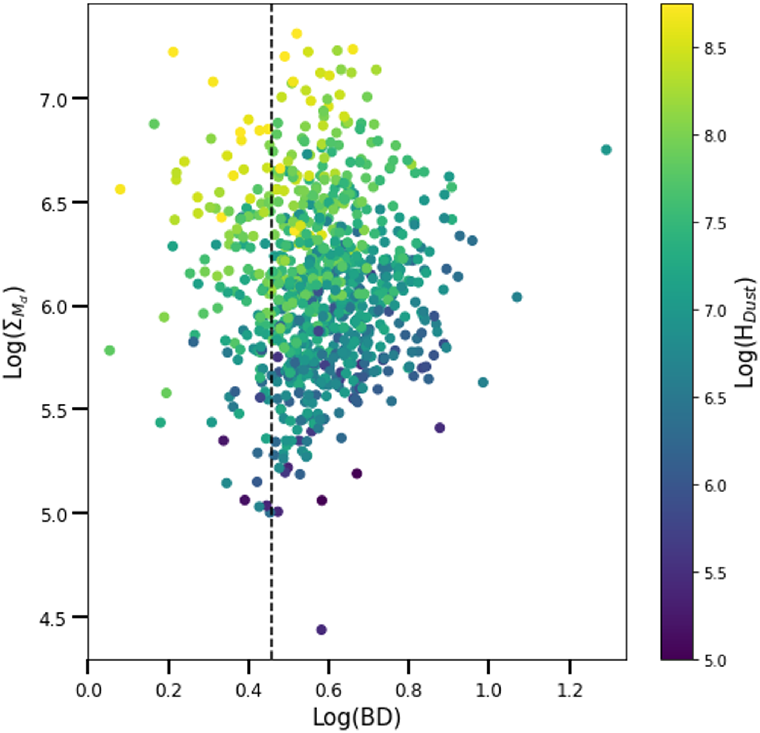
, since a thicker screen would produce a larger BD. We explore this explicitly in Figure 9, which shows
$\Sigma_{M_d}$
, since a thicker screen would produce a larger BD. We explore this explicitly in Figure 9, which shows $\Sigma_{M_d}$
as a function of BD, coloured by
$\Sigma_{M_d}$
as a function of BD, coloured by $H_\textrm{dust}$
. We can see here that there is no correlation between
$H_\textrm{dust}$
. We can see here that there is no correlation between $\Sigma_{M_d}$
and BD, with the possible exception of galaxies with the lowest
$\Sigma_{M_d}$
and BD, with the possible exception of galaxies with the lowest $H_\textrm{dust}$
. Galaxies with the highest
$H_\textrm{dust}$
. Galaxies with the highest $H_\textrm{dust}$
show the largest
$H_\textrm{dust}$
show the largest $\Sigma_{M_d}$
values, but are restricted to a narrow range of the lowest BD. If the foreground screen interpretation is correct we would expect the thickest screen (largest
$\Sigma_{M_d}$
values, but are restricted to a narrow range of the lowest BD. If the foreground screen interpretation is correct we would expect the thickest screen (largest $\Sigma_{M_d}$
) to have the highest BD, but this is not the case. Accordingly, this implies that these galaxies do not favour a foreground screen geometry, and our interpretation of them as having dust that is mixed and distributed throughout the galaxy is more likely. This permits low BD values to arise from the edges of the dust distribution, where low levels of obscuration can occur. The model proposed above (Figure 3) is supported by this result. Subsequently, we continue with our interpretation that galaxies with low BD, high
$\Sigma_{M_d}$
) to have the highest BD, but this is not the case. Accordingly, this implies that these galaxies do not favour a foreground screen geometry, and our interpretation of them as having dust that is mixed and distributed throughout the galaxy is more likely. This permits low BD values to arise from the edges of the dust distribution, where low levels of obscuration can occur. The model proposed above (Figure 3) is supported by this result. Subsequently, we continue with our interpretation that galaxies with low BD, high $M_d$
, and thus high
$M_d$
, and thus high $H_\textrm{dust}$
, have a distributed dust geometry. This in turn is associated with dust that is more optically thick to H
$H_\textrm{dust}$
, have a distributed dust geometry. This in turn is associated with dust that is more optically thick to H $\alpha$
emission.
$\alpha$
emission. $\Sigma_{M_d}$
as a function of BD, coloured by
$\Sigma_{M_d}$
as a function of BD, coloured by $H_\textrm{dust}$
. The dashed line represents the Case B value at BD = 2.86. The correlation coefficient is 0.013.
$H_\textrm{dust}$
. The dashed line represents the Case B value at BD = 2.86. The correlation coefficient is 0.013.
We now have two parameters which each provide a new way to quantify the optical depth and geometry of a galaxy’s dust, with $F_\textrm{ dust}$
being more directly related to the geometry and
$F_\textrm{ dust}$
being more directly related to the geometry and $H_\textrm{dust}$
being more directly related to the optical depth. The following analysis explores how these parameters are related to other observational quantities which are themselves expected to strongly trace the degree of optical depth of the dust.
$H_\textrm{dust}$
being more directly related to the optical depth. The following analysis explores how these parameters are related to other observational quantities which are themselves expected to strongly trace the degree of optical depth of the dust.
5. Results
There is no correlation seen between $H_\textrm{dust}$
or
$H_\textrm{dust}$
or $F_\textrm{dust}$
and SFR
$F_\textrm{dust}$
and SFR $_{\text{H}\alpha}$
/SFR
$_{\text{H}\alpha}$
/SFR $_{\text{FUV}}$
(Figure 10). The notable difference between Figs. 10a and 10b is that
$_{\text{FUV}}$
(Figure 10). The notable difference between Figs. 10a and 10b is that $H_\textrm{dust}$
shows a dependence on
$H_\textrm{dust}$
shows a dependence on $M_*$
, but
$M_*$
, but $F_\textrm{dust}$
does not. This is a direct result of the way the two parameters are defined.
$F_\textrm{dust}$
does not. This is a direct result of the way the two parameters are defined. $H_\textrm{dust}$
is defined such that it is strongly correlated to the
$H_\textrm{dust}$
is defined such that it is strongly correlated to the $M_d$
, and therefore also (indirectly) to the stellar mass (Figure 4a).
$M_d$
, and therefore also (indirectly) to the stellar mass (Figure 4a). $F_\textrm{dust}$
is defined in such a way that although it is mathematically dependent on the
$F_\textrm{dust}$
is defined in such a way that although it is mathematically dependent on the $M_d$
(through the BD envelope line), it is not strongly correlated with the
$M_d$
(through the BD envelope line), it is not strongly correlated with the $M_d$
(or
$M_d$
(or $M_*$
).
$M_*$
).
The relationships between SFR $_{\text{H}\alpha}$
/SFR
$_{\text{H}\alpha}$
/SFR $_{\text{FUV}}$
and (a)
$_{\text{FUV}}$
and (a) $H_\textrm{dust}$
, and (b)
$H_\textrm{dust}$
, and (b) $F_\textrm{dust}$
, each coloured by
$F_\textrm{dust}$
, each coloured by $M_*$
. The correlation coefficient for panel (a) is 0.093 and the correlation coefficient for panel (b) is −0.14.
$M_*$
. The correlation coefficient for panel (a) is 0.093 and the correlation coefficient for panel (b) is −0.14.
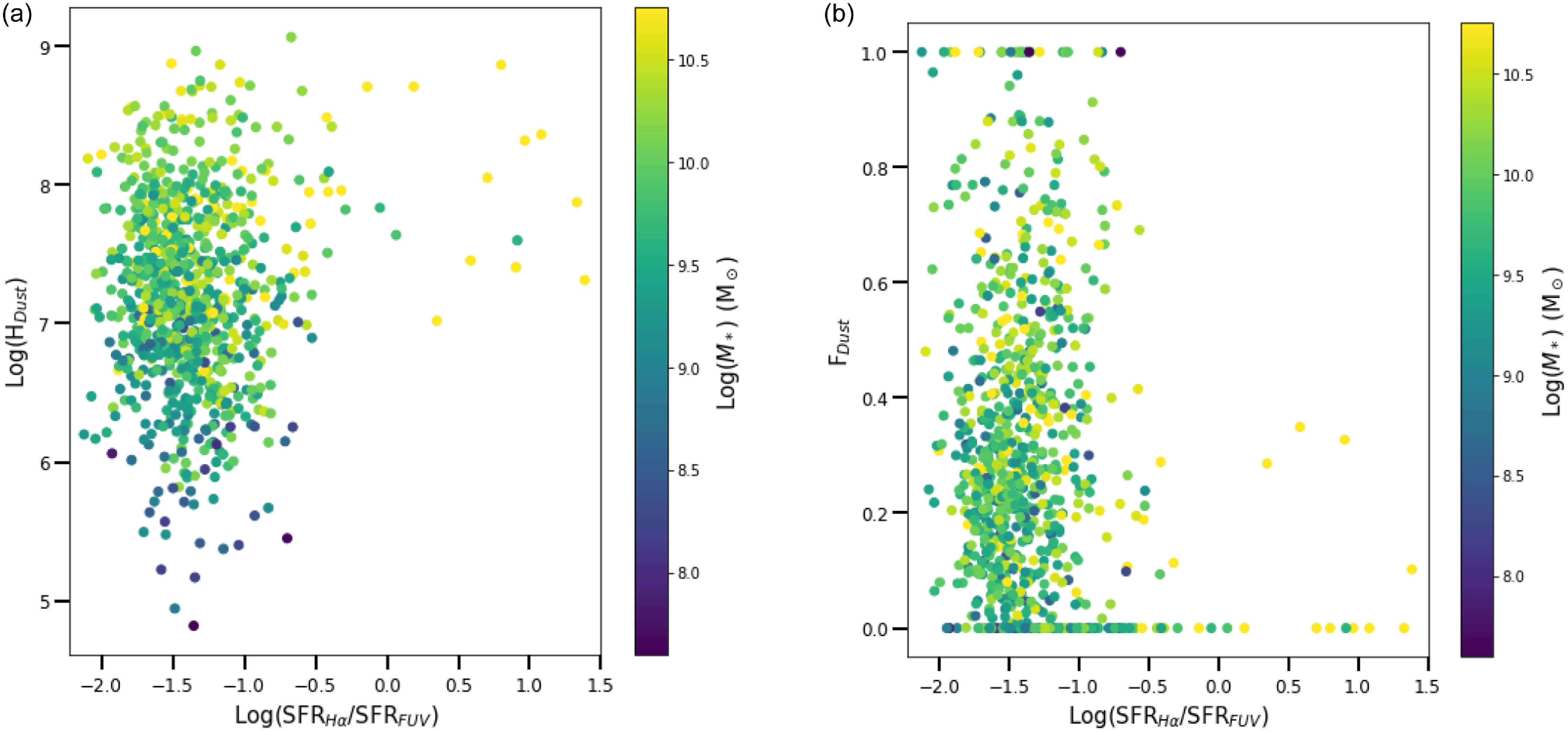
The lack of trend in Figure 10a and 10b indicates that the H $\alpha$
and FUV are experiencing a similar degree of optically thick dust. This implies that the stars and the gas are closely co-located, with the optically thick effects impacting both to the same degree. If this were not the case, and the emission from the stars and gas were experiencing different levels of obscuration, then Figure 10a would show a positive correlation between
$\alpha$
and FUV are experiencing a similar degree of optically thick dust. This implies that the stars and the gas are closely co-located, with the optically thick effects impacting both to the same degree. If this were not the case, and the emission from the stars and gas were experiencing different levels of obscuration, then Figure 10a would show a positive correlation between $H_\textrm{ dust}$
and SFR
$H_\textrm{ dust}$
and SFR $_{\text{H}\alpha}$
/SFR
$_{\text{H}\alpha}$
/SFR $_{\text{FUV}}$
, while Figure 10b would show a negative trend.
$_{\text{FUV}}$
, while Figure 10b would show a negative trend.
To further explore the relationships between $H_\textrm{dust}$
,
$H_\textrm{dust}$
, $F_\textrm{dust}$
, and the H
$F_\textrm{dust}$
, and the H $\alpha$
deficit, we define four independent mass-limited redshift bins. The full sample spans a redshift range
$\alpha$
deficit, we define four independent mass-limited redshift bins. The full sample spans a redshift range $0\lt z\lt 0.35$
. The redshift bins were defined as shown in Figure 11 and Table 3.
$0\lt z\lt 0.35$
. The redshift bins were defined as shown in Figure 11 and Table 3.
The four volume-limited samples used to explore any redshift and mass dependencies.

The number of objects in each of the mass-limited redshift bins.
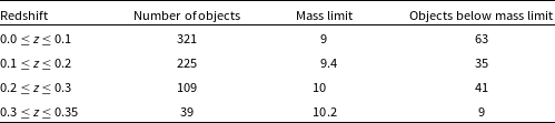
Figure 12a and 12b show the relationships between $H_\textrm{dust}$
and
$H_\textrm{dust}$
and $F_\textrm{dust}$
with the H
$F_\textrm{dust}$
with the H $\alpha$
deficit.
$\alpha$
deficit. $H_\textrm{dust}$
has a positive correlation with the H
$H_\textrm{dust}$
has a positive correlation with the H $\alpha$
deficit, whereas
$\alpha$
deficit, whereas $F_\textrm{dust}$
has a negative correlation. These opposing trends are expected due to the negative correlation between
$F_\textrm{dust}$
has a negative correlation. These opposing trends are expected due to the negative correlation between $H_\textrm{dust}$
and
$H_\textrm{dust}$
and $F_\textrm{dust}$
(Figure 8). Higher H
$F_\textrm{dust}$
(Figure 8). Higher H $\alpha$
deficit values reflect the greater optical depth experienced by the H
$\alpha$
deficit values reflect the greater optical depth experienced by the H $\alpha$
compared to the FIR, and are seen to correspond to high values of
$\alpha$
compared to the FIR, and are seen to correspond to high values of $H_\textrm{dust}$
. Conversely, and self-consistently, this leads to lower values of
$H_\textrm{dust}$
. Conversely, and self-consistently, this leads to lower values of $F_\textrm{dust}$
, related to the distributed dust geometry. This figure confirms that the dust properties are quantified cleanly through
$F_\textrm{dust}$
, related to the distributed dust geometry. This figure confirms that the dust properties are quantified cleanly through $H_\textrm{dust}$
and
$H_\textrm{dust}$
and $F_\textrm{dust}$
. A higher H
$F_\textrm{dust}$
. A higher H $\alpha$
deficit corresponds to higher
$\alpha$
deficit corresponds to higher $H_\textrm{dust}$
values (increased optical depth), and low values of
$H_\textrm{dust}$
values (increased optical depth), and low values of $F_\textrm{dust}$
(distributed dust geometry). The correlation between
$F_\textrm{dust}$
(distributed dust geometry). The correlation between $H_\textrm{dust}$
and the H
$H_\textrm{dust}$
and the H $\alpha$
deficit is not caused by the presence of the BD in the calculation of both
$\alpha$
deficit is not caused by the presence of the BD in the calculation of both $H_\textrm{dust}$
and the corrected H
$H_\textrm{dust}$
and the corrected H $\alpha$
luminosities. This correlation is still observed if the uncorrected H
$\alpha$
luminosities. This correlation is still observed if the uncorrected H $\alpha$
luminosities are used.
$\alpha$
luminosities are used.
(a) $H_\textrm{dust}$
and (b)
$H_\textrm{dust}$
and (b) $F_\textrm{dust}$
as a function of H
$F_\textrm{dust}$
as a function of H $\alpha$
deficit coloured by
$\alpha$
deficit coloured by $M_*$
. The line in (a) is not a fit, simply given to guide the eye. The correlation coefficient for panel (a) is 0.64 and the correlation coefficient for panel (b) is −0.59.
$M_*$
. The line in (a) is not a fit, simply given to guide the eye. The correlation coefficient for panel (a) is 0.64 and the correlation coefficient for panel (b) is −0.59.
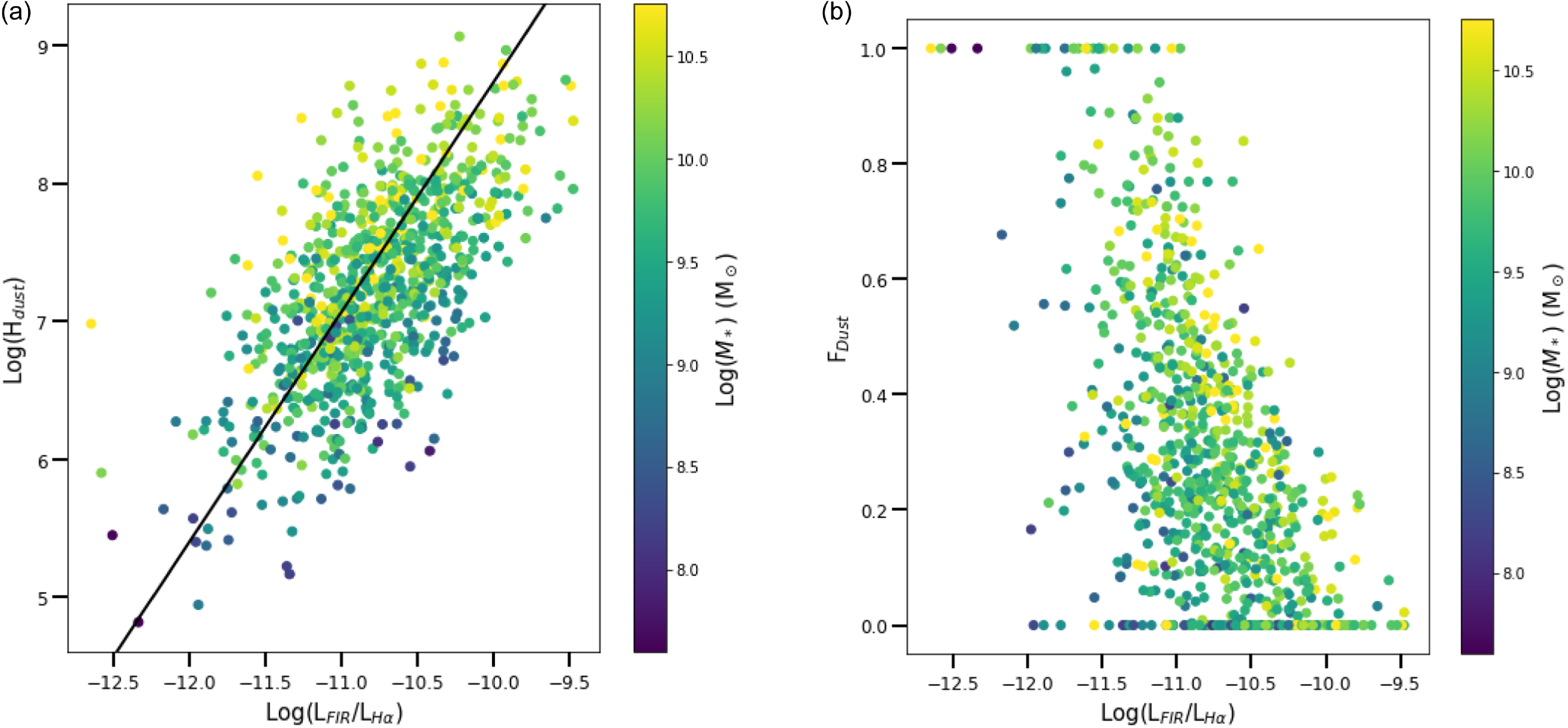
Figure 13 shows the relationship between $F_\textrm{dust}$
and
$F_\textrm{dust}$
and $H_\textrm{dust}$
with the H
$H_\textrm{dust}$
with the H $\alpha$
deficit for each of the four mass-limited redshift bins. The line in Figure 12a is not a fit, simply defined to guide the eye. This same line is overlayed onto each of the mass-limited redshift bins in Figure 13a. In each of these bins, while the sample becomes progressively limited to the higher
$\alpha$
deficit for each of the four mass-limited redshift bins. The line in Figure 12a is not a fit, simply defined to guide the eye. This same line is overlayed onto each of the mass-limited redshift bins in Figure 13a. In each of these bins, while the sample becomes progressively limited to the higher $M_*$
systems, the trend is consistent with the full sample. This demonstrates that the broad relationship between
$M_*$
systems, the trend is consistent with the full sample. This demonstrates that the broad relationship between $H_\textrm{ dust}$
and the H
$H_\textrm{ dust}$
and the H $\alpha$
deficit does not evolve over this redshift range.
$\alpha$
deficit does not evolve over this redshift range.
(a) $H_\textrm{dust}$
as a function of H
$H_\textrm{dust}$
as a function of H $\alpha$
deficit coloured by
$\alpha$
deficit coloured by $M_*$
for the mass-limited redshift bins, and (b)
$M_*$
for the mass-limited redshift bins, and (b) $F_\textrm{dust}$
as a function of H
$F_\textrm{dust}$
as a function of H $\alpha$
deficit coloured by
$\alpha$
deficit coloured by $M_*$
for the mass-limited redshift bins. The lines in (a) are the same as in Figure 12a to guide the eye, and highlight that, while the masses sampled in higher redshift bins increase, the galaxy population follows the same trend.
$M_*$
for the mass-limited redshift bins. The lines in (a) are the same as in Figure 12a to guide the eye, and highlight that, while the masses sampled in higher redshift bins increase, the galaxy population follows the same trend.
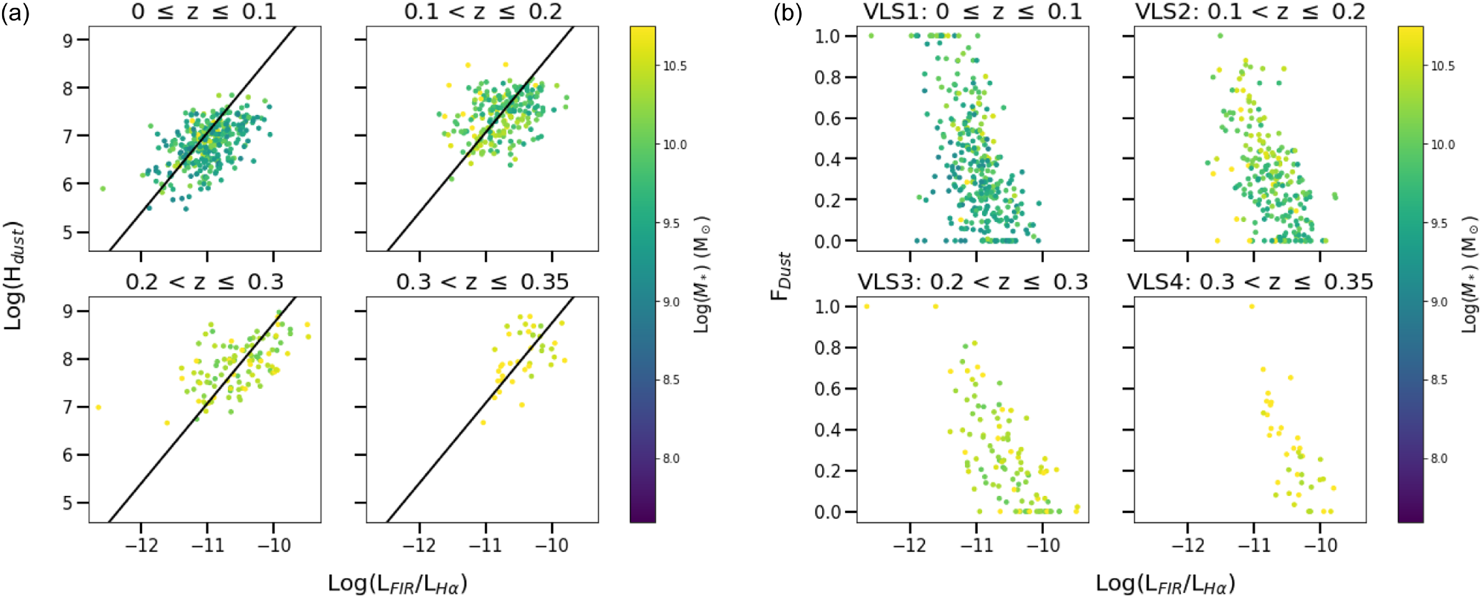
Figure 13b shows the relationship between $F_\textrm{dust}$
and the H
$F_\textrm{dust}$
and the H $\alpha$
deficit over the four redshift bins. Since each redshift bin samples galaxies limited to higher
$\alpha$
deficit over the four redshift bins. Since each redshift bin samples galaxies limited to higher $M_*$
, the mass dependence visible in Figure 12b is highlighted. As redshift increases, higher
$M_*$
, the mass dependence visible in Figure 12b is highlighted. As redshift increases, higher $M_*$
systems are selected. Accordingly, these correspond to galaxies with more distributed dust geometries and more optically thick dust. This is a consequence of selecting higher
$M_*$
systems are selected. Accordingly, these correspond to galaxies with more distributed dust geometries and more optically thick dust. This is a consequence of selecting higher $M_*$
galaxies at higher z, however, not any intrinsic evolutionary effect.
$M_*$
galaxies at higher z, however, not any intrinsic evolutionary effect.
We also explore the ratio between the FIR luminosity and the FUV luminosity which, analogous to the H $\alpha$
deficit, will be referred to here as the ‘FUV deficit’. Figure 14 shows the relationships between
$\alpha$
deficit, will be referred to here as the ‘FUV deficit’. Figure 14 shows the relationships between $H_\textrm{dust}$
and
$H_\textrm{dust}$
and $F_\textrm{dust}$
with the FUV deficit. The trends seen in this figure reiterate those seen in the corresponding H
$F_\textrm{dust}$
with the FUV deficit. The trends seen in this figure reiterate those seen in the corresponding H $\alpha$
deficit figures. Once again, higher FUV deficit values indicate a greater optical depth for the shorter wavelength light, corresponding to higher
$\alpha$
deficit figures. Once again, higher FUV deficit values indicate a greater optical depth for the shorter wavelength light, corresponding to higher $H_\textrm{dust}$
values and the distributed dust geometry of low values of
$H_\textrm{dust}$
values and the distributed dust geometry of low values of $F_\textrm{dust}$
.
$F_\textrm{dust}$
.
(a) $H_\textrm{dust}$
as a function of FUV deficit coloured by
$H_\textrm{dust}$
as a function of FUV deficit coloured by $M_*$
, and (b)
$M_*$
, and (b) $F_\textrm{dust}$
as a function of FUV deficit coloured by
$F_\textrm{dust}$
as a function of FUV deficit coloured by $M_*$
. The correlation coefficient for panel (a) is 0.52 and the correlation coefficient for panel (b) is −0.52.
$M_*$
. The correlation coefficient for panel (a) is 0.52 and the correlation coefficient for panel (b) is −0.52.
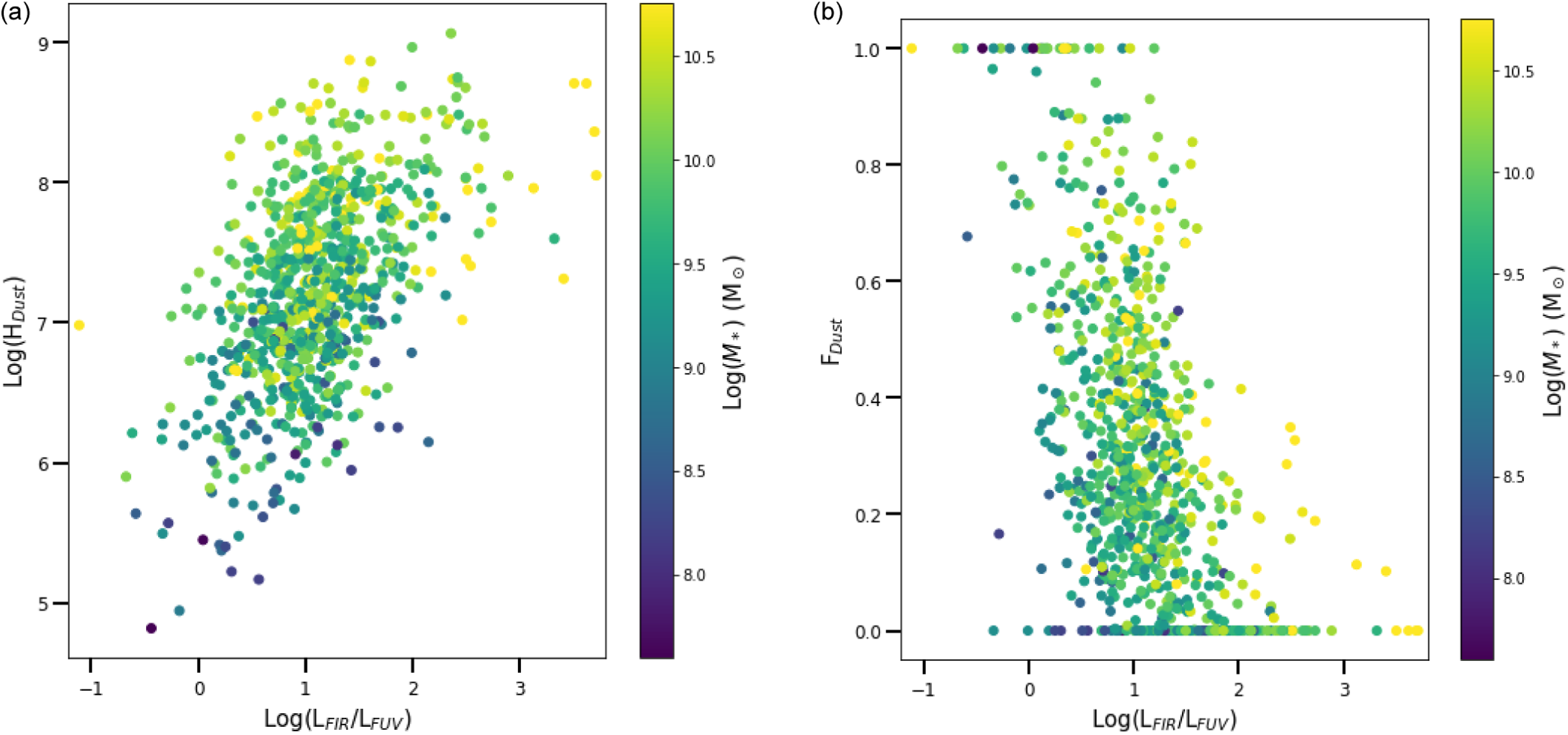
6. Discussion
We have established that $H_\textrm{dust}$
and
$H_\textrm{dust}$
and $F_\textrm{dust}$
appear to be sensitive to short wavelength deficits, which we attribute to a degree of optically thick obscuration. We can now use that result to explore how the dust geometry as traced by
$F_\textrm{dust}$
appear to be sensitive to short wavelength deficits, which we attribute to a degree of optically thick obscuration. We can now use that result to explore how the dust geometry as traced by $H_\textrm{dust}$
and
$H_\textrm{dust}$
and $F_\textrm{dust}$
varies for different galaxy properties. We look specifically at the relationship with galaxy stellar mass, SFR, and specific SFR.
$F_\textrm{dust}$
varies for different galaxy properties. We look specifically at the relationship with galaxy stellar mass, SFR, and specific SFR.
Figure 15 illustrates how $H_\textrm{dust}$
and
$H_\textrm{dust}$
and $F_\textrm{dust}$
vary with
$F_\textrm{dust}$
vary with $M_*$
. Figure 15a shows
$M_*$
. Figure 15a shows $H_\textrm{dust}$
increasing with stellar mass, which is to be expected given its strong link to the dust mass, and the correlation between dust mass and stellar mass. The SFR also clearly correlates with stellar mass, and, for a given SFR,
$H_\textrm{dust}$
increasing with stellar mass, which is to be expected given its strong link to the dust mass, and the correlation between dust mass and stellar mass. The SFR also clearly correlates with stellar mass, and, for a given SFR, $H_\textrm{dust}$
and stellar mass are strongly correlated. This implies that the most optically thick dust, at the highest values of
$H_\textrm{dust}$
and stellar mass are strongly correlated. This implies that the most optically thick dust, at the highest values of $H_\textrm{dust}$
, are, as might be expected, in the systems with both the highest stellar mass and the highest SFRs. The most extreme such systems (in the upper right, with the highest
$H_\textrm{dust}$
, are, as might be expected, in the systems with both the highest stellar mass and the highest SFRs. The most extreme such systems (in the upper right, with the highest $M_*$
) are likely absent from this diagram. This is due to the selection bias introduced by complete optically thick obscuration of the Balmer lines in the highest dust mass galaxies (corresponding to the absence of data in the upper right of Figure 2a).
$M_*$
) are likely absent from this diagram. This is due to the selection bias introduced by complete optically thick obscuration of the Balmer lines in the highest dust mass galaxies (corresponding to the absence of data in the upper right of Figure 2a).
The relationship between $M_*$
and (a)
$M_*$
and (a) $H_\textrm{dust}$
, and (b)
$H_\textrm{dust}$
, and (b) $F_\textrm{dust}$
coloured by SFR
$F_\textrm{dust}$
coloured by SFR $_{\text{H}\alpha}$
. The data are separated into four
$_{\text{H}\alpha}$
. The data are separated into four $M_*$
bins. The black stars represent the median value in each bin when the bins are evenly spaced. The black diamonds represent the median value in each bin when there are approximately the same number of objects in each bin. The errorbars show the median absolute deviations. The correlation coefficient for panel (a) is 0.50 and the correlation coefficient for panel (b) is 0.13.
$M_*$
bins. The black stars represent the median value in each bin when the bins are evenly spaced. The black diamonds represent the median value in each bin when there are approximately the same number of objects in each bin. The errorbars show the median absolute deviations. The correlation coefficient for panel (a) is 0.50 and the correlation coefficient for panel (b) is 0.13.
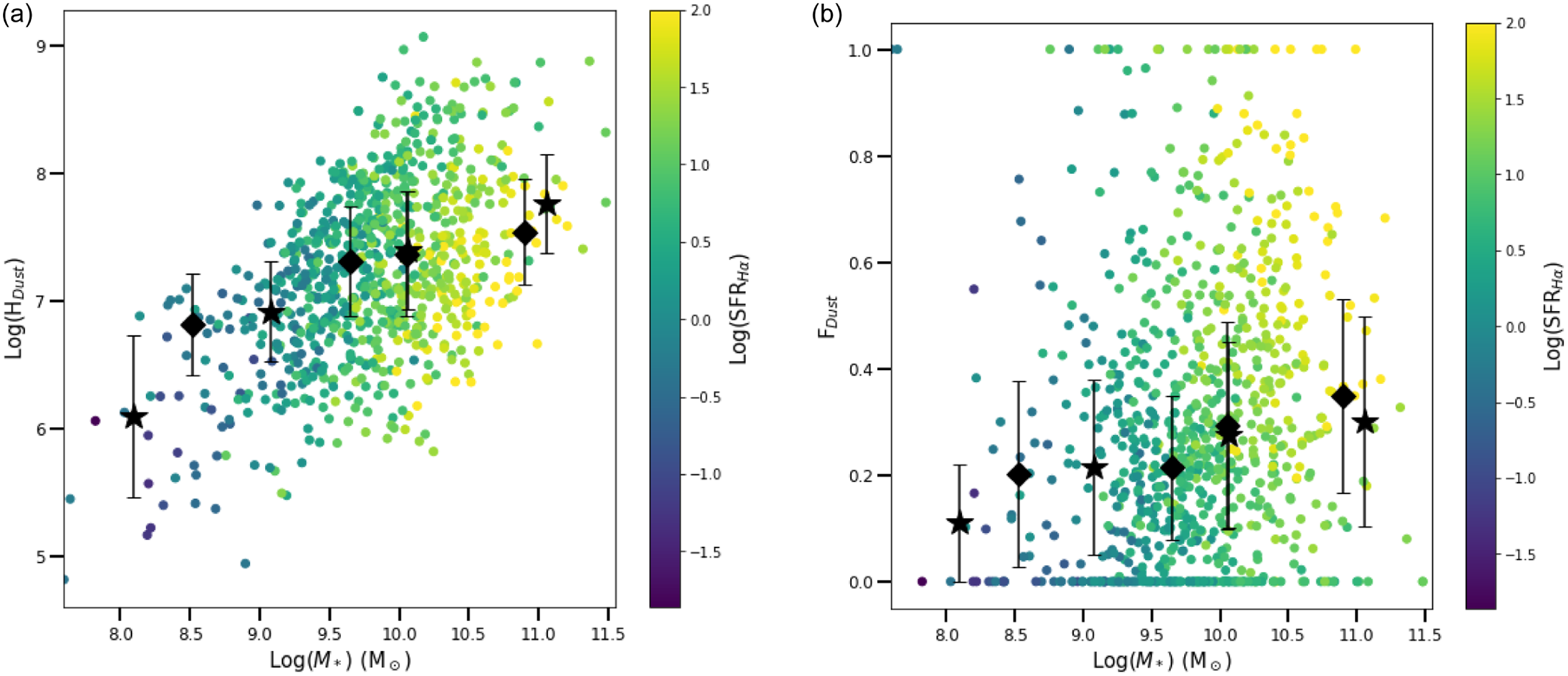
Figure 15b shows the relationship between $F_\textrm{dust}$
and stellar mass coloured by SFR
$F_\textrm{dust}$
and stellar mass coloured by SFR $_{\text{H}\alpha}$
. This figure shows a slight increase in the median
$_{\text{H}\alpha}$
. This figure shows a slight increase in the median $F_\textrm{dust}$
values with
$F_\textrm{dust}$
values with $M_*$
. The lack of a strong correlation between
$M_*$
. The lack of a strong correlation between $F_\textrm{ dust}$
and
$F_\textrm{ dust}$
and $M_*$
suggests that the proportion of foreground screen or distributed geometry present in a galaxy is not primarily influenced by the galaxy’s stellar mass. It can also be seen that at a given value of SFR
$M_*$
suggests that the proportion of foreground screen or distributed geometry present in a galaxy is not primarily influenced by the galaxy’s stellar mass. It can also be seen that at a given value of SFR $_{\text{H}\alpha}$
,
$_{\text{H}\alpha}$
, $F_\textrm{ dust}$
decreases as
$F_\textrm{ dust}$
decreases as $M_*$
increases (a slightly inverse correlation at fixed SFR). This indicates that for a given SFR, a lower mass galaxy will favour a more foreground screen geometry, while a higher mass galaxy will show a more distributed dust geometry.
$M_*$
increases (a slightly inverse correlation at fixed SFR). This indicates that for a given SFR, a lower mass galaxy will favour a more foreground screen geometry, while a higher mass galaxy will show a more distributed dust geometry.
Figure 16 presents the dependence of $H_\textrm{dust}$
and
$H_\textrm{dust}$
and $F_\textrm{dust}$
on SFR
$F_\textrm{dust}$
on SFR $_{\text{H}\alpha}$
. Figure 16b shows a positive trend between
$_{\text{H}\alpha}$
. Figure 16b shows a positive trend between $H_\textrm{dust}$
and SFR
$H_\textrm{dust}$
and SFR $_{\text{H}\alpha}$
, which then flattens and turns downwards at the highest values of SFR
$_{\text{H}\alpha}$
, which then flattens and turns downwards at the highest values of SFR $_{\text{H}\alpha}$
. This is attributable to the absence of the highest
$_{\text{H}\alpha}$
. This is attributable to the absence of the highest $H_\textrm{dust}$
values. Again, this absence of data points in the high
$H_\textrm{dust}$
values. Again, this absence of data points in the high $H_\textrm{dust}$
, high SFR, high
$H_\textrm{dust}$
, high SFR, high $M_*$
region can be attributed to the selection bias from the complete obscuration of the Balmer lines. At a given
$M_*$
region can be attributed to the selection bias from the complete obscuration of the Balmer lines. At a given $M_*$
,
$M_*$
, $H_\textrm{dust}$
decreases with increasing SFR
$H_\textrm{dust}$
decreases with increasing SFR $_{\text{H}\alpha}$
. This indicates that for galaxies of a given mass, higher SFRs occur in those with less optically thick dust.
$_{\text{H}\alpha}$
. This indicates that for galaxies of a given mass, higher SFRs occur in those with less optically thick dust.
The relationship between SFR $_{\text{H}\alpha}$
and (a)
$_{\text{H}\alpha}$
and (a) $H_\textrm{dust}$
, and (b)
$H_\textrm{dust}$
, and (b) $F_\textrm{dust}$
coloured by
$F_\textrm{dust}$
coloured by $M_*$
. The data are separated into four SFR bins. The black stars represent the median value in each bin when the bins are evenly spaced. The black diamonds represent the median value in each bin when there are approximately the same number of objects in each bin. The errorbars show the median absolute deviations. If the errorbars are not visible, it is because they are smaller than the star markers. The correlation coefficient for panel (a) is 0.26 and the correlation coefficient for panel (b) is 0.49.
$M_*$
. The data are separated into four SFR bins. The black stars represent the median value in each bin when the bins are evenly spaced. The black diamonds represent the median value in each bin when there are approximately the same number of objects in each bin. The errorbars show the median absolute deviations. If the errorbars are not visible, it is because they are smaller than the star markers. The correlation coefficient for panel (a) is 0.26 and the correlation coefficient for panel (b) is 0.49.
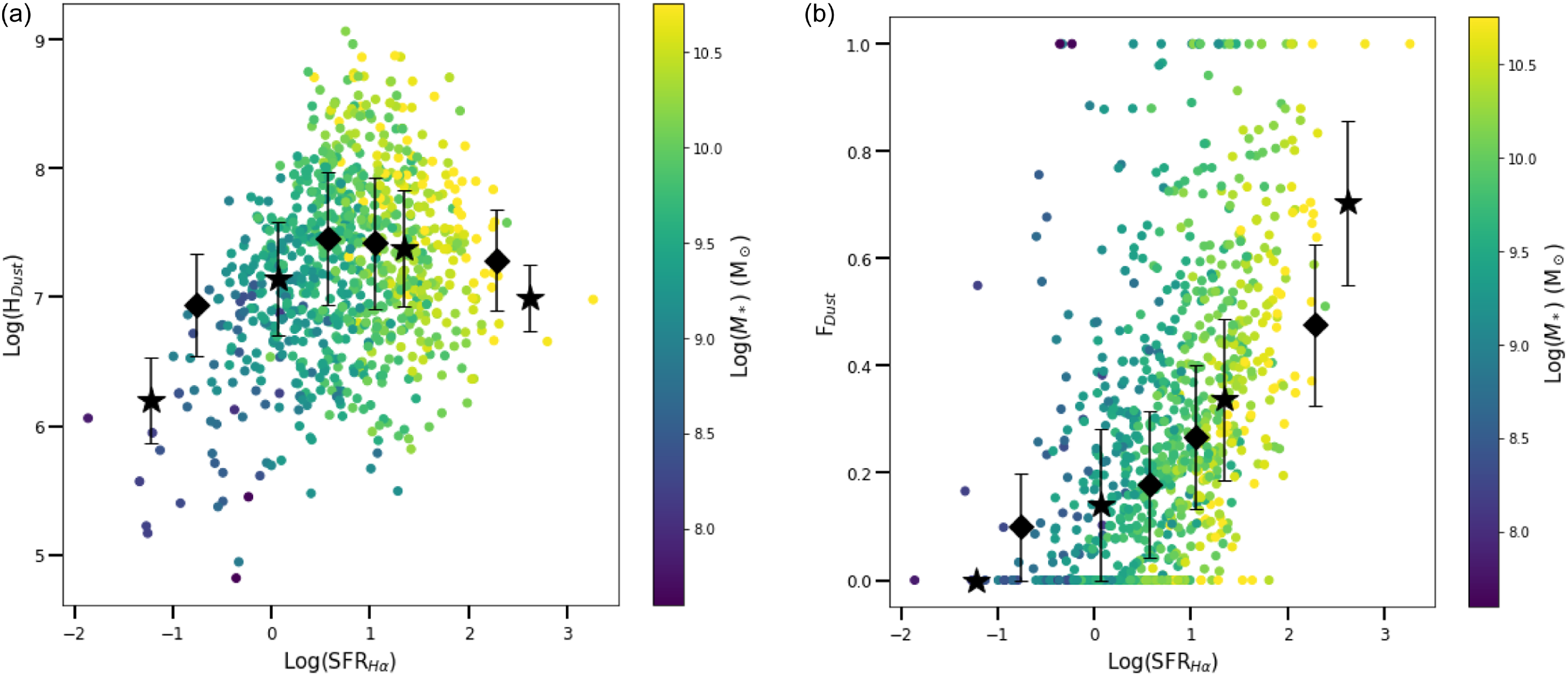
 $F_\textrm{dust}$
is clearly correlated with SFR
$F_\textrm{dust}$
is clearly correlated with SFR $_{\text{H}\alpha}$
, as seen in Figure 16b. The influence of
$_{\text{H}\alpha}$
, as seen in Figure 16b. The influence of $M_*$
in this figure can also be seen. The strong
$M_*$
in this figure can also be seen. The strong $M_*$
-SFR
$M_*$
-SFR $_{\text{H}\alpha}$
relationship is visible, but equally clear is that for a fixed
$_{\text{H}\alpha}$
relationship is visible, but equally clear is that for a fixed $M_*$
a strong positive correlation exists between
$M_*$
a strong positive correlation exists between $F_\textrm{dust}$
and SFR
$F_\textrm{dust}$
and SFR $_{\text{H}\alpha}$
. This indicates that the proportion of foreground screen contribution to the dust geometry increases as SFR
$_{\text{H}\alpha}$
. This indicates that the proportion of foreground screen contribution to the dust geometry increases as SFR $_{\text{H}\alpha}$
increases.
$_{\text{H}\alpha}$
increases.
The negative correlation between $H_\textrm{dust}$
and
$H_\textrm{dust}$
and $F_\textrm{dust}$
can be seen in Figure 16 in the
$F_\textrm{dust}$
can be seen in Figure 16 in the $M_*$
dependence in each panel. In both the broad trend between
$M_*$
dependence in each panel. In both the broad trend between $M_*$
and SFR is apparent. However, in 16b, at a fixed
$M_*$
and SFR is apparent. However, in 16b, at a fixed $M_*$
$M_*$ $H_\textrm{dust}$
decreases with SFR
$H_\textrm{dust}$
decreases with SFR $_{\text{H}\alpha}$
, while in 16a at a fixed
$_{\text{H}\alpha}$
, while in 16a at a fixed $M_*$
$M_*$ $F_\textrm{dust}$
increases with SFR
$F_\textrm{dust}$
increases with SFR $_{\text{H}\alpha}$
.
$_{\text{H}\alpha}$
.
Figure 17 rounds out the collection by showing how $H_\textrm{dust}$
and
$H_\textrm{dust}$
and $F_\textrm{dust}$
depend on sSFR
$F_\textrm{dust}$
depend on sSFR $_{\text{H}\alpha}$
. Figure 17a shows the relationship for
$_{\text{H}\alpha}$
. Figure 17a shows the relationship for $H_\textrm{dust}$
. Here, the median values show
$H_\textrm{dust}$
. Here, the median values show $H_\textrm{dust}$
decreasing as sSFR increases. This trend of
$H_\textrm{dust}$
decreasing as sSFR increases. This trend of $H_\textrm{dust}$
decreasing as sSFR increases is consistent with Figure 16a in which, for a given
$H_\textrm{dust}$
decreasing as sSFR increases is consistent with Figure 16a in which, for a given $M_*$
,
$M_*$
, $H_\textrm{dust}$
decreases with increasing SFR
$H_\textrm{dust}$
decreases with increasing SFR $_{\text{H}\alpha}$
. The
$_{\text{H}\alpha}$
. The $M_*$
colour coding shows how the use of sSFR has removed much of the stellar mass dependence seen in Figure 16a.
$M_*$
colour coding shows how the use of sSFR has removed much of the stellar mass dependence seen in Figure 16a.
The relationship between sSFR $_{\text{H}\alpha}$
and (a)
$_{\text{H}\alpha}$
and (a) $H_\textrm{dust}$
, and (b)
$H_\textrm{dust}$
, and (b) $F_\textrm{dust}$
, coloured by
$F_\textrm{dust}$
, coloured by $M_*$
. The data are separated into four sSFR bins. The black stars represent the median value in each bin when the bins are evenly spaced. The black diamonds represent the median value in each bin when there are approximately the same number of objects in each bin. The errorbars show the median absolute deviations. If the errorbars are not visible, it is because they are smaller than the star markers. The correlation coefficient for panel (a) is −0.28 and the correlation coefficient for panel (b) 0.596.
$M_*$
. The data are separated into four sSFR bins. The black stars represent the median value in each bin when the bins are evenly spaced. The black diamonds represent the median value in each bin when there are approximately the same number of objects in each bin. The errorbars show the median absolute deviations. If the errorbars are not visible, it is because they are smaller than the star markers. The correlation coefficient for panel (a) is −0.28 and the correlation coefficient for panel (b) 0.596.
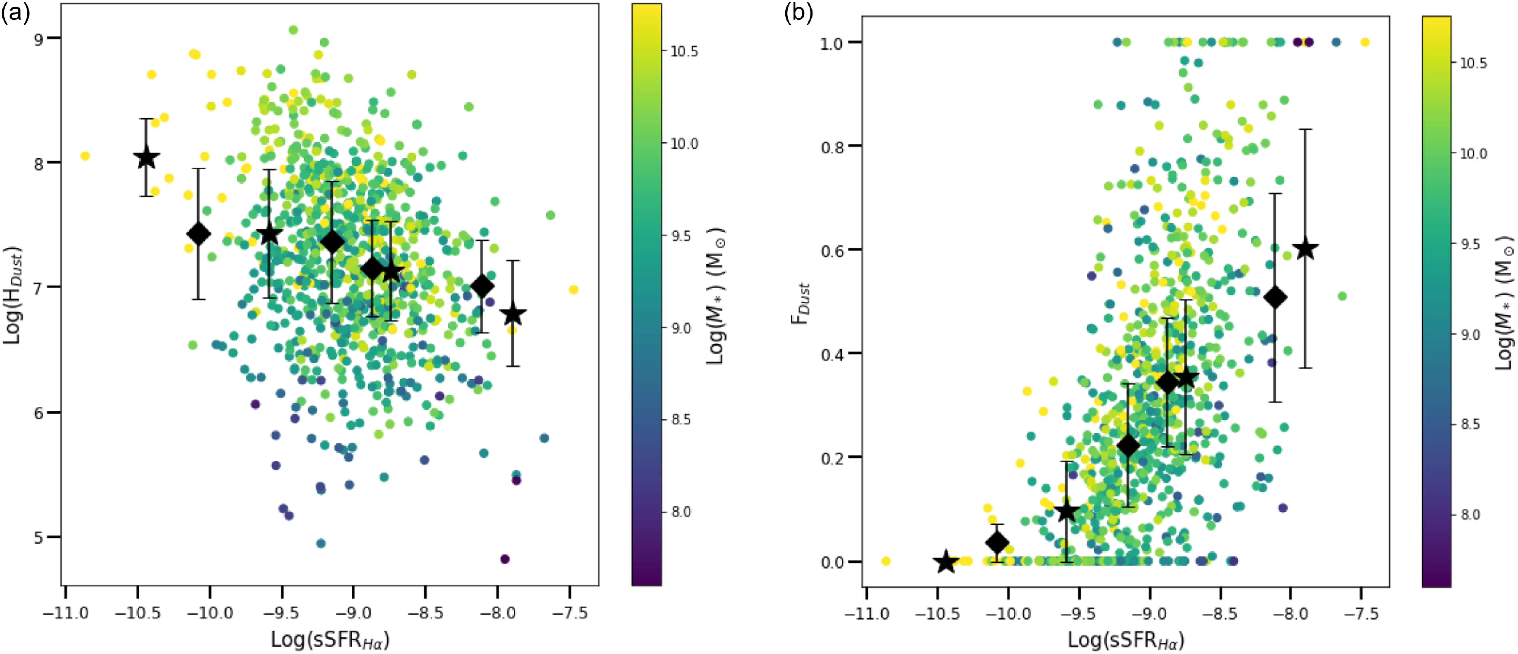
Figure 17b shows the correlation between $F_\textrm{dust}$
and sSFR
$F_\textrm{dust}$
and sSFR $_{\text{H}\alpha}$
. The use of sSFR removes the
$_{\text{H}\alpha}$
. The use of sSFR removes the $M_*$
dependence visible in Figure 16b, demonstrating that the contribution of foreground screen dust to the geometry clearly increases with an increase in H
$M_*$
dependence visible in Figure 16b, demonstrating that the contribution of foreground screen dust to the geometry clearly increases with an increase in H $\alpha$
star formation intensity. Galaxies with high sSFR and high
$\alpha$
star formation intensity. Galaxies with high sSFR and high $F_\textrm{dust}$
can clearly be associated with the maximal foreground screen dust geometry. Conversely, galaxies with low sSFR correspond to a more distributed dust geometry.
$F_\textrm{dust}$
can clearly be associated with the maximal foreground screen dust geometry. Conversely, galaxies with low sSFR correspond to a more distributed dust geometry.
Taken together, these results can be interpreted as confirming that galaxies with high SFR and sSFR are best characterised with a ‘maximal foreground screen’ dust geometry. This is consistent with the widely adopted choice of dust model for starburst galaxies (e.g., Calzetti, Kinney, & Storchi-Bergmann Reference Calzetti, Kinney and Storchi-Bergmann1994; Calzetti et al. Reference Calzetti, Armus, Bohlin, Kinney, Koornneef and Storchi-Bergmann2000, Reference Calzetti2001a). Conversely, galaxies with low SFR and sSFR appear to strongly favour the ‘maximal distributed dust’ geometry. They also demonstrated the least optically thick dust, evidenced in their low values of $H_\textrm{dust}$
, while the high SFR and high mass systems contain a greater degree of optically thick dust. The systems with the highest values of
$H_\textrm{dust}$
, while the high SFR and high mass systems contain a greater degree of optically thick dust. The systems with the highest values of $H_\textrm{dust}$
are also those with the highest masses and lowest sSFR.
$H_\textrm{dust}$
are also those with the highest masses and lowest sSFR.
Ahmed et al. (in preparation) continue to explore the use of $F_\textrm{dust}$
and
$F_\textrm{dust}$
and $H_\textrm{dust}$
by incorporating radio luminosities in their analysis. The use of the longer wavelength radio luminosity, which is not sensitive to obscuration, allows for an independent comparison to the results seen here when using the H
$H_\textrm{dust}$
by incorporating radio luminosities in their analysis. The use of the longer wavelength radio luminosity, which is not sensitive to obscuration, allows for an independent comparison to the results seen here when using the H $\alpha$
luminosity. Comparison of the trends seen when using a wavelength that is susceptible to obscuration with one that is not will help illuminate which trends observed in this paper, if any, may be a consequence of the remaining loss of H
$\alpha$
luminosity. Comparison of the trends seen when using a wavelength that is susceptible to obscuration with one that is not will help illuminate which trends observed in this paper, if any, may be a consequence of the remaining loss of H $\alpha$
emission due to obscuration.
$\alpha$
emission due to obscuration.
7. Conclusion
We have introduced two new parameters, $H_\textrm{dust}$
and
$H_\textrm{dust}$
and $F_\textrm{dust}$
that provide a novel method to quantify the properties of obscuration in galaxies. These parameters both use the BD and dust mass combined to infer more information about dust geometry and optical depth. We explored the use of dust surface density in place of dust mass in these parameters. Dust mass was demonstrated to be the more robust and effective approach in the definition of these new dust parameters. We have demonstrated that the BD and dust mass are explicitly linked to the degree of optically thick obscuration by comparison to parameters quantifying an H
$F_\textrm{dust}$
that provide a novel method to quantify the properties of obscuration in galaxies. These parameters both use the BD and dust mass combined to infer more information about dust geometry and optical depth. We explored the use of dust surface density in place of dust mass in these parameters. Dust mass was demonstrated to be the more robust and effective approach in the definition of these new dust parameters. We have demonstrated that the BD and dust mass are explicitly linked to the degree of optically thick obscuration by comparison to parameters quantifying an H $\alpha$
or UV deficit (
$\alpha$
or UV deficit ( $L_\textrm{FIR}/L_{\text{H}\alpha}$
or
$L_\textrm{FIR}/L_{\text{H}\alpha}$
or $L_\textrm{FIR}/L_{\text{FUV}}$
). We show that
$L_\textrm{FIR}/L_{\text{FUV}}$
). We show that $H_\textrm{dust}$
is a good tracer for the degree of optically thick dust in a galaxy, and that
$H_\textrm{dust}$
is a good tracer for the degree of optically thick dust in a galaxy, and that $F_\textrm{dust}$
is an efficient parameter to quantify the form of the dust geometry.
$F_\textrm{dust}$
is an efficient parameter to quantify the form of the dust geometry.
We use these parameters to explore how dust opacity and geometry relate to other basic galaxy properties. We see that $F_\textrm{dust}$
has no dependence on stellar mass, due to the nature of how it is defined, but
$F_\textrm{dust}$
has no dependence on stellar mass, due to the nature of how it is defined, but $H_\textrm{dust}$
does correlate with
$H_\textrm{dust}$
does correlate with $M_*$
(Figure 15), as a consequence of its link with dust mass by definition. However, its ability to quantify the optical depth is not stellar mass dependent, and the range of optical depth sampled (the range of
$M_*$
(Figure 15), as a consequence of its link with dust mass by definition. However, its ability to quantify the optical depth is not stellar mass dependent, and the range of optical depth sampled (the range of $H_\textrm{dust}$
values) becomes larger at higher
$H_\textrm{dust}$
values) becomes larger at higher $M_*$
.
$M_*$
.
We have also shown that these parameters are linked to SFR and sSFR. It is clear that the assumption of a maximal foreground screen dust model is appropriate for highly star forming galaxies, when measuring obscuration-sensitive properties such as H $\alpha$
(Figs. 16b and 17b). It is also the case that the highest SFR galaxies show the greatest level of optical depth (Figure 16a), even while these may be low sSFR systems given their large
$\alpha$
(Figs. 16b and 17b). It is also the case that the highest SFR galaxies show the greatest level of optical depth (Figure 16a), even while these may be low sSFR systems given their large $M_*$
(Figure 17a). Together this implies that in the highest SFR systems there is likely to be a deficit in the measured H
$M_*$
(Figure 17a). Together this implies that in the highest SFR systems there is likely to be a deficit in the measured H $\alpha$
, even after obscuration correction, due to optically thick dust.
$\alpha$
, even after obscuration correction, due to optically thick dust.
The ability to measure dust geometry and have a quantitative constraint on the degree of optically thick dust opens many possibilities for better measurement and understanding of fundamental galaxy properties. Future work will investigate dependencies on metallicity, inclination, morphology, environment, redshift, and other galaxy properties. Quantifying a series of models encompassing all geometries may also provide a fruitful direction for future work. We will also explore whether there are further refinements in how we may define $H_\textrm{dust}$
and
$H_\textrm{dust}$
and $F_\textrm{dust}$
, or incorporate other properties to provide still better insights into the dust properties of galaxies.
$F_\textrm{dust}$
, or incorporate other properties to provide still better insights into the dust properties of galaxies.
Acknowledgement
GAMA is a joint European-Australasian project based around a spectroscopic campaign using the Anglo-Australian Telescope. The GAMA input catalogue is based on data taken from the Sloan Digital Sky Survey and the UKIRT Infrared Deep Sky Survey. Complementary imaging of the GAMA regions is being obtained by a number of independent survey programmes including GALEX MIS, VST KiDS, VISTA VIKING, WISE, Herschel-ATLAS, GMRT and ASKAP providing UV to radio coverage. GAMA is funded by the STFC (UK), the ARC (Australia), the AAO, and the participating institutions. The GAMA website is http://www.gama-survey.org/. Based on observations made with ESO Telescopes at the La Silla Paranal Observatory under programme IDs 179.A-2004 and 177.A-3016.
Data availability statement
The GAMA data are all publicly available.Footnote a


 Open access