Introduction
Due to current warming climatic conditions, most Swiss glaciers are retreating drastically (Glaciological reports, 1881-2009). These changes have given rise to the formation of proglacial lakes or subglacial water pockets, which can lead to outburst events (e.g. Reference SolomonSolomon and others, 2007). In addition, glacier tongues can become unstable as glaciers retreat into steeper terrain (Reference ROthlisberger and KasserRothlisberger and Kasser, 1978). According to the inventory of hazardous glaciers in Switzerland (Reference Raymond, Wegmann and FunkRaymond and others, 2003), 82 glacierized places are recognized as dangerous, and statistics show that a damaging event has occurred every 20 years. In the case of unstable glacier tongues or hanging glaciers, falling ice can trigger snow avalanches or the outburst of glacial lakes. Hazard mitigation measures may require forecasting of such an event at a daily timescale.
Two types of glacier instabilities exist, mechanical and sliding. The first type arises in the case of cold ramp glaciers frozen to the glacier bed, where snow accumulation is mostly compensated with break-off (Faillettaz and others, 2007). A typical example is Weisshorn hanging glacier, Switzerland, which is known for periodic break-off events (Reference FlotronFlotron, 1977; Reference Rothlisberger, Kasser and HaeberliRothlisberger, 1981a; Reference Raymond, Wegmann and FunkRaymond and others, 2003; Reference Pralong and FunkPralong and Funk, 2006; Reference Faillettaz, Pralong, Funk and DeichmannFaillettaz and others, 2008). If a break-off event occurs in winter, the icefall may trigger a large combined snow/ice avalanche, which constitutes a serious threat to the village of Randa in Mattertal, located downstream from Weisshorngletscher. In order to bring to light precursors of such an event, passive seismic and surface displacement surveys were performed in 2005 (Reference Faillettaz, Pralong, Funk and DeichmannFaillettaz and others, 2008). The authors highlighted a log-periodic power- law acceleration of the surface motion before the break- off. They also established a correlation between seismic activity and the imminence of the break-off event. By combining both observations, they demonstrated that during the initiation of the instability, prediction of the time of break-off could be improved significantly (Reference Faillettaz, Funk and SornetteFaillettaz and others, 2011). Seismic characteristics during the maturation process of an icefall were also surveyed by Reference Caplan-Auerbach and HuggelCaplan-Auerbach and Huggel (2007) on Iliamna volcano, Alaska, USA. They analysed the seismic activity in the hours preceding break- off events and distinguished two precursory phases: first, a period of repeated seismic events, interpreted as slips at the bedrock interface or between layers of ice, and second, a phase of constant ground-shaking, corresponding to the accommodation of the slip through the deformation of the ice. They suggested this sequence could be used as a warning indicator for ice avalanche events.
The second type of glacier instability (sliding) may occur in the case of a steep temperate glacier tongue, where subglacial water pressure may substantially enhance basal motion, and, in certain cases, a large part of the glacier tongue may become unstable (Reference RothlisbergerRothlisberger, 1987). Such an event occurred on Allalingletscher, Saastal, Switzerland, in 1965, where the main part of the tongue broke off and devastated the construction site of the Mattmark dam, killing 88 people. Surface motion measurements began just after the event and were pursued in the following years (Reference ROthlisberger and KasserRothlisberger and Kasser, 1978). Characteristic periods of increasing velocity called ‘active phases’ were detected almost every year, mostly during summer. However, they were only followed twice by a large-extent break-off episode (Reference Rothlisberger, Kasser and HaeberliRothlisberger, 1981b), indicating that surface motion alone cannot be used as a precursor. In this context and given the encouraging results obtained for mechanical instabilities (Reference Faillettaz, Pralong, Funk and DeichmannFaillettaz and others, 2008, Reference Faillettaz, Funk and Sornette2011), seismic monitoringseems to be a promising complementary tool for characterizing changes in the dynamics of steep temperate glacier tongues which can lead to large-scale break-offs.
Several studies have shown that glaciers can generate seismic signals called icequakes. In the case of serac falls located in temperate glaciers, three main seismic sources can be discerned: (1) the brittle deformation of ice, (2) glacier basal motion and (3) basal hydrology. In case (1) Reference Neave and SavageNeave and Savage (1970) associated high-frequency seismic events on Athabasca Glacier, Canada, with the opening of surface crevasses. A recent study on Columbia Glacier, Alaska, by Reference O’Neel, Marshall, McNamara and PfefferO’Neel and others (2007) reported analogous results,with icequakes lying within a 10-20 Hz band. The second source of seismicity (2) was first documented by Reference Weaver and MaloneWeaver and Malone (1979), who found low-frequency seismic events that could be related to basal processes such as stick-slip sliding. Reference Deichmann, Ansorge, Scherbaum, Aschwanden, Bernardi and GudmundssonDeichmann and others (2000) confirmed that icequakes could occur at any depth, including near the bedrock. Reference Walter, Deichmann and FunkWalter and others (2008) studied the seismic activity of Gornergletscher, Switzerland, during the summers of 200406, as subglacial water pressure varied drastically during the drainage of a glacier-dammed lake. They detected several thousands of seismic signals per day and located ~200 events near the glacier bed. They explained the basal icequake activity by variations in basal motion caused by water-pressure fluctuations. In this case, deep icequakes seemed to be caused by tensile fracturing near the glacier bed. The third type of seismic event (3) was mentioned by Reference Lawrence and QamarLawrence and Quamar (1979). They proposed a hydraulic origin for a 1-5 Hz seismic signal exhibiting emergent onset and no clear distinction between compression and shear waves. They demonstrated that such events were triggered by displacement of water-filled subglacial conduits. Reference Metaxian, Araujo, Mora and LesageMetaxian and others (2003) investigated icequakes detected on the glacier of Cotopaxi volcano, Ecuador. They interpreted the signals as resonance of water-filled ice cavities, which may be activated by ice cracking or sudden changes in water flow at the glacier base. However, such signals were also observed in volcanic regions, where the interaction between magma and groundwater is likely to lead to vibrations in fluid- filled cracks (Reference Chouet, Page, Stephens, Lahr and PowerChouet and others, 1994). Seismic emissions associated with a glacier surge have also been observed in Spitsbergen, Svalbard (Reference Stuart, Murray, Brisbourne, Styles and ToonStuart and others, 2005). The authors related them to specific basal icequakes and water-filled cracks close to the glacier bed. The seismic activity can also be caused by interaction between several sources.
This work presents an analysis of the potential interactions between seismic activity, surface motion and subglacial water drainage in the steep part of the temperate Triftgletscher (Fig. 1 a and b) during summer 2008. The goal is to explore the seismic response of the glacier to its dynamics, to assess the different sources of the microseismic activity emitted by the glacier and to identify possible break-off precursors. The paper is organized as follows: The method employed to assess both surface motion and hourly runoff is first described and the associated results are presented. Then the seismic data processing is detailed and the spatial distribution of the observed seismic activity is discussed. A study of the content of the background noise and of its influence on the temporal distribution of the seismic activity follows. Finally, the influence of runoff changes on surface motion on a timescale of several days is studied and a statistical analysis of the released seismic energy is detailed. Some clues which may forecast a break-off are then discussed.
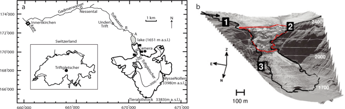
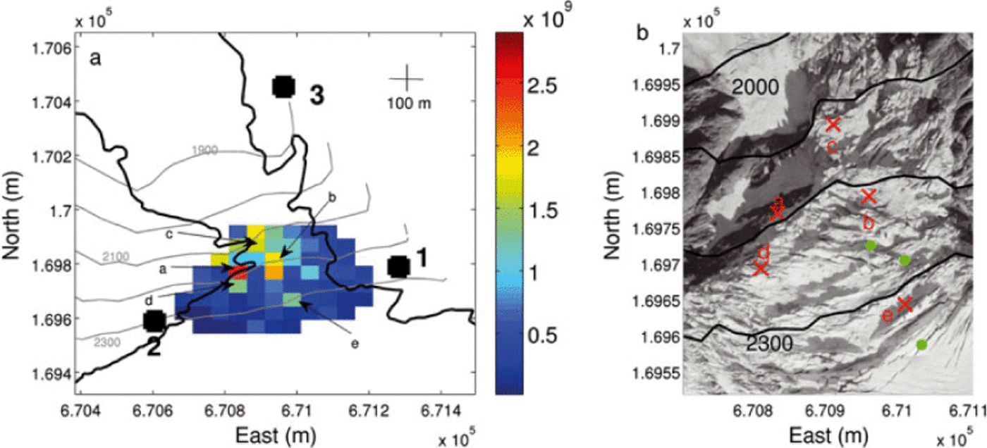
(a) Location and situation map of Triftgietscher: the three black squares are the seismic stations; the black circle represents the automatic camera; coordinates are expressed in the Swiss coordinate system (CH1903). (b) Frontal view of the Triftgietscher tongue in August 2008: black squares represent the three seismic stations; the black arrow close to station 1 indicates the automatic camera angle view; the red line marks the boundary of the zone investigated in the seismic survey; the thick black line illustrates the boundary of the englaciated area.
Study Site and Problem Definition
Triftgletscher is located between the Gadmer and Hasli valleys in the Bernese Alps, Switzerland (Fig. 1a). It has a length of 5.1 km, an area of 15 km2 and its altitude ranges between 3380 and 1651 ma.s.l. Between 2350 and 2050ma.s.l, it flows over a 35° steep section towards the flat tongue. The glacier snout lies in a basin, which is bordered on the north side by a riegel. The water drains out of the basin through a narrow canyon, deeply incised into the riegel. Over the last 15 years, Triftgletscher has retreated substantially from the riegel, forming a proglacial lake containing 5 × 10⁶m3 of water (R. Grischott and others, unpublished information). Because of the glacier retreat, and the thinning of the lower tongue, the stability of the steep section behind it is affected, increasing the likelihood of large ice avalanches from the steep section. The recent intensive glacier thinning in the lower tongue area (6-10ma-1; Reference MullerMuller, 2004) has further aggravated the situation, as the run-out path of the ice avalanches has become steeper. An avalanche dynamic and a hydraulic study have shown that ice avalanches with >106 m3 of ice can generate dangerous flood waves, threatening the safety of the inhabitants of the downstream Gadmertal valley (Reference Dalban CanassyDalban Canassy and others, 2011).
Surface Motion Computation by Photographic Analysis
Surface motion in the steep part of Triftgletscher was documented with the aid of a two-dimensional (2-D) photographic analysis, using pairs of consecutive photographs. The pictures were taken every 3 hours with an automatic camera (Nikon D200) installed in the vicinity of the Trifthutte (2580 m a.s.l.; Fig. 1a). The resolution was 3872 × 2592 pixels and they offer a view ranging from ~400 m upstream of the steep part to 100 m behind the end of the terminus. In this procedure, consecutive images (p1 and p2) were gridded and a greyscale correlation applied. For each gridpoint, a 2-D vector was obtained where the x- and y-coordinates referred to the two components of the horizontal displacement. Reference Dalban CanassyDalban Canassy and others (2011) provide further details, and found peak surface velocities ranging from 0.6 to 1.1 md-1 in summer and 0.4 md-1 during the rest of the year. Given that one pixel corresponded in situ to ~30cm and that the results accuracy was 0.1 pixel, the greyscale analysis was accurate enough to compute daily surface motion all year.
Due to technical problems, continuous photographs were available for two periods only, from 11 July to 8 August and from 20 August to 7 September. Moreover, because of the presence of snow on the objective lens of the camera, some pictures were unusable in mid-July. Photographs were taken five times a day, at 08:00, 11:00, 14:00, 17:00 and 20:00 local time. In the following, each shot is associated with the absolute time, ti . Surface motion calculations were performed using pairs of photographs taken at times ti and ti + 24 hours Fig. 2). In order to obtain data on the temporal evolution of surface motion, all the consecutive pairs of photographs time-spaced <24 hours apart (i.e. ti +1 — ti < 24 hours) were selected, and the displacements associated with interval Δ t,t i +24h were computed. The time associated with a given time interval was the mean value of both limits (black crosses in Fig. 2). As we chose t i+1 — ti < 24 hours, a 3 hour overlap between consecutive periods was possible.
Description of the method to determine surface motion. The computations were performed with pairs of photographs taken at absolute times ti and ti + 24 hours, with t i+1 — ti ≤ 24 hours. Black crosses stand for the middle of each interval and were chosen to mark them in the analysis. Note that a 3 hour overlap is possible from one pair to the next.
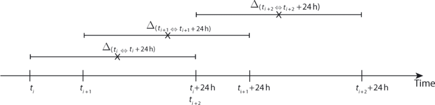
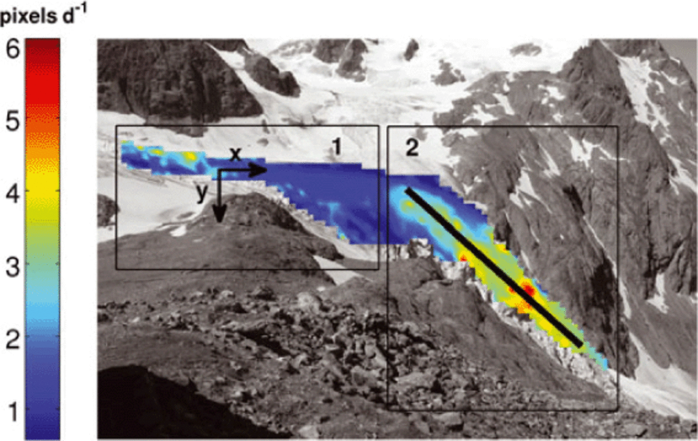
Figure 3 shows the mean daily surface displacements from 11 July to 8 August in the lower part of the glacier, for all the points on the mesh grid. Displayed values correspond to the norm of the two-component motion vector (black arrows x and y in Fig. 3) computed for every point. The size of each pixel varies according to its distance from the camera. For this reason, we decided to keep results in pixels d-1 and assumed that pixel size variation for the studied area is not significant with respect to the observed changes in surface motion. The surface displacement distribution reveals two distinct zones (frames 1 and 2 in Fig. 3). Zone 1 is upstream of the serac fall and indicates velocities ranging from 1 to 4 pixelsd-1. These values characterize the almost completely flat area. Zone 2 starts where the glacier becomes steeper and exhibits velocities greater than 3 pixels d-1. The break of the slope is clearly emphasized by a sudden motion increase, and the largest values (5 pixelsd-1) are found in the middle of the serac fall. Most of the velocities are close to 3.5 pixelsd-1, which corresponds to the results of Reference Dalban CanassyDalban Canassy and others (2011) for summer motion, taking a rough pixel size of 30 cm. Note that on the left side of the glacier, the vertical angle between the camera and the ice is too small and the pixel analysis becomes inaccurate. This may explain the very small values (<0.5 pixel d-1). In the next section, the glacial hydrology affecting the serac fall area is discussed.
Mean daily surface motion (pixels d−1) from 11 July to 8 August. The black line represents the flowline used for computations in comparison with the modelled runoff. The two rectangular frames, 1 and 2, correspond to the two areas referred to in themean daily motion analysis. Arrows labelled x and y represent the components of a resulting 2-D vector motion.
Runoff Data
The subglacial water flow affects the dynamics of the glacier (Reference IkenIken, 1981), and the emitted seismic activity is expected to reflect these changes. For our study period, daily discharges, recorded at a gauging station 2 km downstream of the lake, were available from the hydroelectric company KWO (KraftWerke Oberhasli, Switzerland). Water supply from smaller streams between the glacier tongue and the discharge record station was neglected. Based on these data, we modelled hourly runoff for the entire catchment above the icefall, whose surface area is 19.1 km2. We used a temperature-index melt model (Reference HockHock, 1999), based on a linear relation between melt rate and positive air temperature (Reference OhmuraOhmura, 2001). The model was run on a grid of 25 × 25 m, as described by Reference Huss, Farinotti, Bauder and FunkHuss and others (2008a, Reference Huss, Usselmann, Farinotti and Bauder2010) and Farinotti and others (in press). Runoff was inferred from liquid precipitation and ice and snow ablation. Snow and rainfall were distinguished with the help of a threshold temperature. Ablation was assessed at any gridcell, i, including the effect of the solar radiation (Reference HockHock, 1999):
where Mi
, is the melt rate, ![]() is the mean hourly temperature at the same location, f
M is a melt factor, r
snow/ice two distinct radiation factors for snow and ice and I
pot,i
the potential direct clear-sky solar radiation at the gridcell. For days with
is the mean hourly temperature at the same location, f
M is a melt factor, r
snow/ice two distinct radiation factors for snow and ice and I
pot,i
the potential direct clear-sky solar radiation at the gridcell. For days with ![]() no melt occurs. The spatial distribution of
no melt occurs. The spatial distribution of ![]() was assessed by means of a constant temperature lapse rate. Hourly temperature and precipitation data collected at the Grimselpass climate station (MeteoSchweiz) were used as input, and daily runoffs measured at the gauging station were used for the calibration (Reference Huss, Farinotti, Bauder and FunkHuss and others, 2008b). As daily discharges were recorded 2 km downstream, we applied a 24 hour time delay to the obtained hourly values, in order to take into account the transit time to the gauging station. This value remains hypothetical and must be used cautiously. The obtained results range from 0.4 to 11.6 m3 s_1, with an inaccuracy of 10% of the interval (i.e. ±1 m3s~1). The errors of the results were assessed considering average values of the modelled runoff during a given time period. The effective uncertainty for a time interval with N modelled values therefore ranges between
was assessed by means of a constant temperature lapse rate. Hourly temperature and precipitation data collected at the Grimselpass climate station (MeteoSchweiz) were used as input, and daily runoffs measured at the gauging station were used for the calibration (Reference Huss, Farinotti, Bauder and FunkHuss and others, 2008b). As daily discharges were recorded 2 km downstream, we applied a 24 hour time delay to the obtained hourly values, in order to take into account the transit time to the gauging station. This value remains hypothetical and must be used cautiously. The obtained results range from 0.4 to 11.6 m3 s_1, with an inaccuracy of 10% of the interval (i.e. ±1 m3s~1). The errors of the results were assessed considering average values of the modelled runoff during a given time period. The effective uncertainty for a time interval with N modelled values therefore ranges between ![]()
Seismic Analysis
The seismic analysis aims at defining a time series of seismic events with sources located in the zone of interest (red line in Fig. 1b) .
Seismic recording
Between 5 July and 16 September 2008 we conducted a seismic experiment using three three-component seismometers (Lennarz LE-3DLite Mkll) with 1 Hz eigenfrequency combined with portable digital seismographs (Taurus by Nanometric Inc.). Each sensor (ST1, ST2, ST3) continuously recorded the vertical (z) and horizontal (east, north) components with a sampling frequency of 100 Hz. The seismic analysis was performed using all nine tracks. Two seismometers (ST1 and ST2) were deployed at roughly the same altitude (2400ma.s.l.) at the top of the serac fall, on both sides of the glacier. The third was installed on the eastern side near the terminus (1900 m a.s.l.; Fig. 1b). All three sensors were installed on the rock ~50m from the edge of the glacier. Therefore, icequake signals propagated through ice and rock. Each seismometer was put on the ground and covered by a plastic container bolted into the rock, protecting the sensor from the elements.
Seismic event detection
A short-term/long-term average (STA/LTA; e.g. Reference AllenAllen, 1978) method was applied with window lengths of 1 and 10s, respectively. In this procedure, the root-mean-square (rms) amplitudes of the signal in each window were found and the ratio of both windows calculated. When the resulting ratio exceeded a threshold of 1.5 (Reference Roux, Marsan, Metaxian, O’Brien and MoreauRoux and others, 2008), the signal of the corresponding STA window was retained. Each of the nine tracks was processed and we kept all the events detected on at least seven tracks.
Seismic source location
A total of 6230 seismic events were triggered with sources likely to be located within the glaciated area and the surrounding ice-free zone. The expected seismic sources were: teleseisms; local earthquakes; rockfalls; and microseismicity emitted by the glacier. Teleseisms could be identified from their very-low-frequency spectrum, ~1 Hz, as well as from their duration, generally >1 min. Local earthquakes were removed with the help of the Swiss earthquakes catalogue (Swiss Seismological Service (SED)). In order to distinguish the icequakes from the surrounding rockfalls, in the following we locate the sources of the detected events. The first step is to define an area of survey.
Surveyed zone
We confined the analysis region to the glaciated zone ranging from 2050 to 2350 m a.s.l. (red line in Fig. 1b and frame 2 in Fig. 3) and considered seismic events whose sources are located only in this area. This choice was motivated by criteria linked partly to characteristics of the place and partly to the available data. First, this is the steepest place in the serac fall and consequently the most affected by the destabilization following the appearance of the lake, as shown by the greater surface motion highlighted in the photograph analysis. Second, this area isfully included in the triangular array formed by the three sensors, and the points of the digital elevation model (DEM) are close to the plane formed by the three seismometers. As a result, potential ray- paths between the points of the DEM and the geophones are considerably simplified. Third, visual observations indicated that the glacier in this area does not exceed 20 m thickness. This allows us to assume the ice thickness is negligible in the ray-tracing and thus to ignore the ice/bedrock interface in the location procedure, as well as the distinction between surface, shallow and deep events. In the following, we call this the ‘zone of interest’.
Particle motion
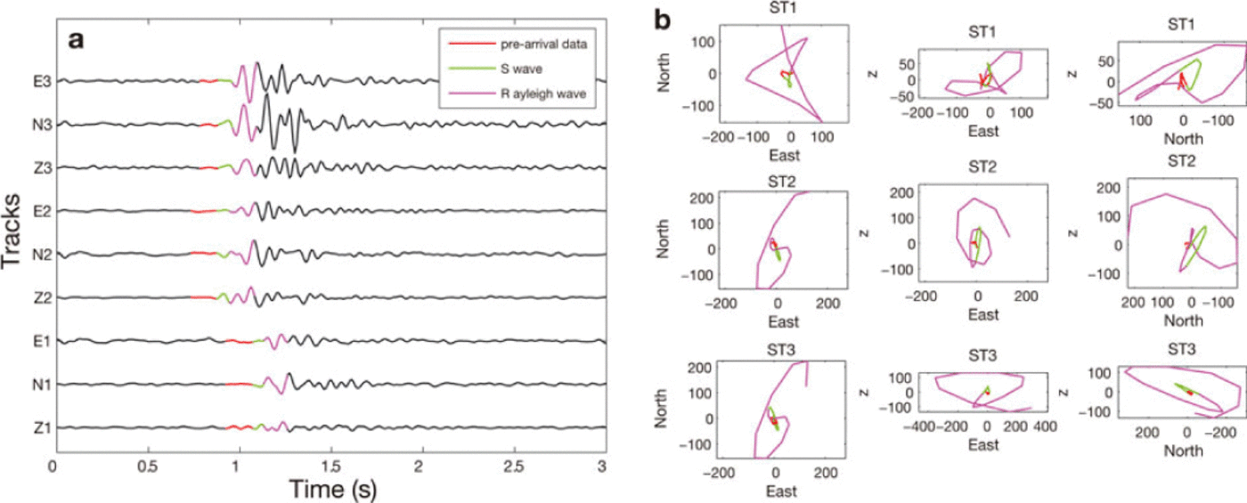
To identify the observed seismic phases, we performed particle motion analysis using the three-component records (Reference Lay and WallaceLay and Wallace, 1995). The three-component seismogram for one event recorded on 5 July on the three seismometers is shown in Figure 4a. Figure 4b shows the associated particle motion in the horizontal and vertical planes, for each sensor. The pre-arrival data, S-wave and Rayleigh wave are depicted by the red, green and magenta portions, respectively. The typical retrograde elliptical motion vertically polarized associated with Rayleigh waves is identified on ST2 and ST3 and to a lesser extent on ST1. The small arrival preceding the Rayleigh wave motion appears to be perpendicularly polarized, in agreement with S-wave polarization. In our experiment, we are presented with small arrival time differences, implying that S-wave coda can overlap with Rayleigh wave arrivals. Consequently, it is difficult to distinguish the two phases. In addition, steep topography implies that Rayleigh waves are not perfectly polarized in the vertical plane.
(a) Three-component event seismograms recorded on ST1, ST2 and ST3 on 5 July (black line), and particle motion in the horizontal (northeast) and vertical (z-east and z-north) planes for each seismometer. The coloured portions in (a) and (b) denote the pre-arrival data (red), the S-wave (green) and the Rayleigh wave phases (magenta).
Location procedure
With the traditional method of locating seismic sources, also known as Geiger’s method (Reference GeigerGeiger, 1910), the hypocentre coordinates (x,y,z) and the origin time, t0
, of an event are determined using a set of arrival times, ![]() , obtained from a microseismic network of k sensors (Reference Lee and StewartLee and Stewart, 1981). For each point, characterized by spatial coordinates (x,y,z) and an origin time t0, theoretical arrival times from the point to the kth sensor are defined by
, obtained from a microseismic network of k sensors (Reference Lee and StewartLee and Stewart, 1981). For each point, characterized by spatial coordinates (x,y,z) and an origin time t0, theoretical arrival times from the point to the kth sensor are defined by ![]() where Tk
is the theoretical travel time derived using a static velocity model (Reference Lee and StewartLee and Stewart, 1981). The method aims at determining the point where the arrival-time residuals (difference between
where Tk
is the theoretical travel time derived using a static velocity model (Reference Lee and StewartLee and Stewart, 1981). The method aims at determining the point where the arrival-time residuals (difference between ![]() and
and ![]() ) are minimized. This optimization problem is generally solved using a least- squares approach, in which the minimum of the sum of the squares of the residuals is retained.
) are minimized. This optimization problem is generally solved using a least- squares approach, in which the minimum of the sum of the squares of the residuals is retained.
The source location was achieved using a grid-search method based on a DEM obtained from Swisstopo aerial photographs taken in 2007. As P- and S-wave arrivals were not distinguishable most of the time, because of the proximity of the seismometers, we used differential arrival times between ST1, ST2 and ST3 in the residuals optimization mentioned above (Reference ZhouZhou, 1994; Reference Font, Kao, Lallemand, Liu and ChiaoFont and others, 2004), in which computation of the origin time, t0 , was not necessary. In this way, the unknowns to be inferred by the inversion process were reduced to source spatial coordinates (x,y,z). Note that the available DEM does not take the ice thickness into account. This implies that sources located in the englaciated zone are assumed to be at the surface and not within the ice mass. It also prevents consideration of the ice/bedrock interface in the ray tracing.
The grid search was applied on the whole DEM, which includes both ice-free and englaciated areas, in order to take into account the potential rockfalls. First results of the procedure were therefore sources distributed in these two zones, and events located in the zone of interest were selected at the end. The different steps of the procedure for one event recorded by our three sensors are:
-
1. For each station, the S-wave phase arrival times (shown in Fig. 4),
 (i = 1,2,3), were picked manually, and differential arrival times, were derived.
 -
2. Each point of the gridded DEM was then considered as a potential source of the detected seismic event. Assuming a static velocity model, we calculated theoretical time lags. We chose 2300ms-1 with reference to the value found by Reference Roux, Marsan, Metaxian, O’Brien and MoreauRoux and others (2008) for the S-wave propagation velocity in granite. This indicates that the part of the ray-path located in the ice could be neglected and thus also the effect of the ice/bedrock interface crossing, which was reasonable for the points in the zone of interest (Reference Roux, Marsan, Metaxian, O’Brien and MoreauRoux and others, 2008). Here we consider that this hypothesis is valid as long as the ice thickness is smaller than the fourth of the dominant period of the recorded seismic signal. As recorded events mostly show a dominant frequency around 20 Hz (see event description below), the fourth of the dominant period ranges around 30 m (using the above-mentioned velocity model), which agrees with our assumption. Moreover, Reference Roux, Marsan, Metaxian, O’Brien and MoreauRoux and others (2008) finally concluded that the relevant velocity parameter was the wave velocity in the rock, as no significant changes in the source locations were observed after modifications in the ice velocity model, which also supports our hypothesis.
-
3. The least-squares minimizations were then performed, by comparing both values
with the error function, ∊:
 were derived.
where σij is the standard deviation of delay measurements for seismometers i and j. This standard deviation must necessarily take into account the uncertainties associated with the time-delay measurements, i.e. in our case, with the picking of the S-wave phase arrivals. The intrinsic error was half of the sampling rate, i.e. 5 ms. Reference Roux, Marsan, Metaxian, O’Brien and MoreauRoux and others (2008) chose this value as standard deviation, but they employed a cross-correlation method for the time delay computation, characterized by a better accuracy than our manual picking. Considering this, we used four half-sampling periods as standard deviation, i.e. 20 ms, for the three seismometers. The retained source was the point of the DEM where ∊ was smallest, i.e. where the observed and theoretical time delays matched best.
Source location verification
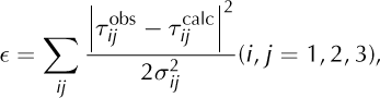
Here we verify the performance of the location procedure using the particle motion analysis (Reference Lay and WallaceLay and Wallace, 1995). The observed ground motion of S- and Rayleigh waves is polarized in the transverse-z and radial planes, respectively. We checked the agreement between location results and particle motion for ten events and present the results for two events with sources located in the zone of interest (red and blue stars in Fig. 5a). For each event, the polarization vector of the Rayleigh wave recorded at each sensor (red and blue arrows in Fig. 5a) was determined with the help of the associated particle motion characteristics (Fig. 5b). We note that in both cases, the orientation of the polarization vectors at each sensor agrees with the polarization of the Rayleigh waves in a longitudinal vertical plane, which qualitatively validates the location of the sources determined using the above location procedure.
(a) Aerial view of the serac fall and polarization vectors of the Rayleigh wave (red and blue arrows) for each sensor, for two events with sources located in the zone of interest (red and blue stars). Empty black squares indicate the sensors. (b) Particle motion characteristics for the two events (upper row for the source at red star, lower row for source at blue star) in the horizontal plane, with signal recorded at each seismometer.
Seismic dataset for the zone of interest
Among the 6320 detected seismic events, 4320 sources were located in the englaciated part of the DEM, with 2426 of them in the zone of interest. The error location range associated with the chosen standard deviation of 20 ms is ±47 m.
Types of events
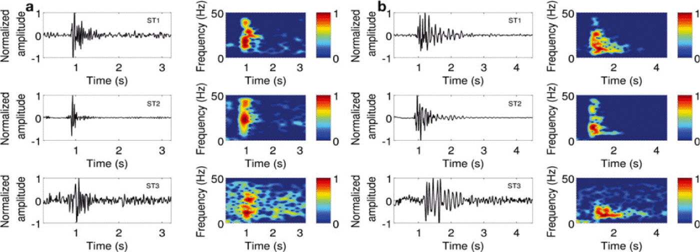
Analysis of the seismic data mainly revealed two different signal types (Figs 6 and 7) characterized by their duration and frequency, similar to the results obtained by Reference Roux, Marsan, Metaxian, O’Brien and MoreauRoux and others (2008). Note that due to our sampling rate, the frequency range was bounded by a Nyquistfrequency of 50 Hz. The first type of event we observed lasts from 0.5 to 2.5 s and exhibits a frequency content ranging between 10 and 30 Hz on at least one station. The signal envelope indicates recurrent patterns, with impulsive onset and smoothly decreasing coda (Fig. 6). The duration and frequency-content characteristics were nevertheless prone to variations (Fig. 6b). We associate them with crack and crevasse openings (Reference Neave and SavageNeave and Savage, 1970; Reference Walter, Deichmann and FunkWalter and others, 2008; Reference Roux, Walter, Riesen, Sugiyama and FunkRoux and others, 2010).
(a, b) Two examples of seismic events, corresponding to a crack opening recorded on the z-component of ST1, ST2 and ST3 and associated normalized spectrograms.
(a) and (b) Two examples of seismic events recorded on the z-component of ST1, ST2 and ST3 and associated normalized spectrograms. The respective durations are 5.5 and 31 s. These events were attributed to icefalls with the help of the location method.
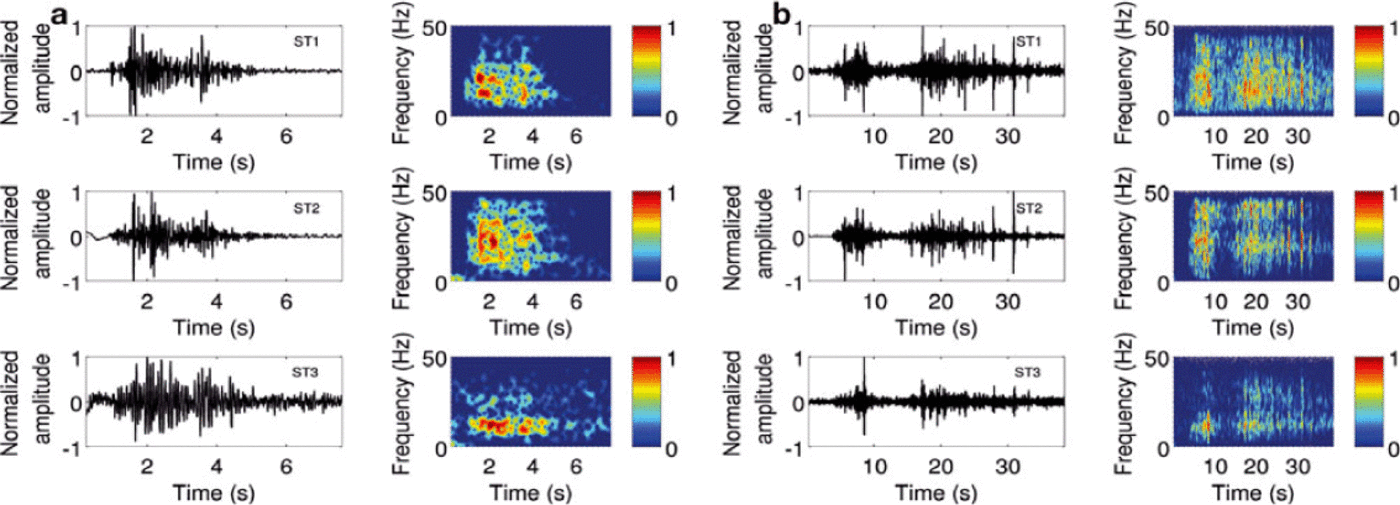
The main characteristic of the second type is the absence of impulsive onset, a duration of several seconds and a complicated spectrum frequency. Figure 7 shows two examples with respective durations of 5.5 and 31 s. The first event exhibits frequencies ranging from 10 to 30 Hz, and the second from 5 to 45 Hz. Both seismograms are characterized by a spindle shape and combine brief impulses dividing the signal.
Whereas the phenomenon leading to the first type of detected events can be identified reliably, the potential cause of the second type has to be analysed carefully. Indeed, rockfalls were likely to occur in the ice-free surrounding zone, and the seismic signal associated with such an event was similar to that triggered by ice-block falls. We thus distinguished between ice- and rockfalls by means of the location, considering that rockfalls do not occur in the englaciated area. Moreover, according to field observations, significant rockfalls likely to be detected on the three sensors were not frequent compared to the occurrences of ice-block falls. We therefore argue that if certain inaccuracies between the two phenomena did occur in our analysis, they did not produce significant changes in our results. Events presented in Figure 7 were located in the englaciated area and thus associated with icefalls. We notice that, contrary to the events triggered by cracks, they are capable of exhibiting several impulses (Fig. 7). We interpret such patterns as potential cracks resulting from the impact of the falling blocks.
Event duration analysis
The duration distribution of the 2426 events located in the zone of interest is shown in Figure 8, with 1 s bins centred from 0.5 to 31.5 s and increment of 1 s. Note that completeness in duration is only reached for values greater than 1 s, which explains the poor amplitude of the leftmost bar. Other work on the microseismicity emitted by glaciers presented crack and crevasse opening as the main source of the detected seismic activity (Reference Roux, Marsan, Metaxian, O’Brien and MoreauRoux and others, 2008; Reference Walter, Deichmann and FunkWalter and others, 2008), the events associated with ice- block falls occurring much less frequently. We see here that 7% of the events have a duration shorter than 1 s, 38% last less than 2 s and more than 8% last more than 12 s. Therefore, the majority of the detected events lasted less than 2 s. The above events analysis showed that this range of duration includes events associated with crack opening, and also with icefalls, which precludes any definite conclusion concerning the predominance of events triggered by crack opening. The only events whose source mechanisms can be unambiguously assessed based on their duration are those shorter than 1 and longer than 12 s. Indeed, the icefalls we analysed never lasted less than 1 s, and we assume that there was no crack formation leading to a seismic event of 12 s duration.
Percentage of detected events with respect to their duration.
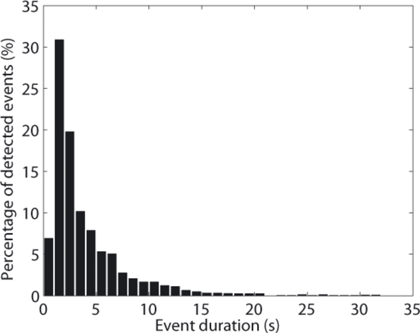
Accordingly, we propose to identify events lasting for less than 1 s with crack opening, and events lasting more than 12 s with the occurrence of icefalls. Events of intermediate duration are likely to be associated with ‘long’ cracks, ‘short’ icefalls or potential glacier slip motion. This point is depicted by the very smooth transition observed between events ranging between 1 and 2 s, and longer events. This indicates that no characteristic event duration can be discerned, and therefore this parameter cannot be used as a criterion for identifying the different event sources in a precise way.
Error assessment
Two Monte Carlo tests were performed in order to estimate the error in location due to the array geometry and the influence of the velocity model (e.g. Reference Roux, Marsan, Metaxian, O’Brien and MoreauRoux and others, 2008). We quantified the effect of array geometry by relocating sources using synthetic arrival times to which noise has been added, and the influence of the velocity model was determined by performing the inversion using different velocity values. We analysed the results for the DEM points in the zone of interest.
In the first test, random errors chosen from a Gaussian distribution with a standard deviation of 20 ms were applied to the three ![]() obtained for each DEM point, in order to simulate errors in
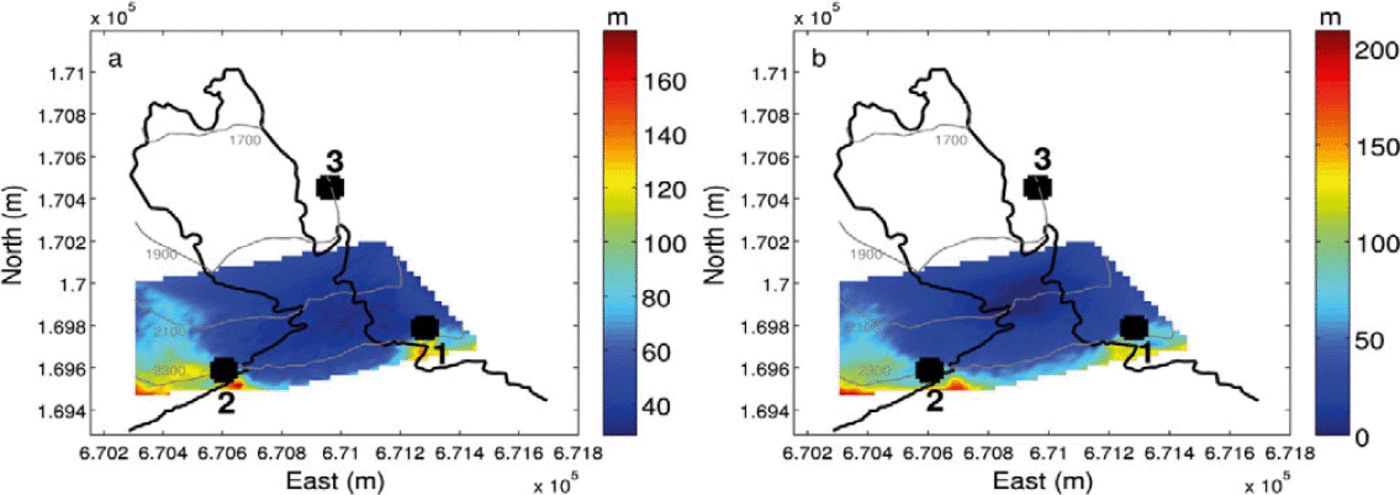
obtained for each DEM point, in order to simulate errors in ![]() . The error range (20 ms) was chosen in agreement with the standard deviation mentioned above, in the location procedure. The grid-search method was then performed and a theoretical source obtained. The procedure was repeated 100 times. An uncertainty was then assigned to every point, by taking the average of the distances between the point and the 100 theoretical sources identified (Fig. 9a). The mean error ranges from 23 to 178 m (Table 1). This error is greater for points outside the array and increases towards the glacier edges in the east-west direction. Errors greater than 100 m are found west of ST2 and east of ST1, with extremes in excess of 150 m at points upstream of the steep part.
. The error range (20 ms) was chosen in agreement with the standard deviation mentioned above, in the location procedure. The grid-search method was then performed and a theoretical source obtained. The procedure was repeated 100 times. An uncertainty was then assigned to every point, by taking the average of the distances between the point and the 100 theoretical sources identified (Fig. 9a). The mean error ranges from 23 to 178 m (Table 1). This error is greater for points outside the array and increases towards the glacier edges in the east-west direction. Errors greater than 100 m are found west of ST2 and east of ST1, with extremes in excess of 150 m at points upstream of the steep part.
Spatial distribution of the mean location error due to (a) array geometry and (b) velocity model, for DEM points distributed between 2050 and 2350ma.s.l. The thick black line marks the englaciated area. The grey elevation lines are at increments of 200m.
Error range in the event location due to the effects of the array geometry and the velocity model
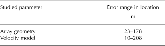
In the second test, we considered each point of the DEM and computed the set of theoretical time delays with a randomly perturbed velocity model. The random perturbation, chosen from a Gaussian distribution, was centred on 2300ms-1 and we set a standard deviation of 500 ms-1. The best model fit was selected as the mean velocity model (2300ms-1), termed ‘reference model’. For a given point, the inversion was performed 100 times by varying the velocity model according to the above standard deviation. For each run, the obtained Tij calc were compared to the Tij computed with the reference model, using the error function referred to above, and we retained the mean of the distances between the point and the 100 sources identified. Results are presented in Figure 9b. The mean error ranges from 10 to 208 m (Table 1). It exhibits a similar spatial distribution to the array geometry error, with slight discrepancies concerning the locations of the extreme values, which also appear in the vicinity of ST2.
In both cases, we observe that the points within the zone of interest are subject to an error less than 50 m. Regarding the above-mentioned error location of 47 m and the mesh grid spacing of 25 m, we consider that a given source location found in the area of interest is reliable to within 50 m.
Spatial distribution of seismic energy emission
Seismic activity can be characterized by two parameters, the number of detected seismic events and the seismic energy release. Reference Deichmann, Ansorge, Scherbaum, Aschwanden, Bernardi and GudmundssonDeichmann and others (2000) and Reference Walter, Deichmann and FunkWalter and others (2008) performed a cluster analysis, whereas Reference Faillettaz, Funk and SornetteFaillettaz and others (2011) employed the energy released by each event to show that their variation obeyed statistical laws. Energy seems to be more appropriate for describing seismic activity because its calculation takes into account signal duration and amplitude, rather than the number of detected events.
Amplitude attenuation
Calculating seismic energy emission is contingent upon correct parameterization of the attenuation of the seismic waves. Indeed, our dataset shows that, depending on the distance between the source and a given seismometer, the recorded amplitudes for one event may exhibit discrepancies, which induces bias in the released energy values and consequently in the use of the associated spatial and temporal distributions. To remedy this, we corrected the recorded seismic amplitudes using (Reference PasoliniPasolini, 2008)
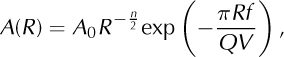
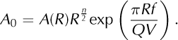
where R is the distance between the source and the seismometer, A(R) is the recorded amplitude, A0 is the amplitude for R = 0, n =1 for surface waves and n = 2 for body waves, Q is a quality factor depending on the medium of propagation, f is a chosen frequency and V is the employed velocity model. The term R-n/1 accounts for the geometrical spreading and the exponential term for the effects of anelastic attenuation. From Eqn (3) we then compute A0 for all detected events:
We set V to 2300 ms-1 and Q to 100 in reference to the attenuation value in granite (Reference IlyasIlyas, 2010). We set f to 25 Hz, choosing this frequency range because it was the most attenuated in spectrograms where discrepancies appeared. R is the distance between the detected source and ST2. The n value was configured to 1, because, as seen in the particle motion study, surface waves constitute the dominant wave phase.
Released energy computation
Using these corrected amplitude values, the energy, E, associated with each detected seismic event was computed using (Reference Amitrano, Grasso and SenfauteAmitrano and others, 2005)
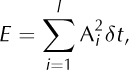
where Ai is the corrected signal amplitude, l is the number of samples and St is the sampling rate. This procedure consisted of manually picking the beginning and end of the event, and numerically integrating the signal recorded at ST2.
The spatial distribution of the released seismic energy was achieved in the following way: considering the whole 74 day dataset, we selected all the seismic events whose source was located at a similar point and summed the associated amounts of released seismic energy. Obtained values were gridded using a nearest-neighbour interpolation, in order to have a better outline of potential clusters. The grid size was 50 m, in agreement with the above location error.
One peculiarity of the zone of interest is that cracks, icefalls and glacier slip motions were likely to occur anywhere within it, as often on the edges as in the central part of the glacier. This means that the location did not allow precise distinction to be drawn between the different types of event. Note that some points of the bedrock were taken into account on the left bank of the glacier since this location was affected by significant icefalls, and consequently by ice blocks rolling on the rock. Moreover, we chose not to take into account the three most energetic events, as they exhibit values more than ten times greater than the others.
The spatial distribution of the released energy is presented in Figure 10a. It exhibits clusters corresponding to points characterized by total released energy of >1 × 10⁹ arbitrary units. We selected five of them, found at various locations and characterized by amounts of released energy ranging from 1.5 × 10⁹ to 2.5 × 10⁹ arbitrary units. The highest energy cluster, ‘a’, is located on the edge of the glacier, the second, ‘b’, is found in the middle of the glacier and the three with the least energy are distributed over the whole area. In order to compare visual observations to such cluster organization and therefore to assess the relevance of the location method, both of them are shown in an aerial plane view of the zone of interest (Fig. 10b). The main finding is that the location of cluster ‘a’ is in agreement with the zone where most of the icefalls were visually observed. This observation is reinforced by the positions of clusters ‘c’ and ‘d’, also found in particularly active areas at the glacier edge. The locations of clusters ‘b’ and ‘e’ are more complicated to interpret because the potential seismicity at these locations was difficult to assess visually. They convey only the enhanced seismic activity in the areas concerned.
(a) Spatial distribution of the released seismic energy (arbitrary units) during the whole study period. Observed clusters are labeled a–e. The thick black line marks the englaciated area. (b) Plot of the clusters (red crosses and letters) on a zoomed view of the zone of interest. The green points denote the sources of the three events not taken into account in the spatial distribution. The altitude contours (black) are spaced 100m apart.
Influence of path effect on signal characteristics
For one given event, we frequently observed discrepancies between the frequency content obtained from data recorded at ST1, ST2 or ST3. In many cases, we noticed that the released energy associated with high frequency (>20 Hz) in spectrograms obtained from the signals recorded at ST1 and ST2 is absent, or much reduced in the spectrogram obtained with ST3 (see Figs 6 and 7). These discrepancies reveal the attenuations affecting the seismic signal recorded at this station, as illustrated by the almost sinusoidal envelope observed for ST3 in Figure 6b. They also indicate that no frequency criterion can be used to precisely distinguish between the different types of event. We notice that the site of the zone of interest implies that most of its points are located closer to ST 1 or ST2 than to ST3. Moreover, the main cluster shown in Figure 10a is significantly closer to ST2 and, besides, is located on the left bank of the glacier. This means, first, that seismic waves detected at ST3 propagated along a longer path than those detected atST1 and ST2 and, second, that they necessarily crossed the glacier. In this regard, we suggest the attenuation of the seismic signals may be due to both the length of the ray-path and the transition between the different mediums crossed. This issue addresses the more general question concerning the lack of information when recording icequakes with sensors installed in the surrounding ice-free area. A first check would be to compare the seismic signal of events recorded simultaneously by sensors installed on the bedrock as well as on or within the ice.
Influence of the trigger on temporal seismic distribution
Water flow at the surface or within the glacier can significantly increase the background noise and therefore induce a considerable trigger bias, as the STA/LTA method is based on signal-to-noise ratio measurements (Reference Walter, Deichmann and FunkWalter and others, 2008). The signal strength of the smallest detectable seismic event consequently depends on the background noise level, and therefore, at least partly, on englacial and supraglacial flow. This is illustrated by a higher sensitivity of the STA/LTA method during time periods of low melt runoff, during which weaker signals are more easily detected (double arrows in Fig. 11a and b). This bias can be due, for instance, to the influence of the diurnal melt cycle, which is likely to induce an artificial diurnal pattern in the temporal seismic activity. Such patterns were identified by Reference Walter, Deichmann and FunkWalter and others (2008), where the authors consequently retained events with amplitude higher than a chosen threshold. In this way, variations in trigger sensitivity were taken into account and the observed temporal changes in the seismic detection represent temporal changes in source activity.
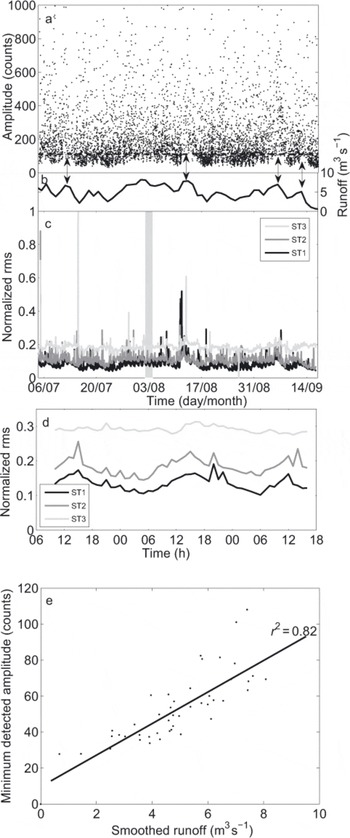
(a) Seismic events (black dots) detected on Triftgletscher from 5 July to 16 September. For the purpose of illustration, only events with amplitudes lower than 1000 counts are shown. The dashed horizontal black line represents the amplitude threshold of 110 counts from which the event detection appears to be independent of the background noise. (b) Smoothed modeled runoff at the icefall, calculated using a 30 hour sliding window. (c) Normalized rms noise for ST1 (black curve), ST2 (dark-grey curve) and ST3 (light-grey curve). (d) Details of the shaded area in (c), between 2 and 4 August. The rms noise was calculated using a 1 hour time window. (e) Minimum detected amplitude according to the smoothed runoff for each sliding window. The thick black line indicates a linear interpolation with a correlation coefficient r 2 = 0.82.
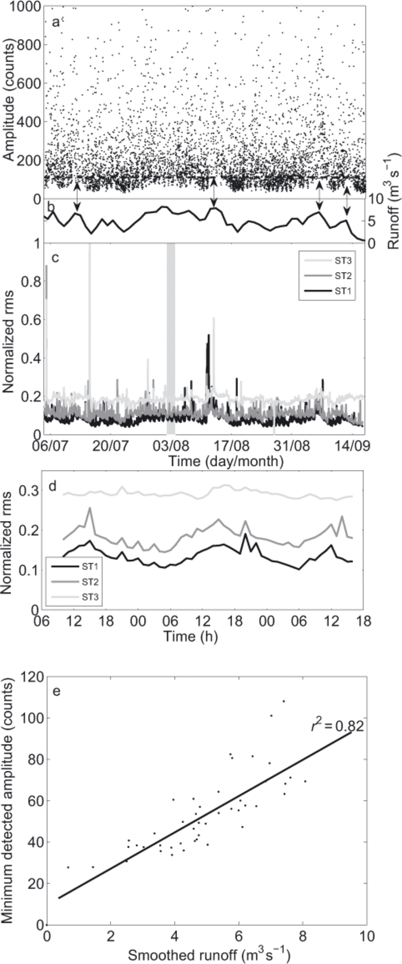
In order to assess the trigger sensitivity variations on Triftgletscher, we analysed the detected seismic events following the method used by Reference Walter, Deichmann and FunkWalter and others (2008) on Gornergletscher. The signal strength of each event was represented by the median of the maximum amplitudes of all seismometers. We used the non-corrected amplitudes and considered all of the 6320 detected events (Fig. 11a).
The results suggest that the main source of change in the trigger sensitivity was not due to diurnal but rather to long-term variations in runoff. We smoothed the modelled runoff values using a sliding window of 30 hours. A simple temporal comparison between smoothed runoff values and minimum detected amplitudes shows that both parameters vary similarly, with increasing smoothed runoff associated with the rise in the minimum detected amplitudes (Fig. 11a and b). Such a relation can be observed in particular on 12 July, 13 August and 6 and 12 September (double arrows in Fig. 11b). In order to determine an amplitude threshold allowing the runoff influence to be eliminated, we performed a more precise analysis by comparing the minimum of the detected amplitudes and the associated mean smoothed runoff value for each sliding window (Fig. 11e). The dependency between the two parameters is shown by the correlation coefficient of 0.82, indicating that changes in the trigger sensitivity are at least partly caused by runoff variations. As the considered amplitudes do not exceed 110 counts, this value appears to be a satisfactory threshold. We also notice that residuals of the linear interpolation tend to increase for large runoff values (Fig. 11e). This can be illustrated, for instance, by the small amplitudes detected around 2 August (Fig. 11b), when runoff was close to the maximum observed value. In this case, the influence of runoff activity on trigger sensitivity was reduced.
In order to more accurately define the impact of background noise on the seismic signal, we analysed the signal strength by calculating the rms, which expressed both the seismic activity and the background noise, for successive temporal windows of 1 hour (Reference Amitrano, Gaffet, Malet and MaquaireAmitrano and others, 2007):
where n is the number of points included in the time window, A is the signal amplitude and St is the sampling period. The calculations were made on the vertical and the horizontal components, but the results showed no significant difference between the two. Figure 11c shows the results for ST1, ST2 and ST3 using the vertical components. We first notice that the highest seismic noise was recorded by ST3, whereas ST 1 and ST2 exhibit similar values. One explanation is the presence of several streams close to ST3, and also the proximity of moraines, where numerous local rockfalls occurred. Three peaks are distinguished, on 5 and 15 July and 11 August. The first two were triggered by teleseisms, and the third was associated with changes in runoff. No rms peak is observed around 2 August, confirming the above- mentioned limited role played by runoff in ambient noise at this time.
The sub-daily analysis during a 2 day time period (shaded area in Fig. 11 c) indicates clear diurnal patterns for ST 1 and ST2, with minimum rms noise at 04:00 and maximum at 1 6:00. The seismic signal, at least for these two stations, also appears to be affected by the diurnal melt cycle. One reason for the absence of significant diurnal influence in the signal coming from ST3 may be that the streams flowing close to the sensor are not connected to the glacier, decreasing the dependence of the signal on the time of day. Except for the water drainage diurnal pattern, the rms noise does not show a spatial pattern, either at a daily or a sub-daily timescale.
After applying the threshold value of 110 counts to the 2426 events located in the zone of interest, in the following we consider only the 1792 events remaining.
Discussion
Our analysis yields the following results: First, it is possible to monitor the acoustic emissions originating from the glacier with seismometers not directly installed on the ice. Second, the local microseismic activity on Triftgletscher is due mostly to crack openings and icefalls; however these two sources cannot be distinguished precisely by means of the duration or the frequency content. Third, the released seismic energy appears to be spatially organized and cluster locations support visual observation. Moreover, consideration of the influence of the trigger appears to be crucial to the assessment of the temporal evolution of seismic activity.
Using a statistical approach, Reference Faillettaz, Funk and SornetteFaillettaz and others (2011) showed thatfor mechanical instabilities an increasing surface motion prior to the break-off in 2005 on Weisshorngletscher was correlated with rising seismic activity, and defined this rise as a relevant precursor of potential break-off. Here we investigate the potential relationship between runoff, surface motion and released seismic energy with the help of such a statistical law, and assess whether seismic precursors for break-off events can be determined in the case of sliding instability.
Runoff data and basal water pressure
Using ice thicknesses and slopes measured in the central part of Unteraargletscher, Switzerland, Reference IkenIken (1981) studied the relationship between enhanced glacier motion and the growing size of basal water pockets due to increasing water pressure, by means of an idealized numerical model. The sliding phenomena observed at Balmhorngletscher and Allalingletscher, Switzerland (Reference ROthlisberger and KasserRothlisberger and Kasser, 1978; Reference Rothlisberger, Kasser and HaeberliRothlisberger, 1981b, Reference Rothlisberger1987), were also explained by this process. Reference Walter, Deichmann and FunkWalter and others (2008) observed significantly higher basal seismic activity during periods with decreasing subglacial water pressure. Subglacial water-pressure changes play a crucial role in glacier dynamics and are consequently connected to its seismic response. In our case, only daily runoff and modelled hourly runoff data are available and a key question is their reliability for inferring the subglacial water-pressure variations. Reference AndersonAnderson and others (2004) and Reference Bartholomaus, Anderson and AndersonBartholomaus and others (2008) observed a strong feedback between subglacial hydrology and sliding for Bench and Kennicott Glaciers, Alaska. In both studies melt runoff and precipitation were used, indicating that melt runoff can reasonably be identified with basal runoff and may be linked to subglacial water pressures. In light of these results, we assume in the following that runoff changes are associated with basal water-pressure variations.
Comparison between runoff and surface motion
In order to assess the influence of the runoff on the surface motion at a timescale of several days, we compared for each of the time intervals, Δ ti,ti +24h, the mean surface motion and the associated mean modelled runoff values. As we aimed to focus on the zone of interest, we determined surface motion from points located on a flowline (black line in Fig. 3) chosen in the middle of this area. For each interval, the retained runoff was the mean of the modelled values.
Results are presented for two study periods running from 26 July to 7 August (Fig. 12a) and from 26 August to 6 September (Fig. 12b). Runoff values were smoothed with a 24 hour overlapping sliding window. Indicated times correspond to the middle of each temporal interval (black crosses in Fig. 2). The temporal evolution of the correlation coefficient, r2, between the two parameters using sliding windows of ten values is shown by the bars at the bottom of the figures; r2 = 1 indicates a perfect correlation while r2 = —1 means that the parameters are anticorrelated. The runoff error (vertical lines) allows us to consider runoff changes at a timescale of several days only, because of the low amplitudes observed in the variation from one 24 hour period to the next.
Smoothed mean modelled runoff (blue curve) and surface motion (red curve) for time periods (a) 26 July to 7 August and (b) 26 August to 6 September. For each runoff and surface motion, one given value is computed for each of the time intervals, Δ ti,ti +24h, indicated in Figure 2. Mean surface motion is computed using points distributed on the flowline indicated in Figure 3. Bars show the evolution of the correlation coefficient. Data were obtained with sliding windows of ten values of both parameters. Observed peaks of motion are labeled P1–P6. Blue vertical lines denote runoff error.
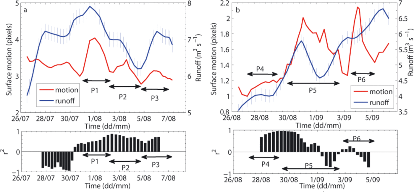
The first study period (26 July to 7 August; Fig. 12a) exhibits mean runoff values from 5.4 to 7.5 m3 s-1 and surface displacements ranging from 2.7 to 4.1 pixelsd-1. The surface motion shows three main peaks, P1, P2 and P3. In the time period P1-P3, changes in surface motion are satisfactorily explained by runoff variations (r2 > 0.4). The smallest values may be due to punctual time shifts between the two parameters. Before P1, r2 are negative, the parameters being anticorrelated. We propose to interpret the strong increasing runoff, coupled with a slightly decreasing motion, as a water storage process caused by an inefficient drainage system. This storage may be coupled to an increasing basal water pressure likely to lead to P1 when a pressure threshold is exceeded.
The second period (26 August to 6 September; Fig. 12b) exhibits mean runoff values between 3.5 and 6.5 m3 s-1 and surface displacements ranging from 1.0 to 2.1 pixels d-1. We notice that both the studied parameters evolve in lower ranges than during the first study period and that both exhibit a positive trend. Three peaks of motion, P4, P5 and P6, are observed. Runoff changes satisfactorily explain surface motion until the middle of P5 (r2 > 0.4). After P5, r2 values are negative or ~0, but both parameters still exhibit a common positive trend. This indicates that the influence of the runoff on the surface motion decreased at this time, butthat the positive correlation at a timescale of several days is still verified.
This analysis brings to light several results. First, good agreement between changes in runoff and surface motion is supported by r 2 > 0.4, or at least by a similar trend for both parameters. Second, potential inefficiency of the basal water drainage system can explain the observed discrepancies. Third, the comparison between the two periods of survey (late July and late August) shows that a higher range of runoff was associated with a higher range of surface motion. Regarding these findings, we consider that changes in motion at a timescale of 2-3 days can reasonably be approached by means of the modelled runoff variations.
Seismic sources differentiation with a statistical analysis
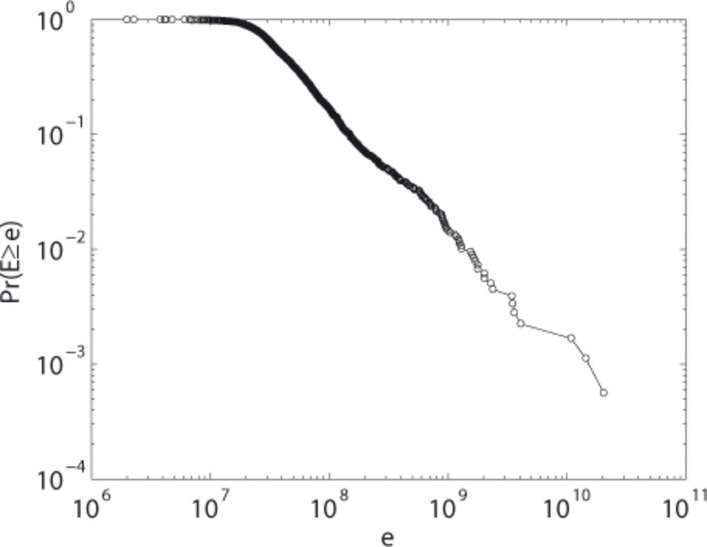
We previously saw that neither the frequency content nor the event duration allows the different seismic sources to be distinguished precisely. Here we investigate whether the latter could be differentiated by means of a statistical analysis of the released seismic energy. Our study is based on the method of Reference Faillettaz, Funk and SornetteFaillettaz and others (2011). In order to assess the size/frequency distribution of the detected icequake energy for the whole dataset, we first determined its complementary cumulative size/frequency distribution (CSFD) (Fig. 13). The CSFD indicates the probability Pr(X ≥ x) that a variable, X, takes a value greater than a given value, x (Reference Faillettaz, Funk and SornetteFaillettaz and others, 2011). In our case, it denotes the probability that the energy, E, released by an icequake will exceed a given value, e (Pr(E ≥ e)). For dependent occurrences, the CSFD is well fitted by an exponential function, p ~ a exp(bx). By contrast, a CSFD generated by independent events is fitted by a power law, p ~ x-β (Reference Faillettaz, Funk and SornetteFaillettaz and others, 2011). As no break-off was observed during the study period, we assume the detected events are independent. A power law is characterized by a given exponent, β estimated using the maximum-likelihood fitting method with goodness-of-fit based on the Smirnov test (Reference Clauset, Shalizi and NewmanClauset and others, 2009). For a given time series of icequake released energy, the plausibility of the power law was quantified using the p-value generated by this goodness-of-fit test and we accepted the power- law hypothesis for β values higher than 0.2 (Reference Faillettaz, Funk and SornetteFaillettaz and others, 2011).
Complementary cumulative size/frequency distribution,Pr(E ≥ e), of icequake energy, E (arbitrary units), for the whole dataset.
A change in β expresses modifications in the size/frequency distribution, i.e. in our study, changes in the distribution of the released seismic energy. A high β value conveys a low number of high-energy events compared with low-energy events, and a low β value conveys the opposite. In the following, high-energy events are called ‘big events’ and low-energy events ‘small events’.
The size/frequency distribution shown in Figure 13 is characterized by a p-value of 0, rejecting the power-law hypothesis. This result can be explained by the excess of events found at ~109 arbitrary units preventing any power- law fitting. Here again, the different sources of energy are mixed up with each other and no distinction is possible.
For a more accurate analysis, we scrutinized the temporal variation of the CSFD, using a moving window of 200 events with a time shift of 10 events. For each window, the distribution of the released seismic energy was assessed and the power-law hypothesis tested. Results are shown in Figure 14. Over the 159 considered time windows, 148 (empty symbols) are characterized by a CSFD generated by a power law. Moreover, the associated β exponent significantly varies with time from ~1 to 1.9, thereby denoting changes in the released seismic energy distribution. Two examples of CSFDs with a p-value higher than 0.2 are depicted at the top of Figure 14. In both cases we see good agreement between the distribution and the power law (dashed black line) with, nevertheless, discrepancies for the most energizing events.
The lower plot shows the evolution of the exponent β of the power law fitting the CSFD, Pr(E ≥ e), obtained in running windows of 200 events with a time shift of 10. Empty symbols indicate fits with a p-value greater than 0.2, i.e. when a power-law behavior is plausible. The horizontal lines refer to the sliding-window size. The vertical lines indicate the goodness-of-fit for each β value. The two plots at the top show details of CSFDs obtained in two of the windows.
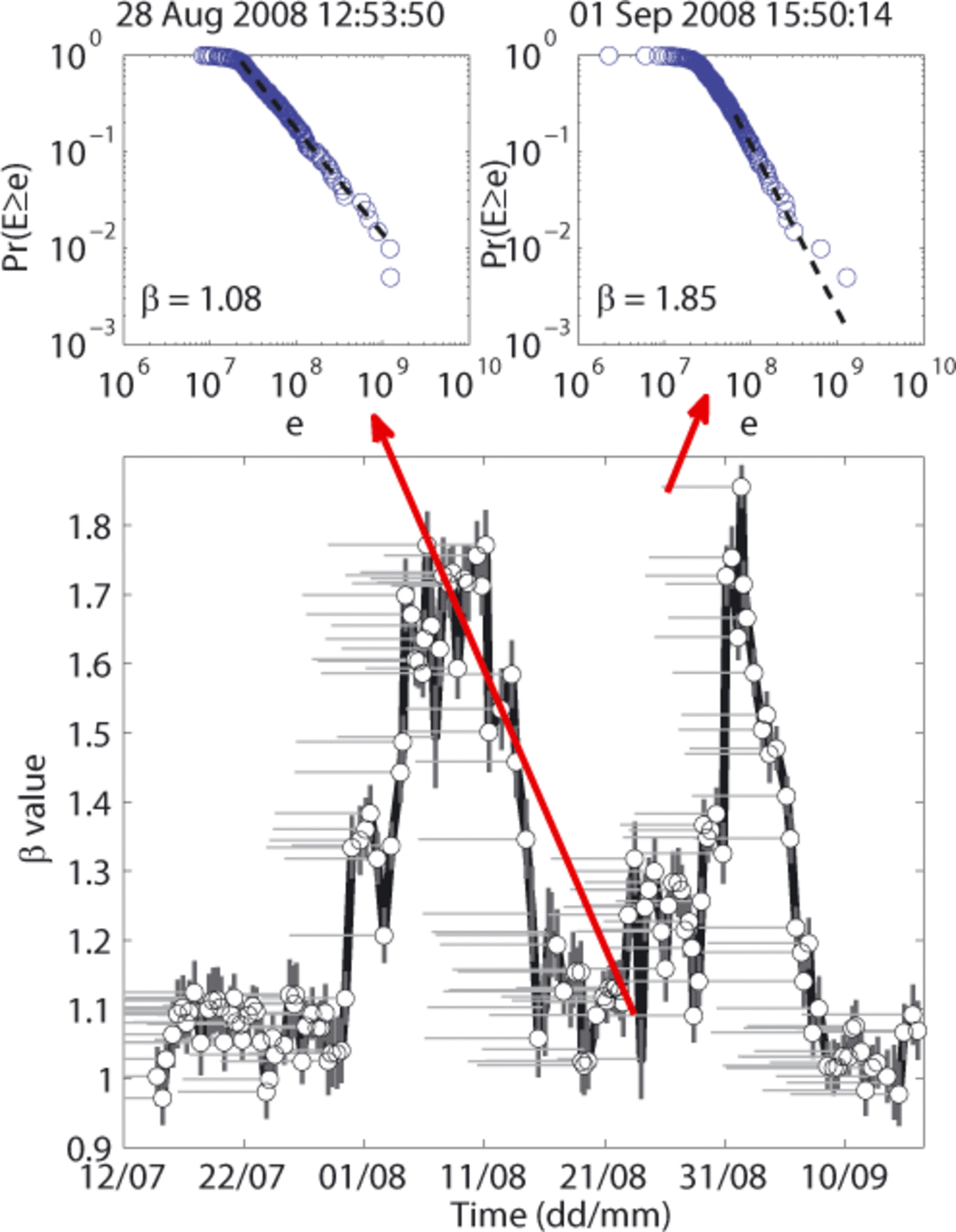
In order to assess the meaning of these β changes, we compared their evolution with the modelled runoff time series (Fig. 15). The analysis was performed using sliding windows of 200 events with a time shift of 10. The runoff value associated with each window was the mean of the runoff modelled during the interval. With regard to observed changes in runoff regime, and therefore in the surface motion with reference to what was shown above, two ranges of β values, r1 and r2, were defined (shaded areas in Fig. 15). The lowest, r1, chosen between 0.95 and 1.15, is associated with the lowest observed runoff values. At these times big events predominated. The second, r2, chosen between 1.4 and 1.9, concerns time intervals when runoff was largest or increasing. At these times the seismic activity was mostly due to small events. The CSFD characterized by intermediate β values refers to transition phases between r1 and r2. During periods of increasing surface motion, β values generally rise, conveying a transition towards small events, whereas during periods of decreasing motion β values generally decrease.
Temporal evolution of β exponent (black curve) and modelled runoffs (blue curve) obtained in running windows of 200 events with a time shift of 10. The circles indicate the windows characterized by a p-value greater than 0.2. The two shaded areas stand for the β value ranges we called r1 and r2. Blue vertical lines denote runoff error.
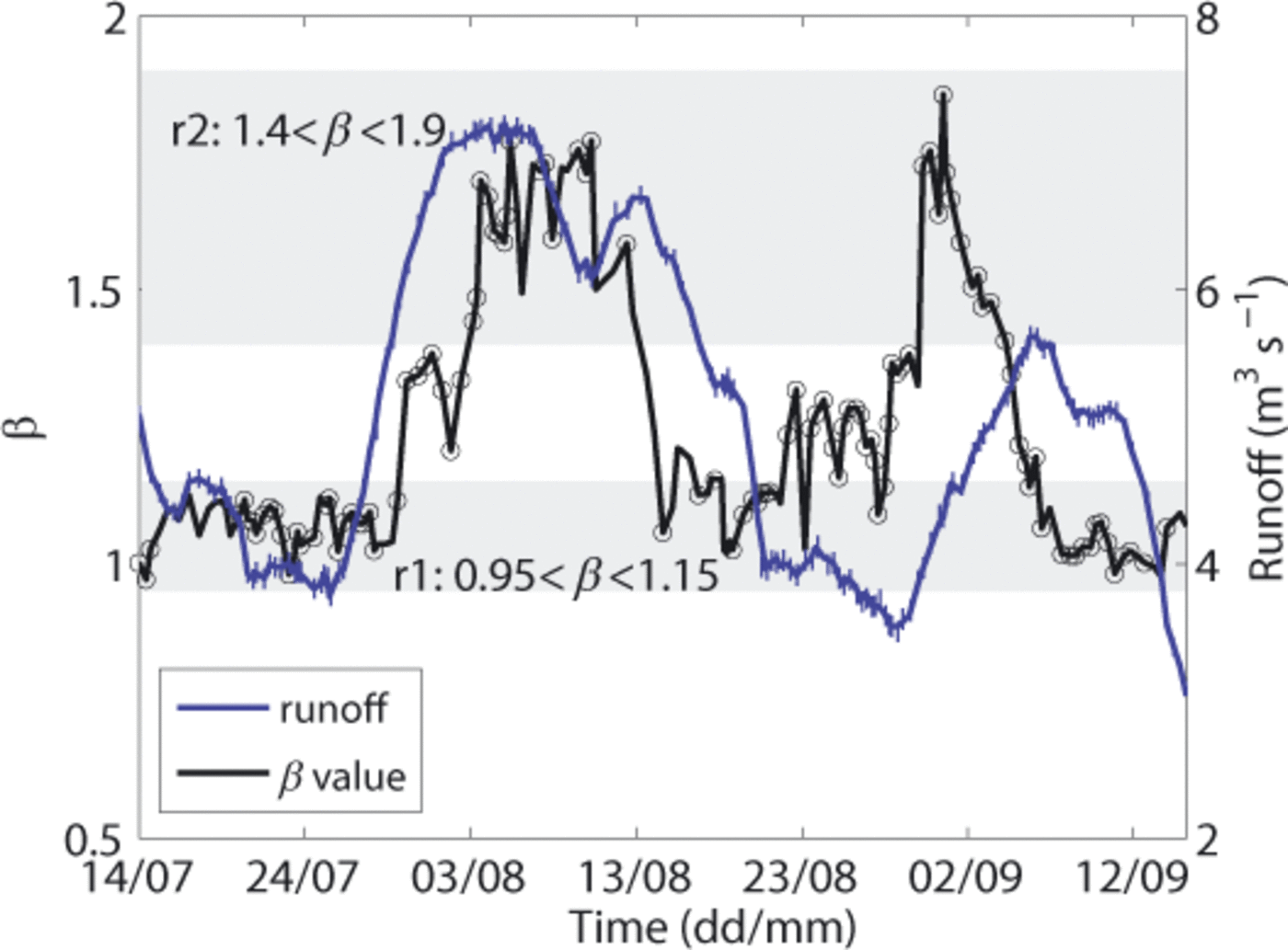
The influence of surface motion (through runoff changes) on the released seismic energy distribution (3 values) is well established from the beginning of the study period until the end of August. The discrepancy existing for the rest of the time might be explained by the poorer agreement between runoff and surface motion during this period (see Fig. 12b).
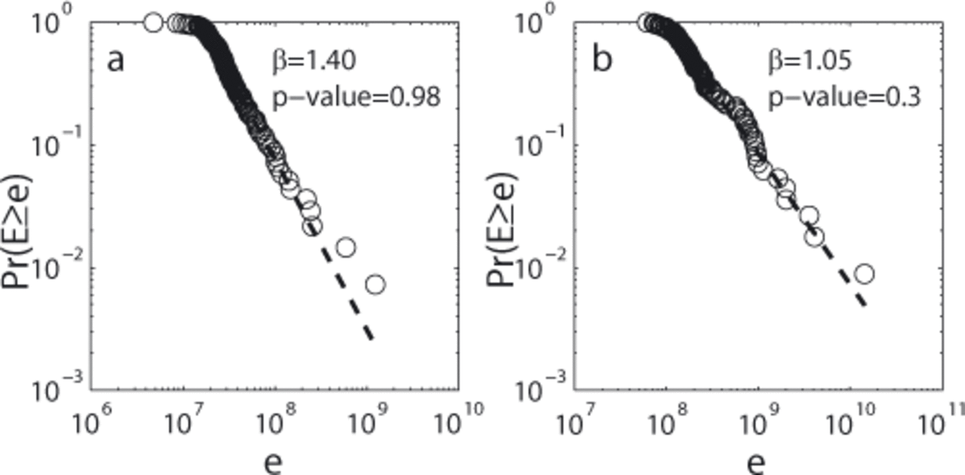
In order to assess what types of event are most likely related to r1 or r2, we examined the CSFDs (Fig. 16) of events unambiguously triggered by cracks (<1 s) as well as of those most likely triggered by icefalls (>12s). We see that both follow a power law. Moreover, we notice that the 3 value of the crack event distribution (Fig. 16a) ranges in r2 while the second one (Fig. 16b) is included in r1. This may indicate that events occurring during rapid surface motion could be triggered by cracks opening, and that low or decreasing surface motion may favour the highest-energy events (e.g. large-extent icefalls). The events characterizing the transition phases may be linked to intermediate events as ‘long’ cracks or ‘low-extent’ icefalls. They may also correspond to glacier slip motion events, but there are no clues that allow us to distinguish them precisely. However these statements are to be treated with caution, given the poor p-value associated with the CSFD of the icefall events.
CSFD, Pr(E ≥ e) for events (a) shorter than 1 s and (b) longer than 12 s.
Seismic precursors for break-off
We saw above that the ,β-value echanges are associated with modifications in the distribution of released seismic energy. However, this analysis was applied to reduced time windows, and a longer investigation timescale of both the released energy and the runoff appeared relevant, especially for detecting potential seismic precursors for break-off.
The temporal evolution of released seismic energy and that of runoff (Fig. 17) exhibit three peaks: E1, E2, E3 and Q1, Q2, Q3, respectively. We assume that only the descending phase of Q1 is visible. By removing the three highest-energy events from the time series (thin dashed black curve in Fig. 17), we notice that both duration and amplitude of the energy peaks were strongly conditioned by the occurrence of these events (green and red circles in Figs 10b and 17, respectively). However, as these events emphasized pre-existing lower-extent peaks, we consider E1, E2 and E3 as being reliable, in spite of the influence of the sliding- window analysis.
Modelled runoff evolution (blue curve) and released seismic energy with (green curve) and without (dashed black curve) the three highest-energy events of the time series (red circles), obtained with sliding windows of 200 events and a time shift of 10. Peaks of released energy and runoff are labelled E1, E2, E3 and Q1, Q2, Q3, respectively. Blue vertical lines denote runoff error.
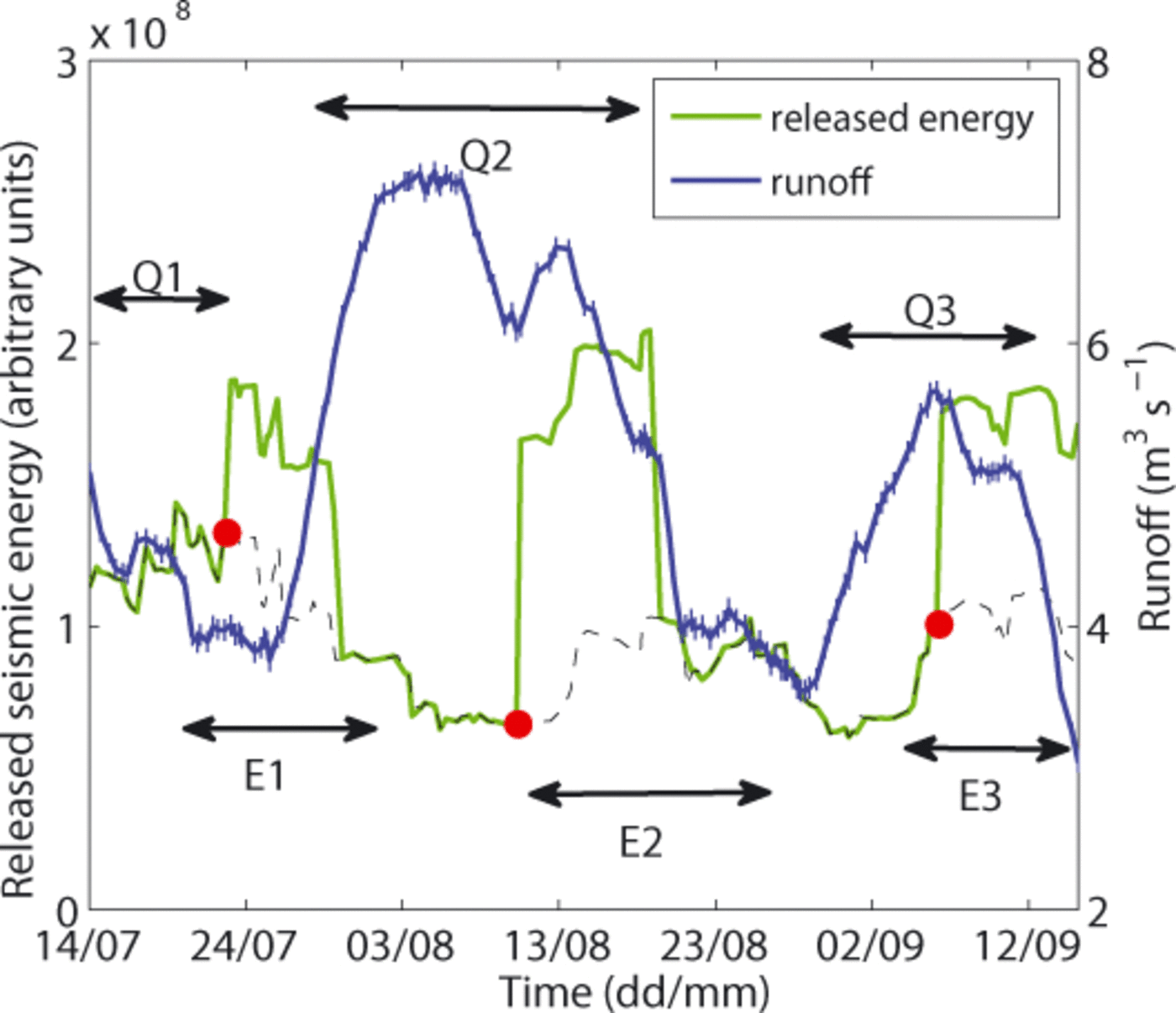
E1, E2 and E3 were similarly coupled with minimum or decreasing runoff, i.e. with low or decreasing basal water pressure and finally with low or decreasing surface motion. Such phases may coincide with glacier recoupling processes, likely to cause the observed energy peaks.
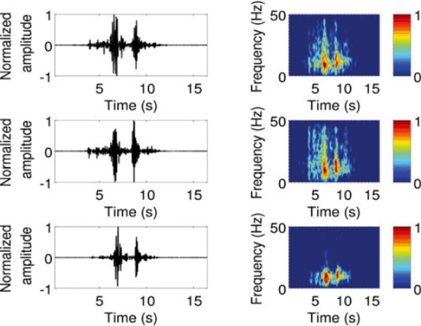
The three highest-energy events show their sources in the top middle part of the serac fall (Fig. 10b) and lasted 8-12 s. The associated seismograms present a similar spindle shape, combined with several consecutive strong impulses, and emit a maximum energy at a frequency around 10 Hz on the three spectrograms (Fig. 18). Moreover, all three were recorded during decreasing runoff. Given these characteristics, we suggest they were most probably not triggered by icefalls, and propose that they are associated with the glacier recoupling. The observed strong impulses may illustrate the jerky motion of the glacier at this time, due to the increased grip of the ice on the bedrock caused by decreasing basal water pressure. On this assumption, we suggest that such an event may have characterized a decreasing glacier slip motion. This is supported, first, by the location of the associated sources, in the steepest part of the zone of interest, and, second, by the duration and frequency (Reference Weaver and MaloneWeaver and Malone, 1979).
High-energy seismic event of 23 July recorded on the northcomponentof ST1, ST2 and ST3 (left) and associated normalizedspectrograms (right).
For sliding instabilities, as in the case of Triftgletscher, Rothlisberger (1981a) showed that break-offs are preceded by surface motion accelerations called ‘active phases’, but he also showed that these phases are not always followed by a break-off. For such an event, he suggested that changes in the subglacial drainage system during the ‘active phase’ induce recoupling of the ice with the bedrock, which in turn stops the enhanced sliding phase. Our findings tend to support this assertion, in the sense that in our study the recouplings accompanying the falls of basal water pressure are illustrated by the observed energy peaks E1, E2 and E3.
However, we propose that the amount of energy released during the recoupling phase may also weaken the glacier by damaging the ice and possibly lead to a break-off. In this way, a potential seismic precursor may be the detection of a peak of released energy similar to E1, E2 or E3, this peak indicating the temporary weakness of the glacier and therefore an enhanced break-off risk. A more precise clue for enhanced break-off risk may also be the detection of seismic eventssimilar to those we associated above with glacier recoupling, as they denote the temporary weakness of the glacier in a more confined time interval. This nevertheless remains uncertain, as we only detected three such events. The influence of the ice recoupling on break-off risk thus appears to change according to the considered timescale. If at a long-term time scale it can point out an aborted break-off event, it may also be interpreted as an enhancing factor during the time when it occurs, due to the potential destabilization it can induce.
The seismic method also brings two main improvements compared to the surface motion criteria: (1) It enables the dynamics of the ice mass as a whole to be monitored continuously, whereas surface motion measurements provide only point measurements. We can therefore expect a more reliable detection of the ‘active phases’ and thus a greater relevancy of the latter with respect to potential break-off prediction. (2) In a more practical way, seismic monitoring is independent of the prevailing meteorological conditions, which is not the case for surface motion monitoring.
Conclusion
A high seismic emissivity was recorded from the steep part of Triftgletscher. Focusing on the englaciated area ranging from 2050 to 2350ma.s.l., 2426 events were detected over the 74day study period. Events associated with crack openings and icefalls were recognized but neither the duration nor the frequency content allowed a precise distinction to be made between the two sources. The event detection sensitivity was influenced significantly by the water flow intensity, which also partly explains the observed background noise. Icequake clusters were depicted in the spatial distribution of the released seismic energy and showed good agreement with visual observations of the seismic activity, supporting the relevance of the location method used. The surface motion affecting the zone of interest appeared to be satisfactorily explained by runoff changes, which allowed us to compare the seismic activity with the glacier dynamics over the entire study period. The distribution of the released seismic energy was investigated by means of a statistical analysis, and two regimes of seismicity were highlighted. Low- and high-energy events were detected predominantly during periods of high and low surface motion, respectively. We characterized glacier recoupling by peaks of released energy and proposed two potential seismic precursors for break-off based on this: a peak of released energy ranging over several days or, more hypothetically, the detection of a very high-energy event likely to indicate glacier recoupling.
As a next step, valuable information is expected to be revealed about the source mechanisms by drawing a more accurate distinction between the various events. The lack of information linked to the crossing of the ice interface could be investigated by comparing signals recorded simultaneously in the ice and on the bedrock. Active seismic experiments should, in theory, enable wave velocity and potential wave paths through the complex medium formed by the glacier and the underlying bedrock to be assessed accurately.
Acknowledgements
This work was supported by the EU-FP7 ‘ACQWA’ Project (www.acqwa.ch) under contract No. 212250. We are indebted to two anonymous reviewers and Alex Brisbourne for helpful comments. We are grateful to many members of the VAW, the Swiss Seismological Service of ETH, C. Senn, who assembled our instruments, and KWO which supplied daily runoff data. The Swiss military provided valuable support by transporting equipment via helicopter. We thank N. Deichmann for constructive comments during the preparation of the manuscript, and Susan Braun-Clarke for proofreading the English.