


1 Introduction
In factor analysis, a potentially large set of dependent random variables is modeled as a linear combination of a smaller set of underlying latent (unobserved) factors. Factor analysis is ubiquitously applied in fields, such as econometrics (Aigner et al., Reference Aigner, Hsiao, Kapteyn and Wansbeek1984; Aßmann et al., Reference Aßmann, Boysen-Hogrefe and Pape2016; Fan et al., Reference Fan, Fan and Lv2008), psychology (Caprara et al., Reference Caprara, Barbaranelli, Borgogni and Perugini1993; Ford et al., Reference Ford, MacCallum and Tait1986; Goretzko et al., Reference Goretzko, Siemund and Sterner2023; Horn, Reference Horn1965; Reise et al., Reference Reise, Waller and Comrey2000), epidemiology (de Oliveira Santos et al., Reference de Oliveira Santos, Gorgulho, de Castro, Fisberg, Marchioni and Baltar2019; Martínez et al., Reference Martínez, Marshall and Sechrest1998), and education (Beavers et al., Reference Beavers, Lounsbury, Richards, Huck, Skolits and Esquivel2013; Schreiber et al., Reference Schreiber, Nora, Stage, Barlow and King2006). It also has applications in causality (Pearl, Reference Pearl2000; Spirtes et al., Reference Spirtes, Glymour and Scheines2000) as a building block for models with latent variables (Barber et al., Reference Barber, Drton, Sturma and Weihs2022; Bollen, Reference Bollen1989).
Let $X=(X_v)_{v \in V}$
be an observed random vector, and let
$X=(X_v)_{v \in V}$
be an observed random vector, and let $Y=(Y_h)_{h \in \mathcal {H}}$
be a latent random vector, indexed by finite sets V and
$Y=(Y_h)_{h \in \mathcal {H}}$
be a latent random vector, indexed by finite sets V and $\mathcal {H}$
, respectively. Factor analysis models postulate that each observed variable
$\mathcal {H}$
, respectively. Factor analysis models postulate that each observed variable $X_v$
is a linear function of the factors
$X_v$
is a linear function of the factors $Y_h$
and noise, that is,
$Y_h$
and noise, that is,
 $$\begin{align*}X = \Lambda Y + \varepsilon, \end{align*}$$
where $\Lambda = (\lambda _{vh}) \in \mathbb {R}^{|V| \times |\mathcal {H}|}$
is an unknown coefficient matrix known as the factor loading matrix. The elements of
$\Lambda = (\lambda _{vh}) \in \mathbb {R}^{|V| \times |\mathcal {H}|}$
is an unknown coefficient matrix known as the factor loading matrix. The elements of $\varepsilon = (\varepsilon _v)_{v \in V}$
are mutually independent noise variables with mean zero and finite, positive variance. We consider orthogonal factor analysis, which means that we assume that the latent factors
$\varepsilon = (\varepsilon _v)_{v \in V}$
are mutually independent noise variables with mean zero and finite, positive variance. We consider orthogonal factor analysis, which means that we assume that the latent factors $(Y_h)_{h \in \mathcal {H}}$
are mutually independent. The model further assumes that
$(Y_h)_{h \in \mathcal {H}}$
are mutually independent. The model further assumes that $\varepsilon $
is independent of Y. Without loss of generality, we fix the scale of the factors such that
$\varepsilon $
is independent of Y. Without loss of generality, we fix the scale of the factors such that $\text {Var}[Y_h]=1$
for each factor. The main object of study, the covariance matrix of the observed random vector X, is then given by
$\text {Var}[Y_h]=1$
for each factor. The main object of study, the covariance matrix of the observed random vector X, is then given by
 $$ \begin{align} \Sigma := \text{Cov}[X] = \Lambda \Lambda^{\top} + \Omega, \end{align} $$
where $\Omega $
is a diagonal matrix with entries
$\Omega $
is a diagonal matrix with entries $\omega _{vv}= \text {Var}[\varepsilon _v]$
.
$\omega _{vv}= \text {Var}[\varepsilon _v]$
.
Our focus is on confirmatory factor analysis (Bollen, Reference Bollen1989, Chapter 7), which pertains to a prespecified model that encodes a scientific hypothesis or was learned previously in an exploratory step. Most interest is typically in models in which the factor loading matrix $\Lambda $
is sparse. In this article, we assume that the sparsity structure of the factor loading matrix and the number of latent factors
$\Lambda $
is sparse. In this article, we assume that the sparsity structure of the factor loading matrix and the number of latent factors $|\mathcal {H}|$
are fixed and known. Estimation of the factor loadings in confirmatory analyses has been subject to much controversy, due to the difficulties in determining model identifiability (Long, Reference Long1983). A factor analysis model is identifiable if the loading matrix
$|\mathcal {H}|$
are fixed and known. Estimation of the factor loadings in confirmatory analyses has been subject to much controversy, due to the difficulties in determining model identifiability (Long, Reference Long1983). A factor analysis model is identifiable if the loading matrix $\Lambda $
can be recovered from the covariance matrix
$\Lambda $
can be recovered from the covariance matrix $\Sigma $
in (1). If
$\Sigma $
in (1). If $\Lambda $
is not identifiable, then its estimates are to some degree arbitrary and standard inferential methods invalid (Cox, Reference Cox2024; Ximénez, Reference Ximénez2006).
$\Lambda $
is not identifiable, then its estimates are to some degree arbitrary and standard inferential methods invalid (Cox, Reference Cox2024; Ximénez, Reference Ximénez2006).
In full factor analysis, where no restrictions on the factor loading matrix are imposed (Drton et al., Reference Drton, Sturmfels and Sullivant2007), the matrix $\Lambda $
is never identifiable, due to rotational invariance. Indeed, for any orthogonal matrix
$\Lambda $
is never identifiable, due to rotational invariance. Indeed, for any orthogonal matrix $Q \in \mathbb {R}^{|\mathcal {H}| \times |\mathcal {H}|}$
, the product
$Q \in \mathbb {R}^{|\mathcal {H}| \times |\mathcal {H}|}$
, the product $\widetilde {\Lambda } = \Lambda Q$
satisfies
$\widetilde {\Lambda } = \Lambda Q$
satisfies
 $$\begin{align*}\widetilde{\Lambda} \widetilde{\Lambda}^{\top} + \Omega = \Lambda Q Q^{\top} \Lambda^{\top} + \Omega = \Lambda \Lambda^{\top} + \Omega \end{align*}$$
and, thus, $(\widetilde {\Lambda },\Omega )$
determines the same covariance matrix as
$(\widetilde {\Lambda },\Omega )$
determines the same covariance matrix as $(\Lambda ,\Omega )$
. For this reason, prior work on full factor analysis focuses on identifiability of
$(\Lambda ,\Omega )$
. For this reason, prior work on full factor analysis focuses on identifiability of $\Lambda \Lambda ^{\top }$
or, equivalently, of
$\Lambda \Lambda ^{\top }$
or, equivalently, of $\Omega $
. Bekker and ten Berge (Reference Bekker and ten Berge1997) characterize generic identifiability, which refers to whether
$\Omega $
. Bekker and ten Berge (Reference Bekker and ten Berge1997) characterize generic identifiability, which refers to whether $\Omega $
can be uniquely recovered for almost all parameter choices, except for a few corner cases at the so-called Ledermann bound. However, for models with sparsity restrictions on
$\Omega $
can be uniquely recovered for almost all parameter choices, except for a few corner cases at the so-called Ledermann bound. However, for models with sparsity restrictions on $\Lambda $
, the situation may improve, allowing for the identifiability of the loading matrix
$\Lambda $
, the situation may improve, allowing for the identifiability of the loading matrix $\Lambda $
itself up to sign changes of the columns. Identifiability up to column sign is the best we may hope for. If we multiply
$\Lambda $
itself up to sign changes of the columns. Identifiability up to column sign is the best we may hope for. If we multiply $\Lambda $
with a diagonal matrix
$\Lambda $
with a diagonal matrix $\Psi $
with entries in
$\Psi $
with entries in $\{\pm 1\}$
, then the support of
$\{\pm 1\}$
, then the support of $\Lambda \Psi $
is the same as the support of
$\Lambda \Psi $
is the same as the support of $\Lambda $
and it still holds that
$\Lambda $
and it still holds that $\Lambda \Psi \Psi ^{\top } \Lambda ^{\top } = \Lambda \Lambda ^{\top }$
.
$\Lambda \Psi \Psi ^{\top } \Lambda ^{\top } = \Lambda \Lambda ^{\top }$
.
Example 1.1. In a re-analysis of a well-known five-dimensional example of Harman (Reference Harman1976, p.14), Trendafilov et al. (Reference Trendafilov, Fontanella and Adachi2017, Table 1, Column 3) apply $\ell _1$
-penalization techniques and infer the following sparsity pattern in the factor loading matrix:
$\ell _1$
-penalization techniques and infer the following sparsity pattern in the factor loading matrix:
 $$\begin{align*}\Lambda^{\top} = \begin{pmatrix} \lambda_{11} & 0 & \lambda_{31} &\lambda_{41} &\lambda_{51}\\ 0 & \lambda_{22} & 0 & \lambda_{42} & \lambda_{52} \end{pmatrix}. \end{align*}$$
This implies that the observed covariance matrix is given by
 $$\begin{align*}\Sigma = (\sigma_{uv}) = \begin{pmatrix} \omega_{11}+\lambda_{11}^{2}&0 &\lambda_{11}\lambda_{31}&\lambda_{11}\lambda_{41}&\lambda_{11}\lambda_{51}\\ 0 &\omega_{22}+\lambda_{22}^{2}& 0 &\lambda_{22}\lambda_{42}&\lambda_{22}\lambda_{52}\\ \lambda_{11}\lambda_{31}&0&\omega_{33}+\lambda_{31}^{2}&\lambda_{31}\lambda_{41}&\lambda_{31}\lambda_{51}\\ \lambda_{11}\lambda_{41}&\lambda_{22}\lambda_{42}&\lambda_{31}\lambda_{41}&\omega_{44}+\lambda_{41}^{2}+\lambda_{52}^{2}&\lambda_{41}\lambda_{51}+\lambda_{42}\lambda_{52}\\ \lambda_{11}\lambda_{51}&\lambda_{22}\lambda_{52}&\lambda_{31}\lambda_{51}&\lambda_{41}\lambda_{51}+\lambda_{42}\lambda_{52}&\omega_{55}+\lambda_{51}^{2}+\lambda_{52}^{2} \end{pmatrix}. \end{align*}$$
For almost every choice of $\Lambda $
, we have
$\Lambda $
, we have $\sigma _{34} = \lambda _{31}\lambda _{41} \neq 0$
, and the formula
$\sigma _{34} = \lambda _{31}\lambda _{41} \neq 0$
, and the formula
 $$\begin{align*}\sqrt{\frac{\sigma_{13} \sigma_{14} }{\sigma_{34}}} = \sqrt{\frac{\lambda_{11}\lambda_{31} \, \lambda_{11}\lambda_{41}}{\lambda_{31}\lambda_{41}}} = \sqrt{\lambda_{11}^2} =|\lambda_{11} | \end{align*}$$
shows that we can recover the parameter $\lambda _{11}$
up to sign. Given
$\lambda _{11}$
up to sign. Given $|\lambda _{11}|$
, the remaining nonzero parameters of the first column of
$|\lambda _{11}|$
, the remaining nonzero parameters of the first column of $\Lambda $
are easily found, up to
$\Lambda $
are easily found, up to $\text {sign}(\lambda _{11})$
. For example,
$\text {sign}(\lambda _{11})$
. For example,
 $$\begin{align*}\text{sign}(\lambda_{11}) \lambda_{31}=\frac{\lambda_{11}\lambda_{31}}{|\lambda_{11}|} = \frac{\sigma_{13}}{|\lambda_{11}|}, \end{align*}$$
which is again well-defined for almost all parameter choices. Given $\Lambda _{\star ,1}$
up to sign, it is then possible to identify the second column
$\Lambda _{\star ,1}$
up to sign, it is then possible to identify the second column $\Lambda _{\star ,2}$
up to
$\Lambda _{\star ,2}$
up to $\text {sign}(\lambda _{22})$
using similar formulas.
$\text {sign}(\lambda _{22})$
using similar formulas.
Remark 1.2. If the latent factors are allowed to have arbitrary positive variance instead of fixing $\text {Var}[Y_h]=1$
, then we can only hope for identifiability up to column sign and column scaling of
$\text {Var}[Y_h]=1$
, then we can only hope for identifiability up to column sign and column scaling of $\Lambda $
. In this case, the absolute values of the recovered factor loadings within each column can be interpreted as the relative strength of effects.
$\Lambda $
. In this case, the absolute values of the recovered factor loadings within each column can be interpreted as the relative strength of effects.
The fact that sparsity improves identifiability was noted early in the literature, and there exist many methods in exploratory factor analysis that select a model that is as sparse as possible. Kaiser (Reference Kaiser1958) and Carroll (Reference Carroll1953) proposed methods that are still used in modern statistical software (Pedregosa et al., Reference Pedregosa, Varoquaux, Gramfort, Michel, Thirion, Grisel, Blondel, Prettenhofer, Weiss, Dubourg, Vanderplas, Passos, Cournapeau, Brucher, Perrot and Duchesnay2011), optimizing over all rotations such that many factor loadings are close to zero and the remaining loadings have a large absolute value. Developing methods for recovering a sparse factor loading matrix remains a very active field of research. Examples include regularization techniques (Goretzko, Reference Goretzko2023; Hirose & Konishi, Reference Hirose and Konishi2012; Lan et al., Reference Lan, Waters, Studer and Baraniuk2014; Lee & Seregina, Reference Lee and Seregina2023; Ning & Georgiou, Reference Ning and Georgiou2011; Scharf & Nestler, Reference Scharf and Nestler2019; Trendafilov et al., Reference Trendafilov, Fontanella and Adachi2017), rotation methods (Liu et al., Reference Liu, Wallin, Chen and Moustaki2023), correlation thresholding (Kim & Zhou, Reference Kim and Zhou2023), and Bayesian approaches (Conti et al., Reference Conti, Frühwirth-Schnatter, Heckman and Piatek2014; Frühwirth-Schnatter et al., Reference Frühwirth-Schnatter, Hosszejni and Lopes2025; Ročková & George, Reference Ročková and George2016; Zhao et al., Reference Zhao, Gao, Mukherjee and Engelhardt2016).
In this article, we study identifiability of the factor loading matrix $\Lambda $
from the population covariance matrix
$\Lambda $
from the population covariance matrix $\Sigma = \Lambda \Lambda ^{\top } + \Omega $
, where the sparsity structure of
$\Sigma = \Lambda \Lambda ^{\top } + \Omega $
, where the sparsity structure of $\Lambda $
is fixed and known. Reflecting the problem’s inherent difficulty, the most prominent sufficient condition for identifiability in confirmatory factor analysis is still the criterion of Anderson and Rubin (Reference Anderson and Rubin1956), which certifies identifiability of
$\Lambda $
is fixed and known. Reflecting the problem’s inherent difficulty, the most prominent sufficient condition for identifiability in confirmatory factor analysis is still the criterion of Anderson and Rubin (Reference Anderson and Rubin1956), which certifies identifiability of $\Lambda \Lambda ^{\top }$
. Subsequently, criteria were developed for identifying
$\Lambda \Lambda ^{\top }$
. Subsequently, criteria were developed for identifying $\Lambda $
from
$\Lambda $
from $\Lambda \Lambda ^{\top }$
up to column sign (see Williams, Reference Williams2020 or Bai & Li, Reference Bai and Li2012, Section 4). Examples include the three-indicator rule of Bollen (Reference Bollen1989) and the side-by-side rule of Reilly and O’Brien (Reference Reilly and O’Brien1996). However, gaps remain in the existing results. As noted by Hosszejni and Frühwirth-Schnatter (Reference Hosszejni and Frühwirth-Schnatter2026), the model given by the sparse matrix
$\Lambda \Lambda ^{\top }$
up to column sign (see Williams, Reference Williams2020 or Bai & Li, Reference Bai and Li2012, Section 4). Examples include the three-indicator rule of Bollen (Reference Bollen1989) and the side-by-side rule of Reilly and O’Brien (Reference Reilly and O’Brien1996). However, gaps remain in the existing results. As noted by Hosszejni and Frühwirth-Schnatter (Reference Hosszejni and Frühwirth-Schnatter2026), the model given by the sparse matrix
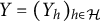
 $$ \begin{align} \Lambda^{\top} = \begin{pmatrix} \lambda_{11} & \lambda_{21} & 0 & \lambda_{41} & 0 & 0 \\ 0 & \lambda_{22} & \lambda_{32} & 0 & \lambda_{52} & 0 \\ 0 & 0 & \lambda_{33} & \lambda_{43} & 0 & \lambda_{63} \\ \end{pmatrix} \end{align} $$
is identifiable up to column sign in an almost sure sense, but the criterion of Anderson and Rubin (Reference Anderson and Rubin1956) and the subsequent developments are not able to certify it.
In contrast to prior work, we take a graphical perspective to specify the sparsity structure in $\Lambda $
(Lauritzen, Reference Lauritzen1996; Maathuis et al., Reference Maathuis, Drton, Lauritzen and Wainwright2019). For example, the graph in Figure 1 encodes the sparsity structure in the factor loading matrix given in Equation (2). When an edge
$\Lambda $
(Lauritzen, Reference Lauritzen1996; Maathuis et al., Reference Maathuis, Drton, Lauritzen and Wainwright2019). For example, the graph in Figure 1 encodes the sparsity structure in the factor loading matrix given in Equation (2). When an edge $h \rightarrow v$
is missing in the graph, the corresponding entry
$h \rightarrow v$
is missing in the graph, the corresponding entry $\lambda _{vh}$
is required to be zero. Building on Anderson and Rubin (Reference Anderson and Rubin1956) and Bekker and ten Berge (Reference Bekker and ten Berge1997), our new matching criterion (and an extension thereof) is a purely graphical criterion that exploits sparsity by operating locally on the structure of the graph.
$\lambda _{vh}$
is required to be zero. Building on Anderson and Rubin (Reference Anderson and Rubin1956) and Bekker and ten Berge (Reference Bekker and ten Berge1997), our new matching criterion (and an extension thereof) is a purely graphical criterion that exploits sparsity by operating locally on the structure of the graph.
Directed graph encoding the sparsity structure in a factor analysis model.

Figure 1 Long description
Starting at the top, three shaded nodes labeled h sub 1, h sub 2, and h sub 3 are positioned above six unshaded nodes labeled v sub 1 through v sub 6. H sub 1 connects downward with blue arrows to v sub 1, v sub 2, and v sub 3. H sub 2, located below h sub 1, connects upward with orange arrows to v sub 3, v sub 4, and v sub 5. H sub 3, at the top right, connects downward with green arrows to v sub 4, v sub 5, and v sub 6. Each arrow indicates a directed relationship from a hidden node to a visible node, encoding the sparsity structure of the factor analysis model.
Deciding identifiability corresponds to solving the equation system from (1). Since the equations are polynomial in the factor loadings $\lambda _{vh}$
, identifiability is, in principle, always decidable via Gröbner basis methods from computational algebraic geometry (Barber et al., Reference Barber, Drton, Sturma and Weihs2022; Garcia-Puente et al., Reference Garcia-Puente, Spielvogel and Sullivant2010). But the scope of such methods is limited to small graphs as their complexity can grow double exponentially with the size of the graph (Mayr, Reference Mayr1997). In contrast, our new graphical criteria can be checked in polynomial time, provided we restrict a search step to subsets of bounded size.
$\lambda _{vh}$
, identifiability is, in principle, always decidable via Gröbner basis methods from computational algebraic geometry (Barber et al., Reference Barber, Drton, Sturma and Weihs2022; Garcia-Puente et al., Reference Garcia-Puente, Spielvogel and Sullivant2010). But the scope of such methods is limited to small graphs as their complexity can grow double exponentially with the size of the graph (Mayr, Reference Mayr1997). In contrast, our new graphical criteria can be checked in polynomial time, provided we restrict a search step to subsets of bounded size.
The organization of the article is as follows. Section 2 formally introduces the concept of generic sign-identifiability, and we revisit the criteria of Anderson and Rubin (Reference Anderson and Rubin1956) and Bekker and ten Berge (Reference Bekker and ten Berge1997) in Section 3. Section 4 presents our main results, the matching criterion and its extension. In Section 5, we show that both criteria are decidable in polynomial time. In Section 6, we conduct experiments that demonstrate the performance of our criteria and exemplify how our identifiability criteria are also useful in exploratory factor analysis. The Supplementary Material contains additional results for full factor models (Appendix A of the Supplementary Material), efficient algorithms (Appendix B of the Supplementary Material), all technical proofs (Appendix C of the Supplementary Material), and an explanation of how to decide identifiability using algebraic tools (Appendix D of the Supplementary Material).
2 Graphical representation and identifiability
Let $G=(V \cup \mathcal {H}, D)$
be a directed graph, where V and
$G=(V \cup \mathcal {H}, D)$
be a directed graph, where V and $\mathcal {H}$
are finite disjoint sets of observed and latent nodes. We assume that the graph
$\mathcal {H}$
are finite disjoint sets of observed and latent nodes. We assume that the graph $G=(V \cup \mathcal {H}, D)$
is bipartite, that is, it only contains edges from latent to observed variables such that
$G=(V \cup \mathcal {H}, D)$
is bipartite, that is, it only contains edges from latent to observed variables such that $D \subseteq \mathcal {H} \times V$
. We refer to such graphs as factor analysis graphs. If G contains an edge
$D \subseteq \mathcal {H} \times V$
. We refer to such graphs as factor analysis graphs. If G contains an edge $(h,v) \in D$
, then we also denote this by
$(h,v) \in D$
, then we also denote this by $h \rightarrow v \in D$
. The set
$h \rightarrow v \in D$
. The set $\text {ch}(h)=\{v \in V: h \rightarrow v \in D\}$
contains the children of a latent node
$\text {ch}(h)=\{v \in V: h \rightarrow v \in D\}$
contains the children of a latent node $h \in \mathcal {H}$
, and the set
$h \in \mathcal {H}$
, and the set $\text {pa}(v)=\{h \in \mathcal {H}: h \rightarrow v \in D\}$
contains the parents of an observed node
$\text {pa}(v)=\{h \in \mathcal {H}: h \rightarrow v \in D\}$
contains the parents of an observed node $v \in V$
.
$v \in V$
.
Each bipartite graph defines a factor analysis model, which for our purposes may be identified with a set of covariance matrices.
Definition 2.1. Let $G=(V \cup \mathcal {H}, D)$
be a factor analysis graph with
$G=(V \cup \mathcal {H}, D)$
be a factor analysis graph with $|V|=p$
and
$|V|=p$
and $|\mathcal {H}|=m$
, and let
$|\mathcal {H}|=m$
, and let $\mathbb {R}^D$
be the space of real
$\mathbb {R}^D$
be the space of real $p\times m$
matrices
$p\times m$
matrices $\Lambda = (\lambda _{vh})$
with support D, that is,
$\Lambda = (\lambda _{vh})$
with support D, that is, $\lambda _{vh} = 0$
if
$\lambda _{vh} = 0$
if $h \rightarrow v \not \in D$
. The factor analysis model determined by G is the image
$h \rightarrow v \not \in D$
. The factor analysis model determined by G is the image $F(G) = \text {Im}(\tau _G)$
of the parameterization
$F(G) = \text {Im}(\tau _G)$
of the parameterization
 $$ \begin{align*} \begin{split} \tau_G : \mathbb{R}^p_{>0} \times \mathbb{R}^D &\longrightarrow \operatorname{\mathrm{\mathit{PD}}}(p) \\ (\Omega, \Lambda) &\longmapsto \Omega + \Lambda \Lambda^{\top}, \end{split} \end{align*} $$
where $\operatorname {\mathrm {\mathit {PD}}}(p)$
is the cone of positive-definite
$\operatorname {\mathrm {\mathit {PD}}}(p)$
is the cone of positive-definite $p \times p$
matrices, and
$p \times p$
matrices, and $\mathbb {R}^p_{>0} \subset \operatorname {\mathrm {\mathit {PD}}}(p)$
is the subset of diagonal positive-definite matrices.
$\mathbb {R}^p_{>0} \subset \operatorname {\mathrm {\mathit {PD}}}(p)$
is the subset of diagonal positive-definite matrices.
Identifiability holds if we can recover $\Omega $
and
$\Omega $
and $\Lambda $
from a given matrix
$\Lambda $
from a given matrix $\Sigma \in F(G)$
up to column signs of the matrix
$\Sigma \in F(G)$
up to column signs of the matrix $\Lambda $
. To make this precise, we write
$\Lambda $
. To make this precise, we write
 $$ \begin{align*}\mathcal{F}_G(\Omega, \Lambda) = \{(\widetilde{\Omega}, \widetilde{\Lambda}) \in \Theta_G : \tau_G(\widetilde{\Omega}, \widetilde{\Lambda}) = \tau_G(\Omega, \Lambda) \}\end{align*} $$
for the fiber of a pair $(\Omega , \Lambda )$
in the domain
$(\Omega , \Lambda )$
in the domain $\Theta _{G}=\mathbb {R}^{|V|}_{>0} \times \mathbb {R}^D$
of the parameterization
$\Theta _{G}=\mathbb {R}^{|V|}_{>0} \times \mathbb {R}^D$
of the parameterization $\tau _G$
.
$\tau _G$
.
Definition 2.2. A factor analysis graph $ G=(V \cup \mathcal {H}, D)$
is said to be generically sign-identifiable if
$ G=(V \cup \mathcal {H}, D)$
is said to be generically sign-identifiable if
 $$\begin{align*}\mathcal{F}_G(\Omega, \Lambda) = \{(\widetilde{\Omega}, \widetilde{\Lambda}) \in \Theta_G : \widetilde{\Omega} = \Omega \text{ and } \widetilde{\Lambda}=\Lambda \Psi \text{ for } \Psi \in \{\pm 1\}^{|\mathcal{H}| \times |\mathcal{H}|} \text{ diagonal}\} \end{align*}$$
for almost all $(\Omega , \Lambda ) \in \Theta _G$
. Moreover, we say that a node
$(\Omega , \Lambda ) \in \Theta _G$
. Moreover, we say that a node $h \in \mathcal {H}$
in a factor analysis graph
$h \in \mathcal {H}$
in a factor analysis graph $G=(V \cup \mathcal {H}, D)$
is generically sign-identifiable if it holds for almost all
$G=(V \cup \mathcal {H}, D)$
is generically sign-identifiable if it holds for almost all $(\Omega , \Lambda ) \in \Theta _G$
that each parameter pair
$(\Omega , \Lambda ) \in \Theta _G$
that each parameter pair $(\widetilde {\Omega }, \widetilde {\Lambda })\in \mathcal {F}_G(\Omega , \Lambda )$
satisfies
$(\widetilde {\Omega }, \widetilde {\Lambda })\in \mathcal {F}_G(\Omega , \Lambda )$
satisfies $\widetilde {\Lambda }_{\text {ch}(h),h}=\Lambda _{\text {ch}(h),h}$
.
$\widetilde {\Lambda }_{\text {ch}(h),h}=\Lambda _{\text {ch}(h),h}$
.
In Definition 2.2, “almost all” is meant with respect to the induced Lebesgue measure on $\Theta _G$
, considered as an open subset of
$\Theta _G$
, considered as an open subset of $\mathbb {R}^{|V|+|D|}$
. If a graph is generically sign-identifiable, then for a factor loading matrix
$\mathbb {R}^{|V|+|D|}$
. If a graph is generically sign-identifiable, then for a factor loading matrix $\Lambda $
and a diagonal covariance matrix
$\Lambda $
and a diagonal covariance matrix $\Omega $
drawn randomly from an absolutely continuous distribution, the resulting covariance matrix of the observable vector X will almost surely allow recovery of
$\Omega $
drawn randomly from an absolutely continuous distribution, the resulting covariance matrix of the observable vector X will almost surely allow recovery of $\Lambda $
up to column sign.
$\Lambda $
up to column sign.
Example 2.3. Consider the identification formula for $|\lambda _{11}|$
in Example 1.1 given by
$|\lambda _{11}|$
in Example 1.1 given by
 $$\begin{align*}\sqrt{\frac{\sigma_{13} \sigma_{14} }{\sigma_{34}}} = \sqrt{\frac{\lambda_{11}\lambda_{31} \, \lambda_{11}\lambda_{41}}{\lambda_{31}\lambda_{41}}}. \end{align*}$$
This formula does not hold if at least one of the parameters $\lambda _{31}$
and
$\lambda _{31}$
and $\lambda _{41}$
is equal to zero. Hence, for such exceptional parameter pairs
$\lambda _{41}$
is equal to zero. Hence, for such exceptional parameter pairs $(\Omega ,\Lambda ),$
we cannot establish the correct form of the fiber and identification fails. However, since the set of exceptional pairs forms a Lebesgue measure zero subset of the parameter space, we obtain generic sign-identifiability.
$(\Omega ,\Lambda ),$
we cannot establish the correct form of the fiber and identification fails. However, since the set of exceptional pairs forms a Lebesgue measure zero subset of the parameter space, we obtain generic sign-identifiability.
Note that any node h with $\text {ch}(h)=\emptyset $
is trivially generically sign-identifiable. For later reference, we formally record how generic sign-identifiability of the graph results from generic sign-identifiability of all nodes.
$\text {ch}(h)=\emptyset $
is trivially generically sign-identifiable. For later reference, we formally record how generic sign-identifiability of the graph results from generic sign-identifiability of all nodes.
Lemma 2.4. A factor analysis graph $G=(V \cup \mathcal {H}, D)$
is generically sign-identifiable if and only if all nodes
$G=(V \cup \mathcal {H}, D)$
is generically sign-identifiable if and only if all nodes $h \in \mathcal {H}$
are generically sign-identifiable.
$h \in \mathcal {H}$
are generically sign-identifiable.
Remark 2.5. A model can only be generically sign-identifiable if its dimension matches the parameter count $|V|+|D|$
. Recently, Drton et al. (Reference Drton, Grosdos, Portakal and Sturma2025) proved upper and lower bounds for the dimension of sparse factor analysis models. The bounds reveal that such models may have dimension strictly smaller than
$|V|+|D|$
. Recently, Drton et al. (Reference Drton, Grosdos, Portakal and Sturma2025) proved upper and lower bounds for the dimension of sparse factor analysis models. The bounds reveal that such models may have dimension strictly smaller than $|V|+|D|$
and, thus, may be non-identifiable. The bounds also show that a necessary condition for a factor analysis graph to be generically sign-identifiable is that each latent node has at least three children.
$|V|+|D|$
and, thus, may be non-identifiable. The bounds also show that a necessary condition for a factor analysis graph to be generically sign-identifiable is that each latent node has at least three children.
3 Existing criteria
Due to rotational indeterminacy, previous work on identifiability of full factor analysis models focused on identifying the diagonal matrix $\Omega $
. If we require that the upper triangle of the matrix
$\Omega $
. If we require that the upper triangle of the matrix $\Lambda $
is zero, then existing criteria may also yield generic sign-identifiability.
$\Lambda $
is zero, then existing criteria may also yield generic sign-identifiability.
Definition 3.1. A factor analysis graph $G=(V \cup \mathcal {H}, D)$
satisfies the zero upper triangular assumption (ZUTA) if there exists an ordering
$G=(V \cup \mathcal {H}, D)$
satisfies the zero upper triangular assumption (ZUTA) if there exists an ordering $\prec $
on the latent nodes
$\prec $
on the latent nodes $\mathcal {H}$
such that
$\mathcal {H}$
such that $\text {ch}(h)$
is not contained in
$\text {ch}(h)$
is not contained in $\bigcup _{\ell \succ h} \text {ch}(\ell )$
for all
$\bigcup _{\ell \succ h} \text {ch}(\ell )$
for all $h \in \mathcal {H}$
. In this case, we say that
$h \in \mathcal {H}$
. In this case, we say that $\prec $
is a ZUTA-ordering with respect to G.
$\prec $
is a ZUTA-ordering with respect to G.
ZUTA ensures that the rows and columns of the factor loading matrix $\Lambda $
can be permuted such that the upper triangle of the matrix is zero. Note that ZUTA eliminates rotational indeterminacy. That is, if it holds that
$\Lambda $
can be permuted such that the upper triangle of the matrix is zero. Note that ZUTA eliminates rotational indeterminacy. That is, if it holds that $\Sigma - \Omega = \widetilde {\Lambda } \widetilde {\Lambda }^{\top }$
for a matrix
$\Sigma - \Omega = \widetilde {\Lambda } \widetilde {\Lambda }^{\top }$
for a matrix $\widetilde {\Lambda }$
that is zero upper triangular, i.e.,
$\widetilde {\Lambda }$
that is zero upper triangular, i.e., $\widetilde {\Lambda }_{ij}=0$
for
$\widetilde {\Lambda }_{ij}=0$
for $i < j$
, then it follows from the uniqueness of the Cholesky decomposition that
$i < j$
, then it follows from the uniqueness of the Cholesky decomposition that $\widetilde {\Lambda }$
is unique up to column sign, i.e.,
$\widetilde {\Lambda }$
is unique up to column sign, i.e., $\widetilde {\Lambda } = \Lambda \Psi $
for a fixed matrix
$\widetilde {\Lambda } = \Lambda \Psi $
for a fixed matrix $\Lambda $
and a diagonal matrix
$\Lambda $
and a diagonal matrix $\Psi $
with entries in
$\Psi $
with entries in $\{\pm 1\}$
.
$\{\pm 1\}$
.
If a factor analysis graph satisfies the ZUTA condition, then there is an observed node $v_h \in \text {ch}(h)$
for each
$v_h \in \text {ch}(h)$
for each $h \in \mathcal {H}$
such that
$h \in \mathcal {H}$
such that $v_h \in \text {ch}(h)$
and
$v_h \in \text {ch}(h)$
and $v_h \not \in \bigcup _{\ell \succ h} \text {ch}(\ell )$
. In particular, it is a necessary condition for ZUTA that there is at least one observed node that only has one latent parent.
$v_h \not \in \bigcup _{\ell \succ h} \text {ch}(\ell )$
. In particular, it is a necessary condition for ZUTA that there is at least one observed node that only has one latent parent.
Example 3.2. The graph in Figure 2a satisfies ZUTA with the ordering $h_1 \prec h_2 \prec h_3$
, since
$h_1 \prec h_2 \prec h_3$
, since $v_4 \in \text {ch}(h_1)$
but
$v_4 \in \text {ch}(h_1)$
but $v_4 \not \in \text {ch}(h_2) \cup \text {ch}(h_3)$
, and
$v_4 \not \in \text {ch}(h_2) \cup \text {ch}(h_3)$
, and $v_3 \in \text {ch}(h_2)$
but
$v_3 \in \text {ch}(h_2)$
but $v_3 \not \in \text {ch}(h_3)$
. However, the graph in Figure 2b does not satisfy ZUTA as no observed node has only one parent.
$v_3 \not \in \text {ch}(h_3)$
. However, the graph in Figure 2b does not satisfy ZUTA as no observed node has only one parent.
Two factor analysis graphs. Graph (a) satisfies ZUTA while graph (b) does not.

Figure 2 Long description
Panel a contains three gray nodes labeled h sub 1, h sub 2, and h sub 3 at the top and bottom, with five white nodes labeled v sub 1 through v sub 5 in a row below. Blue arrows extend from h sub 1 to v sub 1, v sub 2, v sub 3, and v sub 4. Green arrows extend from h sub 1 to v sub 2 and from h sub 3 to v sub 5. Orange arrows extend from h sub 2 to v sub 1, v sub 3, and v sub 5. Panel b has the same node arrangement. Blue arrows from h sub 1 point to v sub 1, v sub 2, v sub 3, and v sub 4. Green arrows from h sub 1 point to v sub 2 and from h sub 3 to v sub 5. Orange arrows from h sub 2 point to v sub 1, v sub 3, v sub 4, and v sub 5. The difference is that in panel b, h sub 2 connects to v sub 4, which is absent in panel a.
Remark 3.3. ZUTA is equivalent to the generalized lower triangular assumption introduced in Frühwirth-Schnatter et al. (Reference Frühwirth-Schnatter, Hosszejni and Lopes2025), which operates directly on the matrix $\Lambda $
. ZUTA refers to the graph, which is useful to present our graphical criteria in Section 4.
$\Lambda $
. ZUTA refers to the graph, which is useful to present our graphical criteria in Section 4.
If we consider graphs that satisfy ZUTA, many criteria in the literature directly yield generic sign-identifiability. The most prominent condition for identifiability is still the criterion of Anderson and Rubin (Reference Anderson and Rubin1956). Since it is originally stated as a pointwise condition, it is also applicable to sparse graphs. To state the result one obtains, we treat the entries of $\Lambda $
as indeterminates and say that a submatrix is generically of rank k if it has rank k for almost all choices of
$\Lambda $
as indeterminates and say that a submatrix is generically of rank k if it has rank k for almost all choices of $\Lambda \in \mathbb {R}^D$
. Under the assumption that a graph satisfies ZUTA, Theorem 5.1 in Anderson and Rubin (Reference Anderson and Rubin1956) then translates to the following sufficient condition for generic sign-identifiability.
$\Lambda \in \mathbb {R}^D$
. Under the assumption that a graph satisfies ZUTA, Theorem 5.1 in Anderson and Rubin (Reference Anderson and Rubin1956) then translates to the following sufficient condition for generic sign-identifiability.
Theorem 3.4 (AR-identifiability)
Let $G=(V \cup \mathcal {H}, D)$
be a factor analysis graph that satisfies ZUTA. Then, G is generically sign-identifiable if for any deleted row of
$G=(V \cup \mathcal {H}, D)$
be a factor analysis graph that satisfies ZUTA. Then, G is generically sign-identifiable if for any deleted row of $\Lambda = (\lambda _{vh}) \in \mathbb {R}^D$
, there remain two disjoint submatrices that are generically of rank
$\Lambda = (\lambda _{vh}) \in \mathbb {R}^D$
, there remain two disjoint submatrices that are generically of rank $|\mathcal {H}|$
.
$|\mathcal {H}|$
.
If generic sign-identifiability can be proven by applying Theorem 3.4 for a factor analysis graph, then we say that the graph is AR-identifiable.
Example 3.5. The graph in Figure 3 gives rise to the transpose of $\Lambda \in \mathbb {R}^D$
given by
$\Lambda \in \mathbb {R}^D$
given by
 $$\begin{align*}\Lambda^{\top} = \begin{pmatrix} \lambda_{v_1 h_1} & \lambda_{v_2 h_1} & \lambda_{v_3 h_1} & \lambda_{v_4 h_1} & 0 \\ 0 & \lambda_{v_3 h_2} & \lambda_{v_3 h_2} & \lambda_{v_4 h_2} & \lambda_{v_5 h_2} \end{pmatrix}. \end{align*}$$
Deleting any row of $\Lambda $
leaves four rows that can always be split into two
$\Lambda $
leaves four rows that can always be split into two $2 \times 2$
matrices that generically have rank 2. Hence, the graph is AR-identifiable.
$2 \times 2$
matrices that generically have rank 2. Hence, the graph is AR-identifiable.
AR-identifiable factor analysis graph.

AR-identifiability requires $|V| \geq 2 |\mathcal {H}|+1$
. For general full factor analysis models, Bekker and ten Berge (Reference Bekker and ten Berge1997) solve the problem of generic identifiability (up to orthogonal transformation) in all but certain edge cases. However, the generic nature of their condition implies sign-identifiability results only for dense ZUTA graphs, in which only a permuted upper triangle vanishes.
$|V| \geq 2 |\mathcal {H}|+1$
. For general full factor analysis models, Bekker and ten Berge (Reference Bekker and ten Berge1997) solve the problem of generic identifiability (up to orthogonal transformation) in all but certain edge cases. However, the generic nature of their condition implies sign-identifiability results only for dense ZUTA graphs, in which only a permuted upper triangle vanishes.
Definition 3.6. A full-ZUTA graph is a factor analysis graph $G=(V \cup \mathcal {H}, D)$
that satisfies ZUTA but contains all other possible edges. That is, there is an ordering
$G=(V \cup \mathcal {H}, D)$
that satisfies ZUTA but contains all other possible edges. That is, there is an ordering $\prec $
on the latent nodes
$\prec $
on the latent nodes $\mathcal {H}=\{h_1, \ldots , h_m\}$
such that
$\mathcal {H}=\{h_1, \ldots , h_m\}$
such that $h_1 \prec \cdots \prec h_m$
, with the property that
$h_1 \prec \cdots \prec h_m$
, with the property that $\text {ch}(h_1)=V$
and
$\text {ch}(h_1)=V$
and $\text {ch}(h_{i+1})=\text {ch}(h_{i}) \setminus \{v_{i}\}$
for some child
$\text {ch}(h_{i+1})=\text {ch}(h_{i}) \setminus \{v_{i}\}$
for some child $v_{i} \in \text {ch}(h_{i})$
.
$v_{i} \in \text {ch}(h_{i})$
.
As an example, Figure 4a displays the full-ZUTA graph on three latent and six observed nodes. For full-ZUTA graphs, the criterion from Bekker and ten Berge (Reference Bekker and ten Berge1997) directly translates into the following sufficient condition for generic sign-identifiability.
Two full-ZUTA graphs.

Figure 4 Long description
Panel a on the left shows three hidden nodes labeled h sub 1, h sub 2, and h sub 3 at the top, and six visible nodes labeled v sub 1 through v sub 6 at the bottom. Blue arrows connect h sub 1 to v sub 1, v sub 2, v sub 3, v sub 4, v sub 5, and v sub 6. Orange arrows connect h sub 2 to v sub 2, v sub 3, v sub 4, v sub 5, and v sub 6. Green arrows connect h sub 3 to v sub 3, v sub 4, v sub 5, and v sub 6. Panel b on the right is similar but includes an additional visible node, v sub 7, at the far right. Blue arrows connect h sub 1 to v sub 1 through v sub 6. Orange arrows connect h sub 2 to v sub 2 through v sub 7. Green arrows connect h sub 3 to v sub 3 through v sub 7. All arrows point downward from hidden nodes to visible nodes.
Theorem 3.7 (BB-identifiability)
Let $G=(V \cup \mathcal {H}, D)$
be a full-ZUTA graph. Then, G is generically sign-identifiable if
$G=(V \cup \mathcal {H}, D)$
be a full-ZUTA graph. Then, G is generically sign-identifiable if $|V| + |D| < \binom {|V|+1}{2}$
.
$|V| + |D| < \binom {|V|+1}{2}$
.
If a full-ZUTA graph is generic sign-identifiability by Theorem 3.7, then we term the graph BB-identifiable. Note that $|V| + |D| = |V|(|\mathcal {H}|+1) - \binom {|\mathcal {H}|}{2}$
in a full-ZUTA graph. If
$|V| + |D| = |V|(|\mathcal {H}|+1) - \binom {|\mathcal {H}|}{2}$
in a full-ZUTA graph. If $|V| + |D|> \binom {|V|+1}{2}$
, then the parameter count is larger than the dimension of the ambient space of symmetric matrices, and full-ZUTA graphs are not generically sign-identifiable (recall Remark 2.5). Hence, the only remaining open cases where identifiability of full-ZUTA graphs is unknown are models “at the Ledermann bound,” where
$|V| + |D|> \binom {|V|+1}{2}$
, then the parameter count is larger than the dimension of the ambient space of symmetric matrices, and full-ZUTA graphs are not generically sign-identifiable (recall Remark 2.5). Hence, the only remaining open cases where identifiability of full-ZUTA graphs is unknown are models “at the Ledermann bound,” where $|V| + |D| = \binom {|V|+1}{2}$
.
$|V| + |D| = \binom {|V|+1}{2}$
.
Example 3.8. Figure 4 shows two full-ZUTA graphs. Graph (b) is BB-identifiable because $ |V| + |D| = 24 \, < \, 28 = \binom {7+1}{2}. $
Graph (a), on the other hand, has
$ |V| + |D| = 24 \, < \, 28 = \binom {7+1}{2}. $
Graph (a), on the other hand, has $ |V| + |D| = \, 21 \, = \binom {6+1}{2}. $
As already noted by Wilson and Worcester (Reference Wilson and Worcester1939), the fiber for graph (a), with
$ |V| + |D| = \, 21 \, = \binom {6+1}{2}. $
As already noted by Wilson and Worcester (Reference Wilson and Worcester1939), the fiber for graph (a), with $|V|=6$
and
$|V|=6$
and $|\mathcal {H}|=3$
, generically contains two diagonal matrices and two corresponding factor loading matrices together with their symmetries given by the sign changes of the columns.
$|\mathcal {H}|=3$
, generically contains two diagonal matrices and two corresponding factor loading matrices together with their symmetries given by the sign changes of the columns.
Remark 3.9. Generic sign-identifiability of full-ZUTA graphs does not imply identifiability of sparse subgraphs, since the models corresponding to subgraphs might be non-generic points in the model given by the full-ZUTA graph. For example, consider the full-ZUTA graph in Figure 5a that is generically sign-identifiable by Theorem 3.7. The graph in Figure 5b is a sparse subgraph. Since in this graph $|\text {ch}(h_2)| < 3$
, it follows that the model has not expected dimension and is hence not generically sign-identifiable (recall Remark 2.5).
$|\text {ch}(h_2)| < 3$
, it follows that the model has not expected dimension and is hence not generically sign-identifiable (recall Remark 2.5).
Full-ZUTA graph and a sparse subgraph.

The following example shows two graphs that are generically sign-identifiable but no known general criterion is able to certify it.
Example 3.10. The loading matrix for the graph in Figure 6 has transpose
 $$\begin{align*}\Lambda^{\top} = \begin{pmatrix} \lambda_{v_1 h_1} & \lambda_{v_2 h_1} & \lambda_{v_3 h_1} & \lambda_{v_4 h_1} & \lambda_{v_5 h_1} & \lambda_{v_6 h_1} & 0 & 0 & 0 \\ 0 & \lambda_{v_2 h_2} & \lambda_{v_3 h_2} & \lambda_{v_4 h_2} & \lambda_{v_5 h_2} & \lambda_{v_6 h_2} & 0 & 0 & 0 \\ 0 & 0 & \lambda_{v_3 h_3} & \lambda_{v_4 h_3} & \lambda_{v_5 h_3} & 0 & 0 & 0 & 0 \\ 0 & 0 & 0 & \lambda_{v_4 h_4} & 0 & \lambda_{v_6 h_4} & \lambda_{v_7 h_4} & \lambda_{v_8 h_4} & \lambda_{v_9 h_4} \end{pmatrix}. \end{align*}$$
The graph is not BB-identifiable as it is not full-ZUTA. To see that it is not AR-identifiable, delete the row of $\Lambda $
indexed by
$\Lambda $
indexed by $v_4$
. If we form two
$v_4$
. If we form two $4 \times 4$
-matrices out of the remaining eight rows, then one of these matrices has to contain at least two rows indexed by
$4 \times 4$
-matrices out of the remaining eight rows, then one of these matrices has to contain at least two rows indexed by $v_7$
,
$v_7$
, $v_8,$
or
$v_8,$
or $v_9$
. This matrix has at most rank three, which disproves AR-identifiability. Another example that is neither AR- nor BB-identifiable is the graph in Figure 1. Using the criteria we develop in the next section, we can certify identifiability of both graphs (see also Example 4.9).
$v_9$
. This matrix has at most rank three, which disproves AR-identifiability. Another example that is neither AR- nor BB-identifiable is the graph in Figure 1. Using the criteria we develop in the next section, we can certify identifiability of both graphs (see also Example 4.9).
Sparse factor analysis graphs that is not AR-identifiable nor BB-identifiable.

Figure 6 Long description
From left to right, hidden nodes h sub 1, h sub 2, h sub 3, and h sub 4 are shaded and positioned above visible nodes v sub 1 through v sub 9. h sub 1 connects to v sub 1, v sub 2, v sub 3, v sub 4, and v sub 5 with blue arrows. h sub 2 connects to v sub 3, v sub 4, and v sub 5 with orange arrows. h sub 3 connects to v sub 4 and v sub 5 with green arrows. h sub 4 connects to v sub 5, v sub 6, v sub 7, v sub 8, and v sub 9 with red arrows. Each arrow represents a directed sparse factor relationship from hidden to visible nodes.
Finally, we note that BB-identifiability subsumes AR-identifiability for full-ZUTA graphs.
Corollary 3.11. Let $G=(V \cup \mathcal {H}, D)$
be a full-ZUTA graph with
$G=(V \cup \mathcal {H}, D)$
be a full-ZUTA graph with $|\mathcal {H}|\geq 2$
latent nodes that is AR-identifiable. Then, G is also BB-identifiable.
$|\mathcal {H}|\geq 2$
latent nodes that is AR-identifiable. Then, G is also BB-identifiable.
However, there are full-ZUTA graphs that are BB- but not AR-identifiable. The smallest example has $|V|=8$
observed nodes and
$|V|=8$
observed nodes and $|\mathcal {H}|=4$
latent nodes.
$|\mathcal {H}|=4$
latent nodes.
4 Main identifiability results
In this section, we derive novel graphical criteria that are sufficient for generic sign-identifiability in sparse factor analysis graphs. As we will show, the criteria strictly generalize AR- and BB-identifiability for ZUTA graphs and are capable of certifying identifiability of models not covered by the AR- nor BB-criterion.
4.1 Matching criterion
Our first criterion takes the form of a recursive procedure and is based on a graphical extension of the Anderson–Rubin criterion that can be applied locally at a given node. In the AR criterion, for each observed node $v \in V$
, we need to find disjoint sets
$v \in V$
, we need to find disjoint sets $U,W \subseteq V\setminus \{v\}$
with
$U,W \subseteq V\setminus \{v\}$
with $|U|=|W|=|\mathcal {H}|$
such that
$|U|=|W|=|\mathcal {H}|$
such that $\det (\Lambda _{U,\mathcal {H}}) \neq 0$
and
$\det (\Lambda _{U,\mathcal {H}}) \neq 0$
and $\det (\Lambda _{W,\mathcal {H}}) \neq 0$
. This is equivalent to
$\det (\Lambda _{W,\mathcal {H}}) \neq 0$
. This is equivalent to $\det ([\Lambda \Lambda ^{\top }]_{U,W}) \neq 0$
. Our main idea is to derive, and locally apply, a modified version of the AR criterion that also considers sets
$\det ([\Lambda \Lambda ^{\top }]_{U,W}) \neq 0$
. Our main idea is to derive, and locally apply, a modified version of the AR criterion that also considers sets $U,W$
with cardinality smaller than
$U,W$
with cardinality smaller than $|\mathcal {H}|$
. In doing so, we need to ensure that
$|\mathcal {H}|$
. In doing so, we need to ensure that $\det ([\Lambda \Lambda ^{\top }]_{U,W}) \neq 0$
, i.e., we need to characterize when minors of
$\det ([\Lambda \Lambda ^{\top }]_{U,W}) \neq 0$
, i.e., we need to characterize when minors of $\Lambda \Lambda ^{\top }$
vanish. This can be achieved via the concept of trek separation (Sullivant et al., Reference Sullivant, Talaska and Draisma2010) and leads to the following definition.
$\Lambda \Lambda ^{\top }$
vanish. This can be achieved via the concept of trek separation (Sullivant et al., Reference Sullivant, Talaska and Draisma2010) and leads to the following definition.
Definition 4.1. Let $G=(V \cup \mathcal {H}, D)$
be a factor analysis graph, and let
$G=(V \cup \mathcal {H}, D)$
be a factor analysis graph, and let $A,B\subseteq V$
be two subsets of equal cardinality,
$A,B\subseteq V$
be two subsets of equal cardinality, $|A|=|B|=n$
. A matching of A and B is a system
$|A|=|B|=n$
. A matching of A and B is a system $\Pi = \{\pi _1, \ldots , \pi _n\}$
consisting of paths of the form
$\Pi = \{\pi _1, \ldots , \pi _n\}$
consisting of paths of the form
 $$\begin{align*}\pi_i: v_i \leftarrow h_i \rightarrow w_i, \quad i=1,\dots,n, \end{align*}$$
where all $h_i \in \mathcal {H}$
, and
$h_i \in \mathcal {H}$
, and $\{v_1, \ldots , v_n\}=A$
and
$\{v_1, \ldots , v_n\}=A$
and $\{w_1, \ldots , w_n\}=B$
. A matching is intersection-free if the
$\{w_1, \ldots , w_n\}=B$
. A matching is intersection-free if the $h_i$
are all distinct, and a matching avoids
$h_i$
are all distinct, and a matching avoids $\mathcal {L} \subseteq \mathcal {H}$
if
$\mathcal {L} \subseteq \mathcal {H}$
if $\mathcal {L} \cap \{h_1, \ldots , h_n\} = \emptyset $
.
$\mathcal {L} \cap \{h_1, \ldots , h_n\} = \emptyset $
.
Example 4.2. Consider the sets $A=\{v_2,v_3\}$
and
$A=\{v_2,v_3\}$
and $B=\{v_4,v_5\}$
in the graph from Figure 5a. The system
$B=\{v_4,v_5\}$
in the graph from Figure 5a. The system $ \{v_2 \leftarrow h_1 \rightarrow v_3, v_4 \leftarrow h_2 \rightarrow v_5\} $
is an intersection-free matching of A and B. If instead
$ \{v_2 \leftarrow h_1 \rightarrow v_3, v_4 \leftarrow h_2 \rightarrow v_5\} $
is an intersection-free matching of A and B. If instead $A=\{v_1,v_2,v_3\}$
and
$A=\{v_1,v_2,v_3\}$
and $B=\{v_1,v_4,v_5\}$
, then any matching between A and B has an intersection. An example is given by the set of paths
$B=\{v_1,v_4,v_5\}$
, then any matching between A and B has an intersection. An example is given by the set of paths $ \{v_1 \leftarrow h_1 \rightarrow v_1, v_2 \leftarrow h_1 \rightarrow v_3, v_4 \leftarrow h_2 \rightarrow v_5\} $
that intersects in the latent node
$ \{v_1 \leftarrow h_1 \rightarrow v_1, v_2 \leftarrow h_1 \rightarrow v_3, v_4 \leftarrow h_2 \rightarrow v_5\} $
that intersects in the latent node $h_1$
.
$h_1$
.
Our main tool is a lemma that considers determinants of submatrices of $\Lambda \Lambda ^{\top }$
for
$\Lambda \Lambda ^{\top }$
for $\Lambda \in \mathbb {R}^D$
. Here, we view the determinant as a polynomial in the indeterminates
$\Lambda \in \mathbb {R}^D$
. Here, we view the determinant as a polynomial in the indeterminates $\lambda _{vh}$
, that is, we view it as an algebraic object without reference to its evaluation at specific values.
$\lambda _{vh}$
, that is, we view it as an algebraic object without reference to its evaluation at specific values.
Lemma 4.3. Let $G=(V \cup \mathcal {H}, D)$
be a factor analysis graph, and let
$G=(V \cup \mathcal {H}, D)$
be a factor analysis graph, and let $\Lambda \in \mathbb {R}^D$
. For two subsets
$\Lambda \in \mathbb {R}^D$
. For two subsets $A, B \subseteq V$
of equal cardinality,
$A, B \subseteq V$
of equal cardinality, $\det ( [\Lambda \Lambda ^{\top }]_{A,B} )$
is not the zero polynomial if and only if there is an intersection-free matching of A and B.
$\det ( [\Lambda \Lambda ^{\top }]_{A,B} )$
is not the zero polynomial if and only if there is an intersection-free matching of A and B.
Applying Lemma 4.3 to Anderson and Rubin’s theorem yields the following corollary.
Corollary 4.4. Let $G=(V \cup \mathcal {H}, D)$
be a factor analysis graph that satisfies ZUTA. Then, G is AR-identifiable if and only if for all
$G=(V \cup \mathcal {H}, D)$
be a factor analysis graph that satisfies ZUTA. Then, G is AR-identifiable if and only if for all $v \in V$
, there exist two disjoint sets
$v \in V$
, there exist two disjoint sets $W,U \subseteq V \setminus \{v\}$
with
$W,U \subseteq V \setminus \{v\}$
with $|W|=|U|=|\mathcal {H}|$
such that there is an intersection-free matching between W and U.
$|W|=|U|=|\mathcal {H}|$
such that there is an intersection-free matching between W and U.
Example 4.5. We saw in Example 3.5 that the graph in Figure 3 is AR-identifiable. Corollary 4.4 allows us to certify AR-identifiability in a fully graphical way without relating to the factor loading matrix. For example, for node $v_5$
, we observe that the two sets
$v_5$
, we observe that the two sets $U=\{v_1,v_2\}$
and
$U=\{v_1,v_2\}$
and $W=\{v_3,v_4\}$
have intersection-free matching
$W=\{v_3,v_4\}$
have intersection-free matching $ \{v_1 \leftarrow h_1 \rightarrow v_2, v_3 \leftarrow h_2 \rightarrow v_4\}. $
Remark 4.6. The use of matchings to verify AR-identifiability also appears in recent work of Hosszejni and Frühwirth-Schnatter (Reference Hosszejni and Frühwirth-Schnatter2026, Proposition 2) who make a connection between computing classical maximal matchings in bipartite graphs and verifying AR-identifiability. They consider matchings that are defined on duplicate bipartite graphs, which are constructed by first duplicating all latent nodes of the original graph and then duplicating the edges connecting these new latent nodes to the original observed nodes. The criterion of Hosszejni and Frühwirth-Schnatter (Reference Hosszejni and Frühwirth-Schnatter2026) then establishes AR-identifiability by checking whether the duplicate bipartite graph admits a maximal matching that covers all latent nodes, both the original and their duplicates. However, this approach is not feasible when we modify Corollary 4.4 to be locally applicable, as we do next. The reason is that if not all latent nodes are part of the matching, we do not know a priori which nodes we should consider in the bipartite graph. Therefore, we consider intersection-free matchings defined with respect to the original factor analysis graph.
We are now ready to define our new matching criterion, which operates “node-wise” and considers generic sign-identifiability for individual latent nodes $h \in \mathcal {H}$
.
$h \in \mathcal {H}$
.
Definition 4.7. Fix a latent node $h \in \mathcal {H}$
in the factor analysis graph
$h \in \mathcal {H}$
in the factor analysis graph $G=(V \cup \mathcal {H}, D)$
. A tuple
$G=(V \cup \mathcal {H}, D)$
. A tuple $(v, W, U, S) \in V \times 2^{V} \times 2^{V} \times 2^{ \mathcal {H} \setminus \{h\}}$
satisfies the matching criterion with respect to h if
$(v, W, U, S) \in V \times 2^{V} \times 2^{V} \times 2^{ \mathcal {H} \setminus \{h\}}$
satisfies the matching criterion with respect to h if
-
(i) $\text {pa}(v)\setminus S = \{h\}$
and
$v \not \in W \cup U$
;
$\text {pa}(v)\setminus S = \{h\}$
and
$v \not \in W \cup U$
; -
(ii) W and U are disjoint, nonempty sets of equal cardinality;
-
(iii) there exists an intersection-free matching of W and U that avoids S;
-
(iv) there is no intersection-free matching of
$\{v\} \cup W$
and
$\{v\} \cup U$
that avoids S.


If $(v, W, U, S)$
satisfies the matching criterion with respect to h, then Condition (iii) ensures
$(v, W, U, S)$
satisfies the matching criterion with respect to h, then Condition (iii) ensures $\det ([\Lambda \Lambda ^{\top }]_{W,U}) \neq 0$
, and Condition (iv) ensures
$\det ([\Lambda \Lambda ^{\top }]_{W,U}) \neq 0$
, and Condition (iv) ensures $\det ([\Lambda \Lambda ^{\top }]_{\{v\} \cup W,\{v\} \cup U}) = 0$
after removing the nodes in S from the graph. The Laplace expansion of determinants then allows us to find a rational formula for
$\det ([\Lambda \Lambda ^{\top }]_{\{v\} \cup W,\{v\} \cup U}) = 0$
after removing the nodes in S from the graph. The Laplace expansion of determinants then allows us to find a rational formula for $\lambda _{vh}^2$
in terms of the entries of the covariance matrix. We can thus identify
$\lambda _{vh}^2$
in terms of the entries of the covariance matrix. We can thus identify $\lambda _{vh}$
up to sign. Having identified parameter
$\lambda _{vh}$
up to sign. Having identified parameter $\lambda _{v h}$
for one child
$\lambda _{v h}$
for one child $v \in \text {ch}(h)$
, it is easy to certify sign-identifiability of h, i.e., to identify the remaining parameters
$v \in \text {ch}(h)$
, it is easy to certify sign-identifiability of h, i.e., to identify the remaining parameters $\lambda _{uh}$
for
$\lambda _{uh}$
for $u \in \text {ch}(h) \setminus \{v\}$
up to the same sign. This is formalized in our first main result.
$u \in \text {ch}(h) \setminus \{v\}$
up to the same sign. This is formalized in our first main result.
Theorem 4.8 (M-identifiability)
Let $G=(V \cup \mathcal {H}, D)$
be a factor analysis graph, and fix a latent node
$G=(V \cup \mathcal {H}, D)$
be a factor analysis graph, and fix a latent node $h \in \mathcal {H}$
. Suppose that the tuple
$h \in \mathcal {H}$
. Suppose that the tuple $(v, W, U, S) \in V \times 2^{V} \times 2^{V} \times 2^{ \mathcal {H} \setminus \{h\}}$
satisfies the matching criterion with respect to h. If all nodes
$(v, W, U, S) \in V \times 2^{V} \times 2^{V} \times 2^{ \mathcal {H} \setminus \{h\}}$
satisfies the matching criterion with respect to h. If all nodes $\ell \in S$
are generically sign-identifiable, then h is generically sign-identifiable.
$\ell \in S$
are generically sign-identifiable, then h is generically sign-identifiable.
Theorem 4.8 provides a way to recursively certify generic sign-identifiability of a factor analysis graph by checking whether all nodes $h \in \mathcal {H}$
are generically sign-identifiable (recall Lemma 2.4). If generic sign-identifiability can be certified recursively by Theorem 4.8, then we call the factor analysis graph M-identifiable. The details of an efficient algorithm to check M-identifiability using max-flow techniques are described in Appendix B of the Supplementary Material.
$h \in \mathcal {H}$
are generically sign-identifiable (recall Lemma 2.4). If generic sign-identifiability can be certified recursively by Theorem 4.8, then we call the factor analysis graph M-identifiable. The details of an efficient algorithm to check M-identifiability using max-flow techniques are described in Appendix B of the Supplementary Material.
Example 4.9. The factor analysis graph in Figure 7 is not AR-identifiable since $|V|=2|\mathcal {H}|$
. However, it is M-identifiable. We recursively check all latent nodes
$|V|=2|\mathcal {H}|$
. However, it is M-identifiable. We recursively check all latent nodes $\mathcal {H} = \{ h_1, h_2, h_3 \}$
.
$\mathcal {H} = \{ h_1, h_2, h_3 \}$
.
-
h 1: Take
$v=v_1$
,
$S=\emptyset $
,
$U=\{v_2,v_6\}$
, and
$W=\{v_3,v_4\}$
. Conditions (i) and (ii) are easily checked, and for (iii), an intersection-free matching is given by
$\{v_2 \leftarrow h_1 \rightarrow v_3, v_6 \leftarrow h_2 \rightarrow v_4\}$
. To verify (iv), note that
$\text {pa}(\{v\} \cup U) \cap \text {pa}(\{v\} \cup W) = \{h_1, h_2\}$
, which implies that there cannot exist an intersection-free matching of
$\{v\} \cup U$
and
$\{v\} \cup W$
. -
h 2: Take
$v=v_2$
,
$S=\{h_1\}$
,
$U=\{v_3\}$
, and
$W=\{v_6\}$
. The matching
$\{v_3 \leftarrow h_2 \rightarrow v_6\}$
is intersection-free, and
$(\text {pa}(\{v\} \cup U) \cap \text {pa}(\{v\} \cup W)) \setminus S = \{h_2\}$
implies that (iv) holds. -
h 3: Take
$v=v_3$
,
$S=\{h_1,h_2\}$
,
$U=\{v_4\}$
, and
$W=\{v_5\}$
. The matching
$\{v_4 \leftarrow h_3 \rightarrow v_5\}$
is intersection-free, and
$(\text {pa}(\{v\} \cup U) \cap \text {pa}(\{v\} \cup W)) \setminus S = \{h_3\}$
implies that (iv) holds.


Note that the graphs in Figures 1 and 6 are also M-identifiable, which can be seen similarly.
M-identifiable sparse factor analysis graph.

Next, we show that M-identifiability subsumes AR-identifiability.
Corollary 4.10. Let $G=(V \cup \mathcal {H}, D)$
be a factor analysis graph that satisfies ZUTA. Then:
$G=(V \cup \mathcal {H}, D)$
be a factor analysis graph that satisfies ZUTA. Then:
-
(i) If G is AR-identifiable, then it is also M-identifiable.
-
(ii) If G is full-ZUTA, then G is AR-identifiable if and only if it is M-identifiable.
Even though M-identifiability subsumes AR-identifiability, it can also only establish identifiability of graphs that satisfy ZUTA.
Corollary 4.11. Let $G=(V \cup \mathcal {H}, D)$
be a factor analysis graph that is M-identifiable. Then, the factor analysis graph G satisfies ZUTA.
$G=(V \cup \mathcal {H}, D)$
be a factor analysis graph that is M-identifiable. Then, the factor analysis graph G satisfies ZUTA.
4.2 Extension of the matching criterion
By Corollary 4.10, M-identifiability subsumes AR-identifiability. However, it does not subsume BB-identifiability. For example, the full-ZUTA graph on $|V|=8$
observed nodes and
$|V|=8$
observed nodes and $|\mathcal {H}|=4$
latent nodes is BB- but not M-identifiable. We now provide a second criterion that can certify generic sign-identifiability of a set of latent nodes in a way that generalizes BB-identifiability. It operates by searching locally for full-ZUTA subgraphs
$|\mathcal {H}|=4$
latent nodes is BB- but not M-identifiable. We now provide a second criterion that can certify generic sign-identifiability of a set of latent nodes in a way that generalizes BB-identifiability. It operates by searching locally for full-ZUTA subgraphs $\widetilde {G}=(\widetilde {V}, \widetilde {D})$
that satisfy the condition
$\widetilde {G}=(\widetilde {V}, \widetilde {D})$
that satisfy the condition $|\widetilde {V}|+ |\widetilde {D}| < \binom {|\widetilde {V}|+1}{2}$
. Combining both criteria then yields an extension of the matching criterion. We start by defining the necessary concepts.
$|\widetilde {V}|+ |\widetilde {D}| < \binom {|\widetilde {V}|+1}{2}$
. Combining both criteria then yields an extension of the matching criterion. We start by defining the necessary concepts.
Definition 4.12. For a set $B \subseteq V$
of observed nodes, the set of joint parents of pairs in B is given by
$B \subseteq V$
of observed nodes, the set of joint parents of pairs in B is given by
 $$\begin{align*}\text{jpa}(B) = \{h \in \text{pa}(u) \cap \text{pa}(v): u,v \in B, u \neq v\}. \end{align*}$$
Moreover, for another set $S \subseteq V$
, we say that an ordering
$S \subseteq V$
, we say that an ordering $\prec $
on the set S is a B-first-ordering if, for two elements
$\prec $
on the set S is a B-first-ordering if, for two elements $v,w \in S$
, it holds that
$v,w \in S$
, it holds that $v \prec w$
whenever
$v \prec w$
whenever $v \in B \cap S$
and
$v \in B \cap S$
and $w \in S \setminus B$
.
$w \in S \setminus B$
.
Said differently, a B-first-ordering on a set of nodes S is a block-ordering such that all elements in B come first.
Example 4.13. Consider the graph in Figure 7, and let $B=\{v_1,v_2,v_3\}$
. The joint parents are given by
$B=\{v_1,v_2,v_3\}$
. The joint parents are given by $\text {jpa}(B)=\{h_1,h_2\}$
. Moreover, for
$\text {jpa}(B)=\{h_1,h_2\}$
. Moreover, for $S = \{v_1,v_2,v_4,v_5\}$
, an example of a B-first ordering is given by
$S = \{v_1,v_2,v_4,v_5\}$
, an example of a B-first ordering is given by $v_2 \prec v_1 \prec v_5 \prec v_4$
.
$v_2 \prec v_1 \prec v_5 \prec v_4$
.
We now define a criterion that generalizes BB-identifiability. For $A \subseteq V \cup \mathcal {H}$
, we write
$A \subseteq V \cup \mathcal {H}$
, we write $G[A]=(A,D_A)$
for the induced subgraph of
$G[A]=(A,D_A)$
for the induced subgraph of $G=(V \cup \mathcal {H}, D)$
. The edge set
$G=(V \cup \mathcal {H}, D)$
. The edge set $D_A=\{h \rightarrow v \in D: h, v \in A\}$
includes precisely those edges in D that have both endpoints in A.
$D_A=\{h \rightarrow v \in D: h, v \in A\}$
includes precisely those edges in D that have both endpoints in A.
Definition 4.14. Let $G=(V \cup \mathcal {H}, D)$
be a factor analysis graph. We say that the tuple
$G=(V \cup \mathcal {H}, D)$
be a factor analysis graph. We say that the tuple $(B, S) \in 2^V \times 2^{\mathcal {H}}$
satisfies the local BB-criterion if
$(B, S) \in 2^V \times 2^{\mathcal {H}}$
satisfies the local BB-criterion if
-
(i) the induced subgraph
$\widetilde {G} = G[B \cup (\text {jpa}(B)\setminus S)]$
is a full-ZUTA graph; -
(ii) for all
$h \in \text {jpa}(B)\setminus S$
, there is a B-first-ordering
$\prec _h$
on
$\text {ch}(h)$
such that for all
$v \in \text {ch}(h) \setminus B,$
there is
$u \in \text {ch}(h)$
with
$u \prec _h v$
and
$\text {jpa}(\{v,u\}) \setminus S \subseteq \{\ell \in \text {jpa}(B)\setminus S: \ell \preceq _{\text {ZUTA}} h \}$
, where
$\prec _{\text {ZUTA}}$
is the unique ZUTA-ordering on
$\text {jpa}(B)\setminus S$
induced by
$\widetilde {G}$
; -
(iii) for the edge set
$\widetilde {D}$
of the subgraph
$\widetilde {G}$
it holds that
$|B| + |\widetilde {D}| < \binom {|B|+1}{2}$
.


Theorem 4.15. Let $G=(V \cup \mathcal {H}, D)$
be a factor analysis graph and suppose that the tuple
$G=(V \cup \mathcal {H}, D)$
be a factor analysis graph and suppose that the tuple $(B,S)\in 2^V \times 2^{\mathcal {H}}$
satisfies the local BB-criterion. If all nodes
$(B,S)\in 2^V \times 2^{\mathcal {H}}$
satisfies the local BB-criterion. If all nodes $\ell \in S$
are generically sign-identifiable, then all nodes
$\ell \in S$
are generically sign-identifiable, then all nodes $h \in \text {jpa}(B)\setminus S$
are generically sign-identifiable.
$h \in \text {jpa}(B)\setminus S$
are generically sign-identifiable.
Similar to M-identifiability, Theorem 4.15 allows us to recursively certify generic sign-identifiability of a factor analysis graph by checking whether all nodes $h \in \mathcal {H}$
are generically sign-identifiable (recall Lemma 2.4).
$h \in \mathcal {H}$
are generically sign-identifiable (recall Lemma 2.4).
Example 4.16. We can use Theorem 4.15 to recursively certify generic sign-identifiability of all latent nodes of the graph displayed in Figure 8.
-
h 1, h 2: Take
$B=\{v_1, \ldots , v_5\}$
and
$S=\emptyset $
such that
$\text {jpa}(B)\setminus S = \{h_1,h_2\}$
. Observe that
$G[B \cup (\text {jpa}(B)\setminus S)]$
is a full-ZUTA graph such that Condition (iii) is satisfied. Note that the unique ZUTA-ordering on
$\text {jpa}(B)$
is given by
$h_1 \prec _{\text {ZUTA}} h_2$
, i.e., to verify Condition (ii), we proceed according to this ordering on the latent nodes. The only child of
$h_1$
that is not a member of B is
$v_7$
. Take any ordering
$\prec _{h_1}$
on
$\text {ch}(h_1)$
such that
$v_7$
is the largest node according to
$\prec _{h_1}$
. Then, the ordering
$\prec _{h_1}$
is a B-first-ordering and
$v_1 \prec _{h_1} v_7$
. Moreover, observe that
$\text {jpa}(\{v_1,v_7\}) = \{h_1\}$
. Similarly, we can take any ordering
$\prec _{h_2}$
on
$\text {ch}(h_2)$
such that
$v_6$
is the largest node according to
$\prec _{h_2}$
. Since
$\text {jpa}(\{v_1,v_6\}) = \{h_2\}$
, we conclude that Condition (ii) is satisfied. -
h 3, h 4: Take
$U=\{v_5, \ldots , v_9\}$
and
$S=\{h_1,h_2\}$
such that
$\text {jpa}(B)\setminus S = \{h_3,h_4\}$
. It is easy to verify that Conditions (i) and (iii) are satisfied. Moreover, we have that
$\text {ch}(h_i)\setminus B = \emptyset $
for
$i=3,4$
, that is, Condition (ii) is trivially satisfied.


On the other hand, each observed node in the graph in Figure 8 has at least two latent parents. This implies that ZUTA is not satisfied and hence, due to Corollary 4.11, the graph is not M-identifiable.
Graph that is certified to be generically sign-identifiable by Theorem 4.15.

Figure 8 Long description
Starting from the left, h sub 1 is at the top and h sub 2 is below. h sub 1 connects via blue arrows to v sub 1, v sub 2, v sub 3, v sub 4, and v sub 5. h sub 2 connects via orange arrows to v sub 1, v sub 2, v sub 3, v sub 4, v sub 5, and v sub 6. In the center, v sub 1 to v sub 6 are arranged horizontally. Moving right, h sub 3 is above h sub 4. h sub 3 connects via green arrows to v sub 6, v sub 7, v sub 8, and v sub 9. h sub 4 connects via red arrows to v sub 7, v sub 8, and v sub 9. All h nodes are shaded gray, v nodes are white, and arrows are colored to distinguish connection types.
Next, we show that the recursive application of Theorem 4.15 subsumes BB-identifiability, that is, we show equivalence on full-ZUTA graphs. Crucially, Theorem 4.15 is also able to certify generic sign-identifiability of sparse graphs.
Corollary 4.17. A full-ZUTA graph $G=(V \cup \mathcal {H}, D)$
is BB-identifiable if and only if generic sign-identifiability of G can be certified by recursively applying Theorem 4.15.
$G=(V \cup \mathcal {H}, D)$
is BB-identifiable if and only if generic sign-identifiability of G can be certified by recursively applying Theorem 4.15.
We obtain our final criterion by combining Theorems 4.8 and 4.15 iteratively in a recursive algorithm. We call a factor analysis graph extended M-identifiable if generic sign-identifiability can be certified recursively by Theorems 4.8 and 4.15 for all nodes $h \in \mathcal {H}$
. We have already seen in Example 4.16 that extended M-identifiability may also certify generic sign-identifiability of graphs not satisfying ZUTA. We now provide a further example, where we consider a graph that is extended M-identifiable but applying only one of Theorem 4.8 or Theorem 4.15 does not certify generic sign-identifiability.
$h \in \mathcal {H}$
. We have already seen in Example 4.16 that extended M-identifiability may also certify generic sign-identifiability of graphs not satisfying ZUTA. We now provide a further example, where we consider a graph that is extended M-identifiable but applying only one of Theorem 4.8 or Theorem 4.15 does not certify generic sign-identifiability.
Example 4.18. The factor analysis graph in Figure 9 is an extended M-identifiable. To see this, we recursively check all latent nodes $\mathcal {H}=\{h_1, \ldots , h_5\}$
.
$\mathcal {H}=\{h_1, \ldots , h_5\}$
.
-
h 5: The tuple
$(v,W,U,S)$
with
$v=v_{10}$
,
$S=\emptyset $
,
$U=\{v_7\},$
and
$W=\{v_9\}$
satisfies the matching criterion with respect to
$h_5$
. Conditions (i) and (ii) are easily checked, and for Condition (iii), an intersection-free matching is given by
$v_7 \leftarrow h_5 \rightarrow v_9$
. To verify Condition (iv), note that
$\text {pa}(\{v\} \cup U) \cap \text {pa}(\{v\} \cup W)=\{h_5\}$
, which implies that there cannot exist an intersection-free matching of
$\{v\} \cup U)$
and
$\{v\} \cup W$
. -
H ∖ h 5: The tuple
$(B,S)$
with
$B=\{v_1, \ldots , v_8\}$
and
$S=\{h_5\}$
satisfies the local BB-criterion and it holds that
$\text {jpa}(B)\setminus S = \mathcal {H} \setminus h_5$
. The induced subgraph
$G[B \cup \text {jpa}(B) \setminus S)]$
is a full-ZUTA graph on eight observed nodes and four latent nodes for which Condition (iii) holds. Since
$\text {ch}(h_i)\setminus B = \emptyset $
for
$i=1, \ldots , 4$
, Condition (ii) is trivially satisfied.


Extended M-identifiable sparse factor analysis graph.

Figure 9 Long description
At the top row are five shaded hidden nodes labeled h sub 1, h sub 2, h sub 3, h sub 4, and h sub 5, arranged left to right. Below them are ten unshaded visible nodes labeled v sub 1 through v sub 10, also arranged left to right. Arrows indicate directed connections: h sub 1 connects to v sub 1 through v sub 7 with blue arrows. h sub 2 connects to v sub 2 through v sub 7 with orange arrows. h sub 3 connects to v sub 4 through v sub 7 with green arrows. h sub 4 connects to v sub 5 through v sub 7 with red arrows. h sub 5 connects to v sub 7, v sub 8, v sub 9, and v sub 10 with black arrows. Each arrow points downward from a hidden node to its respective visible nodes, illustrating sparse factor relationships.
Finally, we emphasize that extended M-identifiability is only sufficient for generic sign-identifiability. Both graphs in Figure 10 can be shown to be generically sign-identifiable via techniques from computational algebra but are not extended M-identifiable.
Two generically sign-identifiable graphs that are not extended M-identifiable.

Figure 10 Long description
Panel a on the left displays h sub 1, h sub 2, and h sub 3 at the top, with v sub 1 through v sub 6 below. Blue arrows from h sub 1 point to v sub 1, v sub 2, v sub 4, and v sub 6. Orange arrows from h sub 2 point to v sub 2, v sub 4, and v sub 6. Green arrows from h sub 3 point to v sub 3, v sub 4, v sub 5, and v sub 6. Panel b on the right shows the same node arrangement. Blue arrows from h sub 1 point to v sub 1, v sub 2, v sub 4, and v sub 6. Orange arrows from h sub 2 point to v sub 2, v sub 4, v sub 5, and v sub 6. Green arrows from h sub 3 point to v sub 3, v sub 4, v sub 5, and v sub 6. The main difference is that in panel b, h sub 2 has an additional arrow to v sub 5 compared to panel a.
5 Computation
M-identifiability and extended M-identifiability are decidable in polynomial time under certain bounds on the sizes of the subsets involved. In Appendix B of the Supplementary Material, we detail efficient algorithms that are sound and complete.
Theorem 5.1. M-identifiability of a factor analysis graph $G=(V \cup \mathcal {H}, D)$
is decidable in time
$G=(V \cup \mathcal {H}, D)$
is decidable in time $\mathcal {O}(|\mathcal {H}|^{2} |V|^{k+1} (|V|+|\mathcal {H}|)^3)$
if we only allow sets W with
$\mathcal {O}(|\mathcal {H}|^{2} |V|^{k+1} (|V|+|\mathcal {H}|)^3)$
if we only allow sets W with $|W| \leq k$
in the matching criterion.
$|W| \leq k$
in the matching criterion.
Proof. See Theorem B.4 and Algorithm 2 in the Supplementary Material.
Theorem 5.2. Extended M-identifiability of a factor analysis graph $G=(V \cup \mathcal {H}, D)$
is decidable in time
$G=(V \cup \mathcal {H}, D)$
is decidable in time $\mathcal {O}(|\mathcal {H}|^2|V|^{\max \{k,l\}+1} (|V|+|\mathcal {H}|)^3)$
if we only allow sets W with
$\mathcal {O}(|\mathcal {H}|^2|V|^{\max \{k,l\}+1} (|V|+|\mathcal {H}|)^3)$
if we only allow sets W with $|W| \leq k$
in the matching criterion and only sets B with
$|W| \leq k$
in the matching criterion and only sets B with $|B| \leq \ell $
in the local BB-criterion.
$|B| \leq \ell $
in the local BB-criterion.
Proof. See Theorem B.8 and Algorithm 6 in the Supplementary Material.
If we allow the cardinality of the sets to be unbounded, then the algorithms we propose in the Supplementary Material search over an exponentially large space and, thus, may take exponential time in the number of nodes. We conjecture that one cannot do significantly better.
Conjecture 5.3. Deciding M-identifiability and extended M-identifiability both is NP-complete.
Remark 5.4. In practice, if there are no restrictions in terms of computational time, then we can allow sets W and B of arbitrary size. In this case, Algorithm 6 in the Supplementary Material is sound and complete for deciding extended M-identifiability of a latent-factor graph. That is, it returns “yes” if and only if the input graph is extended M-identifiable (see Theorem B.8 in the Supplementary Material). However, the run-time of the unconstrained algorithm is exponential in the number of nodes of the graph. Note that allowing sets of W and B of unconstrained size is equivalent to choosing $k=|\mathcal {H}|$
and
$k=|\mathcal {H}|$
and $\ell =|V|$
since
$\ell =|V|$
since $|W|\leq |\mathcal {H}|$
and
$|W|\leq |\mathcal {H}|$
and $|B|\leq |V|$
according to the definitions of the matching criterion and the local BB-criterion. Choosing smaller maximal sizes k and
$|B|\leq |V|$
according to the definitions of the matching criterion and the local BB-criterion. Choosing smaller maximal sizes k and $\ell $
can be useful in practice when attempting to verify generic sign-identifiability of large graphs, where the unconstrained version of Algorithm 6 in the Supplementary Material does not terminate in a reasonable amount of time. With
$\ell $
can be useful in practice when attempting to verify generic sign-identifiability of large graphs, where the unconstrained version of Algorithm 6 in the Supplementary Material does not terminate in a reasonable amount of time. With $k<|\mathcal {H}|$
and
$k<|\mathcal {H}|$
and $\ell < |V|$
, Algorithm 6 in the Supplementary Material is sound but not complete. That is, if the algorithm returns “yes” with
$\ell < |V|$
, Algorithm 6 in the Supplementary Material is sound but not complete. That is, if the algorithm returns “yes” with $k<|\mathcal {H}|$
and
$k<|\mathcal {H}|$
and $\ell < |V|$
, then extended M-identifiability holds, which in turn implies generic sign-identifiability. In this case, during the recursive computations, every tuple certified to satisfy the matching criterion fulfills
$\ell < |V|$
, then extended M-identifiability holds, which in turn implies generic sign-identifiability. In this case, during the recursive computations, every tuple certified to satisfy the matching criterion fulfills $|W|\leq k$
, and every tuple certified to satisfy the local BB-criterion fulfills
$|W|\leq k$
, and every tuple certified to satisfy the local BB-criterion fulfills $|B|\leq \ell $
. However, if the algorithm returns “no” with
$|B|\leq \ell $
. However, if the algorithm returns “no” with $k<|\mathcal {H}|$
and
$k<|\mathcal {H}|$
and $\ell < |V|$
, then we remain inconclusive whether the input graph is extended M-identifiable.
$\ell < |V|$
, then we remain inconclusive whether the input graph is extended M-identifiable.
Remark 5.5. Hosszejni and Frühwirth-Schnatter (Reference Hosszejni and Frühwirth-Schnatter2026) provide an efficient method to check AR-identifiability in polynomial time by computing maximal matchings in a bipartite graph. As explained in Remark 4.6, their approach is infeasible for checking our matching criterion, as it is a local version of AR-identifiability. The reason why the matching criterion is significantly more computationally intensive is as follows. Recall from Corollary 4.4 that a factor analysis graph that satisfies ZUTA is AR-identifiable if and only if, for all $v \in V$
, there exist two disjoint sets
$v \in V$
, there exist two disjoint sets $W,U \subseteq V \setminus \{v\}$
with
$W,U \subseteq V \setminus \{v\}$
with $|W|=|U|=|\mathcal {H}|$
and an intersection-free matching between W and U. The crucial difference to Condition (iii) in the matching criterion is that it is already known a priori that the intersection-free matching will involve all nodes
$|W|=|U|=|\mathcal {H}|$
and an intersection-free matching between W and U. The crucial difference to Condition (iii) in the matching criterion is that it is already known a priori that the intersection-free matching will involve all nodes $h \in \mathcal {H}$
. Checking Condition (iii) in the matching criterion can be seen as checking AR-identifiability locally for every possible subset of latent variables
$h \in \mathcal {H}$
. Checking Condition (iii) in the matching criterion can be seen as checking AR-identifiability locally for every possible subset of latent variables $H \subseteq \mathcal {H}$
. Moreover, the matching criterion needs the additional Condition (iv) to avoid an intersection-free matching between
$H \subseteq \mathcal {H}$
. Moreover, the matching criterion needs the additional Condition (iv) to avoid an intersection-free matching between $\{v\} \cup W$
and
$\{v\} \cup W$
and $\{v\} \cup U$
. This is not needed for AR-identifiability because the existence of such a matching is impossible if
$\{v\} \cup U$
. This is not needed for AR-identifiability because the existence of such a matching is impossible if $|W|=|U|=|\mathcal {H}|$
.
$|W|=|U|=|\mathcal {H}|$
.
6 Numerical experiments
In this section, we first conduct simulations that demonstrate the performance of our criteria. Then, we exemplify how our identifiability criteria are also useful in exploratory factor analysis.
Counts of unlabeled sparse factor graphs satisfying ZUTA with at most $|V|=7$
observed nodes and
$|V|=7$
observed nodes and $|\mathcal {H}|=3$
latent nodes
$|\mathcal {H}|=3$
latent nodes

Table 1 Long description
The table has six columns. The first column lists the number of edges, ranging from 1 to 18, plus a total row. The next five columns are labeled ZUTA, gen. sign-id, AR-id, M-id, and Ext. M-id. For each row, the counts are as follows: for 1 edge, ZUTA is 1, all others are 0; for 2 edges, ZUTA is 2, all others are 0; for 3 edges, ZUTA is 4, the rest are 1; for 4 edges, ZUTA is 7, the rest are 1; for 5 edges, ZUTA is 14, the rest are 1; for 6 edges, ZUTA is 25, the rest are 3; for 7 edges, ZUTA is 41, the rest are 4; for 8 edges, ZUTA is 56, the rest are 6; for 9 edges, ZUTA is 73, gen. sign-id is 8, AR-id is 7, M-id and Ext. M-id are 8; for 10 edges, ZUTA is 77, gen. sign-id is 11, AR-id is 9, M-id and Ext. M-id are 11; for 11 edges, ZUTA is 79, gen. sign-id is 23, AR-id is 16, M-id and Ext. M-id are 23; for 12 edges, ZUTA is 67, gen. sign-id is 31, AR-id is 23, M-id and Ext. M-id are 29; for 13 edges, ZUTA is 54, gen. sign-id is 33, AR-id is 29, M-id and Ext. M-id are 33; for 14 edges, ZUTA is 31, gen. sign-id is 23, AR-id is 21, M-id and Ext. M-id are 23; for 15 edges, ZUTA is 18, gen. sign-id, AR-id, M-id and Ext. M-id are 16; for 16 edges, ZUTA is 8, the rest are 8; for 17 edges, ZUTA is 4, the rest are 4; for 18 edges, ZUTA is 1, the rest are 1. The total row sums to ZUTA 562, gen. sign-id 174, AR-id 150, M-id and Ext. M-id 172.
6.1 Simulations
In our simulations, we compare different criteria for generic sign-identifiability. We treat graphs as unlabeled, that is, we count isomorphism classes of graphs. Two factor analysis graphs $G=(V \cup \mathcal {H}, D)$
and
$G=(V \cup \mathcal {H}, D)$
and $G'=(V \cup \mathcal {H}, D')$
on the same set of nodes are isomorphic if there is a permutation
$G'=(V \cup \mathcal {H}, D')$
on the same set of nodes are isomorphic if there is a permutation $\pi _V$
on the observed nodes V and a permutation
$\pi _V$
on the observed nodes V and a permutation $\pi _{\mathcal {H}}$
on the latent nodes
$\pi _{\mathcal {H}}$
on the latent nodes $\mathcal {H}$
such that, for
$\mathcal {H}$
such that, for $h \in \mathcal {H}$
and
$h \in \mathcal {H}$
and $v \in V$
, the edge
$v \in V$
, the edge $h \rightarrow v \in D$
if and only if
$h \rightarrow v \in D$
if and only if $\pi _{\mathcal {H}}(h) \rightarrow \pi _{V}(v) \in D'$
.
$\pi _{\mathcal {H}}(h) \rightarrow \pi _{V}(v) \in D'$
.
Counts of unlabeled sparse factor graphs with at most $|V|=9$
observed nodes and
$|V|=9$
observed nodes and $|\mathcal {H}|=4$
latent nodes
$|\mathcal {H}|=4$
latent nodes

Table 2 Long description
The table has six columns. The first column, Number of edges, ranges from 1 to greater than 30, plus a Total row. The next five columns are Total, ZUTA, AR-id, M-id, and Ext. M-id. For 1 edge, the counts are 1 for Total and ZUTA, 0 for the rest. For 2 edges, 3 for Total, 2 for ZUTA, 0 for others. For 3 edges, 6 Total, 4 ZUTA, 1 each for AR-id, M-id, Ext. M-id. For 4 edges, 16 Total, 8 ZUTA, 1 each for AR-id, M-id, Ext. M-id. For 5 edges, 27 Total, 16 ZUTA, 1 each for AR-id, M-id, Ext. M-id. For 6 edges, 62 Total, 34 ZUTA, 3 each for AR-id, M-id, Ext. M-id. For 7 edges, 111 Total, 71 ZUTA, 4 each for AR-id, M-id, Ext. M-id. For 8 edges, 225 Total, 146 ZUTA, 9 each for AR-id, M-id, Ext. M-id. For 9 edges, 395 Total, 287 ZUTA, 14 AR-id, 15 each for M-id and Ext. M-id. For 10 edges, 716 Total, 528 ZUTA, 21 AR-id, 23 each for M-id and Ext. M-id. For 11 edges, 1,165 Total, 922 ZUTA, 43 AR-id, 50 each for M-id and Ext. M-id. For 12 edges, 1,880 Total, 1,504 ZUTA, 81 AR-id, 93 each for M-id and Ext. M-id. For 13 edges, 2,726 Total, 2,273 ZUTA, 134 AR-id, 167 each for M-id and Ext. M-id. For 14 edges, 3,829 Total, 3,192 ZUTA, 221 AR-id, 366 M-id, 368 Ext. M-id. For 15 edges, 4,890 Total, 4,147 ZUTA, 404 AR-id, 768 each for M-id and Ext. M-id. For 16 edges, 5,963 Total, 4,972 ZUTA, 759 AR-id, 1,430 M-id, 1,435 Ext. M-id. For 17 edges, 6,599 Total, 5,490 ZUTA, 1,299 AR-id, 2,187 M-id, 2,204 Ext. M-id. For 18 edges, 6,937 Total, 5,519 ZUTA, 1,927 AR-id, 2,861 M-id, 2,913 Ext. M-id. For 19 edges, 6,599 Total, 5,047 ZUTA, 2,385 AR-id, 3,164 M-id, 3,273 Ext. M-id. For 20 edges, 5,963 Total, 4,191 ZUTA, 2,509 AR-id, 3,037 M-id, 3,179 Ext. M-id. For 21 edges, 4,890 Total, 3,157 ZUTA, 2,231 AR-id, 2,520 M-id, 2,656 Ext. M-id. For 22 edges, 3,829 Total, 2,139 ZUTA, 1,705 AR-id, 1,833 M-id, 1,913 Ext. M-id. For 23 edges, 2,726 Total, 1,310 ZUTA, 1,128 AR-id, 1,177 M-id, 1,215 Ext. M-id. For 24 edges, 1,880 Total, 710 ZUTA, 651 AR-id, 665 M-id, 683 Ext. M-id. For 25 edges, 1,165 Total, 343 ZUTA, 328 AR-id, 331 M-id, 344 Ext. M-id. For 26 edges, 716 Total, 153 ZUTA, 151 AR-id, 151 M-id, 155 Ext. M-id. For 27 edges, 395 Total, 64 ZUTA, 64 AR-id, 64 M-id, 65 Ext. M-id. For 28 edges, 225 Total, 22 ZUTA, 22 AR-id, 22 M-id, 22 Ext. M-id. For 29 edges, 111 Total, 7 ZUTA, 7 AR-id, 7 M-id, 7 Ext. M-id. For 30 edges, 62 Total, 1 ZUTA, 1 AR-id, 1 M-id, 1 Ext. M-id. For more than 30 edges, 54 Total, 0 for all others. The final row sums to 64,166 Total, 46,260 ZUTA, 16,104 AR-id, 20,951 M-id, and 21,568 Ext. M-id.
In our first experimental setup, we consider factor analysis graphs with a small number of observed and latent nodes where generic sign-identifiability can be fully solved by methods from computational algebraic geometry, as we discuss in Appendix D of the Supplementary Material. Table 1 lists counts of all factor analysis graphs with up to three latent nodes and seven observed nodes that satisfy ZUTA. We count how many of the graphs are AR-identifiable, M-identifiable, and extended M-identifiable. For deciding AR-identifiability, we use the algorithm and code provided by Hosszejni and Frühwirth-Schnatter (Reference Hosszejni and Frühwirth-Schnatter2026). Note that our criteria are very effective since we only fail to certify the generic sign-identifiability of two graphs. Those are exactly the graphs displayed in Figure 10. Table 1 also illustrates that M-identifiability subsumes AR-identifiability as we have shown in Corollary 4.10. On the other hand, M-identifiability and extended M-identifiability coincide on the considered set of small graphs. This is as expected since the smallest graph, where BB-identifiability holds but M-identifiability does not, has eight observed nodes and four latent nodes.
Our second experimental setup considers all factor analysis graphs with up to four latent nodes and nine observed nodes, and also includes graphs that do not satisfy ZUTA. Table 2 shows that the gap between AR-identifiability and M-identifiability increases. Moreover, extended M-identifiability indeed becomes effective since there are 617 graphs that are extended M-identifiable but not M-identifiable. Recall also that graphs not satisfying ZUTA might be extended M-identifiable but they are never M-identifiable nor AR-identifiable. For computational reasons, we are not able to fully solve generic sign-identifiability by methods from computational algebraic geometry for all graphs considered in Table 2.
Next, to demonstrate that checking extended M-identifiability is feasible on larger graphs with more observed and latent nodes, we randomly generate graphs on $25$
observed nodes and
$25$
observed nodes and $10$
latent nodes. We draw the graphs from an Erdös–Renyi model with edge probabilities
$10$
latent nodes. We draw the graphs from an Erdös–Renyi model with edge probabilities $0.2$
,
$0.2$
, $0.25$
,
$0.25$
, $0.3$
,
$0.3$
, $0.35$
,
$0.35$
, $0.4$
, and
$0.4$
, and $0.45$
, where we fix the upper triangle of the adjacency matrix to zero to increase the probability of satisfying ZUTA. Moreover, we only consider graphs with at most
$0.45$
, where we fix the upper triangle of the adjacency matrix to zero to increase the probability of satisfying ZUTA. Moreover, we only consider graphs with at most $10$
children per latent node such that the maximal cardinality of a set B satisfying the local BB-criterion is at most
$10$
children per latent node such that the maximal cardinality of a set B satisfying the local BB-criterion is at most $10$
. For each edge probability, we sample
$10$
. For each edge probability, we sample $5,000$
graphs and check whether they are extended M-identifiable. When searching for sets that satisfy the matching criterion, we bound the size of set W by
$5,000$
graphs and check whether they are extended M-identifiable. When searching for sets that satisfy the matching criterion, we bound the size of set W by $k=4$
. The number of graphs that were extended M-identifiable is reported in Table 3. Recall that only graphs with at least three children per latent node can be extended M-identifiable. For low edge probabilities, the likelihood is high that this is not satisfied. As expected, the fraction of extended M-identifiable graphs increases with increasing edge probabilities. However, at a certain density level, we would expect that fewer graphs are extended M-identifiable, which we can already see for the edge probability
$k=4$
. The number of graphs that were extended M-identifiable is reported in Table 3. Recall that only graphs with at least three children per latent node can be extended M-identifiable. For low edge probabilities, the likelihood is high that this is not satisfied. As expected, the fraction of extended M-identifiable graphs increases with increasing edge probabilities. However, at a certain density level, we would expect that fewer graphs are extended M-identifiable, which we can already see for the edge probability $p=0.45$
.
$p=0.45$
.
Status of extended M-identifiability for 5,000 randomly generated sparse factor graphs with different edge probabilities with $|W|\leq k$
for
$|W|\leq k$
for $k=4$
$k=4$

Table 3 Long description
The table has six columns for edge probabilities: 0.2, 0.25, 0.3, 0.35, 0.4, and 0.45. For each probability, the first row lists the count of extended M-identifiable graphs out of 5,000: 510 at 0.2, 1,784 at 0.25, 3,234 at 0.3, 4,184 at 0.35, 4,536 at 0.4, and 4,498 at 0.45. The second row gives the corresponding percentages: 10.2 percent, 35.7 percent, 64.7 percent, 83.7 percent, 90.7 percent, and 90.0 percent. The data shows a monotonic increase in both count and percentage of extended M-identifiable graphs as edge probability increases, peaking at 0.4 before a slight decrease at 0.45.
6.2 Application to exploratory factor analysis
In this section, we discuss how our identifiability criteria are also useful in exploratory factor analysis. It is a desirable property in exploratory factor analysis to discover a sparse structure that yields interpretable factor loadings. If we apply threshold-based sparse estimation methods, for example, our identifiability criteria can provide guidance in choosing the threshold or tuning parameter such that identifiability is ensured.
To exemplify this in a small case study, we consider the 2018 Populism and Political Parties Expert Survey (POPPA) that measures positions and attitudes of 250 parties on key attributes related to populism, political style, party ideology, and party organization (Meijers & Zaslove, Reference Meijers and Zaslove2020). The data set is obtained from an expert survey in 28 European countries and contains $|V|=15$
measured variables. After discarding data points with missing values,
$|V|=15$
measured variables. After discarding data points with missing values, $220$
samples remain. In their analyses of the data, Meijers and Zaslove (Reference Meijers and Zaslove2021) also conduct an exploratory factor analysis. While they retain two latent factors in the main manuscript, they also consider five factors in the Supplementary Material. We replicate their study with five factors by first estimating the loading matrix via maximum likelihood and then applying varimax rotation (Kaiser, Reference Kaiser1958) using the factanal function in the base library of R (R Core Team, 2025). We then set all loadings smaller than a predefined threshold to zero to obtain a sparse loading matrix
$220$
samples remain. In their analyses of the data, Meijers and Zaslove (Reference Meijers and Zaslove2021) also conduct an exploratory factor analysis. While they retain two latent factors in the main manuscript, they also consider five factors in the Supplementary Material. We replicate their study with five factors by first estimating the loading matrix via maximum likelihood and then applying varimax rotation (Kaiser, Reference Kaiser1958) using the factanal function in the base library of R (R Core Team, 2025). We then set all loadings smaller than a predefined threshold to zero to obtain a sparse loading matrix $\Lambda $
. The associated factor analysis graph includes edge
$\Lambda $
. The associated factor analysis graph includes edge $h \rightarrow v \in D$
if and only if
$h \rightarrow v \in D$
if and only if $\lambda _{hv} \neq 0$
. Note that we do not analyze the two-factor model because generic sign-identifiability is readily ensured as long as at least one measurement does not load on both factors, making the five-factor model a more illustrative setting.
$\lambda _{hv} \neq 0$
. Note that we do not analyze the two-factor model because generic sign-identifiability is readily ensured as long as at least one measurement does not load on both factors, making the five-factor model a more illustrative setting.
In their analysis, Meijers and Zaslove (Reference Meijers and Zaslove2021) use a threshold of $0.5$
, which yields a very sparse graph with some factors having less than three children, and thus generic sign-identifiability does not hold (recall Remark 2.5). In contrast, we check whether extended M-identifiability holds for graphs obtained from different thresholds. We obtain that extended M-identifiability only holds for thresholds in the interval
$0.5$
, which yields a very sparse graph with some factors having less than three children, and thus generic sign-identifiability does not hold (recall Remark 2.5). In contrast, we check whether extended M-identifiability holds for graphs obtained from different thresholds. We obtain that extended M-identifiability only holds for thresholds in the interval $[0.10, 0.14]$
. Note that ZUTA is not satisfied for the graphs given by all thresholds in this interval, while it is satisfied for all graphs obtained from thresholds
$[0.10, 0.14]$
. Note that ZUTA is not satisfied for the graphs given by all thresholds in this interval, while it is satisfied for all graphs obtained from thresholds $\geq $
0.15. In Table 4, we plot the factor loading matrix that we obtain for the threshold
$\geq $
0.15. In Table 4, we plot the factor loading matrix that we obtain for the threshold $0.10$
. Meijers and Zaslove (Reference Meijers and Zaslove2021) argue that the first latent factor represents populism since the first five measurements were designed to measure populism and load strongly on it. For more information on the measured variables, we refer to Meijers and Zaslove (Reference Meijers and Zaslove2021).
$0.10$
. Meijers and Zaslove (Reference Meijers and Zaslove2021) argue that the first latent factor represents populism since the first five measurements were designed to measure populism and load strongly on it. For more information on the measured variables, we refer to Meijers and Zaslove (Reference Meijers and Zaslove2021).
Factor loading matrix obtained via maximum likelihood estimation and varimax rotation from the POPPA data set

Table 4 Long description
The table presents a factor loading matrix with 15 rows labeled 1 to 15 and five columns labeled Factor 1 through Factor 5. For each item, loadings are listed under each factor, with some cells blank if the absolute value is less than 0.1. Negative values are indicated with a minus sign. Row 1: 0.799 for Factor 1, 0.230 for Factor 2, 0.240 for Factor 3, 0.141 for Factor 4, 0.138 for Factor 5. Row 2: 0.647 for Factor 1, 0.468 for Factor 2, 0.264 for Factor 3, 0.375 for Factor 4. Row 3: 0.735 for Factor 1, 0.356 for Factor 2, 0.286 for Factor 3, 0.495 for Factor 4. Row 4: 0.921 for Factor 1, 0.147 for Factor 4. Row 5: 0.960 for Factor 1. Row 6: minus 0.424 for Factor 1, 0.541 for Factor 2, 0.331 for Factor 5. Row 7: minus 0.242 for Factor 1, minus 0.894 for Factor 2, minus 0.192 for Factor 3, minus 0.107 for Factor 5. Row 8: minus 0.737 for Factor 1, minus 0.380 for Factor 2, minus 0.146 for Factor 3, 0.113 for Factor 4, 0.149 for Factor 5. Row 9: 0.357 for Factor 1, 0.866 for Factor 2, 0.185 for Factor 3, 0.114 for Factor 4, 0.129 for Factor 5. Row 10: 0.238 for Factor 1, 0.887 for Factor 2, 0.202 for Factor 3. Row 11: minus 0.172 for Factor 1, minus 0.861 for Factor 2, minus 0.212 for Factor 3. Row 12: minus 0.843 for Factor 1, minus 0.265 for Factor 2, minus 0.263 for Factor 3. Row 13: 0.798 for Factor 1, 0.302 for Factor 2, 0.145 for Factor 3, 0.120 for Factor 4, 0.316 for Factor 5. Row 14: minus 0.314 for Factor 1, minus 0.486 for Factor 2, minus 0.809 for Factor 3. Row 15: 0.289 for Factor 1, 0.422 for Factor 2, 0.506 for Factor 3, 0.413 for Factor 5. The note states that loadings with absolute value less than 0.1 are not shown.
Note: Loadings with absolute value $<$
0.1 are not shown.
$<$
0.1 are not shown.
Note that our identifiability conditions can also be incorporated in Bayesian sparse factor analysis, where sparse structures are discovered by employing “spike-and-slab” priors on the factor loading matrix (Conti et al., Reference Conti, Frühwirth-Schnatter, Heckman and Piatek2014; Frühwirth-Schnatter et al., Reference Frühwirth-Schnatter, Hosszejni and Lopes2025; Hosszejni & Frühwirth-Schnatter, Reference Hosszejni and Frühwirth-Schnatter2026). In this case, generic sign-identifiability may be imposed as a domain restriction on the parameter space of the prior distribution. In practice, since the posterior distribution is typically obtained via MCMC sampling, this amounts to post-processing posterior draws under the unrestricted prior by discarding draws whose sparsity pattern does not permit generic sign-identifiability.
7 Discussion
We introduced a formal graphical framework for studying identifiability in confirmatory factor analysis when the factor loading matrix is sparse. Our main results provide graphical criteria that constitute sufficient conditions for generic sign-identifiability. It is worth mentioning that even if a model is not extended M-identifiable, it may still be possible to prove generic sign-identifiability of certain columns of the factor loading matrix. This is the case if the recursive algorithm stops early declaring only some but not all latent nodes $h \in \mathcal {H}$
to be generically sign-identifiable.
$h \in \mathcal {H}$
to be generically sign-identifiable.
Generic sign-identifiability is useful if an interpretation of the latent factors and their effects on the observed variables is desired. Moreover, if a model is identifiable in this sense, then its dimension equals the expected dimension obtained from counting parameters. This is crucial information for goodness-of-fit tests and model selection procedures.
Our work opens up some natural questions for further studies. For instance, in the generalization of the setup we studied in this article, one may also consider factor analysis models where the factors itself may be correlated. Then, the observed covariance matrix takes the form $ \Sigma = \Lambda \Phi \Lambda ^{\top } +\Omega $
for a positive-definite matrix
$ \Sigma = \Lambda \Phi \Lambda ^{\top } +\Omega $
for a positive-definite matrix $\Phi $
that may also be sparse. For example, consider the graph in Figure 11, where the bidirected edge represents the nonzero correlation between the latent factors. The parameter matrices are then given by
$\Phi $
that may also be sparse. For example, consider the graph in Figure 11, where the bidirected edge represents the nonzero correlation between the latent factors. The parameter matrices are then given by
 $$\begin{align*}\Lambda = \begin{pmatrix} \lambda_{11} & 0 \\ \lambda_{21} & 0 \\ 0 & \lambda_{32} \\ 0 & \lambda_{42} \end{pmatrix}, \quad \Phi = \begin{pmatrix} 1 & \phi_{12} \\ \phi_{12}& 1 \end{pmatrix}, \quad \text{and} \quad \Omega = \begin{pmatrix} \omega_{11} & 0 & 0 & 0 \\ 0 & \omega_{22} & 0 & 0 \\ 0 & 0 & \omega_{33} & 0 \\ 0 & 0 & 0 & \omega_{44} \end{pmatrix}. \end{align*}$$
The observed covariance matrix takes the form
 $$\begin{align*}\Sigma = (\sigma_{uv}) = \begin{pmatrix} \omega_{11} + \lambda_{11}^2 & \lambda_{11} \lambda_{21} & \lambda_{11} \phi_{12} \lambda_{32} & \lambda_{11} \phi_{12} \lambda_{42} \\ \lambda_{11} \lambda_{21} & \omega_{22} + \lambda_{21}^2 & \lambda_{21} \phi_{12} \lambda_{32} & \lambda_{21} \phi_{12} \lambda_{42} \\ \lambda_{11} \phi_{12} \lambda_{32} & \lambda_{21} \phi_{12} \lambda_{32} & \omega_{33} + \lambda_{32}^2 & \lambda_{32} \lambda_{42} \\ \lambda_{11} \phi_{12} \lambda_{42} & \lambda_{21} \phi_{12} \lambda_{42} & \lambda_{32} \lambda_{42} & \omega_{44} + \lambda_{42}^2 \end{pmatrix}. \end{align*}$$
Graph encoding a nonzero correlation between the latent factors.

It is already noted in Bollen (Reference Bollen1989, p. 245) that the parameters of this model are identifiable up to sign. Generically, the parameter $\phi _{12}$
is recovered up to sign via the formula
$\phi _{12}$
is recovered up to sign via the formula
 $$\begin{align*}\sqrt{\frac{\sigma_{23} \sigma_{14}}{\sigma_{12} \sigma_{34}}} = \sqrt{\frac{\lambda_{21} \phi_{12} \lambda_{32} \lambda_{11} \phi_{12} \lambda_{42}}{\lambda_{11} \lambda_{21} \lambda_{32} \lambda_{42}}} = |\phi_{12}|. \end{align*}$$
Given $|\phi _{12}|$
, we obtain generic identifiability of
$|\phi _{12}|$
, we obtain generic identifiability of $|\lambda _{11}|$
via
$|\lambda _{11}|$
via
 $$\begin{align*}\sqrt{\frac{\sigma_{13} \sigma_{14}}{\sigma_{34}|\phi_{12}|^2}} = \sqrt{\frac{\lambda_{11} \phi_{12} \lambda_{32} \lambda_{11} \phi_{12} \lambda_{42}}{\lambda_{32} \lambda_{42} \phi_{12}^2}} = |\lambda_{11}|, \end{align*}$$
and all other parameters can be recovered similarly. Notably, since each latent node only has two children, generic sign-identifiability is impossible if the correlation $\phi _{12}$
is zero, as we have also seen in Remark 2.5. We believe that our work provides tools for future work on deriving conditions for generic sign-identifiability in models with dependent factors.
$\phi _{12}$
is zero, as we have also seen in Remark 2.5. We believe that our work provides tools for future work on deriving conditions for generic sign-identifiability in models with dependent factors.
Another interesting future research direction is to study structure identifiability, a topic of interest in exploratory factor analysis. Structure identifiability refers to studying whether knowledge of the covariance matrix allows one to uniquely recover an unknown underlying graph. For model selection methods that return sparse factor loading matrices, one might then derive guarantees for recovering a most parsimonious true graph.
Supplementary material
The supplementary material for this article can be found at https://doi.org/10.1017/psy.2026.10079.
Data availability statement
An implementation of the algorithms and code for reproducing the experiments is available at https://github.com/MiriamKranzlmueller/id-factor-analysis.
Funding statement
The project has received funding from the European Research Council (ERC) under the European Union’s Horizon 2020 Research and Innovation Programme (Grant Agreement No. 883818) and from the German Federal Ministry of Education and Research and the Bavarian State Ministry for Science and the Arts.
Competing interests
The authors declare none.


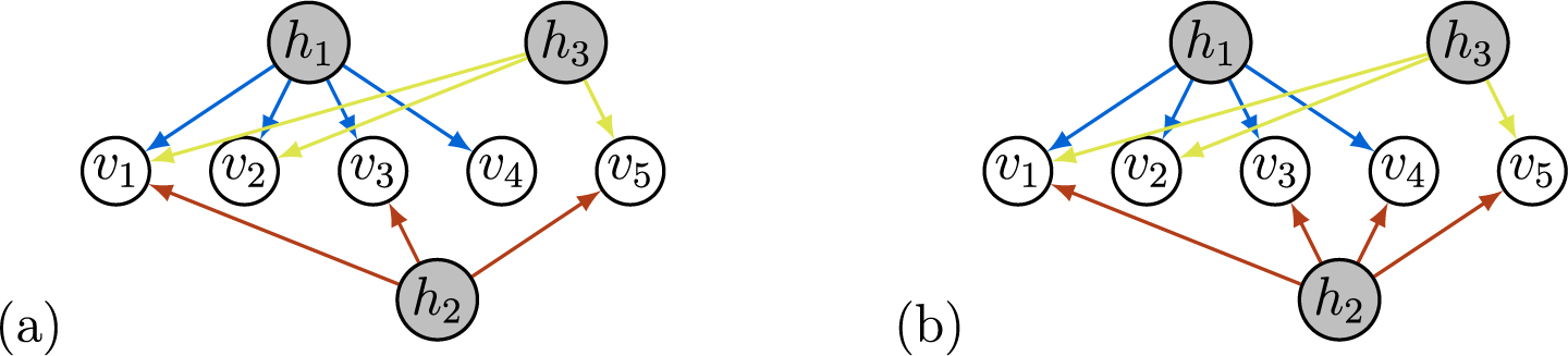
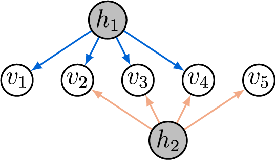
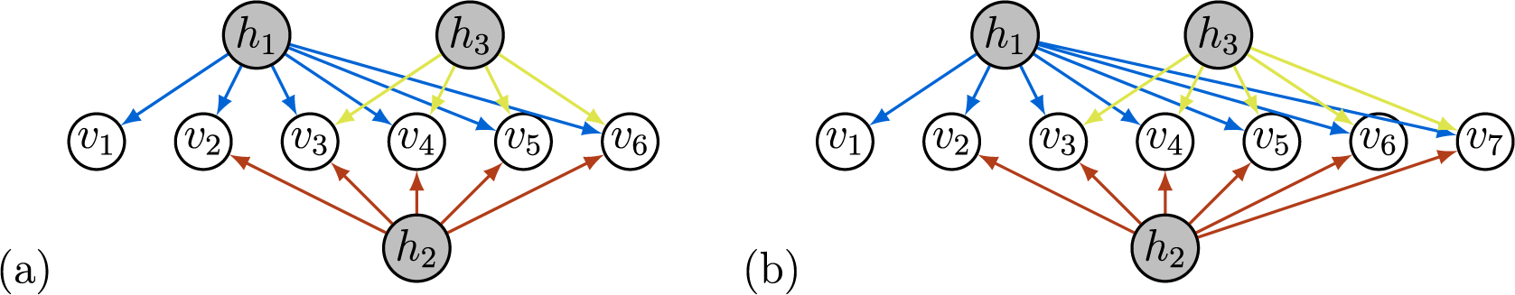
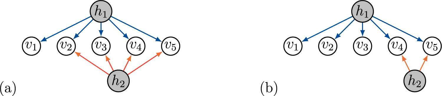
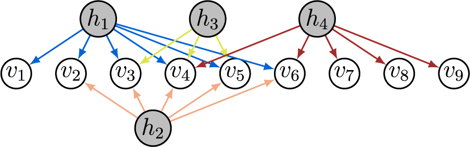
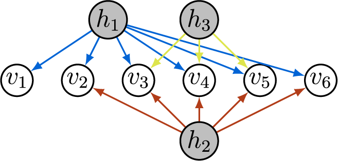
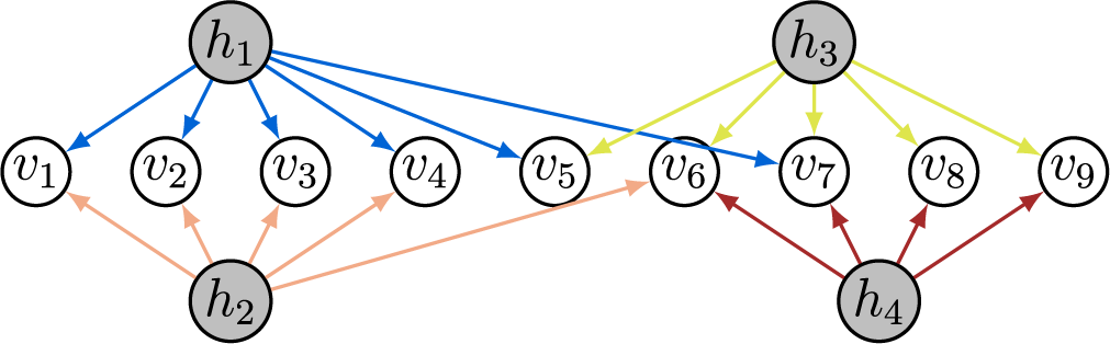
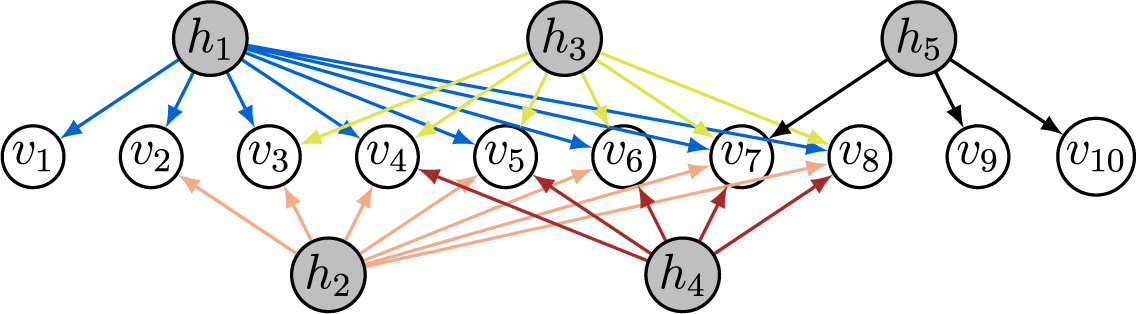
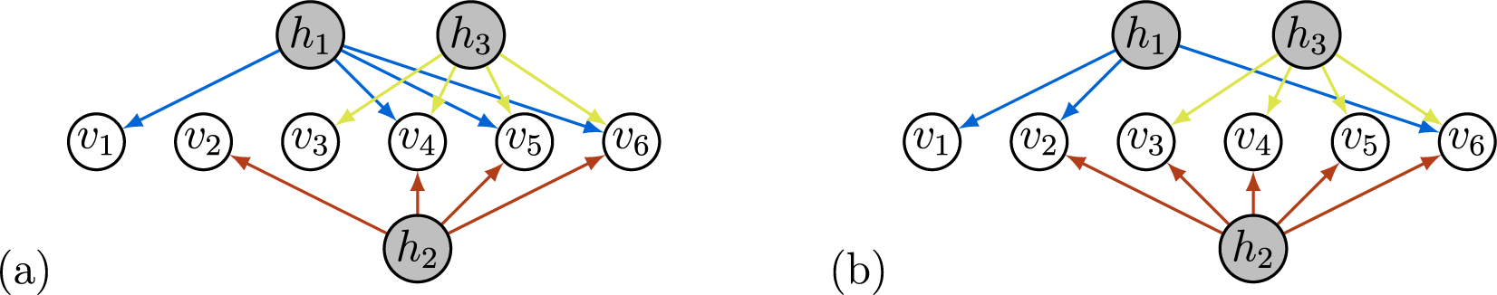
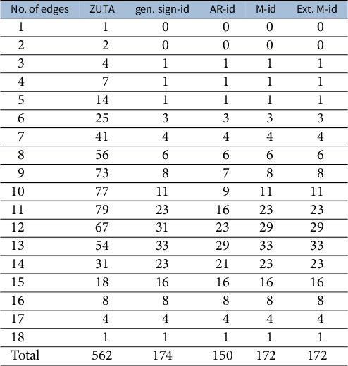


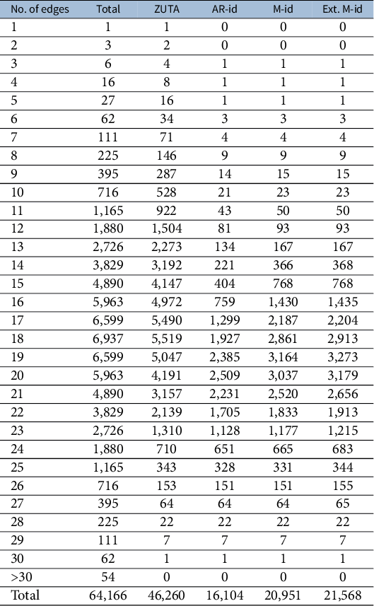


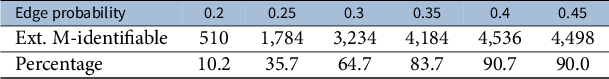


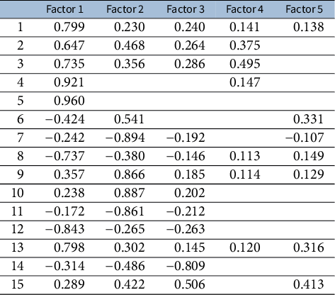
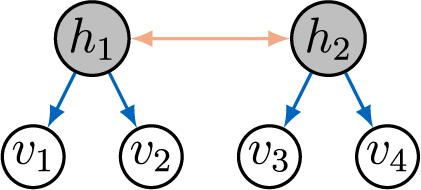


 Open access