

1. Introduction
The sensitivity of glaciers to local climate change makes them an obvious and widely used indicator of global climate change (Reference VaughanVaughan and others, 2013). Global warming during recent decades has had significant impacts on the world’s glaciers, which have experienced intensified ice mass loss induced by strengthened ablation, and thus thinning (e.g. Reference Rivera, Benham, Casassa, Bamber and DowdeswellRivera and others, 2007; Reference James, Murray, Barrand, Sykes, Fox and KingJames and others, 2012; Reference Lee, Shum, Tseng, Huang and SohnLee and others, 2013; Reference Racoviteanu, Arnaud, Williams and ManleyRacoviteanu and others, 2014), along with universal retreat and shrinkage (e.g. Reference Granshaw and FountainGranshaw and Fountain, 2006; Reference Bown, Rivera and AcunaBown and others, 2008; Reference Mehta, Dobhal, Pratap, Verma, Kumar and SrivastavaMehta and others, 2013). The special location of the Tibetan Plateau and surrounding mountains in global circulation systems, along with the huge topographic landforms, has resulted in extensive glacier coverage in western China (Reference YaoYao and others, 2012). Under the influence of rapid climate change in Chinese territory (temperature increase 0.23°C (10 a)–1 during 1951–2009; Reference QinQin, 2012), glaciers in China have experienced dramatic changes (e.g. Reference Shangguan, Liu, Ding, Ding, Xu and JingShangguan and others, 2009; Reference BolchBolch and others, 2010b; Reference PanPan and others, 2012; Reference WangWang and others, 2014). However, understanding the influences of Chinese glacier changes on regional environments is dependent on comprehensive information about total glacier coverage in China, which can only be revealed by glacier inventory work.
In 1978, a group of Chinese scientists started to compile the first Chinese glacier inventory (CGI-1) under the leadership of Yafeng Shi. This work was finished in 2002, and resulted in 12 volumes and 21 glacier inventory books (Reference Shi, Liu, Ye, Liu and WangShi and others, 2008, Reference Shi, Liu and Kang2009). According to CGI-1, there were a total of 46 377 glaciers in China, covering 59 425 km2, with an estimated total ice volume of ∼5600 km3. These account for 23% of the number and 8% of the area of global glaciers in the Randolph Glacier Inventory (RGI, version 3.2; 197 654 glaciers with a total area of 726 792 km2), and half of the glacier area in regions surrounding the Tibetan Plateau (RGI regions 13–15; total area 118 264 km2) (Reference PfefferPfeffer and others, 2014). A concise version of CGI-1 was presented by Reference Shi, Liu, Ye, Liu and WangShi and others (2008).
CGI-1 was compiled based on topographic maps and aerial photographs acquired during the 1950s–80s. Its historical time span cannot represent the contemporary glacier status in China. In 2006, the Ministry of Science and Technology of China (MOST) launched a project entitled ‘Investigation of Glacier Resources and their Changes in Western China’, which aimed at the compilation of most parts of the second Chinese glacier inventory (CGI-2), and the digitization of CGI-1 based on the scanned copy of topographic maps used during its compilation (Xu and others, in press). The compilation of CGI-2 was based on remote-sensing and GIS techniques, with some in situ field investigations to provide validations and detailed monitoring of selected glacier changes. The currently compiled CGI-2 has a total area of 43 087 km2 up until 2013, and covers 86% of the glacierized area of China relative to the digitized CGI-1 (DCGI-1). The remaining regions are mainly located on the southeastern Tibetan Plateau, which is dominated by the Indian monsoon and nearly permanently covered by seasonal snow and cloud, so good-quality optical satellite images can rarely be acquired.
Here we provide a brief introduction to the data and methods used to compile CGI-2, and evaluate uncertainties in glacier delineations and corresponding glacier area accuracy. We also summarize glacier distribution characteristics. Some important issues in remote-sensing based compilation of glacier inventories, including the critical challenges faced by the simple band ratio segmentation method and methods of evaluating glacier area accuracy, are discussed.
2. Drainage Basins and the Coding System in Western China
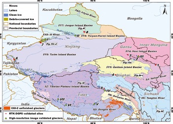
The Temporary Technical Secretariat of the World Glacier Inventory (TTS/WGI) designed a coding system to identify glaciers (Reference Müller, Caflisch and MüllerMüller and others, 1977). According to this, the glacier identifier is composed of identifiers of country (up to three characters), continent (one character), drainage basin (four characters) and the glacier sequence number (three characters). CGI-1 followed this convention but modified it slightly (Reference Shi, Liu, Ye, Liu and WangShi and others, 2008). The country code of China (CN) and the continent code of Asia (5) were assigned to all drainage basins as the first three characters. Then all glacierized regions in China were divided into 10 first-order, 30 second-order, 103 third-order, 349 fourth-order and 1430 fifth-order drainage basins. The glacier sequence number was also assigned four characters because some fifth-order basins have >999 glaciers. In CGI-2, the glacier identifier uses the GLIMS (Global Land Ice Measurements from Space) ID system with the form of GnnnnnnEmmmmm [N|S], where n and m are longitude and latitude (in millidegrees) of glacier label points (Reference Raup and KhalsaRaup and Khalsa, 2010). However, the drainage basin information from the WGI glacier identification system was retained in CGI-2 to indicate to which drainage basin the glacier belongs. The first-order (second-order for 5A, 5X and 5Y) drainage basins in western China and their identifiers are shown in Figure 1.
3. Data Used in Glacier Inventory Compilation
3.1. Landsat images
The remote-sensing based delineation of glaciers, especially by automatic methods, is mostly dependent on the presence of a shortwave infrared band in the satellite sensor, which can capture snow and ice signals with distinctive lower reflectance compared to other land surfaces (Reference O’Brien, Munis and RangoO’Brien and Munis, 1975; Reference WarrenWarren, 1982). The accommodation of such bands and the moderate resolution characteristics of Thematic Mapper (TM) and Enhanced TM Plus (ETM+) sensors on board the Landsat series satellites, plus open access to the acquired images after 2008 (Reference WoodcockWoodcock and others, 2008) and the higher orthorectification accuracy of the images provided by the US Geological Survey (USGS) (http://earthexplorer.usgs.gov/; Reference Bolch, Menounos and WheateBolch and others, 2010a; Reference Guo, Liu, Wei and BaoGuo and others, 2013; Reference Livingstone, Clark, Woodward and KingslakeLivingstone and others, 2013), have made them the most popular source for glacier inventory compilation (e.g. Reference Aniya, Sato, Naruse, Skvarca and CasassaAniya and others, 1996; Reference Sidjak and WheateSidjak and Wheate, 1999; Reference Narama, Shimamura, Nakayama and AbdrakhmatovNarama and others, 2006; Reference Paul, Andreassen and WinsvoldPaul and others, 2011a; Reference Rastner, Bolch, Mölg, Machguth, Le Bris and PaulRastner and others, 2012). The CGI-2 also adopts the Landsat series images to delineate glaciers.
Figure 2a and b show the temporal distribution of Landsat scenes used in CGI-2. In total, 126 Landsat scenes are needed to cover the glacierized regions of China. However, persistent snow and cloud cover in some regions made it difficult to delineate glaciers from a single Landsat image, so auxiliary images were needed. This led to the use of a total of 218 Landsat scenes in CGI-2. The scan line corrector (SLC) failure of ETM+ in 2003 seriously reduced image usability, and the ETM+ images were mostly used as auxiliary data. Most of the images used (∼89%) were acquired by TM. The time span of the images was 2004–11, with ∼63% of them being taken in 2007 and 2009 and ∼92% during 2006–10. By area, the proportions of glaciers delineated are 23% in 2007, 32% in 2009 and 26% in 2010. The absence of TM images in 2008 was due to the lack of Chinese territorial data on USGS websites (http://earthexplorer.usgs.gov/).
Spatio-temporal characteristics and qualities of Landsat scenes used, and dates of glaciers in CGI-2.
Glaciers in China are divided into those of continental type, whose greatest accumulation occurs during winter, and those of maritime type with strong summer accumulation (Reference Shi and LiShi and Li, 1981; Reference HuangHuang, 1990). The maritime glaciers are mainly distributed in the southern and eastern Tibetan Plateau, and commonly have extensive snow and cloud cover during their ablation seasons. This leads to seasonal dispersion in the distribution of images, some of which (14%) were taken during winter (November to March). However, most images were acquired during ablation seasons (April to October proportion is 86%), with ∼68% of scenes acquired around the end of ablation seasons (July to September), while the real glacier acquisition season is concentrated in August (30% of total area) and September (38%) (see Fig. 2b).
The accuracy of glacier delineation is mostly determined by seasonal snow around the glacier or within the debris-covered area, and by cloud cover over the glacier surface. To give an overview of the quality of Landsat images used, we use a value of 2.0 as the threshold for TM3/TM5 to differentiate snow within a five-pixel buffer of the glacier outline and debris-covered area (>2.0), and cloud within the clean-ice area (<2.0). The ratio of snow- and cloud-covered area to the total area of all glaciers and their buffers within the image was regarded as the proxy of image quality. The results show that 86% of images have <20% snow/cloud coverage, while ∼48% of images have <10% (Fig. 2c). All the selected ETM+ images have <20% cloud/snow coverage. The spatial distribution of image quality (Fig. 2d and e) shows that the lower-quality images (snow/cloud coverage >20%) are mainly concentrated in the western Himalaya region (30–32° N, 77–81° E) and Kunlun mountains (36° N), whereas the inland Tibetan Plateau (33–35° N, 84–90°E) has the best image quality.
3.2. Digital elevation models
Two kinds of digital elevation models (DEMs) were used during compilation of CGI-2. Delineations of the ice divide were based on DEMs (cell size 30 m) generated from digitized topographic maps, 1152 of which were 1 : 50 000 scale and 348 of which were 1 : 100 000, which were mainly constructed from aerial photographs acquired during the 1950s–80s. A rigorous seven-coefficient transformation was performed on the digitized contours and elevation points before DEM generation, to minimize potential errors introduced by mismatch of different coordinate systems between Landsat images and topographic maps, where the coefficients were calculated from coordinates of national trigonometric stations within and around those maps collected from the National Administration of Surveying, Mapping and Geoinformation of China. The Shuttle Radar Topography Mission (SRTM) DEM from the Consultative Group for International Agriculture Research (CGIAR), version 4, where voids were filled using different auxiliary DEMs (http://srtm.csi.cgiar.org), was used to derive glacier topographic attributes. The reasons for such DEM choices are described in Sections 4.2 and 7.3.
4. Methods of Compiling Glacier Inventory
4.1. Glacier delineation
Band ratio segmentation is the most robust and effective method of glacier classification (e.g. Reference PaulPaul, 2001; Reference PaulPaul and others, 2009; Reference Racoviteanu, Paul, Raup, Khalsa and ArmstrongRacoviteanu and others, 2009). During compilation of CGI-2, this method was adopted as a first step to delineate glaciers. Manual improvements after automatic delineation are considered essential, especially in the case of lower image quality (e.g. Reference Racoviteanu, Paul, Raup, Khalsa and ArmstrongRacoviteanu and others, 2009; Paul and others, in press). The lower image quality in many regions of western China required a great deal of manual work to improve the accuracy of glacier delineation, resulting in several rounds of manual improvements during compilation of CGI-2. The manual improvements were accomplished in the ArcMap workbench of the widely used ArcGIS software. In total, 12 participants were asked to take part in this work after in-depth training sessions on the pixel-mixing mechanisms and correct glacier discrimination from Landsat images of varying quality. However, the final check and improvements were performed by only five participants, who were constantly involved for >3 years in compiling CGI-2 and were experienced in glacier delineation. The excellent three-dimensional rendering of Google Earth™, along with its high-resolution images, can greatly facilitate discrimination of glacier ice from seasonal snow, cast shadow and, especially, debris-covered ice from surrounding moraines. During manual improvements, Google Earth™ image references via a plug-in of ArcMap (Export to KML) were found essential.
Several algorithms to automatically delineate debris-covered glaciers have been tested (e.g. Reference Taschner and RanziTaschner and Ranzi, 2002; Reference Paul, Huggel and KaabPaul and others, 2004; Reference Bolch, Buchroithner and KunertBolch and others, 2007; Reference Shukla, Arora and GuptaShukla and others, 2010). However, the low accuracy of their results obstructs their wider application, and it is recommended that they be used only as starting points for manual delineations (Reference PaulPaul and others, 2009, in press). Thus, delineation of debris-covered ice in CGI-2 was entirely based on manual digitization, as in most earlier studies (Reference Hall, Williams and BayrHall and others, 1992; Reference Racoviteanu, Arnaud, Williams and OrdonezRacoviteanu and others, 2008, Reference Burns and NolinBurns and Nolin, 2014). Manual digitization of debris-covered glaciers was mainly based on the recognition of distinctive surface features such as supraglacial lakes, the outlets of subglacial streams near glacier termini, and the landforms and drainage systems of lateral moraine, relying on the difference of surface colours and textures in different red, green, blue composites of Landsat images. The proper discrimination of debris-covered glaciers depended on the above features and was an important theme during the training of inventory participants.
4.2. Extraction of ice divides
The delineation of ice divides is vitally important in glacier inventory compilation (Reference Kienholz, Hock and ArendtKienholz and others, 2013). All widely used methods to delineate ice divides are based on the availability of DEMs and hydrological modeling tools. These methods can accurately split the glacier complex into individual glaciers if high-resolution DEMs are used. However, determination of the ‘pour point’ (the pixel toward which all water in a basin flows) of each individual glacier drainage basin in these methods can mostly only be done by visual inspection, involving large workloads. Reference Kienholz, Hock and ArendtKienholz and others (2013) have now developed a new method to automatically determine the pour point of each glacier basin and merge watersheds belonging to the same glacier.
All previous methods, including that developed by Reference Kienholz, Hock and ArendtKienholz and others (2013), can be called bottom-up methods, and mainly focus on the determination of outlet points of glacier drainage basins below the glacier termini. In CGI-2, we developed a ‘top-down’ method, which ignores the downstream problems and only considers actual ice divides. A set of Interactive Data Language (IDL) procedures was developed to do this work. The input data were prepared by hydrological analysis tools in the ArcInfo Workstation. They were executed by an Arc Macro Language (AML) script in IDL, and further processes were also implemented with IDL programming. Figure 3 shows the main workflow of this top-down method. The drainage basin boundaries were extracted using recoded streamline segments as their pour points. The ice divides were identified by aspect differences between the two sides of mountain ridges. Larger aspect difference denotes real ice divides, while smaller difference indicates artifacts or interferences, which are discarded. Several parameters need to be predefined (annotations on lines in Fig. 3) including two that are important: the minimum drainage basin area and minimum aspect difference. These were chosen differently in different regions.
Flow chart to extract ice divides from a DEM. The left part was done with ArcInfo Workstation (command line module of ArcGIS) using integrated AML scripts, and the right part was done with IDL procedures developed by the authors.
Figure 4 shows some examples of ice-divide extraction by the top-down method. Although some manual work is still needed after automatic extraction, it is a simpler process which mainly focuses on deleting residual spurious ice divides resulting from complex terrain within the glacier. Different DEMs give different results. DEMs generated from 1 : 50 000 topographic maps give the best results with sufficient details, and thus were selected to extract ice divides in CGI-2. The artifacts of Advanced Spaceborne Thermal Emission and Reflection Radiometer (ASTER) Global DEM (GDEM) version 2 on steep terrain and areas above the accumulation regions of glaciers led to the worst results (Fig. 4b).
Ice divides in Anyemaqen mountains, Qinghai Province, extracted from (a) SRTM, (b) GDEM2 and (c) 1 : 50 000 topo-DEM. The intersected and modified ice divides in (c) are shown in (a) and (b) for comparison. The other examples are ice divides extracted from 1 : 50 000 topo-DEMs for (d) Gongga mountains, Sichuan Province, (e) Purogangri, Tibet Province, and (f) Bogda mountains, Xinjiang Province. MBA and MAD are the minimum basin area and minimum aspect difference, respectively.

4.3. Attributes for individual glaciers
According to the old guidelines of WGI (UNESCO/IASH, 1970; Reference Müller, Caflisch and MüllerMüller and others, 1977), many attributes of a glacier need to be assigned in the glacier inventory, including glacier name, drainage basin ID, source material, area, width, length, elevation, classification, etc. In remote-sensing- and GIS-based compilation of glacier inventories, some of these attributes still require much manual processing and glaciological expertise, so the latest guidelines for remote-sensing-based glacier inventories (Reference PaulPaul and others, 2010) recommend delayed assignment of several attributes such as glacier name, WGI code, clean-ice area, classification, etc., for quick compilation of glacier inventories in the GLIMS framework.
In CGI-2, we assigned most attributes recommended by Reference PaulPaul and others (2010) except glacier length. Some researchers have developed several algorithms to automatically extract glacier center lines for glacier length calculation (e.g. Reference Le Bris and PaulLe Bris and Paul, 2013; Reference Kienholz, Rich, Arendt and HockKienholz and others, 2014; Reference Machguth and HussMachguth and Huss, 2014). However, the automatically extracted glacier center lines also require manual improvements. The large number of glaciers in China makes such work time-consuming, so currently the glacier length has not been assigned.
Most of the assigned attributes were calculated using methods similar to those suggested by Reference PaulPaul and others (2010). The glacier areas were calculated in an Albers equal-area conic projection with standard parallels at 25° N and 47° N. The label points of glacier polygons were generated automatically in ArcInfo Workstation (procedure CreateLabels) and checked by visual inspection one by one. Points close to the glacier outline were relocated to better represent the glacier location. The source image attribute was divided into two fields, i.e. the primary image and the auxiliary image, while the representative date of the glacier was only derived from the primary source.
As mentioned in Section 3.1, the topographic attributes were calculated based on SRTM version 4. To avoid inaccurate cell exclusion and inclusion when masking the DEM with the glacier outline, the SRTM DEM was resampled into the same resolution as TM (30 m) using the bilinear interpolation method. The maximum, minimum and mean elevations were then extracted from statistics of all resampled SRTM DEM cells located within the glacier outline, while the median elevation was extracted as the 50th percentile of the cumulative number distribution of cell elevations. The mean slope was simply determined by the average value of slope across all cells. The mean aspect was calculated by dividing the mean sine by the mean cosine of aspect across all cells (Reference PaulPaul and others, 2010).
5. Error Assessments
5.1. Methodological accuracy of glacier delineation
GLIMS has conducted several experiments to reveal the uncertainties in glacier inventory compilation using different methods (GLACE 1 and GLACE 2; Reference RaupRaup and others, 2007). The sources of glacier delineation errors can be divided into three classes (Reference RaupRaup and others, 2007; Reference Paul and AndreassenPaul and Andreassen, 2009): technical errors, interpretation errors and methodological errors. Technical errors can be mostly ignored if the satellite image has been accurately orthorectified, which was the case for Landsat images provided by USGS (e.g. Reference Bolch, Menounos and WheateBolch and others, 2010a; Reference Guo, Liu, Wei and BaoGuo and others, 2013). Interpretation errors mostly depend on how ‘glacier’ is defined for the purposes of inventory compilation, and thus are difficult to evaluate. Methodological errors were largely decided by the resolution of the Landsat images, and the skills of the inventory compilers which also cannot accurately be assessed (Reference PfefferPfeffer and others, 2014). In the case of CGI-2, the GLIMS guidelines (Reference Racoviteanu, Paul, Raup, Khalsa and ArmstrongRacoviteanu and others, 2009; Reference PaulPaul and others, 2010) were followed to minimize interpretation error, and the compilers were well trained to enhance their skills. However, the glacier mapping error still needs to be properly evaluated. This was done by incorporating all error sources into one term, i.e. methodological errors, which were determined by comparing the glacier outlines with the glacier marginal positions measured during field GPS investigation, and the glacier outlines delineated from high-resolution Google Maps™ images.
Many real-time kinematic differential GPS (RTK-DGPS) measurements (Unistrong E650 GPS instruments) were obtained during field investigations in 2007–08 (Reference Shangguan, Liu, Ding, Zhang, Du and WuShangguan and others, 2008, Reference Shangguan, Liu, Ding, Zhang, Li and Wu2010; Reference Li, Liu, Shangguan and ZhangLi and others, 2010), which also included many measurements of glacier boundaries. These measurements have very high accuracy (±10.1 to ±10.3 m) compared to the coarse spatial resolution of Landsat images used in CGI-2. However, the GPS measurement dates mostly differ from the acquisition dates of the best images selected to compile the glacier inventory in these regions. We use the GPS measurements to evaluate the positioning accuracy of glacier outlines delineated from Landsat images with dates as close as possible to the GPS measurement dates. The same delineation methods were used as in compiling CGI-2 (see Fig. 5 for examples). Other errors (e.g. mis-registration of Landsat images or incorrect recognition of boundaries of debris-covered glaciers during field investigation) may also be significant, but our GPS–Landsat comparisons give an overview of the methodological accuracy in glacier inventory compilation.
Examples of glacier outline accuracy assessments by field RTK-DGPS measurements: (a) central Qilian mountains (RC1 in Fig. 1 and Table 1; glaciers No. 1 and No. 5 in Shuiguan river basin); (b) western Qilian mountains (RC3; Laohugou glacier No. 12); and (c) central Tien Shan (RC8; Fenliu glacier, Bogda peak).
In total, 23 glaciers (see Fig. 1 for the distribution of measured glaciers) were measured by RTK-DGPS, with >2320 measurements located on the glacier margins (Table 1). Landsat images of acceptable quality and with similar acquisition dates to the GPS measurements (maximum difference ∼1 year) were downloaded from the USGS website.
Offsets (m) between field GPS measurements and glacier outlines delineated by the methods of CGI-2. RC is region code, M-Date is date of GPS measurements, A-Date is date of Landsat image acquisition, NG is number of surveyed glaciers, NP is number of measured boundary GPS points, STD is standard deviation, and the prefixes A- and M- indicate automatically extracted and manually improved glacier outlines, respectively
Table 1 shows the results of comparisons between GPS measurements and delineated glacier outlines. The accuracy is ∼±18 m for automatically delineated and ∼±11 m for manually improved glacier outlines, while the accuracy of manually delineated outlines of debris-covered ice is in the order of ±30 m.
In addition to the field RTK-DGPS measurements, we used high-resolution satellite images to validate the accuracy of the glacier delineation methods in CGI-2 (see Fig. 6 for a typical case), as in previous studies (Reference PaulPaul and others, 2013). The high-resolution screenshots of Google Maps™ were captured for seven randomly selected regions (see Fig. 1 for their distribution), where higher-resolution images in Google Maps™ and nearly simultaneous Landsat images are available. Only images with a spatial resolution better than 1 m in Google Maps™ were selected. The glacier outlines on the screenshots of Google Maps™ were manually digitized and regarded as the ground truth. They were then compared with automatically extracted and manually improved glacier outlines from nearly simultaneous Landsat images. The debris-covered glaciers were also manually digitized from both kinds of images. The offsets between Landsat and Google Maps™ outlines were calculated as the distances between points taken every 10 m along the Landsat outline and the nearest points on the corresponding Google Maps™ outline. The glacier area differences between the two sets of results were also calculated (Table 2).
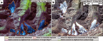
Offsets (m) of glacier outlines that were automatically delineated and manually improved from Landsat images compared with outlines manually digitized from high-resolution screenshots of Google Maps™. RC is region code, H-Date is acquisition date of Google Maps™ images and L-Date is date of Landsat images
The results of high-resolution image validation in Table 2 give offsets similar to those in Table 1. The average offsets also suggest better accuracy after manual improvement (11.37 m vs 17.03 m). The uncertainties in debris-covered glacier outline delineation are still high in this validation, illustrating the difficulties of accurate delineation of debris-covered glacier outlines.
5.2. Glacier area error assessment
The glacier area error tends to be inversely proportional to the length of the glacier margin (Reference PfefferPfeffer and others, 2014), so it depends strongly on the size of the glacier (larger glaciers mostly have longer margins). In this sense, the area error assessed by glacier buffers (Reference Granshaw and FountainGranshaw and Fountain, 2006; Reference Bolch, Menounos and WheateBolch and others, 2010a) is rational because it accounts for the length of the glacier perimeter. The buffer width, however, is critical to the resultant glacier area error.
The area error assessment of CGI-2 uses a method similar to the buffer method suggested by Reference Rivera, Bown, Casassa, Acuna and ClaveroRivera and others (2005), and includes both the length of glacier outlines and their positioning accuracies. The above assessments of methodological accuracy suggest ∼±10 m and ∼±30 m for clean-ice and debris-covered glacier outline delineation, respectively. Regarding the mis-recognition of glacier boundaries in the field and mis-registration of satellite images, as well as the influence of seasonal snow remnants, we consider the ±10 m and ±30 m accuracies for clean-ice and debris-covered glacier outlines as a reasonable basis for evaluating their area error. The boundaries between clean-ice and debris-covered ice were mostly not manually improved, so their positioning accuracy was regarded as ±15 m, a value used by some researchers (e.g. Reference Bolch, Menounos and WheateBolch and others, 2010a; Reference Rastner, Bolch, Mölg, Machguth, Le Bris and PaulRastner and others, 2012). As described in Section 4.2, the delineation of ice divides is vitally dependent on the DEM used, so their accuracy is difficult to evaluate. In CGI-2, we used the DEM pixel size (30 m for 1 :50 000 topo-DEM used in CGI-2) as the positioning accuracy of ice divides in area error calculations. The area error evaluations in CGI-2 were then calculated using
where EA
is the glacier area error, L
c, L
d and L
i are the length of clean-ice, debris-covered glacier outlines and ice divides, respectively, and ![]() ,
, ![]() and
and ![]() are their positioning accuracies.
are their positioning accuracies.
Equation (1) was used in area error calculations for every individual glacier. The errors at boundaries between clean and debris-covered ice make no contribution to the error of the whole glacier area. At drainage-basin and larger scales, the errors at interior ice divides are also omitted. The resulting glacier area errors of the 15 basins and the whole of CGI-2 are shown in Table 3. The area error of all compiled glaciers in CGI-2 was ±3.2%. The largest area error was ±8.6% in the Keboduo river basin (5Y124), which only has 0.8 km2 of glaciers. The errors of debris-covered areas were much larger than those of whole glacier areas, amounting to ±17.6% for all debris-covered ice in CGI-2.
Glacier distributions in different drainage basins of western China from CGI-2, and their comparisons to CGI-1 and DCGI-1. R. indicates river, and I.B. inland basins
6. Results
6.1. General results of CGI-2
In total, 42 370 glaciers were compiled in the current CGI-2, with a total area of ∼43 087 km2 (Table 3). The minimum area of glaciers compiled is 0.01 km2. About 59% of the compiled glaciers are distributed in the Ganges river basin and Tarim inland basin, and 16% are distributed in Tibetan Plateau inland basins. The current compiled glaciers in CGI-2 correspond to a total area of ∼52 043 km2 of glaciers in DCGI-1 (∼86% of the total). Approximately 90% of the area (7840 km2 from DCGI-1) of uncompiled glaciers is located in the Ganges river basin, while 9% and 1% are in the Yangtze and Salween river basins, respectively.
A general feature of glacier size distributions is that large numbers of small glaciers account for a small proportion of total area, and a lesser number of larger glaciers account for most of the total area (Reference Paul and SvobodaPaul and Svoboda, 2009; Reference Le Bris, Paul, Frey and BolchLe Bris and others, 2011; Reference Bliss, Hock and CogleyBliss and others, 2013; Reference Hagg, Mayer, Lambrecht, Kriegel and AzizovHagg and others, 2013). This feature is also very clear in China. The distribution of glaciers of different sizes is shown in Figure 7. Most glaciers (∼83% of the total) have an area of <1 km2 (Fig. 7c), and only ∼3% of glaciers have an area larger than 5 km2. However, the total area occupied by glaciers smaller than 1 km2 only amounts to 20% of the total CGI-2 area (Fig. 7d), while glaciers larger than 5 km2 occupied 51% of the area.
Total glacier numbers (a) and area (b) of CGI-2 and their respective proportions (c, d) within different area classes and different drainage basins.
The distribution of glaciers within different area classes in different drainage basins (Fig. 7c) exhibits similar patterns to Table 3. However, the number and area of glaciers of each area class are different in each drainage basin. The number proportion of glaciers smaller than 1 km2 is close to 80% in most drainage basins, but is very high (∼90%) in the Salween river (5N), Indus river (5Q) and Turpan–Hami inland basins (5Y8), which means that these three drainage basins have more small glaciers. Glaciers larger than 5 km2 are concentrated in the Ganges river (5O), Tarim basin (5Y6) and Tibetan Plateau inland basins (5Z) (amounting to 17%, 47% and 19% of the total area of >5 km2 glaciers in CGI-2, respectively). Glaciers larger than 50 km2 are also concentrated in these three drainage basins (amounting to 97% of the total area of all >50 km2 glaciers), while all glaciers larger than 100 km2 are located within these basins, including the largest glacier in CGI-2, Insukati glacier (359 km2) in Tarim basin. On the other hand, the larger area proportions of glaciers smaller than 1 km2 in the Salween river (5N), Indus river (5Q), Turpan-Hami inland basins (5Y8), Mekong river (5L), Hexi (5Y4) and Junggar inland basins (5Y7) indicate that more glaciers in these six basins are small glaciers. The lower area proportions of >5 km2 glaciers in these six basins also illustrate the dominance of small glaciers.
6.2. Glacier hypsography
Glacier hypsography can provide useful information for understanding the regional topography, geomorphology and climate (Reference MeierMeier and others, 2007). Figure 8b shows the glacier hypsography with 100 m elevation intervals of 14 larger mountain systems in western China (Fig. 8a). About 57% of the glacier area is distributed in the 5000–6000m elevation range, while 26% is located below 5000 m, and only 17% above 6000 m.
Mountain systems defined in CGI-2 (a) and their glacier hypsography (100m elevation interval) (b). Gray lines in (b) are the median elevations of all inventoried glaciers in corresponding mountain regions. Note that in (b) the scale on the horizontal axis differs from region to region.

For the elevation of maximum glacier area distribution, an overall south-to-north trend of slight increase followed by sharp decrease can be identified from Figure 8b. The highest modal elevation (most heavily glacierized) appears in the Gangdise mountain range (∼5900 m). The modal elevation shows a slight increase from the Himalaya range (∼5800 m) to the Gangdise range. Then it retains this level of ∼5900 m to the Qiangtang plateau, Karakoram mountain range and Kunlun range, and decreases sharply northwards from the Tien Shan and the Saur range to the Altai. The Altai mountains have the lowest glaciers in China (minimum elevation 2360 m).
Two overall west-to-east descending trends of the modal elevation can also be identified from Figure 8b. The first descending trend is located along the southern Tibetan Plateau, where the modal elevations decrease from the Gangdise range to the Nyenchen Tanglha mountain range (∼5830 m) and then to the Hengduan mountain range (∼5440 m). Another west-to-east descending trend is located along the northern edge of the Tibetan Plateau, where the highest modal elevation is ∼5890 m at the Kunlun, descending to ∼5290 m at the Altun and then to ∼4980 m at the Qilian. The bimodal glacier hypsography of the Kunlun mountains is explained by the concentrations of three large glacier centers. The first center, located on the west Kunlun mountain range, has a mean elevation >5800 m, and the glacier area occupies nearly one-tenth of CGI-2. The other two centers, namely Muztag peak (aka Muztagh Ata) and Xinqing peak, are located within the central and eastern Kunlun mountain ranges, with ∼1300 km2 of glaciers and mean elevations of ∼5400 m.
6.3. Distribution of glaciers of different orientation
Figure 9 shows the glacier area distributions within different slope and aspect ranges in 14 mountain systems of western China and the whole of CGI-2, in which areas are calculated by counting the number of glacier DEM cells in different aspect and slope ranges rather than the mean slopes and aspects of all glaciers. The mean glacier surface slope of CGI-2 is 19.9°. The Pamir plateau, Qilian mountain range, and Altun mountains have the steepest glacier surfaces, where ∼two-thirds or more of the glacier areas have a surface slope greater than 15°. By contrast, Qiangtang plateau and the Tanglha mountains have the gentlest glacier surfaces, where more of the glacier areas are distributed below 15° (area proportions below 15° reaching 64% and 59%, respectively). The glacier area distribution within different aspect ranges also shows remarkable spatial discrepancies. An overall characteristic is the predominance of north-northeast-facing glaciers with a mean aspect of 24.3°. The proportions of north- (315–45°) and east-facing (45–135°) glacier areas are 39% and 28%, respectively. Glaciers in the Saur, Qilian, Altun and Gangdise mountains show very distinctive north-facing characteristics; the areal proportions of north-facing glaciers all exceed 50%. By contrast, glaciers in the Karakoram mountains, Qiangtang plateau and Hengduan mountains show the dominance of northeast facing, where the proportions of north- and east-facing glacier areas all exceed 30%.
Glacier area distribution within different surface slope (5° interval) and aspect (11.25° interval) ranges for 14 mountain systems in western China (Fig. 8a) and the whole of CGI-2. Black lines indicate the mean glacier surface slopes and aspects. The area values were obtained by counting pixels in each slope and aspect range, and the mean slope and aspect were also calculated from all glacier pixels in each mountain system.
Analysis of the orientation of different glacier sizes shows that smaller glaciers (<2 km2) are more likely to be located on north-facing slopes (area proportion 56%), while larger glaciers are more evenly distributed on north- and east-facing slopes (the area proportion of east-facing glaciers larger than 2 km2 amounts to one-third versus one-fifth of glaciers smaller than 2 km2). The glaciers larger than 5 km2 in the Tien Shan, Karakoram, Gangdise, Hengduan and Nyenchentanglha mountains and the Pamir and Qiangtang plateaus are mostly distributed on the east- rather than north-facing slopes. By contrast, most of the glacier area in the Kunlun, Qilian and Altun mountains tends to be distributed on north-facing slopes.
6.4. Distribution of debris-covered glaciers
In total, 1723 glaciers are covered by 1493.7 km2 of debris in CGI-2 (Table 3). The average ratio of debris-covered area to total glacier area for these glaciers is 12%. Glaciers with debris-covered area are mostly concentrated in five centers: Tumur peak, Tien Shan; eastern Pamir plateau; Karakoram; the Himalaya; and Gangrigabu peak, Nyenchen Tanglha mountains (see Fig. 1 for distribution of debris-covered glaciers). Tumur peak is the largest debris-covered glacier center. The area of debris-covered ice in this region amounts to 29% (430 km2) of the total area of debris-covered ice in CGI-2, and accounts for 14% of the total area of debris-covered glaciers in this region. The two largest debris-covered glaciers in China are located on Tumur peak. Tumur glacier, which has the largest debris-covered area in CGI-2, has a debris area of 63 km2 (∼17% of its total area), and the debris extends to 4520 m a.s.l. (∼two-fifths of the glacier’s elevation range, 2890–7030 m). The second-largest debris-covered glacier is Tugbelqi glacier, which has a debris area of 39 km2 (13% of its total area), and the highest elevation of debris is 4267m (also ∼two-fifths of the glacier’s elevation range).
The Himalaya and the eastern Pamir plateau are two other major centers of debris-covered glaciers. About 19% (283 km2) of debris-covered area is distributed in the Himalaya, of which ∼70% (199 km2) is distributed in regions around Qomolangma (Mount Everest), Lapche Kang and Shishapangma. The eastern Pamir plateau is the third-largest center of debris-covered glaciers, with a total debris-covered area of 207 km2 (14% of CGI-2). Most (∼65%; 134 km2) of the debris-covered area in this region is distributed on Kongur Tagh and Muztagh Ata.
7. Discussion
7.1. Glacier delineation
The band ratio segmentation method proved robust and efficient when the best-quality imagery was available. Our method experiments also revealed the insensitivity of the band ratio segmentation method to the band ratio thresholds when high-quality satellite imagery is used and on gentler terrain (Fig. 10a and b). The generally achievable discrimination of 0.1 on the band-ratio threshold in the range 1.0–3.0 will only result in an area difference of ∼0.1 km2 (100 km)–1. This will lead to an area error of ∼±10.3%, assuming a typical perimeter/area ratio of ∼3 km km–2 (the mean from CGI-1). However, as illustrated by Reference Racoviteanu, Paul, Raup, Khalsa and ArmstrongRacoviteanu and others (2009), the fully automatic glacier outline delineation using this method was often obstructed by numerous factors, especially when image quality was poor, and in regions with larger elevation differences where strongly ablating areas on glacier tongues commonly coexist with melting snow remnants close to or above the equilibrium line, or in areas with thin clouds or shadows (Fig. 10c and d). Such regions are very common in western China, and such confounding factors can usually only be resolved by manual digitization, requiring many hours of work. The absolute determination of a pixel as either glacier or non-glacier is another shortcoming of the band ratio segmentation method, which has been shown to underestimate the glacier area by excluding mixed pixels (Reference PaulPaul and others, 2013). This issue also arises when using other automatic classification methods.
The insensitivity of glacier area to band ratio threshold selection in case of high image quality and gentle terrain (a, b), and a typical case of problematic determination of optimal band ratio threshold to delineate glaciers with TM3/TM5 (c) and TM4/TM5 (d) when using lower-quality image and on rugged terrain. The sensitivity was tested within ±500 m buffers of glacier outlines (white loops in (a)) and by change in thresholds with steps of 0.05, 0.1 and 0.2 (b). White rectangles in (c) and (d) denote regions where different thresholds give contradictory results: (1) shadow, (2) thin cloud, (3) snow remnants and (4) glacier tongue. Date format is yyyy/m/dd.

In contrast to automatic glacier delineation methods, manual digitization can partly solve the problems induced by seasonal snow and can discriminate the ice in mixed pixels. However, Reference PaulPaul and others (2013) revealed larger uncertainties in manual glacier outline delineation. This study illustrated that the accuracy of manual work is vitally dependent on the experience of participants in correctly discriminating glacier and non-glacier pixels, and on their skill in identifying possible ice in mixed pixels along glacier outlines. Since the compilers of any one glacier inventory may vary greatly in their levels of experience and knowledge, manually improved or digitized glacier outlines by different participants can show very large differences (in order of 5–10%; Reference Paul, Andreassen and WinsvoldPaul and others, 2011a), even in repeated digitization by the same participants. However, the lower image quality in many regions of western China requires many hours of manual work. To minimize the errors induced by insufficient experience and knowledge of glacier delineation from multispectral satellite images, participants were intensively trained before their real work began, and only those who were constantly involved in glacier inventory compilation were selected for the final revision of the glacier outlines.
7.2. Error assessments
Direct evaluation of area errors by comparison with glaciers delineated from high-resolution images (Reference Paul, Andreassen and WinsvoldPaul and others, 2011a, Reference Paul2013) is likely to be affected by biases since the error is strongly size-dependent when expressed as a fraction of the total area. We used a more straightforward method to better evaluate the accuracies of manually improved glacier outlines, firstly assessing the positioning errors and then using them to evaluate the area errors. Some factors will also introduce uncertainties in the final glacier outline positioning errors, including: (1) discrepancies between validated outlines and real outlines of sampled glaciers in CGI-2, (2) mis-registration of satellite images, (3) incorrect recognition of glacier margins (especially margins of debris-covered ice) during fieldwork or on higher-resolution images, and (4) the preference for field GPS measurements in the ablation area. Of these factors, (2) and (3) will lead to overestimation of positioning errors, while (4) will result in underestimation. Furthermore, the selected validating points were aligned on both sides of referencing glacier outlines, in which different sides indicate different area errors (negative or positive). In this sense, the mean offsets of all points used in area error evaluation will result in overestimation. However, the selected ±10 m and ±30 m positioning error thresholds for clean ice and debris-covered ice were thought to be reasonable if counting all these factors together.
The substantial impacts of manual improvements on the positioning accuracy of automatically delineated glacier outlines demonstrated the need for such improvement (Reference RaupRaup and others, 2007). On the other hand, since no further co-registration was performed on either kind of satellite image used, the small offsets between the three kinds of glacier outline tend to confirm the acceptable orthorectification accuracy of Landsat images provided by USGS. This is also documented by previous studies (Reference Bolch, Menounos and WheateBolch and others, 2010a; Reference Guo, Liu, Wei and BaoGuo and others, 2013; Reference Livingstone, Clark, Woodward and KingslakeLivingstone and others, 2013).
In contrast to clean-ice outlines, our accuracy assessment for outlines of debris-covered ice faces more challenges. Although it is much easier to distinguish these outlines using high-resolution images, large uncertainties still exist because, no matter what the resolution of the image, debris-covered ice is difficult to discriminate from adjacent moraine or rock slopes. Even in the field, the margins of buried ice under debris covers are not always easily recognized (Reference Haeberli and EpifaniHaeberli and Epifani, 1986). However, since their validation is so difficult, the validations in this paper can provide valuable guidance on the accuracies we can achieve.
Besides glacier area errors, the assigned glacier attributes (e.g. maximum, minimum and median elevation, mean slope and aspect) must also contain some errors. However, these are more dependent on the accuracy and spatial resolution of the SRTM used. This accuracy could not be evaluated rigorously in the present study because of inconsistencies between the acquisition dates of the SRTM and Landsat images used, and also the lack of in situ measurements of glacier surface elevation.
7.3. DEM in CGI-2
Both SRTM and ASTER GDEM were considered for the extraction of glacier topographic attributes (Reference PaulPaul and others, 2010). However, although it has higher resolution, the existing undulations and artifact-related roughness variations in ASTER GDEM lead to very large differences (more than ±500 m; Reference Frey and PaulFrey and Paul, 2012), which can also be observed in Figure 4b. The broad range of acquisition dates due to the stacking of DEMs extracted from different ASTER scenes (Reference Fujisada, Urai and IwasakiFujisada and others, 2012) is another limitation of GDEM for topographic attribute calculations.
Although the data voids in steep terrain and underestimation of surface elevation in the accumulation area due to penetration of radar waves reduces its usability in glacier study, SRTM shows more uniform qualities within glacier-covered regions compared to ASTER GDEM, and has been used in the compilation of several glacier inventories (e.g. Reference BolchBolch and others, 2010b; Reference Le Bris, Paul, Frey and BolchLe Bris and others, 2011; Reference Paul, Frey and Le BrisPaul and others, 2011b) and glacier change studies (e.g. Reference Rignot, Rivera and CasassaRignot and others, 2003; Reference Aizen, Kuzmichenok, Surazakov and AizenAizen and others, 2006; Reference Bown, Rivera and AcunaBown and others, 2008). Reference Frey and PaulFrey and Paul (2012) found that SRTM is slightly better than GDEM in the compilation of topographic attributes of glacier inventories. Many other studies (e.g. Reference Zhao, Xue and LingZhao and others, 2010; Reference LiLi and others, 2013) have also illustrated the greater accuracy of SRTM than GDEM in Chinese territory. According to the above differences between SRTM and GDEM, the calculation of elevation attributes in CGI-2 employs SRTM as the main DEM source. The results shown in Figures 8 and 9 illustrate its good performance in such activities.
7.4. Comparisons between glacier inventories of China
CGI-1 has often been cited in previous research. Its submission to the GLIMS database further promoted its significance in scientific work, and it was included in the new RGI (Reference PfefferPfeffer and others, 2014). However, the glacier outlines compiled into the RGI were mostly digitized from 80 scanned digital copies of glacier inventory maps made during the compilation of CGI-1 (Reference Wu and LiWu and Li, 2004), which were concisely drawn from 1 : 50 000 and 1 : 100 000 topographic maps and have scales ranging from 1 : 100 000 to 1 : 1 000 000 (mostly 1 : 200 000 to 1 : 400 000). Furthermore, the glacier area in the original CGI-1 (total 59 425 km2; Reference Shi, Liu and KangShi and others, 2009) was entirely based on manual measurements by planimeter and thus affected by many artifacts. The data shown in Table 3 provided detailed information about the differences between the two versions of CGI-1. The glacier areas were underestimated by the original CGI-1 in most drainage basins, with a total underestimation of 1397 km2.
By detailed visual inspection, we found large differences between DCGI-1 and the current CGI-2, including the omission of some glaciers on topographic maps, larger differences in the acquisition dates of topographic maps used in CGI-1, different definitions of glaciers on steep terrain of accumulation areas, and the determination of debris-covered areas. The apparent glacier change in China (−17.2%) can be read from Table 3 by subtracting the corresponding CGI-1 area (52 043 km2) from the current CGI-2 area (43 087 km2), and this change rate can be considered even larger (∼17.9%) if we exclude CGI-2 glaciers omitted by CGI-1 (∼371 km2 total). However, such change analysis is not proposed since there are many differences between the DCGI-1 and current CGI-2. Furthermore, the image quality and glacier inventory accuracy of DCGI-1 will involve further work which is beyond the scope of this paper. Detailed change analysis will be introduced in a future paper.
7.5. About the unfinished part of the Chinese contemporary glacier inventory
The acquisition dates of Landsat images used to compile CGI-2 were originally planned to be confined to around 2008 to ensure the glacier inventory represented a nearisochronous assessment of the status of glaciers in China. However, the SLC failure of the Landsat ETM+ sensor in 2003, and the absence of TM images in 2008, significantly influenced Landsat image availability and expanded the range of acquisition dates. Nevertheless, 90% of our images are from 2006–10.
More than one-fifth of glaciers in China are distributed in the southeastern Tibetan Plateau. However, this region was almost permanently covered by snow and cloud due to the influence of the Indian monsoon. The available higher-quality images were all from beyond 2006–10. Some of the glaciers in this region (total area 2991 km2) were compiled using two TM scenes from 2005 which are of very good quality, but the glacier inventory in other parts of the region was deliberately not compiled, in order to preserve the temporal consistency of the new glacier inventory.
The Operational Land Imager (OLI) sensor on board Landsat-8 provides an excellent new mid-resolution image source to compile regional-scale glacier inventories and has the capability to acquire good-quality multispectral images. At the beginning of 2014, compilation of the glacier inventory in the southeastern Tibetan Plateau was resumed using images acquired by Landsat-8/OLI since 2013, and results are currently in manual checking and quality control. Because of the substantial date difference with the current CGI-2, the result is not presented in this paper and will be introduced in a future paper after the inventory has been completed.
8. Conclusions
The contemporary glacier inventory of China (CGI-2) was compiled based on 218 Landsat images (193 TM and 25 ETM+) acquired mainly during 2006–10. The widely used band ratio segmentation method was used as the first step in delineating glacier outlines, while intensive manual improvements were performed to improve accuracy and digitize debris-covered glacier areas. A self-developed top-down method, which mainly focuses on the actual topographic ridgelines rather than the determination of drainage basin outlets, was used to delineate ice divides based on DEMs generated from 1 : 50 000 and 1 : 100 000 topographic maps. The SRTM V4 was used to derive the topographic attributes of CGI-2.
Two methods were used to validate accuracies in CGI-2: field RTK-DGPS measurements on clean-ice and debris-covered glacier boundaries of 23 glaciers in different regions during 2007–08; and glacier outlines manually digitized from high-resolution images from screenshots of Google Maps™ in seven regions. The positioning accuracy of automatically and manually improved glacier outlines delineated from nearly simultaneous Landsat images was validated by these two references, and revealed that the accuracies for clean-ice and debris-covered glacier outlines are ∼±10 m and ∼±30 m, respectively. The ±10 mm and ±30 mm accuracies were then used to evaluate the glacier area errors, which resulted in ±13.2% area error for all glaciers (±17.6% for debris-covered glacier area) in CGI-2.
The results of the current compilation of CGI-2 include a glacier area of 43 087 km2 covering 86% of the glacierized regions of China. A total of 1723 glaciers in the current CGI-2 were debris-covered, with a total debris-covered area of 1493.7 km2. The unfinished parts of CGI-2 are mainly located in the southeastern Tibetan Plateau, where no Landsat scenes of acceptable quality can be found during 2006–10. They are still in the compilation process, with images acquired by Landsat-8 OLI after 2013
Acknowledgements
The compilation of CGI-2 was carefully supervised by the older generation of specialists who compiled the first glacier inventory of China, including Chaohai Liu, Zhen Su and, especially, Liangfu Ding who was untiringly involved in the whole inventory compilation process. We also thank the participants who spent so many hours and so much effort on this work. Special thanks are due to Ping Li, who devoted 5 years to the inventory compilation, and undertook the visual inspections and manual improvements for most of the glaciers in CGI-2. The CGI-2 compilation work was supported by funding from the National Foundational Scientific and Technological Work Programs of the Ministry of Science and Technology of China (grant Nos. 2006FY110200 and 2013FY111400) and Key Knowledge Innovation Programs of Chinese Academy of Sciences (grant Nos. KZCX2-YW-301 and KZCX2-YW-GJ04).


