


Impact Statement
The phenomenon of cricket ball swing is reviewed and reassessed using new results recorded for this paper. Swing bowling impacts the outcome of cricket matches; however, the existing scientific literature does not fully capture the behaviour recorded by ball tracking data in professional matches. This means that personal experience and anecdote still drive players, coaches, pundits and fans’ thinking around swing. Better understanding of the phenomenon will improve talent identification, coaching, selection, tactics and the wider public's enjoyment of the game.
The boundary layer aerodynamics responsible for swing are systematically described for varying Reynolds number, ball surface condition and free-stream turbulence to provide a comprehensive description of the physical mechanisms at play. Existing explanations are predominantly qualitative in nature, however, and the paper identifies further work needed to quantify realistic boundary conditions and their effect, and to analyse the problem within a statistical framework.
1. Introduction
The sport of cricket is a contest between two teams who are striving to score as many runs as possible. Each team takes turn to bowl at the opposition batters who attempt to hit the cricket ball and score runs. If a batter makes a mistake they may lose their wicket, meaning that their role in the innings is over and a new batter has to try their luck. While the sport contains many laws and intricacies, it is the battle between bat and ball that has made cricket one of the world's most popular sports, with over 1 billion fans and 300 million participants worldwide (International Cricket Council 2018).
‘Swing’ bowling is a technique used by ‘fast bowlers’, who deliver the ball at speeds ranging from 60 to 100 miles per hour (27 to 45 m s $^{-1}$). A ball is said to swing when its trajectory curves after the ball is released and before it bounces. A batter's reaction time in professional cricket is less than 0.5 s (Reference Taliep, Gibson, Gray, van der Merwe, Vaughan, Noakes, Kellaway and JohnTaliep et al. 2008) and swing makes it more difficult to judge a ball's flightpath, reducing the number of runs scored and increasing the chance of wickets being taken (Reference Leamon and JonesLeamon & Jones 2020).
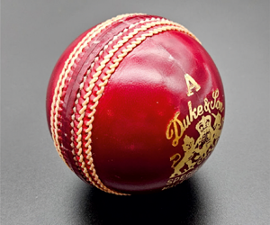
Cricket balls are made from a cork core wrapped in string with a leather casing. A raised, ‘primary’ seam runs around the middle of the ball and perpendicular to this are two tightly stitched ‘quarter seams’. At the start of an innings the ball is in pristine condition with a shiny, lacquered surface and undamaged seams. Figure 1(a) shows a new red ball used in Test Cricket matches in England. As a cricket match progresses the ball wears as it hits the bat and the ground. The leather becomes rough, the raised seam can be damaged or compressed and the quarter seams can begin to split. A worn, white cricket ball used in a One Day International match is shown in figure 1(b).
(a) New red ball used in Test Matches; (b) worn white ball used in a One Day International Match.

1.1 Overview of cricket ball swing literature
Numerous academic papers have been published explaining how the behaviour of the flow immediately adjacent to the ball, called the boundary layer, results in a sideways force which causes the ball to swing. These theories were first presented in the 1950s by Reference CookeCooke (1955) and Reference LyttletonLyttleton (1957) and in the following years, experiments by Reference Harrington and SouthworthHarrington & Southworth (1957), Reference Burgess and ProbertBurgess & Probert (1972) and Reference Moore and NeedesMoore & Needes (1973) were performed to test the ideas. Horlock's 1973 paper (Reference HorlockHorlock 1973) summarises this early work, combining wind tunnel test data with boundary layer theory to explain why cricket balls swing.
Since the 1980s, Mehta has produced three review papers (Reference MehtaMehta 1985, Reference Mehta2005, Reference Mehta2014), and a similar summary paper was also produced by Reference VermaVerma (2015). These consolidate established ideas and identify topics for further study. Over the last ten years, researchers have continued to investigate cricket ball swing using new techniques including infra-red visualisation of surface flow (Reference Scobie, Pickering, Almond and LockScobie et al. 2013), particle image velocimetry (Reference Jackson, Harberd, Lock and ScobieJackson et al. 2020) and computational fluid dynamics (Reference Tom, Ruishikesh, Jose and KumarTom et al. 2013) to uncover further details about swing. However, despite undoubted progress, the impact of academic work on professional cricket has been limited as it has been unable to explain or predict swing as it is observed on the field of play. This discrepancy is illustrated in the next subsection, where ball tracking data from cricket matches are compared with published results obtained from wind tunnel tests.
1.2 Comparison of ball tracking data with wind tunnel measurements
Ball tracking technology, which utilises multiple high-speed video cameras and triangulation software, was introduced to cricket in 2001 to provide information about the trajectory of cricket ball deliveries. It is now widely adopted in international and professional cricket where it aids match officials in decision making, provides statistics and insight for television viewers and is used by teams and players for performance analysis (Reference Owens and DixonOwens & Dixon 2004).
Section 3 in this article shows how a non-dimensional swing force coefficient,  $C_{S}$, is calculated from ball trajectory data and figure 2 demonstrates how the database can be analysed to study trends in the behaviour of cricket ball swing. The parameter $C_{S}$ is defined in (2.1) in § 2, and provides a measure of the force causing the ball to swing; $C_{S}$ has a magnitude, $|C_{S}|$, and direction denoted by its sign, so that increased $|C_{S}|$ corresponds to more swing. A delivery with $C_{S} = 0$ corresponds to a straight delivery which does not swing.
Distribution of swing force coefficient magnitude,  $|C_{S}|$, in Test Match cricket from 2006 to 2018, calculated from ball tracking data for: (a) ball age less than 1 over; (b) ball age between 40 and 80 overs.

Figure 2(a) shows the distribution of  $|C_{S}|$ for 6982 balls delivered in the first ‘over’ (six legal deliveries) of Test Cricket matches between 2006 and 2018, with a release speed greater than 60 mph (27 m s $^{-1}$). The direction of swing is not plotted, as the aim is to capture both ‘in-swing’ and ‘out-swing’ deliveries. The histogram shows that, for new balls, 44 % of deliveries have $|C_{S}|$ less than 0.1, 41 % are between 0.1 and 0.3, and 15 % are greater than 0.3.
Most previous work on cricket ball swing begins by considering the behaviour of new balls. A compilation of  $C_{S}$ results from various studies is presented in figure 6 in § 4. These results are recorded using a ball mounted in a wind tunnel so that $C_{S}$ can be measured. The results of the different wind tunnel tests are consistent; $|C_{S}|$ measured is either high, between 0.2 and 0.35, or low, less than 0.1, and the continuous distribution of $|C_{S}|$ observed on the field and presented in figure 2 is not reproduced.
Figure 2(b) shows the distribution of  $|C_{S}|$ for old balls in Test Cricket. These data comprise 99 913 deliveries released at a speed greater than 60 mph (27 m s $^{-1}$) with a ball aged between 40 and 80 overs old. The histogram shows that the distribution of $|C_{S}|$ is shifted to lower values compared with the opening over shown in figure 2(a): 53 % of deliveries have $|C_{S}|$ less than 0.1, 43 % are between 0.1 and 0.3 and 4 % are larger than 0.3. Measurements of old cricket balls presented in the literature are reproduced in figure 7 in § 4. Unlike new balls, these data show a continuous spread of $|C_{S}|$ between 0 and 0.35, which agrees qualitatively with the ball tracking data for old balls. Our literature review concludes, however, that the mechanisms which produce this spread of $C_{S}$ for old balls has not been fully explained and a quantified relationship between ball condition and swing has not been established.
1.3 Paper aims and layout
This paper provides an up-to-date review and reassessment of published research on cricket ball swing. It also presents new data, including simultaneous force and infra-red (IR) flow visualisation measurements, obtained from wind tunnel tests performed at the Whittle Laboratory in Cambridge, UK. The paper has two objectives: first, it seeks to confirm previously published explanations for cricket ball swing and update these where necessary. Second, it aims to identify topics for further research which will enable the behaviour observed in cricket matches using ball tracking data, for example in figure 2, to be explained and modelled.
The paper is split into five further sections. In § 2, the nomenclature and terminology of cricket ball swing and boundary layers are defined and in § 3 the assumptions and methods used to process the ball tracking data shown in figure 2 are described. Section 4 reviews papers which discuss how cricket ball boundary layer behaviour causes swing and compares published results with new wind tunnel measurements. Section 5 considers papers which have studied realistic boundary conditions which include the effect of ball rotation and atmospheric conditions, and finally, § 6 presents conclusions along with recommendations for future work.
2. Nomenclature and terminology
2.1 Cricket ball swing
As the literature around cricket ball swing has grown, a common nomenclature and terminology has developed which is summarised in figure 3. Here, the ball is viewed from ‘top down’ and the swing and drag forces,  $F_{S}$ and $F_D$, act perpendicular to and in line with the direction of flight, respectively. The seam angle, $\theta$, defines the angle between the seam centre line and direction of flight while the rotation angle, $\alpha$, and rate, $\omega$, are defined perpendicular to the seam centre line. The side of the ball where the flow passes over the seam at the front of the ball is called the ‘seam side’ and the other side is called the ‘non-seam side’. Separation points are quantified by separation angle, $\phi _{s}$ and are measured from the stagnation point at the front of the ball to the point where the boundary layer separates and forms a wake.
Top down view of cricket ball including sketch of streamlines passing the non-seam side and variables related to swing.

In this article, forces are non-dimensionalised by the dynamic pressure acting on the ball as defined in (2.1)
 \begin{equation} C_{S} = \frac{F_{S}}{\dfrac{1}{2} \rho A U^2}, \end{equation}
where  $\rho$ is air density, $A$ is the frontal area of the ball and $U$ is ball speed. Ball geometry, speed and the properties of air are also combined to evaluate the Reynolds number
 \begin{equation} Re = \frac{\rho U D}{\mu}, \end{equation}
where  $D$ is ball diameter and $\mu$ is the dynamic viscosity of air; $Re$ represents the ratio of inertial to viscous forces in a flow and strongly influences boundary layer behaviour, discussed in the next subsection.
There are two types of cricket ball swing: ‘conventional swing’ and ‘reverse swing’. For conventional swing, the swing force acts towards the seam side, and the ball swings in the direction that the seam is pointing, as shown in figure 3. Reverse swing acts in the opposite direction; the swing force is towards the non-seam side and the ball swings away from the direction the seam is pointing. In this paper, swing force is defined as positive for conventional swing and negative for reverse swing in line with other studies.
2.2 Boundary layer behaviour
Publications on cricket ball swing often discuss boundary layers although there is some inconsistency in the terms used in different papers. This subsection defines the terminology for describing boundary layers based on Schlichting's seminal work on the topic (Reference SchlichtingSchlichting 2016).
A boundary layer is the region of flow close to a surface where the flow velocity is slowed by viscous interactions with a ‘no-slip condition’ at the wall. For a cricket ball in flight, the boundary layer is best described in a frame of reference moving with the ball. The ball then appears stationary, with flow approaching at the flight speed and a no-slip condition at the ball surface. Within the boundary layer the flow can be ‘laminar’ or ‘turbulent’ and these different types of boundary layer are illustrated in figure 4. Laminar flow is layered, with sheets of fluid moving ‘with different velocities without great exchange of fluid particles perpendicular to the flow direction’ (Reference SchlichtingSchlichting 2016). Turbulent flow ‘is characterised by a highly irregular, random, fluctuating motion [which is] superimposed on the regular basic flow and leads to large amounts of mixing perpendicular to the flow direction’ (Reference SchlichtingSchlichting 2016). It is the transverse mixing motion which causes momentum exchange normal to the flow direction in turbulent boundary layers.
Illustrations of boundary layer behaviour. Unsteady, turbulent flow is represented by ‘eddies’ superposed over dashed lines. (a) Laminar boundary separation; (b) transition and turbulent boundary layer separation; (c) laminar boundary layer separation and turbulent reattachment.

At low values of  $Re$, flows are laminar but as $Re$ increases above a ‘critical’ value there is a ‘transition’ to turbulent flow. Transition occurs at a point when the boundary layer flow becomes unstable and small disturbances are able to grow and propagate, leading to a turbulent boundary layer. Laminar to turbulent transition in boundary layers is affected by a number of factors alongside $Re$. The most important of these for studying cricket ball swing are the free-stream turbulence and surface roughness.
When a boundary layer forms on a curved surface, such as that of a cricket ball, it experiences a pressure gradient in the streamwise direction. An ‘adverse pressure gradient’ is experienced when the pressure increases in the direction of flow,  $\mathrm {d}p/\mathrm {d}s>0$, and velocity reduces. The deceleration of the boundary layer flow causes it to undergo ‘separation’ when the velocity profile becomes inflected and the velocity gradient at the wall is zero. Downstream of this point, the flow close to the surface reverses and a separation forms, as shown in figure 4. For the same adverse pressure gradient, a turbulent boundary layer remains attached for longer than a laminar boundary layer due to the increased transverse momentum transfer associated with turbulent flow. Adverse pressure gradients also promote turbulent transition as their effect on the velocity profile acts to reduce the stability of a laminar boundary layer.
Under the right conditions, transition can occur in the separated free shear layer downstream of a laminar boundary layer separation, as shown in figure 4(c). A recent review of this topic is provided by Reference YangYang (2019) and this explains that, for low levels of turbulence intensity, <3 %, transition occurs due to an instability in the shear layer growing into fully developed turbulent flow. In the separated flow, the viscous damping is reduced compared with an attached boundary layer causing the transition to turbulence to occur over a shorter streamwise distance. Once the flow is turbulent, the increase in transverse momentum transfer can cause the flow to ‘reattach’ to the surface. When this happens the flow between the separation and reattachment becomes trapped and forms a ‘separation bubble’.
The boundary layer flows observed around cricket balls are characterised by the behaviours described above and illustrated in figure 4. The differences in separation position between laminar, turbulent and reattached turbulent boundary layers is the underlying mechanism for generating a swing force on a cricket ball.
3. Cricket ball trajectories and quantifying swing using ball tracking data
Since 2001, ball speed and position have been recorded during international cricket matches using high-speed cameras and ball tracking software (Reference Owens and DixonOwens & Dixon 2004). This section considers the trajectory of a cricket ball delivery and explains how the ball tracking database is processed to provide force coefficient distributions like that shown in figure 2.
Swing is caused by an aerodynamic force acting in a horizontal plane, perpendicular to the direction of ball flight. A ball's trajectory can therefore be used to determine the forces acting upon it. Figure 5 shows a ball travelling at an average speed  $U$, under the influence of a perpendicular swing force, $F_{S}$. Baker's study on the trajectory of a swinging cricket ball, using time-dependent equations of motion (Reference BakerBaker 2010), shows that the same trajectory is formed when considering either instantaneous or time-averaged values for ball speed and force, provided that the $C_{S}$ and drag force coefficient, $C_D$, remain constant for the time of flight, $t$. The ball tracking database does not provide time accurate positions or velocities between release and bounce, so a constant $C_{S}$ and average speed are assumed for the entire delivery. Equations (3.1) and (3.2) show how this analysis produces a parabolic trajectory for a ball travelling a distance $l$ along its initial trajectory, while swinging a distance, $s$. Here, $m$ is ball mass equal to 0.156 kg and $a$ is the ball acceleration perpendicular to its direction of flight
 \begin{equation} s = \frac{1}{2}a t^2 = \frac{F_{S}}{2m}t^2.\end{equation}
Top down view of cricket pitch showing ball trajectory and variables recorded by ball tracking.

Combining (3.1) with (2.1) for the non-dimensional swing force coefficient allows the perpendicular displacement,  $s$, to be defined in terms of $C_{S}$
 \begin{equation} s = \frac{\rho A U^2 C_{S}}{4m}\frac{l^2}{U^2} = \frac{\rho A}{4m}C_{S} l^2.\end{equation}
 The relationship between swing force and ball trajectory means that the ball tracking database can be used to calculate an average  $C_{S}$; $C_{S}$ can also be measured in wind tunnel experiments and compared directly with values calculated from ball tracking data. Figure 5 shows the parameters recorded: the position of ball release, $x_{r}$ and $y_{r}$, and bounce, $x_{b}$ and $y_{b}$, the ball speed at release, $U_{r}$, and when it bounces, $U_{b}$, and the ‘degree of swing’, $\beta _{S}$, which is the change in angle in the $x$–
$x$– $y$ plane of the ball trajectory between release and bounce. Noting that $\beta _{S} < 5^{\circ }$ gives an expression for $s/l$
$s/l$
 \begin{equation} \frac{s}{l} =
\tan\Big(\frac{\beta_{S}}{2}\Big) \approx
\frac{\beta_{S}}{2}.\end{equation}
\begin{equation} \frac{s}{l} =
\tan\Big(\frac{\beta_{S}}{2}\Big) \approx
\frac{\beta_{S}}{2}.\end{equation}
Combining (3.2) and (3.3) gives an expression for  $C_{S}$ which can be calculated using the values recorded for each delivery in the ball tracking database
 \begin{equation} C_{S} = \frac{2m}{\rho A}\frac{\beta_{S}}{l}.\end{equation}
 The ball mass and frontal area are those specified by the laws of the game and where atmospheric conditions are not recorded, the standard value for air density is used, leading to an error of up to  $\pm$10 %. Unlike degree of swing, $C_{S}$ is independent of ‘length’, the distance between release and bounce, and is also normalised for air density if atmospheric conditions are recorded.
4. Boundary layer aerodynamics and cricket ball swing
Since the 1970s, researchers have measured swing force using cricket balls mounted on a sting in a wind tunnel. Results showing  $C_{S}$ against $Re$ for new cricket balls, from Reference Scobie, Shelley, Jackson, Hughes and LockScobie et al. (2020), Reference Deshpande, Shakya and MittalDeshpande, Shakya & Mittal (2018), Reference Sayers and HillSayers & Hill (1999) and Reference Alam, Hillier, Xia, Chowdhury, Moria, La Brooy and SubicAlam et al. (2010b) are reproduced in figure 6. Old balls, which have been worn through use in a cricket match (Reference Scobie, Pickering, Almond and LockScobie et al. 2013, Reference Scobie, Shelley, Jackson, Hughes and Lock2020; Reference Tadrist, Sampara, Ashraf and AndrianneTadrist et al. 2020) or aged artificially using sandpaper (Reference Deshpande, Shakya and MittalDeshpande et al. 2018), have also been investigated and results from these experiments are shown in figure 7. Included in both figures are measurements performed for this review paper which are labelled ‘W’. The experimental methods used to obtain the Whittle Laboratory data are detailed in Appendix A.
Swing force coefficient,  $C_{S}$, for new cricket balls plotted against Reynolds number, $Re$, for experiments reported by Reference Scobie, Shelley, Jackson, Hughes and LockScobie et al. (2020): A,B,C; Reference Deshpande, Shakya and MittalDeshpande et al. (2018): D,E; Reference Sayers and HillSayers & Hill (1999): F; Reference Alam, Hillier, Xia, Chowdhury, Moria, La Brooy and SubicAlam et al. (2010b): G; and from Whittle Laboratory tests: H,I. The IR images for conventional swing are presented in figure 12 for the three cases highlighted with solid circular markers, and IR images for reverse swing are presented in figure 16 for the case highlighted with a solid square marker.

Swing force coefficient,  $C_S$, for used cricket balls plotted against Reynolds number, $Re$, for experiments reported by Reference Scobie, Shelley, Jackson, Hughes and LockScobie et al. (2020): A,B,C,D; Reference Scobie, Pickering, Almond and LockScobie et al. (2013): E,F,G; Reference Deshpande, Shakya and MittalDeshpande et al. (2018): H,I; Reference Tadrist, Sampara, Ashraf and AndrianneTadrist et al. (2020): J,K; and from Whittle Laboratory tests: L,M,N. The IR images for reverse swing are presented in figure 16 for the two cases highlighted with solid square markers.

The new ball measurements shown in figure 6 all exhibit similar behaviour with two regimes observed: when  $Re$ is below a specific value for each ball, $C_{S}$ between 0.25 and 0.35 is recorded, with the positive sign indicating conventional swing. For $Re$ above the specific value, a smaller, negative $C_{S}$ of between $-$0.05 and $-$0.12 is recorded, indicating reverse swing. From a cricketing perspective, $Re=1.8\times 10^5$ corresponds to a bowling speed of approximately 85 mph, at standard atmospheric conditions of air density 1.225 kg m $^{-3}$ and viscosity $1.8\times 10^{-5}$ kg m $^{-1}$ s $^{-1}$. At this speed, deliveries with $C_{S}=0.3$ swing towards the seam side 0.52 m if bouncing 15 m from release.
For old balls, shown in figure 7, there is more variation in the results. Balls A,B,C,E,H,J and K have positive  $C_{S}$ varying between 0.1 and 0.45 for $Re$ below a specific value for each ball. At higher $Re$ these balls display reverse swing with negative values of $C_{S}$ between $-$0.1 and $-$0.3. Balls D,F,G and I, which are older or artificially worn on both sides, have $C_{S}$ between 0.1 and $-$0.1 and have undergone the switch from conventional to reverse swing at $Re$ below the range encountered in professional cricket.
Most published work on cricket ball aerodynamics attempts to explain the behaviours observed in figures 6 and 7 by studying the flow past the non-seam and seam side of the ball and by considering how the changes in boundary layer behaviour cause the ball to swing. This section of our review summarises the literature and compares published results with new data recorded for this paper. Where necessary, physical explanations are refined or updated and previous measurements reassessed based on the new analysis. The discussion is split into five parts: the first subsection covers conventional swing, the second reviews reverse swing, the third considers the switch from conventional to reverse swing, the fourth covers the two-dimensional approximation implicit in most explanations of cricket ball swing and the fifth provides a summary and lists areas for further study.
4.1 Conventional swing
Horlock's paper (Reference HorlockHorlock 1973), which reports cylinder and cricket ball wind tunnel tests, is the first to show that conventional swing is caused by ‘laminar separation on the smooth [non-seam] side and turbulent separation on the rough [seam] side’. Figure 8(a), reproduced from Reference MehtaMehta (1985), confirms the asymmetric nature of the flow with different separation points observed on the non-seam and seam sides using smoke flow visualisation. It should be noted that this test was performed at  $Re = 0.85\times 10^5$, approximately half of that encountered in professional cricket. Similar results, showing separation asymmetry but at higher $Re$ have been obtained by Reference Deshpande, Shakya and MittalDeshpande et al. (2018), where oil flow visualisation was used on an aluminium model of a cricket ball as shown in figure 8(b), Reference Scobie, Pickering, Almond and LockScobie et al. (2013), who used IR imaging on a model cricket ball as shown in figure 8(c) and Reference Jackson, Harberd, Lock and ScobieJackson et al. (2020) who present a top down view of the flow past a model ball using particle image velocimetry (PIV) as shown in figure 8(d). Figure 9, reproduced from Reference Scobie, Pickering, Almond and LockScobie et al. (2013), shows pressure measurements around an instrumented model cricket ball at $Re = 0.20\times 10^5$, $1.47\times 10^5$ and $1.95\times 10^5$, assuming standard atmospheric conditions. These measurements allow the authors to estimate the position of separation points on each side and also demonstrate the asymmetric nature of the flow past the ball.
Flow visualisation experiments from the literature illustrating asymmetric separation points for conventional swing. (a) Smoke flow visualisation at  $Re = 0.85\times 10^5$ (Reference MehtaMehta 1985); (b) oil flow visualisation on an aluminium model ball at $Re=2.82\times 10^5$ (Reference Deshpande, Shakya and MittalDeshpande et al. 2018); (c) IR imaging of a model cricket ball at $Re=1.47\times 10^5$ (Reference Scobie, Pickering, Almond and LockScobie et al. 2013). Red indicates a separated region where heat transfer from the free-stream flow to the ball is low; (d) PIV measurement of model cricket ball at $Re=1.1\times 10^5$ (Reference Jackson, Harberd, Lock and ScobieJackson et al. 2020). Yellow contours indicate high velocity, dark blue contours indicate zero velocity.

Variation of pressure coefficient with angle from stagnation point at varying speed (Reference Scobie, Pickering, Almond and LockScobie et al. 2013); NS: no swing, CS: conventional swing, RS: reverse swing. Assuming standard atmospheric conditions, 9 mph is equivalent to  $Re=0.20\times 10^5$, 67 mph is equivalent to $Re=1.47\times 10^5$ and 89 mph is equivalent to $Re=1.95\times 10^5$.

Research by Reference AchenbachAchenbach (1972, Reference Achenbach1974) into the flow past spheres is referenced in several cricket ball swing papers (Reference BentleyBentley 1982; Reference Scobie, Pickering, Almond and LockScobie et al. 2013, Reference Scobie, Shelley, Jackson, Hughes and Lock2020; Reference Jackson, Harberd, Lock and ScobieJackson et al. 2020; Reference Tadrist, Sampara, Ashraf and AndrianneTadrist et al. 2020) and figure 10 reproduces Achenbach's results showing separation angle plotted against Reynolds number for spheres with three levels of roughness. For the smooth sphere, the separation point in the sub-critical regime where  $Re<2\times 10^5$ is $82^{\circ }$. This increases to around $120^{\circ }$ in the super-critical regime where $Re>4\times 10^5$. Reference Scobie, Shelley, Jackson, Hughes and LockScobie et al. (2020) combine their cricket ball measurements with Achenbach's results for spheres, to provide an explanation of conventional swing which is illustrated by the sketch in figure 11.
Variation of separation angle with Reynolds number for spheres with varying roughness. Reproduced from Reference AchenbachAchenbach (1974).

Top down sketch of flow past a cricket ball for conventional swing. Reproduced from Reference Scobie, Shelley, Jackson, Hughes and LockScobie et al. (2020).

To validate Scobie et al.'s description of conventional swing, IR images of the non-seam and seam sides of a new cricket ball, at  $Re$ values which result in conventional swing, have been captured at the Whittle Laboratory in Cambridge, UK. A temperature difference between the ball surface and the flow is achieved by chilling the ball to $5\,^{\circ }$C, meaning that areas of low heat transfer appear light, as the surface remains colder than the wind tunnel jet, and regions of high heat transfer appear dark, as the surface is heated by the wind tunnel flow. A description of the experimental methods used to obtain these images is provided in Appendix A. The rest of this subsection on conventional swing is split into an analysis of the flow over the non-seam side, then the seam side, before finally assessing the flow asymmetry.
4.1.1 Non-seam side
Figure 12(a) shows that on the non-seam side of the ball there is a white stripe caused by a flow separation. The flow separates at the front of this stripe and the recirculating flow, trapped beneath the separated shear layer, has low heat transfer so the surface of the ball remains cold. This result agrees with Scobie et al.'s sketch for the non-seam side shown in figure 11 and confirms that the separation angle on this side of the ball is approximately  $80^{\circ }$. Figure 12(a–c) also shows that the position of the laminar separation on the non-seam side does not change between $Re=1.42\times 10^5$ and $Re=1.89\times 10^5$. This agrees with Achenbach's result for a smooth sphere, figure 10, which shows that the separation angle remains constant at $82^{\circ }$ for cases where $Re$ is below the critical value.
Seam and non-seam side IR images of a new, red Dukes cricket ball, ball I in figure 6, undergoing conventional swing at varying Reynolds number. Flow is left to right and red dashed lines illustrate eventual separation position.

Measurements using model balls instrumented with pressure tappings by Reference Scobie, Pickering, Almond and LockScobie et al. (2013), see figure 9, and Reference Deshpande, Shakya and MittalDeshpande et al. (2018), have also shown that the separation on the non-seam side occurs at approximately  $80^{\circ }$. Figure 8(d) from Reference Jackson, Harberd, Lock and ScobieJackson et al. (2020) shows that the separation angle on the non-seam side at $Re=1.1\times 10^5$ is $95^{\circ }$. The authors explain that this is because the surface roughness is greater than a new ball and links this to Achenbach's roughened sphere results in figure 10. For the separation angle to increase to $95^{\circ }$ implies that transition has begun but this idea is not discussed. It is also noted that the model ball tested by Jackson et al. is a replica of the one used for the measurements in figure 9. The roughness of these balls is reported to be the same, however, Scobie et al.'s tests at $Re=0.20\times 10^5$ and $Re=1.47\times 10^5$ both show a laminar separation at approximately $80^{\circ }$. The discrepancy between these results and the PIV result in figure 8(d) is not explained.
4.1.2 Seam side
Existing publications discussing cricket ball swing often state that the boundary layer on the seam side is ‘tripped’ to turbulence by the seam. Indeed, Reference HorlockHorlock (1973), Reference Deshpande, Shakya and MittalDeshpande et al. (2018) and Reference SayersSayers (2001) test model cricket balls where the seam is represented by a wire trip. Reference Son, Choi, Jeon and ChoiSon et al. (2011) describe two ways in which a wire trip can delay boundary layer separation and reduce drag: first, the disturbance from the trip can cause transition along the separated shear layer resulting in a separation bubble and turbulent reattachment. Alternatively, disturbances from the trip can cause transition to turbulence before separation, with no separation bubble formed. Deshpande et al. are the only authors to suggest the presence of a laminar separation bubble on the seam side, while others state that the boundary layer is tripped with no mention of a separation bubble.
Another description of the flow on the seam side of the ball, provided by Reference Scobie, Shelley, Jackson, Hughes and LockScobie et al. (2020) and Reference Jackson, Harberd, Lock and ScobieJackson et al. (2020), links the seam side behaviour to the rough sphere in figure 10 (black line with square symbols) so that, for conventional swing, the seam side boundary layer separates further back on the ball than the smooth, non-seam side (red line). Achenbach's data for the rough sphere show a separation angle of  $100+/-5^{\circ }$ in the range $Re=1-2\times 10^5$. However, Jackson's PIV measurement of a model cricket ball, figure 8(d), and Scobie et al.'s measurements using an instrumented model ball, figure 9, show a separation angle of $120+/-5^{\circ }$. This is the value used in the diagram in figure 11. The difference between the rough sphere and cricket ball experiments is not discussed and we conclude that Achenbach's rough sphere results are unsuitable for modelling the seam side of a cricket ball, since the separation angles differ by approximately $20^{\circ }$.
Figure 12(d–f) presents Whittle Laboratory IR images of the seam side of the ball for conventional swing at varying  $Re$. These results show streamwise ‘streaks’ on the front half of the ball, which are caused by coherent structures shed by the seam. These appear dark in the image, where warm flow from the free stream is mixed down to the cool surface of the ball, implying that the seam acts more like a row of vortex generators than a wire trip. Just behind the midpoint of the ball there is a laminar separation bubble, indicated by the white stripe in the IR images. The separation bubble is closed with a turbulent boundary layer reattachment, shown by the dark region of high heat transfer, before the flow eventually separates towards the back of the ball.
The results in figure 12 show that streamwise flow structures are involved in the separation and reattachment of the boundary layer flow on the seam side. This type of behaviour is widely reported in the literature outside of cricket ball aerodynamics, and reviews are provided by Reference Gad-El-Hak and BushnellGad-El-Hak & Bushnell (1991) and Reference YangYang (2019). Much of this ‘boundary layer control’ research is concerned with improving the performance of aircraft wings, however, Reference Joubert and HoffmanJoubert & Hoffman (1962) show that vortex generators placed along a cylinder,  $20^{\circ }$ from the stagnation point, are able to reduce drag by 50 % at $Re=1.3\times 10^5$ compared with a smooth cylinder. We hypothesise that the cylinder drag reduction measured by Joubert et al. is due to the same kind of flow physics seen in figure 12(d–f): the coherent streamwise structures shed by the seam/vortex generators interact with the separated shear layer causing transition, a turbulent boundary layer reattachment and eventual separation towards the rear of the ball/cylinder. This is different to the wire trip or rough sphere mechanisms where transverse perturbations cause the transition to turbulence.
Flow visualisation and pressure tapping measurements by Reference Deshpande, Shakya and MittalDeshpande et al. (2018) also indicate the presence of a laminar separation bubble on the seam side. However, these results appear to have been overlooked by other researchers since they are recorded using an aluminium model ball, where the switch from conventional to reverse swing does not occur until approximately  $Re=4\times 10^5$, an unrealistically high value for cricket. Scobie et al.'s measurements in figure 9, show that at $Re=1.47\times 10^5$ (labelled CS – 67 mph) there is a flattening of the pressure profile between $80^{\circ }$ and $90^{\circ }$ on the seam side. This is indicative of a laminar separation bubble, however, this feature is not discussed in Scobie et al.'s paper (Reference Scobie, Pickering, Almond and LockScobie et al. 2013) or the same group's subsequent work (Reference Jackson, Harberd, Lock and ScobieJackson et al. 2020; Reference Scobie, Shelley, Jackson, Hughes and LockScobie et al. 2020).
Overall, the description of seam side flow for conventional swing, summarised in figure 11, where the seam is said to trip the boundary layer, should be updated. The IR images in figure 12, supported by previous pressure tapping measurements (Reference Scobie, Pickering, Almond and LockScobie et al. 2013; Reference Deshpande, Shakya and MittalDeshpande et al. 2018), show that coherent streamwise structures are shed from the seam and that these cause a turbulent reattachment behind a laminar separation bubble.
4.1.3 Flow asymmetry
Combining the descriptions for the non-seam and seam sides leads to an updated explanation for conventional swing. Figure 13 shows a top down sketch of the flow past a cricket ball. The laminar separation on the non-seam side was hypothesised in the earliest papers on cricket ball swing in the 1950s and has been shown to occur at approximately  $80^{\circ }$ when $Re$ is below the critical value for that side of the ball.
Top down sketch of flow past a cricket ball for conventional swing updated using Whittle Laboratory results.

On the seam side, established explanations that the boundary layer transitions to turbulence because the seam acts like a wire trip, or that the seam side behaves like a rough sphere, should be revised. Figure 13 shows coherent streamwise structures, shed from the seam, which close a separation bubble and result in a turbulent boundary layer separation at approximately  $120^{\circ }$.
The asymmetry in the boundary layer separation results in a sideways force which causes the ball to swing in the direction that the seam is pointing. While the non-seam side flow is below a critical  $Re$, the separation points on both sides of a new ball do not change greatly for $Re=1.42\times 10^5$ to $Re=1.89\times 10^5$, as shown in figure 12. This explains why $C_{S}$, shown in figure 6 for new balls, does not vary significantly, e.g. for a new red Dukes ball, tested at the Whittle Laboratory, there is less than 5 % variation in $C_{S}$ between $Re=1.42\times 10^5$ and $Re=1.92\times 10^5$. Figure 7 shows that used balls can also exhibit conventional swing with $C_{S}$ between 0.2 and 0.35, however, the switch to reverse swing occurs at lower $Re$ and is less sudden than for new balls. This is because a roughened non-seam side transitions more gradually and at lower $Re$, as shown for rough spheres by Achenbach in figure 10.
4.2 Reverse swing
Reverse swing occurs when  $C_{S}$ is negative so that the ball deviates away from the direction that the seam is pointing. Figure 6 shows that new balls, with $Re$ above a specific value, have a negative $C_{S}$ of $-$0.05 to $-$0.1. For old balls, shown in figure 7, reverse swing occurs at lower $Re$ and $C_{S}$ varies between 0 and $-$0.4.
The first reference in the literature to a behaviour now recognised as reverse swing was made by Reference HorlockHorlock (1973) who noted that ‘The presence of the secondary [quarter] seam appears to cause transition on the smooth [non-seam] side in some cases and may cause small or even negative lift’. He explains that this is because  $Re$ is greater than the critical value on both the non-seam and seam side causing both to transition to turbulence. Reference MehtaMehta (1985) builds on this idea and hypothesises that the seam causes the separation on the seam side to occur further forwards than the non-seam side which switches the direction of the swing force compared with conventional swing.
Further studies on reverse swing, reproduced in figure 14, have provided experimental evidence to support Mehta's idea. Reference Deshpande, Shakya and MittalDeshpande et al. (2018) show oil flow visualisation on an aluminium sphere with trip wire representing the seam as shown in figure 14(a), Reference Scobie, Pickering, Almond and LockScobie et al. (2013) study a model ball using IR visualisation as shown in figure 14(b) and Reference Jackson, Harberd, Lock and ScobieJackson et al. (2020) provide a top down view of the flow past a model ball using PIV as shown in figure 14(c). These results highlight the presence of a laminar separation bubble and turbulent reattachment on the non-seam side and figure 15, reproduced from Reference Scobie, Shelley, Jackson, Hughes and LockScobie et al. (2020), consolidates these results to provide the most recent description of reverse swing.
Flow visualisation experiments from the literature illustrating flow past the ball for reverse swing with flow moving from left to right. (a) Oil flow visualisation on an aluminium model ball at  $Re=3.92\times 10^5$ (Reference Deshpande, Shakya and MittalDeshpande et al. 2018); (b) IR imaging of a model cricket ball at $Re=1.95\times 10^5$ (Reference Scobie, Pickering, Almond and LockScobie et al. 2013). Red indicates a separated region where heat transfer from the free-stream flow to the ball is low; (c) PIV measurement of model cricket ball on non-seam side at $Re=1.74\times 10^5$ (Reference Jackson, Harberd, Lock and ScobieJackson et al. 2020). Yellow contours indicate high velocity, dark blue contours indicate zero velocity.

Top down sketch of flow past a cricket ball for reverse swing. Reproduced from Reference Scobie, Shelley, Jackson, Hughes and LockScobie et al. (2020).

Figure 7 shows  $C_{S}$ for old balls varying between 0 and $-$0.4. This is due to differences in the separation asymmetry between the two sides of the ball with the largest force obtained when the seam side separation is as far forward as possible, and the non-seam side separation is as far back as possible. The rest of this section reviews boundary layer behaviour on each side of the ball in order to assess the explanations given in the literature and to understand why reverse swing magnitude varies more than conventional swing. The literature review is supplemented by figure 16, which shows IR images captured in Whittle Laboratory experiments for three balls which have negative $C_{S}$.
Seam and non-seam side IR images of three cricket balls undergoing reverse swing. Flow is left to right and red dashed lines illustrate eventual separation position. (a) New ball with shiny seam and non-seam sides, ball I in figure 6; (b) ‘doctored’ ball with rough seam side and shiny non-seam side, ball M in figure 7; (c) used ball with rough seam and non-seam sides, ball N in figure 7.

4.2.1 Non-seam side
On the non-seam side, figure 15 shows that the laminar boundary layer separates at  $95^{\circ }$, forms a laminar separation bubble, reattaches as a turbulent boundary layer and then separates to form a wake at $135^{\circ }$. This explanation is based on several measurements reported in the literature: figure 9 shows that at $Re=1.95\times 10^5$ (89 mph – RS), a constant pressure is recorded between $-90^{\circ }$ and $-100^{\circ }$, indicating the presence of a separation bubble; figure 14(a) shows a laminar separation bubble on the non-seam side using oil flow visualisation; the red region on the non-seam side in figure 14(b) indicates a separation bubble and reattachment; and in figure 14(c) PIV measurements show a laminar separation, reattachment and eventual turbulent separation at $130^{\circ }$. The Whittle Laboratory IR image of the non-seam side of the new ball in figure 16(a) matches the flow mechanism sketched in figure 15: the white stripe followed by a dark region indicates a laminar separation bubble and turbulent reattachment. These results agree qualitatively with Achenbach's measurements (Reference AchenbachAchenbach 1974) for smooth spheres above a critical $Re$ of $2\unicode{x2013}3\times 10^5$, shown in figure 10, where the flow becomes turbulent in the shear layer of the laminar separation, causing a turbulent boundary layer to reattach then finally separate at $120^{\circ }$.
Figure 16(c) shows an IR image of the non-seam side of a ball artificially roughened to represent an old ball. Roughness is generated with a sand blaster and is measured using a profilometer to be  $k/D = 55\times 10^{-5}$ for the cases shown in figure 16(c,e,f), where $k$ is the peak-to-peak value of the surface profile. Further details of the generation and measurement of surface roughness are given in Appendix A. Visualisation for this condition has not been presented in the literature before, although force measurements for old or artificially roughened balls, are reproduced in figure 7. In figure 16(c), a region of laminar flow, which appears light grey because the heat transfer coefficient is low, is observed at the front of the ball. The surface roughness then causes the boundary layer to become turbulent, there is no laminar separation bubble and the turbulent separation is moved forwards compared with the new ball case shown in figure 16(a). This behaviour is consistent with Achenbach's results in figure 10, where the separation angle for the rough spheres are 10– $20^{\circ }$ further forwards than for the smooth sphere for cases where $Re$ is above the critical value.
Scobie et al.'s sketch of the non-seam side flow in figure 15 captures the case when the ball is new or its shine has been maintained. However, a second drawing is required to describe the non-seam side flow as the ball becomes older and more worn and the separation point moves forwards.
4.2.2 Seam side
Figure 15 shows a turbulent boundary layer separation on the seam side at  $110^{\circ }$ and this is also labelled on the pressure measurements shown in figure 9 for the reverse swing case. As with the conventional swing results, Reference Scobie, Pickering, Almond and LockScobie et al. (2013) do not discuss the flattening of the pressure profile observed between $80^{\circ }$ and $90^{\circ }$ which suggests the presence of a laminar separation bubble.
The Whittle Laboratory IR image in figure 16(d) shows that the seam side behaviour of a new ball at  $Re=1.95\times 10^5$ is similar to that in the conventional swing regime at $Re=1.89\times 10^5$, shown in figure 12, with streaks shed from the seam, a separation bubble, turbulent reattachment and eventual separation. This is consistent with the flattened pressure profile between $80^{\circ }$ and $90^{\circ }$ seen in figure 9 for reverse swing.
Figure 16(e,f) shows IR images of the seam side of the ball for cases where artificial roughening has been applied. Here, the roughness causes the boundary layer to be turbulent towards the front of the ball, there is no separation bubble and turbulent reattachment and the separation point is moved forward compared with the new ball case shown in figure 16(d). This result is similar to the flow visualisation on the seam side shown in figure 14(a,b). The coherent structures shed from the seam are not as clear in figure 16(e,f) as the other seam side cases. This is because the rough surface causes a turbulent boundary layer to develop and the heat transfer coefficient is increased. This reduces the contrast in heat transfer caused by the coherent flow structures so the streaks are not as noticeable in the IR image. The geometry of the seam is not changed by the roughening process used here so flattening or damaging the seam is not responsible for the streaks being less visible and the changes in measured force coefficient.
Scobie et al.'s seam side sketch of the flow in figure 15 should be updated to include a laminar separation bubble for cases where the ball is new or its shine has been maintained. A second sketch is required to describe the seam side flow as the surface becomes older and more worn and the separation point moves forwards.
4.2.3 Flow Asymmetry
Measurements of swing force coefficient for old balls, collated in figure 7, show that reverse swing magnitude varies more than conventional swing magnitude. This is due to the different conditions shown in figure 16 which ‘bracket’ the boundary layer behaviours that can occur on each side of the ball. To illustrate this, top down sketches of the flow are presented in figure 17 for the three cases recorded in figure 16.
Top down sketches of flow past a cricket ball for reverse swing updated using Whittle Laboratory results. (a) New ball with shiny seam and non-seam sides; (b) doctored ball with rough seam side and shiny non-seam side; (c) used ball with rough seam and non-seam sides.

For a new ball which reverse swings, the separation on both sides is towards the back; the seam side separation is slightly in front of the non-seam side, resulting in a small  $C_{S}$ of $-$0.08. With the doctored ball, the separation point on the seam side is brought forward by roughness, increasing the asymmetry and resulting in $C_{S}=-0.31$. For the old ball, the separation on the non-seam side has also moved forwards, meaning that the asymmetry is reduced so that $C_{S}$ is only $-$0.09. This updated model for reverse swing, shown in figure 17, allows previous literature results, including real and model balls, to be reassessed and grouped.
Different brands of new ball tested by Reference Scobie, Shelley, Jackson, Hughes and LockScobie et al. (2020) and Reference Deshpande, Shakya and MittalDeshpande et al. (2018), balls A–E in figure 6, have shiny seam and non-seam sides and  $C_{S}$ between 0 and $-$0.1 above a critical $Re$. The sketch in figure 17(a) captures these balls’ behaviour.
The model ball tested by Reference Scobie, Pickering, Almond and LockScobie et al. (2013) and Reference Jackson, Harberd, Lock and ScobieJackson et al. (2020) has a laminar separation bubble on the non-seam side, as shown with pressure measurements in figure 9 and PIV in figure 14. No PIV visualisation of the seam side is provided, however, there is evidence in figure 9 of a laminar separation bubble, as discussed above. The model ball's roughness is said to represent 25 overs of wear and  $C_{S}$ is measured to be between $-$0.12 and $-$0.18. Similarly, the 8–10 and 25 over old balls, labelled A and B in figure 7, have $C_{S}$ between $-$0.1 and $-$0.13 for $Re>1.8\times 10^5$. These balls are likely to sit somewhere between the sketches in figure 17(a) and figure 17(b), where the laminar separation bubble on the non-seam side is present but the separation point on the seam side is moved forwards, compared with a new ball, due to roughness. For these cases, reverse swing magnitude could be increased by roughening the seam side more to bring the separation point further forward.
Reference Deshpande, Shakya and MittalDeshpande et al. (2018) also tested a seam side roughened ball, ball H in figure 7, which has  $C_{S}$ around $-$0.2 for $Re>1.95\times 10^5$. This test is similar to the doctored ball shown in figure 16(b) so will have behaviour represented by the sketch in figure 17(b). Old balls provided by a professional cricket team and tested by Reference Scobie, Pickering, Almond and LockScobie et al. (2013), balls E–G in figure 7, have swing force coefficients between $-$0.2 and $-$0.3 and are likely to sit with this group as well. Reference Tadrist, Sampara, Ashraf and AndrianneTadrist et al. (2020) measured swing force coefficients between $-$0.22 and $-$0.34 at $Re=2.4\times 10^5$ for cricket balls at $0^{\circ }$ seam angle with one side roughened and the other left as new, balls J and K in figure 7. These tests are also best represented by the sketch in figure 17(b).
Old balls tested by Reference Scobie, Shelley, Jackson, Hughes and LockScobie et al. (2020), have swing force coefficients between 0 and  $-$0.1, for example ball D in figure 7. Photographs of these balls show they are worn on both sides, with prominent gaps in the quarter seam, and they are therefore likely to behave as shown in figure 17(c). Reference Deshpande, Shakya and MittalDeshpande et al. (2018) tested a ball where both sides were artificially roughened, resulting in swing force coefficients between 0 and 0.1 for $Re>2\times 10^5$; this is ball I in figure 7. The behaviour of this ball is best captured by figure 17(c), but where the non-seam side is rough enough to move its separation point in front of the seam side, causing a small, positive swing force.
Our updated model allows the reverse swing magnitude to be linked to a range of ball conditions. However, the quantified relationship between surface roughness,  $Re$ and separation angle on both sides of the ball, has not been investigated systematically and this represents an area for future work.
4.3 Switch from conventional to reverse swing
Figure 6 shows that the switch from conventional to reverse swing for a new ball measured in a wind tunnel occurs with a change in  $Re$ of less than 5 %. This is due to the sudden increase in separation angle on the non-seam side as flow changes from the sub-critical to super-critical regime. Figures 6 and 7 also show that there is variation in $Re$ at which the change occurs, with old balls switching at $Re<1.5\times 10^5$ and new balls switching at up to $Re=2.15\times 10^5$.
Differences in experimental set-up from study to study are likely to account for some of the variation observed, e.g. how the ball is mounted, blockage factor and free-stream turbulence intensity of the wind tunnel. However, different balls tested by Reference Scobie, Shelley, Jackson, Hughes and LockScobie et al. (2020) are assumed to share the same set-up, and this is also the case for balls tested at the Whittle Laboratory for this paper.
Surface roughness changes the  $Re$ at which the laminar separation on the non-seam side reattaches, as shown in figure 10 for spheres with different levels of roughness. Reference Jackson, Harberd, Lock and ScobieJackson et al. (2020) estimate that the roughness of a new ball is in the range $0< k/D<250\times 10^{-5}$. Reference Tadrist, Sampara, Ashraf and AndrianneTadrist et al. (2020) repeatedly measure the surface roughness of a ball as it is used. Values of $k/D=8.5\times 10^{-5}$ are reported for a new ball and this increases to $k/D=100\times 10^{-5}$ as it becomes worn. A new red Kookaburra ball measured at the Whittle Laboratory has $k/D=14\times 10^{-5}$ on the lacquered surface, while the artificially roughened ball shown in figure 16 has $k/D=55\times 10^{-5}$. Balls made by Kookaburra, Dukes and SG are lacquered when new and not expected to have significantly different levels of surface roughness, although this should be quantified. The different brands have different seam geometries, however, this does not affect the switch from sub-critical to super-critical regimes on the non-seam side. Despite this, the results in figure 6 for new ball swing show a variation in $Re$ at which the switch from conventional to reverse swing happens of $Re=1.8\times 10^5$– $2.15\times 10^5$.
As well as uniform surface roughness, new cricket balls have small ‘defects’ on both sides of the ball. Reference HorlockHorlock (1973) comments that the quarter seam can cause boundary layer transition on the non-seam side and Reference BentleyBentley (1982) also identify the quarter seam and logo as features which increase the ‘effective roughness’ of the ball. More recently, Reference Scobie, Shelley, Jackson, Hughes and LockScobie et al. (2020) compared three types of new ball using the same experimental set-up; these results are reproduced in figure 6. They comment that the difference between the red and pink Dukes balls are ‘probably caused by slight differences in the surface texture’, while the most prominent difference with the white Kookaburra, which switches from conventional to reverse at a lower  $Re$, is due to ‘a prominent secondary seam [quarter seam]’ which has a 0.5 mm gap. These existing discussions of surface condition are mainly qualitative, therefore quantifying cricket ball surface roughness and defects, and establishing a relationship to $Re$ at which conventional swing switches to reverse swing should be an area for future study.
The effect of defect position on cricket ball swing has not been studied, however, Reference ScheweSchewe (1986) investigated the sensitivity of boundary layer flow to small perturbations close to critical  $Re$, on a cylinder. The boundary layer across the entire cylinder length was made to transition by protruding a pin, with a height 1 % of the cylinder diameter, into the flow at the centre of the cylinder. For transition to occur reliably, the pin had to be positioned at $\phi _{s}=45$– $60^{\circ }$. Schewe concludes that ‘ $\ldots$ in the vicinity of a critical state, a very small cause can have a very great effect’, indicating that small defects on a cricket ball can be expected to switch the whole flow regime if they are in the correct location on the ball.
Reference Sayers and HillSayers & Hill (1999) show a variation in swing force of approximately 15 % for seam angles of  $10^{\circ }$, $30^{\circ }$ and $50^{\circ }$. However, these wind tunnel tests are performed at $Re<1.7\times 10^5$, which is not high enough to show the effect on non-seam side transition. Reference Deshpande, Shakya and MittalDeshpande et al. (2018) test a new cricket ball at $10^{\circ }$, $20^{\circ }$ and $30^{\circ }$ and show that the $10^{\circ }$ and $30^{\circ }$ cases switch from conventional to reverse swing at $Re$ values within 5 % of each other. However, the $20^{\circ }$ case switches at $Re$ around 35 % below the $10^{\circ }$ case. Similar results are presented by Reference Shah and MittalShah & Mittal (2023), who report a variation of approximately 25 % in the $Re$ at which the switch occurs for cases with seam angles of $10^{\circ }$ and $20^{\circ }$. Neither paper provides an explanation for this behaviour, however, we hypothesise that differences observed at specific seam angles are due to a defect on the ball moving to a position which causes early transition.
Reference BartonBarton (1982) measures  $C_{S}$ for a new ball and a ball used for 10 overs at seam angles of $15^{\circ }$ and $30^{\circ }$ up to $Re=1.32\times 10^5$. For the new ball, increasing seam angle reduces the peak $C_{S}$ from 0.36 to 0.31 and reduces $Re$ at which the sudden drop in $C_{S}$ occurs. The same trends are observed for the 10 over old ball although $C_{S}$ is reduced compared with the new ball. An additional test at seam angle of $0^{\circ }$ for the 10 over old ball results in a maximum $C_{S}$ of 0.38. For this case, Barton concludes that the quarter seam, oriented perpendicular to the flow direction on one side of the ball, is sufficient to trip the boundary layer and cause the flow asymmetry needed for swing. Reference BentleyBentley (1982) perform a wind tunnel study using a cricket ball with pressure taps and also conclude that the pressure difference between each side of the ball, and hence swing magnitude, is reduced if the quarter seam on the non-seam side is perpendicular to the flow direction. Since Barton and Bentley's studies were published in the early 1980s, little attention has been paid to the effect of rotation angle, $\alpha$, on the magnitude of $C_{S}$ and $Re$ at which the switch from conventional to reverse swing occurs.
The results in figure 6 show that the switch from conventional to reverse swing for a new ball is sudden and that  $C_{S}$ values between 0 and 0.2 are rarely recorded. This contradicts ball tracking data for new balls in figure 2, which show that, in practice, there is a continuous distribution. Previous work does not explain this discrepancy, however, the sensitivity of the non-seam side boundary layer behaviour to small defects or quarter seam orientation suggests a new hypothesis: as the ball rotates, the seam angle varies and defects change position; this can change the swing from conventional to reverse at constant $Re$ and averaging the force between these states explains how $C_{S}$ between 0 and 0.2 occur.
In discussing the variation between new balls, Reference Scobie, Shelley, Jackson, Hughes and LockScobie et al. (2020) suggest that ‘ $\ldots$ a larger number of samples is required to further the investigation’. Our review supports this statement and also concludes that future work should systematically vary both seam angle, $\theta$, and rotation angle, $\alpha$, for each ball tested, so that rotation can be modelled and the hypothesis around averaging investigated quantitatively.
4.4 Two-dimensional approximation
Explanations of swing in the literature and in this paper assume that the flow past a cricket ball can be considered two-dimensional. In developing his cricket ball trajectory model, Reference BakerBaker (2010) asks whether this is ‘ $\ldots$ a little too simplistic: they [papers in the literature] implicitly relate the flow around a three-dimensional (3D) sphere to that around a 2D cylinder in terms of boundary layer behaviour, although it is by no means clear that the boundary layer would behave in precisely the same way’. Baker's paper was published in 2009 and since then the flow visualisation experiments shown in figures 8 and 14, performed by Reference Scobie, Pickering, Almond and LockScobie et al. (2013), Reference Jackson, Harberd, Lock and ScobieJackson et al. (2020) and Reference Deshpande, Shakya and MittalDeshpande et al. (2018), along with the new IR images presented in this paper, show that the separations on cricket balls are predominantly two-dimensional. This observation is supported by Reference TanedaTaneda (1978) who reports that the wake behind a smooth sphere collapses to a two-dimensional plane.
4.5 Summary
Previous research relating cricket ball swing with boundary layer aerodynamics has been supplemented with new wind tunnel experiments which include IR imaging to visualise the boundary layer flow. Explanations for conventional and reverse swing have been updated and are summarised here, along with areas for future study.
Conventional swing occurs because the flow separates further back on the seam side of the ball than the non-seam side. This deflects the wake to the side, causing a reaction force on the ball which results in swing. For this asymmetric flow to be established, the non-seam side boundary layer has to remain laminar so that it separates at approximately  $80^{\circ }$. On the seam side, streamwise coherent structures are shed from the seam and interact with the free shear layer downstream of a laminar separation, leading to a turbulent reattachment of the boundary layer, which then separates with a turbulent separation at approximately $120^{\circ }$.
Reverse swing occurs when the flow asymmetry is switched and the flow separates further back on the non-seam side than the seam side. For a new ball, this occurs when  $Re$ is high enough to cause transition on the non-seam side so that the laminar separation reattaches as a turbulent boundary layer before separating at approximately $135^{\circ }$. The seam side flow, for a new ball, is similar to the conventional swing case. The resulting difference in separation points on each side of the ball is reduced compared with the conventional swing case meaning the magnitude of $C_{S}$ is three to four times smaller than for conventional swing with a new ball.
To maximise reverse swing, the seam side should be roughened while keeping the non-seam side as smooth as possible. This causes the laminar separation bubble on the seam side to close and the turbulent separation to move forwards, increasing the difference between the separation points on each side of the ball. If the non-seam side also becomes rough, its laminar separation bubble closes and the separation point moves forwards meaning that there is less flow asymmetry and reverse swing is reduced.
The switch between conventional and reverse swing occurs when the non-seam side flow changes from the sub-critical to super-critical regimes. This occurs at a specific  $Re$ which varies depending on the ball condition and orientation. However, the effect of surface roughness and defects, and their interaction with the seam and rotation angle, have not been studied in detail. Similarly, the link between surface roughness, $Re$, separation angle and reverse swing magnitude has not yet been quantified. Both of these topics should be an area for future work so that the effect of ball condition on conventional and reverse swing can be better understood.
The research reviewed in this section focuses on cricket ball boundary layer aerodynamics and the experiments considered were performed using a fixed mount in a wind tunnel. The following section studies the literature relating to the boundary conditions found in professional cricket, and how they may differ from the wind tunnel experiments already discussed. The effects of ball rotation and atmospheric conditions are reviewed and discussed with respect to the ball tracking data presented in the Introduction.
5. Realistic boundary conditions
The boundary conditions which determine whether a cricket ball will swing can be grouped into three categories: the condition of the ball, the kinematics of the delivery and the properties of the air through which the ball travels, often called atmospheric conditions. Ball condition includes surface roughness, details of any defects including the quarter seam and the geometry of the primary seam. The kinematics of the delivery are determined by the bowler and are characterised by  $Re$ defined in (2.2), the seam angle, $\theta$, the rate of change of seam angle, ${{\rm d}\theta }/{{\rm d} t}$, and the rotation rate, $\omega$. The properties of the air are split into ‘macroscopic conditions’ which change slowly with time and which can be considered constant around a cricket ground, and ‘transient conditions’ which vary quickly, on the time scale of a delivery or shorter, and which are local to the air the ball is passing through.
The previous section reviews the effect of ball condition, Reynolds number and seam angle, variables which can be tested in a wind tunnel using a cricket ball mounted on a sting. This section reviews ‘realistic’ boundary conditions, with papers studying the effect of ball rotation considered in the first subsection and work on atmospheric conditions in the second. As in the previous section, measurements reported in the literature are supplemented with experiments carried out for this paper.
5.1 Ball rotation
Cricket balls delivered by swing bowlers are released with backspin about an axis approximately perpendicular to the plane of the seam as shown in figure 3. Bowling the ball so that its axis of rotation is precisely perpendicular to the seam requires skill and when this is not achieved the seam ‘wobbles’ so that seam angle,  $\theta$, varies throughout the ball's flight. The rotation rate, $\omega$, varies from bowler to bowler and is estimated from slow motion video footage to be in the range 5–15 Hz. This subsection is split into three parts: the first reviews work where the ball is mounted on a spinning mount in a wind tunnel, the second considers two investigations where a spinning ball is dropped through the free jet of a wind tunnel, and the third examines studies using computational fluid dynamics (CFD) which include ball rotation.
5.1.1 Spin mounted wind tunnel tests
Rotating a cricket ball in a wind tunnel requires a mounting point to be located on the axis of rotation in the centre of the non-seam and/or seam side. This interferes with the boundary layer aerodynamics in an important region of the ball and limits the useful measurements which can be taken. Reference Sayers and HillSayers & Hill (1999) performed this type of experiment with a rotating mount passing through both sides of the ball. Their results show that at 30 m s $^{-1}$ and $0^{\circ }$ seam angle, lift force, which acts perpendicular to the swing and drag forces, increases from less than 0.1 N at 0 Hz rotation rate, to between 0.3 and 0.45 N at 8.3–16.7 Hz, with these forces only ‘weakly dependent on the speed of rotation’. These results are explained by the Magnus effect which causes balls in tennis, baseball, football and golf to curve in the air, as described in Reference Mehta and PallisMehta & Pallis (2001), Reference Alam, Chowdhury, Moria and FussAlam et al. (2010a, Reference Alam, Ho, Smith, Subic, Chowdhury and Kumar2012), Reference Bearman and HarveyBearman & Harvey (1976) and Reference MehtaMehta (1985). Reference MehtaMehta (2014) discusses how slow bowlers, as well as unusual side-arm bowlers, are able to use the Magnus effect to make cricket balls deviate laterally, but these phenomena are not the focus of this review. Further tests by Sayers and Hill, on drag and swing force, are limited by the parasitic force and disruption to the boundary layers caused by the mounting system for rotation. Reference Jackson, Harberd, Lock and ScobieJackson et al. (2020) test a rotating, two-times scale model cricket ball which is mounted on one side. No force measurements are recorded and instead a PIV system is used to visualise the flow past the ball in two planes: from below, so that the non-seam side flow can be observed while the ball rotates, and from the side, so the flow in a plane aligned with the seam can be investigated in relation to the Magnus effect. A non-dimensional spin rate based on the ratio of tangential velocity at the top and bottom of the ball to the ball speed is defined: $\alpha _{Jackson} = 0.5 \omega D / U$, using the nomenclature given in figure 3.
Jackson et al.'s results, reproduced in figure 18, show that the laminar separation, turbulent reattachment and turbulent separation on the non-seam side are unaffected by spin rates of  $\alpha _{Jackson}=0\unicode{x2013}0.12$ with $Re=1.69\times 10^5$ and seam angle $15^{\circ }$. This result refutes a hypothesis by Reference MehtaMehta (2014) that rotation will stop the laminar separation bubble from forming. The second set of Jackson et al.'s tests, less relevant for this review, provide flow visualisation for the Magnus effect and support the results of Sayers and Hill which show how backspin generates lift.
The PIV time-averaged velocity magnitude and streamlines on the non-seam side at  $Re=1.69\times 10^5$ and the seam angle $15^{\circ }$ for varying spin rates. Separation and reattachment angles shown to nearest $5^{\circ }$ (Reference Jackson, Harberd, Lock and ScobieJackson et al. 2020) with (a) $\alpha _{Jackson}=0.0$; (b) $\alpha _{Jackson}=0.06$; (c) $\alpha _{Jackson}=0.12$. Yellow contours indicate high velocity, dark blue contours indicate zero velocity.

5.1.2 Projection wind tunnel tests
In 1982, two pieces of work were published which overcame some of the challenges of testing rotating cricket balls in a wind tunnel. Reference BartonBarton (1982) and Reference BentleyBentley (1982) both performed experiments in which a cricket ball was rolled down an inclined track before dropping through the open jet of a wind tunnel. The ball spin rate was set by the distance rolled and the seam angle adjusted by moving the track angle relative to the direction of the wind tunnel jet. The forces acting on the ball were calculated by measuring the position that the ball lands relative to a datum and using trajectory equations. Both studies report results for a range of variables: Barton tested 17 different balls at 8 speeds up to 30 m s $^{-1}$ (67 mph, $Re = 1.45\times 10^5$), at seam angles of $0^{\circ }$, $15^{\circ }$ and $30^{\circ }$ and at spin rates of 2.1, 4.9 and 9.3 Hz, while Bentley et al. tested 23 balls in total, of which 5 were tested at 7 speeds up to 40 m s $^{-1}$ (89 mph, $Re = 1.93\times 10^5$), at seam angles of $0^{\circ }$, $10^{\circ }$, $20^{\circ }$ and $30^{\circ }$ and at spin rates of 0, 2.6, 5, 9.1, 11.4 and 14.2 Hz. Barton also qualitatively investigated the effect of seam wobble and Bentley et al. conducted experiments with a turbulence grid, discussed in the next section on atmospheric conditions.
Barton and Bentley et al.'s projection tests are inherently less repeatable than stationary wind tunnel experiments and a spread of results is reported. Barton notes that some of the scatter is due to the method of projection: with the wind tunnel turned off, the balls land inside a strip 0.043 m wide, 43 % of the maximum deflection recorded when the wind tunnel was operating. On the other hand, Bentley et al. show that 4 pairs of balls ‘of the same quality’ have force coefficients which vary only 6 % on average at 30 m s $^{-1}$ with seam angle $20^{\circ }$ and spin rate 5 Hz. Both studies acknowledge the uncertainty in their results, however, through repeated tests and averaging, trends are observed and conclusions drawn.
Figure 19 is processed from projection test data published in Bentley et al. for two cricket balls released at  $20^{\circ }$ seam angle. Bentley et al. plot results with force normalised by ball weight against tunnel velocity in m/s and spin rate in Hz. These data are reprocessed in figure 19, assuming standard atmospheric conditions, to show contours of $C_{S}$ against $Re$ and reduced frequency. Reduced frequency for a spinning cricket ball is defined as the ratio of time taken for the flow to pass the ball to the time for the ball to complete a rotation. At a spin rate of 15 Hz and speed 30 m s $^{-1}$, $RF = \omega D / U = 0.035$, i.e. there are 28 flow through times for each revolution of the ball.
Swing force coefficient,  $C_{S}$, against Reynolds number, $Re$, and reduced frequency reprocessed in non-dimensional form from data presented in Reference BentleyBentley (1982) for two balls at seam angle $20^{\circ }$ with (a) ball 8 and (b) ball 11.

The values of  $C_{S}$ for ball 11, shown in figure 19(b), are positive across the range tested because $Re$ is not high enough to cause transition on the non-seam side of the ball. However, for ball 8, figure 19(a), the change from conventional swing to reverse swing occurs over a Reynolds number range of approximately $0.3\times 10^5$. These results indicate a more gradual switch from conventional to reverse swing than the sharp change seen in stationary wind tunnel tests plotted in figure 6 (the term ‘reverse swing’ was not in use in the early 1980s; however, Bentley et al. note the negative force coefficients measured at high Reynolds number and include a private communication from Imran Kahn, a well-known Pakistani cricketer, who confirms that he had observed the effect in practice).
Both Bentley et al. and Barton discuss which type of cricket ball is most likely to swing and they agree that a smooth non-seam side is required to maintain a laminar boundary layer for conventional swing. For example, Barton highlights a new ball with a ‘gaped’ quarter seam which has an average  $C_{S} < 0.2$ and Bentley et al. find that a two-piece ball, constructed without quarter seams, has the highest overall swing magnitude when $C_{S}$ is averaged over a range of speeds, angles and spin rates. Both studies agree that the quarter seam, which Bentley et al. measure to be typically 0.1 mm wide and 0.3 mm deep, as well as other features such as scuff marks and logos, produce an ‘effective roughness’ when the ball is spinning. This causes transition on the non-seam side which stops conventional swing. Barton and Bentley et al. also test balls with different types of primary seam and while Barton suggests that balls with a ‘prominent’ seam swing more, Bentley et al. state that seam ‘stitching type’ is not as important as the smooth surface on the non-seam side.
The results reproduced in figure 20 are from the average of five different balls at seam angles of  $10^{\circ }$ and $20^{\circ }$. Again, the data are reprocessed to show $C_{S}$ against $Re$ and reduced frequency. It is observed that swing is maximised at a seam angle of $20^{\circ }$, $Re = 1.22\times 10^5$ (25 m s $^{-1}$, 56 mph) and reduced frequency 0.033 (spin rate of 11.4 Hz). In a similar analysis, Barton recommends a ‘moderate’ spin rate of 5–8 Hz and ‘slight’ seam angle of $10^{\circ }$– $15^{\circ }$ to maximise swing. Hypotheses to explain variation in swing with seam angle are discussed in § 4.3, however, the effect of spin rate on swing has not been measured experimentally in any other work in the literature. Both papers note that spin helps to make the ball more stable and qualitatively observe that balls with zero or low spin rate (<5 Hz) wobbled more as they fell through the wind tunnel jet. Barton shows that increasing ball wobble reduces measured swing force and Bentley et al. state ‘It is almost always the difficulty in maintaining stability that is responsible for a new ball not swinging’. Both studies therefore suggest that increasing spin rate up to a point improves ball stability and this increases swing.
Swing force coefficient,  $C_{S}$, averaged from 5 balls against Reynolds number, $Re$, and reduced frequency reprocessed in non-dimensional form from data presented in Reference BentleyBentley (1982) for two seam angles of (a) $10^{\circ }$ and (b) $20^{\circ }$.

To explain the optimum spin rate, Bentley et al. state that ‘too much spin is of course detrimental since the effective roughness on the ball's surface is increased’ and a similar argument is made by Barton, although in this discussion it is also hypothesised that ‘high rates of spin would almost inevitably be accompanied by wobbles and these too appear to diminish swing’. The idea that ‘effective roughness’ is increased by spin rate is not investigated further in these studies or anywhere else in the literature and it is not clear what physical mechanism is involved. Figure 20 also shows that the average swing coefficient is higher at seam angles of  $20^{\circ }$. This is consistent with the idea that seam wobble reduces swing if it causes the seam angle to vary above and below $0^{\circ }$ during a delivery, effectively switching the seam and non-seam side. For a given amount of seam wobble, increasing seam angle reduces this effect as the mean angle is further from $0^{\circ }$.
The maximum reduced frequency in the tests is 0.063 and this drops below 0.04 for  $Re > 1.22\times 10^5$ (25 m s $^{-1}$, 56 mph). This implies that the problem is quasi-steady, i.e. the flow through time is more than an order of magnitude quicker than the rotation time so that spin rate should not be an important factor. Separating the effects of mechanical stability and aerodynamics using the projection tests was difficult for Barton and Bentley et al. and it is also not clear if the trajectory equations used account for varying lift on the ball, caused by the Magnus effect changing with spin rate. Further work is required to confirm whether there is an optimum spin rate for cricket ball swing, and if there is, what mechanisms are responsible.
Barton and Bentley et al.'s projection tests, which include spin, are a more realistic representation of deliveries bowled in cricket matches than wind tunnel tests with cricket balls held in a fixed mount. This can be seen in the results in figures 19 and 20, which show continuous distributions of  $C_{S}$, more like the ball tracking data in figure 2, than the results from fixed tests in figure 6. We hypothesise that this is due to two effects: first, for each spinning projection test, rotation angle, $\alpha$, and seam angle, $\theta$, vary continuously so the flow past the ball can switch between conventional and reverse swing states and the swing force is averaged out to an intermediate value. Second, from test to test (or in a match, delivery to delivery) the seam angle and wobble can vary, along with the condition of the ball, resulting in a distribution of $C_{S}$ for a given $Re$ which when averaged give the smooth distributions seen in figure 2. Barton and Bentley et al.'s work illustrates this behaviour but further work is required to develop a statistical model which can quantify the effect of realistic boundary conditions including ball condition, seam angle and seam wobble. The optimum spin rate, observed by Barton and Bentley et al., is not understood and future work could repeat the projection tests using motorised, computer-controlled mechanisms for spinning and dropping the balls, and modern high-speed cameras for tracking their trajectory.
5.1.3 Computational fluid dynamics simulations
Computational fluid dynamics can be used to simulate cricket ball swing where backspin is modelled using a rotating interface and unsteady calculation. Reference Latchman and PooransinghLatchman & Pooransingh (2015) simulate a cricket ball with a simplified geometry in which the primary seam is represented as a 20 mm wide concentric rim projecting 1 mm from the ball surface. Quantified details of the mesh, e.g. cell count and surface  $y+$ are not provided. The solver used to simulate the flow is an incompressible, Reynolds-averaged Navier–Stokes (RANS) scheme with $\kappa - \epsilon$ turbulence model. The ball was modelled at velocities from 22 to 45 m s $^{-1}$, at seam angles of $10^{\circ }$, $20^{\circ }$ and $30^{\circ }$, and with rotation rates from 0 to 14 Hz. At $20^{\circ }$, increasing rotation rate from 0 to 2 Hz increases $C_{S}$ by 11 % but for the cases between 2 and 14 Hz there is less than 2 % variation. Without rotation, $C_{S}$ of 0.11, 0.21 and 0.39 are reported for $10^{\circ }$, $20^{\circ }$ and $30^{\circ }$, respectively. This result does not agree with the experimental results reviewed elsewhere in this paper and no explanation is given for the increase in $C_{S}$ with seam angle. There is also less than 1 % change in $C_{S}$ across the full range of velocities simulated for each seam angle and overall these physically unrealistic results lead the authors to conclude ‘that the $\kappa -\epsilon$ turbulence model may not be suitable for simulating the fluid flow around a cricket ball or that the model constants need to be redefined for this application’, where $\kappa$ is turbulent kinetic energy and $\epsilon$ is the turbulent kinetic energy dissipation rate.
A similar study using RANS with a  $\kappa - \epsilon$ turbulence model is reported by Reference Kalburgi, Rathi, Narayan, Keni, Chethan and ZuberKalburgi et al. (2020). This work shows the boundary layers separating further forward on the non-seam side than the seam side with a seam angle of $20^{\circ }$ at velocities of 25, 29 and 36.5 m s $^{-1}$. Similar to Latchman and Pooransingh's work, however, the switch from conventional to reverse swing associated with transition on the non-seam side is not captured. Kalburgi et al. do not quantify swing force from their calculations and do not model rotation.
Reference Pahinkar and SrinivasanPahinkar & Srinivasan (2010) report CFD simulations of reverse swing using a simplified geometry, similar to that of Reference Latchman and PooransinghLatchman & Pooransingh (2015). Steady and unsteady RANS solutions are obtained using a Spalart–Allmaras turbulence model near the wall surface with large eddy simulation in the free-stream flow. The results show that for the velocities simulated, from 24 to 42 m s $^{-1}$, the force is negative and surface pressure plots show that this is because the flow separates further forwards on the seam side than the non-seam side. The pressure plots do not show any evidence of laminar separation and turbulent reattachment on either side of the ball and negative $C_{S}$ at all velocities indicates that this study is unable to capture transition on the non-seam side of the ball. Including ball rotation in the simulation increases the swing force magnitude but this effect is not explained.
Reference Tom, Ruishikesh, Jose and KumarTom et al. (2013) simulate cricket balls with smooth and rough surfaces where the rough surfaces have  $k/D=100\times 10^{-5}$. There is no explanation of how these rough surfaces are implemented and details of the overall numerical scheme and mesh are not provided. Validation of CFD cases for conventional and reverse swing against ‘real life’ trajectory data is shown to be within 0.01 m throughout, although the source of the validation data is not provided. For conventional swing the ball is displaced $s=0.29$ m over a delivery length of $l=12.53$ m and using (3.1) the average swing force coefficient is calculated to be $C_{S} = 0.237$. The paper goes on to study the behaviour of a new ball, where both sides are smooth and the rotation rate is 6.4 Hz, and an old ball, where one side is smooth and one rough, and the rotation rate is 9.5 Hz. $C_{S}$ and $C_D$ are reported for cases at various seam angles and speeds and for the new ball a maximum magnitude of $C_{S}=0.05$ is reported. It is not clear how these results are made consistent with the trajectories reported in the validation section. Further details of the flow, such as the boundary layer states and separation points, and an explanation of the CFD set-up, are not provided so it is not possible to assess how well the simulations match reality.
The studies reviewed in this subsection show that CFD can be used to investigate the effect of spin rate on swing. However, predicting cricket ball swing with CFD has proved challenging and to date, only simplified geometries have been simulated with models used to represent surface roughness. The sub- and super-critical flow regimes on the non-seam side of the ball also have to be captured accurately using the same turbulence modelling scheme so that the switch from conventional to reverse swing can be predicted. Only Reference Tom, Ruishikesh, Jose and KumarTom et al.'s (Reference Tom, Ruishikesh, Jose and Kumar2013) results demonstrate this behaviour but unfortunately their paper does not provide information about CFD set-up or detailed analysis of the flow. In conclusion, a comprehensive study of cricket ball swing using CFD has yet to be published and no agreed or established approach has been presented. This represents a significant area for future work.
5.2 Atmospheric conditions
Cricket is played outdoors and the air that the ball encounters is subject to different atmospheric conditions. Cricketers and pundits believe that these conditions affect swing and tactical decisions can be influenced by weather conditions. For example, Australian fast bowler Mitchell Johnson noted that ‘When there was cloud cover they [England] would attack, anticipating that the ball would swing. When the sun shone, they looked to tie us down, apply a more defensive approach’ (Reference JohnsonJohnson 2019).
Literature relating to the atmospheric conditions affecting cricket can be split into two categories: ‘macroscopic conditions’ which change slowly and which can be considered constant around a cricket ground, and ‘transient conditions’ which vary quickly, on the time scale of a delivery or shorter, and which are local to the air the ball is passing through. Published work relating to these categories is reviewed below.
5.2.1 Macroscopic conditions
These are atmospheric conditions which change slowly during play and which affect a whole cricket ground uniformly. ‘Slowly’ means that properties can be considered constant through periods of play of the order an hour long. Properties which affect the cricket ball on this time scale are atmospheric temperature, pressure and humidity. Cricketers often talk about ‘cloud cover’ but this is not included in this discussion as it is difficult to quantify and does not directly affect the air flow around the ball. However, the relationship between cloud cover and other variables will be considered where relevant.
The Reynolds number,  $Re$, defined in (2.2), is a function of air density and dynamic viscosity, quantities which are affected by the macroscopic properties listed above. The density and viscosity for humid air can be calculated from pressure, temperature and humidity using formulae from Reference TsilingirisTsilingiris (2008). For example, an increase in air temperature from $25\,^{\circ }$C to $35\,^{\circ }$C, with fixed atmospheric pressure of 101.2 kPa, reduces $Re$ for a ball delivered at 40 m s $^{-1}$ (89 mph) from $1.85\times 10^5$ to $1.74\times 10^5$, a decrease of 6 %. For a match played at an altitude of 1500 m, as is the case at Centurion in South Africa, the atmospheric pressure is reduced to 85 kPa. Here, at a fixed temperature of $25\,^{\circ }$C, a 40 m s $^{-1}$ delivery has $Re = 1.58\times 10^5$, a decrease of 15 % compared with the case at standard sea level conditions. Finally, for the case with $25\,^{\circ }$C and atmospheric pressure of 101.2 kPa, increasing relative humidity from 0 % to 90 % increases $Re$ from $1.85\times 10^5$ to $1.86\times 10^5$, an increase of 0.6 %. These results show that changes in temperature and pressure should be taken into account when the bowling speed is converted to $Re$, however, the effect of humidity can be neglected. Similarly, for a given value of force coefficient, the force varies linearly with density so humidity has little effect while temperature and pressure should be accounted for. This explains why the ball flies further in hot, high altitude venues since reduced air density reduces the drag force on the ball.
The impact of humidity beyond its effect on  $Re$ has been considered in a number of studies. Reference BinnieBinnie (1976) concluded that a condensation shock could upset a laminar boundary layer if the relative humidity is ‘nearly 100 %’. However, this mechanism would reduce the likelihood of conventional swing in humid conditions, as the critical $Re$ for the non-seam side boundary layer would be reduced. Reference BentleyBentley (1982) and Reference James, MacDonald and HartJames, MacDonald & Hart (2012) investigate the idea that the seam swells as it absorbs moisture from the air but their tests showed no measurable change in geometry due to humidity. Furthermore, changes to seam geometry are unlikely to affect the non-seam side flow which is the dominant factor in determining whether conventional swing can occur. Reference Moore and NeedesMoore & Needes (1973) measured no difference in swing force, at fixed $Re$, on days with different specific humidity levels between 20 % and 50 %, and Reference Sherwin and SprostonSherwin & Sproston (1982) found no effect on the magnitude of swing with humidity varying between 61 % and 100 %. More recent tests by Reference Scobie, Shelley, Jackson, Hughes and LockScobie et al. (2020) tested a new ball at 31 %, 51 % and 73 % relative humidity and showed that there was ‘no significant effect’ on $C_{S}$ or $Re$ at which the ball switches from conventional to reverse swing.
Finally, Reference SteadmanSteadman (1979) studied differences in perceived temperature due to changes in humidity and wind speed. An increase in wind speed of 4 m s $^{-1}$ was found to have a similar effect on perceived temperature as a drop of 20 %–30 % in humidity. This effect shows that days which are felt to be humid are also likely to have low wind speeds. The effect of wind on cricket ball swing is a transient condition and is considered in the next subsection.
5.2.2 Transient conditions
Transient conditions. Atmospheric conditions which vary from one delivery to the next, or during each delivery, are considered to be ‘transient’. They are quantified with variables associated with the air flow across the pitch: wind speed, wind direction and atmospheric turbulence, and need to be measured locally and time accurately.
The effect of wind speed on a cricket ball trajectory is included in the trajectory equations developed by Reference BakerBaker (2010). These show that, for a ball travelling 18 m released at 33.5 m s $^{-1}$ (75 mph, $Re=1.64\times 10^5$), the inclusion of a 4 m s $^{-1}$ perpendicular cross-wind in the model changes the lateral displacement by approximately 0.18 m. This is 19 % of the total lateral displacement for a swing force coefficient of 0.3 in such a cross-wind. Baker's analysis assumes that the drag and swing force coefficients are defined as a function of $Re$ only. However, a cross-wind also changes the incidence of the oncoming air to the ball. This has the same effect as changing seam angle and with a ball speed of 33.5 m s $^{-1}$ and a perpendicular cross-wind of 4 m s $^{-1}$ the angle change is $6.8^{\circ }$. As discussed in the previous section, $C_{S}$ is sensitive to seam angle and a case where the wind changes the effective seam angle from positive to negative would change the direction and magnitude of the swing force. This effect is likely to be more important than that captured by Baker's existing model and should be included in future cricket ball trajectory modelling.
The principles of free-stream turbulence are presented by Reference TaylorTaylor (1922, Reference Taylor1935, Reference Taylor1938) as a statistical model to describe fluctuations in a flow where the time accurate flow field is split into its mean and fluctuating components as shown in (5.1). The turbulence intensity is then defined in (5.2) as the ratio of the root mean square of the fluctuation to the mean value
 $$\begin{gather} U(t) = \bar{U} + U', \end{gather}$$
 $$\begin{gather}TI = \frac{(U')_{RMS}}{\bar{U}}. \end{gather}$$
 Papers on cricket ball swing by Reference BakerBaker (2010), Reference James, MacDonald and HartJames et al. (2012) and Reference Scobie, Shelley, Jackson, Hughes and LockScobie et al. (2020) hypothesise that free-stream turbulence is generated from turbulent convection from a hot cricket pitch. This is linked to the belief that swing is less likely to occur on clear, sunny days. Scobie et al. cite work by Reference IbbetsonIbbetson (1978) where meteorological measurements show velocity fluctuations up to 0.75 m s $^{-1}$ which equate to 4 % turbulence intensity for a ball delivered at 38 m s $^{-1}$ (85 mph). The discussion in the paper by Scobie et al. attributes the fluctuations to ‘convective micro-turbulence’, although, in the paper itself, Ibbetson says this is due to thermal convection and spatial variations of the wind velocity, without separating these effects out.
Reference WangWang (1982) investigated buoyancy flows generated by a hot plate in a cross-flow which is analogous to a hot cricket pitch with wind blowing across it. Turbulent fluctuations are produced over the heated metal plate when free convection, driven by a temperature difference between the plate and the air, dominates the effect of flow across the plate. This effect is characterised by the ratio of the Grashof number,  $Gr_x$, to the Reynolds number of the flow across the plate, $Re_x$, and Wang's experiments show that convection driven turbulence occurs when
 \begin{equation} \frac{Gr_{x}}{(Re_{x})^{5/3}}>55.3. \end{equation}
 For example, with a wind speed of 5 m s $^{-1}$, the condition in (5.3) is met when ground temperature is $50\,^{\circ }$C greater than the air temperature. To test whether this condition is likely to occur in a cricket match, measurements of air and ground temperature and wind speed were taken at two professional cricket venues in England in the summer of 2020. Details of this test are included in Appendix A. Figure 21 shows that the critical value for the convection criterion from Wang's analysis was only exceeded once during the four days tested, with a maximum value of 56 and an overall mean of 14.9. The temperature difference between the ground and air is therefore not expected to drive free-stream turbulence on the ‘unremarkable’ English summer days that the data were collected on. Further work is required to establish whether ground to air temperature differences in hot countries, such as India or Australia, are large enough to drive free-stream turbulence when the wind speed is low.
Plots of (a) ground to air temperature difference, (b) wind speed and (c) convection criterion (Reference WangWang 1982) measured on four separate days at two professional cricket venues in England.

Figure 22 shows wind tunnel measurements reported by Reference Scobie, Shelley, Jackson, Hughes and LockScobie et al. (2020) in which a new ball, labelled (A), is tested with a turbulence grid which generates free-stream turbulence intensity of approximately 5 %.  $C_{S}$ recorded is between $-$0.10 and $-$0.05 so conventional swing does not occur for $Re>1.1\times 10^5$. The same ball, tested with a turbulence intensity of approximately 1 % when no turbulence grid is used, is labelled (B) in figure 6 and has $C_{S}$ between 0.28 and 0.30 up to $Re=2.1\times 10^5$. The difference in behaviour with and without the turbulence grid is because the increased turbulence reduces the critical $Re$ for the non-seam side transition. This results in a laminar separation bubble and reattachment on the non-seam side at reduced $Re$ and limits the flow asymmetry so that small negative $C_{S}$ are recorded. Similar results were recorded for $Re<1.3\times 10^5$ by Reference BentleyBentley (1982) using the projection test approach and turbulence grids which gave turbulence intensities of 1.6 % and 3.1 %. These data are non-dimensionalised and reproduced in figure 22, labelled (B) and (C).
Swing force coefficient,  $C_{S}$, plotted against Reynolds number, $Re$, for wind tunnel experiments using grids to increase free-stream turbulence intensity reported by Reference Scobie, Shelley, Jackson, Hughes and LockScobie et al. (2020): A; Reference BentleyBentley (1982): B,C; and from Whittle Laboratory tests: D. The IR images of the non-seam side are presented in figure 23 for the three cases highlighted with solid, diamond-shaped markers.

To validate Scobie et al.'s results, a turbulence grid which generates 2.2 % turbulence intensity was added to the Whittle Laboratory test section and force and IR measurements recorded. The data, labelled (D) in figure 22, show  $C_{S}$ between $-$0.15 and $-$0.09 for $Re=1.44\unicode{x2013}1.93 \times 10^5$ and the same qualitative trend as Scobie et al.'s measurements. The IR images in figure 23 confirm that the non-seam side is above the critical value at $Re=1.38\times 10^5$ and has a laminar separation bubble and reattachment. Overall, free-stream turbulence prevents conventional swing for $Re>1.2\times 10^5$ and the flow past the ball is best represented by the sketch in figure 17(a).
Non-seam side IR image of a new cricket ball with grid-generated turbulent intensity of 2.2 % for varying  $Re$. Flow is left to right and red dashed lines illustrate eventual separation position.

Studies using turbulence grids show that free-stream turbulence intensity could be an important factor in determining whether a ball will swing. However, there is no published work on the range of turbulence intensities and length scales a cricket ball is likely to encounter, no study of how this turbulence is generated, and no systematic investigation of how turbulence intensity and length scale affect the non-seam side critical  $Re$. All of these topics should be the subject of future work.
5.3 Summary
This section reviews and reassesses papers which consider ‘realistic boundary conditions’ and these have been split into two topics, the effect of ball rotation and atmospheric conditions.
Experiments using a spinning mount in a wind tunnel are limited because interference between the mount and the flow, at a crucial position on the ball, cannot be avoided. Some of these limitations are overcome by projection tests, where swing is quantified by measuring the deflection of a spinning cricket ball as it falls through a wind tunnel jet. These experiments are less repeatable than fixed tests, however, through repeated measurement and averaging, Reference BartonBarton (1982) and Reference BentleyBentley (1982) show that the switch from conventional to reverse swing happens over a Reynolds number range of approximately  $0.4\times 10^5$ with $C_{S}$ varying smoothly in this range from 0.3 to $-$0.1. This more gradual change, compared with fixed wind tunnel tests shown in figure 6, is a better match to the ball tracking data shown in figure 2. We hypothesise that this is because a spinning ball can periodically switch the non-seam side between the sub- and super-critical regimes by changing the seam angle from positive to negative through ‘wobble’ or by bringing features on the non-seam side towards the front of the ball. This averages the force experienced by the ball allowing $C_{S}$ between 0 and 0.2 to be achieved.
Projection tests allow spin rate to be studied and both Bentley et al. and Barton conclude that there is an optimum spin rate for swing. However, the explanations given for this behaviour are not clear and further work is required to confirm the result and to determine the physical mechanisms involved. Spinning cricket balls have also been simulated using CFD. However, the results presented are not consistent with the experiments reviewed in the rest of this paper and no conclusions can be drawn about the effect of spin rate. Accurate CFD simulation of cricket ball swing has yet to be achieved and this represents an important area for future work.
Atmospheric conditions are split into macroscopic and transients effects. Variation in pressure, temperature and humidity are considered macroscopic because they vary slowly, of the order of hours, and effect an entire cricket ground. Changes in pressure and temperature change the Reynolds number of a delivery for a fixed ball speed and diameter via air density and viscosity, however, changes in humidity have a negligible effect, less than 1 %, on  $Re$. Previous studies in which humidity has been measured have not shown any effect.
The effect of wind speed, wind direction and free-stream turbulence are considered transient conditions because they vary on a time scale of a delivery, or shorter, and have a local effect on the air which the ball is passing through. Wind changes the velocity of the flow approaching the ball in the ball frame of reference. This has three effects if there is a cross-wind component: it changes  $Re$, it moves the stagnation pressure point on the ball which has the same effect as changing the seam angle and it varies the swing and drag force vectors in the absolute frame. The introduction of turbulence grids into wind tunnel experiments has shown that free-stream turbulence prevents conventional swing with a new ball at $Re>1.1\times 10^5$. Further work is required to establish whether atmospheric turbulence is able to produce sufficient turbulence intensity, at suitable length scales in the ball frame of reference, to cause similar behaviour in match conditions.
Finally, it is noted that real boundary conditions are best represented as statistical distributions. A statistical model is required to represent variations in seam angle and ball orientation during each delivery due to spin, wind speed and direction, turbulence intensity, as well as differences between  $Re$, average seam angle and ball condition from one delivery to the next. This will enable the distribution of swing coefficients observed in real match data to be understood and even predicted.
6. Conclusions and recommendations
Research into cricket ball swing has been conducted for almost 70 years and while progress has been made through experimental study, the impact of scientific research on the game has been limited. Personal experience and anecdote still drive players, coaches, pundits and fans’ understanding of swing and the tactical approach to swing bowling. This paper provides a review of the scientific literature and presents new experimental results which add to the work of others.
Conclusions are split in two, with the first set explaining how the boundary layer aerodynamics of the ball cause swing:
(i) Asymmetric boundary layer flow separation on each side of the ball causes a force which results in swing: conventional swing occurs when the flow separates further back on the seam side of the ball than the non-seam side. Reverse swing occurs when the flow asymmetry is switched and the flow separates further back on the non-seam side than the seam side.
(ii) For conventional swing, the non-seam side boundary layer remains laminar, separating approximately $80^{\circ }$ from the stagnation point at the front of the ball when $Re$ is below a critical value. On the seam side, streamwise coherent structures are shed from the seam and interact with the free shear layer downstream of a laminar separation, leading to a turbulent reattachment of the boundary layer which then separates at approximately $120^{\circ }$.
(iii) Reverse swing with a new ball occurs when
$Re$ is high enough to cause transition on the non-seam side. The seam side flow is similar to the conventional swing case so overall asymmetry is reduced and the magnitude of $C_{S}$ is 3 to 4 times smaller than for conventional swing.(iv) To maximise reverse swing, the seam side should be roughened while keeping the non-seam side smooth. This causes the laminar separation bubble on the seam side to close and the turbulent separation to move forwards. Asymmetry is increased, leading to
$C_{S}$ similar in magnitude to conventional swing.(v) When both sides of the ball become rough, the non-seam side separation also moves forwards, meaning that there is less flow asymmetry and reverse swing is reduced.


The second set of conclusions relate to realistic boundary conditions encountered in cricket matches:
(i) Projection tests with spinning cricket balls show a switch from conventional to reverse swing over a Reynolds number range of approximately
$0.4 \times 10^5$, with $C_{S}$ varying smoothly in this range from 0.3 to $-$0.1.(ii) Changes in pressure and temperature affect
$Re$ for a fixed ball speed and diameter via air density and viscosity. Changes in humidity, however, have a negligible effect of less than 1 % on $Re$ and previous studies into humidity have not shown any effect on cricket ball swing.(iii) Wind across a cricket pitch changes
$Re$, moves the stagnation pressure point on the ball if there is a cross-wind component, and varies the swing and drag force vectors in the reference frame of the pitch.(iv) The introduction of turbulence grids into wind tunnel experiments has shown that free-stream turbulence prevents conventional swing with a new ball for
$Re > 1.1 \times 10^5$.


This paper also identifies areas requiring further study and these are gathered together as recommendations for future work:
(i) For static wind tunnel tests, balls should be tested at a range of
$Re$ and at varying seam, $\theta$, and rotation angles, $\alpha$. The results can then be averaged in a model for spinning and/or wobble seam balls to examine the discrepancy with ball tracking data.(ii) Future work should include testing on a large set of balls (>20) so that statistical data can be gathered on the range and effect of defects.
(iii) An optimum spin rate for swing, observed in projection tests in the 1980s, is not understood, so future work could reproduce the experiments, confirm the results and study the effect in more detail.
(iv) A quantified relationship between surface roughness,
$k/D$, Reynolds number, $Re$, and separation angle, $\phi _{s}$, should be measured to enable the magnitude of reverse swing to be quantitatively linked to ball condition.(v) Further work is required to establish whether atmospheric conditions at cricket grounds are able to produce turbulence which effects cricket ball swing as seen using turbulence grids in wind tunnels.
(vi) Accurate CFD simulations of cricket ball swing have yet to be achieved. Modelling realistic boundary conditions, including surface roughness, and overcoming the limitations of turbulence modelling, make this a challenging and important area for future work.


By combining previous literature and results from new experiments, this paper establishes a deterministic understanding of cricket ball swing which is summarised for conventional swing in figure 13 and reverse swing in figure 17. However, the effect of key boundary conditions, including ball surface condition, ball orientation, wobble and spin and atmospheric turbulence, have not yet been studied in detail or quantified. Doing this will require a statistical approach and it is expected that this will lead to scientific measurements and analyses which match more closely with match data and player experience.
Acknowledgements
We gratefully acknowledge the support of the England and Wales Cricket Board (ECB) and in particular our collaboration with Professor S. Murray, N. Leamon and Dr R. Brandon. We would also like to thank students and staff at the Whittle Laboratory for their interest in the project and in particular Professor G. Pullan and Professor T. Purnell for their input and guidance throughout the work, and Dr C. Clark and W. Davis for their helpful comments on the draft manuscript. Finally, we are very grateful to the skilled technicians at the Whittle Laboratory for helping to set up the experiments and in particular I. Thornton for constructing the wind tunnel working section.
Funding statement
A.B. gratefully acknowledges the funding of his PhD studies by the England and Wales Cricket Board (ECB). The authors would also like to thank Girton College, Cambridge and Kings College, Cambridge for their help in purchasing some of the experimental equipment used during the course of this work.
Declaration of interests
The authors declare no conflict of interest.
Author contributions
All three authors planned the study and worked closely together throughout the project. S.D.G. refined the literature review, wrote the manuscript and reproduced figures from other papers. A.B. produced the first literature review, completed the experimental campaign and produced figures of the new experimental results.
Data availability statement
The data in figures 6, 7 and 22 are available in .csv format to download at https://whittle.digital/2024/Cricket_Ball_Swing. The IR images in figures 12, 16 and 23 are also available unlabelled in .pdf and .svg format at the same link.
Ethical standards
The research meets all ethical guidelines, including adherence to the legal requirements of the study country.
Appendix A. Experimental methods
Experimental work was carried out using an open circuit, low-speed wind tunnel, situated in the Whittle Laboratory at the University of Cambridge.
A.1. Wind tunnel test section
Figure 24 shows the test section of the wind tunnel which has dimensions of  $450\,{\rm mm}\times 450\,{\rm mm} \times 1000\,{\rm mm}$ ( $W \times H \times L$). The wind tunnel is capable of delivering a maximum flow speed of $U_{{tunnel}} = 43$ m s $^{-1}$, equivalent to 96 mph, similar to the maximum speeds achieved by fast bowlers in professional cricket.
Experimental configuration for testing real cricket balls in the wind tunnel. (a) Wind tunnel test section. (b) Labelled load cell arrangement for measuring forces on a ball. (c) The C-clamp used to secure balls, which runs around the back of the seam.

The stagnation pressure and static pressure at inlet to the test section are measured by a Scanivalve DSA3217 pressure scanner connected to Pitot and static pressure probes. A thermocouple is mounted next to the pressure probes, and the atmospheric pressure and humidity are recorded remotely via a Vaisala PTU300 pressure, temperature and humidity sensor mounted in the laboratory. These measurements are used to evaluate the flow speed, air density and air viscosity and these are used to calculate the Reynolds number of the flow.
The turbulence intensity level in the tunnel is changed using a horizontal bar turbulence grid upstream of the test section. A one-dimensional, straight hot-wire probe is connected to a Dantec hotwire holder and a Dantec StreamLine Pro constant temperature anemometer is used to generate voltage signals from the probe. These voltages are recorded using a National Instruments USB-4431 voltage input module at a rate of 50 kHz. The turbulence grid is designed using equations from Reference RoachRoach (1987) to ensure appropriate turbulence intensity and length scales in the working section, and has a blockage ratio less than  $5\,\%$. Different turbulence levels are achieved by varying the bar thickness, which can be interchanged using 3D printed mounts at the side of the tunnel.
A.2. Cricket balls
Results for four types of cricket ball tested at the Whittle Laboratory are presented in this paper:
(i) New red, Test Match grade Dukes.
(ii) New white, One Day International grade Kookaburra.
(iii) Artificially roughened red, Test Match grade Dukes.
(iv) Artificially roughened red, Test Match grade Kookaburra.
Roughness is generated with a sand blaster which uses compressed air to propel sand at the ball, causing abrasion to the surface. The primary seam is masked during the process so is not degraded. Sand blasting provides a more uniform roughness than other forms of artificial degradation, such as sandpaper, and is found to be a more repeatable process. The roughness generated by the sand-blasting is measured with a Taylor Hobson Surtronic S-128 portable surface roughness tester which has a resolution of 10 nm.
A.3. Ball mount
Cricket balls are mounted on a sting from the top of the test section, via a clasp called a ‘C-clamp’. The C-clamp, shown in figure 24(c) runs around the seam at the back of the ball with respect to the airflow. The ball is held securely using the tension in the curved shape, meaning that unaltered cricket balls can be mounted and dismounted in seconds. The sting at the top of the clamp is mounted on a rotary table which controls the seam angle with respect to the flow, via a stepper motor as shown in figure 24(b). An aerodynamic fairing is placed around the sting, but not in contact with it, to minimise parasitic drag.
A.4. Force measurement
Drag and swing forces on the cricket ball are measured with Huntleigh load cells and recorded via a National Instruments 9236 C-Series strain input module. To isolate the drag and side force, the mounting for the ball, including the rotary table, is placed on a low friction trolley, shown in figure 24(b). The load cells are calibrated using known masses, and recorded at a frequency of 20 kHz to monitor unsteady forces. The forces presented in this study are time-averaged measurements taken over a 10 s time period.
A.5. Infra-red boundary layer visualisation
Boundary layer flow visualisation is performed at the same time as the force measurements using Flir A615 IR cameras. A temperature difference between the ball and the wind tunnel flow is established by chilling the balls in a refrigerator to approximately  $5\,^{\circ }$C. The images captured are black and white, and provide a qualitative measure of the surface temperature, and hence the boundary layer flow, of the ball being tested.
A.6. Field test weather measurements
For outdoor field measurements, two pieces of bespoke hardware were designed, tested and manufactured: a datalogger, to record macroscopic atmospheric conditions, and a pneumatic wind sensor to measure mean wind speed and direction. The battery-powered equipment was able to record for approximately 8 hours without recharging, to track the changing conditions throughout a given day.
The datalogger consists of an Adafruit Feather M0 Adalogger micro-controller board, which records air and ground thermocouples, each connected to a MCP9600 thermocouple sensor, a BME680 environmental sensor for pressure and humidity and a VEML7700 light sensor. The sensors are packaged in a shockproof plastic case, mounted on a tripod, shown in figure 25.
Example set-up for measuring atmospheric conditions, shown here at Leeds Headingley cricket ground.

The pneumatic probe used to measure wind speed and direction is constructed from six sealed hypodermic tubes of diameter 1.1 mm, arranged in a hexagonal pattern inside a larger stainless steel tube of outer diameter 6.0 mm. Holes are drilled normal to the probe surface, through the outer tube and into the six inner tubes, to create six evenly spaced pressure tappings around the circumference of the probe. Each inner tube is connected to a Honeywell pressure sensor with a range of  ${\pm }250$ Pa, suitable for measuring the small pressures generated by low wind speeds. The probe is mounted through the top of the datalogger case. A motorised sheath is fitted around the entire pneumatic sensor, and this is raised from the case to shield the tappings from the wind during zero offset calibrations.
To calibrate for wind speed and angle, the probe is mounted in a wind tunnel where reference velocities and flow angles are known. The probe is rotated through  $360^{\circ }$ and the six pressure tapping measurements recorded. For a given flow angle, one tapping will have the highest pressure and this is modelled as a centre hole in a three-hole probe arrangement. Non-dimensional yaw, stagnation pressure and static pressure coefficients are formed and six sets of overlapping calibration maps are generated for the $360^{\circ }$ revolution. The calibration is repeated at three free-stream velocities from 1.6 to 10.8 m s $^{-1}$. Test results recorded in the field are non-dimensionalised and the calibration maps interpolated to ‘look up’ the flow angle, stagnation pressure and static pressure so the wind direction and speed can be calculated.


 Open access