


1. Introduction
Claims management is a critical component of the insurance value chain, as policyholders often assess the value of their coverage based on how claims are handled. Indemnification following an insurable event helps policyholders recover from losses and maintain financial stability. On the supply side, insurers should focus on estimating the magnitude of the aggregate claims to be covered under contracts. The magnitude is typically determined using a two-part approach, which combines event frequency and loss severity. One part handles claim occurrence, while the other requires actuaries to estimate the loss size conditional on event occurrence (Kahane and Levy, Reference Kahane and Levy1975; Weisberg and Tomberlin, Reference Weisberg and Tomberlin1982; Frees et al., Reference Frees, Jin and Lin2013).
In this context, estimating the probability of claim occurrence is a crucial step for insurers to manage underwriting performance and pursue additional opportunities in the insurance business while maintaining capital adequacy. A typical approach for estimating the probability of claim occurrence is to model binary data, where 0 indicates no claim and 1 indicates a claim (Beirlant et al., Reference Beirlant, Derveaux, De Meyer, Goovaerts, Labie and Maenhoudt1992). A generalized linear model (GLM) for binary outcomes, such as logistic regression, is often employed for this purpose (Nelder and Verrall, Reference Nelder and Verrall1997; Frees et al., Reference Frees, Young and Luo1999; Frees et al., Reference Frees, Young and Luo2001; Viaene et al., Reference Viaene, Ayuso, Guillen, Van Gheel and Dedene2007; Jeong and Zou, Reference Jeong and Zou2025). This model allows estimation of the probability of claim occurrence for a specific coverage type based on individual customer characteristics.
However, multi-peril coverage poses challenges, as the insurable risks associated with different coverage types or endorsements may vary based on customer characteristics, which are now captured more extensively through advanced big-data techniques. This problem may necessitate separate model estimation for each coverage type or endorsement (Brockman and Wright, Reference Brockman and Wright1992). Modeling each coverage type independently ignores inherent dependencies among perils, potentially introducing bias in risk assessment and premium setting.
To account for dependence among perils, one can adopt a multivariate regression framework with GLM-type marginals. This approach extends standard count regression to a multivariate framework. It specifies a conditional joint distribution for the vector of claim outcomes across perils given customer characteristics. In this framework, peril-specific regression components describe the marginal behavior of each peril, while cross-peril dependence is captured through additional dependence parameters, such as shared latent components. The regression and dependence parameters are typically estimated by maximizing the joint likelihood of the conditional multivariate model. Examples include multivariate Poisson regression (Bermúdez, Reference Bermúdez2009; Bermúdez and Karlis, Reference Bermúdez and Karlis2012; Gómez-Déniz and Calderín-Ojeda, Reference Gómez-Déniz and Calderín-Ojeda2021), multivariate negative-binomial regression (Bolancé and Vernic, Reference Bolancé and Vernic2019; Tzougas and di Cerchiara, Reference Tzougas and di Cerchiara2021; Zhang et al., Reference Zhang, Pitt and Wu2022), dependence-ratio models (Frees et al., Reference Frees, Meyers and David2010), quasi-likelihood GLMs (Andrade e Silva and Centeno, Reference Andrade e Silva and Centeno2017), Tweedie multivariate random effects models (Jeong, Reference Jeong2024), and Bayesian multivariate Poisson models (Bermúdez and Karlis, Reference Bermúdez and Karlis2011). Another approach is the copula-based model, which employs various copula functions such as Gaussian copulas (Frees et al., Reference Frees, Lee and Yang2016; Shi, Reference Shi2016; Yang and Shi, Reference Yang and Shi2019; Yan et al., Reference Yan, Lu and Jeong2024) and max-infinitely divisible copulas (Shi and Valdez, Reference Shi and Valdez2014). Although these models are effective for a small number of coverage types, model complexity increases with larger numbers of coverage types and customer characteristics, leading to the overparameterization problem.Footnote 1
This limitation is particularly salient in modern insurance markets, which are increasingly moving toward personalization. Under personalized insurance, coverage structures and contract terms are tailored to individual policyholders, which allows customers to select heterogeneous combinations of riders, deductibles, and coverage limits. Such flexibility substantially enlarges the space of potential claim types, rendering the set of relevant claim outcomes effectively high-dimensional.
At the same time, insurers typically serve a very large customer base, so real-world data often take the form of a massive and highly sparse binary claim matrix, where each entry indicates whether a given customer experienced a particular claim type. This data structure poses two fundamental challenges for statistical modeling. First, how can claim probabilities be estimated reliably when the number of potential claim types is large? Second, how can one generate predictions for new customers in a way that remains interpretable for underwriting and product design?
To resolve this issue, we propose a matrix-based factor analysis model that estimates the probability of claim occurrence across coverage types using insured-specific features while addressing both dependencies and high dimensionality. The proposed model can help one analyze which customer characteristics may increase the likelihood of claims. Hence, it also maintains interpretability, as in the generalized linear approach, while bringing more consistent estimates. Specifically, we employ the projected principal component analysis (PPCA) proposed by Fan et al. (Reference Fan, Liao and Wang2016b) to model relationships between insured-specific features and multiple coverage types, as well as dependencies among the coverage types. Our approach addresses the overparameterization problem by using latent factors to represent the variables of interest and estimate their coefficients. Moreover, the proposed model can capture potential nonlinear relationships between variables using a sieve approximation.
This paper makes the following contributions. First, we conduct an empirical analysis of a proprietary customer–claim database from a large insurance company and document the high-dimensional structure that arises naturally in personalized insurance markets. Second, we demonstrate the advantages of a PPCA-based framework, which extracts a low-dimensional latent structure from a massive and sparse binary claim matrix, thereby enabling stable and scalable estimation of claim probabilities across many claim types. Surprisingly, while dimension reduction techniques such as categorical embedding or PCA have been actively explored in actuarial literature (Gabrielli et al., Reference Gabrielli, Richman and Wüthrich2020; Manski et al., Reference Manski, Yang, Lee and Maiti2021; Blier-Wong et al., Reference Blier-Wong, Cossette, Lamontagne and Marceau2022; Gan and Valdez, Reference Gan and Valdez2024), they have mainly focused on the single coverage ratemaking problems. It is also noted that if traditional dimension reduction techniques or variable selection methods are applied to deal with the overparameterization problem, an additional step is required to fit a predictive model for the insurance claims using the selected variables or extracted features. In this regard, the proposed framework is a one-step approach that handles dimension reduction and possible dependence from multiple coverage. Third, the proposed approach delivers interpretable latent representations and facilitates out-of-sample prediction for new customers, a key requirement for personalization, underwriting, and targeted product design. Finally, using extensive empirical evaluations, we show that the proposed method achieves substantial improvements in predictive performance relative to standard baseline models and machine-learning benchmarks, including XGBoost.
The rest of the paper is structured as follows. The theoretical background and model framework are presented in Section 2. Section 3 describes the dataset, while Section 4 reports the estimation results for claim occurrence probabilities. Finally, Section 5 concludes the paper.
2. Model framework
2.1 The role of claim probability in personalized insurance pricing
In the two-part model, the total loss amount can be decomposed as follows (Frees et al., Reference Frees, Jin and Lin2013):
 \begin{align}\tau = \left\{ {\begin{array}{*{20}{c}}{0,\;\;}\\{\;{\tau ^*},}\end{array}\;\;\begin{array}{*{20}{c}}{e = 0,}\\{e = 1,}\end{array}} \right.\;\end{align}
where ${{\rm{\tau }}^{\rm{*}}}$
is the claim size given occurrence of a loss and
${{\rm{\tau }}^{\rm{*}}}$
is the claim size given occurrence of a loss and $e$
is a binary variable indicating whether a loss occurs within a specified time frame (such as a year), taking a value of 1 if a loss occurs and 0 otherwise.
$e$
is a binary variable indicating whether a loss occurs within a specified time frame (such as a year), taking a value of 1 if a loss occurs and 0 otherwise.
In Equation (1), insurers need to model two components: the binary distribution of claim occurrence, $e$
, and the claim size
$e$
, and the claim size ${{\rm{\tau }}^{\rm{*}}}$
. While it is possible to consider the case where the claim size is random, we focus on the life and health insurance case, where it is common that a fixed amount of benefit is paid, given that some claim type (ICD-10 code or death of the beneficiary) occurs so that
${{\rm{\tau }}^{\rm{*}}}$
. While it is possible to consider the case where the claim size is random, we focus on the life and health insurance case, where it is common that a fixed amount of benefit is paid, given that some claim type (ICD-10 code or death of the beneficiary) occurs so that ${{\rm{\tau }}^{\rm{*}}}$
is assumed to be a predetermined constant.Footnote
2
Insured-specific information
${{\rm{\tau }}^{\rm{*}}}$
is assumed to be a predetermined constant.Footnote
2
Insured-specific information $C$
may help accurately estimate the outcome of this insurable event, in particular, the probability of claim occurrence
$C$
may help accurately estimate the outcome of this insurable event, in particular, the probability of claim occurrence $P{\rm{(}}e = 1\;{\rm{|}}\;C)$
can be modeled using such information. Suppose an insurer offers multi-peril coverage with m endorsements in the market, where aggregate claims can be determined by the sum of m claim-specific random variables (
$P{\rm{(}}e = 1\;{\rm{|}}\;C)$
can be modeled using such information. Suppose an insurer offers multi-peril coverage with m endorsements in the market, where aggregate claims can be determined by the sum of m claim-specific random variables ( ${\tau _j},\;j = 1, \ldots ,m$
) as follows:
${\tau _j},\;j = 1, \ldots ,m$
) as follows:
 \begin{align}{\rm{Aggregate\;claims}} = \mathop \sum \nolimits_{j = 1}^m {\tau _j},\end{align}
where m is the number of claim types.
From the insurer’s perspective, the expected payoff obtained from the insurance contract with customer i is given by:
 \begin{align}E\left( {{\rm{Profit|}}{C_i}} \right) = {\rm{\Pi }} - \;E\left( {\tau \;|\;{C_i}} \right) = {\rm{\Pi }} - \mathop \sum \limits_{j = 1}^m P{\rm{(}}{e_j} = 1\;{\rm{|}}\;{C_i}) \times \tau _j^*,\end{align}
where ${\rm{\Pi }}$
is the direct premium written for this coverage,
${\rm{\Pi }}$
is the direct premium written for this coverage, ${C_i}$
is customer i’s characteristics,
${C_i}$
is customer i’s characteristics, $E\left( {\tau \;|\;{C_i}} \right)$
is the expected claim reflecting those characteristics, and
$E\left( {\tau \;|\;{C_i}} \right)$
is the expected claim reflecting those characteristics, and $P{\rm{(}}{e_j} = 1\;{\rm{|}}\;{C_i})$
is the probability of claim occurrence conditional on those characteristics.
$P{\rm{(}}{e_j} = 1\;{\rm{|}}\;{C_i})$
is the probability of claim occurrence conditional on those characteristics.
Suppose a potential insured with characteristics ${C_i}$
looks for an insurance policy that guarantees coverage for claim types
${C_i}$
looks for an insurance policy that guarantees coverage for claim types ${e_1}, \ldots ,\;{e_m}$
with corresponding predetermined payouts
${e_1}, \ldots ,\;{e_m}$
with corresponding predetermined payouts ${\bar p_1}, \ldots ,{\bar p_m}$
. An insurer can make its underwriting decision based on the following inequality:
${\bar p_1}, \ldots ,{\bar p_m}$
. An insurer can make its underwriting decision based on the following inequality: $\tilde P - \mathop \sum _{j = 1}^m P\left( {{e_j} = 1{\rm{|}}{C_i}} \right) \times {\bar p_j} \gt \alpha $
, where
$\tilde P - \mathop \sum _{j = 1}^m P\left( {{e_j} = 1{\rm{|}}{C_i}} \right) \times {\bar p_j} \gt \alpha $
, where $\tilde P$
is the insurance premium and α is the desired level of profit margin (
$\tilde P$
is the insurance premium and α is the desired level of profit margin ( $\alpha \gt 0$
). If the inequality holds, the insurer would conclude the insurance contract, where the insurer can price the premium as
$\alpha \gt 0$
). If the inequality holds, the insurer would conclude the insurance contract, where the insurer can price the premium as $\tilde P = \mathop \sum _{j = 1}^m P\left( {{e_j} = 1{\rm{|}}{C_i}} \right) \times {\bar p_j} \times (1 + \alpha )$
with characteristics
$\tilde P = \mathop \sum _{j = 1}^m P\left( {{e_j} = 1{\rm{|}}{C_i}} \right) \times {\bar p_j} \times (1 + \alpha )$
with characteristics ${C_i}$
, after setting a desired level of profit margin
${C_i}$
, after setting a desired level of profit margin $\alpha \gt 0$
.
$\alpha \gt 0$
.
At the aggregate level, suppose an insurer’s risk pool consists of $n$
customers, each with the set of characteristics
$n$
customers, each with the set of characteristics ${C_1}, \ldots ,{C_n}$
. The insurer covers a total of m claim types, denoted by
${C_1}, \ldots ,{C_n}$
. The insurer covers a total of m claim types, denoted by ${e_1}, \ldots ,\;{e_m}$
, with corresponding predetermined payouts
${e_1}, \ldots ,\;{e_m}$
, with corresponding predetermined payouts ${\bar p_1}, \ldots ,{\bar p_m}$
. When
${\bar p_1}, \ldots ,{\bar p_m}$
. When ${E_i} \subset \left\{ {{e_1}, \ldots ,{e_m}} \right\}$
represents the set of claim events that customer i can potentially experience, the total amount of claims is defined as:
${E_i} \subset \left\{ {{e_1}, \ldots ,{e_m}} \right\}$
represents the set of claim events that customer i can potentially experience, the total amount of claims is defined as:
 \begin{align}S = \mathop \sum \limits_{i = 1}^n \mathop \sum \limits_{j = 1}^m Bern\left( {P\left( {{e_j} = 1{\rm{|}}{C_i}} \right)} \right) \times 1\left( {{e_j} \in {E_i}} \right) \times {\bar p_j},\end{align}
where $S$
denotes the total sum of claims and
$S$
denotes the total sum of claims and $Bern\left( p \right)$
represents a Bernoulli random variable with a probability of success
$Bern\left( p \right)$
represents a Bernoulli random variable with a probability of success $p$
.
$p$
.
From the supply-side perspective, the insurer obtains the positive payoff (i.e., positive expected payoff of Equation (3) with a loss ratio less than 1), when the direct written premium exceeds the aggregate expected claims under the two-part model. Within this framework, estimating the probability of customer i experiencing claim j enables calculation of the expected benefit to the insurer, assuming fixed deterministic insurance premiums and claim amounts upon claim occurrence. Consequently, the market equilibrium can be the matter of predicting claims probabilities, which can inform underwriting decisions regarding whether to accept a given risk.
2.2 High-dimensional claim probability prediction via PPCA
Logistic regression approach and its limitations
This subsection discusses a conventional logistic regression approach for high-dimensional claim probability modeling and its limitations. It then introduces the PPCA method proposed by Fan et al. (Reference Fan, Liao and Wang2016b) for predicting claim occurrence probabilities. Let $Y \in {\left\{ {0,1} \right\}^{n \times m}}$
denote a matrix representing the dataset that indicates whether a claim has occurred for each customer i and claim type j as:
$Y \in {\left\{ {0,1} \right\}^{n \times m}}$
denote a matrix representing the dataset that indicates whether a claim has occurred for each customer i and claim type j as:
 \begin{align*}\;{Y_{ij}} = \left\{ {\begin{array}{l@{\quad}l}{1,}&{\text{the occurrence of event }{j}\text{ to customer }i,}\\{0,}&{\text{no event }{j}\text{ to customer }i.}\end{array}} \right.\end{align*}
Matrix
X
represents the customer characteristics, where ${X_{id}}$
denotes the d-th characteristic value for customer i. We note that
${X_{id}}$
denotes the d-th characteristic value for customer i. We note that ${Y_{ij}}$
indicates whether a claim is zero or nonzero within a given period. Multiple claim occurrences are incorporated by including the frequency of previous claims as a customer characteristic
${Y_{ij}}$
indicates whether a claim is zero or nonzero within a given period. Multiple claim occurrences are incorporated by including the frequency of previous claims as a customer characteristic $\boldsymbol{X}$
, thereby capturing the effect of multiple claim histories in the model.
$\boldsymbol{X}$
, thereby capturing the effect of multiple claim histories in the model.
Since the elements of Y are binary, the probability of claim occurrence can be estimated using classification methods such as logistic regression, with the customer characteristic matrix X . The logistic regression benchmark is expressed as follows:
 \begin{align}P{\rm{(}}{Y_{ij}} = 1{\rm{|}}{X_i}) = \sigma\!\left( {X_i^ \top {\beta _j}} \right)\!,\end{align}
where $\sigma \left( x \right) = \frac{{{e^x}}}{{1 + {e^x}}},\;1 \le i \le n,\;1 \le j \le m$
. Here,
$\sigma \left( x \right) = \frac{{{e^x}}}{{1 + {e^x}}},\;1 \le i \le n,\;1 \le j \le m$
. Here, ${\beta _j}\; \in \;{R^D}$
is the parameter vector associated with claim type j, where D is the number of customer characteristics. Applying logistic regression independently to each of the m claim types entails estimating
${\beta _j}\; \in \;{R^D}$
is the parameter vector associated with claim type j, where D is the number of customer characteristics. Applying logistic regression independently to each of the m claim types entails estimating $D \times m$
parameters. To support personalized insurance, insurers must account for a rich set of heterogeneous claim outcomes, so the number of claim types
$D \times m$
parameters. To support personalized insurance, insurers must account for a rich set of heterogeneous claim outcomes, so the number of claim types $m$
can be large. In such settings, the resulting number of parameters exacerbates the overparameterization problem. Moreover, this approach fails to capture potential correlations among claim types, particularly when multiple claims may occur concurrently.
$m$
can be large. In such settings, the resulting number of parameters exacerbates the overparameterization problem. Moreover, this approach fails to capture potential correlations among claim types, particularly when multiple claims may occur concurrently.
Latent factor model for claim probabilities with customer characteristics
To address the limitations of the traditional approach due to the overparameterization problem and potential correlation among claims, we first assume that for customer $i$
and claim type
$i$
and claim type $j$
, the claim occurrence indicator
$j$
, the claim occurrence indicator ${y_{ij}}$
follows a Bernoulli distribution with success probability
${y_{ij}}$
follows a Bernoulli distribution with success probability ${\boldsymbol{\theta} _{ij}}$
, and that the Bernoulli probability matrix
${\boldsymbol{\theta} _{ij}}$
, and that the Bernoulli probability matrix $\boldsymbol{\Theta} = \left( {{\boldsymbol{\theta} _{ij}}} \right)$
has a low-rank factor structure. That is, a small number of latent factors jointly drive claim probabilities across customers and claim types. These latent factors represent unobserved common influences that can either increase or decrease the probability of claim occurrence. Then, the basic factor model is formulated as follows (Bai and Ng, Reference Bai and Ng2002; Stock and Watson, Reference Stock and Watson2002; Bai, Reference Bai2003):
$\boldsymbol{\Theta} = \left( {{\boldsymbol{\theta} _{ij}}} \right)$
has a low-rank factor structure. That is, a small number of latent factors jointly drive claim probabilities across customers and claim types. These latent factors represent unobserved common influences that can either increase or decrease the probability of claim occurrence. Then, the basic factor model is formulated as follows (Bai and Ng, Reference Bai and Ng2002; Stock and Watson, Reference Stock and Watson2002; Bai, Reference Bai2003):
 \begin{align}{y_{ij}} = \mathop \sum \nolimits_{k = 1}^K {\lambda _{ik}}\,{f_{jk}} + {u_{ij}} \quad \Leftrightarrow \quad \boldsymbol{Y} = \boldsymbol{\varLambda} {\boldsymbol{F}^ \top } + \boldsymbol{U},\end{align}
where ${\boldsymbol{\theta} _{ij}} = \mathop \sum \nolimits_{k = 1}^K {\lambda _{ik}}\,{f_{jk}}$
,
${\boldsymbol{\theta} _{ij}} = \mathop \sum \nolimits_{k = 1}^K {\lambda _{ik}}\,{f_{jk}}$
, ${\lambda _{ik}}$
is the impact factor (i.e., factor loading) of latent factor
${\lambda _{ik}}$
is the impact factor (i.e., factor loading) of latent factor $k$
for customer
$k$
for customer $i$
,
$i$
, ${f_{jk}}$
is the value of latent factor
${f_{jk}}$
is the value of latent factor $k$
for claim type
$k$
for claim type $j$
,
$j$
, $K$
represents the number of latent factors, and
$K$
represents the number of latent factors, and ${u_{ij}}$
represents the centered Bernoulli noise in
${u_{ij}}$
represents the centered Bernoulli noise in ${y_{ij}}$
. Therefore, the low-rank structure
${y_{ij}}$
. Therefore, the low-rank structure $\boldsymbol{\varLambda} {\boldsymbol{F}^ \top }$
represents the Bernoulli probability matrix
$\boldsymbol{\varLambda} {\boldsymbol{F}^ \top }$
represents the Bernoulli probability matrix $\boldsymbol{\Theta} $
and
$\boldsymbol{\Theta} $
and ${y_{ij}}\sim Bern\left( {{\boldsymbol{\theta} _{ij}}} \right)$
. Factor model (6) is the standard approximate factor model, and classical PCA provides a principal components estimator of
${y_{ij}}\sim Bern\left( {{\boldsymbol{\theta} _{ij}}} \right)$
. Factor model (6) is the standard approximate factor model, and classical PCA provides a principal components estimator of $\boldsymbol{\varLambda} $
and
$\boldsymbol{\varLambda} $
and $\boldsymbol{F}$
. While PCA can be applied to classify existing customers based on historical claims data, it is limited when dealing with new customers without prior claims history, as it lacks information about their potential claims.
$\boldsymbol{F}$
. While PCA can be applied to classify existing customers based on historical claims data, it is limited when dealing with new customers without prior claims history, as it lacks information about their potential claims.
To overcome this limitation, we follow Fan et al. (Reference Fan, Liao and Wang2016b) and model the exposure of each customer to the latent factors as a function of customer characteristics. This relationship is expressed as follows:
 \begin{align}{\lambda _{ik}} = {g_k}\left( {{X_i}} \right) + {\gamma _{ik}} \Leftrightarrow \boldsymbol{\varLambda} = \boldsymbol{G}( \boldsymbol{X} ) + \boldsymbol{\varGamma} ,\end{align}
where ${X_i}$
represents the characteristic vector of customer
${X_i}$
represents the characteristic vector of customer $i$
,
$i$
, ${g_k}\left( {{X_i}} \right)$
denotes the function capturing the effect of
${g_k}\left( {{X_i}} \right)$
denotes the function capturing the effect of ${X_i}$
on the kth latent factor loading, and
${X_i}$
on the kth latent factor loading, and ${\gamma _{ik}}$
is the kth factor loading component not explained by
${\gamma _{ik}}$
is the kth factor loading component not explained by ${X_i}$
. By simultaneously estimating Equations (6) and (7), we can predict the latent factor impacts on customers based solely on their characteristics. This enables the prediction of the probability of claim occurrence for new customers with no claim histories.
${X_i}$
. By simultaneously estimating Equations (6) and (7), we can predict the latent factor impacts on customers based solely on their characteristics. This enables the prediction of the probability of claim occurrence for new customers with no claim histories.
Parameter estimation
Using Equations (6) and (7), we derive the following equation:
 \begin{align}{y_{ij}} = \mathop \sum \limits_{k = 1}^K \left( {{g_k}\!\left( {{X_i}} \right) + {\gamma _{ik}}} \right){f_{jk}} + {u_{ij}}.\end{align}
Equation (8) can be rewritten in matrix form as:
 \begin{align}\boldsymbol{Y} = \boldsymbol{\varLambda} {\boldsymbol{F}^ \top } + \boldsymbol{U} = \left\{ {\boldsymbol{G}\!\left( \boldsymbol{X} \right) + \boldsymbol{\varGamma} } \right\}{\boldsymbol{F}^ \top } + \boldsymbol{U}.\end{align}
To smooth out components not explained by the covariates, we project $\boldsymbol{Y}$
onto a subspace spanned by
$\boldsymbol{Y}$
onto a subspace spanned by $\boldsymbol{X}$
. Under an approximate orthogonality condition that
$\boldsymbol{X}$
. Under an approximate orthogonality condition that $\boldsymbol{\varGamma} $
and
$\boldsymbol{\varGamma} $
and $\boldsymbol{U}$
are orthogonal to the function space spanned by
$\boldsymbol{U}$
are orthogonal to the function space spanned by $\boldsymbol{X}$
, and that
$\boldsymbol{X}$
, and that $\boldsymbol{U}$
is independent of
$\boldsymbol{U}$
is independent of $\boldsymbol{F}$
, this projection reduces the effects of residual terms,
$\boldsymbol{F}$
, this projection reduces the effects of residual terms, $\boldsymbol{U}$
and
$\boldsymbol{U}$
and $\boldsymbol{\varGamma} $
, and yields an approximation of
$\boldsymbol{\varGamma} $
, and yields an approximation of $\boldsymbol{G}( \boldsymbol{X} ){\boldsymbol{F}^ \top }$
. Then, we estimate
$\boldsymbol{G}( \boldsymbol{X} ){\boldsymbol{F}^ \top }$
. Then, we estimate $\boldsymbol{G}( \boldsymbol{X} )$
using PCA. This approach is referred to as PPCA. For simplicity, we adopt the linear specification
$\boldsymbol{G}( \boldsymbol{X} )$
using PCA. This approach is referred to as PPCA. For simplicity, we adopt the linear specification $\boldsymbol{G}( \boldsymbol{X} ) = \boldsymbol{X}\boldsymbol{B}$
, where
$\boldsymbol{G}( \boldsymbol{X} ) = \boldsymbol{X}\boldsymbol{B}$
, where $\boldsymbol{B}$
is a
$\boldsymbol{B}$
is a $D \times K$
coefficient matrix. That is, we represent the factor loadings as a linear function of customer characteristics plus a residual loading component with zero conditional mean given customer characteristics. Then, the projected matrix is expressed as:
$D \times K$
coefficient matrix. That is, we represent the factor loadings as a linear function of customer characteristics plus a residual loading component with zero conditional mean given customer characteristics. Then, the projected matrix is expressed as:
 \begin{align}\widehat {\boldsymbol{Y}} = \boldsymbol{PY},\;\text{ where }\;\boldsymbol{P} = \boldsymbol{X}{\left( {{\boldsymbol{X}^ \top }\boldsymbol{X}} \right)^{ - 1}}{\boldsymbol{X}^ \top }.\end{align}
Here, $\boldsymbol{P}$
is the orthogonal projection matrix onto the column space of
$\boldsymbol{P}$
is the orthogonal projection matrix onto the column space of $\boldsymbol{X}$
. The projection reduces the spectral norm of
$\boldsymbol{X}$
. The projection reduces the spectral norm of $\boldsymbol{U}$
, while preserving the covariate-explained component. Under the orthogonality condition,
$\boldsymbol{U}$
, while preserving the covariate-explained component. Under the orthogonality condition, $E[ {\widehat {\boldsymbol{Y}}{\rm{|}}\boldsymbol{X}} ] = \boldsymbol{X}\boldsymbol{B}{\boldsymbol{F}^ \top }$
, so
$E[ {\widehat {\boldsymbol{Y}}{\rm{|}}\boldsymbol{X}} ] = \boldsymbol{X}\boldsymbol{B}{\boldsymbol{F}^ \top }$
, so $\widehat {\boldsymbol{Y}}$
is a denoised and unbiased estimator of the covariate-explained component
$\widehat {\boldsymbol{Y}}$
is a denoised and unbiased estimator of the covariate-explained component $\boldsymbol{X}\boldsymbol{B}{\boldsymbol{F}^ \top }.$
Furthermore, since
$\boldsymbol{X}\boldsymbol{B}{\boldsymbol{F}^ \top }.$
Furthermore, since $\boldsymbol{P}$
is idempotent, that is,
$\boldsymbol{P}$
is idempotent, that is, ${\boldsymbol{P}^2} = \boldsymbol{P}$
, we have
${\boldsymbol{P}^2} = \boldsymbol{P}$
, we have ${\widehat {\boldsymbol{Y}}{\raise0.5pt\hbox{$^\top$}} }\widehat {\boldsymbol{Y}} = {\boldsymbol{Y}^ \top }\boldsymbol{PY}$
. Therefore, applying PCA to the projected matrix
${\widehat {\boldsymbol{Y}}{\raise0.5pt\hbox{$^\top$}} }\widehat {\boldsymbol{Y}} = {\boldsymbol{Y}^ \top }\boldsymbol{PY}$
. Therefore, applying PCA to the projected matrix $\widehat {\boldsymbol{Y}}$
is equivalent to carrying out the eigenvalue decomposition of
$\widehat {\boldsymbol{Y}}$
is equivalent to carrying out the eigenvalue decomposition of ${\boldsymbol{Y}^ \top }\boldsymbol{PY}.$
To apply PCA, it is required to impose normalization conditions for identification because the pair
${\boldsymbol{Y}^ \top }\boldsymbol{PY}.$
To apply PCA, it is required to impose normalization conditions for identification because the pair $\left( {\boldsymbol{\varLambda} ,\boldsymbol{F}} \right)$
is not uniquely identified. In the factor representation,
$\left( {\boldsymbol{\varLambda} ,\boldsymbol{F}} \right)$
is not uniquely identified. In the factor representation, $\left( {\boldsymbol{\varLambda} \boldsymbol{A},\boldsymbol{F}{\boldsymbol{A}^{ - \top }}} \right)$
yields the same product for any nonsingular
$\left( {\boldsymbol{\varLambda} \boldsymbol{A},\boldsymbol{F}{\boldsymbol{A}^{ - \top }}} \right)$
yields the same product for any nonsingular $\boldsymbol{A}$
. We therefore fix the factor scale and rotation by imposing the following conditions (Bai and Ng, Reference Bai and Ng2013; Fan et al., Reference Fan, Liao and Wang2016b):
$\boldsymbol{A}$
. We therefore fix the factor scale and rotation by imposing the following conditions (Bai and Ng, Reference Bai and Ng2013; Fan et al., Reference Fan, Liao and Wang2016b):
 \begin{align*}\frac{1}{m}{\boldsymbol{F}^ \top }\boldsymbol{F} = {\boldsymbol{I}_K}\;{\rm{and}}\;{\boldsymbol{\varLambda} ^ \top }\boldsymbol{P}\boldsymbol{\varLambda} \;\text{is}\,\text{ diagonal}.\end{align*}
These two normalizations can be imposed simultaneously, by considering nonsingular transformations of $\boldsymbol{F}$
and
$\boldsymbol{F}$
and $\boldsymbol{\varLambda} $
, sequentially. Under the normalization
$\boldsymbol{\varLambda} $
, sequentially. Under the normalization $\frac{1}{m}{\boldsymbol{F}^ \top }\boldsymbol{F} = {\boldsymbol{I}_K}$
, we obtain
$\frac{1}{m}{\boldsymbol{F}^ \top }\boldsymbol{F} = {\boldsymbol{I}_K}$
, we obtain
 \begin{align}\frac{1}{m}{\boldsymbol{Y}^ \top }\boldsymbol{PY}{\;}\boldsymbol{F} \approx \frac{1}{m}\boldsymbol{F}{\boldsymbol{\varLambda} ^ \top }\boldsymbol{P}\boldsymbol{\varLambda} {\boldsymbol{F}^ \top }\boldsymbol{F} = \boldsymbol{F}{\;}{\boldsymbol{\varLambda} ^ \top }\boldsymbol{P}\boldsymbol{\varLambda} .\end{align}
Here, the approximation in Equation (11) means that the spectral-norm difference between the two terms is asymptotically negligible relative to the spectral norm of either term. Under the normalization that ${\boldsymbol{\varLambda} ^ \top }\boldsymbol{P}\boldsymbol{\varLambda} $
is diagonal, Equation (11) becomes an eigenvalue problem for the matrix
${\boldsymbol{\varLambda} ^ \top }\boldsymbol{P}\boldsymbol{\varLambda} $
is diagonal, Equation (11) becomes an eigenvalue problem for the matrix $\;\;\frac{1}{m}{\boldsymbol{Y}^ \top }\boldsymbol{PY}$
. Therefore, by definition of eigenvectors, we estimate
$\;\;\frac{1}{m}{\boldsymbol{Y}^ \top }\boldsymbol{PY}$
. Therefore, by definition of eigenvectors, we estimate $\widehat {\boldsymbol{F}}$
as its eigenvectors. Using the estimated
$\widehat {\boldsymbol{F}}$
as its eigenvectors. Using the estimated $\widehat {\boldsymbol{F}}$
and the fact that
$\widehat {\boldsymbol{F}}$
and the fact that
 \begin{align}\frac{1}{m}\;\boldsymbol{YF} = \frac{1}{m}\boldsymbol{\varLambda} {\boldsymbol{F}^ \top }\boldsymbol{F} + \frac{1}{m}\;\boldsymbol{UF} \approx \boldsymbol{\varLambda}, \end{align}
we can further estimate $\widehat {\boldsymbol{\varLambda}} $
as follows:
$\widehat {\boldsymbol{\varLambda}} $
as follows:
 \begin{align}\;\;\widehat {\boldsymbol{\varLambda}} = \frac{1}{m}\boldsymbol{Y}\widehat {\boldsymbol{F}}\end{align}
Under the linear specification, $\boldsymbol{G}\left( \boldsymbol{X} \right) = \boldsymbol{XB}$
, the loading matrix follows the regression form
$\boldsymbol{G}\left( \boldsymbol{X} \right) = \boldsymbol{XB}$
, the loading matrix follows the regression form $\boldsymbol{\varLambda} = \boldsymbol{XB} + \boldsymbol{\varGamma} $
. Therefore, under the orthogonality condition, we estimate
$\boldsymbol{\varLambda} = \boldsymbol{XB} + \boldsymbol{\varGamma} $
. Therefore, under the orthogonality condition, we estimate $\widehat {\boldsymbol{B}}$
by ordinary least squares as follows:
$\widehat {\boldsymbol{B}}$
by ordinary least squares as follows:
 \begin{align}\widehat {\boldsymbol{B}} = {\left( {{\boldsymbol{X}^ \top }\boldsymbol{X}} \right)^{ - 1}}{\boldsymbol{X}^ \top }\widehat {\boldsymbol{\varLambda}} \;\end{align}
Using the estimated $\widehat {\boldsymbol{F}}$
and
$\widehat {\boldsymbol{F}}$
and $\widehat {\boldsymbol{B}}$
, we can estimate the probability of claim occurrence for a new customer i with characteristics
$\widehat {\boldsymbol{B}}$
, we can estimate the probability of claim occurrence for a new customer i with characteristics ${\tilde X_i}$
as
${\tilde X_i}$
as ${\tilde X_i}\widehat {\boldsymbol{B}}{\widehat {\boldsymbol{F}}{\raise0.5pt\hbox{$^\top$}} }$
, where
${\tilde X_i}\widehat {\boldsymbol{B}}{\widehat {\boldsymbol{F}}{\raise0.5pt\hbox{$^\top$}} }$
, where $\widehat {\boldsymbol{B}}{\widehat {\boldsymbol{F}}{\raise0.5pt\hbox{$^\top$}} }$
represents the influence of customer characteristics. That is,
$\widehat {\boldsymbol{B}}{\widehat {\boldsymbol{F}}{\raise0.5pt\hbox{$^\top$}} }$
represents the influence of customer characteristics. That is, ${\tilde X_i}\widehat {\boldsymbol{B}}{\widehat {\boldsymbol{F}}{\raise0.5pt\hbox{$^\top$}} }$
represents the portion of the predicted probability of claim occurrence explained by customer
${\tilde X_i}\widehat {\boldsymbol{B}}{\widehat {\boldsymbol{F}}{\raise0.5pt\hbox{$^\top$}} }$
represents the portion of the predicted probability of claim occurrence explained by customer $i$
characteristics. We note that since our model does not employ a link function, the raw fitted values are not constrained to lie in [0,1]. To address this, we apply a post-estimation projection onto the unit interval. Specifically, if an estimated value is below 0, we set the probability to zero, and if it exceeds 1, we truncate it at one.
$i$
characteristics. We note that since our model does not employ a link function, the raw fitted values are not constrained to lie in [0,1]. To address this, we apply a post-estimation projection onto the unit interval. Specifically, if an estimated value is below 0, we set the probability to zero, and if it exceeds 1, we truncate it at one.
Advantages of PPCA in insurance customer risk profiling
Unlike the traditional PCA model, which uses raw data $\boldsymbol{Y}$
, PPCA employs the projected data
$\boldsymbol{Y}$
, PPCA employs the projected data $\widehat {\boldsymbol{Y}}$
derived by projecting the data onto the customer characteristic space. This projection effectively reduces noise in
$\widehat {\boldsymbol{Y}}$
derived by projecting the data onto the customer characteristic space. This projection effectively reduces noise in $\boldsymbol{Y}$
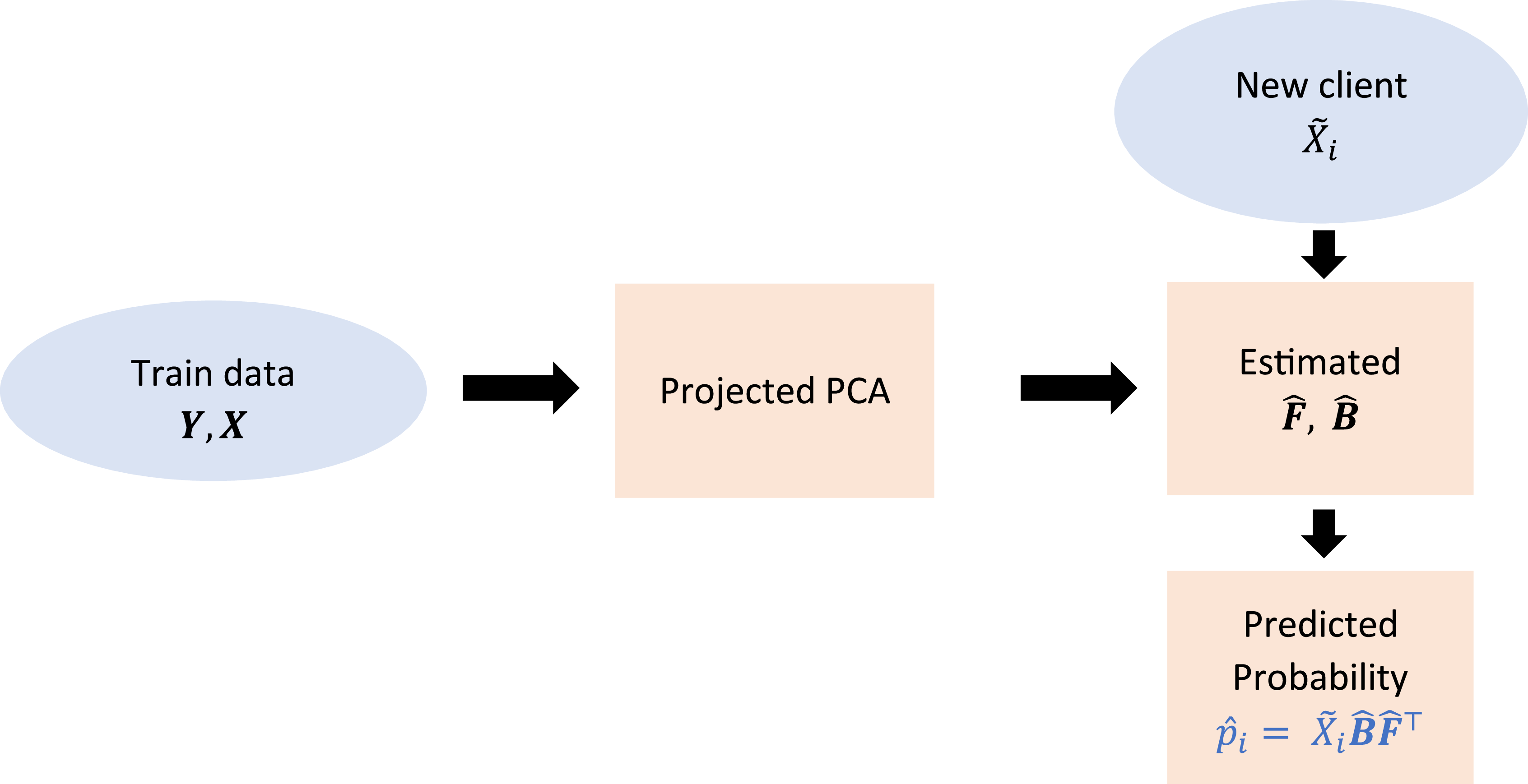
, thereby improving the estimation accuracy of the latent factors associated with customer characteristics. Once the parameters are estimated, the model predicts the probability of claim occurrence for each claim type, even for new customers whose characteristic information is available. Figure 1 illustrates the PPCA framework for predicting the probability of claim occurrence for new customers.
$\boldsymbol{Y}$
, thereby improving the estimation accuracy of the latent factors associated with customer characteristics. Once the parameters are estimated, the model predicts the probability of claim occurrence for each claim type, even for new customers whose characteristic information is available. Figure 1 illustrates the PPCA framework for predicting the probability of claim occurrence for new customers.
Overview of the PPCA framework.

In summary, the core idea of PPCA is to perform latent factor analysis on the projected matrix $\widehat {\boldsymbol{Y}}$
, derived by projecting
$\widehat {\boldsymbol{Y}}$
, derived by projecting $\boldsymbol{Y}$
onto the subspace spanned by
$\boldsymbol{Y}$
onto the subspace spanned by $\boldsymbol{X}$
. This projection reduces noise and facilitates estimation of the factor loading matrix
$\boldsymbol{X}$
. This projection reduces noise and facilitates estimation of the factor loading matrix $\boldsymbol{\varLambda} $
as a function of
$\boldsymbol{\varLambda} $
as a function of $\boldsymbol{X}$
. Furthermore, when PPCA is applied to profile customer risks across claim types, it naturally accounts for correlations among those types. Moreover, compared to approaches that fit separate models for each coverage type, PPCA addresses the overparameterization problem because it requires relatively fewer parameters for estimation. Specifically, the number of parameters required by the PPCA methodology,
$\boldsymbol{X}$
. Furthermore, when PPCA is applied to profile customer risks across claim types, it naturally accounts for correlations among those types. Moreover, compared to approaches that fit separate models for each coverage type, PPCA addresses the overparameterization problem because it requires relatively fewer parameters for estimation. Specifically, the number of parameters required by the PPCA methodology, $K \times \left( {D + m} \right)$
, is smaller than the number required by regression-based models,
$K \times \left( {D + m} \right)$
, is smaller than the number required by regression-based models, $\;D \times m$
(see Figure 2).
$\;D \times m$
(see Figure 2).
Graphical representation of the number of parameters for PPCA (left) and logistic regression (right).

An additional advantage of resolving the overparameterization problem is that it enables the model to capture nonlinear relationships between variables through the sieve estimation (Grenander, Reference Grenander1981; Geman and Hwang, Reference Geman and Hwang1982). The sieve estimation is an approximation method that models nonlinear relationships as series expansions, often using polynomial terms derived from a Taylor series. Specifically, in our empirical analysis, we apply a polynomial sieve to the continuous covariates by augmenting $X$
with polynomial terms up to degree
$X$
with polynomial terms up to degree $r$
. For each continuous covariate
$r$
. For each continuous covariate $x$
, we include
$x$
, we include $x,\;{x^2},{x^3}, \ldots ,{x^r}$
, so the covariate matrix becomes column-expanded, and we refer to
$x,\;{x^2},{x^3}, \ldots ,{x^r}$
, so the covariate matrix becomes column-expanded, and we refer to $r$
as the polynomial sieve order. Then, the fitted relationship can be nonlinear in the original covariates through higher-order terms such as
$r$
as the polynomial sieve order. Then, the fitted relationship can be nonlinear in the original covariates through higher-order terms such as ${x^2}$
and
${x^2}$
and ${x^3}$
. However, when dimensionality is high, the sieve estimation may improve the model’s ability to capture nonlinear relationships but also increase the risk of overfitting, which can degrade predictive performance. By contrast, resolving the overparameterization problem allows the model to incorporate nonlinear relationships without the drawbacks of overfitting.
${x^3}$
. However, when dimensionality is high, the sieve estimation may improve the model’s ability to capture nonlinear relationships but also increase the risk of overfitting, which can degrade predictive performance. By contrast, resolving the overparameterization problem allows the model to incorporate nonlinear relationships without the drawbacks of overfitting.
Figure 3 illustrates the average area under the receiver operating characteristic curve (AUC)Footnote 3 of the PPCA methodology as the polynomial order in sieve estimation increases, with the number of latent factors ranging from 10 to 20. The reported AUC values are obtained from 3-fold cross-validation using the customer features matrix. See Section 3 for details on the dataset. As shown in Figure 3, the performance of a logistic regression declines sharply with the inclusion of higher-order polynomial terms. In contrast, the out-of-sample AUC of PPCA drops sharply once the polynomial order exceeds five. This pattern may arise because higher-order polynomial expansions increase the number of parameters to be estimated, which exacerbates the overparameterization problem and can deteriorate out-of-sample performance. In contrast, PPCA can mitigate this issue by imposing a low-dimensional structure that limits the effective number of free parameters even when higher-order polynomial terms are included.
The average AUC of the PPCA model against the polynomial order in sieve estimation, varying the number of factors from 10 to 20. The dotted line represents logistic regression performance for comparison.

Although ensemble methods such as XGBoost (Chen and Guestrin, Reference Chen and Guestrin2016) often deliver superior predictive accuracy in binary classification tasks, they are limited primarily by the difficulty in interpreting the influence of individual customer characteristics on predicted probabilities. In contrast, the PPCA methodology provides interpretable coefficients that offer insights into the effects of customer characteristics on the probability of claim occurrence. A detailed discussion of the interpretation of these coefficients is presented in Section 4 and Appendix D.
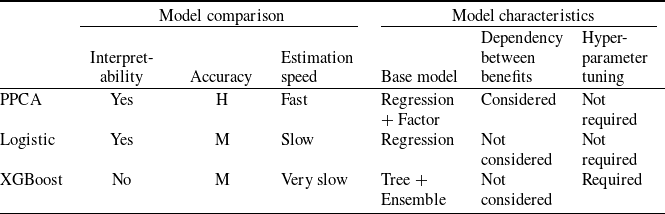
We clarify the difference between the proposed PPCA method and two other benchmarks with regard to performance and characteristics in Table 1. Logistic regression offers an interpretable linear framework but faces an overparameterization problem when the number of claim types is large, because it estimates separate logistic regressions for each claim type and thus entails $D \times m$
coefficients (see Figure 2), which may lead to overfitting. XGBoost, an ensemble tree-based model employing gradient boosting, effectively captures nonlinear relationships but requires careful regularization and can be computationally intensive. By contrast, PPCA is a latent factor model that mitigates overfitting while maintaining interpretability, provides a closed-form solution, and enables simultaneous parameter estimation across multiple claim types.
$D \times m$
coefficients (see Figure 2), which may lead to overfitting. XGBoost, an ensemble tree-based model employing gradient boosting, effectively captures nonlinear relationships but requires careful regularization and can be computationally intensive. By contrast, PPCA is a latent factor model that mitigates overfitting while maintaining interpretability, provides a closed-form solution, and enables simultaneous parameter estimation across multiple claim types.
Model comparison and characteristics.

Note: L, M, and H denote low, moderate, and high performance, respectively.
3. Data
The PPCA methodology employs two matrices: the customer characteristic matrix
X
and the customer-by-claim-type event matrix
Y
. The matrix
Y
is a binary matrix indicating whether a customer is indemnified for each specific claim type. We empirically design both $\boldsymbol{X}$
and
$\boldsymbol{X}$
and $\boldsymbol{Y}$
matrices from a large-scale life insurance dataset provided by a major life insurer in South Korea. The analysis spans two distinct periods: January 2017–December 2018 and January 2019–December 2021.Footnote
4
$\boldsymbol{Y}$
matrices from a large-scale life insurance dataset provided by a major life insurer in South Korea. The analysis spans two distinct periods: January 2017–December 2018 and January 2019–December 2021.Footnote
4
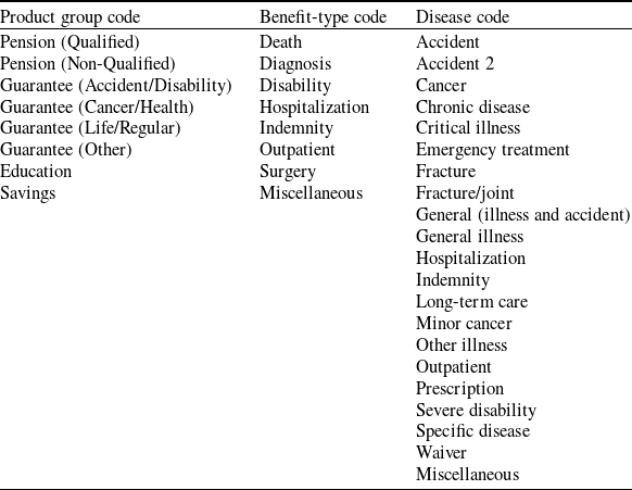
We include the claim classes by combining three categorical codes from the original dataset: product group, benefit-type classification, and disease classification. Each code comprises multiple distinct categories, as summarized in Table 2. Theoretically, these codes yield 1,344 potential combinations. However, not all combinations are observed in the data; hence, to ensure sufficient observations for estimation, we consider the combinations appearing at least 10 times during the analysis periods. This criterion yields 238 feasible claim classes, which form the columns of the customer-by-claim-type event matrix $\boldsymbol{Y}$
.
$\boldsymbol{Y}$
.
Classification codes for claim classes.

Note: Product group, benefit-type, and disease classification codes are used to construct the customer-by-claim-type event matrix.
The matrix $\boldsymbol{X}$
of customer characteristics contains various individual attributes, with each row representing a distinct customer and each column corresponding to an insured-specific feature. These features include numerical variables such as the customer’s age at policy inception and monthly household income, as well as categorical variables such as gender, residential type, and marital status.Footnote
5
Considering the predictive value of customers’ historical data on insurance-related behaviors, we included additional variables derived from this historical information. Specifically, “Claimed” variables indicate whether customers received insurance payments after policy inception within defined time frames – one, three, and five years – or at any time. Additionally, “Enrolled” variables were included to represent enrollment status across other product groups. After one-hot encoding, the customer characteristic matrix
$\boldsymbol{X}$
of customer characteristics contains various individual attributes, with each row representing a distinct customer and each column corresponding to an insured-specific feature. These features include numerical variables such as the customer’s age at policy inception and monthly household income, as well as categorical variables such as gender, residential type, and marital status.Footnote
5
Considering the predictive value of customers’ historical data on insurance-related behaviors, we included additional variables derived from this historical information. Specifically, “Claimed” variables indicate whether customers received insurance payments after policy inception within defined time frames – one, three, and five years – or at any time. Additionally, “Enrolled” variables were included to represent enrollment status across other product groups. After one-hot encoding, the customer characteristic matrix $X$
has
$X$
has $D = 77$
columns excluding sieve expansions, consisting of 65 customer attribute features, four “Claimed” variables, and eight “Enrolled” variables.
$D = 77$
columns excluding sieve expansions, consisting of 65 customer attribute features, four “Claimed” variables, and eight “Enrolled” variables.
Due to potential multicollinearity among the customer characteristics, we implement a variable selection procedure based on the partial-correlation interpretation of the inverse correlation matrix of the covariates. When there exist variable pairs with large partial correlations, matrix inversion can become numerically unstable and distort the resulting estimates. A heuristic clustering algorithm helps identify such variables by iteratively selecting subsets to minimize interdependence to avoid numerical instability during matrix inversion. This procedure mitigates multicollinearity while preserving the predictive performance of the model as much as possible.Footnote 6
4. Results
We first evaluate the performance of each model using the out-of-sample AUC estimated through 5-fold cross-validation. We implement the analysis separately for two distinct periods, where for each period, two scenarios were examined: one employing the entire dataset and the other for a stratified random sample comprising 5% of the dataset. We take into consideration the sampling scenario due to the computational intensity of the XGBoost method, which may result in impractically long estimation time for the complete dataset.
When we conduct the PPCA procedure, we implement a variable selection procedure due to potential multicollinearity among the customer characteristics. The procedure is based on the partial-correlation interpretation of the inverse correlation matrix of the covariates, as described in Section 3. To examine whether feature selection affects predictive performance, we compare the model performance with and without feature selection. Figure 4 compares the out-of-sample AUC of the PPCA model with feature selection and without feature selection across polynomial sieve orders and the number of latent factors. The horizontal dashed line indicates the average AUC from logistic regression with a polynomial sieve order of 1. Figure 4 shows that feature selection does not substantially affect predictive performance, while PPCA achieves a higher AUC than logistic regression across the factor specifications. We therefore use the selected feature set in all other analyses.
The average AUC of the PPCA model against the polynomial order in sieve estimation, with the number of factors varying from 10 to 22, with (left) and without (right) feature selection. The dotted line represents logistic regression performance for comparison.

Regarding the implementation of the XGBoost method, the absence of hyperparameter tuning typically results in suboptimal performance. However, given the extensive hyperparameter combinations with large-scale data, a comprehensive search on the entire dataset can be computationally intensive. In this regard, we use fixed hyperparameters to fit XGBoost to the full dataset. Instead, we consider the Bayesian optimization method for the 5%-sampled subset, where the Bayesian optimization helps evaluate 12 hyperparameter sets: two sets for initial exploration and ten selected through iterative Bayesian search.Footnote 7 For the PPCA method, we vary the number of latent factors from 10 to 22 to examine whether it exhibits overall outperformance relative to the two benchmark methods. Figure 5 shows the average AUC calculated across all claim classes and cross-validation folds, based on the full dataset for two subperiods. In each graph, the x-axis represents the polynomial order employed for sieve estimation to capture nonlinear relationships.Footnote 8
The average AUC across all claim classes and cross-validation folds against the sieve order for the models (without hyperparameter tuning for XGBoost), using the full sample from January 2017 to December 2018 (left) and from January 2019 to December 2021 (right).

We find in Figure 5 that PPCA achieved higher AUC values when the number of latent factors was between 10 and 14 across both periods, with the AUC tending to peak around sieve orders 3 and 2 in the first and second periods, respectively. Regarding the period-specific differences in the optimal number of latent factors and the sieve order, this may be because the latent dependence structure and the nonlinear relationship between $\boldsymbol{X}$
and the claim probability vary across periods. Regarding the non-monotone optimal number of latent factors and the sieve order, it may be because additional factors and higher-order sieve terms can reduce model misspecification error, but they also increase the number of parameters to be estimated and thus raise estimation error, which can offset improvements in out-of-sample AUC in finite samples.
$\boldsymbol{X}$
and the claim probability vary across periods. Regarding the non-monotone optimal number of latent factors and the sieve order, it may be because additional factors and higher-order sieve terms can reduce model misspecification error, but they also increase the number of parameters to be estimated and thus raise estimation error, which can offset improvements in out-of-sample AUC in finite samples.
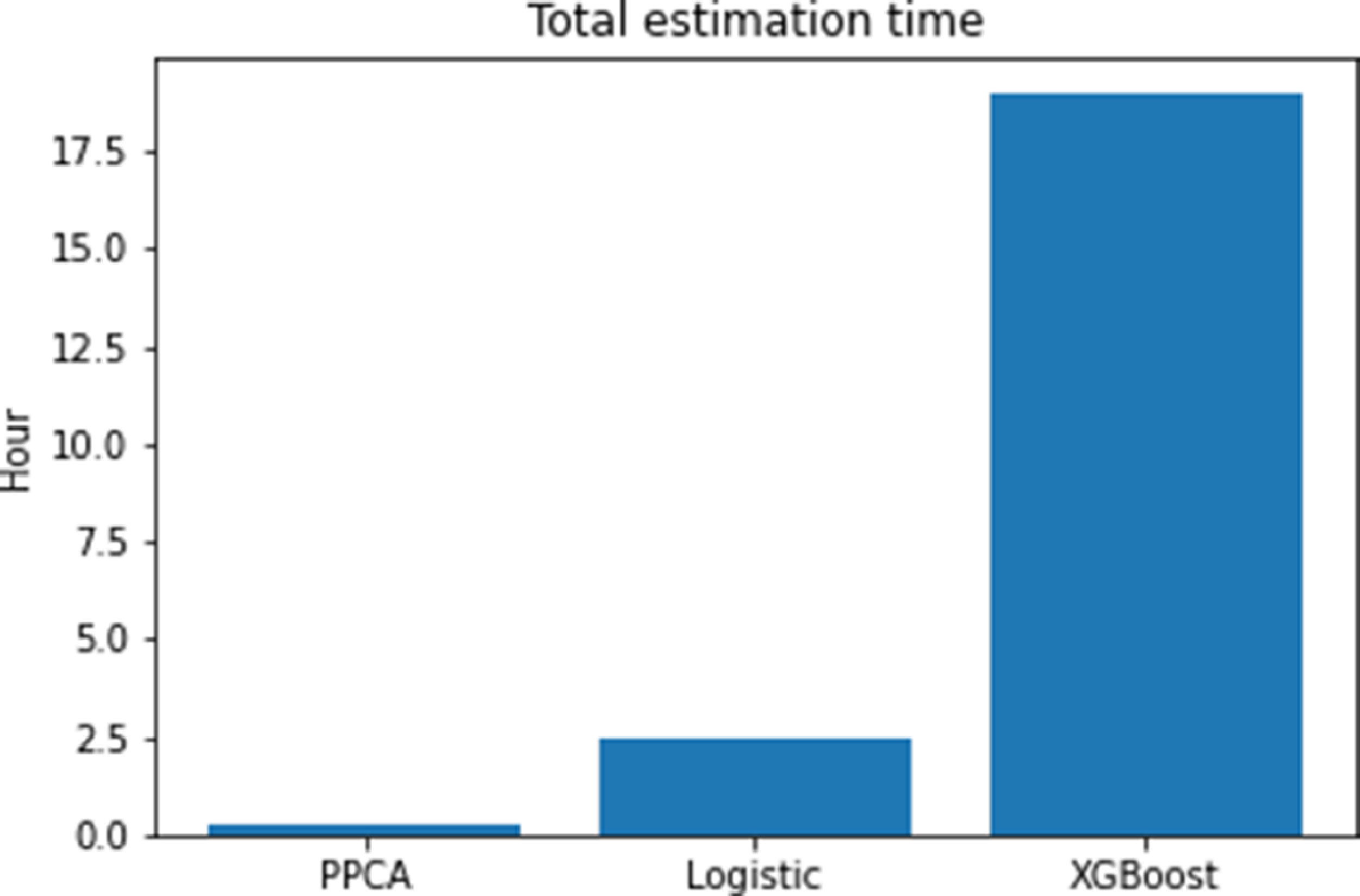
Furthermore, PPCA consistently outperformed logistic regression for most combinations of latent factor numbers and sieve orders. By contrast, XGBoost yielded the lowest AUC, likely due to the absence of hyperparameter tuning. Although decision tree-based methods such as XGBoost generally yield high performance with suitable regularization, employing a single set of hyperparameters for all claim types likely limited its performance. However, when it comes to the computational time, it turns out to be approximately 20 minutes for PPCA, 2 hours and 25 minutes for logistic regression, and around 19 hours for XGBoost to test the 5% sampled data from 2019 to 2021 (see Figure 6). This corresponds to a reduction in computational time of approximately 86% and 98% compared to logistic regression and XGBoost, respectively.
Comparison of total estimation time using 5% sampled data from 2019 to 2021 for PPCA, logistic regression, and XGBoost models.

We then check the model performance across product groups in Figures 7 and 8, where the average AUC across all cross-validation folds for each product group is displayed. The product groups that can be obtained from the dataset are eight categories (pension for qualified or unqualified, guaranteed life insurance for accident/injury, cancer/health, and whole/term life, education, and savings), which are in relatively high demand from the life insurer. We find that the optimal number of latent factors for the PPCA methodology varies among product groups. These findings suggest that overall predictive performance could be improved by grouping claim types with similar latent factors and applying the PPCA method separately.
The average AUC across all cross-validation folds against the sieve order for each category for PPCA, logistic regression, and XGBoost (without hyperparameter tuning) models, using the full sample from January 2017 to December 2018.

The average AUC across all cross-validation folds against the sieve order for each category for PPCA, logistic regression, and XGBoost (without hyperparameter tuning) models, using the full sample from January 2019 to December 2021.

Regarding the sieve order in the PPCA method, predictive performance does not demonstrate a consistent pattern across the two periods. This inconsistency implies that the nonlinear relationships between customer characteristics and the probability of claim occurrence may vary over time. In addition, we observe that out-of-sample AUC in the product-group analysis is more sensitive to the selected number of latent factors and the sieve order. This may be because restricting the analysis to claim types within each product group reduces the number of claim types $m$
, which provides less information across claim types for estimating the latent factor component
$m$
, which provides less information across claim types for estimating the latent factor component $\boldsymbol{F}$
and thus increases its estimation error.
$\boldsymbol{F}$
and thus increases its estimation error.
When comparing the performances of the methodologies, the PPCA outperforms the benchmark methods except for some product groups. Fluctuations in XGBoost relative performance across product groups may reflect its sensitivity to hyperparameter selection. A possible explanation for cases in which the PPCA underperforms logistic regression is that a product group may include claim types that do not share a common latent factor structure. That is, the PPCA is effective when claim types are accurately classified according to their shared latent factors. However, its performance may deteriorate if this classification is inadequate. This observation highlights the importance of correctly classifying claim types based on latent factor structures and separately applying the PPCA method to each group.
Figures 9–11 present the results of a 5% subsample case used for XGBoost hyperparameter tuning. Following hyperparameter tuning, XGBoost exhibits AUC values comparable to those of logistic regression in both periods. When evaluating the impact of sample size on predictive performance, we observe that overall AUC values decrease when using the 5% subsample compared to the full dataset, highlighting the importance of larger datasets for estimation accuracy.
The average AUC against the sieve order for the models using 5% sampled data (with hyperparameter tuning for XGBoost) from January 2017 to December 2018 (left) and from January 2019 to December 2021 (right).

The average AUC against the polynomial order for PPCA, logistic regression, and XGBoost (with hyperparameter tuning) across different product groups, using 5% sampled data from January 2017 to December 2018.

The average AUC against the polynomial order for PPCA, logistic regression, and XGBoost (with hyperparameter tuning) across different product groups, using 5% sampled data from January 2019 to December 2021.

In the left panel of Figure 9, which corresponds to the first period, the average AUC is uniformly lower at sieve orders 2 and 4. This may be because even-power terms are sign-invariant and thus discard directional information and primarily reflect magnitude. If the dominant nonlinear relationship is close to a monotone directional pattern in the first period, adding even-power terms may contribute little to reducing model misspecification error while still increasing complexity. This trade-off can be more pronounced with limited data.
For the second period, shown in the right panel of Figure 9 and consistent with Figure 5, the quadratic term may be enough to capture the main nonlinear component even in the 5% subsample, so the AUC peaks around sieve order 2 and then declines as higher sieve orders add complexity with limited incremental signal. In the cases of Figures 10 and 11, the analysis is conducted within each product group and additionally uses the 5% subsample, so both $m$
and the sample size
$m$
and the sample size $n$
are smaller. This can further increase estimation error. As a result, it can be harder to see patterns that are consistent with the full-sample results in Figures 7 and 8.
$n$
are smaller. This can further increase estimation error. As a result, it can be harder to see patterns that are consistent with the full-sample results in Figures 7 and 8.
Predicting the probability of claim occurrence is essential for effective decision-making in insurance practice. However, the practical utility of such predictions necessitates an understanding of how customer characteristics influence the estimated probabilities. Since the PPCA method is fundamentally based on a linear model, its results can be interpreted similarly to those of a linear regression model as follows:
 \begin{align}Y_{ij}=\mathop \sum \limits_{k=1}^{K} {\mathop \sum \limits_{d=1}^{D} X_{id}}{\widehat {B}_{dk}}{\widehat {F}_{jk}}+{\widehat {U}_{ij}}={\mathop \sum \limits_{d=1}^{D} X_{id}}{\widehat {\beta}_{dj}}+{\widehat {U}_{ij}},\end{align}
where ${\widehat \beta _{dj}} = \mathop \sum \nolimits_{k = 1}^K {\widehat B_{dk}}{\widehat F_{jk}}$
. We note that this representation also holds with sieve basis terms, since these terms simply expand the covariate vector
${\widehat \beta _{dj}} = \mathop \sum \nolimits_{k = 1}^K {\widehat B_{dk}}{\widehat F_{jk}}$
. We note that this representation also holds with sieve basis terms, since these terms simply expand the covariate vector ${X_i}$
and enter the model as additional covariates.
${X_i}$
and enter the model as additional covariates.
When customer features listed in Table B1 of Appendix B comprise binary and numerical variables, the coefficients can be directly interpreted as the impact of these features on the probability of claim occurrence. However, our empirical analysis includes nonbinary categorical variables such as customer region codes, as well as higher-order polynomial terms that capture nonlinearity in X . In such instances, interpreting the coefficients requires additional consideration.Footnote 9 We report coefficient estimates for variables exhibiting notable effects across product groups and periods in Appendix E.
5. Conclusion
Accurate estimation of the probability of claim occurrence is critical for insurers to effectively manage profitability and maintain solvency. In the era of large-scale data available from various sources, insurance customers’ risk profiles can be obtained at a granular level and used to achieve high estimation accuracy. In this regard, this study contributes to the literature by proposing a PPCA-based model to estimate the probability of claim occurrence across claim types using insured-specific characteristics. Our proposed approach is useful for analyzing what drives the probability of claim occurrence in an insurance portfolio, as it overcomes the overparameterization problem and captures correlations between claim types.
Using a large-scale insurance dataset from one of the largest Korean life insurers, we compare the proposed model with benchmark approaches (logistic regression and XGBoost) to demonstrate its ability to accurately predict the probability of claim occurrence. From the overall comparison of model performance, we find that our model generally outperforms the benchmark methods in terms of AUC. Our results also show that the proposed model is time-efficient, showing a reduction in computational time of approximately 86% and 98% compared to benchmark models (logistic regression and XGBoost, respectively). Our results provide insurers with practical insights to improve claims management efficiency and thus help maintain financial stability by accurately predicting the probability of claim occurrence.
Our conclusion demonstrates that the proposed framework with the PPCA effectively mitigates the overparameterization problem, showing its strong empirical performance over the competitors. However, although the sieve estimation enables the model to approximate nonlinear effects, it does not explicitly identify or optimize the polynomial order that best captures complex interactions among insured-specific characteristics. As a result, certain higher-order dependencies and interaction effects that shape an individual’s risk profile may remain partially unobserved.
In this regard, further studies could address the limitation by developing, for example, a data-driven criterion to determine the optimal order in sieve estimation or by integrating flexible nonlinear projection methods (such as kernelized or deep neural factor structures) into the PPCA framework. Moreover, applying the model to different insurance lines or longitudinal datasets could help evaluate its robustness over time and across contexts, offering a more comprehensive understanding of how customer characteristics interact to influence claim probabilities.
In our framework, the low-rank structure $\boldsymbol{\varLambda} {F^ \top }$
represents the Bernoulli probability matrix
$\boldsymbol{\varLambda} {F^ \top }$
represents the Bernoulli probability matrix $\boldsymbol{\Theta} = \left( {{\boldsymbol{\theta} _{ij}}} \right)$
for binary claim outcomes. While introducing a link function to model probabilities is a natural extension, an elementwise link does not resolve the overparameterization issue in high-dimensional settings. Addressing this challenge would require a matrix-wise link function tailored to projected PCA, which is technically demanding and beyond the scope of this paper. We leave this for future studies.
$\boldsymbol{\Theta} = \left( {{\boldsymbol{\theta} _{ij}}} \right)$
for binary claim outcomes. While introducing a link function to model probabilities is a natural extension, an elementwise link does not resolve the overparameterization issue in high-dimensional settings. Addressing this challenge would require a matrix-wise link function tailored to projected PCA, which is technically demanding and beyond the scope of this paper. We leave this for future studies.
Supplementary material
The supplementary material for this article can be found at https://doi.org/10.1017/asb.2026.10105
Funding statement
This work was partly supported by the Institute of Information & Communications Technology Planning & Evaluation (IITP)-Global Data-X Leader HRD program grant funded by the Korean government (MSIT) (IITP-2024-RS-2024-00441244) and by the National Research Foundation of Korea (NRF) grant funded by the Korean government (MSIT) (RS-2024-00343129) awarded to Kwangmin Jung, and by the Sogang University Research Grant of 2026 (202610002.01) awarded to Minseog Oh.








 Open access

