3.1. Climate conditions on Severnaya Zemlya

In general, the climate of SZ is typical for the High Arctic. The large-scale atmospheric circulation is dominated by the low-pressure area over the Barents Sea and Kara Sea and by the high-pressure areas over Siberia and the Arctic Ocean (Reference Bolshiyanov and MakeyevBolshiyanov and Makeev, 1995; Reference Alexandrov, Radinov and SvyashchennikovAlexandrov and others, 2000). During wintertime, anticyclone circulation connected with the Siberian and Arctic highs dominates, but cyclones coming from the Kara Sea reach the archipelago. In spring, the circulation shows winter characteristics, but with lower pressure gradients and cyclone activity. The summer is characterized by continually decreasing cyclone activity and the formation of a high-pressure area. In autumn, wintertime pressure fields start to develop and the cyclone activity increases to its annual maximum.

Meteorological measurements on SZ started only in 1930. Unfortunately, there are some data gaps in the 1930s and 1940s. Golomyanny station (Fig. 1; World Meteorological Organization (WMO) number 20087), located on a small island at the western tip of SZ (7 m a.s.l.), has an annual mean surface air temperature (SAT) of −14.7°C for the period 1951–80 (Reference Alexandrov, Radinov and SvyashchennikovAlexandrov and others, 2000). After a SAT maximum in the 1950s, Golomyanny data show a cooler period until 1980 and a warming trend since 1990, though without reaching the values of the 1950s (data from Reference PolyakovPolyakov and others, 2003b, http://www.frontier.iarc.uaf.edu/∼igor/research/data/airtemppres.php).

Annual mean precipitation is 186 mm at Golomyanny station (Reference Alexandrov, Radinov and SvyashchennikovAlexandrov and others, 2000), whereas the ice caps receive about 400 mm distributed throughout the year, with maxima in summer and autumn (Reference Bolshiyanov and MakeyevBolshiyanov and Makeev, 1995). According to the general circulation pattern, Reference Bolshiyanov and MakeyevBolshiyanov and Makeev (1995) demonstrated that the main part of precipitation on Vavilov ice cap occurs in connection with southerly and southwesterly winds, caused by north-eastward movement of moisture-bearing cyclones over the Kara Sea. The autumn precipitation maximum is connected to the increase in cyclonic activity: depressions causing much precipitation move from the North Atlantic. Cyclones, formed over northern Europe and western Siberia, are responsible for the summer precipitation maximum. An air-mass transport mainly from Asia, northern Eurasia, Europe and the Atlantic Ocean, as identified by trajectory analysis for spring (Reference Vinogradova and EgorovVinogradova and Egorov, 1996) and summer (Reference Vinogradova and PonomarevaVinogradova and Ponomareva, 1999), confirms these findings. We assume a similar pattern and origin of precipitation for the nearby AN ice cap, situated about 150 km north of Vavilov ice cap.

3.2. Drilling-site characterization and melting processes

Covering an area of 5575 km², the dome-shaped AN ice cap is the largest in the whole Russian Arctic, reaching a maximum elevation of about 750 m a.s.l. (Reference DowdeswellDowdeswell and others, 2002). To avoid a disturbed core stratigraphy, the drilling site was chosen in an area with flat subglacial topography and low horizontal ice-flow velocity (Reference FritzscheFritzsche and others, 2002). Although situated near the summit, the drilling site is located in the percolation zone and therefore, like almost all Arctic ice caps outside interior Greenland, is affected by infiltration of meltwater during summer. We assume that melting and infiltration processes occur in almost every summer due to temperatures above 0°C and/or high insolation.

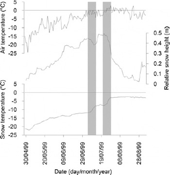
An automatic weather station (AWS) was run at the drilling site between May 1999 and May 2000, with a data gap of 2 months (during February and April 2000) due to a breakdown in power supply (Reference KuhnKuhn, 2000). The AWS data give the opportunity to characterize the temperature conditions near the drilling point for the 1999 summer season. Figure 2 illustrates daily mean values of air temperature (2.5 m above snow cover at the start in May 1999), snow height (calculated from the distance between sensor and snow cover, relative to the start) and snow temperature (0.5 m below snow cover at the start). Clearly visible are temperatures above 0°C in July and August, causing snowmelt and decrease of snow height. Strong increases in snow temperature within a few days, corresponding with decreasing snow height, indicate infiltration events. The meltwater pulses connected with latent-heat flow reach depths of 1 m (height difference between snow height and snow temperature logger) as a minimum, at least in fresh snow. At the end of August, almost all the snow that had fallen since May had sintered and melted, before new snow accumulation began. The maximum percolation depth on AN ice cap is uncertain. However, percolation deeper than two to three annual layers seems unlikely, since the ice layers, formed by refrozen meltwater, should be barriers to further infiltration. For the Lomonosovfonna ice core, extensive study by Reference PohjolaPohjola and others (2002a) showed that the infiltrated meltwater typically refreezes within the recent annual layer.

Fig. 2.

Data from an AWS near the drilling site for time period May–August 1999: air temperature (2.5 m above snow cover at the start in May 1999), relative snow height (relative to start in May 1999) and snow temperature (0.5 m below snow cover at start in May 1999). The horizontal black lines indicate 0°C. Grey shaded areas indicate infiltration events with decreasing snow height and increasing snow temperature.

The annual mean air temperature for May 1999–April 2000 was calculated as −15.7°C (Reference KuhnKuhn, 2000). Compared with the measured 10 m depth temperature of −10.2°C in April 2000, this indicates latent-heat flow of infiltrating meltwater, as mentioned above. From a comparison of AWS and Golomyanny SAT data, we calculated a mean temperature gradient of −0.5°C per 100 m altitude, with lowest values in summer and highest values in autumn as a result of sea-level freezing processes with release of latent heat.

6.1. Stable water-isotope ratios δ¹⁸O and δD

Due to their dependence on condensation temperatures, stable water-isotope ratios δ¹⁸O and δD in precipitation are commonly accepted as valuable proxy for local- to regional-scale temperatures in high polar latitudes. For the AN ice core, the relationship between all δ¹⁸O and δD values in the presented core section is δD = 7.46δ¹⁸O − 0.11 (R ² = 0.98, n = 2248; Fig. 4). Considering only the annual mean values, derived by averaging all isotope values between the defined annual marks, the isotopic relationship is calculated as δD = 7.55δ¹⁸O + 1.84 (R ² = 0.99, n = 116; Fig. 4). Both relationships are close together and can be interpreted as a local meteoric waterline (LMWL). Additionally, they differ only slightly from the global meteoric waterline (GMWL), which is defined theoretically as δD = 8δ¹⁸O + 10 (Reference CraigCraig, 1961) and calculated on a global scale as δD = 8.17δ¹⁸O + 10.35 (Reference Rozanski, Araguás-Araguás, Gonfiantini, Swart, Lohmann, McKenzie and SavinRozanski and others, 1993). From this, it follows that the mean isotopic composition of the AN ice core is not affected by considerable changes owing to evaporation. Therefore, the AN ice-core stable-isotope data seem to be suitable for palaeoclimate studies. Statistical descriptions of the stable water-isotope data (single values and annual mean values) are given in Table 1.

Table 1.

Statistical descriptions of AN ice-core stable water-isotope data

For palaeoclimatic consideration of stable-isotope data, we focused on δ¹⁸O, which is more common in Arctic ice-core studies and therefore suitable for comparisons. To evaluate the palaeoclimatic significance of AN δ¹⁸O data, we compared them with instrumental as well as composited SAT time series and other ice-core data. For the calculation of correlation coefficients the time series were detrended by removing the linear trends. We used annual mean values and 5 year running mean (5yrm) values of AN δ¹⁸O and SAT data, since the effects of melting, infiltration and refreezing processes on the stable-isotope data should be reduced or even negligible when smoothing the dataset over 5 years.

We did not find any good agreement between AN δ¹⁸O data and SAT time series from the nearest meteorological station, Golomyanny (r _5yrm = 0.27; data from Reference PolyakovPolyakov and others, 2003b). Since Golomyanny is situated on a small island only 7 m a.s.l., we assume that its SAT is controlled mainly by the local occurrence of sea ice, especially in the summer and autumn seasons. It therefore represents a very local climate. In contrast, temperature conditions at the AN ice-cap summit, as well as at the precipitation condensation level, are relatively independent of the local sea-ice occurrence at Golomyanny.

Since there are no Central Russian Arctic SAT time series reaching back to the 19th century, we chose additional stations, mainly from the Atlantic and Eurasian sub-Arctic, with respect to their spatial vicinity on the one hand and temporal extension of the time series on the other. We present the correlations for some of these SAT time series in Table 2. The best accordance between AN δ¹⁸O and instrumental SAT time series (1883–1998) was found for Vardø (r _5yrm = 0.62) and Arkhangelsk (r _5yrm = 0.61) stations, located at the Barents Sea and White Sea coasts, respectively (Fig. 5; data from Climatic Research Unit (CRU), Norwich, UK; Reference Brohan, Kennedy, Harris, Tett and JonesBrohan and others, 2006). Compared with Golomyanny, their SATs are not (or in the case of Arkhangelsk to a much lesser extent) influenced by the occurrence of sea ice. The good correlations and similarities of the time series reveal again the influence of the Atlantic Ocean via the Barents Sea and Kara Sea on SZ region SAT conditions. Additionally, we found a strong correlation (r _5yrm = 0.72; Fig. 5) with the composite Arctic (north of 62° N) SAT anomalies time series of Reference PolyakovPolyakov and others (2003b). However, one should note that these strong correlations are mainly due to common multi-annual variability (Table 2).

Table 2.

Correlation coefficients between the detrended time series of AN δ¹⁸O and of selected sub-Arctic and Arctic SAT (r _y for annual mean values, r _5yrm for 5 year running mean values) in the given time periods. The reduced degrees of freedom due to autocorrelation were taken into account for the calculation of the levels of significance. The WMO stations are sorted from east to west (see Fig. 1)

The strong correlations to instrumental and composite SAT data show that AN δ¹⁸O data are representative for SAT changes, not only for the central Russian Arctic, but also for the western and possibly whole Eurasian Arctic and sub-Arctic. Since there are no meteorological data from the central Russian Arctic and only a few time series in the Eurasian Arctic spanning more than 100 years, our high-resolution AN δ¹⁸O data are very valuable for further palaeoclimatic studies in the Eurasian Arctic.

The AN δ¹⁸O time series shows a distinct increasing trend with pronounced changes since 1883. Starting from a low level of about −22‰, δ¹⁸O values increased to values of −18‰ at about 1920 and 1940. From 1950 to the 1980s they oscillated about −20‰ and rose again afterwards. Besides the strong warming in the first two decades of the 20th century the most prominent feature of the AN δ¹⁸O time series is the double-peaked SAT maximum between 1920 and 1940. These values were not reached again until the end of our record in the 1990s. This agrees with the instrumental sub-Arctic and Arctic SAT data (Fig. 5). The double-peak structure of this SAT maximum seems to be a specific feature of the Eurasian Arctic, since the 1920 peak is not visible in other SAT time series (e.g. Bodø or Akureyri). Based on instrumental data, Reference PrzybylakPrzybylak (2007) stated that for the whole Arctic the decade 1936–45 and the year 1938 were the warmest in the 20th century. Only the period 1995–2005 and the year 2005, respectively, reached and exceeded these values. This SAT pattern shows the Arctic peculiarity compared with the whole Northern Hemisphere (NH), where the SAT maximum values at about 1940 have been exceeded since the end of the 1980s (Fig. 5; data: http://data.giss.nasa.gov/gistemp/tabledata/NH.Ts.txt).

AN δ¹⁸O data show distinct similarities to the ice-core δ¹⁸O time series from Austfonna ice cap, Svalbard, (Reference IsakssonIsaksson and others, 2005) and Vetreniy ice cap, FJL, (Reference HendersonHenderson, 2002) whereas the accordance to Lomonosovfonna (Reference IsakssonIsaksson and others, 2005) is not as good. AN, Austfonna (750 m a.s.l.) and Vetreniy (500 m a.s.l.) ice caps are located at relatively low altitudes and are therefore more sensitive to SAT changes. In contrast, glaciers of higher elevation like Lomonosovfonna (1250 m a.s.l.) seem to reflect primarily free atmospheric climate signals (Reference IsakssonIsaksson and others, 2005). The higher sensitivity of the lower-altitude ice caps is also visible in the broader range of δ¹⁸O values (about 4‰ for AN and Austfonna for 5yrm in the 20th century) compared with Lomonosovfonna (about 2‰). The range differences may also be influenced by different impacts of sea ice and of the dampening North Atlantic, as well as by the more frequent temperature inversions at the lower altitudes as reported for Austfonna compared with Lomonosovfonna (Reference IsakssonIsaksson and others, 2005).

In contrast to these Eurasian Arctic ice-core data, the accordance between AN δ¹⁸O data and the often used proxy-deduced SAT time series of Reference OverpeckOverpeck and others (1997) is less pronounced (Fig. 5). This is probably caused by the predominance of Canadian and Alaskan Arctic proxy sites in this composite record, whereas just a few proxy records of the Eurasian Arctic are considered.

6.2. Deuterium excess

The second-order parameter deuterium excess d (Reference DansgaardDansgaard, 1964) in precipitation depends largely on the evaporation conditions in the moisture source region, to a lesser degree on condensation temperatures but also on secondary kinetic fractionation processes. The main controlling factors are the relative air humidity and the sea-surface temperature (SST) and, to a lesser extent, wind speed during evaporation (Reference Rozanski, Araguás-Araguás, Gonfiantini, Swart, Lohmann, McKenzie and SavinRozanski and others, 1993). Assuming no significant changes in the spatial distribution of the moisture source regions, variations of d can be interpreted in terms of changing SST and relative humidity conditions (e.g. Reference Hoffmann, Jouzel and JohnsenHoffmann and others, 2001).

The mean d values of the considered core section account for 10.7‰ for all single samples and 10.8‰ for the annual mean values, respectively (Table 1). These values are typical for precipitation in high-latitude coastal areas (Reference Johnsen, Dansgaard and WhiteJohnsen and others, 1989). Therefore, we assume an oceanic main moisture source, whereas substantial water recycling from the continents seems unlikely. However, the AN mean d value is slightly higher than the 9.5‰ for the period 1883–1990 in the Lomonosovfonna ice core (Reference DivineDivine and others, 2008), the only Arctic ice core outside of Greenland for which a study of d was performed so far. This points to different moisture generation and transport regimes, probably due to the more remote location of SZ compared with the much more Atlantic-influenced western Svalbard.

In general, high (low) d values are caused by high (low) SST as well as by low (high) relative humidity during evaporation (Reference Johnsen, Dansgaard and WhiteJohnsen and others, 1989). However, on seasonal timescales d seems to be controlled mainly by the relative humidity. In the AN d record, high (low) d values in winter (summer) are connected with lower (higher) relative humidity in the moisture source region, outbalancing lower (higher) SSTs during that time. This pattern of opposite behaviour of δ¹⁸O and d corresponds with the isotopic data of the Global Network of Isotopes in Precipitation (e.g. Reference Rozanski, Araguás-Araguás, Gonfiantini, Swart, Lohmann, McKenzie and SavinRozanski and others, 1993) and model calculations (Reference Fröhlich, Gibson and AggarwalFröhlich and others, 2002).

Based on the assumption of nearly constant annual mean values of relative humidity in the moisture source region, multi-annual variations of d should be related mainly to SST changes (Reference Hoffmann, Jouzel and JohnsenHoffmann and others, 2001). The AN d time series shows a distinct decreasing trend over the 115 years considered. This is a reverse picture compared with δ¹⁸O (Fig. 6), corresponding with the findings in the seasonal cycles of d and δ¹⁸O. Only the strong δ¹⁸O peak about 1920 shows no counterpart in d (see below). The highest d values (about 12‰) occurred about 1900 and the lowest (about 9‰) in the 1990s. A similar decreasing trend is visible in the ice cores from central Greenland (Reference Hoffmann, Jouzel and JohnsenHoffmann and others, 2001), but not in the Lomonosovfonna ice core (Reference DivineDivine and others, 2008), where an increasing d trend is visible for the period considered here.

Fig. 6.

Time series of AN δ¹⁸O, AN d, Kara Sea August sea-ice anomalies (Reference PolyakovPolyakov and others, 2003a, computed against mean of the entire period) and North Atlantic SST anomalies (Reference Gray, Graumlich, Betancourt and PedersonGray and others, 2004). The thin grey lines indicate annual mean values; the thick black lines show 5yrm.

The main feature of the AN d time series is the strong decrease since 1970, also detectable in the ice-core records from central Greenland (Reference Hoffmann, Jouzel and JohnsenHoffmann and others, 2001), but not in the Lomonosovfonna ice core, which shows an increase (Reference DivineDivine and others, 2008). Assuming the positive d–SST relationship both the general decreasing trend and the strong d decrease after 1970 in the AN d record would indicate corresponding SST decreases in the main moisture source region. However, no comparable cooling trends are visible in the SST time series of the North Atlantic (0–70° N) (Reference Gray, Graumlich, Betancourt and PedersonGray and others, 2004; data: ftp://ftp.ncdc.noaa.gov/pub/data/paleo/treering/reconstructions/amo-gray2004.txt), which is the supposed main moisture source for precipitation reaching AN ice cap (Fig. 6), as well as in the NH SAT record (Fig. 5). Opposed to the AN d record, the North Atlantic SST has increased strongly since 1970. Such an opposite behaviour is also detectable about 1940, where a distinct d minimum was accompanied by high SST values. This pattern indicates that in hemispherical warmer periods (e.g. about 1940 and since 1970; Fig. 5) AN ice cap receives more precipitation from moisture evaporated at lower SSTs, for example due to a northward shift of the moisture source or a significant moisture contribution of a secondary regional source (Reference Johnsen, Dansgaard and WhiteJohnsen and others, 1989). Since most precipitation on SZ is caused by air masses moving from the south and southwest, the Kara Sea could be a regional moisture source (Fig. 1) with its sea-ice cover as the main controlling factor for summer and autumn evaporation. The time series of Kara Sea August sea-ice extent anomalies (Reference PolyakovPolyakov and others, 2003a; data: http://www.frontier.iarc.uaf.edu/∼igor/research/ice/icedata.php) shows a pattern similar to AN d data (r _5yrm = 0.51 for detrended data, p = 0.05; Fig. 6). A low sea-ice extent in the Kara Sea allows higher evaporation rates and leads to higher contribution of regional moisture to AN ice-cap precipitation. This results in lower d values due to the lower SST of the Kara Sea compared with the North Atlantic. In contrast, high sea-ice extent prevents a considerable regional moisture contribution, preserving the initially higher d values. The missing d counterpart of the 1920 δ¹⁸O peak can also be explained with this approach. The first part of the strong early 20th-century warming about 1920 occurred primarily in the winter season (Reference PolyakovPolyakov and others, 2003b). This did not lead to a substantial decrease in sea-ice extent in the Kara Sea and therefore not to a considerable regional moisture contribution and a decrease of d values. Since 1930 a warming of the non-winter season is perceptible, causing the absolute SAT maximum about 1938 (Reference PolyakovPolyakov and others, 2003b). This resulted in a corresponding decrease of sea-ice extent, leading to an amplified regional evaporation and, thus, a minimum in d.

Therefore, we assume the Kara Sea to be an important secondary moisture source region for the air masses reaching SZ, as well as the AN deuterium excess to be an indicator of temperature changes in the surrounding seas and the connected sea-ice extent changes. However, this is not the case for the d record of the Lomonosovfonna ice core, which can be interpreted as a proxy for the SST variability of the mid-latitude western North Atlantic (Reference DivineDivine and others, 2008).

6.3. Melt-layer content

The amount of melt layers in ice cores is a proxy for the summer warmth at the ice-cap surface (Reference KoernerKoerner, 1977). We calculated the melt-layer content by the proportion of melt-layer ice per metre by weight. As melt layer we considered ice, which consists of firn, infiltrated by a visible content of meltwater, independent of the amount of meltwater. Summertime meltwater infiltration on AN ice cap is irregular, as shown by Reference FritzscheFritzsche and others (2005). Percolation deeper than the corresponding annual layer leading to the formation of superimposed melt features may occur, at least in the warmest summers (section 3.2). Consequently, as a nearly annual resolution is not possible, we identified the melt-layer content per metre.

The melt-layer content in the AN ice core shows a strong increase at about the beginning of the 20th century, remains on a high level until about 1970, despite distinct variations, and exhibits a strong decrease in the most recent decades (Fig. 5). The ice cores from Vetreniy ice cap (Reference HendersonHenderson, 2002) and Austfonna ice cap (Reference WatanabeWatanabe and other, 2001) show similar melt-layer records, in contrast to the Lomonosovfonna melt-layer time series (Reference KekonenKekonen and others, 2005).

Whereas the first increase in the AN melt-layer record is also perceptible in a rise in the δ¹⁸O time series, there are distinct differences between both proxies later on. Around the δ¹⁸O-derived SAT maxima at about 1920 and 1940, as well as in the last decades, the melt-layer content shows sharp declines, whereas it exhibits higher values in the cooler 1950s and 1960s, indicating different seasonal temperature trends. For example, the strong warmings at about 1920 and 1940 occurred primarily in winter and autumn, which is supported by the studies of Polyakov and others (Reference Polyakov2003b; see above) and of Reference HendersonHenderson (2002) for the Vetreniy ice core. We did not find any correspondence between the melt-layer content and the Golomyanny summer SAT record (not shown here), which is influenced mainly by the cold Kara Sea due to melting sea ice. However, we assume that the melt-layer content in the AN ice core reflects predominantly the local summer conditions at the ice-cap surface, determined not only by the temperature, but also by the energy balance. Hence the significance of the melt-layer content in terms of regional SAT conditions is limited, at least on such short timescales as considered here.

6.4. Major ions

The ion record of ice cores reflects the atmospheric aerosol concentrations (e.g. Reference Legrand and MayewskiLegrand and Mayewski, 1997). However, ions deposited in glaciers with percolation are subject to post-depositional changes (Reference KoernerKoerner, 1997). The initially deposited AN chemical profile is superimposed by melting, infiltration and refreezing processes. Reference Weiler, Fischer, Fritzsche, Ruth, Wilhelms and MillerWeiler and others (2005) found that the AN ion record does not reflect seasonal atmospheric changes, but can be considered as an annually varying melting/refreezing signal. Most years seem to be represented by a peak of the more conservative ions such as sodium, which was used to achieve a depth–age scale (Reference Weiler, Fischer, Fritzsche, Ruth, Wilhelms and MillerWeiler and others, 2005; see also section 5). However, using mean values (here: 5yrm values) seems to be promising to detect lower-resolution changes in ice-core chemistry. In this subsection, we focus on 20th-century trends in AN ion data and two singular events, which are assumed to be of volcanic origin (see below).

The sea-salt ions sodium and chloride increased from a relatively low level at about 1900 to maximum values between 1910 and 1925 (Fig. 7). From this time the sea-salt ions show a decreasing trend. In the most recent years, values comparable to those at about 1900 were reached. Nevertheless, until about 1970 they remained on a high level characterized by a high-frequency variability. The period 1900–70 is characterized by the highest melt-layer content in the core section shown here. Therefore, the high variability could be caused or strengthened by meltwater percolation due to accumulation of leached ions in or above a melt layer. This assumption is supported by similar variations of the other ions of sea-salt origin: magnesium, calcium and (not shown here) potassium.

Fig. 7.

Time series of AN δ¹⁸O, AN melt-layer content, AN major ions and magnesium to sodium ratio by weight. The thin grey lines indicate annual mean values; the thick black lines indicate 5yrm (for AN melt-layer content 1 and 3 m running mean values, respectively). The dashed lines as well as numbers in parentheses represent non-sea-salt values. The horizontal black line indicates the magnesium to sodium ratio of sea water.

Similar records of sea-salt ions with a mid-20th-century maximum and a distinct decrease thereafter are also found in the Vetreniy ice core (Reference HendersonHenderson, 2002), in the Austfonna ice core (Reference WatanabeWatanabe and others, 2001) with maximum values for 1920–63 and, less pronounced, in the Lomonosovfonna ice core (Reference IsakssonIsaksson and others, 2001; Reference KekonenKekonen and others, 2005). Reference KekonenKekonen and others (2005) attributed this decrease to a substantial loss of ions due to increased melting and runoff, whereas Reference IsakssonIsaksson and others (2001) stated a decreasing deposition.

The magnesium to sodium ratio, introduced as a sensitive indicator for meltwater percolation in the Austfonna ice core by Reference Iizuka, Igarashi, Kamiyama, Motoyama and WatanabeIizuka and others (2002), shows no long-lasting decrease (Fig. 7). Only three short-term drops about 1920, 1930 and 1950 are detectable, accompanied by increased values in the years before. This indicates short phases of preferential elution of magnesium with respect to sodium and accumulation in deeper layers. However, no decline of this ratio in the last few decades is perceptible, corresponding to the decrease in sea-salt ion concentration. Additionally, the melt-layer content shows the lowest values of the 20th century for this period, indicating that an increased loss of ions owing to increased melting and runoff seems unlikely. Hence the decreasing sea-salt ion trend favours a decreasing deposition due to lower wind speed, a change of dominating air masses or storm tracks. Since the Svalbard and FJL ice cores show similar patterns, the reasons for this decrease seem not to be only regional, but on a larger scale, covering at least parts of the Eurasian Arctic. However, a possible further growth of AN ice cap with a subsequent rise in altitude due to higher values of mean annual layer thickness since 1935 (see section 5) could also have contributed.

Short-term peaks in ice-core ion time series are often caused by major volcanic eruptions. During these eruptions large amounts of aerosols are injected into the atmosphere, leading to increased ion concentrations, particularly of sulphate (e.g. Reference Legrand and MayewskiLegrand and Mayewski, 1997). In the AN sulphate record, two outstanding sharp peaks are visible, ascribed to the years 1956 and 1912 by δ¹⁸O cycle counting (Fig. 7). These values represent the highest values of sulphate concentrations for at least the last 1500 years, and of electrical conductivity in the whole AN ice core. The peaks were interpreted as imprints of the large volcanic eruptions of Bezymianny in 1956 and Katmai in 1912 and were therefore used as reference horizons for our age model. It is notable that for both events not only sulphate increased significantly, but all ions show enlarged values (Fig. 7). In both cases the magnesium to sodium ratio shows smaller declines in the layers directly above the peaks (Fig. 7), indicating leaching of ions. Therefore, it is likely that these peaks were amplified by infiltration processes and accumulation of ions. However, the peak linked to the Bezymianny eruption was identified clearly as of volcanic origin by Reference Weiler, Fischer, Fritzsche, Ruth, Wilhelms and MillerWeiler and others (2005), whereas this was not necessarily the case for the 1912 peak. The Bezymianny eruption was also detected in the Lomonosovfonna ice-core sulphate record, whereas there was no hint for the Katmai-related peak (Reference IsakssonIsaksson and others, 2001; Reference KekonenKekonen and others, 2005). However, there are spikes in the Austfonna sulphate profile (fig. 6 in Reference Iizuka, Igarashi, Kamiyama, Motoyama and WatanabeIizuka and others, 2002) which could be related to the two peaks in the AN ice core. Also, in the ice core from Vetreniy ice cap, a strong peak in sulphate is perceptible about 1956 (Reference HendersonHenderson 2002), even though not attributed to the Bezymianny eruption.

The concentrations of nitrate and sulphate in the AN ice core show a distinct anthropogenic imprint with a strong increase in the 1960s, maximum values about 1970 and decreasing values thereafter. This pattern corresponds to the records of the Svalbard and FJL ice cores (Reference IsakssonIsaksson and others, 2001; Reference WatanabeWatanabe and others, 2001; Reference HendersonHenderson, 2002; Reference KekonenKekonen and others, 2005) and was attributed to regional industrial sources by Reference Weiler, Fischer, Fritzsche, Ruth, Wilhelms and MillerWeiler and others (2005), who discussed these records in detail, even though with the slightly different age model mentioned above.