

Introduction
Glacial flow is driven by gravity and is restrained by forces acting at the bed or sides or by forces transmitted along the flow line. The relative role of these restraining forces is not generally clear, but how they act together has a central effect on the resulting shape and velocity of the glacier. This has been a long-standing problem in glaciology, and earlier authors have sought ways to combine the resistive stresses so that strain-rates can be simply calculated.
In the present work, the methods developed in the companion papers Reference Van deer Veen and Whillans(Van der Veen and Whillans, 1989a, Reference Van deer Veen and Whillansb; hereafter referred to as part I and part II) are applied to calculate the three-dimensional stress and velocity distribution. The surface effects of stress variations are measured on a glacier and the causative stresses at depth are calculated from these data. The velocities at depth are also so obtained. Field data are thus used to determine where resistive stresses are large or small, and to obtain values for the associated velocities.
There is an inherent limitation to the valid resolution that can be obtained from an inverse calculation of the sort used here. A general glacier has stress and velocity variations at all scales near the bed but short-scale variations are not exhibited at the upper surface. This is because the glacier acts as a filter and averages the shorter-scale features while transmitting them to the surface. If the constitutive relation is non-linear, so too is this averaging. Thus, starting with measured surface effects as is done here, it is not possible to obtain meaningful stress or velocity variations at depth at a horizontal scale of less than the scale of the effects at the surface.
This issue proved to be the main challenge with the application of this method. There is nothing in the equations developed for this method to prohibit the calculation of short-scale variations at depth, and, unless precautions are taken, small changes in input data produce very different calculated deep-stress and velocity variations. The simplest solution is not to allow short-scale variations by smoothing the velocity field at selected depths as the calculation proceeds downward. This is done here using Gaussian smoothing.
The method is applied to Byrd Glacier, an outlet glacier that links the East Antarctic inland ice and the Ross Ice Shelf (Fig. 1). It has a full set of surf ace-velocity and elevation data and so is suitable for this kind of analysis. For this glacier, 471 velocities and elevations have been obtained photogrammetrically (Reference BrecherBrecher, 1986), which is about one per 6 km2, and the data are distributed nearly uniformly over the studied section.

Fig. 1. Part of Antarctica: Byrd Glacier drains the East Antarctic ice sheet and flows into the Ross Ice Shelf.
This contribution is organized in the order of computation. It begins with the use of measured surface velocities to compute resistive stress at the surface. Data on thickness and surface slope are then described and used to compute driving stress. First, calculations are done for the simple and somewhat unrealistic case of strain-rates being constant with depth and thickness being constant across the width of the glacier. This case has the merit of simplicity in calculation. Then the simplifications are relaxed and the stresses and strain-rates at depth are calculated according to the method described in the second part of part I. The results of both the simple and the full calculation are maps of basal drag over the stretch of studied glacier.
Velocities
Surface velocities are from Brecher (personal communication, 1986) and are gridded in a manner only slightly different from that in Reference BrecherBrecher (1986). Brecher’s coordinate system is used, in which the x-axis is horizontal and mainly down-glacier, and the y-axis is perpendicular and anti-clockwise to it in map view. The origin of the x-axis is close to the site of flotation on sea-water as detected by an abrupt change in radio-echo strength from the bed. The grids of the x- and y-components of velocity are constrained to reach nearly zero values at the lateral margins and are smoothed consistent with measurement uncertainties. In order that the gridded velocity passes through zero at the margins, zero velocity data at the lateral margins are provided to the gridding software (called SURFACE II) as well as up-glacially directed longitudinal velocity “data” outside the glacier. This procedure may not be necessary with other gridding software. After gridding to a mesh spacing of 625 m, binomial smoothing with a standard deviation of 2 km is applied. The standard deviation obtained from the difference between the measured and gridded values for the x-component of velocity as shown in Figure 2a is 69 m a−1. This exceeds measurement error (which has a standard deviation of 27 m a−1), but the discrepancies are largest close to the lateral margins. For that reason, the calculated results near the boundaries are unreliable and are omitted on subsequent maps. The y-component of velocity differs from the data with a standard deviation of only 13 m a−1, and this is fully satisfactory.

Fig. 2. Gridded velocities and velocity components at the surface. Flow is left to right and the glacier begins to float at about x = 0: (a) x-component of velocity, ux; (b) y-component of velocity, uy, positive for flow towards the top of the figure; (c) longitudinal stretching, ![]() (d) lateral spreading,
(d) lateral spreading, ![]() Contour interval for velocities is 50 m a−1 and for velocity gradients is 0.005 a−1.
Contour interval for velocities is 50 m a−1 and for velocity gradients is 0.005 a−1.
Using the gridded and smoothed velocities, the velocity gradients and strain-rates (Figs 2c, d, 3a-c) are readily calculated. Within the main part of the glacier, longitudinal stretching, ∂u
x
/∂x (Fig. 2c), shows larger gradients for the grounded part than where the glacier is afloat. The variation in the grounded part has a longitudinal wavelength of about 13 km. Lateral spreading, ∂u
y
/∂y (Fig. 2d) shows a similar contrast between grounded and floating parts. Of special interest is the neighboring high and low near x = −13 km. Side shear, ∂u
x
/∂
y
(Fig. 3a), is concentrated at the margins where afloat but shows effects across the full width of the glacier where grounded. Flow-line turning, ∂u
y
/∂x (Fig. 3b), is relatively simple except for the right-left-right “snaking” action in the upper part of the grounded part. Shear strain-rate, ![]() (Fig. 3c), is derived from the data in Figures 3a and b.
(Fig. 3c), is derived from the data in Figures 3a and b.

Fig. 3. Further velocity gradients at the surface: (a) lateral shear, ∂u
x
/∂y; (b) turning of flow, ∂u
y
/∂x; (c) shear strain-rate, ![]() ; (d) effective strain-rate,
; (d) effective strain-rate, ![]() . Contour interval is 0.005 a−1.
. Contour interval is 0.005 a−1.
Of special interest is the effective strain-rate, ![]() (Fig- 3d),
(Fig- 3d),

in which the strain-rate is defined as:

for xx
≡ x, xy
, ≡ xz ≡ z The effective strain-rate describes the overall level of deformation rate and is ten times larger near the margin than in the center. This means that there is important stress softening at the margins. The variation along the center is due mainly to the vertical strain-rate, ![]() and secondarily to the “snaking” in the flow-line turning, ∂uy/∂x. However, to a first approximation, the effective strain-rate shows that strain-rate and stress levels are large near the margins and less in the center.
and secondarily to the “snaking” in the flow-line turning, ∂uy/∂x. However, to a first approximation, the effective strain-rate shows that strain-rate and stress levels are large near the margins and less in the center.
Resistive Stresses at the Surface
The strain-rates are used to calculate deviatoric and then resistive stresses. Deviatoric stresses, σ′ ij follow from the flow law:

in which the exponent, n, is initially taken as equal to 3 and the stiffness parameter is 700 kPa a1/3 at −25°C (Reference HookeHooke, 1981). It is, however, the resistive stresses, Rij , that most simply apply to force balance and these follow from the equivalencies in part I:
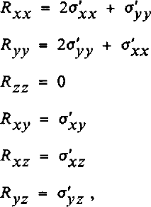
in which bridging effects have been neglected (that is, Rzz is set to zero). The resistive stresses at the surface are shown in Figure 4.

Fig. 4. Resistive-stress components at the surface, contour interval is 50 kPa.
The normal stresses, Rxx and Ryy (Fig. 4a and c), show much larger variability in the grounded part of the glacier than in the floating part. Longitudinal tension, Rxx (Fig. 4a), is about +100 kPa where the glacier floats and varies where grounded between extremes of −50 and +250 kPa at a cycle of 10–15 km. Lateral tension, Ryy (Fig. 4c), shows comparable variations on the grounded part but is about +250 kPa where afloat.
The magnitude of side drag, Rxy (Fig. 4b), is nearly constant at about 250 kPa for each side for both grounded and floating parts. This, incidentally, supports the use, in simple modeling, of a constant yield stress for lateral drag. In this case, the yield stress should be about 250 kPa. However, the effect of side drag decays within 5 km of the margins in the floating part (between y = 22 km and y = 17 km at x = 30 km) but it extends in an approximately linear fashion across the grounded part (e.g. x = −30 km or x = −7 km). The neutral line of zero side drag deviates strongly between x = −25 km and 0 km, and that is discussed further below.
Contours are not shown near the margins. The results are not reliable near the margins because of problems in the gridded x-component of velocity where Brecher’s data are sparse and provide less control.
Thickness
Thicknesses used to obtain the bed elevations in Figure 5 are taken from the longitudinal profiles in Reference HughesHughes (1977, Fig. 2) and Reference MclntyreMcIntyre (1985). Mclntyre’s data apply to the upper 20 km of the region studied here and the data in Hughes to x > −5 km. Thickness in the gap between these data sets is linearly interpolated. At first we assume that the glacier has vertical side walls and constant across-valley thickness.

Fig. 5. Elevations of top and bottom surfaces. The dashed part indicates interpolated thickness.
There is also a cross-profile of thickness at x = 22 km (Reference HughesHughes, 1977; not reproduced here). It shows approximately constant thickness except just where the longitudinal profile crosses it at y = 5 km. There the thickness is about 300 m or 30% less than in any of the four measured directions from that site. This feature is taken to be a bottom crevasse and is ignored in the calculations. Thus, a mean thickness is used for the ice around the shallow region at x = 22 km.
Later calculations (leading to Figures 9 and 10) allow for cross-valley thickness varying as a parabola so that bed elevations follow Figure 5 at the center line and reach a fraction of that thickness at the lateral margins. The fraction is 0.25 at the upper end of the glacier and increases linearly to 1.00 (no cross-valley change) at x = 0, and is 1.00 thereafter. This is about the simplest way to represent lateral thickness variations and the true variations are no doubt more complex. However, it is found below that the lack of cross-valley thickness data is not an important constraint, and the principal results are not critically sensitive to thickness.

Fig. 9. Terms in the force budget in the x-direction and calculated basal drag, τbx, and basal velocity, ux. Like Figure 7 except that the stiffness parameter and velocity vary with depth and thickness is parabolic across the grounded part of the glacier. Calculations are performed for a more restricted area than for Figure 7 because funding ran out before we learned to adapt to irregular lateral boundaries.
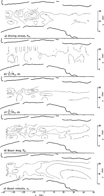
Fig. 10. Terms in the force budget in the y-direction and calculated τby, and basal velocity, uy. Like Figure 8 except that the more sophisticated calculation scheme is used.
The possibility of bottom crevasses is interesting. If there are bottom crevasses, there must be some other corresponding effect, such as increased stretching, ∂ux /∂ x , where the ice is thin, in order to satisfy slowly varying longitudinal force transmission. Longitudinal stretching ∂ux /∂ x , Fig. 2c) is, however, very small in this region and the expected stretching anomaly is within measurement precision. There should also be a surface hollow over the bottom crevasse, and indeed there does seem to be such a feature on Landsat imagery (called a “transverse ridge” in Reference Lucchitta, Bowell, Edwards, Eliason and FergusonLucchitta and others (1987, Fig. 10), but our interpretation of the shadow pattern indicates it to be a hollow).
Driving Stress
The driving stress

is calculated from data on thickness, H, and surface elevation, h. The ice density, p, is held constant at 0.91 Mg m−3, which allows for low-density firn or crevasse voids near the surface. Acceleration due to gravity, g, is 9.8 m s−2.
Surface slopes (Fig. 6b and c) are derived from the elevations, h (Fig. 6a) of Brecher’s first and better constrained photo survey. Generally the two elevation surveys agree to within 10–15 m and this is used to estimate the standard error in elevation. Taking the center of this range, each elevation survey is estimated to be precise to about 12m/(2)½. Consistent with this, the elevation grid is smoothed so that the standard deviation of its difference from Brecher’s elevations is 8.9 m.

Fig. 6. Gridded surface elevations and slopes. Contour interval for elevation is 25 m and for slope is 0.005.
The elevations in Reference MclntyreMcIntyre (1985) and Reference Dowdeswell and MclntyreDowdeswell and McIntyre (1987) are about 400 m higher than these and than elevations on earlier maps (USGS, 1966; Reference Drewry and DrewryDrewry, 1983). This we attribute to an error in Mclntyre’s and Dowdeswell and Mclntyre’s elevations. Their thicknesses, however, are taken as accurate.
The resulting two components of driving stress (Figs 7a and 8a) show small values where the glacier floats and are larger and variable where grounded. These variations are at a horizontal scale about three times the ice thickness, and are associated mainly with surface slope (Fig. 6b and c).

Fig. 7. Terms in force balance in the x-direction and calculated basal drag. τbx, using the simplification that strain-rates are constant with depth, cross-valley thickness is constant, and the stiffness parameter, B, is constant. Contour interval is 50 kPa.

Fig. 8. As Figure 7 but for terms in force balance in the y-direction.
This is because the surface slope undergoes more proportional variation than does thickness. Anticipated errors in the thicknesses are not expected to change the driving stress in an important way.
Force Balance for Isothermal Block Flow
The simplest calculations are for the case of strain-rates assumed constant with depth at the surface values, of thickness constant across the glacier, and constant stiffness parameter, B. Force balance is then written (part I):

in which surface values for Rxx , Ryy , and Rxy are used. The terms in this equation and the basal drags, τ bi , so calculated, are plotted in Figures 7 and 8.
The major features are near zero basal drag where the ice floats, as may be expected, and large and variable basal drag for the grounded part. Negative values for τ bx occur in very limited areas. These are difficult to accept and are associated with the restrictions of this simple block-flow model. Generally, the most important term on the right-hand side of the equation is the driving stress (Figs 7a and 8a). The gradient terms (Figs 7b and c and 8b and c) generally reduce the effect of fluctuations in driving stress, but there is a major exception near x = −27 km and −13 km, y = 12 km. This is associated with the “snaking” action noted above.
The block-flow calculations have the great merit of being simple to carry out. Although the limited regions of negative drag give cause for disquiet, there is qualitative similarity to the results presented next. The block-flow model is thus a viable first model, and leads to variations in basal drag that are substantially the same as those obtained below that allow for transverse thickness variations and depth-varying velocity.
Effect of Depth Variation in Velocity
Although the calculation for isothermal block flow is simple and instructive, velocities and strain-rates are usually expected to vary with depth. The force-budget calculation can be used to calculate velocities as a function of depth. The results of such a calculation following the methods in the second part of part I are shown in Figures 9 and 10. Bridging effects are small (part II) and are not included. To first order, the results for stresses are very similar to those for isothermal block flow.
For Byrd Glacier, the general effect of depth variation in velocity is to make the gradient terms in the force budget smaller. Horizontal velocities and strain-rates (![]() ,
, ![]() and
and ![]() ), on average, become more nearly zero with depth, and that makes the corresponding deviatoric stresses (σ′
xx
, σ′
yy
and σ′
xy
) more nearly zero. Shearing on horizontal planes (∂ux
/∂
z
and ∂uy
/∂
z
), however, becomes more important and that tends to raise the value of the effective strain-rate,
), on average, become more nearly zero with depth, and that makes the corresponding deviatoric stresses (σ′
xx
, σ′
yy
and σ′
xy
) more nearly zero. Shearing on horizontal planes (∂ux
/∂
z
and ∂uy
/∂
z
), however, becomes more important and that tends to raise the value of the effective strain-rate, ![]() (equation (1)). The net result is that the effective strain-rate approaches zero more slowly than the horizontal strain-rate components
(equation (1)). The net result is that the effective strain-rate approaches zero more slowly than the horizontal strain-rate components ![]() ,
, ![]() and
and ![]() , or may even increase with depth. Because the effective strain-rate is raised to a negative power in the flow law (equation (2)), its depth variation also contributes to making the deviatoric stresses σ′
xx
, σ′
yy
and σ′
xy
more nearly zero at depth. Thus, on average, the depth mean of these deviatoric stresses and the closely linked resistive stresses are nearer to zero than in the block-flow model.
, or may even increase with depth. Because the effective strain-rate is raised to a negative power in the flow law (equation (2)), its depth variation also contributes to making the deviatoric stresses σ′
xx
, σ′
yy
and σ′
xy
more nearly zero at depth. Thus, on average, the depth mean of these deviatoric stresses and the closely linked resistive stresses are nearer to zero than in the block-flow model.
Temperature at depth is also usually higher and that reduces the stiffness, B of the ice, further reducing the magnitude of horizontal stresses at depth. The stiffness parameter is taken to vary cubically with depth from a value of 630 kPa a1/3 at the upper surface to 180kPa a1/3 at the bed (which corresponds to values near the melting temperature) (Reference HookeHooke, 1981). This depth variation in stiffness parameter is probably too large. Scofield and others (paper in preparation) find that the temperature at the base for the grounded part must be less than the freezing point. So we may have over-corrected for the effect of temperature, exaggerating the difference from the isothermal block-flow model.
The effect of smaller resistive stresses at depth can be understood by studying the full equation for force balance (part I):

in which h and b represent surface and bed elevations, respectively. Because resistive stresses Rxi and Ryi usually are nearer to zero at depth than at the surface, the integrals and their gradients are also, on average, closer to zero than for the isothermal block-flow model. The basal drag is thus expected to be more nearly equal to the driving stress in this more accurate calculation. Comparison of Figures 9 and 10 with Figures 7 and 8 confirms this: horizontal stress gradients are less important in Figures 9 and 10 where the depth variation in stiffness parameter and velocity are taken into account.
Deep velocities are also a product of the calculation, and basal velocities are shown in the bottom panels of Figures 9 and 10. The x-component of velocity, as calculated, is not realistic. These basal velocities vary between 600 m a−1 and −150 m a−1 in the grounded part. Small regions of negative velocity are easily discounted as arising from the thickness used in the calculation being too large, and given the paucity of thickness data that is entirely possible. However, the large positive basal velocities lead to a problem in mass continuity.
The discharge, as calculated from these velocities, is about 50% larger in the upper part of the glacier than in the lower part. This 50% discrepancy cannot be accounted for by melting at the surface or bottom, and the elevation of the glacial surface is known not to be changing so dramatically (Reference BrecherBrecher, 1982). There is something in error with the calculated deep velocities.
This continuity problem would be resolved through the use of a larger rate factor (softer ice). Deep ice is then calculated to travel more slowly at the upper end of Byrd Glacier. However, in this case, and as found in part II, basal velocities for softer ice are calculated to be much more variable. This is because, for softer ice, the basal drag is more nearly equal to the driving stress and, as the driving stress is very variable in the grounded part, so too are calculated deep velocities. Deep velocities vary from values nearly equal to surface velocities to very small or even reversed. There is thus no value for the rate factor that leads to deep velocities that are reasonable along the entire flow band. A different form of the flow law is required in order to satisfy both slow and slowly varying deep velocity.
This improved flow law should be anisotropic. It should be stiffer to horizontal normal stresses than to shear stress on near-horizontal planes. By being stiff to horizontal stress, the role of the stress-gradient terms in the force budget is enhanced. Generally, this makes the calculated deep shear stresses vary less than the driving stress and so deep velocities would vary less. By being soft to shear or near-horizontal planes, deep velocities would be calculated to be smaller, as required to satisfy continuity. We recommend that flow laws of this type, as suggested by Reference Pimienta, Duval and LipenkovPimienta and others (1987), be used in future work.
Although the deep velocities calculated with the isotropic flow law are not realistic, the patterns in stress are meaningful. Use of a flow law that is stiffer to horizontal normal stresses would increase the amplitude of stress variations in panels b and c of Figures 9 and 10 but would have little qualitative effect on the results.
Stress Pattern
The x-component of basal drag varies between 0 and 300 kPa (Fig. 9d). It shows larger values up-glacier and near-zero values where the glacier floats. The scatter of values in the floating part is a measure of the level of imprecision in the data and technique and that is about 50 kPa.
The variations in basal drag are mainly associated with variations in driving stress (Fig. 9a), the only major exception being at x = −25 km, yu = 15 km. This conforms with results for inland ice (part II; Reference Whillans and JohnsenWhillans and Johnsen, 1983), where the basal drag correlates closely with the driving stress, but with reduced amplitude. On inland ice the difference is accommodated by differential longitudinal pushes and pulls ![]() and the reason for this has been addressed by Reference WhillansWhillans (1987). On Byrd Glacier, gradients in side drag
and the reason for this has been addressed by Reference WhillansWhillans (1987). On Byrd Glacier, gradients in side drag ![]() also contribute. The two force gradients work together in a complex way, but, in contrast with inland ice, neither correlates simply with the driving stress or basal drag. Gradients in side drag are important only near the center line in the grounded part (Fig. 9c). The reason for this is unclear. There may also be important side-drag gradients near the rock walls, but the data are inadequate to investigate that.
also contribute. The two force gradients work together in a complex way, but, in contrast with inland ice, neither correlates simply with the driving stress or basal drag. Gradients in side drag are important only near the center line in the grounded part (Fig. 9c). The reason for this is unclear. There may also be important side-drag gradients near the rock walls, but the data are inadequate to investigate that.
The y-component of basal drag, τby, is also somewhat similar in pattern to the corresponding driving stress, τdy. This again indicates mainly local, basal support of the glacier. Like the x-component of basal drag, τbx, it is of reduced amplitude compared to the driving stress. The reduction is mainly due to differential lateral tension (Fig. 10c or 4c) at x = −10 km. This may be associated with the tributary glacier which joins at x = −23 km, y = 3 km, or with the “snaking” flow discussed earlier.
This tributary, or some other effect, provides a compressive push of about −100 kPa (Fig. 4c) at x = −23 km and there is an opposing push of −150 kPa from the opposite side of the glacier at x = −13 km that returns the glacier to its nearly straight-line course. As noted earlier, this effect of the tributary is also evident in the flow-line turning, ∂u y /∂x (Fig. 3b). It also appears in deflections of ice-surface stream lines in Landsat images (Reference Lucchitta and FergusonLucchitta and Ferguson, 1986; Reference Lucchitta, Bowell, Edwards, Eliason and FergusonLucchitta and others, 1987). The agreement between the deflection of stream lines and the measured velocities indicates that the stream lines are flow lines and that the flow pattern has been stable for at least the approximately 25 years necessary to develop the pattern in the longitudinal stream lines.
The large cross-valley drag, τby, raises questions about glacial erosion. If erosion were related to basal drag and if the push at x = −23 km were a steady feature, then a deviation in channel shape at that site should have developed. That the valley is nearly straight indicates that there has been no important erosion or that the push at that site has not persisted for a long time. The former interpretation is supported by the reverse angle at which the small tributary joins near x = 18 km, y = 25 km. It too has not eroded a valley that favors its flow.
Discussion
An important result is the demonstrated inadequacy of the conventional isotropic flow law. Its use leads to unreasonable deep velocities and velocity variations. A different flow law is needed. An anisotropic flow law could account for an ice fabric in which vertically oriented c-axes are favored. It would be stiff to horizontal stress and soft to shear on near-horizontal planes. Such a flow law needs to be developed, perhaps along the lines of Reference Pimienta, Duval and LipenkovPimienta and others (1987). Other effects that could be included are strain history and variations in structure. We believe that data sets from places like Byrd Glacier are useful in testing the practical validity of proposed flow laws.
The problems with the flow law affect mainly deep velocities and the effects are so important that the calculated basal velocities lack physical significance.
The calculated stress pattern is, however, only weakly sensitive to uncertainties in the flow law. The effect is such that use of a rate factor corresponding to stiffer ice leads to larger horizontal stresses and generally more subdued variations in basal drag. However, the main patterns in stresses are not greatly affected by the flow law selected.
The maps of stress and force gradients make clear the relative importance of the various resistive forces. Tension from the ice shelf is about 100 kPa (Fig. 4a) and is relatively insignificant. The same map shows that tension from the inland ice is also unimportant. Reference HughesHughes (1986) argued for a large “pulling effect,” but the data do not extend up-glacier to the site of initiation of streaming flow where that effect is expected to be large. Side drag (Fig. 4b) is not very important. Rather, normal stresses dominate the horizontal stress regime and are locally very variable and of similar magnitude as the basal drag. The glacier is held mainly by basal drag, and that is concentrated at a very few sites separated by about 13 km.
The tension from the ice shelf may need explanation. The longitudinal strain-rate (Fig. 2c) is near zero and therefore so is the longitudinal deviatoric stress, σ′xx� Deviatoric stresses are, however, difficult to interpret in terms of force balance and that is especially true here. In this region there is lateral spreading (Fig. 2d) which, because ice is nearly incompressible, means that there is a tendency for longitudinal (and vertical) compression. There must be a tensile stress to counteract this tendency and the small extra tension, Rxx (Fig. 4c), as calculated here, is that tension. It arises from effects beyond the limits of the survey, and presumably helps balance the net driving force of the ice shelf.
The traditional view for ice shelves is to consider the stress in excess of that required for free spreading of the ice shelf. This excess stress is usually negative, or compressive, and is called the “back pressure” (Reference ThomasThomas, 1977). The lower end of Byrd Glacier does not spread in the x-direction so there must be a compressive back pressure in that direction. For the y-direction there is spreading and the back pressure in that direction is less compressive. There are, however, difficulties with the definition of back pressure and because of that Reference MacAyeal, Van der Veen and OerlemansMacAyeal (1987) defined a “dynamic” drag. MacAyeal’s dynamic drag is equivalent to the resistive stress used here, integrated through the thickness.
We remark here that there is no difficulty in the present scheme with coupling ice-shelf-style flow to grounded ice.
The sides of outlet glaciers and ice streams may be softened because of the development of a preferred crystal-orientation fabric or by the heat of dissipation. If either of these effects were included here, the value of side shear stress, Rxy , near the margins would be reduced. However, in this study side-shear stress and gradients in it are unimportant near the margins, even assuming that the ice is stiff (Figs 7c, 8b, 9c, and 10b). Allowing for these effects could reduce the value of Rxy calculated for the valley walls but not affect, in an important way, the calculations in the main part of the glacier.
The cause of fast, streaming flow such as for Byrd Glacier is not known. The stream lines observed on aerial photographs and Landsat images originate up-glacier of the part studied here. Reference Whillans, Bolzan and ShabtaieWhillans and others (1987) suggested that fast flow is enabled by large longitudinal and transverse normal stresses that make the ice soft to other stresses. This, however, is not a major feature of the studied section of Byrd Glacier. Rather, the effective strain-rate at the surface (Fig. 3d) is determined mainly by lateral shear, ∂ux /∂ y (Fig. 3a). The effect is the reverse of what Whillans and others proposed: on Byrd Glacier, lateral shear makes the ice soft to the normal stresses. The result is that horizontal normal stresses cannot be effectively transmitted through the margins and Byrd Glacier is largely decoupled from the valley walls.
There are very few thickness data, and they have been extended laterally in a very simple way. Because of this, certain results obtained must be viewed with caution. However, shortcomings in the thickness data are not as important a problem as the inadequacy of the isotropic flow law.
In terms of data, the major limitation lies with the velocity field. Reference BrecherBrecher (1986) obtained an approximately uniform density of velocites over the glacier, but a much higher density is needed near the lateral shear margins. Also, more careful work is needed on gridding the velocity data. The principal difficulty is that the longitudinal component of velocity, ux , has very strong across-valley gradients, ∂ux /∂ y and it proved difficult to find a gridding scheme that faithfully reproduces these gradients and yet smooths out local velocity variations consistent with known measurement uncertainties. In this regard, it should be noted that the major requirement in the study is not so much accurate velocities but accurate strain-rate gradients, that is, the second spatial derivative of velocity.
Other problems, such as developing a scheme to ensure that short-wavelength features do not arise in the calculation also need consideration. This is not a problem along the Byrd Station Strain Network (part II) and the reason for that is not clear. There the surface data are spaced by 3 km which is about the ice thickness. It may be that such a data spacing, in some way, inhibits the development of short-wavelength features in the calculation. In the present work, it proved necessary to smooth the velocities at each depth.
Acknowledgements
We thank H. Brecher for providing the data and for help in gridding them. This work was supported by an Ohio Board of Regents Research Challenge Award from The Ohio State University and the U.S. National Science Foundation (grant DPP-8517590). We thank K. Hutter and a referee for comments. Computer diagrams were improved by R. Tope. Typing is by C Gribbin. This is Byrd Polar Research Center contribution number 639.


