


Background
Ice discharge from tidewater glaciers is responsible for ~50% of the total mass loss from the Greenland ice sheet (GrIS) (Shepherd and others, Reference Shepherd2020), with this loss due to frontal ablation, comprising both iceberg calving and submarine melting (van der Veen, Reference van der Veen2002; Benn and others, Reference Benn, Warren and Mottram2007). Accurate prediction of total mass loss from the GrIS therefore requires detailed understanding of the principal controls on these processes. Iceberg calving is typically the dominant contribution to frontal ablation at tidewater glaciers in Greenland, with direct submarine melting a secondary effect (van der Veen, Reference van der Veen2002; Benn and others, Reference Benn, Warren and Mottram2007). However, recent modelling studies demonstrate that submarine melt-driven terminus undercutting and lateral heterogeneity in submarine melt rates across a glacier terminus can indirectly affect iceberg calving and thus overall ice loss (e.g. O'Leary and Christoffersen, Reference O'Leary and Christoffersen2013; Cowton and others, Reference Cowton, Todd and Benn2019).
The emergence of fresh subglacial runoff at glacier grounding lines generates buoyant turbulent plumes. These plumes enhance heat transfer across the ice–ocean boundary; as plumes rise, they entrain ambient fjord water which decreases the plume buoyancy and thus vertical velocity, but increases plume temperature (Jenkins, Reference Jenkins2011). A plume will continue to rise until it reaches neutral buoyancy with the ambient fjord water (Jenkins, Reference Jenkins2011; Kimura and others, Reference Kimura, Holland, Jenkins and Piggott2014), which may be at the fjord surface or at depth (Straneo and others, Reference Straneo2011; Slater and others, Reference Slater, Nienow, Cowton, Goldberg and Sole2015), with plumes generated by larger subglacial discharges typically rising higher in the water column (Carroll and others, Reference Carroll2015). Thus, meltwater plumes increase submarine melt rates for the portion of the glacier face in direct contact with the plume, relative to the melt rates for adjacent areas of the terminus (Kimura and others, Reference Kimura, Holland, Jenkins and Piggott2014; Slater and others, Reference Slater, Nienow, Cowton, Goldberg and Sole2015), which may still be affected but to a lesser extent (e.g. Slater and others, Reference Slater2018; Fried and others, Reference Fried2019; Jackson and others, Reference Jackson2020). Submarine melt rates across the calving margin (and the resultant terminus undercutting and enhanced iceberg calving) are therefore driven in part by spatial and temporal variations in the discharge of subglacial meltwater at glacier termini. This in turn is partly controlled by the routing of meltwater through the near-terminus subglacial hydrological system, the configuration of which may vary through a melt season (Slater and others, Reference Slater2017). We note here, that we refer to the configuration of near-terminus subglacial hydrology in relative terms (e.g. focused and distributed), in order to characterise any evolution in efficiency over the course of the melt season. We recognise that at times subglacial drainage may be in a relatively focused state, whereby meltwater is routed and consequently discharged through few, large portals. At other times the subglacial drainage may be in a comparatively distributed configuration, with subglacial runoff shared between multiple, smaller outlets at the grounding line (e.g. Slater and others, Reference Slater, Nienow, Cowton, Goldberg and Sole2015). This means that the delivery of an equivalent volume of subglacial meltwater to a glacier terminus, within different subglacial hydrological drainage configurations, may result in highly variable spatial patterns of discharge (and thus plume-driven terminus melting) across the grounding line.
For example, in a relatively focused subglacial drainage system, where water is discharged through few (1–2) portals at the grounding line, plume-enhanced submarine melting is localised, resulting in higher melt rates focused over a small portion of the glacier face (Fried and others, Reference Fried2015; Slater and others, Reference Slater2017). This spatially concentrated enhanced melting can drive morphometric change in the planform terminus shape (e.g. Chauché and others, Reference Chauché2014; Fried and others, Reference Fried2018; Jouvet and others, Reference Jouvet2018). Although studies have also indicated the potential for localised plumes to drive large-scale fjord circulation (and thus terminus-wide melting) (Slater and others, Reference Slater2018; Sutherland and others, Reference Sutherland2019), modelling suggests that spatially focused emergence of runoff results in lower rates of terminus-wide melting for an equivalent water discharge (Slater and others, Reference Slater, Nienow, Cowton, Goldberg and Sole2015), leading to reduced rates of iceberg calving and thus frontal ablation. In contrast, a more spatially distributed hydrological network with subglacial runoff dispersed between a greater number of smaller outlets at the grounding line (e.g. Slater and others, Reference Slater, Nienow, Cowton, Goldberg and Sole2015), results in reduced subglacial discharge through each portal. This subglacial hydrological configuration will generate lower velocity plumes reaching neutral buoyancy below the surface but with an increased proportion of the terminus experiencing plume-enhanced submarine melting and terminus undercutting (Slater and others, Reference Slater, Nienow, Cowton, Goldberg and Sole2015). Modelling studies suggest that this undercutting drives terminus instabilities, resulting in higher rates of iceberg calving and thus ice loss relative to a more focused subglacial hydrology (Benn and others, Reference Benn2017; Todd and others, Reference Todd2018).
Despite clear potential for the near-terminus subglacial drainage system to influence frontal ablation processes, how the spatial and temporal development of this system influences iceberg calving and thus ice loss remains poorly understood. There is a considerable lack of field-based observations to compare with model results and as such it has not been possible to constrain the influence of the near-terminus subglacial hydrology on overall frontal ablation. Recent studies utilising high spatial and/or temporal resolution data have revealed important insights into the mechanisms of iceberg calving at tidewater glaciers. For example, Medrzycka and others (Reference Medrzycka, Benn, Box, Copland and Balog2016), How and others (Reference How2019) and Vallot and others (Reference Vallot2019) used time-lapse imagery to show that different calving styles result from melt undercutting (e.g. leading to small waterline calving events, terminus instabilities and terminus-wide calving) and ice dynamics (e.g. enhanced crevasse propagation/hydrofracture).
Here, we aim to add to these high spatial and temporal resolution observational studies by analysing iceberg calving activity alongside proxies for controls on ice loss. We use high temporal resolution time-lapse observations (photos every 30 min) to detect iceberg calving events and the timing and location of visible meltwater plumes at Kangiata Nunaata Sermia (KNS), southwest Greenland, during June–October 2017. We analyse these observations alongside meteorological data, modelled estimates of meltwater runoff, satellite-derived ice velocities, terminus position and frontal ablation in order to investigate both short-term and seasonal controls on iceberg calving and ultimately, to improve understanding of the primary environmental drivers of calving processes over the course of the melt season.
Study area
KNS is the largest tidewater glacier in southwest Greenland, contributing 6.4 ± 1.9 Gt a−1 to the total ice discharge from the southwest portion of the ice sheet between 1978 and 2018 (Mouginot and others, Reference Mouginot2019) (Fig. 1). The ice front is ~5 km wide with a maximum grounding line depth of ~200 m below sea level (Morlighem and others, Reference Morlighem2017). KNS retreated ~25 km between its Little Ice Age maximum in 1761 and 2012 (Weidick and Citterio, Reference Weidick and Citterio2011; Lea and others, Reference Lea, Mair and Rea2014). Over the last ~20 years, KNS has experienced acceleration and thinning, but only minimal terminus position change on inter-annual timescales (~100 m a−1, Motyka and others, Reference Motyka2017).
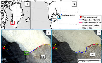
(a) Location of Godthåbsfjord (red square). (b) Location of KNS within Godthåbsfjord (blue square). (c, d) Time-lapse camera installation and terminus sub-sections (as described in the main text). The green squares highlight the approximate portion of the west section not visible by the time-lapse camera. These panels also indicate examples of the variable terminus geometries observed at KNS across the study period. These comprise a relatively ‘flat’ terminus (c) and a ‘crenellated’ terminus with a seasonal embayment (d). The base images are a Landsat 8 image from 22/07/17 (c) and a Sentinel-2 image from 05/09/17 (d).

Data and methods
Iceberg calving
We installed a time-lapse camera system in May 2017, on a bedrock ridge ~4 km west of the centre of the KNS calving front (64°17.964′ N, 49°42.481′ W). The camera was trained on the KNS terminus to capture calving and meltwater plume activity during the melt season (Fig. 1). The time-lapse system consisted of a Pentax K200D camera, a Pentax-DA 1:3.5–5.5, 18 mm zoom lens, and a Harbortronics Digisnap 2700 intervalometer, which was powered by a 12 V DC battery and a 10 W solar panel. The camera was programmed to take one photo every 30 min between 31 May and 31 October, resulting in 7392 images in total. Images were manually discounted when poor visibility obscured the calving margin and whole days were subsequently discounted and omitted from the analysis if more than 50% of the photos were obscured; this resulted in 13 d out of 151 (8%) being excluded from the analysis. Although the camera was installed in May, we were not able to record calving activity until 3 June due to a seasonally floating ice tongue (Moyer and others, Reference Moyer, Nienow, Gourmelen, Sole and Slater2017), which ensured it was not possible to determine the boundary between the glacier terminus and the ice tongue and mélange and also restricted iceberg calving.
To record and characterise spatial patterns in calving location, we divided the calving margin into three sections based on terminus behaviour and visibility: the west section (~1.9 km wide), where a seasonal embayment develops; the central section (~1.8 km wide), where a prominent prow develops during the melt season; and the east section (~1.3 km wide) (Fig. 1). To ensure that the delineation of the different terminus sections remained consistent across the time-lapse images, we used a cloud-free Sentinel-2 satellite image from 20 June (from the ESA Copernicus Open Access Data Hub, available at https://scihub.copernicus.eu), a time-lapse image from the same day and traceable features in both the satellite and time-lapse images (e.g. notches in the ice cliff, icebergs in the near-terminus fjord and prominent crevasse patterns), to ensure consistent pixel coordinate reference points between the sequential time-lapse images. We subsequently excluded the east section of the terminus from our analysis as it was partially obscured by the central section and was never fully visible in the time-lapse camera field of view. We also excluded the westernmost ~0.7 km of the terminus (green box in Fig. 1), as this section of the terminus retreated out of view during the time-lapse study period. In total we analysed ~3 km out of the 5 km width of the terminus (60%).
We classified iceberg calving events into three ordinal categorical magnitudes of ‘small’, ‘medium’ and ‘large’ using a reference grid overlaid on the subaerial ice cliff, to group calving event size relative to the height of the subaerial calving margin. The height of the subaerial calving margin at KNS is relatively consistent across the fjord (~50 m), as indicated by BedMachine (v3) (Morlighem and others, Reference Morlighem2017). We adopted this approach because we were unable to obtain the necessary ground control points to quantify the volume of individual calving events from our time-lapse imagery. We classified small calving events as those that spanned <25% of the subaerial ice cliff height (Table 1). These were primarily waterline or ice-fall calving events (Benn and others, Reference Benn, Warren and Mottram2007; How and others, Reference How2019). We classified medium calving events as those that spanned between 25 and 75% of the subaerial ice cliff height (Table 1). Medium calving events most frequently consisted of ice-fall events or isolated stack-collapses (Benn and others, Reference Benn, Warren and Mottram2007; How and others, Reference How2019). Large calving events were classified as events that spanned more than 75% of the ice cliff height and that may also have initiated multiple surrounding calving events (Table 1).
Classification of calving event magnitude (and example calving styles) relative to the height of the subaerial calving margin

Subglacial hydrology
To calculate daily runoff for KNS, we integrated modelled surface runoff from the 1 km resolution down-scaled version of the polar Regional Atmospheric Climate Model (RACMO v2.3) (Noël and others, Reference Noël2016), over a subglacial catchment derived from a hydropotential analysis (Shreve, Reference Shreve1972) constrained by BedMachine (v3) data (Morlighem and others, Reference Morlighem2017). Surface runoff was routed to the terminus assuming rapid transfer of meltwater to the bed and subsequent transport speeds commensurate with channelised drainage (1 m s−1) (Chandler and others, Reference Chandler2013; Cowton and others, Reference Cowton2013).
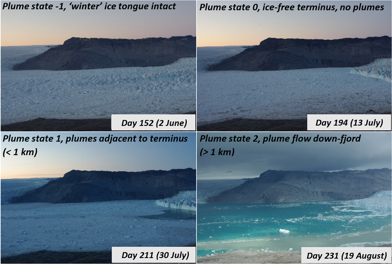
Using the time-lapse imagery, we recorded occurrences of plume expression at the fjord surface and classified each image into one of four states (following Slater and others, Reference Slater2017) (Fig. 2). Images showing the presence of the ‘winter’ ice tongue were assigned a value, −1. Images without the ice tongue but with no surface expression of a plume were assigned a value 0. Images showing the presence of a plume at the fjord surface were assigned a value of 1 or 2 respectively, depending on whether the surface expression of the plume was limited to within 1 km of the calving front (state 1) or whether the plume flowed down-fjord at the surface for over 1 km from the KNS calving margin (state 2).
Classification of plume visibility. Plume state = −1, seasonal ice tongue present; plume state = 0, no ice tongue and no surface plume presence; plume state = 1, plume presence within a kilometre of the terminus; plume state = 2, turbid plume present and flows down-fjord more than a kilometre from the terminus. Photographs are taken from the time-lapse camera (see Fig. 1).
In addition to estimated daily discharge, we use a postulated critical discharge threshold of 50 m3 s−1, as modelled by Slater and others (Reference Slater2017), to analyse the relation between subglacial runoff and the occurrence of visible meltwater plumes, in order to infer near-terminus subglacial hydrological characteristics. This threshold gives an approximate estimate of the minimum runoff that is required, for a single plume emerging at the glacier grounding line, to reach the fjord water surface in a modelled domain representative of the fjord's water properties immediately adjacent to KNS (Slater and others, Reference Slater2017). When subglacial runoff is greater than this threshold, the model predicts a plume would be visible at the fjord surface if runoff were emerging from a single outlet. Therefore, assuming that discharge emerges through point sources (indicative of a channelised drainage configuration) (e.g. Cenedese and Gatto, Reference Cenedese and Gatto2016; Slater and others, Reference Slater2017), the absence of any visible plumes indicates that no single channel can have a discharge greater than the critical threshold of 50 m3 s−1 (Slater and others, Reference Slater2017). We used this threshold to infer days on which plumes should theoretically be visible at the fjord surface. We combine this with the record of plume visibility from the time-lapse imagery as a proxy for the degree of spatial distribution of subglacial water emerging at the grounding line and use this to infer relative subglacial drainage system efficiency at daily resolution.
Although adopting a fixed estimate of the critical discharge, Slater and others (Reference Slater2017) tested how this threshold might have varied by considering substantial variations in fjord stratification, the presence of a freshwater surface layer and changes to sediment load and found that these sources of variation had limited impact on the estimated value of threshold discharge. Slater and others (Reference Slater2017) also investigated impacts on the estimated timing of the delivery of subglacial discharge to the grounding line, including variations in englacial storage times (McGrath and others, Reference McGrath, Colgan, Steffen, Lauffenburger and Balog2011) as this could potentially result in inaccurate inferences between modelled subglacial discharge and the visibility of plume surface expressions. This was accounted for by considering end-member transit velocities for both ‘rapid’ (1 m s−1) and ‘delayed’ (0.05 m s−1) runoff scenarios, intended to represent the upper and lower limits of potential seasonal variation in subglacial transit velocities over a melt season and also included ‘delayed’ scenarios to account for englacial storage. They found that selecting different transit velocities and storage ‘delay’ scenarios did not impact their inferences between subglacial discharge and plume visibility. We also emphasise that our current understanding of subglacial hydrology at tidewater glacier termini is limited. Previous studies have highlighted evidence for variability in the configuration of subglacial drainage systems at tidewater glaciers in Greenland and elsewhere, including for example observations of rapidly changing subglacial pathways (e.g. How and others, Reference How2017); subglacial discharge through outlets of varying dimensions (e.g. Fried and others, Reference Fried2015); and potential seasonal evolution of the near-terminus subglacial drainage configuration (e.g. Slater and others, Reference Slater2017). We therefore refer to near-terminus subglacial hydrology in relative terms; we infer that fewer, larger subglacial conduits would indicate a focused, more efficient subglacial hydrological system and a greater number of smaller conduits would represent a relatively more distributed and likely less hydraulically efficient subglacial drainage system. We use this terminology as a way of characterising any evidence for subglacial drainage evolution (with potential impacts on iceberg calving activity and ice loss) over the course of a melt season.
Terminus front position change
We acquired Sentinel-1A and -1B Interferometric Wide (IW) Swath Mode, Single Look Complex (SLC) Synthetic Aperture Radar (SAR) amplitude images (freely available from the ESA Copernicus Open Access Data Hub) (available at https://scihub.copernicus.eu). We use uncalibrated radar backscatter data, georeferenced and orthorectified based on the Greenland Ice Mapping Project (GIMP) Digital Elevation Model (DEM) (Howat and others, Reference Howat, Negrete and Smith2014, Reference Howat, Negrete and Smith2015) and posted at a spatial resolution of 20 m. Terminus retreat was calculated using the commonly adopted rectilinear box method, which accounts for asymmetric terminus migration (e.g. Moon and Joughin, Reference Moon and Joughin2008; Lea and others, Reference Lea, Mair and Rea2014). We quantified digitisation errors by repeatedly digitising a ~5 km section of rock coastline in five images. The resultant mean error was ±4.3 m, which is below the pixel size of our images.
Ice velocity
Ice velocity estimates were derived from feature and speckle tracking of Sentinel-1A and -1B IW Swath Mode SLC SAR amplitude images. Offsets between 6-d repeat image pairs at full resolution in radar coordinates were determined using normalised cross-correlation within PIVsuite in MATLAB (https://uk.mathworks.com/matlabcentral/fileexchange/45028-pivsuite) and subsequently projected to ground coordinates using the same method as the images used to determine terminus front position. We derived ice velocities for KNS between May and November 2017 with a median velocity error of 21.8 m a−1. The median error is based on a longer time series (2015–18) and was calculated by measuring the difference from zero of apparent velocities over bedrock. For full information on the methods used to derive ice velocities reported within this paper, refer to Tuckett and others (Reference Tuckett2019).
Frontal ablation flux
We calculated total width-averaged frontal ablation flux which represents ice loss from both calving and submarine melting. As we do not have direct estimates of submarine melting at KNS, we assumed that the ice cliff remained vertical over the course of the melt season (e.g. How and others, Reference How2019; Ma and Bassis, Reference Ma and Bassis2019) and that the position of the calving front is representative of total frontal ablation flux (i.e. that there is no significant ice toe). We first constructed a static flux gate, ~3.5 km upstream of the KNS terminus, to maximise data coverage (consistent with previous studies (e.g. Mankoff and others, Reference Mankoff2019)). To account for the impact of differential ice velocities across the glacier, we divided this flux gate into sections of equal width (1 km each). For each glacier section, we calculated width-averaged calving rates (c) (Eqn (1)) using the mean ice velocity (U) of the section and the width-averaged terminus length change (dL) over a given time period (dt) (usually 6 d):

We subsequently calculated the width-averaged frontal ablation flux (a) (Eqn (2)) for each section, by multiplying the width-averaged calving rate by the cross-sectional area of each section (A). We calculated the cross-sectional area, for the same 1 km sections used to derive the ice velocities, by deriving the mean bed depth across each section using BedMachine (v3) (Morlighem and others, Reference Morlighem2017):

We then summed the width-averaged frontal ablation fluxes for each section to derive total width-averaged frontal ablation flux for KNS over a given time period (usually 6 d).
Meteorological data
Daily mean air temperatures were acquired from the nearby Geological Survey of Denmark and Greenland (GEUS) PROMICE meteorological station (NUK_L, 550 m a.s.l., 64°28.921′ N, 49°31.848′ W) (Ahlstrøm and others, Reference Ahlstrøm2008), ~21 km from KNS (see Fig. 1), using a lapse rate of 0.5°C per 100 m (Slater and others, Reference Slater2017) to adjust the air temperatures to sea level.
Results
Results from the time-lapse analysis of iceberg calving activity and meltwater plume visibility are shown in Figure 3. For the purposes of our analysis, the results are broken down into four phases. These phases were determined based on the differential characteristics of iceberg calving activity and plume presence during the observation period, as discussed in the results below. Our analyses use the mean number of calving events per day during each phase, alongside daily calving frequency, in order to allow for valid comparisons between phases despite their variable lengths.
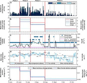
Results from the analysis of time-lapse images, meteorological and remote-sensing data. In all panels, dotted lines refer to mean values of the data for each phase within the study period. Phases are identified by solid, red vertical lines and labelled above panel (a). (a) Daily record of calving events from 3 June to 31 October 2017. Each bar represents 1 d of iceberg calving and the stacked bars represent the number of different magnitude events for that day. Grey hatched areas are from days when cloud obscured the terminus. (b) Daily mean calving frequency (defined as number of events per day), as in panel (a) for each phase. Note the different left and right axes. (c) Left axis. Daily record of plume visibility from time-lapse images. See Figure 2 for explanation of plume state classifications. Right axis. Modelled mean daily catchment runoff (black solid line), mean runoff during each phase (dotted blue line) and the postulated critical threshold for visible plumes (50 m3 s−1) (purple solid line). (d) Left axis. Mean daily air temperature from the NUK_L PROMICE meteorological station. Right axis. Width-averaged 6-daily ice velocity derived from Sentinel-1 SAR images. (e) Left axis. Mean daily terminus position change for each phase (dotted light blue line). Note the reverse direction of the y-axis to allow for ease of comparison with mean daily frontal ablation flux (right axis). Right axis. Mean daily frontal ablation flux (dotted dark blue line) for each phase (see Eqns (1–2)).

Phase 1 (3–24 June)
Phase 1 started following the disintegration of the seasonally floating ice tongue on 3 June. Before this date, the ‘winter’ ice tongue obscured the summer calving margin (Fig. 2), thereby preventing reliable observations of calving activity. Our time-lapse images showed that after the ice tongue disintegrated, the resulting brash ice from the tongue disintegration was flushed down-fjord and away from the terminus within several hours; a process and rate of evacuation that has been observed in other melt seasons (e.g. Slater and others, Reference Slater2017). Phase 1 was characterised by consistent but low frequency calving (Fig. 3a), with 155 calving events in total (seven events per day, SD 3.1 events per day) including 24 large calving events (0.95 events per day). There was no spatial pattern to the calving events across the terminus. Despite a low calving frequency, both mean daily front position change (−16.1 m d−1) and mean frontal ablation flux (0.014 km3 d−1) were the highest of the study period. However, mean ice velocity during phase 1 was the second lowest during the study period (8.6 m d−1) (Fig. 3d) and no meltwater plumes were visible, despite a mean discharge of 145 m3 s−1 (~3 times the critical threshold of 50 m3 s−1) and a peak discharge of 375 m3 s−1 (Fig. 3c).
Phase 2 (25 June–18 July)
Phase 2 was characterised by a step change in the frequency of iceberg calving events which occurred prior to the onset of visible meltwater plumes (Fig. 3a–c). Although the mean number of large calving events during phase 2 (1.2 events per day) was slightly greater than phase 1 (0.95 events per day), overall calving frequency (425 calving events, mean 19.8 events per day, SD 10.5 events per day) increased by a factor of ~3, due to an increase in the number of small- and medium-sized calving events. As in phase 1, calving events occurred across the entire observed calving front. The high frequency and magnitude of the calving events is reflected both in the mean daily front position change (−11.1 m d−1) and mean frontal ablation flux (0.012 km3 d−1) (Fig. 3e), which both represent the second highest values for these observations during the study period. Mean air temperature (0.83°C) and runoff (236 m3 s−1, and a peak discharge of ~675 m3 s−1) were higher than during phase 1 (0.44°C and 145 m3 s−1) (Fig. 3c). Mean ice velocity (8.8 m d−1), was only slightly greater than during phase 1 (8.6 m d−1) and was the highest recorded ice velocity of the study period.
Phase 3 (19 July–20 August)
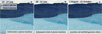
The onset of Phase 3 was delineated by the first visible plume on 19 July and covers the period of the melt-season characterised by the highest sustained runoff (mean discharge 359 m3 s−1). Calving frequency decreased (426 calving events in total, mean 13.3 events per day, SD 7.1 events per day) (Fig. 3a) with a substantial decline in both large- (0.4 events per day during phase 3 vs 1.2 events per day during phase 2) and medium-sized (2.6 events per day during phase 3 vs 4.3 events per day during phase 2) calving events relative to phase 2. Mean daily front position change (−2.2 m d−1) and mean frontal ablation flux (0.007 km3 d−1) also decreased by 80 and 42% respectively in comparison with phase 2 (Fig. 3e). Mean air temperature was at a seasonal high during phase 3 (Fig. 3d) with a 2°C increase (to 2.85°C) compared to phase 2 (0.83°C) whereas mean ice velocities decreased slightly between phases 2 (8.8 m d−1) and 3 (8.7 m d−1) (Fig. 3d). The onset of the first visible plume during the melt-season coincided with a rapid increase in runoff to 679 m3 s−1 (~3 times greater than mean runoff during phase 2) (Fig. 3c). At the start of phase 3 (19–27 July), multiple plumes in state 1 were observed across the entire terminus (Fig. 4a). Once the plumes developed to state 2 on 28 July, the number of plumes visible at the surface decreased, with plumes only visible subsequently in two locations: in a seasonal embayment and in the vicinity of a prow that both form during phase 3 (Figs 1 and 4b–c). Throughout the remainder of the melt season, when plumes oscillated between states 1 and 2, they remained located in these same two locations (Fig. 4b and c).
Time-lapse image with example plume locations for each period of differential plume activity during phase 3. (a) During 19–27 July we observed plumes well distributed across the terminus. (b) During 28–31 July we observed a concentration of plumes in proximity to the prow and seasonal embayment. (c) Towards the end of phase 3 and in phase 4 we observed oscillating plume states, but locations remained at the prow and seasonal embayment. For comparative purposes, due to the changes in the calving front position and shape (see Fig. 1) over the melt season and to understand plume locations relative to the previous phase, we use a base image from 19 July, the first day that plumes were visible during the melt season.

Phase 4 (21 August–31 October)
The onset of Phase 4 was defined by a considerable decrease in runoff (relative to all previous phases) and infrequent plume surfacing (Fig. 3c). During phase 4, mean air temperature (−2.43°C) and ice velocity (8.5 m d−1) both decreased to their minimum during the study period (Fig. 3d). Phase 4 was characterised by a considerable decrease in the frequency of iceberg calving events of all magnitudes and this calving activity primarily remained restricted to the embayment and prow (326 calving events in total, 4.5 events per day, SD 4.4 events per day). This reduction in activity was reflected in mean frontal ablation flux that was the lowest during the study period (0.005 km3 d−1), with a 61% decrease from phase 2. The KNS margin also experienced an overall advance (1.5 m d−1) (Fig. 3e). Mean discharge during phase 4 was substantially lower than for any other phase (62 m3 s−1), with runoff negligible (<20 m3 s−1) for ~70% of the time with just three brief periods of high runoff driven by transient spikes in atmospheric temperatures (Fig. 3c–d). Plumes were visible on just 4 d, principally corresponding with the first and largest high runoff event and their emergence was solely focused within the seasonal embayment and in the vicinity of the prow (Figs 1 and 4).
Discussion
In this section, we synthesise the observed seasonal evolution of iceberg calving and subglacial hydrology at KNS and discuss the implications for ice loss and dynamics at both KNS and tidewater glaciers around Greenland.
Early-melt season (phases 1 and 2)
The onset of visible calving is coincident with the rapid disintegration of the seasonal floating ice tongue at KNS on 3 June at the start of phase 1. We argue, as observed elsewhere, that the reduction in buttressing, resulting from the loss of the ice-tongue here (similar to ice mélange disintegration seen elsewhere), is a key control on the onset of seasonal calving and of subsequent terminus retreat (e.g. Amundson and others, Reference Amundson2010; Walter and others, Reference Walter2012; Moon and others, Reference Moon, Joughin and Smith2015). Based on evidence from observational and modelling studies, we suggest that the removal of the ice-tongue likely drives a near-instantaneous response of the glacier, initiating rapid iceberg calving and thus substantial ice loss at the onset of phase 1 (Walter and others, Reference Walter2012; Robel, Reference Robel2017; Todd and others, Reference Todd2018; Xie and others, Reference Xie, Dixon, Holland, Voytenko and Vaňková2019). This response is reflected in a seasonal high in both mean daily retreat and mean frontal ablation flux during phase 1 (Fig. 3e) promoted by particularly large calving events (Fig. 3a) (although the frequency of ‘large’ calving events was slightly lower in phase 1 compared to phase 2) (0.95 compared to 1.2 events per day respectively).
During both phases 1 and 2, modelled subglacial runoff was, at times, over seven times greater than the critical threshold (50 m3 s−1) postulated by Slater and others (Reference Slater2017) required for plumes to reach the surface of the KNS fjord. Despite this, no meltwater plumes were visible during either phase. We infer that the lack of plume surfacing suggests that subglacial runoff was spatially distributed across the grounding line such that the runoff from any individual outlet was less than the critical discharge. Although the critical runoff required to induce plume surfacing will likely vary throughout a melt season, principally due to changes in the density profile of ambient water, sensitivity studies (e.g. Slater and others, Reference Slater2017) demonstrate that this variability cannot explain the lack of plume surfacing during the early part of the melt season (since the critical threshold was always far less than the modelled runoff values). From these observations, we therefore infer that in the early melt season, water was emerging in a more spatially distributed manner across the grounding line at the terminus of KNS; we are however unable to determine the hydraulic characteristics of this spatially distributed configuration.
Several studies have shown that where meltwater emerges in a distributed configuration (as we infer during phases 1 and 2 at KNS), rather than a focused configuration, a greater proportion of the calving front is exposed to plume-induced submarine melting, theoretically leading to a factor 4–7 increase in submarine melt rates averaged over the calving front (Fried and others, Reference Fried2015; Slater and others, Reference Slater, Nienow, Cowton, Goldberg and Sole2015). Furthermore, spatially-distributed plume-driven submarine melting has been associated with undercutting of glacier termini elsewhere in Greenland (e.g. Fried and others, Reference Fried2015; Rignot and others, Reference Rignot, Fenty, Xu, Cai and Kemp2015; Carroll and others, Reference Carroll2016), which in turn may lead to increased calving rates (e.g. O'Leary and Christoffersen, Reference O'Leary and Christoffersen2013; Schild and others, Reference Schild2018; Todd and others, Reference Todd2018). Although we do not have submarine melt rate estimates for KNS, our inferences are in line with the findings of these studies: we observed the highest calving frequencies and highest rates of frontal ablation flux during the early melt season at a time when calving events were also distributed across the entire width of the visible terminus. We suggest that after the initial increase in iceberg calving at KNS in response to the disintegration of the ice-tongue in phase 1, the enhanced calving activity and sustained high frontal ablation flux observed in phase 2 reflect submarine-melt driven undercutting of large portions of the glacier terminus and we infer that this in turn is likely promoted by a distributed emergence of subglacial runoff. In addition to these observations, we observed a step-change in calving frequencies between phase 1 and 2, when modelled runoff increased. This increase in runoff without a concurrent increase in plume surfacing suggests further distribution of subglacial meltwater through multiple, distributed runoff outlets, thus exposing a greater portion of the terminus to runoff-enhanced submarine melting, and/or greater melt rates at existing outlets, thereby increasing terminus undercutting in those locations. Our observations suggest that this in turn promoted a much higher frequency of both ‘medium’ and ‘small’ calving events in phase 2, with the overall effect of sustaining the high frontal ablation flux originally initiated by the disintegration of the ice-tongue at the beginning of phase 1 (Fig. 3e); behaviour consistent with modelling studies (e.g. O'Leary and Christoffersen, Reference O'Leary and Christoffersen2013; Schild and others, Reference Schild2018; Todd and others, Reference Todd2018, Reference Todd, Christoffersen, Zwinger, Råback and Benn2019).
Melt season peak (phase 3)
The initial distribution of multiple state 1 plumes along the width of the glacier front from 19 to 27 July (Fig. 4a) demonstrates that although subglacial discharge was still distributed between multiple outlets, the runoff volume at numerous subglacial outlets was now sufficient to generate plumes capable of reaching the fjord surface (but not large enough to remain at the surface as in plume state 2). Once the plumes developed to state 2 on 28 July, their presence became laterally restricted to only the seasonal embayment and the prow (Fig. 4b). We suggest that this focusing of plume emergence results from the evolution of the subglacial hydrological system whereby meltwater is routed into fewer more hydraulically efficient subglacial channels (e.g. Sole and others, Reference Sole2011; Slater and others, Reference Slater2017). Without such an evolution, we would expect (based on the high modelled runoff volumes relative to the critical runoff threshold) the ongoing visibility of plumes at multiple, distributed sites across the terminus. This focusing of the subglacial drainage system is further supported by the fact that for the remainder of the melt-season, when plumes oscillated between states 1 and 2 (Fig. 3c), they remained visible only within the embayment and at the prow (Fig. 4c). This suggests the persistence of relatively efficient (in comparison with phases 1 and 2), focused subglacial drainage during phase 3 and into phase 4 even during times when runoff was significantly reduced.
Following the development of the first state 2 plume on 28 July, we observed a reduction and focusing of calving activity and a decline in mean frontal ablation flux rates in comparison to the early-melt season (Fig. 3e). State 2 plume locations were spatially and temporally coincident with changes to the KNS terminus planform geometry with the development of an embayment and prow (Fig. 1). The reduction in calving was temporally coincident with the first state 2 plume (Fig. 3c) and calving activity that did occur was primarily restricted to the embayment. Despite the presence of state 2 plumes, plume surface-expression was narrow (<800 m) relative to the width of the terminus (~5 km). Given that buoyant plumes expand in radius, entraining ambient water as they rise through the water column (Jenkins, Reference Jenkins2011), plume surface expression represents the maximum width of a plume. Our observations of a narrow surface expression (<800 m) therefore indicate that the fraction of the calving front directly affected by plume-driven submarine melting was small. Elsewhere across the terminus (i.e. outside the plumes), submarine melt rates are theoretically an order of magnitude lower (Fried and others, Reference Fried2015; Slater and others, Reference Slater2017) and a pronounced lateral heterogeneity in submarine melt rates (due to a focusing of emergent runoff) is therefore expected during this time, leading to the development of notches or crenellated terminus geometries as observed at other glaciers (e.g. Chauché and others, Reference Chauché2014; Fried and others, Reference Fried2018; Jouvet and others, Reference Jouvet2018) and here at KNS (Fig. 1). Our results therefore suggest that focused subglacial runoff has less impact on calving (and thus frontal ablation) than when runoff emerges in a spatially distributed manner at the grounding line. Whether this difference in calving response is due to the spatial pattern of melting, the absolute magnitude of melt rates, or some combination of both remains unclear. We also stress that we treat this inference with caution because we do not have submarine melt rate estimates at KNS and the links between undercutting and calving remain unclear (Benn and Åström, Reference Benn and Åström2018).
Late-melt season (phase 4)
At both the onset of and during phase 4, there was a pronounced drop in air temperature and thus runoff (~6 times decrease in mean runoff) relative to phase 3, with only occasional plume visibility. During these plume-surfacing events, plumes continued to emerge at just the two discrete sites (Fig. 4c) suggesting that the near-terminus subglacial drainage system remained in a focused configuration until at least 10 September. The considerable decrease in runoff coincided with a decrease in the frequency of calving events of all magnitudes (with a decrease in mean frontal ablation flux from 0.007 km3 d−1 during phase 3 to 0.005 km3 d−1 in phase 4 (Fig. 3d)) resulting in KNS undergoing terminus advance during this phase (1.5 m d−1 (Fig. 3d)). Despite a slight deceleration relative to phase 3 and a steady deceleration throughout phase 4 (Fig. 3c), mean ice velocity during this phase remained high (8.5 m d−1), implying a potentially high-pressure subglacial system irrespective of drainage configuration, likely due to the pressure exerted by the adjacent ~200 m fjord water column. No plumes were visible after 11 September, likely due primarily to negligible melt and runoff (Fig. 3c) but also possibly due to the gradual closure of subglacial channels and re-establishment of a more distributed subglacial drainage system preventing plumes being visible on the rare occasions (e.g. 20 September) when runoff was high (~500 m3 s−1).
Implications of near-terminus hydrology for ice loss
We suggest that during the 2017 melt season at KNS, evolution of the subglacial drainage system during the latter half of the melt season resulted in a pronounced reduction in calving magnitude and frequency (and therefore frontal ablation) (Fig. 3e). Our observations show that in the early part of the melt season, when we infer subglacial discharge to have been more spatially distributed, mean glacier-wide frontal ablation flux was considerably higher than latter in the melt season, when we infer (from plume surfacing) an evolution of the subglacial drainage system towards a more channelised state. We infer that this decrease in mean glacier-wide frontal ablation flux later in the melt season is due to a focusing of emergent subglacial runoff. This leads to reduced terminus-wide submarine melt rates and thus reduced iceberg calving in areas of the calving front distal to meltwater-driven plumes (Fig. 4b and c), despite presumably higher localised melt rates and recession, as we infer and observe respectively, in the vicinity of the observed surfacing plumes (Fig. 1) (e.g. Chauché and others, Reference Chauché2014; Kimura and others, Reference Kimura, Holland, Jenkins and Piggott2014; Schild and others, Reference Schild2018; Todd and others, Reference Todd2018). Our observations suggest that despite considerable morphometric terminus change (Fig. 1), the overall impact of a more channelised subglacial discharge (and thus more focused submarine melt) is to reduce calving rates and overall frontal ablation flux at KNS (phase 3 vs phases 1 and 2). We propose that these same processes potentially impact ice loss at a range of tidewater glaciers across Greenland and other glaciated regions.
Our results support studies that highlight the importance of submarine melting on iceberg calving and thus overall frontal ablation (e.g. Truffer and Motyka, Reference Truffer and Motyka2016; Benn and others, Reference Benn2017; Todd and others, Reference Todd2018; Ma and Bassis, Reference Ma and Bassis2019; Wagner and others, Reference Wagner2019). We argue that it is the spatial distribution of meltwater emergence that has a critical impact upon calving activity and frontal ablation. Specifically, the highest frontal ablation flux rates occurred at times when we infer meltwater emergence across a large proportion of the grounding line, and frontal ablation flux rates decreased once runoff became limited to just a few outlets. However, although we infer this link between frontal ablation and subglacial hydrology at KNS, it may not hold true (or indeed, the relation may be different) for all tidewater glaciers; there are a variety of characteristics intrinsic to individual tidewater glaciers that may influence the relation between submarine melting and iceberg calving and thus overall frontal ablation. For example, the impact of basal topography on both the routing of subglacial meltwater, which influences the spatial emergence of plumes and the terminus grounding line depth, which contributes to the height of plume neutral buoyancy (i.e. regardless of velocity or buoyancy, plumes emerging at a deeper grounding line may reach neutral buoyancy lower in the water column, compared to plumes emerging at a shallower grounding line (e.g. Carroll and others, Reference Carroll2016; Rignot and others, Reference Rignot2016; Todd and others, Reference Todd, Christoffersen, Zwinger, Råback and Benn2019)). Furthermore, there may be additional complex ice–ocean interactions, as suggested by recent studies that have revealed the role of plume-driven fjord-scale circulation in enhancing terminus-wide melting (e.g. Slater and others, Reference Slater2018; Sutherland and others, Reference Sutherland2019). These additional processes are also likely to vary in response to glacier and fjord-specific characteristics including complexities in fjord water stratigraphy and temperature (e.g. Mortensen and others, Reference Mortensen2020) which may be driven both by local and ocean and atmospheric forcing (e.g. Meire and others, Reference Meire2016), as well as by variations in glacial runoff and the subglacial drainage structure. Additional study is therefore required, necessitating both improved observations and modelling (e.g. Catania and others, Reference Catania, Stearns, Moon, Enderlin and Jackson2020), to understand the relation between near-terminus hydrology and iceberg calving for tidewater glaciers at an ice-sheet wide scale.
Conclusions
Our detailed observations of terminus calving, frontal ablation, plume activity, ice velocity and modelled runoff reveal that the spatial distribution of subglacial runoff at the grounding line of a large tidewater glacier in Greenland exerts a strong control on calving frequency and frontal ablation during the melt season. At the start of the melt season, we infer a distributed and inefficient near-terminus subglacial drainage system, which theoretically exposes a large proportion of the terminus to plume-enhanced submarine melting, promoting widespread terminus undercutting and rapid frontal ablation. The formation of hydraulically efficient channels during the melt season increasingly localises plume-driven melt to a decreasing number of locations across the calving front. Although iceberg calving rate remains high in these locations, it decreases elsewhere, leading to an overall reduction in mean frontal ablation flux. These results demonstrate how changes in subglacial drainage configuration can drive both spatial and temporal variations in submarine melt and associated calving processes and terminus dynamics. Our observations also highlight the difficulties associated with deducing simple scalings between glacier runoff and submarine melting (or frontal ablation), which would be desirable to support ice flow models linking ice-sheet surface melt to tidewater glacier terminus dynamics. Finally, given the expected increases in meltwater runoff in a warming climate, further changes in near-terminus subglacial hydrological characteristics should be anticipated, with associated implications for frontal ablation. However, the broader influence of these changes on frontal ablation, glacier dynamics and overall ice mass loss is yet unknown and may vary between glacier systems. It is therefore essential that the potential significance of terminus hydrology on calving processes is investigated further, in order to better incorporate these processes in modelling efforts attempting to constrain the future dynamics of tidewater glacier termini.
Acknowledgements
Charlie Bunce is supported by a NERC DTP studentship (NE/L002558/1). Ben Davison is funded by the Scottish Alliance for Geoscience, Environment and Society (SAGES) and University of St. Andrews. We acknowledge field and research grants from the RGS-IBG postgraduate research fund and Mackay/Weir Greenland Fund (University of Edinburgh) awarded to Charlie Bunce and RGS-IBG postgraduate research fund, Mackay/Weir Greenland Fund (University of Edinburgh) and Centenary Funding (University of Edinburgh) awarded to Alexis Moyer (University of Edinburgh). Sentinel-1 and Sentinel-2 images were acquired from ESA Copernicus Data Hub (scihub.copernicus.eu). We thank Brice Noël for supplying RACMO v2.3 data. We thank Alexis Moyer, Dominik Fahrner and Jakob Abermann for support in the field. We also thank the Scientific Editor William Colgan, Jason Amundson and two anonymous reviewers for their constructive comments that helped to improve the manuscript.
Author contributions
CB designed research with PN. CB performed all of the analysis and led the writing of the manuscript. AS and BD processed the Sentinel-1 images and ice velocities. BD produced the runoff estimates. All authors provided comments on the manuscript.


 Open access