


1. Introduction
All biological production processes are exposed to biological shocks such as disease and adverse weather conditions. In general, these exogenous shocks will have a limited market impact, as shocks that do not influence a large share of the production will readily be adjusted by market arbitrage (Stigler, Reference Stigler1969). However, in cases where a shock affects a sufficiently large part of production, the market impact of that shock can be substantial. Seafood-related examples are El Niños (Asche, Oglend, and Tveteras, Reference Asche, Oglend and Tveteras2013; Ubilava, Reference Ubilava2014), the hypoxia dead zones in the Gulf of Mexico (Smith et al., Reference Smith, Oglend, Kirkpatrick, Asche, Bennear, Craig and Nance2017), and environmental shocks in Norwegian salmon production (Asche, Oglend, and Kleppe, Reference Asche, Oglend and Kleppe2017), and mad cow disease is the most well-known example in food production in general.Footnote 1 Although there is a literature investigating the impact of such shocks on demand, there has been less focus on price determination and trade flows. In this article, a number of hypotheses with respect to market integration for salmon from Chile are tested, where production was reduced to a third because of a significant disease outbreak in 2010 (Fischer, Guttormsen, and Smith, Reference Fischer, Guttormsen and Smith2017).
Chile is the second-largest producing country of farmed Atlantic salmon (hereafter salmon), the most important species on the salmon market (Asche, Reference Asche2008).Footnote 2 Chile's output reached 403,000 metric tons (mt) in 2008, before it was more than halved in 2009, and plunged to 130,000 mt in 2010. Production rebounded rapidly after 2010, reaching 460,000 mt in 2013 when Chile had largely recovered its production share and has continued to increase since (Food and Agriculture Organization of the United Nations [FAO], 2017). The main reason for this dip in production was an outbreak of infectious salmon anemia (ISA), a viral disease with mortality rates of up to 100% in the worst cases (Asche et al., Reference Asche, Hansen, Tveteras and Tveterås2009; Fischer, Guttormsen, and Smith, Reference Fischer, Guttormsen and Smith2017; Quezada and Dresdner, Reference Quezada and Dresdner2017). Because of the disease outbreak, in Chile, fish were harvested earlier and therefore at smaller sizes (Asche et al, Reference Asche, Hansen, Tveteras and Tveterås2009). As different markets have varying preferences with respect to size (Asche, Reference Asche2001; Asche and Sebulonsen, Reference Asche and Sebulonsen1998), the change in the physical size of the harvested Chilean salmon precipitated a substantial shift in the markets being served as well as in the exported product forms.Footnote 3 Of particular interest in this case is the development of Brazil as a market for whole fresh Chilean salmon of moderate size, as exports to Brazil increased strongly during the crisis despite the reduction in total production. At the same time, there was a strong decline in exports of fresh fillets to the United States, a premium product form that requires larger fish for its production.
Disease and other contamination incidents potentially leading to unsafe food products can cause a significant decline in consumer demand and substantial losses in sales, both for the contaminated product and for the uncontaminated products that are close substitutes. This has been documented in a number of studies for various foods (Bakhtavoryan, Capps, and Salin, Reference Bakhtavoryan, Capps and Salin2012; Burton and Young, Reference Burton and Young1996; Fousekis and Revell, Reference Fousekis and Revell2004; Piggott and Marsh, Reference Piggott and Marsh2004; Pritchett et al., Reference Pritchett, Johnson, Thilmany and Hahn2007; Uchida, Roheim, and Johnston, Reference Uchida, Roheim and Johnston2017; Verbeke and Ward, Reference Verbeke and Ward2001), as well as specifically for salmon (Liu, Lien, and Asche, Reference Liu, Lien and Asche2016; Sha et al., Reference Sha, Insagnaris, Roheim and Asche2015). Several studies have also demonstrated a country-of-origin effect for salmon (Asche and Sebulonsen, Reference Asche and Sebulonsen1998; Asche et al., Reference Asche, Larsen, Smith, Sogn-Grundvåg and Young2015; Bronnmann and Asche, Reference Bronnmann and Asche2017; Uchida et al., Reference Uchida, Onozaka, Morita and Managi2014) and source-differentiated demand (Dey et al., Reference Dey, Rabbani, Singh and Engle2014; Muhammad and Jones, Reference Muhammad and Jones2011; Zhang, Tveteras, and Lien, Reference Zhang, Tveteras and Lien2014), indicating that a disease shock has the potential to segment the market. Moreover, the decrease in demand because of a disease outbreak can result in a substantial lowering of the price. A disease shock will also reduce the quantity available, as there would be a decrease in supply.Footnote 4 This can in turn lead to increased prices. Asche and Sikveland (Reference Asche and Sikveland2015) observe that prices and profits for Norwegian producers increased in response to the reduction in supply that resulted from the Chilean disease challenges, hence suggesting that the supply effect was dominant.
Whether and how the various producers benefit from increasing prices depends on the degree of substitutability between the products from the disease-exposed country and the products from other producers. If Chilean salmon is not differentiated from other producers’ salmon, the latter stands to face the same challenges because of a potential reduction in demand but will also receive the price benefits because of the limitation in supply. If the salmon market is segmented, limiting substitution between Chilean salmon and other salmon, then non-Chilean producers will have a lower risk of incurring losses, but also a lower potential for gains. Asche, Bremnes, and Wessells (Reference Asche, Bremnes and Wessells1999) indicated that there is a global market for salmon, comprising all salmon species. However, the link between the American market and the rest of the word is weaker than between the European and the Asian markets (Asche, Reference Asche2001), and Landazuri-Tveteras et al. (Reference Landazuri-Tveteras, Asche, Gordon and Tveteras2017) indicate that substitution is weaker between different product forms. This is important because Chile is typically the main supplier to the American market (with Canada as the second-largest supplier), whereas the other main producers, Norway and Scotland, primarily supply Europe and Asia. Moreover, fillets are the most important product form from Chile, whereas most other exporters have whole fresh salmon as the clearly most important product form.
Despite Chile being the second-largest producer, the degree of market integration for Chilean salmon relative to the global market has not been investigated in the literature. As Chile is the main supplier to the American market, the results of Asche (Reference Asche2001), supported by Xie and Zhang (Reference Xie and Zhang2014), indicate that there is some potential for segmentation. Hence, the shock caused by the disease outbreak in Chile can provide additional insights into the strength of market integration for salmon. In particular, it can indicate if the market integration becomes so weak that there is no longer a global market, or if other producers are able to adjust the trade patterns enough to maintain a global market.Footnote 5 In this article, the degree of market integration is investigated between four product forms of Chilean salmon—fresh and frozen whole and fresh and frozen fillets—and for the fresh product forms, the largest markets, Brazil and the United States, are also considered. Additionally, with Norway being the largest producer, the link to the Norwegian salmon price is investigated. Because all prices are nonstationary, the market integration analysis is conducted using the Johansen cointegration test.
The article is organized as follows: A description of the Chilean salmon industry and a description of the available data are first provided. A section is dedicated to methods, with the empirical results reported thereafter. Finally, some concluding remarks are offered.
2. Background and Data
The Chilean salmon industry is relatively new, with production having commenced in the late 1980s. According to FAO (2017), production was 9,498 mt in 1990, and it quickly increased to 167,000 mt by 2000. In addition, the Chilean salmon industry is highly export oriented. Total exports in round weight by product form are shown in Figure 1 for the period from 2002 to 2015. Production flattens out from 2005, as observed by Asche et al. (Reference Asche, Hansen, Tveteras and Tveterås2009), presumably because of a surge in disease challenges. The ISA disease crisis is clearly visible from 2008 when production peaked because of the sick fish being harvested early, then halved in 2009, and further reduced in 2010 (Figure 1). It is also of interest to note that the export share of whole fresh fish increased during the disease crisis as fish were harvested early and at smaller sizes (Asche et al., Reference Asche, Hansen, Tveteras and Tveterås2009). The Brazilian market was developed primarily for this fish that were too small to be filleted. The strong rebounding of the aquaculture output after the ISA outbreak is also clearly seen in Figure 1, with production reaching a record level of 580,000 mt in 2015.Footnote 6 This means that Chile has largely recovered its position in the salmon market, as its production share moved from 27.0% in 2008 to 8.9% in 2010 and back up to 25.9% in 2015 (FAO, 2017).
Annual Chilean Salmon Exports by Product Form (left axis) and Global Production (right axis), 2002–2015 (sources: Chilean export statistics [unpublished data from SERNAPESCA, Santiago, Chile], 2016; Food and Agriculture Organization of the United Nations, 2017)
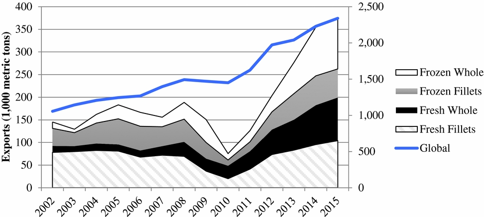
The global production of Atlantic salmon (Figure 1) shows a decline from 2008 to 2010, suggesting that other producing countries could not fully make up for the reduction in the Chilean output. This is also the main reason for the price increase during the same period, as discussed by Asche and Sikveland (Reference Asche and Sikveland2015) and Asche, Oglend, and Kleppe (Reference Asche, Oglend and Kleppe2017). In addition, as shown by Xie and Zhang (Reference Xie and Zhang2014), market shares in specific markets changed substantially. In particular, on the U.S. market, the market shares from countries other than Chile and Canada increased from 23% in 2007 to 45% in 2010 and went back down to 28% in 2012.
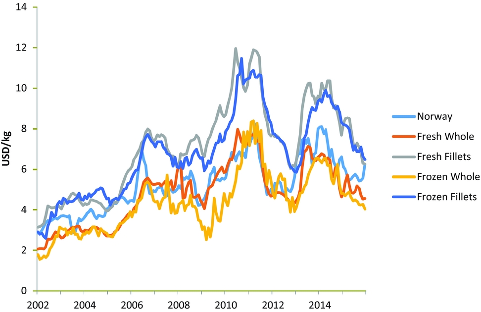
Figure 2 shows unit prices derived from the Chilean export statistics and converted to U.S. dollars (USD), as well as the Norwegian export price in USD. All prices follow a similar trend between 2002 and 2015, with the fresh and frozen fillets fetching clearly higher prices than the rest of the product forms. There is also a tendency for the frozen product forms to have a lower price than the fresh ones, although there is enough short-run variation in the prices for this not to always be the case. The figure also distinctly shows the peak in prices caused by the supply reduction from Chile in 2010. A similar peak can be noticed for the Norwegian price, an indication that Norwegian producers benefitted from the crisis in Chile in the form of higher prices.
Monthly Chilean Export Prices by Product Form and Norwegian Export Prices, 2002–2015 (sources: Chilean export statistics [unpublished data from SERNAPESCA, Santiago, Chile], 2016; Norwegian export statistics [unpublished data from Statistisk sentralbyrå, Oslo, Norway], 2016)
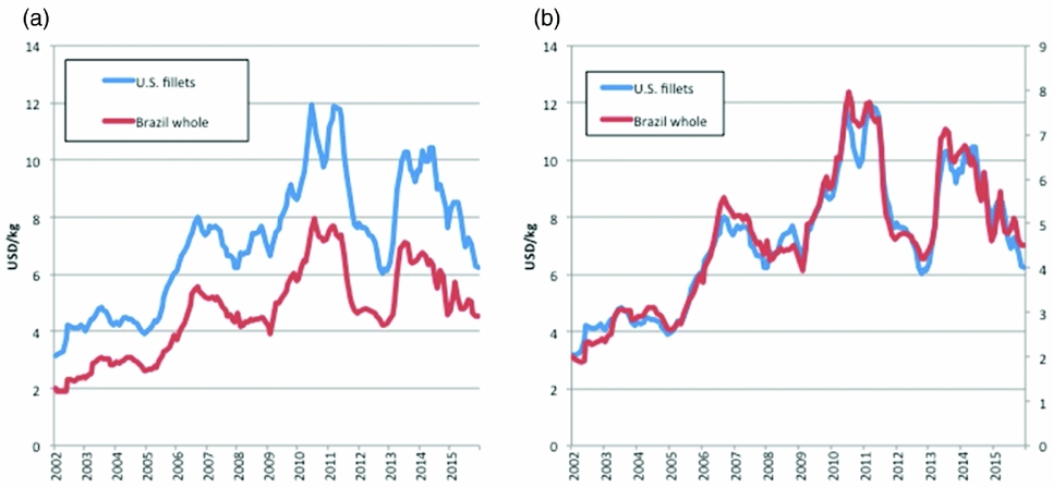
A key feature of the Chilean exports is that there is one main market for fresh fillets, as the United States receives more than 90% of this product form. Similarly, there is one main market for whole fresh salmon, and that is Brazil.Footnote 7 For frozen products, where perishability is more controlled, there is no dominant market, with products going to a number of countries in Europe and Asia in substantial quantities. In Figure 3, the export prices for fresh fillets to the United States and whole fresh to Brazil are shown in the left-hand panel, with the scale for the Brazilian price moved to the right-hand axis in the right-hand panel. The stable relationship between the two prices is clearly shown in the left-hand panel of Figure 3, with the fillet price to the United States at a premium and the strong comovement of the prices very clear in the right-hand panel. This provides a strong indication that the relative price is constant.
Monthly Chilean Export Prices of Fresh Fillets to the United States and Whole Fresh Salmon to Brazil (a) and the Same Series with Brazil Price Moved to the Right-Hand Axis (b) (source: Chilean export statistics [unpublished data from SERNAPESCA, Santiago, Chile], 2016)
This price development (Figure 3) occurs despite a very different development in quantities (Figure 4). The left-hand panel of Figure 4 shows the development in actual quantities, whereas the right-hand panel shows the shares. The development in the actual total quantity exported to the two markets is relatively similar to the aggregate data (Figure 1). Exports of whole salmon to Brazil were very limited in 2002, increased strongly in 2008 when small fish were harvested before showing symptoms of disease, remained at that export level throughout the crisis, and increased rapidly thereafter. The second panel shows how after 2008 the export share of whole salmon to Brazil increased relative to the fresh fillets to the United States, peaked at the height of the crisis in 2010, and then stabilized at a much higher level than prior to the outbreak. As shown in Figure 3, the relative price remained fairly constant throughout this period, with the change in export shares being only a response to the market opportunities faced by Chilean producers when the size composition of their fish changed.
Annual Chilean Export Quantities of Fresh Fillets to the United States and Whole Fresh Salmon to Brazil: Actual Quantities (a) and Shares (b) (source: Chilean export statistics [unpublished data from SERNAPESCA, Santiago, Chile], 2016)

The data series used in the analysis comprises 168 observations of monthly unit prices from Chilean and Norwegian exports, for the period January 2002 to December 2015. All prices were converted into USD for comparison.Footnote 8,Footnote 9 Before any econometric analysis can be conducted, the properties of the time series must be investigated. As the analysis is to be carried out using logarithms of the prices, augmented Dickey-Fuller (ADF) tests are first run.Footnote 10 The results are reported in Table 1, and, as expected given the general literature, all price series are nonstationary in levels, but stationary in first differences.
Unit Root Tests
Note: Asterisks (*, **) indicate statistical significance at the 5% level and the 1% level, respectively.
3. Methods
When conducting empirical analysis of market integration, the basic relationship to be investigated is given as follows:
 $$\begin{equation}
lnP_t^1 = \alpha + \beta lnP_t^2 + {e_t}.
\end{equation}$$
$$\begin{equation}
lnP_t^1 = \alpha + \beta lnP_t^2 + {e_t}.
\end{equation}$$
Here, Pit is the price observed for product i at time t, α captures differences in price level associated with transportation costs or quality differences, and et is the error term. If β = 0, there is no relationship between the two price series. If β = 1, then the relative prices are constant and the markets are fully integrated. This is also known as the law of one price (LOP). If 0 < β < 1, there is a relationship between prices that varies with the price level, indicating imperfect substitution.Footnote 11
When the price variables are nonstationary, the Johansen test is the most common tool (Asche, Bremnes, and Wessells, Reference Asche, Bremnes and Wessells1999). This is based on the following vector error correction model (ECM):
 $$\begin{equation}
\Delta {P_t} = \mathop \sum \limits_{i = 1}^{k - 1} {\Gamma _i}\Delta {P_{t - i}} + {\Gamma _k}{P_{t - k}} + \mu + {e_t},
\end{equation}$$
$$\begin{equation}
\Delta {P_t} = \mathop \sum \limits_{i = 1}^{k - 1} {\Gamma _i}\Delta {P_{t - i}} + {\Gamma _k}{P_{t - k}} + \mu + {e_t},
\end{equation}$$
where Γi is a matrix of parameters to be estimated, μ is a constant term, and the error term et is assumed to be indentically independently distributed with mean zero and variance W, et ~iid(0,W) (Johansen and Juselius, Reference Johansen and Juselius1990). The rank of Γk, r, indicates the number of stationary linear combinations, long-run relationships, or cointegrating vectors, in the vector containing the prices, Pt. If there are no linear combinations that are stationary (r = 0), then there are no cointegrating vectors. If the variables are stationary in levels, then the rank is equal to n (r = n), which would contradict the stationarity tests reported in Table 1. Johansen and Juselius (Reference Johansen and Juselius1990) provide a trace test that can be used to check for the number of cointegrating vectors (0 ≤ r ≤ n) in the system. If the price series are cointegrated, it is possible to factorize Γk = αβ', where both α and β′ are n × r matrices. The matrix β contains the r cointegrating vectors or long-run relationships, and the matrix α contains the speed of adjustment (or factor loadings).
Hypotheses on the α and β matrices can be investigated using likelihood ratio tests (Johansen and Juselius, Reference Johansen and Juselius1990). When the system contains two prices, there will be one cointegrating vector if there is market integration. In order to test if relative prices are constant, the restriction β' = (1, −1) is tested. If there are more than two prices in the system, there will be n − 1 cointegrating vectors and one stochastic trend if all products compete in the same market. Constant relative prices require that the parameters in each cointegrating vector sum up to zero (Asche, Bremnes, and Wessells, Reference Asche, Bremnes and Wessells1999). That is, in a system with four prices, there will be three cointegrating vectors if all goods are substitutes. To test the LOP, one test is whether the null hypothesis β1 = β2 = β3 = −1 in the matrix of cointegrating vectors:
 $$\begin{equation}
\beta = \left[
\begin{array}{l@{\quad}l@{\quad}l}
1 & 1& 1\\
\beta _1 & 0 & 0\\
0 & \beta _2 & 0\\
0 & 0 & \beta _3\end{array} \right].
\end{equation}$$
$$\begin{equation}
\beta = \left[
\begin{array}{l@{\quad}l@{\quad}l}
1 & 1& 1\\
\beta _1 & 0 & 0\\
0 & \beta _2 & 0\\
0 & 0 & \beta _3\end{array} \right].
\end{equation}$$
This matrix of cointegrating vectors illustrates that a system with n − 1 cointegrating vectors can always be normalized to n − 1 bivariate relationships, as noted by Johansen and Juselius (Reference Johansen and Juselius1994). Information with respect to weak exogeneity, or price leadership for a specific price, can be obtained by testing the restriction that parameters in the corresponding row of the α matrix are zero.
4. Empirical Results
The first step in the empirical analysis is to test for market integration between the export price of fresh fillets to the United States and whole fresh salmon to Brazil.Footnote 12 The results are reported in Table 2. The trace test in the third column indicates that the two prices are cointegrated. The LOP test in the fourth column indicates that this hypothesis cannot be rejected. Hence, these two products are a part of the same market with a constant relative price in the long run. This is, of course, not surprising given the price development shown in Figure 3. Finally, the weak exogeneity tests indicate that the price of fresh fillets to the United States leads the price of whole salmon to Brazil. The next step is to test for market integration for all four product forms exported from Chile. Table 3 reports these results. The trace test indicates that in this system with four prices there are three cointegrating vectors, and that the prices accordingly share the same stochastic trend. The LOP hypothesis cannot be rejected, and consequently, there is one well-integrated market being served by all Chilean salmon product forms. The weak exogeneity tests indicate that in this system too, fresh fillets are the leading price.
Market Integration Tests, Fresh Fillets to the United States and Whole Fresh Salmon to BrazilFootnote a
a P values in brackets.
Note: Asterisks (**) indicate statistical significance at the 1% level.
Market Integration Tests, Chilean Export PricesFootnote a
a P values in brackets.
Note: Asterisks (*, **) indicate statistical significance at the 5% level and the 1% level, respectively.
The final system to be estimated is the one where the Norwegian export price is introduced into the system with the four Chilean prices. The results are reported in Table 4. The trace test indicates four cointegrating vectors in this system of five prices, and that the LOP cannot be rejected. Therefore, there is one global salmon market, of which Chilean salmon is a part. More interestingly, the Norwegian price is found to be weakly exogenous. Hence, the price determination takes place outside of Chile, and Chilean producers are price takers in the global salmon market.
Market Integration Tests, Chilean and Norwegian Export PricesFootnote a
a P values in brackets.
Note: Asterisks (*, **) indicate statistical significance at the 5% level and the 1% level, respectively.
Although all investigated systems indicate a stable market integration relationship over the entire period, this will also be investigated by testing the relationships before and after the disease outbreak. This has to be done in several steps. First, as there are no tests available to test for a changed number of cointegration vectors in a system, cointegration is tested for using the data before March 2009 and after April 2009. These results, using the aggregate Chilean price and the Norwegian price, are reported in Table 5. The results are similar for both periods; there is one cointegrating vector, the LOP is not rejected, and the Norwegian price is exogenous. Given that the price series are cointegrated in both samples, the approach of Johansen, Mosconi, and Nielsen (Reference Johansen, Mosconi and Nielsen2000) can be used to test if deterministic components, in our case the constant term, have a structural break. Also with this specification, there is one cointegration vector and one common stochastic trend for the whole sample. A test for whether the structural break dummies are zero has a P value of 0.073, and the null hypothesis can accordingly not be rejected at a 5% level. Johansen, Mosconi, and Nielsen (Reference Johansen, Mosconi and Nielsen2000) note that hypothesis can be conducted on the slope parameters under the assumption of a given number of cointegration vectors. A test for a structural break in the cointegration relationship cannot reject the null hypothesis of no structural break with a P value of 0.133, which is not too surprising given that the LOP holds in both subsamples. Hence, the degree of market integration does not seem to be different before and after the disease outbreak.
Market Integration Tests, Chilean and Norwegian Export Prices before and after 2009Footnote a

a P values in brackets.
Note: Asterisks (*, **) indicate statistical significance at the 5% level and the 1% level, respectively.
5. Concluding Remarks
The Chilean disease shock caused by the ISA was sufficiently severe to increase global salmon prices substantially as other producers could not fully make up for the Chilean reduction in production. The disease shock also influenced product mix and trade patterns for Chilean exports. However, the shock did not lead to any segmentation of the salmon market. Our empirical results indicate a highly integrated market for all four Chilean product forms investigated, and that these are all well integrated into the global market. Moreover, the Norwegian price leads the Chilean prices, indicating that Chilean salmon prices are determined at the global market level. The lack of impact of the Chilean disease shock on price determination for salmon provides strong evidence of a highly integrated salmon market, where trade patterns shift to maintain the stable relative price. This is in contrast to some other markets for farmed fish, where fish size (Bjørndal and Guillen, Reference Bjørndal and Guillen2017a; Regnier and Bayramoglu, Reference Regnier and Bayramoglu2017) or quality (Bjørndal and Guillen, Reference Bjørndal and Guillen2017b; Norman-López and Asche, Reference Norman-López and Asche2008; Pincinato and Asche, Reference Pincinato and Asche2016; Rodríguez, Bande, and Villasante, Reference Rodríguez, Bande and Villasante2013) segments the market. However, our results support and strengthen the general conclusion for most seafood markets—that for the same and similar species, there exist well-integrated markets (e.g., Ankamah-Yeboah, Stål, and Nielsen, Reference Ankamah-Yeboah, Ståhl and Nielsen2017; Bronnmann, Ankamah-Yeboah, and Nielsen, Reference Bronnmann, Ankamah-Yeboah and Nielsen2016; Tveteras et al., Reference Tveteras, Asche, Bellemare, Smith, Guttormsen, Lem, Lien and Vannuccini2012; Vinuya, Reference Vinuya2007).
The high degree of market integration implies that Chilean salmon producers did not get any additional price increases during the disease crisis relative to other salmon producers. There is no evidence of an origin premium for Chilean salmon to partly compensate for the reduction in production. Rather, all salmon producers benefited to the same degree from the price increase, with the difference that the other producers did not have any reduction in quantity produced, only strong price incentives to increase it. The Chilean industry's response with respect to which markets were being served is also interesting. It is well known that different markets have different preferences with respect to fish size, and that price levels vary with size (Asche and Guttormsen, Reference Asche and Guttormsen2001). There is also evidence that earlier market shocks, such as antidumping tariffs, have led to changes in trade patterns (Asche, Reference Asche2001). It is therefore not surprising that Chilean producers responded to the disease crisis by changing the markets that were served. What is surprising is that a crisis became the time to develop new markets, as was the case for whole fresh salmon to Brazil. This is even more interesting when observing that the Brazilian market continues to be an important one in the aftermath of the crisis. This is a good example of demand growth by expanding the market's geographic size, one of the main strategies for demand growth for salmon (Brækkan and Tyholdt, Reference Brækkan and Tyholdt2014).


 Open access