1. Introduction

The realization nearly a decade ago that subglacial lake activity causes ice surface elevation changes that are detectable by satellite altimetry (Reference Gray, Joughin, Tulaczyk, Spikes, Bindschadler and JezekGray and others, 2005; Reference Wingham, Siegert, Shepherd and MuirWingham and others, 2006; Reference Fricker and ScambosFricker and others, 2007) has transformed our understanding of the Antarctic ice sheet’s subglacial water system. Prior to this discovery the major components of the subglacial hydrologic system were thought to be isolated stable lakes located primarily near ice divides (e.g. Reference Siegert, Carter, Tabacco, Popov and BlankenshipSiegert and others, 2005) and quasi-steady distributed water flow beneath the ice streams and outlet glaciers (Reference Engelhardt and KambEngelhardt and Kamb, 1997). We now understand that the hydrologic system is connected throughout (Reference WrightWright and others, 2012), with water travelling distances of hundreds of km in broad but well-defined channels on timescales of a few months (Reference Wingham, Siegert, Shepherd and MuirWingham and others, 2006; Reference Carter, Blankenship, Young, Peters, Holt and SiegertCarter and others, 2009a; Reference Flament, Berthier and RémyFlament and others, 2014). Water flow continues to the grounding line, providing a pathway for subglacial water to reach the Southern Ocean (Reference GoodwinGoodwin, 1988; Reference Fricker and ScambosFricker and others, 2007; Reference Carter and FrickerCarter and Fricker, 2012; Reference Le Brocq, Hubbard, Bentley and BamberLe Brocq and others, 2013) and contribute directly to sea-level rise. Glacier flow changes, especially glacier changes that strongly affect ice surface slope, can ‘activate’ subglacial water bodies and cause a drainage event (Reference Scambos, Berthier and ShumanScambos and others, 2011). The presence of water beneath an ice stream, and its action as a lubricant either between the ice and subglacial bed or between grains of a subglacial till, affects ice flow rates and thus continental ice flux (Reference KambKamb, 1987). Basal water systems may also serve to transport significant amounts of heat at the ice-sheet base (Reference Parizek, Alley and HulbeParizek and others, 2003; Reference Wolovick, Bell, Creyts and FrearsonWolovick and others, 2013). Understanding these systems is therefore crucial for ice-sheet modelling.

Surface deformation resulting from subglacial lake activity leads to anomalously large (>1 m a⁻¹) localized elevation changes: elevation gain over filling lakes (positive dh/ dt), and elevation loss (negative dh/ dt) over draining lakes; such signals have now been detected by several satellite instruments. The first demonstration of this used RADARSAT synthetic aperture radar data on Kamb Ice Stream, West Antarctica, over a single time interval (Reference Gray, Joughin, Tulaczyk, Spikes, Bindschadler and JezekGray and others, 2005). Satellite-radar-altimeter derived dh/ dt estimates for a longer time period (1995–2003) at four altimeter crossovers were attributed to linked draining and filling of subglacial lakes near Adventure Trench, East Antarctica (Reference Wingham, Siegert, Shepherd and MuirWingham and others, 2006). Repeat-track analysis of Ice, Cloud and land Elevation Satellite (ICESat) laser altimetry for the period 2003–06 identified a complex, active plumbing system involving linked reservoirs under the fast-flowing portions of three large West Antarctic ice streams (Whillans, Mercer and MacAyeal), and the dh /dt signals combined with areas from MODIS image differencing allowed for estimates of volume changes (Reference Fricker and ScambosFricker and others, 2007, Reference Fricker, Scambos, Carter, Davis, Haran and Joughin2010; Reference Fricker, Scambos, Bindschadler and PadmanFricker and Scambos, 2009). A continent-wide study by Reference Smith, Fricker, Joughin and TulaczykSmith and others (2009) used automated processing of ICESat data from 2003 to 2008 to produce an inventory of 124 lakes undergoing detectable dh/dt (‘active’ lakes), at locations different from those mapped with previous methods (e.g. Reference Siegert, Carter, Tabacco, Popov and BlankenshipSiegert and others, 2005; Reference Wright, Siegert, Brocq and GoreWright and Siegert, 2012); ten active lakes were identified in the Recovery catchment.

Recovery Ice Stream (previously called ‘Recovery Glacier’ (Reference Swithinbank, Brunk and SieversSwithinbank and others, 1988)) is Antarctica’s longest dynamic ice-flow feature, extending ~ 1000 km into the interior of the East Antarctic ice sheet (Reference Jezek, Farness, Carande, Wu and HamerJezek and others, 2003; Reference Rignot, Mouginot and ScheuchlRignot and others, 2011). It drains a large area of Dronning Maud Land, equivalent to 8% of the entire Antarctic ice sheet area, and provides 58% of the ice flux into the Filchner Ice Shelf (Reference Joughin and BamberJoughin and Bamber, 2005; Reference Joughin, Bamber, Scambos, Tulaczyk, Fahnestock and AyealJoughin and others, 2006). The Reference Smith, Fricker, Joughin and TulaczykSmith and others (2009) active lake inventory described ten active lakes under the main trunk of the lower Recovery Ice Stream and resolved the movement of subglacial water through this system for the period 2003–08 (see Fig. 1 for lake locations). Farther upstream, four large lakes were identified close to the Recovery Ice Stream onset area of fast flow, using both traverse and satellite data (Reference Bell, Studinger, Shuman, Fahnestock and JoughinBell and others, 2007; see Fig. 1 for lake locations). Aligned along a tectonic boundary and characterized by extensive very low-slope areas of the ice sheet, it is thought that these lakes are stable and are likely at a low stand (e.g. Reference LangleyLangley and others, 2011). Recovery Ice Stream is far from major research bases, and field expeditions have been limited to geologic exploration of the Shackleton Mountains (e.g. Reference Faure and MensingFaure and Mensing, 2010), one seismic and gravity traverse during the 1957 International Geophysical Year, and a US/Norwegian traverse over the upper lake system during the International Polar Year (IPY) 2008–09. The AGAP (Anarctica’s Gamburtsev Province) project (Reference BellBell and others, 2011) flew three exploratory flights over the two southern large lakes during the IPY (Reference LangleyLangley and others, 2014). NASA’s Operation IceBridge mission flew six flights in the Recovery region in October and November 2011 and November 2012 (see Fig. 1 for flight lines).

Fig. 1.

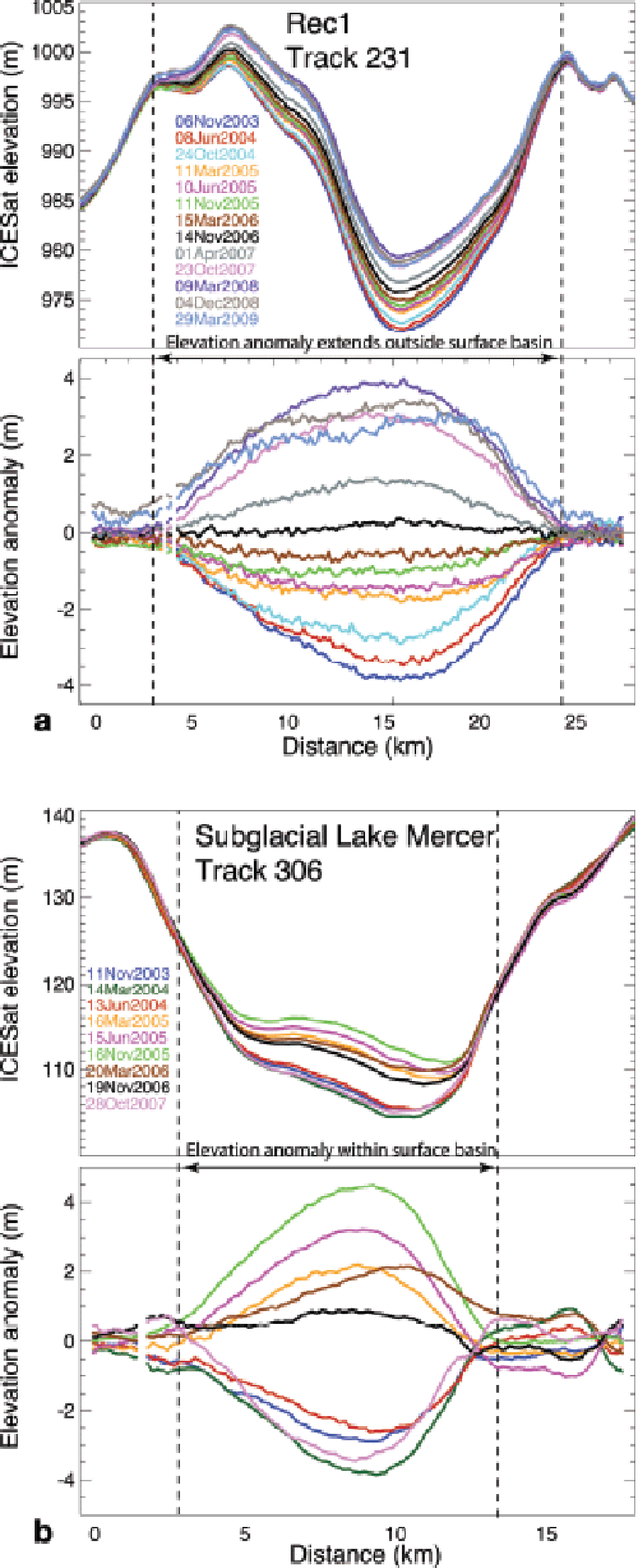
Main panel: MODIS Mosaic of Antarctica (MOA) over Recovery Ice Stream showing all known active and static lakes in the system, including Reference Bell, Studinger, Shuman, Fahnestock and JoughinBell and others (2007) lakes and Reference Smith, Fricker, Joughin and TulaczykSmith and others (2009) lakes and the locations of active subglacial lakes found in this study. ICESat reference tracks are shown as black thin lines with coloured line segments over lakes representing the total range of elevation during the ICESat period (2003–09); colour scale at top right. IceBridge flight lines for 2011 and 2012 are shown. The 2011 flights were F07 on 21 October 2011, which included ICESat track 404 across Rec2, and F16 on 7 November 2011 which flew along ICESat tracks 1297 and 97 (Rec1), 285 (Rec2), 305 (Rec3). The 2012 flight was on 18 October 2012, which included ICESat tracks 112 and 350 (Rec1), 335 and 82 (Rec2), 1302, 181 and 171. The segments where we compared Airborne Topographic Mapper (ATM) with ICESat data are labeled with the track number; the white ticks indicate the 50 km line segments shown in Figure 5. Upper inset left: volume change time series for the four main active Recovery Ice Stream lakes: ICESat observations 2003–09 (solid lines) and modelled time series (dashed lines). Lower inset left: water volume flux through the nine lakes of the active subglacial lake system over the ICESat period 2003–09; dark grey is water loss (flooding) and light grey is water gain (filling) at each lake. Lower inset right: study location in Antarctica.

In this study we combine repeat-track ICESat laser altimetry data (2003–09), IceBridge laser altimetry and radio-echo sounding (RES; 2011 and 2012) and MODIS image differencing (2009–11) to show the activity of the Recovery Ice Stream lake system from 2003 to 2012 and describe the topographic setting for these active lakes. We corroborate the extent of the subglacial drainage using an image-differencing method (Reference Bindschadler, Scambos, Choi and HaranBindschadler and others, 2010). We also estimate the hydropotential controlling the water flow and describe general constraints on the flow of water through the system. Using a subglacial water model, we simulate basal water distribution and subglacial lake filling rates, to test the consistency between the catchments and flow paths implied by our hydropotential surface and inferred lake volume change.

2. Data

3. Methods

3.1. Lake activity from ICESat repeat-track analysis

We analysed ICESat data following the repeat-track technique described by Reference Fricker and ScambosFricker and others (2007, Reference Fricker, Scambos, Carter, Davis, Haran and Joughin2010) and Reference Fricker, Scambos, Bindschadler and PadmanFricker and Scambos (2009). For each lake, we derive an average elevation for the entire lake at epochs that correspond to the centre of each ICESat campaign, in the following steps:

1. Calculated the elevation anomaly for each repeat (the difference of the elevation profile acquired during each campaign from the mean of all repeat profiles) for every track across each lake. We improved on the repeat-track technique used in previous studies (e.g. Reference Fricker and ScambosFricker and Scambosk 2009) by splitting the ~ 275 m wide swath of repeat tracks into narrower strips of tracks that repeat more closely (100–200 m), to reduce noise introduced by cross-track slope error (see Fig. 2).

2. Estimated the average anomaly for each repeat track to provide an elevation for each epoch for each track, referenced to the elevation at the first epoch.

3. For each epoch, we averaged the elevations from all tracks, using a weighted-average scheme described in Reference Fricker, Scambos, Carter, Davis, Haran and JoughinFricker and others (2010), where weights are equal to the length of the ‘on-lake’ track segment divided by the sum of all on-lake track segment lengths present in that epoch, to provide a single, lake-averaged elevation.

Fig. 2.

Improved ICESat analysis to reduce the effect of cross-track topography on ‘swath’ of repeat tracks for track 363 across Rec9 (see Fig. 1 for location). We improved on the repeat track technique by splitting the 275 m wide swath of repeat tracks into narrower strips of tracks that repeat closely (generally 100–200 m) to reduce the effect of (unknown) cross-track topography on the elevation anomaly, and treating them as independent tracks. In regions of rough topography, this technique improves the signal to noise ratio for those tracks whose ‘swaths’ of repeats are broad.

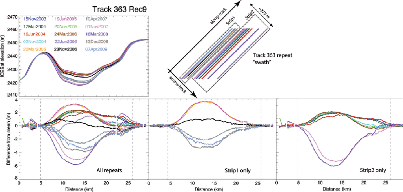
The resulting lake-averaged time series for each lake is the average of the elevation anomaly along each track, averaged over all tracks sampled during a campaign. We plotted the elevation anomalies on MOA and estimated the lake areas from these. The volume time series were obtained by multiplying the elevation time series by the estimated lake areas, assuming that the lake area remains constant at all stages of a lake fill–drain cycle.

3.4. Hydropotential from IceBridge radar ice thicknesses and Bedmap2

We used the IceBridge MCoRDS along with the Bedmap2 database (Reference FretwellFretwell and others, 2013) to construct a hydro-potential surface following the Reference ShreveShreve (1972) formulation:

(1)

where ρ _w and ρ _i are the densities of water (1000 kg m^–3) and ice (917 kg m^–3), respectively, z _b is the measured elevation of the ice base and h _i is the ice thickness (equal to z _s – z _b, with z _s being the measured elevation of the ice surface). Given this equation for governing basal pressure gradients of a thin liquid layer, surface elevation gradients are 11 times more significant than bed gradients for determining the direction of basal water flow. Bedrock gradients however, can locally exceed surface gradients by a factor of >11.

Although Bedmap2 represents the best bedrock map of Antarctica to date and has successfully assimilated a great variety of data sources including all IceBridge ice thickness and bedrock elevations from 2011 and earlier, a substantial degree of smoothing was applied to the input dataset for the Recovery Ice Stream region. In particular, features in the basal topography that would be important to our understanding of the flow of water in this region may have not been resolved. To take advantage of the high resolution of the IceBridge bed topography in places where it is available, we make the bed elevation of any 2.5 km × 2.5 km gridcell containing IceBridge measurements equal the average of all samples within it, and the bed elevation of points more than 7.5 km (~3 gridcells) distant from an IceBridge measurement equal to the Bedmap2 value. We then fit a two-dimensional bi-cubic spline to the region within 7.5 km of an IceBridge measurement, but not actually covered by IceBridge to preserve smoothness. The initial hydropotential was then obtained using Eqn (1) and the Bedmap2 surface elevation. We made further improvements to the hydropotential grid through ‘etching’ and ‘tuning’; both are described in detail in Appendix A.

4. Results

The combination of ICESat, IceBridge data and image differencing provided significant new information about the Recovery Ice Stream lakes, including the bedrock topography beneath them and how it controls the transport of water through the system. We present the bedrock topography results first (Section 4.1), describe the lake activity for the ICESat and IceBridge periods (Section 4.2) and then present the modelling results (Section 4.3).

4.1. Bedrock topography controls on Recovery subglacial hydrology

4.1.1. Bedrock topography and ice velocity

The gridded bedrock map from the IceBridge/Bedmap2 ice thickness data shows the basal morphology of Recovery Ice Stream (Fig. 3a). An elongated bedrock trough underlies the central trunk of Recovery Ice Stream. The ice stream is bisected into upper and lower troughs by a 500–1000 m high ridge located at ~ 17° W; the 500 km long lower segment is up to 2000 m deep and 40 km wide. Bounded by the Shackleton Range to its north, the lower trough has steep lateral margins (typical slope of 0.2–0.6), where total bedrock relief from the top of the Shackleton Range to the bottom of the Recovery trough approaches 4000 m. The upper segment is ~ 1500 m shallower and slightly wider. Ice thickness is 2500–3000 m over the lower trough and 3000– 3500 m in the upper trough. The high velocities in the main Recovery Ice Stream trunk are generally confined to the deep troughs (Reference Scheuchl, Mouginot and RignotScheuchl and others, 2012; Fig. 3b).

Fig. 3.

(a) Map of ice-base elevation for main trunk of Recovery Ice Stream derived from IceBridge ice thickness data and Bedmap2. (b) Ice surface velocity (from Reference Scheuchl, Mouginot and RignotScheuchl and others, 2012) with contours of hydropotential. In (a, b), the three IceBridge flight segments corresponding to the radargrams shown in Figure 5 are marked as yellow lines A–A′, B–B′, C–C′. The primary hydrologic flow path (solid line) leaves Rec1 and passes over a saddle in the Shackleton Range (Shackleton branch); secondary flowline follows the ice flow direction (Recovery branch). (c) Hydropotential and bed elevation along the primary flow path (solid lines) and secondary flow path (dashed lines). The primary flow path (Shackleton) has less of a hydropotential barrier than the path that follows the ice flow. Ice-base elevation map shows that Recovery Ice Stream is grounded in a trough. Location of suspected ‘freezeon’ of basal ice (see Fig. 4) is indicated.

Downstream of the main trunk a broad ridge, presumed to be a southern extension of Shackleton Range, rises at least 1000 m to its crest (–200 m to –700 m) (Fig. 3a). Close to the eastern edge of the Shackleton Range, as the lower trough rises towards the grounding line, the ice flow bifurcates (Fig. 3b; see also Figs 3c and 4). The western portion of the ice flow moves towards a narrow section of grounding line, widely accepted to be the Recovery Ice Stream grounding line. The eastern portion of the ice flow veers to the east up and over the elevated topography at the edge of the Shackleton Range. This ice goes afloat adjacent to the Slessor Glacier inflow. We refer to the southern limb as the ‘Recovery branch’ and the northern limb as the ‘Shackleton branch’ (Fig. 3b and c).

The grounding line is located on the downstream side of the ridge, >500 m below the crest; the grounding line depth is 1700 m at the location of maximum ice flux (Recovery branch) and 1000 m at our inferred location of subglacial discharge (Shackleton branch; Fig. 3a–c). This suggests that at present Recovery Ice Stream is mostly grounded on a prograde slope, with the deeper southern section occupying a local minimum in a trough; this trough is probably connected to the larger Crary Trough that lies beneath much of Filchner Ice Shelf. In contrast, Slessor Glacier to the north has a retrograde slope over ~ 100 km of its length, from the Crary Trough into a similarly deep lower-glacier trough, with no topographic barrier (Fig. 3).

4.1.2. Location of active subglacial lakes

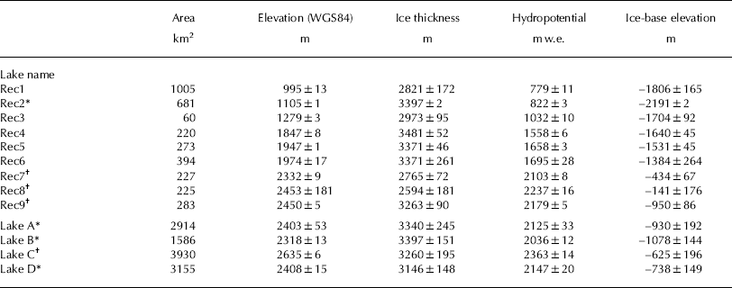
We identified nine active subglacial lakes in the Recovery system through our ICESat repeat-track analysis (Fig. 1; Table 1). Following the Reference Smith, Fricker, Joughin and TulaczykSmith and others (2009) convention, we named the lakes numerically starting from the most downstream lake and moving upstream (so the lake they called R _n , we call Recn). Two of the bodies that Reference Smith, Fricker, Joughin and TulaczykSmith and others (2009) identified as separate lakes (their R₁ and R₂), we found to be acting as a single larger lake (Rec1). Over one of the lakes (their R₇) identified by Reference Smith, Fricker, Joughin and TulaczykSmith and others (2009) we detected no signal in the surface elevation change above the noise (we use 0.5 m as the noise threshold); therefore, our lakes are named Rec1 to Rec9. These subglacial lakes are located at the base of the deep bedrock trough (Fig. 3a), and most are located towards its edges. Of the lower six lakes within the region covered by IceBridge, three (Rec6, Rec5 and Rec4) are in the upper trough above the steep bedrock ridge and three (Rec3, Rec2 and Rec1) are in the lower, deeper trough.

Table 1.

Statistics of the nine lakes in the Recovery system identified using 2003–09 ICESat data in this study, and the four lakes discovered by Reference Bell, Studinger, Shuman, Fahnestock and JoughinBell and others (2007). Unless otherwise indicated, values were obtained from mean and standard deviation of all IceBridge measurements of ice thickness and surface elevation occurring within the lake boundary

4.1.3. Hydropotential and subglacial water flow paths

Along the steep-sided trough in which Recovery Ice Stream sits, the hydropotential is predominately controlled by the bedrock topography (Fig. 3a and b). The lower six subglacial lakes are connected in a continuous chain, approximately following the ice-flow direction. Just downstream of the largest of the active lakes (Rec1), the primary hydrologic flow path diverges from the ice flowlines. This bifurcation in the hydrologic flow path is similar to the ice flow bifurcation (Figs 3b and 4). In contrast to ice flow, the majority of the water flux flows over a 1500 m saddle in the Shackleton Range before discharging into the Filchner Ice Shelf cavity near Slessor Glacier, >100 km north of where most ice discharge occurs. The ice stream crosses the southern extension of the Shackleton Range at its lowest topographic minimum. The steepening of the ice surface and the bifurcation in the subglacial water flow path both appear to be a consequence of the interaction between the ice flow and this southern subglacial extension of the Shackleton Range. Two radargrams acquired by the IceBridge radar in October 2011 show evidence of features not parallel to the bed, that may indicate accretion of basal water formed as water travels up and over the saddle in Shackleton Range and freezes into the ice-stream base (Fig. 4).

Fig. 4.

Flow bifurcation region downstream of Rec1. Top right is a location map showing lakes, hydrologic flow paths, and contours of ice surface elevation (interval 250 m; note steepening of ice surface near grounding line); rectangle shows the area covered by left panels. Left panels (from top to bottom): MOA showing the locations of the two predicted hydrologic flow paths (Shackleton flow path and the Recovery flow path; dashed and solid yellow lines), the location of segments D–D′ and E–E′ of IceBridge flight on 29 October 2011, and the grounding line; ice-base topography highlighting bedrock ridge crossed by the Shackleton flow path (solid yellow line); ice surface velocity (Reference Rignot, Mouginot and ScheuchlRignot and others, 2011); and ice surface velocity difference between 2009 and 1997 (Reference Scheuchl, Mouginot and RignotScheuchl and others, 2012). The panels at middle and bottom right are radargrams acquired by IceBridge radar along segments D–D′ and E–E′ (location shown on map figures). Middle: radargram oriented parallel to ice flow near suspected region of accreted ice, showing the stoss face of the Shackelton range and structural deformation in the overlying ice, related to ice flow. Bottom: radargram from the IceBridge radar along segment E–E′, showing features that are not parallel to the bed that may indicate accretion of basal water formed as water travels up and over the saddle in the Shackleton Range and freezes into the ice-stream base. Note the closeness of the internal layers to the ice base on either side of the upwarping, and the absence of layering in the lower part of the upwarped region.

4.2. Activity of Recovery Lakes

There are various sources of uncertainty in the volume estimates derived from our combined ICESat repeat-track analysis and MODIS analysis: (1) the actual error in the ICESat averaged along-track measurement; (2) inadequate sampling of the lakes by the ICESat tracks; and (3) the error in the lake area. Previous studies have adopted percentage errors for their volume estimates (20% (Reference Fricker, Scambos, Carter, Davis, Haran and JoughinFricker and others, 2010) and 50% (Reference Smith, Fricker, Joughin and TulaczykSmith and others, 2009)); here we assign an uncertainty of 25% to each volume estimate.

4.2.1. ICESat period 2003–09

Our ICESat repeat-track analysis of elevation change enabled us to produce a volume time series for the nine active lakes (Rec1–Rec9; Fig. 1 inset). We discuss the elevation change, volume change and estimated water flux of the nine lakes, starting at the most upstream lake and moving down-glacier. We then compare the estimated water flux with the modelled water flux.

The most upstream active lake is Rec9, located ~ 50 km downslope of the large lakes A and B. Our newly resolved area is ~ 282 km², which is substantially smaller than estimated by Reference Smith, Fricker, Joughin and TulaczykSmith and others (2009) (~728 km²). Our altimetry-defined lake margin closely resembles the lake extent mapped by Reference LangleyLangley and others (2011), using RES measurements of ice thickness and basal reflectivity. This suggests that lake shorelines determined using a combination of MODIS and ICESat (e.g. Reference Fricker, Scambos, Bindschadler and PadmanFricker and others, 2007) are more precise and consistent with RES than those determined by laser altimetry alone (e.g. Reference Smith, Fricker, Joughin and TulaczykSmith and others, 2009). Our ICESat analysis showed that the surface of Rec9 subsided by 0.47 m between November 2003 and February 2006, which converts to 0.13 km³ of water at a maximum rate of 4 m³ s⁻¹. Between then and the end of the observation period in 2009, Rec9 appears to have had no significant activity.

Lakes Rec8 (`225 km²) and Rec7 (~227 km²) are located in the western branch of Recovery Ice Stream 100 km downslope of large lakes C and D. Both Rec8 and Rec7 were filling between November 2003 and March 2004 at rates of 2.9 m³ s⁻¹ for Rec8 and 0.6 m³ s⁻¹ for Rec7. They began draining within 6 months of each other. Rec7 started draining first in March 2004, decreasing in elevation an average of 1.5 m, consistent with a volume decrease of 0.33 km³ at an average rate of 2.1 m³ s⁻¹ and peaking at 3.6 m³ s⁻¹ between November 2004 and March 2005. Rec8 began draining in October 2004. The average elevation over the lake decreased by 2.4 m between March 2004 and March 2008, resulting in a volume loss of 0.57 km³ at an average rate of 4.6 m³ s⁻¹, peaking at 12.6 m³ s⁻¹ between October 2006 and March 2007. As the volume loss rate for Rec8 reached a maximum, volume loss for Rec7 temporarily halted. When drainage of Rec8 had ceased by March 2008, and filling began again at a rate of 0.6 m³ s⁻¹ through the end of the ICESat observation period, Rec7 resumed draining at a rate of 3.1 m³ s⁻¹. If the two lakes are connected, then input of water from Rec8 may have been enough to offset ongoing volume loss at Rec7 between March 2006 and March 2007. The lack of ice thickness data in this region, however, does not allow us to determine this conclusively.

Rec6 (~394 km²) occupies one of the deeper parts of the upper Recovery trough. ICESat repeat-track analysis showed that the ice surface over Rec6 increased 0.7 m in the early portion of the ICESat record (November 2003 to March 2005); then from mid-2006 until the end of the mission in late 2009, the surface elevation decreased by a total of 7.8 m. The increase in elevation from November 2003 to March 2005 could have resulted from an influx of water from Rec9, which was draining during this interval. Drainage of Rec6 began in March 2005, but outflow was initially fairly low, with most volume loss occurring between 2006 and 2009. The elevation decrease during this interval is equivalent to a drainage rate of ~ 30 m³ s⁻¹, and it peaked at 56 m³ s⁻¹. The total volume lost from Rec6 during the ICESat observation period is ~ 3 km³.

Downstream of Rec6 are two smaller lakes Rec4 (220 km²) and Rec5 (273 km²). Early in the ICESat observation period the elevation of the ice surface over each of these two lakes increased by 1.5 and 1.1 m respectively between 2003 and early 2007. The majority of uplift coincided with the drainage of Rec6. Together the two lakes increased in volume by 0.33 km³ at a rate of 6.3 m³ s⁻¹. From early 2007 onward, the ice surface over these two lakes dropped, with Rec4 declining by 0.8 m and Rec5 declining by 0.3 m, for a total volume loss of 0.2 km³, which represents a water outflow of 3.7 m³ s⁻¹.

Three lakes are located downstream of the ridge that separates the upper and lower trough, one small (Rec3) and two large (Rec2 and Rec1). Rec3 is located along the western/southern margin of the ice stream, 30 km downstream of the ridge. This small (60 km²) lake was crossed by two ICESat tracks, which showed only a small (<1 m) elevation decrease during the ICESat observation period. During this period the total range in observed elevation change is only ~ 1.2 m averaged across the whole lake, with a maximum range of 2.4 m near the lake’s center. The decrease in surface elevation over Rec3 indicates a minimum volume change of 0.07 km³ and a water flux of 0.57 m³ s⁻¹.

The upstream large active lake (~681 km²) is Rec2 located near the northern margin of the ice stream. Between November 2003 and November 2005, no significant elevation changes were detected by ICESat; then, between March 2006 and March 2007, the ice surface increased by a total elevation of ~ 4 m. This elevation increase requires a volume change of 1.0 km³ and an influx of water at 35 m³ s⁻¹. The increase in Rec2 elevation is temporally coincident with the decreasing ice surface elevation of Rec6, and we interpret this as influx of water from Rec6. During the later part of the ICESat period, between March 2007 and November 2009, the ice surface over Rec2 dropped 1.1 m, representing a volume change of ~ 0.3 km³.

Rec1 is the largest active lake in the Recovery system (~1005 km²), stretching the full width of the ice stream, and located close to where the basal hydrologic path and the ice flow bifurcate. ICESat observations show that the elevation of the lake increased throughout most of the mission; from the beginning of the mission until September 2008, the average elevation over Rec1 increased by ~ 0.76 m a⁻¹, with a resultant total elevation increase of 3.7 m, representing a volume of ~ 4.5 km³. From September 2008 through the end of the ICESat mission, elevation remained constant or decreased slightly, and the volume in November 2009 was 0.6 km³ below the September 2008 maximum. We interpret the associated total volume increase of 3.7 km³ over 5 years (2003–08) as ongoing filling of the lake (Fig. 1). The elevation change would require an influx of water at 24.1 m³ s⁻¹ between 2006 and 2008, which is nearly twice the inflow between 2003 and 2006. The subsequent drainage discharged at a minimum of 18.8 m³ s⁻¹ to points downstream.

Considering the active lake system as a whole, the observed elevation and volume changes indicate that most of the ICESat period (2003–08) was dominated by surface lowering over two mid-glacier lakes (Rec6 and Rec9) and surface inflation over the lower two lakes (Rec1 and Rec2; Fig. 1 inset). We interpret surface lowering at Rec9 as water loss via a flooding event that began before 2003; the water travelled 150–200 km downstream toward Rec6, which filled until 2005 and then began to drain. In 2006, 8–12 months later, the elevation increased over Rec2, which we interpret as infilling with subglacial water which travelled a distance of ~ 350 km from Rec6. About 6 months later in 2006 the rate of ice surface inflation over Rec1 (another ~ 50 km downstream) increased, which we also interpret as a response to the draining of Rec6. As Rec2 then began to drain in late 2007, the filling rate of Rec1 increased, until the onset of surface lowering of Rec1 in 2008. Since it is the lowest lake in the system before the grounding line, water from Rec1 flows presumably to the cavity under the Filchner Ice Shelf. We interpret this event as a cascading flood from Rec9 to Rec6, then to Rec2 and then to Rec1, and then to the ocean; a total distance of ~ 800 km. The last year of the ICESat period (2008–09) was characterized by little change in the upper lakes and small elevation changes over the lower two lakes, which we interpret as slow drainage.

4.2.2. Post-ICESat mission 2009–12

The IceBridge lines provided new topographic information for the six lowest lakes in the Recovery Catchment (Rec1 to Rec6). The surveys covered ~ 500 km of the 800 km long path that the cascading flood travelled along. The IceBridge altimetry data along ICESat tracks over Rec3, Rec2 and Rec1 enabled us to extend our record of changes in elevation and volume over the lakes in the lower trough, but the upper trough lakes (where the IceBridge lines were sparse and not parallel to earlier ICESat profiles) could not be extended.

In 2011, IceBridge overflew ICESat track 305 over Rec3. The IceBridge radar revealed a 400 m deep topographic low below the segment of the ICESat track that corresponds to Rec3 (Fig. 5a). Comparison of the ATM elevation profile with ICESat elevations indicated a ~ 10 m subsidence of the ice surface between 2009 and 2011 (Fig. 5a), across the same ~ 10 km section where ICESat data revealed only small oscillatory elevation changes in 2003–09. This elevation change is of a similar magnitude to a change that occurred between 2003 and 2006 at Subglacial Lake Engelhardt, detected by ICESat and image differencing (Reference Fricker, Scambos, Bindschadler and PadmanFricker and others, 2007). However, here it occurs over significantly thicker ice, making the inferred lake margin less sharp in both the difference image and the elevation profiles. MODIS image differencing between 2009 and 2011 (Fig. 6, right panels) shows evidence of surface elevation change in the same location, spanning a similar range to the ICESat vs IceBridge-defined region of elevation change, and yielding a difference structure compatible with the structure of the profile difference. The difference image is less distinct than the Subglacial Lake Engelhardt difference image (Reference Fricker, Scambos, Bindschadler and PadmanFricker and others, 2007), however, because of the thicker (and colder, stiffer) ice.

Fig. 5.

IceBridge radargrams (unannotated at left) for three ICESat tracks that cross the lower three Recovery lakes: (a) track 305 Rec3; (b) track 285 Rec2; and (c) track 1297 Rec1. On each annotated radargram, the coloured lines towards the top are the surface elevation profiles from the ICESat repeats that were within 1 km of the IceBridge line (repeat dates at right in corresponding colours), and the white line is the IceBridge ATM surface elevation. The central line is the bed elevation picked from the radargram, and the bottom line is the hydropotential.

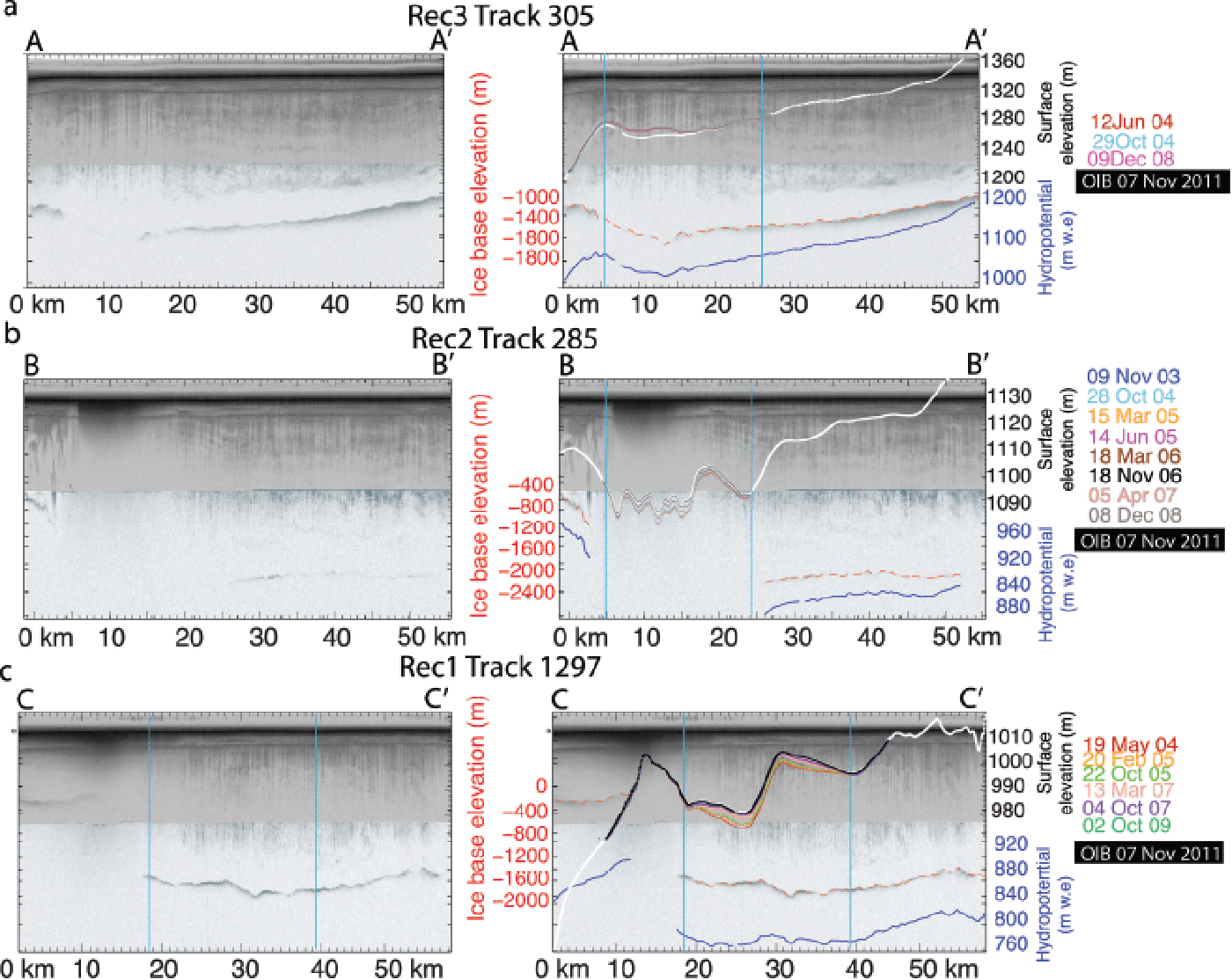
Rec2 is located in a deep subglacial basin along the eastern margin of Recovery Ice Stream and is covered with thick (~3500 m) ice (Fig. 5b). In this region, the trough bends, RAMP Ice Stream enters to the west and the ice stream is heavily crevassed. The combination of thick ice and heavy crevassing makes it a challenging radar environment, and the IceBridge RES instrument was unable to acquire a basal return over the lake (Fig. 5b).

IceBridge flew along ICESat tracks that cross Rec2 in both 2011 and 2012, overflying track 285 in November 2011 and tracks 335 and 82 in October 2012. Between 2008 and 2011 there was a ~ 1 m uplift over Rec2 (track 285). In contrast, the comparison of the ICESat and IceBridge 2012 elevations (tracks 335 and 82) showed an elevation drop of 3 m relative to the mean 2011 elevation (Fig. 5b), which we interpret as a drainage event. This suggests that Rec2 reached its maximum volume between November 2011 and October 2012.

In contrast to Rec2 and Rec3, Rec1 extends diagonally over 70 km across the full width of the Recovery Trough. The IceBridge RES ice thickness data revealed that the ice here is thinner (~2500–2900 m) and the trough is more symmetric. All three radar profiles crossing Rec1 have 2–3 km long segments of hydraulically flat bed that appears brighter and more consistently reflective than its surroundings, suggesting the presence of water (Reference Wolovick, Bell, Creyts and FrearsonWolovick and others, 2013). The RES data also revealed that a 300 m step in the ice-base topography coincided with the location of the maximum elevation anomaly from ICESat for the 2003–09 period (Fig. 5c) and a ~ 30 m step in the surface topography of the opposite slope. Although the hydropotential along with the elevation change observations indicate that the ice is in flotation over the entire structure, the mechanism for creating and maintaining such a steep thickness gradient in floating ice is unclear.

Rec1 was surveyed by IceBridge both in 2011 and 2012, along five ICESat tracks (2011: tracks 112, 1297 and 97; 2012: 112, 335 and 350). When the November 2011 IceBridge altimetry data were compared with the October 2009 ICESat data, there was no detectable elevation change along the repeats of tracks 97 and 1297 (Fig. 5c). The absence of elevation change between October 2009 and November 2011 was confirmed by MODIS image differ-encing for the same period (Fig. 5, left panels). Similar to Rec2, a distinct elevation change was detected when the November 2012 IceBridge altimetry was compared with the November 2009 ICESat data: between ICESat observations in November 2009 and the first IceBridge overflight in October 2012 there was an elevation drop of ~ 2 m (too small to detect with image differencing) along tracks 335 and 350. The elevation change between the two IceBridge observations indicates the lake started to drain between November 2011 and October 2012. The surface elevation in 2012 was still 5 m above the elevation observed at the start of the ICESat mission (October 2003). If the system was returning to its early ICESat state, then we infer that the drainage event was ongoing during the 2012 IceBridge survey.

4.3. Modelled water flux over the ICESat period 2003–09

We modelled the water fluxes necessary to reproduce the observed elevation changes during the 6 year ICESat period, with the goal of matching the observed filling rates of the two large lower lakes (Rec1 and Rec2). We used a relatively modest value for catchment-wide basal melt (0.7 mm a⁻¹), and allowed the large lakes (A–D) to be filling the entire time. Our water budget model predicted that the large upper lakes received ~ 7.7 m³ s⁻¹, 46% of the total meltwater budget produced in the Recovery catchment (area 869 km²). At these inflow rates, surface uplift on these large lakes would be below the ICESat detection limit. Regional basal melt is sufficient to support the water flux through the active lakes without input from the large lakes upstream (Reference Bell, Studinger, Shuman, Fahnestock and JoughinBell and others, 2007; Reference LangleyLangley and others, 2011).

Our modelling was the most successful for the lower six lakes, where there are sufficient ice thickness data; lack of ice thickness data, necessary for determining flow routing, in areas of steep basal topography as has been observed elsewhere in our study area, limited the ability of our model to reproduce the filling rates of the upper three active lakes (Rec7, Rec8 and Rec9), where the ice and bed topography used was based primarily on a gravity model (Reference FretwellFretwell and others, 2013).

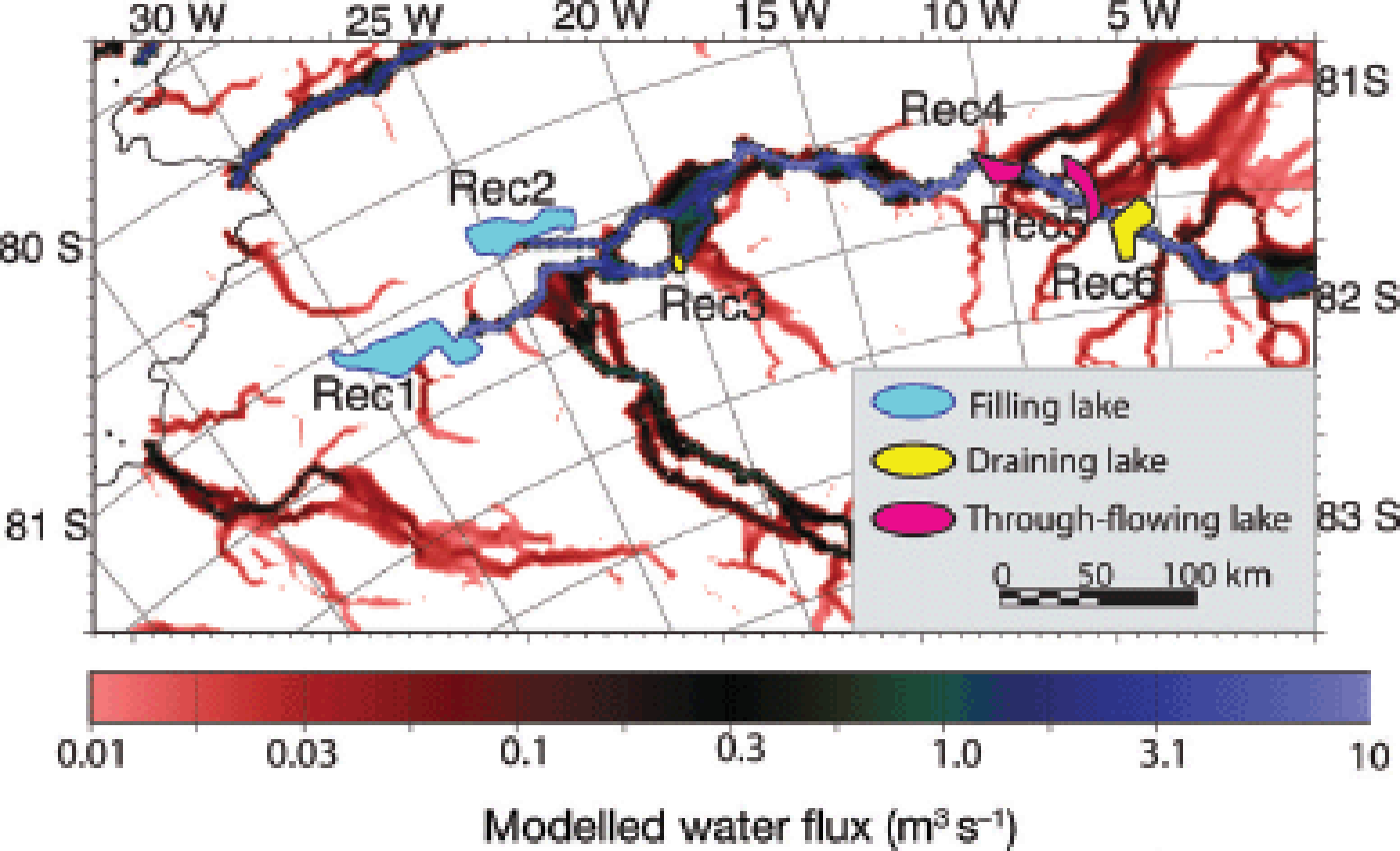
Our model suggests that volume is conserved during a cascading flood between lakes Rec9, Rec6, Rec2 and Rec1, with lakes Rec5, Rec4 and Rec3 acting as through-flowing features at this time. This suggests that Rec7 and Rec8 may be connected to one another; however, further interpretation is not possible due to the lack of data. A snapshot of the model for the period March–June 2006 shows water passing from Rec6 to Rec2 and then Rec1 (Fig. 7). An animation of the model is shown in Supplementary Movie S1 (in http://www. igsoc.org/hyperlink/14j063.gif)

Our model results suggest that Rec6 receives water from both Rec9 and the Rec7/Rec8 pair. For Rec6 the modelled filling rate is 8.1 m³ s⁻¹ between November 2003 and March 2005 (2.7 m³ s⁻¹ from the drainage of Rec9 and 1.1 m³ s⁻¹ from lakes Rec7 and Rec8). Given the 25% uncertainty (±1.6 m³ s⁻¹) for the observed volume change rate of 6.5 m³ s⁻¹, we considered the agreement between the modeled results and the observations to be reasonable. The filling and draining cycle of Rec6 regulates lake activity downstream: when Rec6 drains, water fluxes downstream increase by over an order of magnitude.

Fig. 6.

MODIS images (top) and difference images (bottom) spanning the IceBridge and ICESat epochs for two lakes: Rec1 (left panels) and Rec3 (right panels). Top left: a sub-scene from the MOA2009 image mosaic (Reference Haran, Bohlander, Scambos and FahnestockHaran and others, 2005). Bottom left: 2011–2009 MODIS difference image shows a smooth residual surface indicating no significant topographic changes in the lower glacier or over the lake outline. Top right: MODIS mosaic image of Rec3 subglacial lake area. Bottom right: 2011–2008 difference image shows a significant change in topography. Illumination of the images (and therefore of the residual representation of the change in the difference image) is from the right. The dark region on the right side of the Rec3 lake outline in its difference image, and bright patches on the left side, indicate changes in slope that are consistent with a multi-meter elevation loss at some time in the 2009–11 interval.

Fig. 7.

Snapshot of subglacial water model for one time step showing major flooding event from Rec6 to Rec3 and Rec1; the evolution of the flood for the entire ICESat period 2003–09 is animated in Supplementary Movie S1, online at http://www.igsoc.org/hyperlink/14j063.gif.

The estimated volume changes of Rec5 and Rec4 (<10 m³ s⁻¹ for each), are relatively small compared to that calculated for Rec6 (up to 60 m³ s⁻¹); the estimated volume for these two lakes reached a maximum in 2006/07, approximately coinciding with maximum discharge from Rec6 (Fig. 1, lower left inset). The subsequent rapid subsidence of Rec5 and Rec4 and the low total volume change undergone by these two lakes leads us to propose that these features swell only temporarily during times of high through-flow, instead of acting as substantial water storage features that impound water for a long period. Similar features have been observed on the lower Whillans/Mercer ice streams (Reference Carter, Fricker and SiegfriedCarter and others, 2013).

Rec3 exhibited even smaller volume changes than Rec5 and Rec4 (estimated <5 m³ s⁻¹), and it behaved differently to Rec5 and Rec4. There was a small filling event between November 2003 and March 2004, but the model was unable to accurately reproduce the observed filling rate, being too low by a factor of two. Since Rec6 was filling during this period, we could not test for a connection between Rec3 and Rec6. Between March 2005 and June 2009, when Rec5 and Rec4 were filling and draining (Fig. 1), Rec3 underwent a small draining event, i.e. there was no correlated activity between Rec3 and Rec5–Rec4. This also meant that the only way to treat it in the model during that time was as a source of water. In our model the flow path diverged upstream of Rec3, directing only about half of the water coming from the upstream lakes towards Rec3, and the rest towards Rec2 (Fig. 7). Combined with the lack of correlated activity between Rec3 and the Rec4–Rec5–Rec6 chain, this leads us to suggest that Rec3 is not hydrologically connected to those lakes and instead the water that flows into it is more locally derived. Furthermore, it is likely that our assumed uniform melt rate of 0.7 mm a⁻¹ is too low for Rec3’s catchment, given the evidence for enhanced shear heating (Reference Joughin, Bamber, Scambos, Tulaczyk, Fahnestock and AyealJoughin and others, 2006), suggesting that there are higher melt rates immediately upstream.

Rec1 and Rec2 are the only two water bodies downstream of Rec6 with enough storage capacity to truly test whether water is conserved within the system. When the model is tuned to partition equally between a route supplying Rec2 and one bypassing it directly toward Rec1, then the volume for the whole system is conserved, and the model reproduced the observed increase in inflation rate of Rec1 during the drainage of Rec2.

5. Discussion

The IceBridge ice thickness data have confirmed a deep subglacial channel (Fig. 3a), first suggested by Reference Joughin, Bamber, Scambos, Tulaczyk, Fahnestock and AyealJoughin and others (2006) from modelling, later inferred by Reference LangleyLe Brocq and others (2008) through surface observations, and partially resolved in Bedmap2 data (Reference FretwellFretwell and others, 2013). The channel is almost 1000 km long and >2000 m deep, making it the one of the longest mapped subglacial troughs under either ice sheet, comparable in length to the mega-canyons recently reported in Greenland (Reference Bamber, Siegert, Griggs, Marshall and SpadaBamber and others, 2013) and the Ellsworth Highlands of Antarctica (Reference RossRoss and others, 2014). The large subglacial trough contains the main trunk of Recovery Ice Stream, which sits ~ 1500–2200 m below sea level. Most of the nine active lakes detected with ICESat data are located at the edges of the subglacial trough. Inversion studies performed by Reference Joughin, Bamber, Scambos, Tulaczyk, Fahnestock and AyealJoughin and others (2006) proposed that beneath Recovery Ice Stream is a large amount of wet, deformable subglacial sediment/till. Although the fact that it sits below sea level would suggest that this ice stream might become sensitive to oceanic forcing, the ridge separating this main trough from the grounding line provides a level of protection that does not appear to exist for neighboring ice streams such as Slessor, Support Force, and Foundation or Möller (Reference RossRoss and others, 2012). A recent oceanographic modelling study predicted that the area of the Filchner Ice Shelf just in front of Recovery Ice Stream would be susceptible to intrusions of warmer water at the grounding line by 2075 (Reference Hellmer, Kauker, Timmermann, Determann and RaeHellmer and others, 2012). Given the presence of the bedrock ridge between Recovery Ice Stream grounding line and the main ice-stream trunk, its response to thermal oceanic forcing may be markedly different to neighboring ice streams, exhibiting substantially greater stability.

Our lake activity time series derived from ICESat observations for the period 2003–09 (Fig. 1) provides clear evidence that the main Recovery Ice Stream lakes are interconnected, with drainage events in upstream lakes leading to filling events downstream (Reference Smith, Fricker, Joughin and TulaczykSmith and others, 2009). The flow paths derived from our subglacial water modelling combined with our data show that for the largest detected drainage event, water was inferred to move ~ 800 km from Rec9 to the ocean; this is the longest distance that subglacial water has been inferred to flow under the East Antarctic ice sheet (the next longest being ~ 290 km in Adventure Trench (Reference Wingham, Siegert, Shepherd and MuirWingham and others, 2006)). We have shown that the water budget for these lakes balances for the ICESat period 2003–09 and is reproduced by a simple model that assumes 0.7 mm a⁻¹ melting over the entire glacier catchment. It is also of interest that for two of the lakes in our study (Rec8 and Rec3), the rate of volume loss decreased when a lake upstream was supplying additional water. This would indicate that there is some mechanism that limits the maximum rate of outflow at any given time, further supporting the at least ephemeral presence of conduits (as inferred by Reference Schroeder, Blankenship and YoungSchroeder and others, 2013). Additionally two lakes inflated when through-flow was high, but subsided thereafter, similar to behavior observed at Whillans Ice Stream (Reference Carter, Fricker and SiegfriedCarter and others, 2013). Given this is the second occurrence of such features in a system, it is likely that a number of water bodies included in the Reference Smith, Fricker, Joughin and TulaczykSmith and others (2009) inventory may be of a similar nature. Other water systems may become more hydrologically balanced once such features are better accounted for.

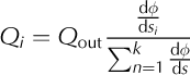
The scale of the Recovery hydrologic system is comparable to that of the Whillans/Mercer subglacial water system. However, the elevation anomalies observed over the Recovery lakes are qualitatively different to those observed over the Whillans/Mercer lakes (Reference Fricker, Scambos, Bindschadler and PadmanFricker and others, 2007; Reference Fricker, Scambos, Carter, Davis, Haran and JoughinFricker and Scambos, 2009). On the lower Whillans/Mercer, the elevation anomalies are confined to the bottom of surface topographic basins (Fig. 8), which implies that the water movement is controlled by surface elevation. The lower Whillans/Mercer region is an ice plain that is hydrologically flat with a slope of 0.0001; this hydrologic flatness makes the Whillans Ice Plain akin to a river delta. It has been shown that small changes in surface elevation can change the hydrologic potential and lead to complete reorganization of the Whillans subglacial water system through flow switching (Reference Carter, Fricker and SiegfriedCarter and others, 2013). On Recovery Ice Stream, however, bed elevation gradients often exceed surface elevation gradients by more than the critical factor of ~ 11. ICESat elevation anomalies extend across the entire topographic basin, including the sides, and then up to several km outside the basins (Fig. 8). This suggests that the hydropotential is more controlled by the deep bedrock basin in which the glacier sits, and less by surface topography relative to the Whillans systems. Because the bedrock is dominant in controlling the sub-glacial flow in this case, we propose that the Recovery Ice Stream subglacial system is more stable than the Whillans/Mercer system. This implies that a much greater change in ice thickness would be required before any major change in water-flow routing could take place in the Recovery system (as described in Reference Carter, Fricker and SiegfriedCarter and others (2013) for the Whillans/Mercer system). This, combined with the present-day grounding of Recovery Ice Stream at the bottom of the Crary Trough, implies that the ice geometry and subglacial water system have changed only gradually over the past several centuries (as compared to some of the relatively abrupt changes inferred for the Siple Coast (e.g. Reference Hulbe and FahnestockHulbe and Fahnestock, 2007)).

Fig. 8.

Typical ICESat elevation anomalies along ICESat tracks that cross subglacial lakes on (a) Recovery Ice Stream and (b) Mercer Ice Stream, showing the different extent of the elevation anomalies with respect to the surface topography. See Figure 1 inset map for location of Mercer Ice Stream in West Antarctica.

Our results point to a strong need for long (preferably decadal), continuous time series if we hope to understand lake activity and evolution for complex subglacial systems. Activity observed during the ICESat mission (2003–09), which is short compared to typical lake cycles, is not necessarily representative of longer-term behavior (Reference Siegfried, Fricker, Roberts, Scambos and TulaczykSiegfried and others, 2014). For example, Rec3 underwent very little activity over the ICESat period, yet experienced a very large negative elevation change between 2009 and 2011. It has been shown that it is possible to extend the time series using CryoSat-2 data (Reference Siegfried, Fricker, Roberts, Scambos and TulaczykSiegfried and others, 2014); however, in the Recovery Ice Stream region the synthetic aperture radar interferometric (SARIn) mode mask ends at Rec1, i.e. there are no SARIn mode data over the main Recovery Ice Stream lakes. The low-resolution mode (LRM) is a conventional radar altimeter akin to Envisat’s RA-2, and we have demonstrated on MacAyeal Ice Stream that this instrument cannot retrieve accurate data over subglacial lakes on ice streams due to the topography that is rough at length scales on the order of the altimeter pulse-limited footprint (Reference Fricker, Scambos, Carter, Davis, Haran and JoughinFricker and others, 2010).

An outstanding question is whether subglacial lakes affect ice dynamics. Water and wet sediments play an important role in determining the rate of ice-stream flow and in triggering changes in flow rates over short timescales (Reference Hulbe and FahnestockHulbe and Fahnestock, 2007; Reference Peters, Anandakrishnan, Alley and SmithPeters and others, 2007; Reference Vaughan and ArthernVaughan and Arthern, 2007). So far, there has been only one reported link between a subglacial flood and a glacier speed-up event, on Byrd Glacier (Reference Stearns, Smith and HamiltonStearns and others, 2008), although this is likely due to a lack of velocity data coincident with the surface elevation change data. A recent map of difference in ice velocity between two epochs (2009 and 1997; Reference Scheuchl, Mouginot and RignotScheuchl and others, 2012) suggests that the 2009 ice velocity is lower than the 1997 velocity for the entire trunk of Recovery Ice Stream, by slightly more than the regional uncertainties of 8.5 m a⁻¹. The only location where there is accelerated flow is directly downstream of Rec1, which was also beginning to drain in 2009 (Fig. 4). This acceleration is consistent with recent work by Reference Kingslake and NgKingslake and Ng (2013), which shows that maximum sliding will occur when the lake is near maximum due to outflow being dominated by distributed rather than channelized flow. The widespread deceleration elsewhere in the Recovery Ice Stream catchment suggests that the presence of active lakes does not accelerate flow in the longer term. If water is conserved over long timescales, as appears to be the case in this and in other systems (e.g. Reference CarterCarter and others, 2011; Reference Carter and FrickerCarter and Fricker 2012), then for every episode of acceleration in response to lake drainage there is also a period during which the lake is filling when the availability of water for lubrication downstream is limited. Consequently the long-term effect of the lake filling and drainage may be to make the ice flow slower than it would be if the lakes drained continuously at the same rate at which they filled.

In order to understand the relationship between subglacial lake dynamics and ice-sheet evolution we require a model for lake volume change and water pressure evolution. If slowdown of the ice propagates upstream in response to changes at the grounding line, then there would be more pronounced thickening in the downstream regions, which would act to decrease the local surface slope (and therefore hydrologic gradient). Although it is possible that the opposite is true, i.e. the gradient increases due to thinning downstream (e.g. by a slow surge which would induce local minima in the ice surface and basal hydropotential), we see no evidence of this having occurred in the recent past in the lowest part of Recovery Ice Stream. We note that Whillans Ice Stream is slowing down at present, and thickening (Reference Pritchard, Arthern, Vaughan and EdwardsPritchard and others, 2009; Reference Beem, Tulaczyk, King, Bougamont, Fricker and ChristoffersenBeem and others, 2014), and that many of the lake clusters reported by Reference Smith, Fricker, Joughin and TulaczykSmith and others (2009) appear to coincide with regions of slowdown and thickening.

Monitoring subglacial outflows from the ice-sheet margins is important for quantifying freshwater flux to the ocean and understanding ice/ocean interactions (Reference Carter and FrickerCarter and Fricker, 2012). This is a component of mass balance from the ice sheet that has yet to be quantified, and is unlikely to be changing greatly – therefore impacting the other components (albeit only slightly) of the ice-sheet mass budget. For Recovery Ice Stream, the location of subglacial water outflow predicted by our hydropotential map is >100 km north of the location of main ice-flux discharge across the grounding line. This suggests that discharge of subglacial water into the cavity, which is hypothesized to affect ice-shelf evolution and stability (e.g. Reference JenkinsJenkins, 2011; Reference Carter and FrickerCarter and Fricker, 2012; Reference Le Brocq, Hubbard, Bentley and BamberLe Brocq and others, 2013), may be less connected to the present-day evolution of Recovery Ice Stream at the grounding zone, relative to locations such as the Siple Coast. Any effect of subglacial outflow on the ice shelf is expected to be highly localized.

6. Summary

We have used surface elevation data from IceBridge and ICESat data and ice thickness from IceBridge to reveal information about the Recovery Ice Stream topography and subglacial hydrology. We have shown that there is a deep, long subglacial trough under Recovery Ice Stream in which the main trunk is located: this is one of the largest mapped subglacial troughs under the Antarctic ice sheet. The hydrologic potential that governs the flow of subglacial water within the system is predominately controlled by the bedrock topography; therefore, small changes to the ice thickness cannot alter the hydropotential. This is in contrast to lakes under Whillans/Mercer ice streams where the bedrock is relatively flat and the hydrologic potential is controlled by the surface topography, and is more sensitive to local changes in ice thickness. This implies that the water system under Recovery Ice Stream has likely been stable for centuries and has not undergone any major flow-switching, as has been inferred on Whillans Ice Stream (Reference Carter, Fricker and SiegfriedCarter and others, 2013).

The nine active lakes under the main Recovery Ice Stream trunk are hydrologically connected. The water budget for lakes balances for the ICESat period 2003–09 is dominated by the three largest lakes, and is reproduced by a simple model that assumes 0.7 mm a⁻¹ melting over the entire glacier catchment, a value consistent with long spatially averaged melt rates throughout many large Antarctic catchments (Reference Joughin, Tulaczyk and EngelhardtJoughin and others, 2003; Reference Carter, Blankenship, Young and HoltCarter and others, 2009b; Reference Carter and FrickerCarter and Fricker, 2012). The system appears to require no input from the large lakes (A–D) at the uppermost Recovery Ice Stream region. Two of the lakes (Rec4 and Rec5) appear to be transient reservoirs with little long-term storage of water.

Our results demonstrate the importance of continuous, long-term monitoring of active subglacial lakes. Since subglacial lake activity is episodic, with some of the lakes in the system having periodicities on the order of a decade, to fully understand it we need a long time series of continuous monitoring, along the same ground tracks. Of the three lakes sampled by both ICESat (in 2003–09) and IceBridge (in 2011), there was one that changed continuously throughout the ICESat mission, followed by no change between 2009 and 2011, and then a surface lowering between 2011 and 2012, one that had no significant signal over that time, and another that showed only small change during ICESat and then subsided 10 m between 2009 and 2011. This highlights the variability of this lake system on short timescales, despite its inferred spatial stability. Because we only have limited satellite-altimeter observations of lake activity (2003–12), we have an incomplete picture of the Antarctic ice sheet’s subglacial hydrology; future observations of lake activity will come from CryoSat-2 (Reference McMillan, Corr, Shepherd, Ridout, Laxon and CullenMcMillan and others, 2013; Reference Siegfried, Fricker, Roberts, Scambos and TulaczykSiegfried and others, 2014) and ICESat-2.