

1 INTRODUCTION
Of interest is the performance of adaptive optics (AO) at Siding Spring Observatory (SSO), Australia. The motivation for turbulence profiling at SSO is to understand the structure of atmospheric turbulence at a moderate quality astronomical site and to determine the performance predictions for AO. It is known that the performance of AO strongly depends on the structure of the atmospheric turbulence (Hardy Reference Hardy1998). No previous detailed site testing of the structure of atmospheric turbulence (strength and speed) has been undertaken at SSO. The improvements in cost, availability, and technology make AO a worthy study at such moderate seeing sites such as SSO. AO significantly improves the image quality by compensating for the aberrations induced by atmospheric turbulence in real time. The performance of an AO system can be predicted with simulation codes using input atmospheric model optical turbulence profiles (model-OTP) that characterise the turbulence above the astronomical site. It could be that the installation of AO for the 3.9-m Anglo-Australian Telescope (AAT) may open the door for new science programmes and discoveries that would lead to better science.
If the bulk of the turbulence is low at SSO, then the ground-layer adaptive optics (GLAO) correction mode can provide significant gains. GLAO provides a large field of view (FoV; 6 arcmin), but with a partial AO correction (Hubin et al. Reference Hubin2006). Certain science cases (including cosmology and extra-galactic observations) require larger FoVs with excellent seeing conditions, which can be achieved with GLAO for a larger fraction of nights (Hubin et al. Reference Hubin2006). The GLAO correction mode averages the wavefront from several or more widely separated wavefront sources and applies the result to a single deformable mirror conjugated at the ground. Hence, GLAO performance is typically best when the bulk of turbulence is near the ground. It is known that the bulk fraction of atmospheric turbulence at most astronomical sites is located near the ground (Hardy Reference Hardy1998), in the ‘boundary layer’ below 500 m in altitude. The figure of merit for the GLAO correction mode is the ensquared energy (EE) fraction in a pixel. In some cases, the improvement in ensquared energy can be more than double the natural seeing and hence halves the integration times to achieve the same signal-to-noise ratios (S/N; Hubin et al. Reference Hubin2006).
Hence, the observations of turbulence profiles are of critical importance as the statistical analysis reveals a set of model optical turbulence profiles that serve as input atmospheres into AO simulation codes. This fact has provided the necessary justification for turbulence ranging campaigns at major astronomical sites as well as research into various site-testing instruments.
The characteristic structure of the atmospheric turbulence above SSO was not well understood prior to our site-testing campaign. However, the seeing resulting from the total turbulence integral is better understood with differential image motion monitor (DIMM) seeing measurements at SSO reported by Wood, Rodgers, & Russell (Reference Wood, Rodgers and Russell1995). The common seeing values reported by Wood et al. (Reference Wood, Rodgers and Russell1995) are 1.2 arcsec. Several turbulence profiles have been observed above SSO (1997 January) using the generalised scintillation detection and ranging (SCIDAR) method with the Australian National University (ANU) 40-inch telescope and are reported by Klueckers et al. (Reference Klueckers, Wooder, Nicholls, Adcock, Munro and Dainty1998) where it is noted that the strongest turbulent layers are located near the ground in the so-called boundary layer with heights below 3 km. However, a statistically robust model-OTP cannot be derived due to an insufficient number of profiles observed by Klueckers et al. (Reference Klueckers, Wooder, Nicholls, Adcock, Munro and Dainty1998).
This paper discusses the C 2 N (h) and V(h) profile measurements taken at SSO and the derived model-OTP for suitable use in AO simulation codes. Section 2 introduces the turbulence parameters. Section 3 outlines the technique and instrumentation used in the measurement of the C 2 N (h) and V(h) profiles. Sections 4 and 5 discuss the data and trends noted in the measured profiles. Section 6 introduces the model-OTP that characterises the atmospheric turbulence profile at SSO. Concluding remarks are in Section 7.
The predicted performance of AO at SSO based on the presented model-OTP will be published in a forthcoming paper.
2 TURBULENCE PARAMETERS
Atmospheric turbulence exhibits a physical process that is complex and random in nature, requiring a suitable model. A widely accepted model is that proposed by Kolmogorov (Hardy Reference Hardy1998), who investigated the mechanical structure of atmospheric turbulence. The Kolmogorov model described the velocity of motion in a fluid medium, where energy is added in the form of large-scale disturbances, which then break down to smaller and smaller structures, until an inner scale is reached.
From the Kolmogorov model, a spatial power spectrum of phase (power-law index, β = 11/3) can be deduced followed by a set of structure functions that describe non-stationary random fluctuations encountered by atmospheric turbulence. Using these structure functions, a set of general turbulence parameters can be specified that summarise the effects of atmospheric turbulence. The key parameter used in the calculation of the turbulence parameters is the refractive index structure constant, C 2 N (units m −2/3), and its variation with altitude, z, and time, t. We now proceed with the specification of the most useful turbulence parameters for AO.
The full width at half-maximum (FWHM) seeing angle or image dispersion for long exposure images, φ (rad), is given by
 \begin{equation}
\phi = \frac{\lambda }{{r_0 }},
\end{equation}
\begin{equation}
\phi = \frac{\lambda }{{r_0 }},
\end{equation}
 \begin{equation}
r_0 = 0.185\lambda^{6/5} ({\rm sec} \zeta)^{-3/5} \left[ {\int \limits _z {C_n^2 (z){\rm d}z} } \right]^{ - \frac{3}{5}},
\end{equation}
\begin{equation}
r_0 = 0.185\lambda^{6/5} ({\rm sec} \zeta)^{-3/5} \left[ {\int \limits _z {C_n^2 (z){\rm d}z} } \right]^{ - \frac{3}{5}},
\end{equation}
where λ (m) is the wavelength and r 0 (m) is the coherence length (Fried Reference Fried1966). Partial AO compensation results in a diffraction-limited core surrounded by a broader halo equal to the seeing disc, φ. The parameter r 0 includes the integrated effect of the refractive index fluctuations over the vertical propagation path, z (m). It represents a fictitious ‘cell size’ of turbulence and defines an aperture diameter over which the mean-square wavefront error is 1 rad2 given by where ζ (rad) is the zenith angle. The coherence length, r 0, also corresponds to the approximate spatial scale that AO must measure and compensate the effects of atmospheric turbulence. The angular displacement over which the mean-square wavefront error is 1 rad2 is called the isoplanatic angle (Fried Reference Fried1982), θ0 (rad), given by
 \begin{equation}
\theta _0 = 0.058\lambda ^{6/5} \left( {\sec \zeta } \right)^{-8/5} \left[ {\int \limits _z {C_n^2 (z)z^{5/3} (z){\rm d}z}} \right]^{ - \frac{3}{5}}.
\end{equation}
\begin{equation}
\theta _0 = 0.058\lambda ^{6/5} \left( {\sec \zeta } \right)^{-8/5} \left[ {\int \limits _z {C_n^2 (z)z^{5/3} (z){\rm d}z}} \right]^{ - \frac{3}{5}}.
\end{equation}
The isoplanatic angle, θ0, can be considered the approximate compensated FoV for on-axis single-conjugate AO or the maximum allowable angular distance from the high-order wavefront source to the science object. The coherence time (Greenwood Reference Greenwood1977), τ0 (s), is roughly the time taken for the wind to move turbulence by r 0. This is given by
 \begin{equation}
\tau _0 = 0.058\lambda ^{6/5} \left( {\sec \zeta } \right)^{-3/5} \left[ {\int \limits _z {C_n^2 (z)v_{\rm wind} ^{5/3} (z){\rm d}z} } \right]^{ - \frac{3}{5}}.
\end{equation}
\begin{equation}
\tau _0 = 0.058\lambda ^{6/5} \left( {\sec \zeta } \right)^{-3/5} \left[ {\int \limits _z {C_n^2 (z)v_{\rm wind} ^{5/3} (z){\rm d}z} } \right]^{ - \frac{3}{5}}.
\end{equation}
The coherence time, τ0, can be considered as the maximum duration that the atmospheric turbulence can be considered ‘frozen’, or the maximum duration allowable between sequential wavefront samples and corrections for the AO control system.
Common site-testing instruments that measure atmospheric turbulence usually assume a Kolmogorov model of turbulence with power-law index, β = 11/3. All of these parameters can also be measured in the case of non-Kolmogorov turbulence but they all become functions of β. To estimate the performance of optical systems in non-Kolmogorov turbulence, the power spectral density can be expressed (Stribling, Welsh, & Roggemann Reference Stribling, Welsh and Roggemann1995) as
 \begin{equation}
\Phi _n (\kappa ,\beta ,z) = a(\beta )B(z)\kappa ^{ - \beta },
\end{equation}
\begin{equation}
\Phi _n (\kappa ,\beta ,z) = a(\beta )B(z)\kappa ^{ - \beta },
\end{equation}
where Φ n (κ, β, z) is the power spectral density as a function of position, z is along the optical path, β is the power-law slope (11/3 for Kolmogorov), B(z) is the index structure constant having units m 3−β, and a(β) is a function to maintain consistency with the index structure function and is given by Stribling et al. (Reference Stribling, Welsh and Roggemann1995) as
 \begin{equation}
D_n (r) = B(z)r^{\beta - 3}.
\end{equation}
\begin{equation}
D_n (r) = B(z)r^{\beta - 3}.
\end{equation}
The analysis of the non-Kolmogorov model is appropriate given that the value of the power-law index, β, can be determined by the function-fitting SLODAR (slope detection and ranging) method (Butterley, Wilson, & Sarazin Reference Butterley, Wilson and Sarazin2006).
3 TURBULENCE MEASUREMENT
Various methods are used for turbulence profiling, including direct sensing with microthermal sensors on towers (Pant, Stalin, & Sagar Reference Pant, Stalin and Sagar1999) or balloons (Azouit & Vernin Reference Azouit and Vernin2005), remote sensing with acoustic scattering (sonic detection and ranging (SODAR); Travouillon Reference Travouillon2006), or triangulation of scintillation (SCIDAR; Vernin & Roddier Reference Vernin and Roddier1973; Fuchs, Tallon, & Vernin Reference Fuchs, Tallon and Vernin1994) or of image motion (SLODAR; Wilson Reference Wilson2002; Butterley et al. Reference Butterley, Wilson and Sarazin2006; Goodwin, Jenkins, & Lambert Reference Goodwin, Jenkins and Lambert2007). These techniques have reached a degree of maturity, exhibiting reasonable agreement when used together in campaigns (Tokovinin & Travouillon Reference Travouillon2006; Cerro Tololo campaign, Sarazin et al. Reference Sarazin, Butterley, Tokovinin, Travouillon and Wilson2005). Each technique has its unique benefits and limitations in terms of cost, height resolution, height range, temporal resolution, ease of implementation, and data reduction complexity.
3.1 SLODAR Method
The SLODAR technique has been used on large telescopes at the ORM, La Palma, and later on a portable, stand-alone, turbulence profiler for European Southern Observatory (ESO), based on a 40-cm telescope with an 8 × 8 Shack–Hartmann wavefront sensor (SHWFS; 5-cm-sized sub-apertures; Wilson Reference Wilson2002). The larger apertures 5–15 cm of SLODAR relax exposure times to 4–8 ms (typical wind-crossing timescales), providing more suitable observational targets. The ground layer can be measured with sufficient height resolutions (50–100 m) by observing widely separated double stars (Wilson Reference Wilson2002), whereas higher altitudes can be investigated by observing more narrowly separated doubles. For these reasons, we have selected the SLODAR method for our site-testing campaign to measure and characterise the turbulence profiles at SSO.
The SLODAR method, illustrated in Figure 1, is an optical triangulation method with the turbulence information extracted from the cross-covariance of the wavefront slopes of a double star measured using an SHWFS. The two optical wavefront components of the double star with separation θ, passing through a single turbulent layer, at altitude H, produce copies of the aberrations at the telescope pupil that are displaced by S = Hθ along the axis of the double star separation. The corresponding turbulent layer shows up in the spatial cross-covariance of the optical wavefronts at a spatial offset S.
Diagram illustrating the geometry of the SLODAR method for a N = 4 system. θ is the double star angular separation. D is the diameter of the telescope pupil and w is the width of the sub-aperture of the SHWFS array. The centres of the altitude bins are given by Δδh, where Δ is the lateral pupil separation (units of w) and δh = w/θ. The ground layer can be analysed in higher resolution by utilisation of double stars having larger θ.

The SHWFS measures the wavefront slopes by optically dividing the telescope pupil into an (N × N) array of square sub-apertures, accompanying each lens in a microlens array and measuring the centroids of the spot displacements, being proportional to the averaged wavefront slope. The sub-apertures and the detector have a sufficient FoV to measure the (N × N) array of spot patterns from both components of the double star simultaneously. The exposure times are typically 4–8 ms to freeze the turbulence, being directly proportional to the sub-aperture size, w, related to the wind speed, v, with crossing timescales, τ = w/v. The sub-aperture sizes are designed to be approximately equal to or less than r 0, or ranging from 5 cm (poor seeing) to 15 cm (good seeing), depending on the median seeing.
The height resolution is uniform, given by δh = w/θ (at zenith). The highest sampled layer, h N − 1 = (N−1)δh ≈ H max = D/θ, where N is the number of sub-apertures across the telescope pupil, with the ground layer denoted as h 0 = 0 with resolution δh/2. The vertical resolution and maximum sample height are scaled by the inverse of the air mass, χ, or cos (ζ), where ζ is the zenith distance.
3.2 SLODAR Instrument
The SLODAR site-testing campaign to characterise the atmospheric turbulence above SSO consists of results that were obtained from eight 1-week observing runs spanning years 2005 to 2006 with the purpose-built 7 × 7 (runs 1–6) and 17 × 17 (runs 7 and 8) SLODAR instrument configurations using the ANU 24-inch and 40-inch telescopes.
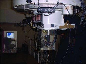
The SLODAR instrument can be compared with that of an SHWFS as used in AO to measure the aberrated optical wavefront. However, the SHWFS of the SLODAR instrument has a much wider FoV requiring the simultaneous measurement of double star optical wavefront gradients. The double stars observed by SLODAR can have angular separations up to several arcminutes. A functional diagram of the first ANU 7 × 7 SLODAR instrument installed on the ANU 24-inch telescope at SSO is shown in Figure 2. The optical diagram for the 17 × 17 SLODAR instrument on the ANU 40-inch telescope is similar to that shown in Figure 2 except for the 2 × 2 optic before the image intensifier. The 17 × 17 SLODAR instrument is shown in Figure 3.
The expanded optical block diagram of the 7 × 7 SLODAR instrument (first version) that attaches via bayonet mounted to the focus of the ANU 24-inch telescope at SSO. The diagram shows 5 × 5 SHWFS for simplification.

The ANU 17 × 17 SLODAR instrument (5.8-cm sub-apertures) on the ANU 40-inch telescope at SSO (photograph taken on 2006 June 18).
An advantage of the SLODAR instrument is a relatively simple optical design. A single collimator lens images the telescope pupil onto the microlens array (MLA) as shown in Figure 2. The collimating lens performs the following functions: (i) de-magnifies and collimates the incoming light beams of each double star component (i.e. point source at infinity); (ii) re-images the telescope pupil onto the MLA.
The MLA performs the function of optically dividing the telescope pupil into an array of sub-apertures. Each sub-aperture forms two spots (image of the double star) at their focal plane with image motion caused by aberrations in the double star optical wavefronts. The width of the sub-apertures, w, is comparable to the seeing coherent length, r 0, keeping the aberrated optical wavefront approximately linear. The sub-aperture spot displacement from mean position (centroid) is proportional to the averaged wavefront gradient (or slope). The images of the telescope pupils formed at the MLA are completely overlapped and are produced by double star components A and B. The individual lenslets (or sub-apertures) typically have slow focal ratios that image double star A and B components onto the image intensifier input (photocathode).
The image intensifier performs the function of applying a high gain (>1 000) to the incoming signal photons overcoming the high read noise of the high frame rate cameras used with the SLODAR instruments. The image intensifier allows fainter double stars to be observed, down to limiting magnitudes in the V band of approximately 5–6 (compared with 1–2 without the image intensifier). The image intensifier re-images and de-magnifies the MLA spot patterns onto the camera detector. Hence, the SLODAR instrument has two focal planes requiring correct adjustments during the calibration process.
The camera detectors used with the SLODAR instruments have the key features: (i) large format cameras (e.g. 1018 × 1008 pixel array) to image wide double stars; (ii) high frame rates (15, 20, 30, 200 fps) for layer wind speed measurements; (iii) short camera exposures of 2–8 ms in order to ‘freeze’ the turbulence. The camera exposures are on timescales equivalent to the turbulent-layer wind-crossing times of the sub-apertures.
Complementing the 17 × 17 instrument was the purpose-built real-time software (a graphical user interface (GUI) application), to satisfy the requirements for instrument control, processing and diagnostics, and autonomously logging of centroid data. The real-time software significantly increased the number of quality observed data sets.
4 DATA DESCRIPTION
4.1 Observational Plan
The scheduled observing runs for the SSO turbulence profiling are listed in Table 1. The observational plan was to sample the turbulence profile for each season over the course of the whole year. Turbulence profiling results were obtained from eight 1-week observational runs spanning years 2005 to 2006 with the 7 × 7 (runs 1–6) and 17 × 17 (runs 7 and 8) SLODAR instruments using the ANU 24-inch and 40-inch telescopes, respectively. Sampling over three consecutive months was conducted from 2005 November to 2006 January to examine any possible monthly variation in turbulence profiles. The first observational run in 2005 May provided a test run of the 7 × 7 SLODAR instrument on the ANU 24-inch telescope. A total of six observing runs were conducted with the ANU 7 × 7 SLODAR instrument, the final run being in 2006 January. The instrument changeover for the observational run in 2006 April to the 17 × 17 SLODAR instrument on the ANU 40-inch telescope was a response to the scientific requirement of needing more height sampling resolution bins and the measurement of the turbulent-layer wind speeds.
SLODAR Observational Runs at SSO
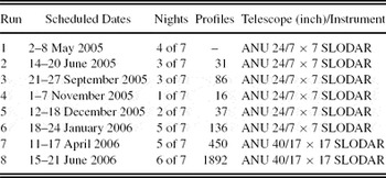
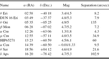
The observational list of double star targets is tabulated in Table 2. The limiting magnitude of the instruments, V ~ 5.5, limited the observational list to a couple (on occasions only one) of suitable targets for any given time at the telescope. The ability to alternate between ground-layer and free-atmosphere sampling is facilitated by switching between widely to narrowly separated double star targets. The increased number of profiles (data sets) for the final two observing runs was a result of changing from the manual process of logging data to automated logging with the introduction of the real-time software. The final run in 2006 June witnessed the full operation of the real-time software which captured 1 892 data sets for off-line processing.
Double Star Targets for SLODAR Observations at SSO
4.2 Data Acquisition
The SLODAR instrument delivers raw camera frames as shown in Figure 4 and are processed either by matlab (MathWorks 2005) (ANU 7 × 7 SLODAR instrument) or by the SLODAR real-time software (ANU 17 × 17 SLODAR instrument). The SLODAR real-time software has the capability to log raw camera frames but typically only the centroid data are logged.
An ensemble average over raw camera frames of (a) the SLODAR 7 × 7 instrument on the ANU 24-inch telescope at SSO and (b) the SLODAR 17 × 17 instrument on the ANU 40-inch telescope at SSO. The double stars observed are (a) αCrux and (b) αCen are aligned along the SHWFS x-direction.
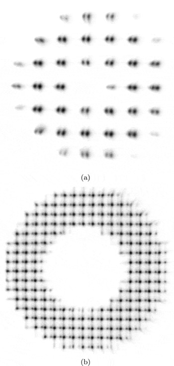
A summary of the observational data statistics is listed in Table 1. Data are acquired at 15 fps (Pulnix; JAI Inc. 2009, TM1020, 1 018 × 1 008 pixels) and 30 fps (Pixelink; PixeLINK 2009, A741, 1 280 × 1 024 pixels) to image larger separated double stars and 200 fps (Pulnix TM6740GE, 640 × 480 pixels) for high temporal sampling. A typical data set consists of a minimum of 600 camera frames (15 fps) or 4 000 camera frames (200 fps) for sufficient statistical sampling of the atmospheric turbulence.
5 DATA ANALYSIS
5.1 C 2 N (h) Profiles
In this section, we provide examples of consecutive C 2 N (h) turbulence profiles taken from the same double star target (or ‘group’ data sets having similar time stamps and height sampling) during the seventh observing run (2006 April 11–17) and the eighth observing run (2006 June 15–21). Note that we use the convention that h = 0 km defines the height of the telescope’s primary mirror. These observing runs had the highest number of data sets logged (see Table 1) and provide a useful visual indicator of the spatial–temporal evolution of the turbulence. Consecutive profiles for the seventh run are plotted in Figure 5. Example individual turbulence profiles from these group data sets are plotted in Figure 6.
SSO run 7. Examples of consecutive SLODAR turbulence profiles from difference spaced double star targets (height ranges). Each temporal plot represents a group of data sets from the same double star target (similar height sampling) measured during 2006 April 11–17. The vertical axis denotes height (km) and the horizontal axis denotes time (UTC). The colour denotes turbulence strength, C 2 N (h)dh (m 4−β). The plots are derived by interpolating the turbulence profiles onto a regular spaced grid at approximately Nyquist sampling. The blank regions represent times having no data. Note, h = 0 km defines the height of the telescope’s primary mirror.

SSO run 7. Examples of individual SLODAR turbulence profiles with each plot representing a single profile as represented in temporal plots of Figure 5 measured during 2006 April 11–17. The vertical axis denotes turbulence strength, C 2 N (h)dh (m 4−β), and the horizontal axis denotes height (km). Note, h = 0 km defines the height of the telescope’s primary mirror.

The temporal plots of the turbulence profiles show a number of dynamical characteristics: (i) intense turbulence occurring near the ground (below 100 m); (ii) turbulent layers that can fluctuate in intensity, appearing in ‘bursts’ with timescales of several minutes; this can have implications for different lines of sight; (iii) appearance to drift in altitude on some occasions rather than disperse before disappearing.
To quantify the structural distribution of the atmospheric turbulence, two statistical parameters are defined, namely hnnnn . The hnnnn parameter describes the fractional amount (0.0 to 1.0, with 1.0 being 100%) of turbulence below nnnn m as measured from the telescope’s primary mirror. The default value for nnnn is 500 m or h 500, but due to coarse height resolution sampling, the value of nnnn can be larger, e.g. 750 m or h 750. The hnnnn allows a qualitative assessment for the performance of ground-layer AO, which is favourable if the bulk of the turbulence is near the ground.
The third statistical parameter characterises the power-law slope index of the power spectrum of spatial phase fluctuations, βavg. The parameter βavg is representative of the entire atmospheric turbulence or averaged contribution of all layer heights. The βavg was determined by the best fit of the Δ = 0 theoretical covariance impulse response function for β ranging from 19/6 to 23/6 to the observed auto-covariance function, see Butterley et al. (Reference Butterley, Wilson and Sarazin2006). The implications of non-Kolmogorov turbulence (β ≠ 11/3) in the measurement of atmospheric turbulence and astronomical imaging are discussed by Stribling et al. (Reference Stribling, Welsh and Roggemann1995) and Goodwin (Reference Goodwin2009).
Fits of a non-Kolmogorov exponent to the SLODAR power spectrum (auto-covariance) are not provided in this paper. The fitted data have comparable error bars to Butterley et al. (Reference Butterley, Wilson and Sarazin2006) and that the best fit within the error bars typically produces exponent values that are non-Kolmogorov (less than 11/3). An exponent less than 11/3 causes the DIMM seeing to be overestimated due to increased image motion for small apertures (Goodwin Reference Goodwin2009). The power spectrum is relatively insensitive to the outer scale (Von Karman power spectrum) as noted by Butterley et al. (Reference Butterley, Wilson and Sarazin2006). A fit of the outer scale would typically need an outer scale smaller than the telescope (1 m), which is not typical of other measurements at other observatories (20–40 m). The outer-scale fit also has typically larger residuals for the larger offsets in the covariance function compared with the exponent fit.
The results measured during 2006 April 11–17 (run 7) and 2006 June 15–21 (run 8) using the ANU 17 × 17 SLODAR instrument on the ANU 40-inch telescope indicate an atmospheric turbulence structure that is dominated by strong ground-layer turbulence. This is evident in the summary h 500 parameter for all nights as shown in Figure 7. The summary h 500 parameter indicates that nearly 76% (run 7) and 91% (run 8) of the integrated turbulence is below 500 m. Note that in a few cases of limited height resolution sampling, h 500 will be more representative of higher altitudes, e.g. h 750, but this is a minority of the data sets.
Summary plot showing the fraction of turbulence below 500 m based on all observable nights measured during (a) SSO run 7: 2006 April 11–17 with the median fractional amount of turbulence below 500 m at 76% (based on 450 data sets); (b) SSO run 8: 2006 June 15–21 with the median fractional amount of turbulence below 500 m at 91% (based on 1 892 data sets).

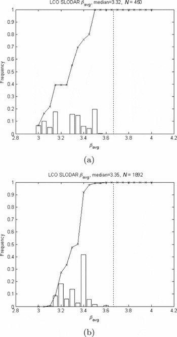
The summary βavg parameter for all nights is shown in Figure 8. The summary βavg parameter is found to have a median of 3.32 (run 7) and 3.35 (run 8) as compared with a Kolmogorov value of 3.67. This implies that the strong ground layer is non-Kolmogorov, causing a low βavg.
Summary plot showing the average power-law slope, βavg, of the spatial power spectrum of phase fluctuations based on all observable nights measured during (a) SSO run 7: 2006 April 11–17 with the median of 3.32 (based on 450 data sets) and (b) 2006 June 15–21 with the median of 3.35 (based on 1 892 data sets). For both cases, the values are noticeably less than the Kolmogorov value of 3.67 (dashed vertical line).
The summary seeing (for a wavelength of 0.5 μm) derived from the SLODAR function-fitting method (non-Kolmogorov analysis) and the DIMM method (Kolmogorov) is shown as a histogram in Figure 9. The median seeing values for the non-Kolmogorov and DIMM analysis (using SLODAR data) are 0.77 and 1.13 arcsec (run 7) and 1.1 and 1.33 arcsec (run 8). The discrepancy between the SLODAR (non-Kolmogorov) and DIMM (Kolmogorov) seeing calculation methods is most likely due to the low βavg values in the data (strong non-Kolmogorov effects). It is important to note that the seeing values have the mirror/dome seeing component removed (Goodwin et al. Reference Goodwin, Jenkins and Lambert2007), which is usually found to be a significant component. We note that the DIMM seeing of the SLODAR data, 1.13 and 1.33 arcsec, brackets the historical DIMM seeing measurements by Wood et al. (Reference Wood, Rodgers and Russell1995) of 1.25 arcsec.
Summary plot showing the seeing histograms of the SLODAR (non-Kolmogorov, red) method and DIMM (Kolmogorov, blue) method based on all observable nights measured during (a) SSO run 7: 2006 April 11–17 (based on 450 data sets) and (b) 2006 June 15–21 (based on 1 892 data sets). For both cases, the seeing values are reported at a wavelength of 0.5 μm.

5.2 V(h) Profiles
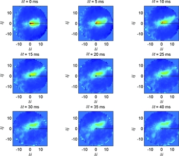
The translational velocity information of the turbulent layers can be retrieved by introducing gradual temporal offsets, δt, in the spatial cross-covariance function of wavefront gradients and by observing the corresponding displacement of peaks (Wilson Reference Wilson2002). The temporal offsets, δt, are integer multiples of the camera acquisition time (inverse of frame rate) and, therefore, must be sufficiently short to capture multiple observations of the turbulent layer as it moves across the telescope pupil. Typically, δt<100 ms, with camera acquisition times between 5 and 50 ms. A turbulent layer moving at velocity, v, will have its cross-covariance peak shifted by vδt from its location at δt = 0, aligned along the separation axis of the double star. By making several measurements of the spatial shifts in the cross-covariance peak for several sequential temporal offsets, δt, it is possible to trace the turbulent layer back to the origin to determine both height and velocity information. Examples of a layer wind speed measurement using the temporal spatial cross-covariance of centroid data during the seventh observing run (2006 April 11–17 ) are shown in Figure 10.
SSO run 7. Example temporal spatial cross-covariance of centroid data for layer wind speed determination as measured during 2006 April 11–17 with the CCD camera (TM6740GE) having a frame rate of 200 fps (area of interest read-out). The example is of the double star αCen with height resolution δh = 1.0 km. The double star separation axis (positive heights) is marked with a black line. The temporal offset, τ, is a multiple of the inverse of the frame rate, or 5 ms, starting from the top left panel with τ = 0 ms and the largest offset located at the bottom right panel with τ = 40 ms. The pixels represent the sub-aperture offsets (δi, δj) with physical size w = 5.8 cm. The wind speed of a layer can be estimated by s/τ, where s is the physical displacement of the covariance peak for a given temporal offset, τ. For this example, four separate layers are detected with speeds (1) 0.5 m/20 ms = 25 m s−1 (8 km); (2) 0.4 m/40 ms = 10 m s−1 (4 km); (3) 0.26 m/40 ms = 6.5 m s−1 (2 km); and (4) 0.18 m/40 ms = 4.5 m s−1 (0 km). Note, h = 0 km defines the height of the telescope’s primary mirror.
6 MODEL-OTP
A model-OTP is required to summarise the main characteristics of the measured atmospheric turbulence so that AO simulations can be performed and instrument performance can be predicted. The difficulty is that the atmospheric turbulence profiles follow a non-stationary process and therefore individual profiles are not representative for use in AO simulations. Of particular interest are the characteristics of the ground-layer and free-atmospheric turbulence, such as the contribution to the total turbulence integral (seeing), thickness and intensity of the ground layer, and if any persistent prominent layers exist.
To characterise the atmospheric turbulence, Model-OTPs have been synthesised from measurements obtained at other astronomical observatories. Tokovinin & Travouillon (Reference Tokovinin and Travouillon2006) note that previous model-OTPs that are based on the average or median profiles, such as in Abahamid et al. (Reference Abahamid, Jabiri, Vernin, Benkhaldoun, Azouit and Agabi2004), do not model the strong variability property of turbulence. Abahamid et al. (Reference Abahamid, Jabiri, Vernin, Benkhaldoun, Azouit and Agabi2004) point out that the turbulence intensity at any given altitude changes by several orders of magnitude and that real OTPs are typically dominated by a few strong layers. Hence, the use of only median or average techniques for OTPs to characterise the atmospheric turbulence for AO analysis may be misleading.
An example is the characterisation of the OTP above the Cerro Pachon (CP) astronomical site. The CP site was initially characterised during the 1998 Gemini site campaign (Vernin et al. Reference Vernin1998), in which seven discrete layers were modelled by Ellerbroek & Rigaut (Reference Ellerbroek and Rigaut2000), referred to as the ER2000 model. The ER2000 model has been used by other groups in AO simulations but is insufficient in two respects as noted by Tokovinin & Travouillon (Reference Tokovinin and Travouillon2006): (i) it does not address the variability of the real OTP and (ii) it was developed for the needs of classical and multi-conjugate AO that is mostly affected by high-altitude turbulence.
To resolve the limitations with the ER2000 model, and other similar models, Tokovinin & Travouillon (Reference Tokovinin and Travouillon2006) propose a new method to derive a more detailed statistical model-OTP suitable for GLAO analysis as well as other AO techniques. The proposed method has already been used by Andersen et al. (Reference Andersen2006) to model the OTP for Cerro Pachon for wide-field GLAO simulation for Gemini-South. An outline of the methodology for the model-OTP is given by Tokovinin & Travouillon (Reference Tokovinin and Travouillon2006). Note that the model-OTP derived in this paper also assumes a Kolmogorov turbulence model.
6.1 Methodology: Layer Strength Model
The model-OTP proposed by Tokovinin & Travouillon (Reference Tokovinin and Travouillon2006) separates the ground-layer (GL) statistics from the free-atmosphere (FA) statistics (observed to be independent). The GL zone is defined from the telescope (10–50 m) to some 500 m above the site. The FA zone is defined as all turbulence above the GL zone.
The Tokovinin & Travouillon (Reference Tokovinin and Travouillon2006) method is well suited to the SLODAR method. The SLODAR method has the ability to measure the GL and FA with sufficient height resolution by choosing appropriate double star separations. The GL can be measured with sufficient height resolution by selecting double stars having the widest separation.
The OTP is universally defined as the dependence of the refractive index structure constant C 2 N (measured in units m −2/3) at altitude h (measured in units of metres) above sea level (in this paper, h = 0 km is the height of the telescope’s primary mirror). The turbulence integral, J, is defined as
 \begin{equation}
J = \int {C_N^2 \left( h \right)} {\rm d}h
\end{equation}
\begin{equation}
J = \int {C_N^2 \left( h \right)} {\rm d}h
\end{equation}
(measured in units m 1/3) and is calculated over some altitude range.
The turbulence integral calculated over the entire height range covering the atmospheric turbulence (0–20 km), the total turbulence strength, can be expressed as the astronomical ‘seeing’ (in arcsec). The ‘seeing’ is the spot image FWHM of an unresolved object (e.g., unresolved star). The seeing for observations at a wavelength of λ = 500 nm at the zenith (Kolmogorov turbulence model) is given by
 \begin{equation}
\epsilon = [ {{J /{( {6.8 \times 10^{ - 13} } )}}} ]^{0.6}.
\end{equation}
\begin{equation}
\epsilon = [ {{J /{( {6.8 \times 10^{ - 13} } )}}} ]^{0.6}.
\end{equation}
The Tokovinin & Travouillon (Reference Tokovinin and Travouillon2006) method fits exponential equations to model the GL intensity and thickness. In this paper, we adopt a slightly different approach in that prominent layers are modelled as thin discrete layers, as representative of high-resolution turbulence profiles with micro-thermal balloon measurements. The thin layers preserve the relative strengths as well as the turbulence integrals J GL for the GL and J FA for the FA based on the ‘good’ (25%), ‘typical’ (50%), and ‘bad’ (75%) quartiles.
The J GL was calculated using the ‘seeing’ parameter (converted to J using Equation 8) and the h 500 parameter (fractional turbulence below 500 m), using the fact that J GL = h 500 J. The h 500 parameter can be calculated for all turbulence profiles as the maximum height is greater than 500 m and the height resolution of the zero height bin is less than 500 m for almost all observations. Hence, the h 500 parameter is suitable for the calculation of J GL. The J FA was calculated using the fact that J FA = J − J GL. For the simplicity of calculations, it was assumed that the GL and FA are both modelled by a Kolmogorov turbulence model. With three turbulence profiles based on thin layers for each of the GL and FA, it is possible to construct an OTP model having nine possible outcomes with respective probabilities.
The models sufficiently cover half of the conditions (25%–75%) expected at the astronomical site within which a probability of 25% is assigned to ‘good’, 50% is assigned to ‘typical’, and 25% is assigned to ‘bad’ for GL and FA turbulence profiles. The total turbulence profile is a combination of the GL and FA turbulence profiles with probability equal to the respective GL and FA probabilities being multiplied. The assignment of probabilities to all possible turbulence profile outcomes of the model allows a relative importance to be assigned. The model does not sufficiently represent the extreme cases of very ‘good’ (0%–25%) and very ‘bad’ (75%–100%) conditions. It is noted that the very ‘bad’ condition is of most concern as AO may not provide sufficient wavefront correction for scientific operations. Sufficient representation for the very ‘good’ and very ‘bad’ conditions can be obtained by extrapolation, scaling the layer relative fractional amounts by the J GL and J FA turbulence integrals, using values from the respective cumulative density function (CDF) plots.
6.1.1 Ground-Layer Model-OTP
To derive the GL model-OTP, we consider three model turbulence profiles derived from averaging a group of observational profiles in intervals centred on the CDF quartiles for the J GL turbulence integral. The ‘good’ model turbulence profile is derived from averaging profiles having maximum sampling height, H max, greater than 500 m but less than 2 000 m (ground-layer sampling) within the 15%–35% interval of the cumulative values of J GL. Likewise, the same holds for the ‘typical’ model turbulence profile, within the 40%–60% interval, and the ‘bad’ model turbulence profile, within the 65%–85% interval. The relatively small value of N OTP for the GL analysis reflects the fact that only a limited number of data sets suitable for GL sampling at SSO were observed. The values relating to the GL model turbulence profiles are listed in Table 3.
Levels of the Cumulative Distributions of J GL Used in the Calculation of a Representative Ground-Layer Profile, ‘Good’, ‘Typical’, and ‘Bad’ for SSO (Runs 1–8: 2005 May to 2006 June)
From Table 3 we see that some intervals have more turbulence profiles, due to the J GL distribution consisting of a mixture of both GL and FA turbulence profiles, with a portion not meeting the maximum sampling height criterion. The average maximum height range, H max , is 0.72–1.07 km and the average height resolution, δh , is 72–108 m.
Figure 11 shows the GL model turbulence profiles obtained from averaging GL profiles within certain interval ranges of the J GL distribution to represent ‘good’, ‘typical’, and ‘bad’ seeing conditions, as summarised in Table 3.
Continuous GL model-OTP for SSO (Runs 1–8: 2005 May to 2006 June): squares ‘good’, diamonds ‘typical’, and circles ‘bad’ (a) averaged profiles, error bars are the 95% confidence interval, and (b) corresponding CDF profiles.
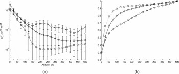
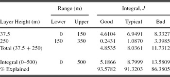
A thin-layer GL model-OTP is required to be derived from the continuous GL model-OTP. A thin-layer GL model-OTP is an accurate representation of high-resolution OTPs (Azouit & Vernin Reference Azouit and Vernin2005), as well as compatible for AO simulations (using phase screens to represent thin layers). For the thin-layer GL model-OTP, we define two layers at heights 37.5 and 250 m to best represent the continuous GL model-OTP (Figure 11). To calculate the strengths of the layers, an integral (lower, upper) centred on the layer heights of the continuous GL model-OTP is performed. To compare how well layer integrals explain the model, the total layer integral (37.5 m + 250 m) is compared with the total GL integral from 0 to 500 m (calculated from the continuous GL model-OTP). The results are listed in Table 4.
Turbulence Integrals for the Thin-Layer Model-OTP for the Ground Layer, J in Units of 10−13 m 1/3 for SSO (Runs 1–8: 2005 May to 2006 June)
The fractional strengths can be multiplied by J GL according to cumulative level values obtained from its corresponding CDF plot. The model is based on the cumulative levels 25%, 50%, and 75%, but other levels can be used for extreme conditions, e.g. 10%, 50%, and 90%, providing some flexibility for a custom model-OTP.
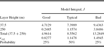
The turbulence integral strengths of the model thin layers are calculated by multiplying the fractional amounts with the cumulative levels 25%, 50%, and 75% of J GL. The final model thin layers and their turbulence integral, with total ground-layer seeing, εGL, and model probability, are listed in Table 5.
Final Turbulence Integrals for the GL Thin-Layer Model-OTP, J in Units of 10−13 m 1/3 for SSO (Runs 1–8: 2005 May to 2006 June)
6.1.2 Free-Atmosphere Model-OTP
To derive the FA model, we follow a similar approach to that described for the GL model. This involves deriving three model turbulence profiles from averaging a group of observational profiles within representative intervals of CDF values for the J FA turbulence integral. The ‘good’ model turbulence profile is derived from averaging profiles having maximum sampling height, H max, greater than 16 000 m but less than 20 000 m (free-atmosphere sampling) within the 15%–35% interval of the cumulative values of J FA. Likewise, the same holds for the ‘typical’ model turbulence profile, within the 40%–60% interval, and the ‘bad’ model turbulence profile, within the 65%–85% interval. The values relating to the FA model turbulence profiles are listed in Table 6.
Levels of the Cumulative Distributions of J FA Used in the Calculation of a Representative Ground-Layer Profile, ‘Good’, ‘Typical’, and ‘Bad’ for SSO (Runs 1–8: 2005 May to 2006 June)
From Table 6 we see that some intervals have more turbulence profiles, due to the J FA distribution consisting of a mixture of both GL and FA turbulence profiles, with a portion not meeting the maximum sampling height criteria. The average maximum height range, H max , is 17.0–17.3 km and the average height resolution, δh , is 1 095–1 338 m.
Figure 12 shows the FA model turbulence profiles obtained from averaging FA profiles within certain interval ranges of the J FA distribution to represent ‘good’, ‘typical’, and ‘bad’ seeing conditions, as summarised in Table 6.
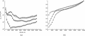
Continuous FA model-OTP for SSO (Runs 1–8: 2005 May to 2006 June): squares ‘good’, diamonds ‘typical’, and circles ‘bad’ (a) averaged profiles, error bars are the 95% confidence interval, and (b) corresponding CDF profiles.
A thin-layer FA model-OTP is required to be derived from the continuous FA model-OTP. A thin-layer FA model-OTP is an accurate representation of high-resolution OTPs (Azouit & Vernin Reference Azouit and Vernin2005) as well as compatible for adaptive optic simulations (using phase screens to represent thin layers). For the thin-layer FA model-OTP, we define five layers at heights 1 000, 3 000, 6 000, 9 000, and 13 500 m to best represent the continuous FA model-OTP (Figure 12). To calculate the strengths of the layers, an integral (lower, upper) centred on the layer heights of the continuous FA model-OTP is performed. To compare how well layer integrals explain the model, the total layer integral (1 000 + 3 000 + 6 000 + 9 000 + 13 500 m) is compared with the total FA integral from 500 to 16 000 m (calculated from the continuous FA model-OTP). The results are listed in Table 7.
Turbulence Integrals for the Thin-Layer Model-OTP for the Free Atmosphere, J in Units of 10−13 m 1/3 for SSO (Runs 1–8: 2005 May to 2006 June)
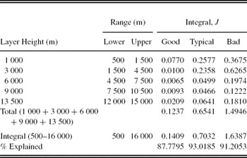
The FA model-OTP in Table 7 has a gap in binning between 10.5 and 12 km as well above 15 km. This is because we rarely saw any evidence for turbulence at those heights in the continuous FA profile of Figure 12. There was also an attempt to keep the number of model layers to minimum as well as keeping equal bin widths of 3000 m. The gap in binning will result in a slight bias to increase the relative strength of the FA lower layers, causing the isoplanatic angle to be slightly larger (providing an optimistic estimate). The value of the bias is expected to be small.
The fractional strengths can be multiplied by J FA according to cumulative levels obtained from its CDF plot. The model is based on the cumulative levels 25%, 50%, and 75%, but for other levels extreme conditions can be used, e.g. 10%, 50%, and 90%, providing some flexibility for a custom model-OTP.
The turbulence integral strengths of the model thin layers are calculated by multiplying the fractional amounts with the cumulative levels 25%, 50%, and 75% of J FA. The final model thin layers and their turbulence integral, with the total free-atmosphere seeing, εFA, and model probability, are listed in Table 8.
Final Turbulence Integrals for the FA Thin-Layer Model-OTP, J in Units of 10−13 m 1/3 for SSO (Runs 1–8: 2005 May to 2006 June)
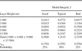
The total integrated turbulence of the thin-layer FA model as shown in Table 8 is approximately twice that of the total integrated turbulence of the binned layer continuous FA model as shown in Table 7. A likely explanation for the scale factor of ~2 may be the result that the parameter J FA has been overestimated (turbulence integral in the free atmosphere computed based on total seeing and H 500) compared with the direct turbulence integrals of the averaged measured profiles. The total strength of the weaker free-atmosphere layers (not location) as measured by SLODAR is somewhat underestimated (low S/N). The factor of a ~2 scaling increase makes the free-atmosphere seeing in the final model a conservative estimate.
6.2 Methodology: Layer Wind Speed and Direction Model
To model the turbulent layer speeds, a Bufton wind speed profile model is used (see Equation 9). To model the ‘good’, ‘typical’, and ‘bad’ conditions, three separate Bufton wind profiles are presented based on data found in the literature (Avila et al. Reference Avila2003; Tokovinin, Baumont, & Vasquez Reference Tokovinin, Baumont and Vasquez2003; Azouit & Vernin Reference Azouit and Vernin2005). The wind profiles are not based on fits to our data as it is not always possible to obtain a sufficient sample of layer wind speeds with our SLODAR data due to (i) low camera frame rates, (ii) finite camera exposures, (iii) weakness of a layer, and (iv) short boiling lifetimes (layer de-correlates rapidly). The Bufton wind profile model is given by
 \begin{equation}
v(h) = v_G+v_{\rm T} {\rm exp} \left[-\left(\frac{h-H_{\rm T}}{L_{\rm T}}\right)^2\right],
\end{equation}
\begin{equation}
v(h) = v_G+v_{\rm T} {\rm exp} \left[-\left(\frac{h-H_{\rm T}}{L_{\rm T}}\right)^2\right],
\end{equation}
where vG denotes the wind velocity at low altitude, v T denotes the wind velocity at the tropopause, H T denotes the height of tropopause, L T denotes the thickness of the tropopause layer.
The parameters of the Bufton wind model for the ‘good’, ‘typical’, and ‘bad’ conditions used in the analysis are listed in Table 9. The wind model associates strong ground-layer wind speeds with stronger free-atmosphere wind speeds that have a broader upper atmosphere extent (Azouit & Vernin Reference Azouit and Vernin2005; Tokovinin et al. Reference Tokovinin, Baumont and Vasquez2003; Avila et al. Reference Avila2003). To simplify the model, the ‘good’, ‘typical’, and ‘bad’ conditions are represented by the same profile and referenced to the ground-layer wind direction, set to 0°. The free-atmosphere layers can travel in a direction perpendicular to the ground-layer direction. The wind direction model, ψ(h), for the ‘good’, ‘typical’, and ‘bad’ conditions is defined as
 \begin{equation}
\psi (h) = a(1-{\rm exp}(-h/b))
\end{equation}
\begin{equation}
\psi (h) = a(1-{\rm exp}(-h/b))
\end{equation}
where a = 101.93 and b = 3 255.4 are used.
Bufton Wind Model
6.2.1 Turbulent-Layer Wind Model
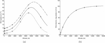
To model the turbulent-layer wind speed and direction for the SSO (runs 1–8: 2005 May to 2006 June) runs, a Bufton wind speed model together with layer height information from the model-OTP is used. The model-OTP layer heights for the ground layer and free atmosphere are used in the Bufton equation to obtain the model layer wind speed values. The model relative layer wind directions are obtained by using the model-OTP layer heights in the wind direction, φ(h), defined in Equation (10). The wind speed model and wind direction model values for the SSO (runs 1–8: 2005 May to 2006 June) model-OTP are shown in Figure 13 and tabulated in Table 10.
Tabulated Values for the Model Wind Speed and Model Wind Direction for the GL and FA Model-OTP Layers for the SSO (Runs 1–8: 2005 May to 2006 June) Model
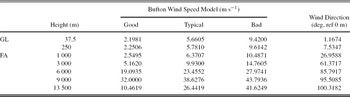
Wind model-OTP for the SSO (Runs 1–8: 2005 May to 2006 June) runs: squares ‘good’, diamonds ‘typical’, and circles ‘bad’ (a) Bufton wind profile and (b) wind direction (empirical). Layer heights for model-OTP for the SSO (Runs 1–8: 2005 May to 2006 June) model are marked as symbols.
6.3 Summary Model-OTP
The summary model-OTP (Kolmogorov) is the combination of the ‘good’, ‘typical’, and ‘bad’ GL and FA model-OTPs resulting in a set of nine possible thin-layer turbulence profiles. Each turbulence profile of the model-OTP includes information about the turbulence layer strength, wind speed, and wind direction.
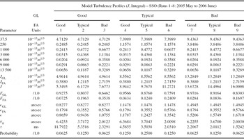
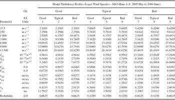
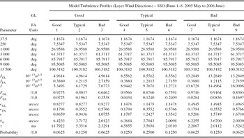
A detailed summary table of the summary model-OTPs describing the observations at Siding Spring Observatory, Australia, for the SSO (runs 1–8: 2005 May to 2006 June) runs is presented in Table 11 (turbulence integrals), Table 12 (turbulence layer wind speeds), and Table 13 (turbulence layer wind direction). Note that the model-OTP seeing, ε, for the typical GL + FA of 1.24 arcsec is similar to the historical median DIMM seeing of 1.25 arcsec reported by Wood et al. (Reference Wood, Rodgers and Russell1995).
Tabulated Values for the Final Model-OTP for SSO (Runs 1–8: 2005 May to 2006 June), with Layers Specified as Turbulence Integral, J, in Units 10−13 m 1/3
Tabulated Values for the Final Model-OTP for the SSO (Runs 1–8: 2005 May to 2006 June), with Layers Specified as Wind Speeds
Tabulated Values for the Final Model-OTP for the SSO (Runs 1–8: 2005 May to 2006 June), with Layers Specified as Wind Directions
7 CONCLUSIONS
This paper has reported on our turbulence profiling observational results performed at SSO. A summary of results with example data has been presented for measurement spanning years 2005 to 2006 using the 7 × 7 (runs 1–6) and 17 × 17 (runs 7 and 8) SLODAR instruments. The observational results have facilitated the site characterisation of the optical turbulence profile with the implementation of the model-OTP (Kolmogorov) for SSO. The model-OTP describes the turbulence layer strength (Table 11), layer wind speed (Table 12), and layer wind direction (Table 13). The model-OTP is useful for the prediction of AO performance at SSO (forthcoming paper) using simulation codes. Prior to the commencement of our SLODAR campaign, the seeing statistics were relatively well understood with DIMM seeing measurements (Wood et al. Reference Wood, Rodgers and Russell1995), whereas the vertical structure of the turbulence profile structure was relatively unknown, with only a few SCIDAR profiles reported by Klueckers et al. (Reference Klueckers, Wooder, Nicholls, Adcock, Munro and Dainty1998). The following conclusions can be stated about the atmospheric turbulence above SSO based on our data:
-
• A measured median atmospheric seeing of around 1.2 arcsec (Kolmogorov model with mirror/dome seeing removed). The seeing is discussed in Section 5.1.
-
• Ground-layer turbulence dominates, with ~80% turbulence below 500 m (h 500). The structure of the turbulence is discussed in Section 5.1. The presence of a strong ground layer was also discovered during site measurements at Mount John University Observatory (Mohr, Johnston, & Cottrell Reference Mohr, Johnston and Cottrell2010). The dominant ground layer has promising implications for GLAO. A forthcoming paper will investigate the performance of GLAO based on the model-OTP for SSO.
-
• Non-Kolmogorov turbulence is observed especially for ground layer, with βavg ~ 10/3. The power-law slope of the spatial phase fluctuations is discussed in Section 5.1. The non-Kolmogorov spectrum results in a different scaling of seeing with wavelength to that conventionally assumed.
-
• Turbulence profiles show a number of dynamical characteristics: (i) are most intense near the ground (below 100 m) and (ii) fluctuate in intensity, appearing in ‘bursts’ with timescales of several minutes. These characteristics are shown in Figure 6 as a sequence of turbulence profiles.
-
• Mirror/dome seeing can be a significant fraction of the ground-layer turbulence. This is evident as a zero-height static contribution in the turbulent-layer wind speed measurements (refer to Section 5.2 and Figure 10).
-
• The free-atmosphere turbulence is comparable to ‘good’ seeing sites. From the model-OTP shown in Table 11, the free-atmosphere seeing for SSO is 0.18 (25%), 0.36 (50%), and 0.58 (75%) arcsec. The Cerro Pachon (seeing ~0.75) model (Tokovinin & Travouillon Reference Travouillon2006) for the free-atmosphere reports 0.29 (25%), 0.40 (50%), and 0.55 (75%) arcsec.
ACKNOWLEDGMENTS
This work makes use of observational data and analysis provided by MG’s PhD thesis research (submitted 2009) conducted at the Research School of Astronomy and Astrophysics (RSAA) of the Australian National University (ANU). We thank Peter Conroy (ANU) for the design and manufacture of the instrumentation. The authors are grateful to Jon Lawrence of the Australian Astronomical Observatory (AAO) for his suggestions on the original version of the manuscript and to the referees for their comments.


