


1 Introduction
The compactly supported
 $\mathbb {A}^1$
-Euler characteristic
$\mathbb {A}^1$
-Euler characteristic
 $\chi _c^{\mathrm {mot}}$
was first introduced in work of Hoyois [Reference HoyoisHoy14], later refined by Levine [Reference LevineLev20] for smooth projective schemes and extended to general varieties over a field in characteristic zero by Arcila-Maya, Bethea, Opie, Wickelgren and Zakharevich [Reference Arcila-Maya, Bethea, Opie, Wickelgren and ZakharevichAMBO+22] and Röndigs [Reference RöndigsRön25], and to general varieties in characteristic not
$\chi _c^{\mathrm {mot}}$
was first introduced in work of Hoyois [Reference HoyoisHoy14], later refined by Levine [Reference LevineLev20] for smooth projective schemes and extended to general varieties over a field in characteristic zero by Arcila-Maya, Bethea, Opie, Wickelgren and Zakharevich [Reference Arcila-Maya, Bethea, Opie, Wickelgren and ZakharevichAMBO+22] and Röndigs [Reference RöndigsRön25], and to general varieties in characteristic not
 $2$
by Levine, Pepin-Lehalleur and Srinivas in [Reference Levine, Lehalleur and SrinivasLPS24]. It is an algebro-geometric invariant that refines both the real and complex Euler characteristic of topological manifolds, as well as some additional arithmetic data. As opposed to the classical Euler characteristic, which takes values in
$2$
by Levine, Pepin-Lehalleur and Srinivas in [Reference Levine, Lehalleur and SrinivasLPS24]. It is an algebro-geometric invariant that refines both the real and complex Euler characteristic of topological manifolds, as well as some additional arithmetic data. As opposed to the classical Euler characteristic, which takes values in
 $\mathbb {Z}$
, the compactly supported
$\mathbb {Z}$
, the compactly supported
 $\mathbb {A}^1$
-Euler characteristic takes values in the Grothendieck-Witt ring
$\mathbb {A}^1$
-Euler characteristic takes values in the Grothendieck-Witt ring
 $\operatorname {\mathrm {GW}}(k)$
of the base field k, so it contains “quadratic” information. However, unlike the classical Euler characteristic, it can be difficult to compute
$\operatorname {\mathrm {GW}}(k)$
of the base field k, so it contains “quadratic” information. However, unlike the classical Euler characteristic, it can be difficult to compute
 $\chi _c^{\mathrm {mot}}(X)$
even when X is a smooth projective variety. Papers such as [Reference Levine, Lehalleur and SrinivasLPS24] and [Reference ViergeverVie25] use the motivic Gauß-Bonnet Theorem of Levine-Raksit [Reference Levine and RaksitLR20] to compute the compactly supported
$\chi _c^{\mathrm {mot}}(X)$
even when X is a smooth projective variety. Papers such as [Reference Levine, Lehalleur and SrinivasLPS24] and [Reference ViergeverVie25] use the motivic Gauß-Bonnet Theorem of Levine-Raksit [Reference Levine and RaksitLR20] to compute the compactly supported
 $\mathbb {A}^1$
-Euler characteristic of hypersurfaces in
$\mathbb {A}^1$
-Euler characteristic of hypersurfaces in
 $\mathbb {P}^n$
and complete intersections of hypersurfaces of the same degree in
$\mathbb {P}^n$
and complete intersections of hypersurfaces of the same degree in
 $\mathbb {P}^n$
, and Brazelton, McKean and Pauli computed the compactly supported
$\mathbb {P}^n$
, and Brazelton, McKean and Pauli computed the compactly supported
 $\mathbb {A}^1$
-Euler characteristics of Grassmannians in [Reference Brazelton, McKean and PauliBMP23], using
$\mathbb {A}^1$
-Euler characteristics of Grassmannians in [Reference Brazelton, McKean and PauliBMP23], using
 $\mathbb {A}^1$
-degrees. While this invariant can be difficult to work with, it has found use in enumerative geometry since it is analogous to the classical Euler characteristic of a manifold. We may use this invariant to obtain enumerative geometry counts which take values in
$\mathbb {A}^1$
-degrees. While this invariant can be difficult to work with, it has found use in enumerative geometry since it is analogous to the classical Euler characteristic of a manifold. We may use this invariant to obtain enumerative geometry counts which take values in
 $\operatorname {\mathrm {GW}}(k)$
and papers such as [Reference Pajwani and PálPPa] by the first author and Pál, and [Reference Blomme, Brugallé and GarayBBGar] by Blomme, Brugallé and Garay, use the compactly supported
$\operatorname {\mathrm {GW}}(k)$
and papers such as [Reference Pajwani and PálPPa] by the first author and Pál, and [Reference Blomme, Brugallé and GarayBBGar] by Blomme, Brugallé and Garay, use the compactly supported
 $\mathbb {A}^1$
-Euler characteristic to obtain arithmetic refinements of results in complex enumerative geometry, the first over a general base field and the second over the real numbers.
$\mathbb {A}^1$
-Euler characteristic to obtain arithmetic refinements of results in complex enumerative geometry, the first over a general base field and the second over the real numbers.
This paper is concerned with the compactly supported
 $\mathbb {A}^1$
-Euler characteristic of symmetric powers of varieties, which can be viewed as moduli spaces of effective zero-cycles. These geometric objects are closely related to Hilbert schemes of points via the birational Hilbert-Chow morphism. They are of particular interest to people studying enumerative geometry, appearing for example in the Göttsche formula for Euler characteristics of Hilbert schemes of surfaces ([Reference GöttscheGöt90, Theorem 0.1], [Reference Pajwani and PálPPa, Corollary 8.18]). Since symmetric powers of a variety X are almost always singular if
$\mathbb {A}^1$
-Euler characteristic of symmetric powers of varieties, which can be viewed as moduli spaces of effective zero-cycles. These geometric objects are closely related to Hilbert schemes of points via the birational Hilbert-Chow morphism. They are of particular interest to people studying enumerative geometry, appearing for example in the Göttsche formula for Euler characteristics of Hilbert schemes of surfaces ([Reference GöttscheGöt90, Theorem 0.1], [Reference Pajwani and PálPPa, Corollary 8.18]). Since symmetric powers of a variety X are almost always singular if
 $\mathrm {dim}(X)\geq 2$
, we cannot directly apply the motivic Gauß–Bonnet theorem of [Reference Levine and RaksitLR20] to them, and as such their compactly supported
$\mathrm {dim}(X)\geq 2$
, we cannot directly apply the motivic Gauß–Bonnet theorem of [Reference Levine and RaksitLR20] to them, and as such their compactly supported
 $\mathbb {A}^1$
-Euler characteristics seem difficult to compute directly. However, symmetric powers of a variety furnish an additional structure on
$\mathbb {A}^1$
-Euler characteristics seem difficult to compute directly. However, symmetric powers of a variety furnish an additional structure on
 $\mathrm {K}_0(\mathrm {Var}_k)$
, known as a power structure (see Definition 2.4). Therefore, we instead use the results of [Reference Pajwani and PálPP25] to utilise power structures defined on
$\mathrm {K}_0(\mathrm {Var}_k)$
, known as a power structure (see Definition 2.4). Therefore, we instead use the results of [Reference Pajwani and PálPP25] to utilise power structures defined on
 $\mathrm {GW}(k)$
in order to compute the motivic Euler characteristics of symmetric powers. We give a formula for the compactly supported
$\mathrm {GW}(k)$
in order to compute the motivic Euler characteristics of symmetric powers. We give a formula for the compactly supported
 $\mathbb {A}^1$
-Euler characteristic of symmetric powers of a class of varieties that we call
$\mathbb {A}^1$
-Euler characteristic of symmetric powers of a class of varieties that we call
 $\mathrm {K}_0$
-étale linear. Informally,
$\mathrm {K}_0$
-étale linear. Informally,
 $\mathrm {K}_0$
-étale linear varieties are varieties whose class in
$\mathrm {K}_0$
-étale linear varieties are varieties whose class in
 $\mathrm {K}_0(\mathrm {Var}_{k})$
decomposes into a sum with terms
$\mathrm {K}_0(\mathrm {Var}_{k})$
decomposes into a sum with terms
 $[\mathbb {A}^n_L]$
, where
$[\mathbb {A}^n_L]$
, where
 $L/k$
is a finite separable extension (see Definition 3.1). These form a class of varieties containing many widely studied varieties, such as cellular varieties (Lemma 3.3), del Pezzo surfaces of degree
$L/k$
is a finite separable extension (see Definition 3.1). These form a class of varieties containing many widely studied varieties, such as cellular varieties (Lemma 3.3), del Pezzo surfaces of degree
 $\geq 5$
(Theorem 5.6), certain tori (Example 3.1) and others. Our main result can be stated as follows:
$\geq 5$
(Theorem 5.6), certain tori (Example 3.1) and others. Our main result can be stated as follows:
Theorem 1.1 (Theorem 4.8)
Let X be a
 $\mathrm {K}_0$
-étale linear variety over field k of characteristic
$\mathrm {K}_0$
-étale linear variety over field k of characteristic
 $\neq 2$
(see Definition 3.1), and for
$\neq 2$
(see Definition 3.1), and for
 $n\in \mathbb {Z}_{\geq 0}$
, write
$n\in \mathbb {Z}_{\geq 0}$
, write
 $X^{(n)} := \mathrm {Sym}^n(X)$
. Then
$X^{(n)} := \mathrm {Sym}^n(X)$
. Then
 $\chi _c^{\mathrm {mot}}(X^{(n)}) = a_n(\chi _c^{\mathrm {mot}}(X))$
for every n, where
$\chi _c^{\mathrm {mot}}(X^{(n)}) = a_n(\chi _c^{\mathrm {mot}}(X))$
for every n, where
 $a_n$
denotes the function defining the power structure on
$a_n$
denotes the function defining the power structure on
 $\operatorname {\mathrm {GW}}(k)$
as in Definition 2.5.
$\operatorname {\mathrm {GW}}(k)$
as in Definition 2.5.
The power of the above theorem lies in the fact that it is much easier to work with the power structure on
 $\operatorname {\mathrm {GW}}(k)$
than it is to decompose the symmetric powers of
$\operatorname {\mathrm {GW}}(k)$
than it is to decompose the symmetric powers of
 $\mathrm {K}_0$
-étale linear varieties in general.
$\mathrm {K}_0$
-étale linear varieties in general.
We say a variety X is symmetrisable if
 $\chi _c^{\mathrm {mot}}$
respects the power structure as in our main result, i.e., if
$\chi _c^{\mathrm {mot}}$
respects the power structure as in our main result, i.e., if
 $\chi _c^{\mathrm {mot}}(X^{(n)}) = a_n(\chi _c^{\mathrm {mot}}(X))$
for all n, see Definition 4.1. Corollary 6.5 and Lemma 6.6 show that the class of symmetrisable varieties contains curves of genus
$\chi _c^{\mathrm {mot}}(X^{(n)}) = a_n(\chi _c^{\mathrm {mot}}(X))$
for all n, see Definition 4.1. Corollary 6.5 and Lemma 6.6 show that the class of symmetrisable varieties contains curves of genus
 $1$
and that these are not
$1$
and that these are not
 $\mathrm {K}_0$
-étale linear.
$\mathrm {K}_0$
-étale linear.
Theorem 1.2 (Corollary 6.5 and Lemma 6.6)
Let C be a curve of genus
 $1$
, and let k be a field of characteristic
$1$
, and let k be a field of characteristic
 $0$
. Then C is symmetrisable, but it is not
$0$
. Then C is symmetrisable, but it is not
 $\mathrm {K}_0$
-étale linear.
$\mathrm {K}_0$
-étale linear.
Additionally, we show in Theorem 4.14 that a variety over k must itself be symmetrisable if it becomes symmetrisable after base change to a finite extension
 $L/k$
of odd degree. We use this to show that even dimensional Severi–Brauer varieties are symmetrisable in Corollary 4.16 even though they may not be
$L/k$
of odd degree. We use this to show that even dimensional Severi–Brauer varieties are symmetrisable in Corollary 4.16 even though they may not be
 $\mathrm {K}_0$
-étale linear. While we only show that curves of genus
$\mathrm {K}_0$
-étale linear. While we only show that curves of genus
 $\leq 1$
are symmetrisable, in [Reference Bröring and ViergeverBV25, Proposition 26], Bröring and the third author show that all curves are symmetrisable using different techniques. Moreover, in [Reference BröringBrö26, Theorem 8.3, Theorem 8.6], it is shown that for any smooth projective variety,
$\leq 1$
are symmetrisable, in [Reference Bröring and ViergeverBV25, Proposition 26], Bröring and the third author show that all curves are symmetrisable using different techniques. Moreover, in [Reference BröringBrö26, Theorem 8.3, Theorem 8.6], it is shown that for any smooth projective variety,
 $\chi _c^{\mathrm {mot}}(X^{(n)})=a_n(\chi _c^{\mathrm {mot}}(X))$
whenever
$\chi _c^{\mathrm {mot}}(X^{(n)})=a_n(\chi _c^{\mathrm {mot}}(X))$
whenever
 $n \leq 3$
, and the smooth projective assumption can be removed in characteristic
$n \leq 3$
, and the smooth projective assumption can be removed in characteristic
 $0$
(see [Reference BröringBrö26, Theorem 8.9]).
$0$
(see [Reference BröringBrö26, Theorem 8.9]).
We apply our main result in Theorem 5.8 to compute
 $\chi _c^{\mathrm {mot}}(X^{(3)})$
for X a specific cubic surface; a computation which we believe would be difficult to do without using the power structure. Similarly, we use it to compute a generating series for
$\chi _c^{\mathrm {mot}}(X^{(3)})$
for X a specific cubic surface; a computation which we believe would be difficult to do without using the power structure. Similarly, we use it to compute a generating series for
 $\chi _c^{\mathrm {mot}}$
of the symmetric powers of a Grassmannian.
$\chi _c^{\mathrm {mot}}$
of the symmetric powers of a Grassmannian.
Theorem 1.3 (Corollary 5.3)
There is a generating series for the compactly supported
 $\mathbb {A}^1$
-Euler characteristic of the symmetric power of a Grassmannian:
$\mathbb {A}^1$
-Euler characteristic of the symmetric power of a Grassmannian:
 $$ \begin{align*}\sum_{n=0}^\infty \chi_c^{\mathrm{mot}}(\mathrm{Gr}(d,r)^{(n)})t^n = (1-t)^{-e(d,r)} (1- (\langle -1 \rangle t))^{-o(d,r)} \in \operatorname{\mathrm{GW}}(k)[[t]], \end{align*} $$
where
 $e(d,r)$
is the d-th entry in the r-th row of Losanitsch’s triangle, and
$e(d,r)$
is the d-th entry in the r-th row of Losanitsch’s triangle, and
 $o(d,r)$
is given by
$o(d,r)$
is given by
 $\binom {r}{d} - e(d,r)$
.
$\binom {r}{d} - e(d,r)$
.
The above result enriches the generating series of the classical Euler characteristic of symmetric powers of complex Grassmannians, as the rank map
 $\operatorname {\mathrm {GW}}(k) \rightarrow \mathbb {Z}$
sends the form
$\operatorname {\mathrm {GW}}(k) \rightarrow \mathbb {Z}$
sends the form
 $\langle -1 \rangle $
to
$\langle -1 \rangle $
to
 $1$
and the sum
$1$
and the sum
 $e(d,r) + o(d,r)$
is the binomial coefficient
$e(d,r) + o(d,r)$
is the binomial coefficient
 $\binom {r}{d}$
. Applying the sign map
$\binom {r}{d}$
. Applying the sign map
 $\langle -1 \rangle \mapsto -1$
to the formula of Theorem 5.1 yields
$\langle -1 \rangle \mapsto -1$
to the formula of Theorem 5.1 yields
 $0$
if r is even and d is odd and
$0$
if r is even and d is odd and
 $\binom {\lfloor r/2 \rfloor }{\lfloor d/2 \rfloor }$
otherwise, which is precisely the classical Euler characteristic of the real Grassmannian
$\binom {\lfloor r/2 \rfloor }{\lfloor d/2 \rfloor }$
otherwise, which is precisely the classical Euler characteristic of the real Grassmannian
 $\operatorname {\mathrm {Gr}}(d,r)/\mathbb {R}$
, in concordance with [Reference LevineLev20, Remark 2.3.1].
$\operatorname {\mathrm {Gr}}(d,r)/\mathbb {R}$
, in concordance with [Reference LevineLev20, Remark 2.3.1].
In Section 2, we recall notions required for our paper. We first restate the definition of the compactly supported
 $\mathbb {A}^1$
-Euler characteristic in Definition 2.3. To compute the compactly supported
$\mathbb {A}^1$
-Euler characteristic in Definition 2.3. To compute the compactly supported
 $\mathbb {A}^1$
-Euler characteristics of symmetric powers of varieties, we use the notion of a power structure on a ring, see Definition 2.4. We recall the existence of natural power structures on both
$\mathbb {A}^1$
-Euler characteristics of symmetric powers of varieties, we use the notion of a power structure on a ring, see Definition 2.4. We recall the existence of natural power structures on both
 $\mathrm {K}_0(\mathrm {Var}_{k})$
and
$\mathrm {K}_0(\mathrm {Var}_{k})$
and
 $\operatorname {\mathrm {GW}}(k)$
following [Reference Gusein-Zade, Luengo and Melle-HernándezGZLMH06] and [Reference Pajwani and PálPP25]. We introduce the notion of a
$\operatorname {\mathrm {GW}}(k)$
following [Reference Gusein-Zade, Luengo and Melle-HernándezGZLMH06] and [Reference Pajwani and PálPP25]. We introduce the notion of a
 $\mathrm {K}_0$
-étale linear variety in Section 3 (Definition 3.1), and prove some of their basic properties. Section 4 is concerned with proving the main theorem of this paper, using Göttsche’s lemma for symmetric powers [Reference GöttscheGöt01, Lemma 4.4]. Section 5 then uses the main result to compute the Euler characteristics of Grassmannians and a sizeable class of del Pezzo surfaces. Finally in Section 6, we turn our attention to varieties which do not become
$\mathrm {K}_0$
-étale linear variety in Section 3 (Definition 3.1), and prove some of their basic properties. Section 4 is concerned with proving the main theorem of this paper, using Göttsche’s lemma for symmetric powers [Reference GöttscheGöt01, Lemma 4.4]. Section 5 then uses the main result to compute the Euler characteristics of Grassmannians and a sizeable class of del Pezzo surfaces. Finally in Section 6, we turn our attention to varieties which do not become
 $\mathrm {K}_0$
-étale linear over any field, but are nonetheless symmetrisable.
$\mathrm {K}_0$
-étale linear over any field, but are nonetheless symmetrisable.
Notation
Fix k to be a field of characteristic
 $\neq 2$
. For a variety X over k, i.e. a reduced separated scheme of finite type over k, and
$\neq 2$
. For a variety X over k, i.e. a reduced separated scheme of finite type over k, and
 $n\in \mathbb {Z}_{\geq 0}$
, let
$n\in \mathbb {Z}_{\geq 0}$
, let
 $X^{(n)}$
be the
$X^{(n)}$
be the
 $n^{\text {th}}$
symmetric power of X, which is the quotient of
$n^{\text {th}}$
symmetric power of X, which is the quotient of
 $X^n$
by the action of the symmetric group on n letters permuting the coordinates.
$X^n$
by the action of the symmetric group on n letters permuting the coordinates.
2 Compactly supported
 $\mathbb {A}^1$
-Euler Characteristics and Symmetric Powers
$\mathbb {A}^1$
-Euler Characteristics and Symmetric Powers

In this section we recall results concerning compactly supported
 $\mathbb {A}^1$
-Euler characteristics of varieties, as well as the notion of a power structure on a ring.
$\mathbb {A}^1$
-Euler characteristics of varieties, as well as the notion of a power structure on a ring.
2.1 The compactly supported
$\mathbb {A}^1$
-Euler characteristic

Definition 2.1. Let
 $\mathrm {Var}_k$
be the category of varieties over k. The Grothendieck ring of varieties
$\mathrm {Var}_k$
be the category of varieties over k. The Grothendieck ring of varieties
 $\mathrm {K}_0(\mathrm {Var}_{k})$
is the free abelian group generated by isomorphism classes
$\mathrm {K}_0(\mathrm {Var}_{k})$
is the free abelian group generated by isomorphism classes
 $[X]$
of varieties
$[X]$
of varieties
 $X \in \mathrm {Var}_k$
modulo the relation
$X \in \mathrm {Var}_k$
modulo the relation
 $[X] = [Z] + [X \setminus Z]$
whenever
$[X] = [Z] + [X \setminus Z]$
whenever
 $Z \rightarrow X$
is a closed immersion, together with the multiplication given on generators by
$Z \rightarrow X$
is a closed immersion, together with the multiplication given on generators by
 $[X][Y] = [X \times _k Y]$
. Note that
$[X][Y] = [X \times _k Y]$
. Note that
 $1 = [\operatorname {\mathrm {Spec}} k]$
and
$1 = [\operatorname {\mathrm {Spec}} k]$
and
 $0 = [\emptyset ]$
in
$0 = [\emptyset ]$
in
 $\mathrm {K}_0(\mathrm {Var}_{k})$
. Denote the subring of
$\mathrm {K}_0(\mathrm {Var}_{k})$
. Denote the subring of
 $\mathrm {K}_0(\mathrm {Var}_k)$
which is generated by dimension
$\mathrm {K}_0(\mathrm {Var}_k)$
which is generated by dimension
 $0$
varieties by
$0$
varieties by
 $\mathrm {K}_0(\mathrm {\acute {E}t}_k)$
.
$\mathrm {K}_0(\mathrm {\acute {E}t}_k)$
.
Following [Reference Chambert-Loir, Nicaise and SebagCLNS18, Chapter 2, §4.4] and [Reference Bejleri and McKeanBM25, §5], we also define a modified version of
 $\mathrm {K}_0(\mathrm {Var}_k)$
. Let
$\mathrm {K}_0(\mathrm {Var}_k)$
. Let
 $f: X \to Y$
be a morphism of varieties. We say that f is a universal homeomorphism if for every
$f: X \to Y$
be a morphism of varieties. We say that f is a universal homeomorphism if for every
 $Y' \to Y$
, the induced map
$Y' \to Y$
, the induced map
 $f: X \times _Y Y' \to Y'$
is a homeomorphism of the underlying topological spaces of the schemes. Let
$f: X \times _Y Y' \to Y'$
is a homeomorphism of the underlying topological spaces of the schemes. Let
 $I^{uh}_k$
denote the ideal of
$I^{uh}_k$
denote the ideal of
 $\mathrm {K}_0(\mathrm {Var}_k)$
generated by classes of the form
$\mathrm {K}_0(\mathrm {Var}_k)$
generated by classes of the form
 $[X]-[Y]$
for any pair of varieties
$[X]-[Y]$
for any pair of varieties
 $X,Y$
such that there exists a universal homeomorphism between X and Y. Define
$X,Y$
such that there exists a universal homeomorphism between X and Y. Define
 $\mathrm {K}_0^{uh}(\mathrm {Var}_k) := \mathrm {K}_0^{uh}(\mathrm {Var}_k)/I^{uh}_k$
.
$\mathrm {K}_0^{uh}(\mathrm {Var}_k) := \mathrm {K}_0^{uh}(\mathrm {Var}_k)/I^{uh}_k$
.
Remark 2.1. As noted in [Reference Chambert-Loir, Nicaise and SebagCLNS18, Chapter 2, Corollary 4.4.7], if k has characteristic
 $0$
, then
$0$
, then
 $I^{uh}_k=\{0\}$
. In particular, in characteristic
$I^{uh}_k=\{0\}$
. In particular, in characteristic
 $0$
,
$0$
,
 $\mathrm {K}_0(\mathrm {Var}_k)= \mathrm {K}_0^{uh}(\mathrm {Var}_k)$
. Results later in the paper often use a strategy of pushing down to
$\mathrm {K}_0(\mathrm {Var}_k)= \mathrm {K}_0^{uh}(\mathrm {Var}_k)$
. Results later in the paper often use a strategy of pushing down to
 $\mathrm {K}_0^{uh}(\mathrm {Var}_k)$
, proving the analogous result in this ring, and pulling back to
$\mathrm {K}_0^{uh}(\mathrm {Var}_k)$
, proving the analogous result in this ring, and pulling back to
 $\mathrm {K}_0(\mathrm {Var}_k)$
, so in characteristic
$\mathrm {K}_0(\mathrm {Var}_k)$
, so in characteristic
 $0$
, these operations can be ignored.
$0$
, these operations can be ignored.
Definition 2.2. The Grothendieck-Witt ring of k, denoted by
 $\operatorname {\mathrm {GW}}(k)$
, is the Grothendieck group completion of isometry classes of non-degenerate symmetric bilinear forms on finite dimensional k-vector spaces.
$\operatorname {\mathrm {GW}}(k)$
, is the Grothendieck group completion of isometry classes of non-degenerate symmetric bilinear forms on finite dimensional k-vector spaces.
By [Reference LamLam05, §2, Theorem 4.1],
 $\operatorname {\mathrm {GW}}(k)$
is generated by elements
$\operatorname {\mathrm {GW}}(k)$
is generated by elements
 $\langle a \rangle $
for
$\langle a \rangle $
for
 $a\in k^\times $
, which are the classes of one-dimensional forms
$a\in k^\times $
, which are the classes of one-dimensional forms
 $(x,y) \mapsto axy$
, subject to the relations
$(x,y) \mapsto axy$
, subject to the relations
-
1.
$\langle a \rangle = \langle ab^2 \rangle $
for
$b\in k^\times $
, -
2.
$\langle a \rangle \langle b \rangle = \langle ab \rangle $
for
$b\in k^\times $
, -
3.
$\langle a \rangle + \langle - a\rangle = \langle 1 \rangle + \langle -1 \rangle $
, and -
4.
$\langle a \rangle + \langle b \rangle = \langle a + b \rangle + \langle ab(a + b) \rangle $
for
$b, a+b\in k^\times $
.


Define
 $\mathbb {H} := \langle 1 \rangle + \langle -1 \rangle $
, which we call the hyperbolic form. There is a canonical homomorphism
$\mathbb {H} := \langle 1 \rangle + \langle -1 \rangle $
, which we call the hyperbolic form. There is a canonical homomorphism
 $\mathrm {rank}: \operatorname {\mathrm {GW}}(k) \to \mathbb {Z}$
, given by sending
$\mathrm {rank}: \operatorname {\mathrm {GW}}(k) \to \mathbb {Z}$
, given by sending
 $\langle a \rangle \mapsto 1$
for all
$\langle a \rangle \mapsto 1$
for all
 $a \in k^\times $
. Note that for all
$a \in k^\times $
. Note that for all
 $q \in \operatorname {\mathrm {GW}}(k)$
,
$q \in \operatorname {\mathrm {GW}}(k)$
,
 $q\cdot \mathbb {H} = \mathrm {rank}(q)\mathbb {H}$
.
$q\cdot \mathbb {H} = \mathrm {rank}(q)\mathbb {H}$
.
To define
 $\chi _c^{\mathrm {mot}}$
, we follow [Reference Levine and RaksitLR20, Corollary 8.7], [Reference Levine, Lehalleur and SrinivasLPS24, Section 5.1] and [Reference Arcila-Maya, Bethea, Opie, Wickelgren and ZakharevichAMBO+22, Definition 1.4, Theorem 1.13]. For X a smooth projective scheme over k of dimension n, define a quadratic form
$\chi _c^{\mathrm {mot}}$
, we follow [Reference Levine and RaksitLR20, Corollary 8.7], [Reference Levine, Lehalleur and SrinivasLPS24, Section 5.1] and [Reference Arcila-Maya, Bethea, Opie, Wickelgren and ZakharevichAMBO+22, Definition 1.4, Theorem 1.13]. For X a smooth projective scheme over k of dimension n, define a quadratic form
 $\chi ^{\mathrm {Hdg}}(X)\in \operatorname {\mathrm {GW}}(k)$
as follows:
$\chi ^{\mathrm {Hdg}}(X)\in \operatorname {\mathrm {GW}}(k)$
as follows:
-
• If n is odd, we set
$\chi ^{\mathrm {\mathrm {\mathrm {Hdg}}}}(X) = m\cdot H$
where
$$ \begin{align*}m = \sum_{i+j<n}(-1)^{i+j}\dim_k(H^i(X, \Omega^j_{X/k})) - \sum_{i<j, i+j=n}\dim_k(H^i(X, \Omega^j_{X/k})).\end{align*} $$
-
• If
$n=2p$
is even, we set
$\chi ^{\mathrm {\mathrm {\mathrm {Hdg}}}}(X) = m\cdot H + Q$
where Q corresponds to the non-degenerate symmetric bilinear form given by and
$$ \begin{align*}H^p(X, \Omega^p_{X/k}) \otimes H^{p}(X, \Omega^{p}_{X/k}) \xrightarrow{\cup} H^n(X, \Omega^n_{X/k}) \xrightarrow{\text{Trace}} k \end{align*} $$
$$ \begin{align*}m = \sum_{i+j<n}(-1)^{i+j}\dim_k(H^i(X, \Omega^j_{X/k})) + \sum_{i<j, i+j=n}\dim_k(H^i(X, \Omega^j_{X/k})).\end{align*} $$


Remark 2.2. We note that the above quadratic form comes from the composition of cup product and trace (defined using Serre duality) which one can define on the Hodge cohomology groups
 $H^i(X,\Omega ^j_{X/k})$
of X. Most of this quadratic form is hyperbolic; all of it if n is odd, and everything except Q if n is even.
$H^i(X,\Omega ^j_{X/k})$
of X. Most of this quadratic form is hyperbolic; all of it if n is odd, and everything except Q if n is even.
By [Reference Arcila-Maya, Bethea, Opie, Wickelgren and ZakharevichAMBO+22, Theorem 1.13] in characteristic zero and the discussion in [Reference Levine, Lehalleur and SrinivasLPS24, Section 5.1] for more general fields, there exists a unique ring homomorphism, the compactly supported
 $\mathbb {A}^1$
-Euler characteristic
$\mathbb {A}^1$
-Euler characteristic
 $$ \begin{align*} \chi^{\mathrm{mot}}_{c,k}: \mathrm{K}_0(\mathrm{Var}_{k}) \to \operatorname{\mathrm{GW}}(k), \end{align*} $$
such that if X is a smooth projective connected variety,
 $\chi _c^{\mathrm {mot}}([X]) = \chi ^{\mathrm {\mathrm {\mathrm {Hdg}}}}(X)$
. Moreover, by [Reference Bejleri and McKeanBM25, Corollary 5.4],
$\chi _c^{\mathrm {mot}}([X]) = \chi ^{\mathrm {\mathrm {\mathrm {Hdg}}}}(X)$
. Moreover, by [Reference Bejleri and McKeanBM25, Corollary 5.4],
 $\chi ^{mot}_{c,k}$
is
$\chi ^{mot}_{c,k}$
is
 $0$
on
$0$
on
 $I^{uh}_k$
, so
$I^{uh}_k$
, so
 $\chi ^{mot}_{c,k}$
factors through
$\chi ^{mot}_{c,k}$
factors through
 $\mathrm {K}_0^{uh}(\mathrm {Var}_k)$
.
$\mathrm {K}_0^{uh}(\mathrm {Var}_k)$
.
Definition 2.3. For a variety X over k, the compactly supported
 $\mathbb {A}^1$
-Euler characteristic
$\mathbb {A}^1$
-Euler characteristic
 $\chi _c^{\mathrm {mot}}(X)\in \operatorname {\mathrm {GW}}(k)$
is the image of
$\chi _c^{\mathrm {mot}}(X)\in \operatorname {\mathrm {GW}}(k)$
is the image of
 $[X]\in \mathrm {K}_0(\mathrm {Var}_{k})$
under the above map.
$[X]\in \mathrm {K}_0(\mathrm {Var}_{k})$
under the above map.
Remark 2.3. When the base field is clear, we will drop the subscript k and simply write
 $\chi _c^{\mathrm {mot}}(X)$
to mean
$\chi _c^{\mathrm {mot}}(X)$
to mean
 $\chi ^{\mathrm {mot}}_{c,k}([X])$
. In [Reference Arcila-Maya, Bethea, Opie, Wickelgren and ZakharevichAMBO+22], this invariant is denoted by
$\chi ^{\mathrm {mot}}_{c,k}([X])$
. In [Reference Arcila-Maya, Bethea, Opie, Wickelgren and ZakharevichAMBO+22], this invariant is denoted by
 $\chi ^{\mathbb {A}^1}_c$
and in [Reference Levine, Lehalleur and SrinivasLPS24], it is denoted by
$\chi ^{\mathbb {A}^1}_c$
and in [Reference Levine, Lehalleur and SrinivasLPS24], it is denoted by
 $\chi _c$
.
$\chi _c$
.
Remark 2.4. The compactly supported
 $\mathbb {A}^1$
-Euler characteristic carries a lot of information: if
$\mathbb {A}^1$
-Euler characteristic carries a lot of information: if
 $k\subset \mathbb {R}$
and X is a smooth projective variety over k, then by [Reference LevineLev20, Remark 2.3.1] we have that the rank of
$k\subset \mathbb {R}$
and X is a smooth projective variety over k, then by [Reference LevineLev20, Remark 2.3.1] we have that the rank of
 $\chi _c^{\mathrm {mot}}(X)$
is equal to the topological Euler characteristic of
$\chi _c^{\mathrm {mot}}(X)$
is equal to the topological Euler characteristic of
 $X(\mathbb {C})$
whereas the signature of
$X(\mathbb {C})$
whereas the signature of
 $\chi _c^{\mathrm {mot}}(X)$
is equal to the topological Euler characteristic of
$\chi _c^{\mathrm {mot}}(X)$
is equal to the topological Euler characteristic of
 $X(\mathbb {R})$
.
$X(\mathbb {R})$
.
Remark 2.5. For X smooth and projective, the motivic Gauß–Bonnet Theorem [Reference Levine and RaksitLR20, Theorem 1.3] (which assumes for k to be a perfect field, but also holds over a non-perfect base field by [Reference LevineLev20, Remark 2.1(2)]) implies that
 $\chi _c^{\mathrm {mot}}(X)$
is the quadratic Euler characteristic of X. This is an invariant coming from motivic homotopy theory which was first studied by Hoyois in [Reference HoyoisHoy14]. One obtains this invariant by applying the categorical Euler characteristic construction as defined by Dold-Puppe [Reference Dold, Puppe and BorsukDP80] to the stable motivic homotopy category
$\chi _c^{\mathrm {mot}}(X)$
is the quadratic Euler characteristic of X. This is an invariant coming from motivic homotopy theory which was first studied by Hoyois in [Reference HoyoisHoy14]. One obtains this invariant by applying the categorical Euler characteristic construction as defined by Dold-Puppe [Reference Dold, Puppe and BorsukDP80] to the stable motivic homotopy category
 ${\mathbf {SH}}(k)$
introduced by Morel-Voevodsky, see [Reference LevineLev20, Section 2] for details. The quadratic Euler characteristic above is the motivation for the definition of the compactly supported
${\mathbf {SH}}(k)$
introduced by Morel-Voevodsky, see [Reference LevineLev20, Section 2] for details. The quadratic Euler characteristic above is the motivation for the definition of the compactly supported
 $\mathbb {A}^1$
-Euler characteristic in [Reference Arcila-Maya, Bethea, Opie, Wickelgren and ZakharevichAMBO+22] and [Reference Levine, Lehalleur and SrinivasLPS24]. For this paper, we define
$\mathbb {A}^1$
-Euler characteristic in [Reference Arcila-Maya, Bethea, Opie, Wickelgren and ZakharevichAMBO+22] and [Reference Levine, Lehalleur and SrinivasLPS24]. For this paper, we define
 $\chi _c^{\mathrm {mot}}$
in terms of Hodge cohomology for ease of use, however this invariant should be thought of as one coming from motivic homotopy theory.
$\chi _c^{\mathrm {mot}}$
in terms of Hodge cohomology for ease of use, however this invariant should be thought of as one coming from motivic homotopy theory.
2.2 Power structures
In this section, we give a brief introduction to the power structures studied by Gusein-Zade, Luengo and Melle-Hernández in [Reference Gusein-Zade, Luengo and Melle-HernándezGZLMH06] and by the first author and Pál in [Reference Pajwani and PálPP25]. Informally, a power structure on a ring R is a way to make sense of the expression
 $f(t)^r$
for
$f(t)^r$
for
 $r\in R$
and
$r\in R$
and
 $f(t)\in 1 + tR[[t]]$
, see e.g. [Reference Pajwani and PálPP25, Definition 2.1] for a precise definition. By [Reference Gusein-Zade, Luengo and Melle-HernándezGZLMH06, Proposition 1], under some finiteness assumptions it suffices to define functions
$f(t)\in 1 + tR[[t]]$
, see e.g. [Reference Pajwani and PálPP25, Definition 2.1] for a precise definition. By [Reference Gusein-Zade, Luengo and Melle-HernándezGZLMH06, Proposition 1], under some finiteness assumptions it suffices to define functions
 $b_n:R\to R$
for
$b_n:R\to R$
for
 $r\in R$
, which should be thought of as defining
$r\in R$
, which should be thought of as defining
 $(1-t)^{-r} := \sum _{n\geq 0} b_n(r)t^n$
, satisfying some conditions which we specify now.
$(1-t)^{-r} := \sum _{n\geq 0} b_n(r)t^n$
, satisfying some conditions which we specify now.
Definition 2.4. Let R be a ring. A finitely determined power structure on R is a collection of functions
 $b_n: R \to R$
for
$b_n: R \to R$
for
 $n \in \mathbb {Z}_{\geq 0}$
such that:
$n \in \mathbb {Z}_{\geq 0}$
such that:
-
1.
$b_n(0)=0$
and
$b_n(1)=1$
. -
2.
$b_0(r) = 1$
,
$b_1(r) = r$
for all
$r \in R$
. -
3.
$b_n(r+s) = \sum _{i=0}^n b_i(r)b_{n-i}(s)$
for all
$r,s \in R$
.


For the purposes of this paper, all power structures will be finitely determined. Suppose R and S are rings with power structures on them given by functions
 $b_i$
and
$b_i$
and
 $b_i'$
respectively, and let
$b_i'$
respectively, and let
 $f: R \to S$
be a ring homomorphism. Then we say that f respects the power structures if
$f: R \to S$
be a ring homomorphism. Then we say that f respects the power structures if
 $f(b_i(r)) = b_i'(f(r))$
for all
$f(b_i(r)) = b_i'(f(r))$
for all
 $i> 0$
and
$i> 0$
and
 $r \in R$
.
$r \in R$
.
Remark 2.6. Gusein-Zade, Luengo and Melle-Hernández [Reference Gusein-Zade, Luengo and Melle-HernándezGZLMH06, Page 3] proved that there is a canonical power structure on
 $\mathrm {K}_0(\mathrm {Var}_{k})$
, given on the level of quasiprojective varieties by functions
$\mathrm {K}_0(\mathrm {Var}_{k})$
, given on the level of quasiprojective varieties by functions
 $S_n$
such that
$S_n$
such that
 $S_n([X]) = [X^{(n)}]$
. Their paper works over base field
$S_n([X]) = [X^{(n)}]$
. Their paper works over base field
 $\mathbb {C}$
; however, the construction works over a general base field of characteristic zero. In characteristic
$\mathbb {C}$
; however, the construction works over a general base field of characteristic zero. In characteristic
 $p \neq 2$
, Bejleri–McKean proved in [Reference Bejleri and McKeanBM25, Lemma 6.7] that the same is true in positive characteristic if we instead work in
$p \neq 2$
, Bejleri–McKean proved in [Reference Bejleri and McKeanBM25, Lemma 6.7] that the same is true in positive characteristic if we instead work in
 $\mathrm {K}^{uh}_0(\mathrm {Var}_k)$
.
$\mathrm {K}^{uh}_0(\mathrm {Var}_k)$
.
This paper is concerned with the following power structure on
 $\operatorname {\mathrm {GW}}(k)$
from [Reference Pajwani and PálPP25, Corollary 3.26].
$\operatorname {\mathrm {GW}}(k)$
from [Reference Pajwani and PálPP25, Corollary 3.26].
Definition 2.5. For
 $n \geq 0$
, define functions
$n \geq 0$
, define functions
 $a_n: \operatorname {\mathrm {GW}}(k) \to \operatorname {\mathrm {GW}}(k)$
such that for
$a_n: \operatorname {\mathrm {GW}}(k) \to \operatorname {\mathrm {GW}}(k)$
such that for
 $\alpha \in k^\times $
 $$ \begin{align*} a_n(\langle \alpha \rangle) = \langle \alpha^n \rangle + \frac{n(n-1)}{2}t_\alpha, \end{align*} $$
where
 $t_\alpha = \langle 2 \rangle + \langle \alpha \rangle - \langle 1 \rangle - \langle 2\alpha \rangle $
. Note that
$t_\alpha = \langle 2 \rangle + \langle \alpha \rangle - \langle 1 \rangle - \langle 2\alpha \rangle $
. Note that
 $t_\alpha $
is
$t_\alpha $
is
 $2$
-torsion in
$2$
-torsion in
 $\operatorname {\mathrm {GW}}(k)$
. These functions uniquely define a power structure on
$\operatorname {\mathrm {GW}}(k)$
. These functions uniquely define a power structure on
 $\operatorname {\mathrm {GW}}(k)$
by [Reference Pajwani and PálPP25, Corollary 3.26].
$\operatorname {\mathrm {GW}}(k)$
by [Reference Pajwani and PálPP25, Corollary 3.26].
In fact it is shown in [Reference Pajwani and PálPP25, Corollary 3.14] that if there is a power structure
 $b_n$
on
$b_n$
on
 $\operatorname {\mathrm {GW}}(k)$
such that
$\operatorname {\mathrm {GW}}(k)$
such that
 $\chi _c^{\mathrm {mot}}(X^{(n)}) = b_n(\chi _c^{\mathrm {mot}}(X))$
for
$\chi _c^{\mathrm {mot}}(X^{(n)}) = b_n(\chi _c^{\mathrm {mot}}(X))$
for
 $X=\operatorname {\mathrm {Spec}}(L)$
where
$X=\operatorname {\mathrm {Spec}}(L)$
where
 $L/k$
is a quadratic étale algebra, then
$L/k$
is a quadratic étale algebra, then
 $b_n = a_n$
for all n. In [Reference Pajwani and PálPP25, Corollary 3.27], it is deduced that if there exists a power structure
$b_n = a_n$
for all n. In [Reference Pajwani and PálPP25, Corollary 3.27], it is deduced that if there exists a power structure
 $b_n$
on
$b_n$
on
 $\operatorname {\mathrm {GW}}(k)$
such that
$\operatorname {\mathrm {GW}}(k)$
such that
 $\chi _c^{\mathrm {mot}}(X^{(n)}) = b_n(\chi _c^{\mathrm {mot}}(X))$
for all n and all varieties X, i.e. if there exists a power structure
$\chi _c^{\mathrm {mot}}(X^{(n)}) = b_n(\chi _c^{\mathrm {mot}}(X))$
for all n and all varieties X, i.e. if there exists a power structure
 $b_n$
on
$b_n$
on
 $\operatorname {\mathrm {GW}}(k)$
such that if we give
$\operatorname {\mathrm {GW}}(k)$
such that if we give
 $\mathrm {K}_0(\mathrm {Var}_{k})$
the power structure given by symmetric powers, then
$\mathrm {K}_0(\mathrm {Var}_{k})$
the power structure given by symmetric powers, then
 $\chi _c^{\mathrm {mot}}$
respects the power structures, then
$\chi _c^{\mathrm {mot}}$
respects the power structures, then
 $b_n$
is necessarily equal to
$b_n$
is necessarily equal to
 $a_n$
. The power structure on
$a_n$
. The power structure on
 $\operatorname {\mathrm {GW}}(k)$
given by these
$\operatorname {\mathrm {GW}}(k)$
given by these
 $a_n$
functions is therefore of interest for computing the compactly supported
$a_n$
functions is therefore of interest for computing the compactly supported
 $\mathbb {A}^1$
-Euler characteristic of symmetric powers of varieties, since if
$\mathbb {A}^1$
-Euler characteristic of symmetric powers of varieties, since if
 $\chi _c^{\mathrm {mot}}$
would respect power structures (with symmetric powers as the power structure on
$\chi _c^{\mathrm {mot}}$
would respect power structures (with symmetric powers as the power structure on
 $\mathrm {K}_0(\mathrm {Var}_{k})$
and
$\mathrm {K}_0(\mathrm {Var}_{k})$
and
 $a_n$
on
$a_n$
on
 $\operatorname {\mathrm {GW}}(k)$
), this would mean that
$\operatorname {\mathrm {GW}}(k)$
), this would mean that
 $\chi _c^{\mathrm {mot}}(X^{(n)})=a_n(\chi _c^{\mathrm {mot}}(X))$
for every variety
$\chi _c^{\mathrm {mot}}(X^{(n)})=a_n(\chi _c^{\mathrm {mot}}(X))$
for every variety
 $X/k$
. It is currently an open question whether
$X/k$
. It is currently an open question whether
 $\chi _c^{\mathrm {mot}}$
does actually respect the power structures, however [Reference Pajwani and PálPP25, Corollary 4.30] shows that this is true whenever X is dimension
$\chi _c^{\mathrm {mot}}$
does actually respect the power structures, however [Reference Pajwani and PálPP25, Corollary 4.30] shows that this is true whenever X is dimension
 $0$
. We extend this result to
$0$
. We extend this result to
 $\mathrm {K}_0$
-étale linear varieties in Theorem 4.8.
$\mathrm {K}_0$
-étale linear varieties in Theorem 4.8.
Remark 2.7. We have that
 $t_\alpha = 0$
if and only if
$t_\alpha = 0$
if and only if
 $[\alpha ] \cup [2] = 0 \in H^2_{\mathrm {Gal}}(k, \mathbb {Z}/2\mathbb {Z})$
, so in particular,
$[\alpha ] \cup [2] = 0 \in H^2_{\mathrm {Gal}}(k, \mathbb {Z}/2\mathbb {Z})$
, so in particular,
 $t_{1} = t_{-1} = 0$
. One way to see this is to use that
$t_{1} = t_{-1} = 0$
. One way to see this is to use that
 $t_\alpha = -(\langle 1\rangle - \langle 2 \rangle )(\langle 1 \rangle - \langle \alpha \rangle )$
is a product of Pfister forms, so under the isomorphism from the Milnor conjectures, we have that
$t_\alpha = -(\langle 1\rangle - \langle 2 \rangle )(\langle 1 \rangle - \langle \alpha \rangle )$
is a product of Pfister forms, so under the isomorphism from the Milnor conjectures, we have that
 $t_\alpha $
is mapped to
$t_\alpha $
is mapped to
 $[\alpha ]\cup [2]$
. Alternatively, an elementary proof of this statement is provided in [Reference Pajwani and PálPP25, Lemma 3.29]. Therefore if
$[\alpha ]\cup [2]$
. Alternatively, an elementary proof of this statement is provided in [Reference Pajwani and PálPP25, Lemma 3.29]. Therefore if
 $- \cup [2]$
is the zero map, then
$- \cup [2]$
is the zero map, then
 $a_n(\langle \alpha \rangle ) = \langle \alpha ^n \rangle $
for all n. In particular, the power structure defined by the
$a_n(\langle \alpha \rangle ) = \langle \alpha ^n \rangle $
for all n. In particular, the power structure defined by the
 $a_n$
functions will then agree with the non factorial symmetric power structure on
$a_n$
functions will then agree with the non factorial symmetric power structure on
 $\operatorname {\mathrm {GW}}(k)$
as defined by McGarraghy in [Reference McGarraghyMcG05, Definition 4.1].
$\operatorname {\mathrm {GW}}(k)$
as defined by McGarraghy in [Reference McGarraghyMcG05, Definition 4.1].
We will use the following elementary results about this power structure later.
Lemma 2.8. Let
 $q \in \operatorname {\mathrm {GW}}(k)$
, and let n be a positive integer. Then
$q \in \operatorname {\mathrm {GW}}(k)$
, and let n be a positive integer. Then
 $$\begin{align*}a_n(\langle -1 \rangle \cdot q) = \langle (-1)^n\rangle \cdot a_n(q).\end{align*}$$
Proof. First consider the case that
 $q = \langle \alpha \rangle $
is a one-dimensional quadratic form. First note, for all
$q = \langle \alpha \rangle $
is a one-dimensional quadratic form. First note, for all
 $\alpha \in k^\times $
 $$\begin{align*}\langle -\alpha\rangle + \langle 2\alpha\rangle = \langle \alpha\rangle + \langle -2\alpha^2\cdot x\rangle = \langle \alpha\rangle + \langle -2\alpha\rangle \end{align*}$$
and so
 $\langle -\alpha \rangle - \langle -2\alpha \rangle = \langle \alpha \rangle - \langle 2\alpha \rangle $
. It follows that
$\langle -\alpha \rangle - \langle -2\alpha \rangle = \langle \alpha \rangle - \langle 2\alpha \rangle $
. It follows that
 $t_{-\alpha } = t_\alpha = \langle -1\rangle t_\alpha $
. Then
$t_{-\alpha } = t_\alpha = \langle -1\rangle t_\alpha $
. Then
 $$ \begin{align*} a_n(\langle -1\rangle\langle \alpha\rangle) &= a_n(\langle - \alpha\rangle)\\ &= \langle (-\alpha)^n\rangle + \frac{n(n-1)}{2}t_{-\alpha}\\ &= \langle (-1)^n\rangle\langle \alpha^n\rangle + \langle (-1)^n\rangle\frac{n(n-1)}{2}t_\alpha \\ &= \langle (-1)^n\rangle a_n(\langle\alpha\rangle). \end{align*} $$
The result now holds in general by the additive formulae for the
 $a_n$
functions.
$a_n$
functions.
Lemma 2.9. For all
 $m,n \in \mathbb {N}$
, we have
$m,n \in \mathbb {N}$
, we have
 $a_n(m \langle (-1)^i \rangle ) = \binom {m+n-1}{n} \langle (-1)^{in} \rangle $
.
$a_n(m \langle (-1)^i \rangle ) = \binom {m+n-1}{n} \langle (-1)^{in} \rangle $
.
Proof. By Lemma 2.8,
 $a_n(m \langle (-1)^i \rangle ) = \langle (-1)^{in} \rangle a_n(m \langle 1 \rangle )$
, so without loss of generality assume
$a_n(m \langle (-1)^i \rangle ) = \langle (-1)^{in} \rangle a_n(m \langle 1 \rangle )$
, so without loss of generality assume
 $i=0$
. The proof is by double induction on m and n. Note that the identity holds whenever
$i=0$
. The proof is by double induction on m and n. Note that the identity holds whenever
 $m = 1$
or
$m = 1$
or
 $n = 1$
by Definitions 2.4 and 2.5.
$n = 1$
by Definitions 2.4 and 2.5.
Now fix
 $n,m \in \mathbb {N}$
, and assume that the identity holds for all
$n,m \in \mathbb {N}$
, and assume that the identity holds for all
 $M,N \in \mathbb {N}$
such that
$M,N \in \mathbb {N}$
such that
 $M \leq m$
and
$M \leq m$
and
 $N \leq n$
. Then
$N \leq n$
. Then
 $$ \begin{align*} a_n((m+1)\langle 1 \rangle) = \sum_{i=0}^{n} a_{i}(m\langle 1 \rangle)a_{n-i}(\langle 1 \rangle) = \sum_{i=0}^{n} \binom{m + i - 1}{i} = \binom{m+n}{n}, \end{align*} $$
where the last equality follows from the hockey-stick identity for binomial coefficients, so the identity also holds for n and
 $m + 1$
. Moreover,
$m + 1$
. Moreover,
 $$ \begin{align*} a_{n+1}(m\langle 1 \rangle) & = a_{n+1}((m - 1) \langle 1 \rangle) + \sum_{i=0}^{n} a_{i}((m - 1)\langle 1 \rangle)a_{n+1-i}(\langle 1 \rangle) \\ & = a_{n+1}((m - 1) \langle 1 \rangle) + \langle 1 \rangle \binom{m-1+n}{n} \\ & = \langle 1 \rangle \sum_{i=0}^{m-1} \binom{n+i}{n} \\ & = \langle 1 \rangle \binom{m+n}{n+1}, \end{align*} $$
where the last equality follows from the hockey-stick identity again. Hence the identity also holds for
 $n + 1$
and m, which completes the proof.
$n + 1$
and m, which completes the proof.
Lemma 2.10. Let
 $m \in \mathbb {Z}$
. Then
$m \in \mathbb {Z}$
. Then
 $$\begin{align*}a_n(m\mathbb{H}) = \begin{cases} 0 &\text{ if } m=0\\[2pt] \sum_{i=0}^n \binom{m+i-1}{m-1}\binom{m+n-i-1}{m-1}\langle -1\rangle^{n-i} &\text{ if } m> 0\\[2pt] (-1)^n \sum_{i=0}^n\binom{m}{i}\binom{m}{n-i} \langle -1\rangle ^{n-i} &\text{ if } m < 0. \end{cases} \end{align*}$$
In particular,
 $a_n(m{\mathbb {H}})$
is hyperbolic if n is odd.
$a_n(m{\mathbb {H}})$
is hyperbolic if n is odd.
We note that the above lemma is not new: the case
 $m\geq 0$
is due to McGarraghy [Reference McGarraghyMcG05, Corollary 4.13 and 4.14] and the negative case is [Reference Bröring and ViergeverBV25, Lemma 23 and Lemma 25]. We give the elementary proof here for convenience of the reader.
$m\geq 0$
is due to McGarraghy [Reference McGarraghyMcG05, Corollary 4.13 and 4.14] and the negative case is [Reference Bröring and ViergeverBV25, Lemma 23 and Lemma 25]. We give the elementary proof here for convenience of the reader.
Proof. We start by noting that
 $m\mathbb {H} = m\langle 1 \rangle + m\langle -1 \rangle $
and
$m\mathbb {H} = m\langle 1 \rangle + m\langle -1 \rangle $
and
 $t_1 = t_{-1} = 0$
. For
$t_1 = t_{-1} = 0$
. For
 $m>0$
, we see that
$m>0$
, we see that
 $$ \begin{align*} a_n(m{\mathbb{H}}) &= \sum_{i=0}^na_i(m\langle 1\rangle)a_{n-i}(m\langle -1\rangle) \\ &= \sum_{i=0}^n \binom{m+i-1}{m-1}\binom{m+n-i-1}{m-1}\langle (-1)^{n-i}\rangle. \end{align*} $$
where we use Lemma 2.10 to evaluate the terms
 $a_i(m\langle \pm 1\rangle )$
appearing in the sum. The term
$a_i(m\langle \pm 1\rangle )$
appearing in the sum. The term
 $\binom {m+i-1}{m-1}\binom {m+n-i-1}{m-1}$
is symmetric in the transformation
$\binom {m+i-1}{m-1}\binom {m+n-i-1}{m-1}$
is symmetric in the transformation
 $i\mapsto n-i$
, so for n odd, we see that for each term
$i\mapsto n-i$
, so for n odd, we see that for each term
 $\binom {m+i-1}{m-1}\binom {m+n-i-1}{m-1}\langle -1\rangle $
, there is also a
$\binom {m+i-1}{m-1}\binom {m+n-i-1}{m-1}\langle -1\rangle $
, there is also a
 $\binom {m+i-1}{m-1}\binom {m+n-i-1}{m-1}\langle 1\rangle $
, implying that the resulting form is hyperbolic.
$\binom {m+i-1}{m-1}\binom {m+n-i-1}{m-1}\langle 1\rangle $
, implying that the resulting form is hyperbolic.
The case of
 $m<0$
can be done in a very similar way.
$m<0$
can be done in a very similar way.
3
$\mathrm {K}_0$
-étale linear varieties

In this section, we define
 $\mathrm {K}_0$
-étale linear varieties and show that varieties of this class generalise cellular varieties in the sense of [Reference LevineLev20], and linear varieties in the sense of Joshua’s paper [Reference JoshuaJos01].
$\mathrm {K}_0$
-étale linear varieties and show that varieties of this class generalise cellular varieties in the sense of [Reference LevineLev20], and linear varieties in the sense of Joshua’s paper [Reference JoshuaJos01].
Definition 3.1. Let
 $\mathrm {K}^{uh}_0(\mathrm {\acute {E}tLin}_k)$
be the subring of
$\mathrm {K}^{uh}_0(\mathrm {\acute {E}tLin}_k)$
be the subring of
 $\mathrm {K}_0^{uh}(\mathrm {Var}_k)$
generated by the images of the classes
$\mathrm {K}_0^{uh}(\mathrm {Var}_k)$
generated by the images of the classes
 $[\mathbb {A}^1_k]$
and classes of the form
$[\mathbb {A}^1_k]$
and classes of the form
 $[\operatorname {\mathrm {Spec}} L]$
where L is a finite étale algebra over k. Define
$[\operatorname {\mathrm {Spec}} L]$
where L is a finite étale algebra over k. Define
 $\mathrm {K}_0(\mathrm {\acute {E}tLin}_k)$
to be the preimage of
$\mathrm {K}_0(\mathrm {\acute {E}tLin}_k)$
to be the preimage of
 $\mathrm {K}^{uh}_0(\mathrm {\acute {E}tLin}_k)$
under the natural quotient map
$\mathrm {K}^{uh}_0(\mathrm {\acute {E}tLin}_k)$
under the natural quotient map
 $\mathrm {K}_0(\mathrm {Var}_k) \to \mathrm {K}_0^{uh}(\mathrm {Var}_k)$
. We say a variety X is
$\mathrm {K}_0(\mathrm {Var}_k) \to \mathrm {K}_0^{uh}(\mathrm {Var}_k)$
. We say a variety X is
 $\mathrm {K}_0$
-étale linear if the class
$\mathrm {K}_0$
-étale linear if the class
 $[X] \in \mathrm {K}_0(\mathrm {Var}_{k})$
lies in
$[X] \in \mathrm {K}_0(\mathrm {Var}_{k})$
lies in
 $\mathrm {K}_0(\mathrm {\acute {E}tLin}_k)$
.
$\mathrm {K}_0(\mathrm {\acute {E}tLin}_k)$
.
Since
 $[\mathbb {A}^1]^n = [\mathbb {A}^n]$
, we see that
$[\mathbb {A}^1]^n = [\mathbb {A}^n]$
, we see that
 $\mathbb {A}^n$
is
$\mathbb {A}^n$
is
 $\mathrm {K}_0$
-étale linear. More generally, X is
$\mathrm {K}_0$
-étale linear. More generally, X is
 $\mathrm {K}_0$
-étale linear if we can write
$\mathrm {K}_0$
-étale linear if we can write
 $[X] = \sum _{i=0}^n m_i [\mathbb {A}^i]\cdot [\operatorname {\mathrm {Spec}}(L_i)]$
where
$[X] = \sum _{i=0}^n m_i [\mathbb {A}^i]\cdot [\operatorname {\mathrm {Spec}}(L_i)]$
where
 $L_i/k$
is a finite étale algebra over k. As in Remark 2.1,
$L_i/k$
is a finite étale algebra over k. As in Remark 2.1,
 $\mathrm {K}^{uh}_0(\mathrm {\acute {E}tLin}_k) = \mathrm {K}_0(\mathrm {\acute {E}tLin}_k)$
when
$\mathrm {K}^{uh}_0(\mathrm {\acute {E}tLin}_k) = \mathrm {K}_0(\mathrm {\acute {E}tLin}_k)$
when
 $\mathrm {char}(k)=0$
, and therefore in characteristic
$\mathrm {char}(k)=0$
, and therefore in characteristic
 $0$
, this is an if and only if. In positive characteristic, however,
$0$
, this is an if and only if. In positive characteristic, however,
 $\mathrm {K}_0(\mathrm {\acute {E}tLin}_k)$
is strictly larger than the subring of
$\mathrm {K}_0(\mathrm {\acute {E}tLin}_k)$
is strictly larger than the subring of
 $\mathrm {K}_0(\mathrm {Var}_k)$
generated by the classes
$\mathrm {K}_0(\mathrm {Var}_k)$
generated by the classes
 $[\mathbb {A}^1]$
and
$[\mathbb {A}^1]$
and
 $[\operatorname {\mathrm {Spec}}(L)]$
for
$[\operatorname {\mathrm {Spec}}(L)]$
for
 $L/k$
a finite étale algebra.
$L/k$
a finite étale algebra.
Example 3.1. We give examples of some
 $\mathrm {K}_0$
-étale linear varieties.
$\mathrm {K}_0$
-étale linear varieties.
-
1. Since there exists an open embedding
$\mathbb {A}^1 \hookrightarrow \mathbb {P}^1$
with complement
$\operatorname {\mathrm {Spec}}(k)$
, we have that
$[\mathbb {P}^1] = [\mathbb {A}^1] + [\operatorname {\mathrm {Spec}}(k)] \in \mathrm {K}_0(\mathrm {Var}_{k})$
; therefore,
$\mathbb {P}^1$
is
$\mathrm {K}_0$
-étale linear. More generally,
$\mathbb {P}^n$
is
$\mathrm {K}_0$
-étale linear since
$[\mathbb {P}^n] = \sum _{i=0}^n [\mathbb {A}^i]$
. -
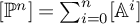
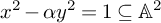
2. Let G be a one dimensional torus, defined by the vanishing set of the equation
${x^2 - \alpha y^2 = 1 \subseteq \mathbb {A}^2}$
. Then G admits a compactification isomorphic to
$\mathbb {P}^1_k$
, with complement
$\operatorname {\mathrm {Spec}}(L)$
, where
$L=k[x]/(x^2-\alpha )$
. Therefore,
$[G] = [\mathbb {P}^1] - [\operatorname {\mathrm {Spec}}(L)]$
, and since
$L/k$
is a finite étale algebra, we see that G is
$\mathrm {K}_0$
-étale linear. Similarly, any torus which is a product of
$1$
-dimensional tori is
$\mathrm {K}_0$
-étale linear. -
3. Consider
$C = \{xy=0\} \subseteq \mathbb {A}^2$
. Note that
$C \setminus \{(0,0)\} \cong \mathbb {G}_{m,k} \amalg \mathbb {G}_{m,k}$
, so we may write
$[C] = 2[\mathbb {G}_{m,k}] + [\operatorname {\mathrm {Spec}}(k)]$
, so C is
$\mathrm {K}_0$
-étale linear. -
4. Let C denote the curve
$y^2 z = x^3 \subseteq \mathbb {P}^2_{[x:y:z]}$
. We see that
$ (C \setminus \{[0:0:1]\}) \cong \mathbb {A}^1$
via the isomorphism
$[x:y:z] \mapsto \frac {x}{y}$
. Therefore
$[C] = [\mathbb {A}^1] + [\operatorname {\mathrm {Spec}}(k)]$
, so C is
$\mathrm {K}_0$
-étale linear. In particular,
$\mathrm {K}_0$
-étale linear varieties do not need to have smooth irreducible components.


Theorem 3.2. Suppose k is a field of characteristic
 $0$
. Let
$0$
. Let
 $X/k$
be a geometrically connected variety which is
$X/k$
be a geometrically connected variety which is
 $\mathrm {K}_0$
-étale linear. Then X is geometrically stably rational.
$\mathrm {K}_0$
-étale linear. Then X is geometrically stably rational.
Proof. Suppose that X is not geometrically stably rational. Let
 $\overline {k}$
be a separable closure of k. Suppose that
$\overline {k}$
be a separable closure of k. Suppose that
 $[X] \in \mathrm {K}_0(\mathrm {\acute {E}tLin}_k)$
. After base changing to
$[X] \in \mathrm {K}_0(\mathrm {\acute {E}tLin}_k)$
. After base changing to
 $\overline {k}$
, we easily see that
$\overline {k}$
, we easily see that
 ${[X_{\overline {k}}] \in \mathrm {K}_0(\mathrm {\acute {E}tLin}_{\overline {k}})}$
, and since k has characteristic
${[X_{\overline {k}}] \in \mathrm {K}_0(\mathrm {\acute {E}tLin}_{\overline {k}})}$
, and since k has characteristic
 $0$
,
$0$
,
 $\mathrm {K}^{uh}_0(\mathrm {\acute {E}tLin}_k)=\mathrm {K}_0(\mathrm {\acute {E}tLin}_k)$
, and
$\mathrm {K}^{uh}_0(\mathrm {\acute {E}tLin}_k)=\mathrm {K}_0(\mathrm {\acute {E}tLin}_k)$
, and
 $\mathrm {K}_0(\mathrm {\acute {E}tLin}_k)$
is generated by varieties of dimension
$\mathrm {K}_0(\mathrm {\acute {E}tLin}_k)$
is generated by varieties of dimension
 $0$
and the class
$0$
and the class
 $[\mathbb {A}^1]$
. Since
$[\mathbb {A}^1]$
. Since
 $\overline {k}$
is separably closed, all varieties of dimension
$\overline {k}$
is separably closed, all varieties of dimension
 $0$
are disjoint unions of
$0$
are disjoint unions of
 $\operatorname {\mathrm {Spec}}(\overline {k})$
, and therefore
$\operatorname {\mathrm {Spec}}(\overline {k})$
, and therefore
 $\mathrm {K}_0(\mathrm {\acute {E}tLin}_{\overline {k}})$
is simply the subring of
$\mathrm {K}_0(\mathrm {\acute {E}tLin}_{\overline {k}})$
is simply the subring of
 $\mathrm {K}_0(\mathrm {Var}_k)$
generated by
$\mathrm {K}_0(\mathrm {Var}_k)$
generated by
 $[\mathbb {A}^1]$
. This question therefore reduces to the case where k is separably closed.
$[\mathbb {A}^1]$
. This question therefore reduces to the case where k is separably closed.
Let I denote the ideal of
 $\mathrm {K}_0(\mathrm {Var}_{k})$
generated by
$\mathrm {K}_0(\mathrm {Var}_{k})$
generated by
 $[\mathbb {A}^1]$
. Then by a result of Larsen and Lunts [Reference Larsen and LuntsLL03, Proposition 2.7], we have an isomorphism
$[\mathbb {A}^1]$
. Then by a result of Larsen and Lunts [Reference Larsen and LuntsLL03, Proposition 2.7], we have an isomorphism
 $\mathrm {K}_0(\mathrm {Var}_k)/I \cong \mathbb {Z}[SB]$
, where
$\mathrm {K}_0(\mathrm {Var}_k)/I \cong \mathbb {Z}[SB]$
, where
 $\mathbb {Z}[SB]$
is the ring whose underlying additive group is the free abelian group generated by stable-birational classes of connected varieties. By [Reference Larsen and LuntsLL03, Proposition 2.7], a connected smooth projective variety
$\mathbb {Z}[SB]$
is the ring whose underlying additive group is the free abelian group generated by stable-birational classes of connected varieties. By [Reference Larsen and LuntsLL03, Proposition 2.7], a connected smooth projective variety
 $X/k$
is stably rational if and only if
$X/k$
is stably rational if and only if
 $[X] \in \mathrm {K}_0(\mathrm {Var}_k)$
is congruent to
$[X] \in \mathrm {K}_0(\mathrm {Var}_k)$
is congruent to
 $1 \pmod {I}$
. By assumption, X is not stably rational, so
$1 \pmod {I}$
. By assumption, X is not stably rational, so
 $[X] \neq 1 \in \mathbb {Z}[SB]$
, and X connected also means
$[X] \neq 1 \in \mathbb {Z}[SB]$
, and X connected also means
 $[X] \neq n$
for any n. This means there is no element
$[X] \neq n$
for any n. This means there is no element
 $Y \in I$
such that
$Y \in I$
such that
 $Y+n[\operatorname {\mathrm {Spec}}(k)] = [X]$
for any
$Y+n[\operatorname {\mathrm {Spec}}(k)] = [X]$
for any
 $n \in \mathbb {Z}$
. Since every element of
$n \in \mathbb {Z}$
. Since every element of
 $\mathrm {K}_0(\mathrm {\acute {E}tLin}_{\overline {k}})$
can be written in this manner,
$\mathrm {K}_0(\mathrm {\acute {E}tLin}_{\overline {k}})$
can be written in this manner,
 $[X]$
is not in
$[X]$
is not in
 $\mathrm {K}_0(\mathrm {\acute {E}tLin}_{\overline {k}})$
. This gives the result.
$\mathrm {K}_0(\mathrm {\acute {E}tLin}_{\overline {k}})$
. This gives the result.
Definition 3.2. Following [Reference LevineLev20, Page 2189], we say a variety
 $X/k$
is cellular if there exists a filtration
$X/k$
is cellular if there exists a filtration
 $$ \begin{align*}\emptyset = X_0 \subseteq X_1 \subseteq X_2 \ldots \subseteq X_n = X \end{align*} $$
such that
 $X_{i+1} \setminus X_{i}$
is a disjoint union of copies of
$X_{i+1} \setminus X_{i}$
is a disjoint union of copies of
 $\mathbb {A}^i_k$
.
$\mathbb {A}^i_k$
.
Lemma 3.3. Let
 $X/k$
be a cellular variety. Then X is
$X/k$
be a cellular variety. Then X is
 $\mathrm {K}_0$
-étale linear.
$\mathrm {K}_0$
-étale linear.
Proof. Let
 $\emptyset = X_0 \subseteq X_1 \ldots \subseteq X_n = X$
denote the filtration on X coming from its cellular structure. Let
$\emptyset = X_0 \subseteq X_1 \ldots \subseteq X_n = X$
denote the filtration on X coming from its cellular structure. Let
 $m_i$
denote the number of disjoint copies of
$m_i$
denote the number of disjoint copies of
 $\mathbb {A}^i_k$
in
$\mathbb {A}^i_k$
in
 $X_{i+1} \setminus X_i$
. In
$X_{i+1} \setminus X_i$
. In
 $\mathrm {K}_0(\mathrm {Var}_k)$
, we may write
$\mathrm {K}_0(\mathrm {Var}_k)$
, we may write
 $$ \begin{align*}[X] = \sum_{i=0}^n [ X_{i+1} \setminus X_i ] = \sum_{i=0}^n m_i[\mathbb{A}^i], \end{align*} $$
and the claim is now clear.
Remark 3.4. The curve
 $\{xy=0\}\subseteq \mathbb {A}^2$
is not cellular, even though its irreducible components are cellular and their intersection is cellular, so the class of
$\{xy=0\}\subseteq \mathbb {A}^2$
is not cellular, even though its irreducible components are cellular and their intersection is cellular, so the class of
 $\mathrm {K}_0$
-étale linear varieties is strictly larger than the class of cellular varieties.
$\mathrm {K}_0$
-étale linear varieties is strictly larger than the class of cellular varieties.
Remark 3.5. In [Reference Morel and SawantMS23, Section 2], Morel and Sawant use a more general definition of cellular varieties by relaxing the condition on the stratification so that we only require that
 $X_{i+1} \setminus X_i$
is a disjoint union of cohomologically trivial varieties. Using this definition,
$X_{i+1} \setminus X_i$
is a disjoint union of cohomologically trivial varieties. Using this definition,
 $\mathbb {A}^1$
-contractible varieties are cellular, e.g. Hoyois, Krishna and Østvær have proven that Koras–Russell threefolds are
$\mathbb {A}^1$
-contractible varieties are cellular, e.g. Hoyois, Krishna and Østvær have proven that Koras–Russell threefolds are
 $\mathbb {A}^1$
-contractible [Reference Hoyois, Krishna and Arne ØstværHKØ16] so these are “cellular” in the sense of [Reference Morel and SawantMS23]. However, the subtle nature of the ring
$\mathbb {A}^1$
-contractible [Reference Hoyois, Krishna and Arne ØstværHKØ16] so these are “cellular” in the sense of [Reference Morel and SawantMS23]. However, the subtle nature of the ring
 $\mathrm {K}_0(\mathrm {Var}_k)$
means that it is unclear to the authors whether such varieties are
$\mathrm {K}_0(\mathrm {Var}_k)$
means that it is unclear to the authors whether such varieties are
 $\mathrm {K}_0$
-étale linear.
$\mathrm {K}_0$
-étale linear.
Definition 3.3. Following Section 3 of Totaro’s paper [Reference TotaroTot14] and [Reference JoshuaJos01, Section 2], we say a variety X over k is 0-linear if it is isomorphic to
 $\mathbb {A}^m_k$
for some
$\mathbb {A}^m_k$
for some
 $m \in \mathbb {N}$
. A variety X over k is n-linear for
$m \in \mathbb {N}$
. A variety X over k is n-linear for
 $n \geq 1$
if there exists an open embedding
$n \geq 1$
if there exists an open embedding
 $U \rightarrow V$
with complement Z, such that
$U \rightarrow V$
with complement Z, such that
 $X \in \{U,V,Z\}$
and the other two are
$X \in \{U,V,Z\}$
and the other two are
 $(n-1)$
-linear. A variety X over k is linear if it is n-linear for some
$(n-1)$
-linear. A variety X over k is linear if it is n-linear for some
 $n \in \mathbb {N}$
.
$n \in \mathbb {N}$
.
The class of linear varieties includes any variety which admits a stratification into linear varieties. In particular, it includes all projective spaces, Grassmannians, flag varieties, and blowups of projective spaces in linear subvarieties. It is easy to see that all linear varieties are
 $\mathrm {K}_0$
-étale linear.
$\mathrm {K}_0$
-étale linear.
Remark 3.6. The class of
 $\mathrm {K}_0$
-étale linear varieties is strictly bigger than the class of linear varieties. For example, when
$\mathrm {K}_0$
-étale linear varieties is strictly bigger than the class of linear varieties. For example, when
 $L/k$
is a quadratic field extension,
$L/k$
is a quadratic field extension,
 $\operatorname {\mathrm {Spec}}(L)$
does not admit a stratification as in Definition 3.3.
$\operatorname {\mathrm {Spec}}(L)$
does not admit a stratification as in Definition 3.3.
When k is separably closed and characteristic
 $0$
, the class of
$0$
, the class of
 $\mathrm {K}_0$
-étale linear varieties are those whose class in
$\mathrm {K}_0$
-étale linear varieties are those whose class in
 $\mathrm {K}_0(\mathrm {Var}_k)$
lie in the subring generated by
$\mathrm {K}_0(\mathrm {Var}_k)$
lie in the subring generated by
 $\mathbb {A}^1$
. Clearly all linear varieties lie in this subring. It is unclear if all
$\mathbb {A}^1$
. Clearly all linear varieties lie in this subring. It is unclear if all
 $\mathrm {K}_0$
-étale linear varieties over a separably closed field are linear. That is, even in characteristic
$\mathrm {K}_0$
-étale linear varieties over a separably closed field are linear. That is, even in characteristic
 $0$
, there may exist varieties
$0$
, there may exist varieties
 $X/k$
that do not admit stratifications as above, but nevertheless the class
$X/k$
that do not admit stratifications as above, but nevertheless the class
 $[X]$
lies in
$[X]$
lies in
 $\mathrm {K}_0(\mathrm {\acute {E}tLin}_k)$
.
$\mathrm {K}_0(\mathrm {\acute {E}tLin}_k)$
.
The class of
 $\mathrm {K}_0$
-étale linear varieties is closed under natural geometric constructions: clearly they are closed under products and scissor relations, but we also have the following.
$\mathrm {K}_0$
-étale linear varieties is closed under natural geometric constructions: clearly they are closed under products and scissor relations, but we also have the following.
Lemma 3.7. Let X be
 $\mathrm {K}_0$
-étale linear, and let
$\mathrm {K}_0$
-étale linear, and let
 $p: E \rightarrow X$
be a Zariski locally trivial fibre bundle whose fibre F is
$p: E \rightarrow X$
be a Zariski locally trivial fibre bundle whose fibre F is
 $\mathrm {K}_0$
-étale linear. Then E is
$\mathrm {K}_0$
-étale linear. Then E is
 $\mathrm {K}_0$
-étale linear.
$\mathrm {K}_0$
-étale linear.
Proof. Since
 $E \to X$
is Zariski locally trivialisable, we see
$E \to X$
is Zariski locally trivialisable, we see
 $[E] = [X][F]$
for example by Remark 4.1 of [Reference GöttscheGöt01]. Since
$[E] = [X][F]$
for example by Remark 4.1 of [Reference GöttscheGöt01]. Since
 $\mathrm {K}_0(\mathrm {\acute {E}tLin}_k)$
is a ring and
$\mathrm {K}_0(\mathrm {\acute {E}tLin}_k)$
is a ring and
 $[X], [F] \in \mathrm {K}_0(\mathrm {\acute {E}tLin}_k)$
by assumption, the result follows.
$[X], [F] \in \mathrm {K}_0(\mathrm {\acute {E}tLin}_k)$
by assumption, the result follows.
Lemma 3.8. Let X be a smooth variety, and let Z be a smooth closed subvariety of X such that Z is
 $\mathrm {K}_0$
-étale linear. Then the blow up
$\mathrm {K}_0$
-étale linear. Then the blow up
 $\mathrm {Bl}_Z(X)$
is
$\mathrm {Bl}_Z(X)$
is
 $\mathrm {K}_0$
-étale linear if and only if X is
$\mathrm {K}_0$
-étale linear if and only if X is
 $\mathrm {K}_0$
-étale linear.
$\mathrm {K}_0$
-étale linear.
Proof. Let
 $Y := \mathrm {Bl}_Z(X)$
and let E denote the exceptional divisor of the blow up. Note that
$Y := \mathrm {Bl}_Z(X)$
and let E denote the exceptional divisor of the blow up. Note that
 $[Z] \in \mathrm {K}_0(\mathrm {\acute {E}tLin}_k)$
. As
$[Z] \in \mathrm {K}_0(\mathrm {\acute {E}tLin}_k)$
. As
 $Z \rightarrow X$
is a regular closed immersion, E is given by the projectivisation of the conormal bundle
$Z \rightarrow X$
is a regular closed immersion, E is given by the projectivisation of the conormal bundle
 $\mathcal {N}_{Z/X}$
and is therefore a projective bundle over Z. It follows from Lemma 3.7 that
$\mathcal {N}_{Z/X}$
and is therefore a projective bundle over Z. It follows from Lemma 3.7 that
 $[E] \in \mathrm {K}_0(\mathrm {\acute {E}tLin}_k)$
. By Bittner’s theorem [Reference BittnerBit04, Theorem 3.1], we see that
$[E] \in \mathrm {K}_0(\mathrm {\acute {E}tLin}_k)$
. By Bittner’s theorem [Reference BittnerBit04, Theorem 3.1], we see that
 $$ \begin{align*}[X] - [Z] = [X\setminus Z] = [Y\setminus E] = [Y] - [E] \in \mathrm{K}_0(\mathrm{Var}_k), \end{align*} $$
and therefore
 $[Y] \in \mathrm {K}_0(\mathrm {\acute {E}tLin}_k)$
if and only if
$[Y] \in \mathrm {K}_0(\mathrm {\acute {E}tLin}_k)$
if and only if
 $[X] \in \mathrm {K}_0(\mathrm {\acute {E}tLin}_k)$
, since
$[X] \in \mathrm {K}_0(\mathrm {\acute {E}tLin}_k)$
, since
 $\mathrm {K}_0(\mathrm {\acute {E}tLin}_k)$
forms a subring of
$\mathrm {K}_0(\mathrm {\acute {E}tLin}_k)$
forms a subring of
 $\mathrm {K}_0(\mathrm {Var}_{k})$
.
$\mathrm {K}_0(\mathrm {Var}_{k})$
.
4 Symmetrisable varieties
In this section, we prove the main result of this paper, namely that
 $\mathrm {K}_0$
-étale linear varieties are symmetrisable, see Definition 4.1. We also show that the subset of classes of
$\mathrm {K}_0$
-étale linear varieties are symmetrisable, see Definition 4.1. We also show that the subset of classes of
 $K_0(\mathrm {Var}_k)$
which are compatible with the power structures,
$K_0(\mathrm {Var}_k)$
which are compatible with the power structures,
 $\mathrm {K}_0(\mathrm {Sym}_k)$
, is a
$\mathrm {K}_0(\mathrm {Sym}_k)$
, is a
 $\mathrm {K}_0(\mathrm {\acute {E}tLin}_k)$
-submodule of
$\mathrm {K}_0(\mathrm {\acute {E}tLin}_k)$
-submodule of
 $\mathrm {K}_0(\mathrm {Var}_{k})$
.
$\mathrm {K}_0(\mathrm {Var}_{k})$
.
4.1 Properties of symmetrisable varieties
Definition 4.1. A variety X is symmetrisable if
 $\chi _c^{\mathrm {mot}}(X^{(m)}) = a_m (\chi _c^{\mathrm {mot}}(X))$
for all m. Let
$\chi _c^{\mathrm {mot}}(X^{(m)}) = a_m (\chi _c^{\mathrm {mot}}(X))$
for all m. Let
 $\mathrm {Sym}_k \subset \mathrm {Var}_k$
be the full subcategory consisting of symmetrisable varieties.
$\mathrm {Sym}_k \subset \mathrm {Var}_k$
be the full subcategory consisting of symmetrisable varieties.
Informally, symmetrisable varieties are varieties that are compatible with our power structures on
 $\mathrm {K}_0(\mathrm {Var}_{k})$
and
$\mathrm {K}_0(\mathrm {Var}_{k})$
and
 $\operatorname {\mathrm {GW}}(k)$
under the morphism
$\operatorname {\mathrm {GW}}(k)$
under the morphism
 $\chi _c^{\mathrm {mot}}$
.
$\chi _c^{\mathrm {mot}}$
.
Definition 4.2. Let
 $\mathrm {K}^{uh}_0(\mathrm {Sym}_k)$
be the subset of
$\mathrm {K}^{uh}_0(\mathrm {Sym}_k)$
be the subset of
 $\mathrm {K}_0^{uh}(\mathrm {Var}_k)$
consisting of elements s such that
$\mathrm {K}_0^{uh}(\mathrm {Var}_k)$
consisting of elements s such that
 $\chi _c^{\mathrm {mot}}(S_m (s)) = a_m (\chi _c^{\mathrm {mot}}(s))$
for all
$\chi _c^{\mathrm {mot}}(S_m (s)) = a_m (\chi _c^{\mathrm {mot}}(s))$
for all
 $m \in \mathbb {Z}_{\geq 0}$
, where
$m \in \mathbb {Z}_{\geq 0}$
, where
 $S_m$
is the power structure on
$S_m$
is the power structure on
 $\mathrm {K}_0(\mathrm {Var}_{k})$
induced by symmetric powers as in Definition 2.6. It is an abelian subgroup of
$\mathrm {K}_0(\mathrm {Var}_{k})$
induced by symmetric powers as in Definition 2.6. It is an abelian subgroup of
 $\mathrm {K}_0(\mathrm {Var}_{k})$
by [Reference Pajwani and PálPP25, Lemma 2.9]. Define
$\mathrm {K}_0(\mathrm {Var}_{k})$
by [Reference Pajwani and PálPP25, Lemma 2.9]. Define
 $\mathrm {K}_0(\mathrm {Sym}_k)$
to be the preimage of
$\mathrm {K}_0(\mathrm {Sym}_k)$
to be the preimage of
 $\mathrm {K}_0^{uh}(\mathrm {Var}_k)$
under the natural quotient
$\mathrm {K}_0^{uh}(\mathrm {Var}_k)$
under the natural quotient
 $\mathrm {K}_0(\mathrm {Var}_k) \to \mathrm {K}_0^{uh}(\mathrm {Var}_k)$
.
$\mathrm {K}_0(\mathrm {Var}_k) \to \mathrm {K}_0^{uh}(\mathrm {Var}_k)$
.
Note that a variety X is symmetrisable if and only if
 $[X] \in \mathrm {K}_0(\mathrm {Sym}_k)$
, and we later see in Corollary 4.9 that
$[X] \in \mathrm {K}_0(\mathrm {Sym}_k)$
, and we later see in Corollary 4.9 that
 $\mathrm {K}_0(\mathrm {Sym}_k)$
is the sub-abelian group of
$\mathrm {K}_0(\mathrm {Sym}_k)$
is the sub-abelian group of
 $\mathrm {K}_0(\mathrm {Var}_{k})$
generated by symmetrisable varieties, at least in characteristic
$\mathrm {K}_0(\mathrm {Var}_{k})$
generated by symmetrisable varieties, at least in characteristic
 $0$
.
$0$
.
This paper studies the structure of
 $\mathrm {K}_0(\mathrm {Sym}_k) \subseteq \mathrm {K}_0(\mathrm {Var}_k)$
, so can be thought of as a geometric extension of the purely arithmetic results of [Reference Pajwani and PálPP25]. Indeed, [Reference Pajwani and PálPP25, Corollary 4.30] shows that
$\mathrm {K}_0(\mathrm {Sym}_k) \subseteq \mathrm {K}_0(\mathrm {Var}_k)$
, so can be thought of as a geometric extension of the purely arithmetic results of [Reference Pajwani and PálPP25]. Indeed, [Reference Pajwani and PálPP25, Corollary 4.30] shows that
 $\mathrm {Sym}_k$
contains all zero-dimensional varieties, so
$\mathrm {Sym}_k$
contains all zero-dimensional varieties, so
 $\mathrm {K}_0(\mathrm {\acute {E}t}_k) \subseteq \mathrm {K}_0(\mathrm {Sym}_k)$
. A slight modification of the arguments in [Reference Pajwani and PálPP25] gives us the following.
$\mathrm {K}_0(\mathrm {\acute {E}t}_k) \subseteq \mathrm {K}_0(\mathrm {Sym}_k)$
. A slight modification of the arguments in [Reference Pajwani and PálPP25] gives us the following.
Theorem 4.1. Let X be symmetrisable. Then
 $X \times _k \operatorname {\mathrm {Spec}}(A)$
is symmetrisable for any finite étale algebra
$X \times _k \operatorname {\mathrm {Spec}}(A)$
is symmetrisable for any finite étale algebra
 $A/k$
.
$A/k$
.
Proof. This follows by an identical argument to [Reference Pajwani and PálPP25, Subsection 4.3], which we sketch here for convenience. By [Reference Pajwani and PálPP25, Corollary 4.24], X is symmetrisable implies that
 $X \times _k \operatorname {\mathrm {Spec}}(K)$
is also symmetrisable for
$X \times _k \operatorname {\mathrm {Spec}}(K)$
is also symmetrisable for
 $\mathrm {K}/k$
a quadratic étale algebra. By repeatedly applying this result, we see that for any multiquadratic étale algebra
$\mathrm {K}/k$
a quadratic étale algebra. By repeatedly applying this result, we see that for any multiquadratic étale algebra
 $A/k$
, the product
$A/k$
, the product
 $X \times _k \operatorname {\mathrm {Spec}}(A)$
is also symmetrisable. As in [Reference Pajwani and PálPP25, Lemma 4.27], for any positive integer n the assignments
$X \times _k \operatorname {\mathrm {Spec}}(A)$
is also symmetrisable. As in [Reference Pajwani and PálPP25, Lemma 4.27], for any positive integer n the assignments
 $A \mapsto a_n(\chi _c^{\mathrm {mot}}(X \times _k A))$
and
$A \mapsto a_n(\chi _c^{\mathrm {mot}}(X \times _k A))$
and
 $A \mapsto \chi _c^{\mathrm {mot}}((X \times _k A)^{(n)})$
both define invariants valued in the Witt ring
$A \mapsto \chi _c^{\mathrm {mot}}((X \times _k A)^{(n)})$
both define invariants valued in the Witt ring
 $W(k) = \operatorname {\mathrm {GW}}(k)/(\mathbb {H})$
, and the above shows they take the same values whenever A is a multiquadratic étale algebra, so the result [Reference Garibaldi, Merkurjev and SerreGMS03, Theorem 29.1] of Garibaldi, Merkurjev and Serre together with the observation that the ranks are the same gives the result, i.e.
$W(k) = \operatorname {\mathrm {GW}}(k)/(\mathbb {H})$
, and the above shows they take the same values whenever A is a multiquadratic étale algebra, so the result [Reference Garibaldi, Merkurjev and SerreGMS03, Theorem 29.1] of Garibaldi, Merkurjev and Serre together with the observation that the ranks are the same gives the result, i.e.
 $X \times _k \operatorname {\mathrm {Spec}}(A)$
is symmetrisable.
$X \times _k \operatorname {\mathrm {Spec}}(A)$
is symmetrisable.
Corollary 4.2. The group
 $\mathrm {K}_0(\mathrm {Sym}_k)$
is a
$\mathrm {K}_0(\mathrm {Sym}_k)$
is a
 $\mathrm {K}_0(\mathrm {\acute {E}t}_k)$
-submodule of
$\mathrm {K}_0(\mathrm {\acute {E}t}_k)$
-submodule of
 $\mathrm {K}_0(\mathrm {Var}_{k})$
.
$\mathrm {K}_0(\mathrm {Var}_{k})$
.
Proof. Note that
 $\mathrm {K}_0(\mathrm {Sym}_k)$
is a
$\mathrm {K}_0(\mathrm {Sym}_k)$
is a
 $\mathrm {K}_0(\mathrm {\acute {E}t}_k)$
-module if and only if for all symmetrisable varieties X and finite separable field extensions
$\mathrm {K}_0(\mathrm {\acute {E}t}_k)$
-module if and only if for all symmetrisable varieties X and finite separable field extensions
 $L/k$
,
$L/k$
,
 $[\operatorname {\mathrm {Spec}}(L)] [X] \in \mathrm {K}_0(\mathrm {Sym}_k)$
, which is precisely the above theorem.
$[\operatorname {\mathrm {Spec}}(L)] [X] \in \mathrm {K}_0(\mathrm {Sym}_k)$
, which is precisely the above theorem.
Remark 4.3. It is an open question to determine whether
 $\mathrm {K}_0(\mathrm {Sym}_k) = \mathrm {K}_0(\mathrm {Var}_k)$
. For some base fields k, it is true that
$\mathrm {K}_0(\mathrm {Sym}_k) = \mathrm {K}_0(\mathrm {Var}_k)$
. For some base fields k, it is true that
 $\mathrm {K}_0(\mathrm {Sym}_k)=\mathrm {K}_0(\mathrm {Var}_k)$
. When
$\mathrm {K}_0(\mathrm {Sym}_k)=\mathrm {K}_0(\mathrm {Var}_k)$
. When
 $k=\mathbb {C}$
, there is a canonical isomorphism
$k=\mathbb {C}$
, there is a canonical isomorphism
 $\operatorname {\mathrm {GW}}(\mathbb {C}) \cong \mathbb {Z}$
and [Reference LevineLev20, Remark 2.3.1] allows us to compute
$\operatorname {\mathrm {GW}}(\mathbb {C}) \cong \mathbb {Z}$
and [Reference LevineLev20, Remark 2.3.1] allows us to compute
 $\chi _c^{\mathrm {mot}}(X) = e_c(X(\mathbb {C}))$
, where
$\chi _c^{\mathrm {mot}}(X) = e_c(X(\mathbb {C}))$
, where
 $e_c$
denotes the compactly supported Euler characteristic of the topological space
$e_c$
denotes the compactly supported Euler characteristic of the topological space
 $X(\mathbb {C})$
. We may then apply MacDonald’s Theorem ([Reference MacdonaldMac62b]) to obtain
$X(\mathbb {C})$
. We may then apply MacDonald’s Theorem ([Reference MacdonaldMac62b]) to obtain
 $\chi _c^{\mathrm {mot}}(X^{(n)}) = a_n(\chi _c^{\mathrm {mot}}(X))$
, so when
$\chi _c^{\mathrm {mot}}(X^{(n)}) = a_n(\chi _c^{\mathrm {mot}}(X))$
, so when
 $k=\mathbb {C}$
, we have
$k=\mathbb {C}$
, we have
 $\mathrm {K}_0(\mathrm {Sym}_{\mathbb {C}}) = \mathrm {K}_0(\mathrm {Var}_{\mathbb {C}})$
, and we may argue as in [Reference Pajwani and PálPPa, Theorem 2.14] to show the same is true when k is algebraically closed in characteristic
$\mathrm {K}_0(\mathrm {Sym}_{\mathbb {C}}) = \mathrm {K}_0(\mathrm {Var}_{\mathbb {C}})$
, and we may argue as in [Reference Pajwani and PálPPa, Theorem 2.14] to show the same is true when k is algebraically closed in characteristic
 $0$
. Similarly, when
$0$
. Similarly, when
 $k=\mathbb {R}$
, [Reference LevineLev20, Remark 2.3.1] gives
$k=\mathbb {R}$
, [Reference LevineLev20, Remark 2.3.1] gives
 $$ \begin{align*} \mathrm{sign}(\chi_c^{\mathrm{mot}}(X)) = e_c(X(\mathbb{R})). \end{align*} $$
We may then apply MacDonald’s theorem ([Reference MacdonaldMac62b]) and [Reference McGarraghyMcG05, Proposition 4.14] to see
 $\mathrm {K}_0(\mathrm {Sym}_{\mathbb {R}}) = \mathrm {K}_0(\mathrm {Var}_{\mathbb {R}})$
. Moreover, we may argue as in [Reference Pajwani and PálPPa, Theorem 2.20] to obtain the same result whenever k is a real closed field. If we let J denote the kernel of the rank, signature and discriminant morphisms out of
$\mathrm {K}_0(\mathrm {Sym}_{\mathbb {R}}) = \mathrm {K}_0(\mathrm {Var}_{\mathbb {R}})$
. Moreover, we may argue as in [Reference Pajwani and PálPPa, Theorem 2.20] to obtain the same result whenever k is a real closed field. If we let J denote the kernel of the rank, signature and discriminant morphisms out of
 $\operatorname {\mathrm {GW}}(k)$
, then [Reference Pajwani and PálPPa, Corollary 8.21] guarantees that for
$\operatorname {\mathrm {GW}}(k)$
, then [Reference Pajwani and PálPPa, Corollary 8.21] guarantees that for
 $\mathrm {char}(k)=0$
, these power structures are compatible modulo the ideal J. In particular,
$\mathrm {char}(k)=0$
, these power structures are compatible modulo the ideal J. In particular,
 $\mathrm {K}_0(\mathrm {Sym}_k) = \mathrm {K}_0(\mathrm {Var}_k)$
for all fields such that
$\mathrm {K}_0(\mathrm {Sym}_k) = \mathrm {K}_0(\mathrm {Var}_k)$
for all fields such that
 $J=0$
, which are precisely fields k such that the
$J=0$
, which are precisely fields k such that the
 $2$
-primary virtual cohomological dimension
$2$
-primary virtual cohomological dimension
 $\mathrm {vcd}_2(k) \leq 1$
by the
$\mathrm {vcd}_2(k) \leq 1$
by the
 $n=2, l=2$
case of the Milnor Conjecture, see the result [Reference MerkurjevMer81, Theorem 2.2] of Merkurjev. For this class of fields, the map
$n=2, l=2$
case of the Milnor Conjecture, see the result [Reference MerkurjevMer81, Theorem 2.2] of Merkurjev. For this class of fields, the map
 $$ \begin{align*} - \cup [2]: H^1(k, \mathbb{Z}/2\mathbb{Z}) \longrightarrow H^2(k, \mathbb{Z}/2\mathbb{Z}) \end{align*} $$
is zero. In particular, in every known example where
 $\mathrm {K}_0(\mathrm {Var}_k) = \mathrm {K}_0(\mathrm {Sym}_k)$
, the power structure on
$\mathrm {K}_0(\mathrm {Var}_k) = \mathrm {K}_0(\mathrm {Sym}_k)$
, the power structure on
 $\operatorname {\mathrm {GW}}(k)$
from Definition 2.4 agrees with the non factorial symmetric power structure of [Reference McGarraghyMcG05]. It is unknown whether the non-vanishing of this map provides an obstruction to the compatibility of these power structures, and if so, whether this obstruction would be the only one to this compatibility.
$\operatorname {\mathrm {GW}}(k)$
from Definition 2.4 agrees with the non factorial symmetric power structure of [Reference McGarraghyMcG05]. It is unknown whether the non-vanishing of this map provides an obstruction to the compatibility of these power structures, and if so, whether this obstruction would be the only one to this compatibility.
4.2 Göttsche’s lemma for symmetric powers
In this section, we will prove Theorem 4.8 using Göttsche’s Lemma for symmetric powers. The following appears as the second half of [Reference GöttscheGöt01, Lemma 4.4], being a corollary of the first half. For a detailed account of Göttsche’s Lemma and its proof, we refer the reader to [Reference Chambert-Loir, Nicaise and SebagCLNS18, Proposition 1.1.11 in Chapter 7].
Corollary 4.4. Let X be a variety over k and let
 $l,n \in \mathbb {N}$
. Then in
$l,n \in \mathbb {N}$
. Then in
 $\mathrm {K}_0^{uh}(\mathrm {Var}_k)$
, we have
$\mathrm {K}_0^{uh}(\mathrm {Var}_k)$
, we have
 $[(X \times \mathbb {A}^l)^{(n)}] = [X^{(n)} \times \mathbb {A}^{nl}]$
.
$[(X \times \mathbb {A}^l)^{(n)}] = [X^{(n)} \times \mathbb {A}^{nl}]$
.
Remark 4.5. For
 $X=\operatorname {\mathrm {Spec}}(k)$
and
$X=\operatorname {\mathrm {Spec}}(k)$
and
 $l=1$
, Corollary 4.4 can be proven in an elementary way. By the fundamental theorem of symmetric polynomials and the definition of the symmetric power of an affine variety, we have
$l=1$
, Corollary 4.4 can be proven in an elementary way. By the fundamental theorem of symmetric polynomials and the definition of the symmetric power of an affine variety, we have
 $$ \begin{align*} (\mathbb{A}^1)^{(n)} = \operatorname{\mathrm{Spec}}(k[x_1, \dots, x_n]^{S_n}) = \operatorname{\mathrm{Spec}}(k[e_1, \dots, e_n]) = \mathbb{A}^n. \end{align*} $$
Here, the
 $e_i$
are the elementary symmetric polynomials in the variables
$e_i$
are the elementary symmetric polynomials in the variables
 $x_i$
.
$x_i$
.
Using Göttsche’s result above, we may quickly deduce the following.
Corollary 4.6. There is an equality
 $[(\mathbb {A}^m)^{(n)}] = [\mathbb {A}^{mn}]$
in
$[(\mathbb {A}^m)^{(n)}] = [\mathbb {A}^{mn}]$
in
 $\mathrm {K}_0^{uh}(\mathrm {Var}_k)$
.
$\mathrm {K}_0^{uh}(\mathrm {Var}_k)$
.
Proof. Immediate, by taking
 $X=\operatorname {\mathrm {Spec}}(k)$
in the above Corollary.
$X=\operatorname {\mathrm {Spec}}(k)$
in the above Corollary.
Corollary 4.7. If X is a
 $\mathrm {K}_0$
-étale linear variety, then
$\mathrm {K}_0$
-étale linear variety, then
 $X^{(n)}$
is
$X^{(n)}$
is
 $\mathrm {K}_0$
-étale linear.
$\mathrm {K}_0$
-étale linear.
Proof. For
 $[X]=[\mathbb {A}^n]$
, this is immediate by the above. For
$[X]=[\mathbb {A}^n]$
, this is immediate by the above. For
 $[X] = [\operatorname {\mathrm {Spec}}(L) \times \mathbb {A}^n]$
where
$[X] = [\operatorname {\mathrm {Spec}}(L) \times \mathbb {A}^n]$
where
 $L/k$
is a finite étale algebra, this follows by Corollary 4.4. For a general variety X with
$L/k$
is a finite étale algebra, this follows by Corollary 4.4. For a general variety X with
 $[X] \in \mathrm {K}_0(\mathrm {\acute {E}tLin}_k)$
this follows since after passing to the quotient in
$[X] \in \mathrm {K}_0(\mathrm {\acute {E}tLin}_k)$
this follows since after passing to the quotient in
 $\mathrm {K}^{uh}_0(\mathrm {Var}_k)$
we can write
$\mathrm {K}^{uh}_0(\mathrm {Var}_k)$
we can write
 $[X] = \sum _i m_i [\operatorname {\mathrm {Spec}}(L_i)] [\mathbb {A}^i]$
. This then follows by applying the formulae for the functions defining power structures from Definition 2.4.
$[X] = \sum _i m_i [\operatorname {\mathrm {Spec}}(L_i)] [\mathbb {A}^i]$
. This then follows by applying the formulae for the functions defining power structures from Definition 2.4.
Theorem 4.8. Let X be a
 $\mathrm {K}_0$
-étale linear variety over k. Then X is symmetrisable.
$\mathrm {K}_0$
-étale linear variety over k. Then X is symmetrisable.
Proof. Recall that
 $\chi _c^{\mathrm {mot}}(\mathbb {A}^{m}) = \langle (-1)^m \rangle $
. Then by Corollary 4.6 and Lemma 2.8 we have
$\chi _c^{\mathrm {mot}}(\mathbb {A}^{m}) = \langle (-1)^m \rangle $
. Then by Corollary 4.6 and Lemma 2.8 we have
 $$ \begin{align*} \chi_c^{\mathrm{mot}}((\mathbb{A}^m)^{(n)}) = \chi_c^{\mathrm{mot}}( \mathbb{A}^{mn}) = \langle (-1)^{mn} \rangle = a_n(\langle (-1)^m \rangle), \end{align*} $$
where we use that
 $\chi _c^{\mathrm {mot}}(\mathbb {A}^1) = \langle -1 \rangle $
. Therefore,
$\chi _c^{\mathrm {mot}}(\mathbb {A}^1) = \langle -1 \rangle $
. Therefore,
 $\mathbb {A}^d$
is symmetrisable. Corollary 4.2 then tells us that
$\mathbb {A}^d$
is symmetrisable. Corollary 4.2 then tells us that
 $[\mathbb {A}^d]\cdot [\operatorname {\mathrm {Spec}}(L)]$
is symmetrisable for any
$[\mathbb {A}^d]\cdot [\operatorname {\mathrm {Spec}}(L)]$
is symmetrisable for any
 $L/k$
a finite separable field extension. Since
$L/k$
a finite separable field extension. Since
 $\mathrm {K}_0(\mathrm {Sym}_k)$
is a finite abelian subgroup of
$\mathrm {K}_0(\mathrm {Sym}_k)$
is a finite abelian subgroup of
 $\mathrm {K}_0(\mathrm {Var}_k)$
, any variety X such that
$\mathrm {K}_0(\mathrm {Var}_k)$
, any variety X such that
 ${[X] = \sum _{i=0}^n m_i [\mathbb {A}^i] [\operatorname {\mathrm {Spec}}(L_i)]}$
is also symmetrisable, which are all
${[X] = \sum _{i=0}^n m_i [\mathbb {A}^i] [\operatorname {\mathrm {Spec}}(L_i)]}$
is also symmetrisable, which are all
 $\mathrm {K}_0$
-étale linear varieties by Definition 3.1.
$\mathrm {K}_0$
-étale linear varieties by Definition 3.1.
Corollary 4.9. When k has characteristic
 $0$
, the abelian group
$0$
, the abelian group
 $\mathrm {K}_0(\mathrm {Sym}_k)$
is the abelian subgroup of
$\mathrm {K}_0(\mathrm {Sym}_k)$
is the abelian subgroup of
 $\mathrm {K}_0(\mathrm {Var}_{k})$
generated by classes of symmetrisable varieties.
$\mathrm {K}_0(\mathrm {Var}_{k})$
generated by classes of symmetrisable varieties.
Proof. Let
 $s \in \mathrm {K}_0(\mathrm {Sym}_k)$
. Since we are in characteristic
$s \in \mathrm {K}_0(\mathrm {Sym}_k)$
. Since we are in characteristic
 $0$
, we may apply Bittner’s Theorem [Reference BittnerBit04, Theorem 3.1], to see that
$0$
, we may apply Bittner’s Theorem [Reference BittnerBit04, Theorem 3.1], to see that
 $\mathrm {K}_0(\mathrm {Var}_k)$
is generated as an abelian group by smooth projective varieties. We may therefore write
$\mathrm {K}_0(\mathrm {Var}_k)$
is generated as an abelian group by smooth projective varieties. We may therefore write
 $s = [X] - [Y]$
where both X and Y are smooth projective varieties.
$s = [X] - [Y]$
where both X and Y are smooth projective varieties.
Since Y is projective, it admits a closed embedding
 $Y \hookrightarrow \mathbb {P}^m$
for some m. Define
$Y \hookrightarrow \mathbb {P}^m$
for some m. Define
 $U := \mathbb {P}^m \setminus Y$
. Then
$U := \mathbb {P}^m \setminus Y$
. Then
 $s + [\mathbb {P}^m] = [X] + [\mathbb {P}^m] - [Y] = [X] + [U] = [X \amalg U]$
. Since
$s + [\mathbb {P}^m] = [X] + [\mathbb {P}^m] - [Y] = [X] + [U] = [X \amalg U]$
. Since
 $\mathbb {P}^m$
is
$\mathbb {P}^m$
is
 $\mathrm {K}_0$
-étale linear, it is symmetrisable by the above theorem. Therefore, since
$\mathrm {K}_0$
-étale linear, it is symmetrisable by the above theorem. Therefore, since
 $\mathrm {K}_0(\mathrm {Sym}_k)$
is closed under addition, we see that
$\mathrm {K}_0(\mathrm {Sym}_k)$
is closed under addition, we see that
 $s + [\mathbb {P}^m]$
lies in
$s + [\mathbb {P}^m]$
lies in
 $\mathrm {K}_0(\mathrm {Sym}_k)$
. In particular,
$\mathrm {K}_0(\mathrm {Sym}_k)$
. In particular,
 $X \amalg U$
is a symmetrisable variety, since
$X \amalg U$
is a symmetrisable variety, since
 $[X \amalg U] = s + [\mathbb {P}^m] \in \mathrm {K}_0(\mathrm {Sym}_k)$
. Rewriting
$[X \amalg U] = s + [\mathbb {P}^m] \in \mathrm {K}_0(\mathrm {Sym}_k)$
. Rewriting
 $s = [X \amalg U] - [\mathbb {P}^m]$
shows that s can be written as a linear combination of the classes of symmetrisable varieties, as required.
$s = [X \amalg U] - [\mathbb {P}^m]$
shows that s can be written as a linear combination of the classes of symmetrisable varieties, as required.
Corollary 4.10. The subset
 $\mathrm {K}_0(\mathrm {Sym}_k)$
is a
$\mathrm {K}_0(\mathrm {Sym}_k)$
is a
 $\mathrm {K}_0(\mathrm {\acute {E}tLin}_k)$
-submodule of
$\mathrm {K}_0(\mathrm {\acute {E}tLin}_k)$
-submodule of
 $\mathrm {K}_0(\mathrm {Var}_{k})$
.
$\mathrm {K}_0(\mathrm {Var}_{k})$
.
Proof. Note that
 $\mathrm {K}_0(\mathrm {Sym}_k)$
and
$\mathrm {K}_0(\mathrm {Sym}_k)$
and
 $\mathrm {K}_0(\mathrm {\acute {E}tLin}_k)$
are both defined to be the preimages of subrings in
$\mathrm {K}_0(\mathrm {\acute {E}tLin}_k)$
are both defined to be the preimages of subrings in
 $\mathrm {K}_0^{uh}(\mathrm {\acute {E}tLin}_k)$
, so we may instead show that
$\mathrm {K}_0^{uh}(\mathrm {\acute {E}tLin}_k)$
, so we may instead show that
 $\mathrm {K}_0^{uh}(\mathrm {Sym}_k)$
is a
$\mathrm {K}_0^{uh}(\mathrm {Sym}_k)$
is a
 $\mathrm {K}_0^{uh}(\mathrm {\acute {E}tLin}_k)$
submodule of
$\mathrm {K}_0^{uh}(\mathrm {\acute {E}tLin}_k)$
submodule of
 $\mathrm {K}_0^{uh}(\mathrm {Var}_k)$
, and obtain the theorem by pulling back the result.
$\mathrm {K}_0^{uh}(\mathrm {Var}_k)$
, and obtain the theorem by pulling back the result.
Let
 $X \in \mathrm {K}^{uh}_0(\mathrm {Sym}_k)$
. Note that
$X \in \mathrm {K}^{uh}_0(\mathrm {Sym}_k)$
. Note that
 $\chi _c^{\mathrm {mot}}(X \times [\mathbb {A}^l]) = \langle (-1)^l \rangle \chi _c^{\mathrm {mot}}(X)$
by multiplicativity of
$\chi _c^{\mathrm {mot}}(X \times [\mathbb {A}^l]) = \langle (-1)^l \rangle \chi _c^{\mathrm {mot}}(X)$
by multiplicativity of
 $\chi _c^{\mathrm {mot}}$
. Corollary 4.4 gives us
$\chi _c^{\mathrm {mot}}$
. Corollary 4.4 gives us
 $$ \begin{align*}\chi_c^{\mathrm{mot}}( S_n(X \cdot [\mathbb{A}^l])) = \chi_c^{\mathrm{mot}}(S_n(X) \cdot [\mathbb{A}^{ln}]) = \langle (-1)^{ln} \rangle a_n(\chi_c^{\mathrm{mot}}(X)). \end{align*} $$
Applying Lemma 2.8 gives
 $$ \begin{align*}\langle (-1)^{ln} \rangle \cdot a_n(\chi_c^{\mathrm{mot}}(X)) = a_n( \langle (-1)^l \rangle \chi_c^{\mathrm{mot}}(X)) = a_n( \chi_c^{\mathrm{mot}}([\mathbb{A}^l] \cdot X)), \end{align*} $$
and so
 $[\mathbb {A}^l] \cdot X$
is also symmetrisable. Combining this with Corollary 4.2 and [Reference Pajwani and PálPP25, Lemma 2.12] tells us that
$[\mathbb {A}^l] \cdot X$
is also symmetrisable. Combining this with Corollary 4.2 and [Reference Pajwani and PálPP25, Lemma 2.12] tells us that
 $[X] \cdot \sum _{i=0}^n m_i [\mathbb {A}^i]\cdot [\operatorname {\mathrm {Spec}}(L_i)] \in \mathrm {K}^{uh}_0(\mathrm {Sym}_k)$
for integers
$[X] \cdot \sum _{i=0}^n m_i [\mathbb {A}^i]\cdot [\operatorname {\mathrm {Spec}}(L_i)] \in \mathrm {K}^{uh}_0(\mathrm {Sym}_k)$
for integers
 $m_i$
and finite étale algebras
$m_i$
and finite étale algebras
 $L_i$
. Since any element of
$L_i$
. Since any element of
 $\mathrm {K}^{uh}_0(\mathrm {\acute {E}tLin}_k)$
can be written as
$\mathrm {K}^{uh}_0(\mathrm {\acute {E}tLin}_k)$
can be written as
 $\sum _{i=0}^n m_i [\mathbb {A}^i]\cdot [\operatorname {\mathrm {Spec}}(L_i)]$
, this means
$\sum _{i=0}^n m_i [\mathbb {A}^i]\cdot [\operatorname {\mathrm {Spec}}(L_i)]$
, this means
 $\mathrm {K}^{uh}_0(\mathrm {Sym}_k)$
is a submodule over
$\mathrm {K}^{uh}_0(\mathrm {Sym}_k)$
is a submodule over
 $\mathrm {K}^{uh}_0(\mathrm {\acute {E}tLin}_k)$
, and the result follows by taking the preimage in
$\mathrm {K}^{uh}_0(\mathrm {\acute {E}tLin}_k)$
, and the result follows by taking the preimage in
 $\mathrm {K}_0(\mathrm {Var}_k)$
.
$\mathrm {K}_0(\mathrm {Var}_k)$
.
Corollary 4.11. Let Z be a smooth symmetrisable variety, let X be a smooth variety and let
 $Z \hookrightarrow X$
be a closed immersion. Then
$Z \hookrightarrow X$
be a closed immersion. Then
 $\mathrm {Bl}_Z(X)$
is symmetrisable if and only if X is symmetrisable.
$\mathrm {Bl}_Z(X)$
is symmetrisable if and only if X is symmetrisable.
Proof. The proof is identical to Lemma 3.8, replacing
 $\mathrm {K}_0$
-étale linear varieties by symmetrisable varieties and using that
$\mathrm {K}_0$
-étale linear varieties by symmetrisable varieties and using that
 $\mathrm {K}_0(\mathrm {Sym}_k)$
is a
$\mathrm {K}_0(\mathrm {Sym}_k)$
is a
 $\mathrm {K}_0(\mathrm {\acute {E}tLin}_k)$
submodule.
$\mathrm {K}_0(\mathrm {\acute {E}tLin}_k)$
submodule.
Remark 4.12. We see in Corollary 6.5 and Lemma 6.6 that curves of genus
 $1$
are symmetrisable but not
$1$
are symmetrisable but not
 $\mathrm {K}_0$
-étale linear. Therefore
$\mathrm {K}_0$
-étale linear. Therefore
 $\mathrm {K}_0(\mathrm {Sym}_k)$
is strictly larger than
$\mathrm {K}_0(\mathrm {Sym}_k)$
is strictly larger than
 $\mathrm {K}_0(\mathrm {\acute {E}tLin}_k)$
, so Corollary 4.10 is always stronger than Theorem 4.8.
$\mathrm {K}_0(\mathrm {\acute {E}tLin}_k)$
, so Corollary 4.10 is always stronger than Theorem 4.8.
Remark 4.13. Theorem 4.8 can be rephrased in terms of Kapranov
 $\zeta $
-functions. Let X be a variety over k. We have a power series over
$\zeta $
-functions. Let X be a variety over k. We have a power series over
 $\mathrm {K}_0(\mathrm {Var}_{k})$
, the Kapranov
$\mathrm {K}_0(\mathrm {Var}_{k})$
, the Kapranov
 $\zeta $
-function of X:
$\zeta $
-function of X:
 $$ \begin{align*}\zeta_{Kap}(t) := \sum_{n=0}^{\infty} [X^{(n)}] t^n \in \mathrm{K}_0(\mathrm{Var}_{k})[[t]]. \end{align*} $$
If
 $[X] \in \mathrm {K}_0(\mathrm {Sym}_k)$
, then applying
$[X] \in \mathrm {K}_0(\mathrm {Sym}_k)$
, then applying
 $\chi _c^{\mathrm {mot}}$
yields the following power series in
$\chi _c^{\mathrm {mot}}$
yields the following power series in
 $\operatorname {\mathrm {GW}}(k)$
:
$\operatorname {\mathrm {GW}}(k)$
:
 $$ \begin{align*} \zeta_{\chi(X)}(t) := \sum_{n=0}^{\infty} a_n(\chi_c^{\mathrm{mot}}(X)) t^n \in \operatorname{\mathrm{GW}}(k)[[t]]. \end{align*} $$
In particular, for
 $\mathrm {K}_0$
-étale linear varieties, we obtain a quadratically enriched
$\mathrm {K}_0$
-étale linear varieties, we obtain a quadratically enriched
 $\zeta $
-function from the Kapranov
$\zeta $
-function from the Kapranov
 $\zeta $
-function.
$\zeta $
-function.
In [Reference Bilu, Ho, Srinivasan, Vogt and WickelgrenBHS+24], Bilu, Ho, Srinivasan, Vogt and Wickelgren study quadratically enriched
 $\zeta $
-functions related to the Hasse–Weil
$\zeta $
-functions related to the Hasse–Weil
 $\zeta $
-function used in the Weil conjectures. When working over finite fields, we may use the point counting measure on the Kapranov
$\zeta $
-function used in the Weil conjectures. When working over finite fields, we may use the point counting measure on the Kapranov
 $\zeta $
-function to obtain the Hasse–Weil
$\zeta $
-function to obtain the Hasse–Weil
 $\zeta $
-function used in the Weil conjectures. However, as discussed in Section 9 of [Reference Bilu, Ho, Srinivasan, Vogt and WickelgrenBHS+24], the link between their quadratically enriched
$\zeta $
-function used in the Weil conjectures. However, as discussed in Section 9 of [Reference Bilu, Ho, Srinivasan, Vogt and WickelgrenBHS+24], the link between their quadratically enriched
 $\zeta $
-functions and the Kapranov
$\zeta $
-functions and the Kapranov
 $\zeta $
-function is unclear.
$\zeta $
-function is unclear.
While the link between the above power series
 $\zeta _{\chi (X)}(t)$
and the Kapranov
$\zeta _{\chi (X)}(t)$
and the Kapranov
 $\zeta $
-function is clear, it is unclear whether the series
$\zeta $
-function is clear, it is unclear whether the series
 $\zeta _{\chi (X)}(t)$
above has a connection to the
$\zeta _{\chi (X)}(t)$
above has a connection to the
 $\zeta $
-functions of [Reference Bilu, Ho, Srinivasan, Vogt and WickelgrenBHS+24].
$\zeta $
-functions of [Reference Bilu, Ho, Srinivasan, Vogt and WickelgrenBHS+24].
4.3 Odd Galois twists
Theorem 4.14. Let L be a finite separable field extension of k such that
 $[L:k]$
is odd. Then the induced map
$[L:k]$
is odd. Then the induced map
 $\operatorname {\mathrm {GW}}(k)\to \operatorname {\mathrm {GW}}(L)$
is split injective. In particular, if
$\operatorname {\mathrm {GW}}(k)\to \operatorname {\mathrm {GW}}(L)$
is split injective. In particular, if
 $X, Y$
are varieties such that there exists a finite separable field extension
$X, Y$
are varieties such that there exists a finite separable field extension
 $L/k$
with
$L/k$
with
 $[L:k]$
odd and
$[L:k]$
odd and
 $X_L \cong Y_L$
, then
$X_L \cong Y_L$
, then
 $\chi _c^{\mathrm {mot}}(X) = \chi _c^{\mathrm {mot}}(Y)$
.
$\chi _c^{\mathrm {mot}}(X) = \chi _c^{\mathrm {mot}}(Y)$
.
Proof. We note that the map
 $\sigma : \operatorname {\mathrm {GW}}(k)\to \operatorname {\mathrm {GW}}(L)$
is given by viewing a quadratic form q over k as a form over L. Consider the trace map
$\sigma : \operatorname {\mathrm {GW}}(k)\to \operatorname {\mathrm {GW}}(L)$
is given by viewing a quadratic form q over k as a form over L. Consider the trace map
 $\mathrm {Tr}_{L/k}: \operatorname {\mathrm {GW}}(L)\to \operatorname {\mathrm {GW}}(k)$
with
$\mathrm {Tr}_{L/k}: \operatorname {\mathrm {GW}}(L)\to \operatorname {\mathrm {GW}}(k)$
with
 $\mathrm {Tr}_{L/k}(q)$
given by the composition
$\mathrm {Tr}_{L/k}(q)$
given by the composition
 $$\begin{align*}L\times L \xrightarrow{q} L\xrightarrow{\mathrm{Tr}_{L/k}}k. \end{align*}$$
For
 $\alpha \in \operatorname {\mathrm {GW}}(k)$
, we have that
$\alpha \in \operatorname {\mathrm {GW}}(k)$
, we have that
 $\mathrm {Tr}_{L/k}(\sigma (\alpha ))$
is equal to
$\mathrm {Tr}_{L/k}(\sigma (\alpha ))$
is equal to
 $[L:k]\alpha + c\cdot {\mathbb {H}}$
for a certain
$[L:k]\alpha + c\cdot {\mathbb {H}}$
for a certain
 $c\in \mathbb {Z}$
, by a direct computation (as in [Reference ViergeverVie25, Lemma 7.3]) or by a result of Bayer–Fluckiger and Lenstra [Reference Bayer-Fluckiger and LenstraBFL90, Main Theorem, pages 356 and 359]. Since
$c\in \mathbb {Z}$
, by a direct computation (as in [Reference ViergeverVie25, Lemma 7.3]) or by a result of Bayer–Fluckiger and Lenstra [Reference Bayer-Fluckiger and LenstraBFL90, Main Theorem, pages 356 and 359]. Since
 $[L:k]$
is odd and all torsion in
$[L:k]$
is odd and all torsion in
 $\operatorname {\mathrm {GW}}(k)$
is
$\operatorname {\mathrm {GW}}(k)$
is
 $2$
-primary order by e.g. [Reference PfisterPfi66, Satz 10], this gives us the result.
$2$
-primary order by e.g. [Reference PfisterPfi66, Satz 10], this gives us the result.
Note that for two varieties X and Y, we have that
 $\chi ^{\mathrm {mot}}_{c,L}(X_L)$
is the image of
$\chi ^{\mathrm {mot}}_{c,L}(X_L)$
is the image of
 $\chi ^{\mathrm {mot}}_{c,k}(X)$
under the base change map
$\chi ^{\mathrm {mot}}_{c,k}(X)$
under the base change map
 $\operatorname {\mathrm {GW}}(k) \to \operatorname {\mathrm {GW}}(L)$
and similarly for Y, by [Reference LevineLev20, Proposition 2.4(6)] or [Reference Pajwani and PálPPa, Lemma 4.2], which gives the second part of the theorem.
$\operatorname {\mathrm {GW}}(k) \to \operatorname {\mathrm {GW}}(L)$
and similarly for Y, by [Reference LevineLev20, Proposition 2.4(6)] or [Reference Pajwani and PálPPa, Lemma 4.2], which gives the second part of the theorem.
Corollary 4.15. Let X be a variety over k such that
 $X_L$
is symmetrisable for some
$X_L$
is symmetrisable for some
 $L/k$
of odd degree. Then X is symmetrisable.
$L/k$
of odd degree. Then X is symmetrisable.
Proof. We have that
 $a_n(\chi _{c,k}^{mot}(X)) = a_n(\chi _{c,L}^{mot}(X_L)) = \chi _{c,L}^{mot}(X_L^{(n)}) = \chi _{c,k}^{mot}(X^{(n)})$
and so X is symmetrisable.
$a_n(\chi _{c,k}^{mot}(X)) = a_n(\chi _{c,L}^{mot}(X_L)) = \chi _{c,L}^{mot}(X_L^{(n)}) = \chi _{c,k}^{mot}(X^{(n)})$
and so X is symmetrisable.
Corollary 4.16. Let
 $X/k$
be a Severi-Brauer variety of even dimension n. Then X is symmetrisable.
$X/k$
be a Severi-Brauer variety of even dimension n. Then X is symmetrisable.
Proof. Since X is split by an odd degree extension by [Reference PoonenPoo17, Proposition 4.5.10], there exists an odd degree separable field extension
 $L/k$
, such that
$L/k$
, such that
 $X_L \cong \mathbb {P}^n_L$
. As
$X_L \cong \mathbb {P}^n_L$
. As
 $\mathbb {P}^n$
is
$\mathbb {P}^n$
is
 $\mathrm {K}_0$
-étale linear, it is symmetrisable by Theorem 4.8, so the result follows by the above.
$\mathrm {K}_0$
-étale linear, it is symmetrisable by Theorem 4.8, so the result follows by the above.
Corollary 4.17. Let
 $X/k$
be a variety and let
$X/k$
be a variety and let
 $L/k$
be an odd dimensional extension. Suppose that X is symmetrisable (or equivalently by Corollary 4.15,
$L/k$
be an odd dimensional extension. Suppose that X is symmetrisable (or equivalently by Corollary 4.15,
 $X_L$
is symmetrisable). Then the Weil restriction
$X_L$
is symmetrisable). Then the Weil restriction
 $\mathrm {Res}_{L/k}(X_L)$
is symmetrisable.
$\mathrm {Res}_{L/k}(X_L)$
is symmetrisable.
Proof. Note that
 $\mathrm {Res}_{L/k}(X_L)_L \cong \prod _{i=1}^{[L:k]} X_L$
, and X is symmetrisable if and only if
$\mathrm {Res}_{L/k}(X_L)_L \cong \prod _{i=1}^{[L:k]} X_L$
, and X is symmetrisable if and only if
 $X_L$
is by Corollary 4.15. The result follows instantly.
$X_L$
is by Corollary 4.15. The result follows instantly.
5 Computations of symmetric powers of symmetrisable varieties
In this section, we first show that some natural classes of varieties are symmetrisable, and then compute the compactly supported
 $\mathbb {A}^1$
-Euler characteristics of symmetric powers of varieties using the power structure on
$\mathbb {A}^1$
-Euler characteristics of symmetric powers of varieties using the power structure on
 $\operatorname {\mathrm {GW}}(k)$
.
$\operatorname {\mathrm {GW}}(k)$
.
5.1 Grassmannians
It is well known that Grassmannians are linear varieties in the sense of Definition 3.3, see for example [Reference JoshuaJos01, Example 2.2], and are therefore symmetrisable by Theorem 4.8. In this subsection, we compute the Euler characteristic of symmetric powers of Grassmannians. Brazelton, McKean and Pauli [Reference Brazelton, McKean and PauliBMP23, Theorem 8.4] computed the
 $\mathbb {A}^1$
-Euler characteristic of Grassmannians over a field k which admits a real embedding
$\mathbb {A}^1$
-Euler characteristic of Grassmannians over a field k which admits a real embedding
 $k \rightarrow \mathbb {R}$
by using a theorem of Bachmann and Wickelgren [Reference Bachmann and WickelgrenBW23, Theorem 5.11]. We give a purely combinatorial proof which works over any field of characteristic
$k \rightarrow \mathbb {R}$
by using a theorem of Bachmann and Wickelgren [Reference Bachmann and WickelgrenBW23, Theorem 5.11]. We give a purely combinatorial proof which works over any field of characteristic
 $\neq 2$
, so without needing the condition that the field admits a real embedding. We will use Losanitsch’s triangle, OEIS-sequence A034851, which is a summand of Pascal’s triangle. It is a well-known combinatorial object constructed for example by Cigler [Reference CiglerCig17, Section 3]. The d-th entry in the r-th row is denoted by
$\neq 2$
, so without needing the condition that the field admits a real embedding. We will use Losanitsch’s triangle, OEIS-sequence A034851, which is a summand of Pascal’s triangle. It is a well-known combinatorial object constructed for example by Cigler [Reference CiglerCig17, Section 3]. The d-th entry in the r-th row is denoted by
 $e(d,r)$
and we define
$e(d,r)$
and we define
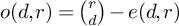 $o(d,r) = \binom {r}{d} - e(d,r)$
. The numbers
$o(d,r) = \binom {r}{d} - e(d,r)$
. The numbers
 $e(d,r)$
and
$e(d,r)$
and
 $o(d,r)$
satisfy the following recurrence relations:
$o(d,r)$
satisfy the following recurrence relations:
-
1. if d is even, then
$$ \begin{align*} e(d-1,r-1) + e(d,r-1) & = e(d,r) \\ o(d-1,r-1) + o(d,r-1) & = o(d,r); \text{ and} \end{align*} $$
-
2. if d is odd, then
$$ \begin{align*} e(d-1,r-1) + o(d,r-1) & = e(d,r) \\ o(d-1,r-1) + e(d,r-1) & = o(d,r). \end{align*} $$


Closed formulae for the entries of Losanitsch’s triangle and its complement in Pascal’s triangle are given by
 $$ \begin{align*} e(d,r) & = \frac{1}{2}\left(\binom{r}{d} + \mathbf{1}_A(r,d)\binom{\lfloor r/2 \rfloor}{\lfloor d/2 \rfloor}\right) \\ o(d,r) & = \frac{1}{2}\left(\binom{r}{d} - \mathbf{1}_A(r,d)\binom{\lfloor r/2 \rfloor}{\lfloor d/2 \rfloor}\right), \end{align*} $$
where
 $A \subseteq \mathbb {N} \times \mathbb {N}$
is the subset of pairs
$A \subseteq \mathbb {N} \times \mathbb {N}$
is the subset of pairs
 $(r,d)$
with either r odd or r and d both even, and
$(r,d)$
with either r odd or r and d both even, and
 $\mathbf {1}_A$
is its indicator function. The closed formula is proved by induction from the recurrence relations.
$\mathbf {1}_A$
is its indicator function. The closed formula is proved by induction from the recurrence relations.
Theorem 5.1. The compactly supported
 $\mathbb {A}^1$
-Euler characteristic of the Grassmannian
$\mathbb {A}^1$
-Euler characteristic of the Grassmannian
 $\operatorname {\mathrm {Gr}}(d,r)$
is
$\operatorname {\mathrm {Gr}}(d,r)$
is
 $$ \begin{align} \chi_c^{\mathrm{mot}}(\operatorname{\mathrm{Gr}}(d,r)) = e(d,r) \langle 1 \rangle + o(d,r) \langle -1 \rangle, \end{align} $$
with
 $e(d,r)$
and
$e(d,r)$
and
 $o(d,r)$
as above.
$o(d,r)$
as above.
Proof. The closed immersion
 $\operatorname {\mathrm {Gr}}(d-1,r-1) \rightarrow \operatorname {\mathrm {Gr}}(d,r)$
, yields the recursive formula
$\operatorname {\mathrm {Gr}}(d-1,r-1) \rightarrow \operatorname {\mathrm {Gr}}(d,r)$
, yields the recursive formula
 $$ \begin{align*} \chi_c^{\mathrm{mot}}(\operatorname{\mathrm{Gr}}(d,r)) = \chi_c^{\mathrm{mot}}(\operatorname{\mathrm{Gr}}(d-1,r-1)) + \langle (-1)^d \rangle \chi_c^{\mathrm{mot}}(\operatorname{\mathrm{Gr}}(d,r-1)), \end{align*} $$
If d is even, then
 $$ \begin{align*} \chi_c^{\mathrm{mot}}(\operatorname{\mathrm{Gr}}(d,r)) & = \chi_c^{\mathrm{mot}}(\operatorname{\mathrm{Gr}}(d-1,r-1)) + \chi_c^{\mathrm{mot}}(\operatorname{\mathrm{Gr}}(d,r-1)), \\ & = (e(d-1,r-1) + e(d,r-1))\langle 1 \rangle \\ & \quad + (o(d-1,r-1) + o(d,r-1))\langle -1 \rangle. \end{align*} $$
If d is odd, then
 $$ \begin{align*} \chi_c^{\mathrm{mot}}(\operatorname{\mathrm{Gr}}(d,r)) & = \chi_c^{\mathrm{mot}}(\operatorname{\mathrm{Gr}}(d-1,r-1)) + \langle -1 \rangle \chi_c^{\mathrm{mot}}(\operatorname{\mathrm{Gr}}(d,r-1)), \\ & = (e(d-1,r-1) + o(d,r-1))\langle 1 \rangle \\ & \quad + (o(d-1,r-1) + e(d,r-1))\langle -1 \rangle. \end{align*} $$
The result follows from the recurrence relations for
 $e(d,r)$
and
$e(d,r)$
and
 $o(d,r)$
above.
$o(d,r)$
above.
Theorem 5.2. The compactly supported
 $\mathbb {A}^1$
-Euler characteristic of the n-th symmetric power of the Grassmannian
$\mathbb {A}^1$
-Euler characteristic of the n-th symmetric power of the Grassmannian
 $\operatorname {\mathrm {Gr}}(d,r)$
is given by
$\operatorname {\mathrm {Gr}}(d,r)$
is given by
 $$ \begin{align*} \chi_c^{\mathrm{mot}}(\operatorname{\mathrm{Gr}}(d,r)^{(n)}) = \sum_{i=0}^{n} \binom{e(d,r) + i - 1}{i}\binom{o(d,r) + n - i - 1}{n - i} \langle (-1)^{n-i} \rangle. \end{align*} $$
Proof. Since Grassmannians are linear, they are
 $\mathrm {K}_0$
-étale linear, so apply Theorem 4.8 to Theorem 5.1 to obtain
$\mathrm {K}_0$
-étale linear, so apply Theorem 4.8 to Theorem 5.1 to obtain
 $$ \begin{align*} \chi_c^{\mathrm{mot}}(\operatorname{\mathrm{Gr}}(d,r)^{(n)}) & = a_n(\chi_c^{\mathrm{mot}}(\operatorname{\mathrm{Gr}}(d,r))) \\ & = a_n \left( e(d,r) \langle 1 \rangle + o(d,r) \langle -1 \rangle \right) \\ & = \sum_{i=0}^{n} a_{n-i}\left( e(d,r) \langle 1 \rangle \right) a_{i}\left( o(d,r) \langle -1 \rangle \right) \\ & = \sum_{i=0}^{n} \binom{e(d,r) + n - i - 1}{n - i}\binom{o(d,r) + i - 1}{i} \langle (-1)^{i} \rangle, \end{align*} $$
where we use Lemma 2.9 in order to go to the last line.
Corollary 5.3. The generating series for the compactly supported
 $\mathbb {A}^1$
-Euler characteristic of symmetric powers of
$\mathbb {A}^1$
-Euler characteristic of symmetric powers of
 $\operatorname {\mathrm {Gr}}(d,r)$
is given by
$\operatorname {\mathrm {Gr}}(d,r)$
is given by
 $$ \begin{align*} \sum_{n=0}^\infty \chi_c^{\mathrm{mot}}(\mathrm{Gr}(d,r)^{(n)})t^n = (1-t)^{-e(d,r)} (1- \langle -1 \rangle t)^{-o(d,r)} \in \operatorname{\mathrm{GW}}(k)[[t]]. \end{align*} $$
Proof. This follows immediately from Theorem 5.2 by taking the Taylor series expansion of the terms
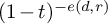 $(1-t)^{-e(d,r)}$
and
$(1-t)^{-e(d,r)}$
and
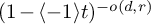 $(1- \langle -1 \rangle t)^{-o(d,r)}$
.
$(1- \langle -1 \rangle t)^{-o(d,r)}$
.
Corollary 5.4. Take
 $k=\mathbb {R}$
to be our base field, and consider
$k=\mathbb {R}$
to be our base field, and consider
 $\mathrm {Gr}(d,r)/k$
. For T a CW-complex, write
$\mathrm {Gr}(d,r)/k$
. For T a CW-complex, write
 $e_c(T)$
to mean the compactly supported Euler characteristic of T. Then compactly supported Euler characteristics of the complex and real points of
$e_c(T)$
to mean the compactly supported Euler characteristic of T. Then compactly supported Euler characteristics of the complex and real points of
 $\mathrm {Gr}(d,r)^{(n)}$
respectively fit into the following power series in
$\mathrm {Gr}(d,r)^{(n)}$
respectively fit into the following power series in
 $\mathbb {Z}[[t]]$
 $$ \begin{align*} \sum_{n=0}^\infty e_c(\mathrm{Gr}(d,r)^{(n)})(\mathbb{C}))^n &= (1-t)^{n \choose d},\\ \sum_{n=0}^\infty e(\mathrm{Gr}(d,r)^{(n)}(\mathbb{R}))t^n &= (1-t)^{-e(d,r)} (1+t)^{-o(d,r)}. \end{align*} $$
Proof. The first result follows by applying the homomorphism
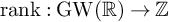 $\mathrm {rank}: \operatorname {\mathrm {GW}}(\mathbb {R}) \to \mathbb {Z}$
and using [Reference LevineLev20, Remark 2.3.1] to see that
$\mathrm {rank}: \operatorname {\mathrm {GW}}(\mathbb {R}) \to \mathbb {Z}$
and using [Reference LevineLev20, Remark 2.3.1] to see that
 $\mathrm {rank}(\chi _c^{\mathrm {mot}}(X)) = e(X(\mathbb {C}))$
(see [Reference Pajwani and PálPPa, Theorem 2.14] for the extension of this result to the compactly supported case). The result about the real points follows by instead applying
$\mathrm {rank}(\chi _c^{\mathrm {mot}}(X)) = e(X(\mathbb {C}))$
(see [Reference Pajwani and PálPPa, Theorem 2.14] for the extension of this result to the compactly supported case). The result about the real points follows by instead applying
 $\mathrm {sign}: \operatorname {\mathrm {GW}}(\mathbb {R}) \to \mathbb {Z}$
and using [Reference LevineLev20, Remark 2.3.1] which shows that
$\mathrm {sign}: \operatorname {\mathrm {GW}}(\mathbb {R}) \to \mathbb {Z}$
and using [Reference LevineLev20, Remark 2.3.1] which shows that
 $\mathrm {sign}(\chi _c^{\mathrm {mot}}(X)) = e_c(X(\mathbb {R}))$
(see also [Reference Pajwani and PálPPa, Theorem 2.20] for the extension of this result to the compactly supported case).
$\mathrm {sign}(\chi _c^{\mathrm {mot}}(X)) = e_c(X(\mathbb {R}))$
(see also [Reference Pajwani and PálPPa, Theorem 2.20] for the extension of this result to the compactly supported case).
5.2 del Pezzo surfaces
In this subsection, we use the techniques from Section 4 to show a large class of del Pezzo surfaces are symmetrisable. These are a class of surfaces of arithmetic interest, famous for the fact that over the complex numbers they contain a finite number of exceptional curves lying on them. This number is well known from enumerative geometry, for example: smooth projective cubic surfaces are del Pezzo surfaces of degree
 $3$
, the exceptional curves are precisely the lines on the surface, and it is well known that exactly
$3$
, the exceptional curves are precisely the lines on the surface, and it is well known that exactly
 $27$
lines lie on the surface over the complex numbers. Quadratically enriched counts of the number of exceptional curves on del Pezzo surfaces were achieved by Kass-Wickelgren [Reference Leo Kass and WickelgrenKW21, Theorem 2] in degree
$27$
lines lie on the surface over the complex numbers. Quadratically enriched counts of the number of exceptional curves on del Pezzo surfaces were achieved by Kass-Wickelgren [Reference Leo Kass and WickelgrenKW21, Theorem 2] in degree
 $3$
, by Darwin [Reference DarwinDar22, Theorem 1.2] in degree
$3$
, by Darwin [Reference DarwinDar22, Theorem 1.2] in degree
 $4$
, and these were generalised to the degree
$4$
, and these were generalised to the degree
 $\geq 3$
case in [Reference Leo Kass, Levine, Solomon and WickelgrenKLSW23b] and [Reference Leo Kass, Levine, Solomon and WickelgrenKLSW23a] by Kass, Levine, Solomon and Wickelgren.
$\geq 3$
case in [Reference Leo Kass, Levine, Solomon and WickelgrenKLSW23b] and [Reference Leo Kass, Levine, Solomon and WickelgrenKLSW23a] by Kass, Levine, Solomon and Wickelgren.
Definition 5.1. A del Pezzo surface is a smooth projective variety of dimension
 $2$
whose anticanonical bundle is ample. The degree of a del Pezzo surface is the self intersection number of the anticanonical class. An exceptional curve on a del Pezzo surface is a curve with self intersection number
$2$
whose anticanonical bundle is ample. The degree of a del Pezzo surface is the self intersection number of the anticanonical class. An exceptional curve on a del Pezzo surface is a curve with self intersection number
 $-1$
.
$-1$
.
The following classification of del Pezzo surfaces is due to Manin over algebraically closed fields, which we can weaken to separably closed fields by a result of Coombes.
Theorem 5.5 (Theorem 24.4 of [Reference ManinMan86], Theorem 1 of [Reference CoombesCoo88])
Let
 $\overline {k}$
be a separably closed field and let
$\overline {k}$
be a separably closed field and let
 $X/\overline {k}$
be a del Pezzo surface of degree d. Then
$X/\overline {k}$
be a del Pezzo surface of degree d. Then
 $1 \leq d \leq 9$
and either:
$1 \leq d \leq 9$
and either:
-
1.
$X \cong \mathbb {P}^1 \times \mathbb {P}^1$
and
$d=8$
. -
2. X is isomorphic to the blow up of
$\mathbb {P}^2$
at
$9-d$
points in general position.


While del Pezzo surfaces can be arithmetically very complicated, once we base change to the separable closure of our field, they are linear, so we would expect large classes of del Pezzo surfaces to be symmetrisable.
Theorem 5.6. Let
 $X/k$
be a del Pezzo surface of degree
$X/k$
be a del Pezzo surface of degree
 $\geq 5$
such that
$\geq 5$
such that
 $X(k) \neq \emptyset $
. Then X is symmetrisable.
$X(k) \neq \emptyset $
. Then X is symmetrisable.
Proof. This proceeds by checking on a case by case basis that the conditions we have already established for X to be symmetrisable for such del Pezzo surfaces. We appeal to [Reference PoonenPoo17, Section 9.4], and we sketch the main results here.
Suppose X is a del Pezzo surface of degree
 $9$
. Then X is an even dimensional Severi Brauer variety, and since
$9$
. Then X is an even dimensional Severi Brauer variety, and since
 $X(k) \neq \emptyset $
, we see
$X(k) \neq \emptyset $
, we see
 $X \cong \mathbb {P}^2$
, so X is
$X \cong \mathbb {P}^2$
, so X is
 $\mathrm {K}_0$
-étale linear and so symmetrisable by Theorem 4.8.
$\mathrm {K}_0$
-étale linear and so symmetrisable by Theorem 4.8.
Suppose X is degree
 $8$
. By [Reference PoonenPoo17, Proposition 9.4.12], we see X is either
$8$
. By [Reference PoonenPoo17, Proposition 9.4.12], we see X is either
 $\mathrm {Res}_{L/k}(C)$
where
$\mathrm {Res}_{L/k}(C)$
where
 $L/k$
is a quadratic étale algebra and C is a conic, or
$L/k$
is a quadratic étale algebra and C is a conic, or
 $\mathbb {P}^2$
blown up at a point. In the latter case the result holds by Corollary 4.11. Suppose X is the Weil restriction of a conic. Then
$\mathbb {P}^2$
blown up at a point. In the latter case the result holds by Corollary 4.11. Suppose X is the Weil restriction of a conic. Then
 $X(k) \neq \emptyset $
implies that
$X(k) \neq \emptyset $
implies that
 $C(L) \neq \emptyset $
so
$C(L) \neq \emptyset $
so
 $C_L \cong \mathbb {P}^1_L$
. Therefore
$C_L \cong \mathbb {P}^1_L$
. Therefore
 $\mathrm {Res}_{L/k}(C) = \mathbb {P}^1 \times \mathbb {P}^1$
, which is symmetrisable by Theorem 4.8.
$\mathrm {Res}_{L/k}(C) = \mathbb {P}^1 \times \mathbb {P}^1$
, which is symmetrisable by Theorem 4.8.
Suppose X is degree
 $7$
. Then by [Reference PoonenPoo17, Proposition 9.4.17], X is isomorphic to the blow up of
$7$
. Then by [Reference PoonenPoo17, Proposition 9.4.17], X is isomorphic to the blow up of
 $\mathbb {P}^2$
at a closed subscheme isomorphic to a finite étale algebra of degree
$\mathbb {P}^2$
at a closed subscheme isomorphic to a finite étale algebra of degree
 $2$
, so the result holds by Corollary 4.11. Note that this Proposition does not require X to have a k point.
$2$
, so the result holds by Corollary 4.11. Note that this Proposition does not require X to have a k point.
Suppose X has degree
 $5$
. Then by [Reference PoonenPoo17, Proposition 9.4.20], if there exists a k-point of X lying on none of the exceptional curves in X, we may obtain X through blowing up and and blowing down
$5$
. Then by [Reference PoonenPoo17, Proposition 9.4.20], if there exists a k-point of X lying on none of the exceptional curves in X, we may obtain X through blowing up and and blowing down
 $\mathbb {P}^2$
. By [Reference PoonenPoo17, Theorem 9.4.29], this is always the case unless
$\mathbb {P}^2$
. By [Reference PoonenPoo17, Theorem 9.4.29], this is always the case unless
 $k=\mathbb {F}_2, \mathbb {F}_4$
or
$k=\mathbb {F}_2, \mathbb {F}_4$
or
 $\mathbb {F}_3$
. Therefore X is symmetrisable under our assumptions on k by Corollary 4.11 unless
$\mathbb {F}_3$
. Therefore X is symmetrisable under our assumptions on k by Corollary 4.11 unless
 $k=\mathbb {F}_3$
, since we are assuming k has characteristic not
$k=\mathbb {F}_3$
, since we are assuming k has characteristic not
 $2$
. It only remains to tackle the case that
$2$
. It only remains to tackle the case that
 $k=\mathbb {F}_3$
and all k points of X lie on the exceptional curves in X. In this case X is isomorphic to
$k=\mathbb {F}_3$
and all k points of X lie on the exceptional curves in X. In this case X is isomorphic to
 $\mathbb {P}^2_k$
blown up at
$\mathbb {P}^2_k$
blown up at
 $4$
points by [Reference PoonenPoo17, Theorem 9.4.29], which gives the result by Corollary 4.11.
$4$
points by [Reference PoonenPoo17, Theorem 9.4.29], which gives the result by Corollary 4.11.
Suppose X is degree
 $6$
, and let
$6$
, and let
 $x \in X(k)$
. Using [Reference PoonenPoo17, Proposition 9.4.20], if x lies on exactly one exceptional curve
$x \in X(k)$
. Using [Reference PoonenPoo17, Proposition 9.4.20], if x lies on exactly one exceptional curve
 $E_i$
, then we may blow down X to obtain a del Pezzo surface of degree
$E_i$
, then we may blow down X to obtain a del Pezzo surface of degree
 $7$
. Therefore, X is symmetrisable by the degree
$7$
. Therefore, X is symmetrisable by the degree
 $7$
case and Corollary 4.11. If x lies on an intersection of exceptional curves, then we may blow down two other exceptional curves to obtain a del Pezzo surface of degree
$7$
case and Corollary 4.11. If x lies on an intersection of exceptional curves, then we may blow down two other exceptional curves to obtain a del Pezzo surface of degree
 $8$
, so X is symmetrisable by Corollary 4.11 and the degree
$8$
, so X is symmetrisable by Corollary 4.11 and the degree
 $8$
case. Finally, if x does not lie on any exceptional curves, we blow up X at x to obtain a del Pezzo surface of degree
$8$
case. Finally, if x does not lie on any exceptional curves, we blow up X at x to obtain a del Pezzo surface of degree
 $5$
, so X is symmetrisable by the degree
$5$
, so X is symmetrisable by the degree
 $5$
case and Corollary 4.11.
$5$
case and Corollary 4.11.
Remark 5.7. Even without the assumption that
 $X(k) \neq \emptyset $
, if X is a del Pezzo surface of degree
$X(k) \neq \emptyset $
, if X is a del Pezzo surface of degree
 $5$
or
$5$
or
 $7$
, then the above work and [Reference PoonenPoo17, Theorem 9.4.29] tells us that X is birational to
$7$
, then the above work and [Reference PoonenPoo17, Theorem 9.4.29] tells us that X is birational to
 $\mathbb {P}^2$
. If k is infinite, the k points of
$\mathbb {P}^2$
. If k is infinite, the k points of
 $\mathbb {P}^2$
are Zariski dense, and so we automatically have that
$\mathbb {P}^2$
are Zariski dense, and so we automatically have that
 $X(k) \neq \emptyset $
. If X is a del Pezzo surface of degree
$X(k) \neq \emptyset $
. If X is a del Pezzo surface of degree
 $9$
, then it is a Severi–Brauer surface. We also see del Pezzo surfaces of degree
$9$
, then it is a Severi–Brauer surface. We also see del Pezzo surfaces of degree
 $6$
which are given by blow ups of Severi–Brauer surfaces at a point are also symmetrisable by Corollary 4.11, so the above also holds for certain del Pezzo surfaces with no k-point.
$6$
which are given by blow ups of Severi–Brauer surfaces at a point are also symmetrisable by Corollary 4.11, so the above also holds for certain del Pezzo surfaces with no k-point.
The reason we restrict to the degree
 $\geq 5$
case above is that for del Pezzo surfaces X of degree
$\geq 5$
case above is that for del Pezzo surfaces X of degree
 $\geq 5$
such that
$\geq 5$
such that
 $X(k) \neq \emptyset $
, we have that X is birational to
$X(k) \neq \emptyset $
, we have that X is birational to
 $\mathbb {P}^2$
, by the steps taken in the proof above. We can therefore obtain all such del Pezzo surfaces by iterating blow-ups and blow-downs, which do not change symmetrisability by Corollary 4.11.
$\mathbb {P}^2$
, by the steps taken in the proof above. We can therefore obtain all such del Pezzo surfaces by iterating blow-ups and blow-downs, which do not change symmetrisability by Corollary 4.11.
When X has degree
 $\leq 4$
, this is no longer true: there exist del Pezzo surfaces of degree
$\leq 4$
, this is no longer true: there exist del Pezzo surfaces of degree
 $\leq 4$
which are not birational to
$\leq 4$
which are not birational to
 $\mathbb {P}^2$
. However we can obtain similar results using Corollary 4.11 for any del Pezzo surface of degree
$\mathbb {P}^2$
. However we can obtain similar results using Corollary 4.11 for any del Pezzo surface of degree
 $\leq 4$
which can be obtained via iterating blow ups and blow downs of
$\leq 4$
which can be obtained via iterating blow ups and blow downs of
 $\mathbb {P}^2$
.
$\mathbb {P}^2$
.
We can also use our results to show the following.
Theorem 5.8. Let
 $X/k$
be a diagonal cubic surface. Then X is symmetrisable.
$X/k$
be a diagonal cubic surface. Then X is symmetrisable.
Proof. We first claim that the diagonal cubic surface Y defined by the equation
 $$ \begin{align*}Y: x^3 + y^3 + z^3 = t^3 \subseteq \mathbb{P}^3_{[x:y:z:t]} \end{align*} $$
is
 $\mathrm {K}_0$
-étale linear. Note that Y contains
$\mathrm {K}_0$
-étale linear. Note that Y contains
 $2$
skew lines defined over k: namely, the lines
$2$
skew lines defined over k: namely, the lines
 $L_1: \{ x=t, y=-z\}$
and
$L_1: \{ x=t, y=-z\}$
and
 $L_2: \{x=-t, y=z\}$
. Therefore we may blow Y down at these
$L_2: \{x=-t, y=z\}$
. Therefore we may blow Y down at these
 $2$
lines to obtain a del Pezzo surface of degree
$2$
lines to obtain a del Pezzo surface of degree
 $5$
. This del Pezzo surface will have a k-point, since the skew lines are defined over k, so is symmetrisable by Theorem 5.6, and therefore Y is symmetrisable by Corollary 4.11.
$5$
. This del Pezzo surface will have a k-point, since the skew lines are defined over k, so is symmetrisable by Theorem 5.6, and therefore Y is symmetrisable by Corollary 4.11.
For the general case, a diagonal cubic surface X is defined by an equation
 $$ \begin{align*}X: a_1x^3 + a_2y^3 + a_3z^3 = t^3 \subseteq \mathbb{P}^3_{[x:y:z:t]}, \end{align*} $$
for some
 $a_1, a_2, a_3 \in k^\times $
. Therefore, X and Y become isomorphic once we base change to the field
$a_1, a_2, a_3 \in k^\times $
. Therefore, X and Y become isomorphic once we base change to the field
 $L := k(\sqrt [3]{a_1}, \sqrt [3]{a_2}, \sqrt [3]{a_3})$
. Note that
$L := k(\sqrt [3]{a_1}, \sqrt [3]{a_2}, \sqrt [3]{a_3})$
. Note that
 $[L:k] = 3^i$
where
$[L:k] = 3^i$
where
 $i \in \{0,1,2,3\}$
. In particular, we can apply Theorem 4.14 to obtain the result.
$i \in \{0,1,2,3\}$
. In particular, we can apply Theorem 4.14 to obtain the result.
To demonstrate the computational utility of Theorem 4.8, we give an explicit computation of the compactly supported
 $\mathbb {A}^1$
-Euler characteristic of the third symmetric power of a class of cubic surfaces. Let
$\mathbb {A}^1$
-Euler characteristic of the third symmetric power of a class of cubic surfaces. Let
 $\alpha , \beta , \gamma \in k^\times $
be non squares. Let Y be a closed embedding of
$\alpha , \beta , \gamma \in k^\times $
be non squares. Let Y be a closed embedding of
 $\operatorname {\mathrm {Spec}}(k(\sqrt {\alpha })) \amalg \operatorname {\mathrm {Spec}}(k(\sqrt {\beta })) \amalg \operatorname {\mathrm {Spec}}(k(\sqrt {\gamma }))$
into
$\operatorname {\mathrm {Spec}}(k(\sqrt {\alpha })) \amalg \operatorname {\mathrm {Spec}}(k(\sqrt {\beta })) \amalg \operatorname {\mathrm {Spec}}(k(\sqrt {\gamma }))$
into
 $\mathbb {P}^2$
such that the six points of
$\mathbb {P}^2$
such that the six points of
 $Y_{\overline {k}}(\overline {k})$
lie in general position in
$Y_{\overline {k}}(\overline {k})$
lie in general position in
 $\mathbb {P}_{\overline {k}}^2(\overline {k})$
. Let
$\mathbb {P}_{\overline {k}}^2(\overline {k})$
. Let
 $X := \mathrm {Bl}_Y(\mathbb {P}^2)$
, so
$X := \mathrm {Bl}_Y(\mathbb {P}^2)$
, so
 $X/k$
is a smooth cubic surface which is symmetrisable by Corollary 4.11.
$X/k$
is a smooth cubic surface which is symmetrisable by Corollary 4.11.
Proposition 5.9. We see that
 $$ \begin{align*}\chi_c^{\mathrm{mot}}(X) = 2 \langle 1 \rangle + 4 \langle -1 \rangle + \langle -\alpha \rangle + \langle - \beta \rangle + \langle -\gamma \rangle.\end{align*} $$
Proof. By the blow up formula for
 $\chi _c^{\mathrm {mot}}$
, we see that
$\chi _c^{\mathrm {mot}}$
, we see that
 $$ \begin{align*}\chi_c^{\mathrm{mot}}(X) = \chi_c^{\mathrm{mot}}(\mathbb{P}^2) + \chi_c^{\mathrm{mot}}(E) - \chi_c^{\mathrm{mot}}(Y), \end{align*} $$
where E is the exceptional divisor of the blow up. The exceptional divisor is a
 $\mathbb {P}^1$
bundle over Y, so
$\mathbb {P}^1$
bundle over Y, so
 $\chi _c^{\mathrm {mot}}(E) = \chi _c^{\mathrm {mot}}(\mathbb {P}^1) \cdot \chi _c^{\mathrm {mot}}(Y)$
. Note that
$\chi _c^{\mathrm {mot}}(E) = \chi _c^{\mathrm {mot}}(\mathbb {P}^1) \cdot \chi _c^{\mathrm {mot}}(Y)$
. Note that
 $\chi _c^{\mathrm {mot}}(\mathbb {P}^1) = \mathbb {H}$
, so
$\chi _c^{\mathrm {mot}}(\mathbb {P}^1) = \mathbb {H}$
, so
 $\chi _c^{\mathrm {mot}}(E) - \chi _c^{\mathrm {mot}}(Y) = \langle -1 \rangle \cdot \chi _c^{\mathrm {mot}}(Y)$
. By [Reference HoyoisHoy14, Proposition 5.2], we see that if
$\chi _c^{\mathrm {mot}}(E) - \chi _c^{\mathrm {mot}}(Y) = \langle -1 \rangle \cdot \chi _c^{\mathrm {mot}}(Y)$
. By [Reference HoyoisHoy14, Proposition 5.2], we see that if
 $L/k$
is a finite field extension, then
$L/k$
is a finite field extension, then
 $\chi _c^{\mathrm {mot}}(\operatorname {\mathrm {Spec}}(L)) = [\mathrm {Tr}_{L/k}]$
, where
$\chi _c^{\mathrm {mot}}(\operatorname {\mathrm {Spec}}(L)) = [\mathrm {Tr}_{L/k}]$
, where
 $[\mathrm {Tr}_{L/k}]$
is the trace form on L. If
$[\mathrm {Tr}_{L/k}]$
is the trace form on L. If
 $L = k(\sqrt {\alpha })$
, then computing the trace form in the basis
$L = k(\sqrt {\alpha })$
, then computing the trace form in the basis
 $1, \sqrt {\alpha }$
gives
$1, \sqrt {\alpha }$
gives
 $\chi _c^{\mathrm {mot}}(\operatorname {\mathrm {Spec}}(L)) = \langle 2 \rangle + \langle 2 \alpha \rangle $
. Additivity of
$\chi _c^{\mathrm {mot}}(\operatorname {\mathrm {Spec}}(L)) = \langle 2 \rangle + \langle 2 \alpha \rangle $
. Additivity of
 $\chi _c^{\mathrm {mot}}$
implies
$\chi _c^{\mathrm {mot}}$
implies
 $$ \begin{align*}\chi_c^{\mathrm{mot}}(Y) = 3 \langle 2 \rangle + \langle 2\alpha \rangle + \langle 2\beta \rangle + \langle 2\gamma \rangle = 2\langle 1 \rangle + \langle 2 \rangle + \langle 2\alpha \rangle + \langle 2\beta \rangle + \langle 2\gamma \rangle \end{align*} $$
Finally,
 $\chi _c^{\mathrm {mot}}(\mathbb {P}^2) = 2\langle 1\rangle +\langle -1 \rangle $
. Put together, this gives
$\chi _c^{\mathrm {mot}}(\mathbb {P}^2) = 2\langle 1\rangle +\langle -1 \rangle $
. Put together, this gives
 $$ \begin{align*}\chi_c^{\mathrm{mot}}(X) = 2 \mathbb{H} + \langle -1 \rangle + \langle -2 \rangle + \langle -2\alpha \rangle + \langle - 2\beta \rangle + \langle -2\gamma \rangle.\\[-33pt] \end{align*} $$
Corollary 5.10. For
 $X/k$
our cubic surface as above, the compactly supported
$X/k$
our cubic surface as above, the compactly supported
 $\mathbb {A}^1$
- Euler characteristic of its third symmetric power is given by
$\mathbb {A}^1$
- Euler characteristic of its third symmetric power is given by
 $$ \begin{align*} \chi_c^{\mathrm{mot}}(X^{(3)}) &= 60\mathbb{H} + 11 \langle -1 \rangle + 3\langle -2 \rangle \\ &\quad + 7\left( \langle -2\alpha \rangle + \langle -2\beta \rangle + \langle -2\gamma \rangle \right) + \left(\langle -\alpha \rangle + \langle -\beta \rangle + \langle -\gamma \rangle \right) \\&\quad + \left( \langle 1 \rangle + \langle 2 \rangle \right)\left( \langle \alpha\beta \rangle + \langle \alpha\gamma \rangle + \langle \beta\gamma \rangle \right)\\&\quad + \langle -2\alpha\beta\gamma \rangle + t_{\alpha \beta} + t_{\beta \gamma} + t_{\alpha \gamma} \end{align*} $$
Proof. Since X is symmetrisable, we see that
 $\chi _c^{\mathrm {mot}}(X^{(3)}) = a_3(\chi _c^{\mathrm {mot}}(X))$
. We may compute
$\chi _c^{\mathrm {mot}}(X^{(3)}) = a_3(\chi _c^{\mathrm {mot}}(X))$
. We may compute
 $a_3(\chi _c^{\mathrm {mot}}(X))$
, using the additive formula for the
$a_3(\chi _c^{\mathrm {mot}}(X))$
, using the additive formula for the
 $a_n$
s, to obtain
$a_n$
s, to obtain
 $$ \begin{align*} \chi_c^{\mathrm{mot}}(X^{(3)}) &= a_3( 2 \langle 1 \rangle + 3 \langle -1 \rangle + \langle -2 \rangle) \\ &\quad + a_2( 2 \langle 1 \rangle + 3 \langle -1 \rangle + \langle -2 \rangle) \cdot \left( \langle -2\alpha \rangle + \langle -2\beta \rangle + \langle -2\gamma \rangle \right) \\ &\quad + ( 2 \langle 1 \rangle + 3 \langle -1 \rangle + \langle -2 \rangle) \cdot a_2(\langle -2\alpha \rangle + \langle -2\beta \rangle + \langle -2\gamma \rangle) \\ &\quad + a_3(\langle -2\alpha \rangle + \langle -2\beta \rangle + \langle -2\gamma \rangle). \end{align*} $$
Write
 $\phi = \langle -2\alpha \rangle + \langle -2\beta \rangle + \langle -2\gamma \rangle $
to ease notation. Standard computations utilising [Reference Pajwani and PálPP25, Lemmas 3.20 and 3.21] give us
$\phi = \langle -2\alpha \rangle + \langle -2\beta \rangle + \langle -2\gamma \rangle $
to ease notation. Standard computations utilising [Reference Pajwani and PálPP25, Lemmas 3.20 and 3.21] give us
 $$ \begin{align*} a_3( 2\mathbb{H} + \langle -1 \rangle + \langle -2 \rangle) &= 24\mathbb{H} + 8 \langle -1 \rangle \\ a_2( 2\mathbb{H} + \langle -1 \rangle + \langle -2 \rangle)\phi &= 24 \mathbb{H} + +4 \phi + \langle 2\rangle \phi \\ ( 2 \langle 1 \rangle + 3 \langle -1 \rangle + \langle -2 \rangle) \cdot a_2(\phi) &= 12\mathbb{H} + (\langle -1 \rangle + \langle -2 \rangle) \left( 3\langle 1 \rangle + \langle -\alpha \beta \rangle + \langle - \beta \gamma \rangle + \langle - \alpha\gamma \rangle\right) \\ a_3(\phi) &= 3\phi + \langle - 2\alpha \beta \gamma \rangle + t_{\alpha \beta} + t_{\beta\gamma} + t_{\alpha \gamma}. \end{align*} $$
Compiling these terms and substituting our value back for
 $\phi $
gives
$\phi $
gives
 $$ \begin{align*} \chi_c^{\mathrm{mot}}(X^{(3)}) &= 60\mathbb{H} + 11 \langle -1 \rangle + 3\langle -2 \rangle \\ &\quad + 7\left( \langle -2\alpha \rangle + \langle -2\beta \rangle + \langle -2\gamma \rangle \right) + \left(\langle -\alpha \rangle + \langle -\beta \rangle + \langle -\gamma \rangle \right) \\&\quad + \left( \langle 1 \rangle + \langle 2 \rangle \right)\left( \langle \alpha\beta \rangle + \langle \alpha\gamma \rangle + \langle \beta\gamma \rangle \right)\\&\quad + \langle -2\alpha\beta\gamma \rangle + t_{\alpha \beta} + t_{\beta \gamma} + t_{\alpha \gamma}.\\[-34pt] \end{align*} $$
Remark 5.11. It should be noted that Pepin-Lehalleur and Taelman have work in progress which computes
 $X^{(n)}$
for a very general class of surfaces X. Moreover, Section 8 of [Reference Bejleri and McKeanBM25] to derives a Göttsche style formula for computing the compactly supported
$X^{(n)}$
for a very general class of surfaces X. Moreover, Section 8 of [Reference Bejleri and McKeanBM25] to derives a Göttsche style formula for computing the compactly supported
 $\mathbb {A}^1$
-Euler characteristic of Hilbert schemes of points of symmetrisable surfaces. This result is of particular interest if we can show that
$\mathbb {A}^1$
-Euler characteristic of Hilbert schemes of points of symmetrisable surfaces. This result is of particular interest if we can show that
 $\mathrm {K}3$
surfaces are symmetrisable, when X is a
$\mathrm {K}3$
surfaces are symmetrisable, when X is a
 $\mathrm {K}3$
-surface, this formula would generalise [Reference Pajwani and PálPPa, Corollary 8.18]. In characteristic
$\mathrm {K}3$
-surface, this formula would generalise [Reference Pajwani and PálPPa, Corollary 8.18]. In characteristic
 $0$
we see that
$0$
we see that
 $\mathrm {K}3$
surfaces are not in general geometrically stably rational (for example: the unramified Brauer group of a variety is a stable birational invariant, and we may find examples of
$\mathrm {K}3$
surfaces are not in general geometrically stably rational (for example: the unramified Brauer group of a variety is a stable birational invariant, and we may find examples of
 $\mathrm {K}3$
surfaces whose unramified Brauer group is non-trivial). Therefore
$\mathrm {K}3$
surfaces whose unramified Brauer group is non-trivial). Therefore
 $\mathrm {K}3$
surfaces are not in general
$\mathrm {K}3$
surfaces are not in general
 $\mathrm {K}_0$
-étale linear by Theorem 3.2, and so the results of this paper do not apply to give such a formula. However, we may apply Theorem 8.7 of [Reference Bejleri and McKeanBM25], to obtain a Göttsche formula for symmetrisable surface, and in particular, the results of our paper implies that the formula in Theorem 8.7 of [Reference Bejleri and McKeanBM25] holds whenever
$\mathrm {K}_0$
-étale linear by Theorem 3.2, and so the results of this paper do not apply to give such a formula. However, we may apply Theorem 8.7 of [Reference Bejleri and McKeanBM25], to obtain a Göttsche formula for symmetrisable surface, and in particular, the results of our paper implies that the formula in Theorem 8.7 of [Reference Bejleri and McKeanBM25] holds whenever
 $X/k$
is a del Pezzo surface of degree
$X/k$
is a del Pezzo surface of degree
 $\geq 5$
with
$\geq 5$
with
 $X(k) \neq \emptyset $
.
$X(k) \neq \emptyset $
.
6 Curves of genus
$\leq 1$

In this section we show that curves of geometric genus
 $\leq 1$
are symmetrisable, but curves of geometric genus
$\leq 1$
are symmetrisable, but curves of geometric genus
 $>0$
are not
$>0$
are not
 $\mathrm {K}_0$
-étale linear in characteristic
$\mathrm {K}_0$
-étale linear in characteristic
 $0$
. Therefore, curves of genus
$0$
. Therefore, curves of genus
 $1$
give examples to show the inclusion
$1$
give examples to show the inclusion
 $\mathrm {K}_0(\mathrm {\acute {E}tLin}_k) \subseteq \mathrm {K}_0(\mathrm {Sym}_k)$
is strict.
$\mathrm {K}_0(\mathrm {\acute {E}tLin}_k) \subseteq \mathrm {K}_0(\mathrm {Sym}_k)$
is strict.
Remark 6.1. The following proposition was initially proven only in characteristic
 $0$
and before the paper [Reference Bröring and ViergeverBV25], which shows that all curves are symmetrisable, both in characteristic
$0$
and before the paper [Reference Bröring and ViergeverBV25], which shows that all curves are symmetrisable, both in characteristic
 $0$
and in characteristic
$0$
and in characteristic
 $>2$
. We keep the below argument in this paper for completeness, however, we use an argument from [Reference Bröring and ViergeverBV25] to extend our original argument to characteristic p.
$>2$
. We keep the below argument in this paper for completeness, however, we use an argument from [Reference Bröring and ViergeverBV25] to extend our original argument to characteristic p.
Proposition 6.2. Let C be a smooth projective curve, and let n be odd. Then
 $\chi _c^{\mathrm {mot}}(C^{(n)}) = a_n(\chi _c^{\mathrm {mot}}(C))$
.
$\chi _c^{\mathrm {mot}}(C^{(n)}) = a_n(\chi _c^{\mathrm {mot}}(C))$
.
Proof. Note that
 $C^{(n)}$
is smooth projective of odd dimension, so
$C^{(n)}$
is smooth projective of odd dimension, so
 $\chi _c^{\mathrm {mot}}(C^{(n)})$
is hyperbolic by [Reference LevineLev20, Corollary 3.2]. Since the rank is invariant under base change of fields, we may assume k is algebraically closed by base changing to the algebraic closure of k.
$\chi _c^{\mathrm {mot}}(C^{(n)})$
is hyperbolic by [Reference LevineLev20, Corollary 3.2]. Since the rank is invariant under base change of fields, we may assume k is algebraically closed by base changing to the algebraic closure of k.
If
 $\mathrm {char}(k)=0$
we may argue as in the proof of [Reference Pajwani and PálPPa, Theorem 2.14] to reduce the result to the case where
$\mathrm {char}(k)=0$
we may argue as in the proof of [Reference Pajwani and PálPPa, Theorem 2.14] to reduce the result to the case where
 $k=\mathbb {C}$
, where the result holds by a result of MacDonald [Reference MacdonaldMac62a, (4.4)]. In positive characteristic, we may argue as in [Reference Bröring and ViergeverBV25, Lemma 9, Proposition 10] to reduce to the case where k has characteristic
$k=\mathbb {C}$
, where the result holds by a result of MacDonald [Reference MacdonaldMac62a, (4.4)]. In positive characteristic, we may argue as in [Reference Bröring and ViergeverBV25, Lemma 9, Proposition 10] to reduce to the case where k has characteristic
 $0$
.
$0$
.
Corollary 6.3. Smooth projective curves of genus
 $0$
are symmetrisable.
$0$
are symmetrisable.
Proof. Let C be a smooth projective curve of genus
 $0$
. By the above proposition, we only need to show
$0$
. By the above proposition, we only need to show
 $\chi _c^{\mathrm {mot}}(C^{(n)}) = a_n(\chi _c^{\mathrm {mot}}(C))$
when n is even. If
$\chi _c^{\mathrm {mot}}(C^{(n)}) = a_n(\chi _c^{\mathrm {mot}}(C))$
when n is even. If
 $C=\mathbb {P}^1$
, then C is linear, so the result follows by Theorem 4.8. Assume therefore that C is a conic with
$C=\mathbb {P}^1$
, then C is linear, so the result follows by Theorem 4.8. Assume therefore that C is a conic with
 $C(k) = \emptyset $
, so there exists a quadratic extension
$C(k) = \emptyset $
, so there exists a quadratic extension
 $L/k$
with
$L/k$
with
 $C(L) \neq \emptyset $
. In particular, we see there is a closed embedding
$C(L) \neq \emptyset $
. In particular, we see there is a closed embedding
 $\operatorname {\mathrm {Spec}}(L) \hookrightarrow C$
. We then see that
$\operatorname {\mathrm {Spec}}(L) \hookrightarrow C$
. We then see that
 $\operatorname {\mathrm {Spec}}(L)^{(n)}$
is a closed subvariety of
$\operatorname {\mathrm {Spec}}(L)^{(n)}$
is a closed subvariety of
 $C^{(n)}$
. Moreover, since
$C^{(n)}$
. Moreover, since
 $C^{(n)}$
is a k-form of
$C^{(n)}$
is a k-form of
 $\mathbb {P}^1$
, we see that
$\mathbb {P}^1$
, we see that
 $C^{(n)}$
will be given by a k-form of
$C^{(n)}$
will be given by a k-form of
 $(\mathbb {P}^1)^{(n)} = \mathbb {P}^n$
, so is also a Severi–Brauer variety. Note that
$(\mathbb {P}^1)^{(n)} = \mathbb {P}^n$
, so is also a Severi–Brauer variety. Note that
 $\operatorname {\mathrm {Spec}}(L)^{(n)}$
is given by the disjoint union of
$\operatorname {\mathrm {Spec}}(L)^{(n)}$
is given by the disjoint union of
 $\operatorname {\mathrm {Spec}}(k)$
and
$\operatorname {\mathrm {Spec}}(k)$
and
 $\frac {n}{2}$
copies of
$\frac {n}{2}$
copies of
 $\operatorname {\mathrm {Spec}}(L)$
, so in particular,
$\operatorname {\mathrm {Spec}}(L)$
, so in particular,
 $\operatorname {\mathrm {Spec}}(k)$
embeds as a closed subvariety into
$\operatorname {\mathrm {Spec}}(k)$
embeds as a closed subvariety into
 $C^{(n)}$
, so
$C^{(n)}$
, so
 $C^{(n)}(k) \neq \emptyset $
. Since
$C^{(n)}(k) \neq \emptyset $
. Since
 $C^{(n)}$
is a Severi–Brauer variety however, we see
$C^{(n)}$
is a Severi–Brauer variety however, we see
 $C^{(n)} = \mathbb {P}^n$
again by Châtelet’s Theorem ([Reference PoonenPoo17, Proposition 4.5.10]). The result is now clear.
$C^{(n)} = \mathbb {P}^n$
again by Châtelet’s Theorem ([Reference PoonenPoo17, Proposition 4.5.10]). The result is now clear.
Proposition 6.4. Let C be a smooth projective curve of genus
 $g>0$
. Suppose that
$g>0$
. Suppose that
 $n> 2g-2$
. Then
$n> 2g-2$
. Then
 $\chi _c^{\mathrm {mot}}(C^{(n)}) = 0$
.
$\chi _c^{\mathrm {mot}}(C^{(n)}) = 0$
.
Proof. Let
 $k^{p^{-\infty }}$
denote the perfect closure of k, which is the field given by adjoining all
$k^{p^{-\infty }}$
denote the perfect closure of k, which is the field given by adjoining all
 $p^n$
roots of elements in k for every n (see [Reference GreenbergGre65, 2.]). Since we are not in characteristic
$p^n$
roots of elements in k for every n (see [Reference GreenbergGre65, 2.]). Since we are not in characteristic
 $2$
, the map
$2$
, the map
 $\mathrm {GW}(k) \to \operatorname {\mathrm {GW}}(k^{perf})$
is an isomorphism, so without loss of generality, by base changing to
$\mathrm {GW}(k) \to \operatorname {\mathrm {GW}}(k^{perf})$
is an isomorphism, so without loss of generality, by base changing to
 $k^{perf}$
, we may assume our base field is perfect.
$k^{perf}$
, we may assume our base field is perfect.
As in the proof of [Reference MustaţăMus11, Theorem 7.33], define a morphism
 $C^{(n)}\to \text {Pic}^n(C)$
which is defined on points over the algebraic closure
$C^{(n)}\to \text {Pic}^n(C)$
which is defined on points over the algebraic closure
 $\bar {k}$
of k as follows. A point of
$\bar {k}$
of k as follows. A point of
 $C^{(n)}$
over
$C^{(n)}$
over
 $\bar {k}$
is a divisor D on C of degree n and we send D to
$\bar {k}$
is a divisor D on C of degree n and we send D to
 $\mathcal {O}_C(D)$
. If
$\mathcal {O}_C(D)$
. If
 $n>2g-2$
, this map makes
$n>2g-2$
, this map makes
 $C^{(n)}$
into a Zariski locally trivial bundle of degree
$C^{(n)}$
into a Zariski locally trivial bundle of degree
 $n-g$
over
$n-g$
over
 $\text {Pic}^n(C)$
whose fibre
$\text {Pic}^n(C)$
whose fibre
 $B^{n-g}$
is a Severi–Brauer variety of dimension
$B^{n-g}$
is a Severi–Brauer variety of dimension
 $n-g$
. We now find that
$n-g$
. We now find that
 $$ \begin{align*} \chi_c^{\mathrm{mot}}(C^{(n)}) &= \chi_c^{\mathrm{mot}}(B^{n-g})\chi_c^{\mathrm{mot}}(\text{Pic}^n(C)). \end{align*} $$
Since
 $\chi _c^{\mathrm {mot}}(\text {Pic}^n(C)) = 0$
by [Reference Pajwani and PálPPa, Theorem 5.29], this gives the result. The result [Reference Pajwani and PálPPa, Theorem 5.29] is stated in characteristic
$\chi _c^{\mathrm {mot}}(\text {Pic}^n(C)) = 0$
by [Reference Pajwani and PálPPa, Theorem 5.29], this gives the result. The result [Reference Pajwani and PálPPa, Theorem 5.29] is stated in characteristic
 $0$
, but an identical argument holds over perfect fields of characteristic
$0$
, but an identical argument holds over perfect fields of characteristic
 $\neq 2$
.
$\neq 2$
.
Corollary 6.5. Let C be a curve of geometric genus
 $\leq 1$
. Then C is symmetrisable.
$\leq 1$
. Then C is symmetrisable.
Proof. We first reduce to the case where C is smooth and projective. Let
 $\overline {C}$
be a compactification of C, and let
$\overline {C}$
be a compactification of C, and let
 $\tilde {C}$
be a normalisation of
$\tilde {C}$
be a normalisation of
 $\overline {C}$
, so that
$\overline {C}$
, so that
 $\tilde {C}$
is smooth and projective. Then
$\tilde {C}$
is smooth and projective. Then
 $\tilde {C}$
and C are birational and dimension
$\tilde {C}$
and C are birational and dimension
 $1$
, so the rational map
$1$
, so the rational map
 $\tilde {C} \dashrightarrow C$
allows us to realise
$\tilde {C} \dashrightarrow C$
allows us to realise
 $[\tilde {C}] - [A]= [C] - [A']$
, where
$[\tilde {C}] - [A]= [C] - [A']$
, where
 $A, A'$
are dimension
$A, A'$
are dimension
 $0$
varieties. Since
$0$
varieties. Since
 $\mathrm {K}_0(\mathrm {Sym}_k)$
is a sub-abelian group of
$\mathrm {K}_0(\mathrm {Sym}_k)$
is a sub-abelian group of
 $\mathrm {K}_0(\mathrm {Var}_k)$
and dimension
$\mathrm {K}_0(\mathrm {Var}_k)$
and dimension
 $0$
varieties are symmetrisable by [Reference Pajwani and PálPP25, Corollary 4.30],
$0$
varieties are symmetrisable by [Reference Pajwani and PálPP25, Corollary 4.30],
 $[C]$
is an element of
$[C]$
is an element of
 $\mathrm {K}_0(\mathrm {Sym}_k)$
if and only if
$\mathrm {K}_0(\mathrm {Sym}_k)$
if and only if
 $[\tilde {C}]$
is. Therefore, replacing C with
$[\tilde {C}]$
is. Therefore, replacing C with
 $\tilde {C}$
if necessary, assume C is smooth and projective.
$\tilde {C}$
if necessary, assume C is smooth and projective.
If
 $g(C)=0$
, we appeal to Corollary 6.3. If
$g(C)=0$
, we appeal to Corollary 6.3. If
 $g(C) = 1$
, Proposition 6.4 guarantees that
$g(C) = 1$
, Proposition 6.4 guarantees that
 $\chi _c^{\mathrm {mot}}(C^{(n)}) = 0$
for all
$\chi _c^{\mathrm {mot}}(C^{(n)}) = 0$
for all
 $n> 0$
. Since
$n> 0$
. Since
 $C^{(1)}=C$
, the result for
$C^{(1)}=C$
, the result for
 $n=1$
gives us
$n=1$
gives us
 $$ \begin{align*}\chi_c^{\mathrm{mot}}(C^{(n)})=0=a_n(0)=a_n(\chi_c^{\mathrm{mot}}(C)), \end{align*} $$
so
 $[C] \in \mathrm {K}_0(\mathrm {Sym}_k)$
as required.
$[C] \in \mathrm {K}_0(\mathrm {Sym}_k)$
as required.
Lemma 6.6. Let X be a geometrically connected curve of geometric genus
 $> 0$
, and suppose
$> 0$
, and suppose
 $\mathrm {char}(k)=0$
. Then X is not
$\mathrm {char}(k)=0$
. Then X is not
 $\mathrm {K}_0$
-étale linear.
$\mathrm {K}_0$
-étale linear.
Proof. As above, we may reduce to the case where k is algebraically closed and X is connected, and as in Corollary 6.5, we may reduce to the case where X is smooth and projective. Suppose X is stably rational, so it is unirational. Since X is a curve, this would imply X is rational by a result of Luroth ([Reference LürothLür75]). By the Riemann–Hurwitz formula
 $g(X)=0$
. For X not genus
$g(X)=0$
. For X not genus
 $0$
, it is not geometrically stably rational, so we can apply Theorem 3.2 to get the result.
$0$
, it is not geometrically stably rational, so we can apply Theorem 3.2 to get the result.
As mentioned in Remark 4.12, this shows that the inclusion
 $\mathrm {K}_0(\mathrm {\acute {E}tLin}_k)\subseteq \mathrm {K}_0(\mathrm {Sym}_k)$
is always strict in characteristic 0. In [Reference Bröring and ViergeverBV25, Proposition 26], it is shown that all curves are symmetrisable. Since
$\mathrm {K}_0(\mathrm {\acute {E}tLin}_k)\subseteq \mathrm {K}_0(\mathrm {Sym}_k)$
is always strict in characteristic 0. In [Reference Bröring and ViergeverBV25, Proposition 26], it is shown that all curves are symmetrisable. Since
 $\mathrm {K}_0(\mathrm {Sym}_k)$
is a module over
$\mathrm {K}_0(\mathrm {Sym}_k)$
is a module over
 $\mathrm {K}_0(\mathrm {\acute {E}tLin}_k)$
, we use this result to obtain large classes of symmetrisable varieties which are not
$\mathrm {K}_0(\mathrm {\acute {E}tLin}_k)$
, we use this result to obtain large classes of symmetrisable varieties which are not
 $\mathrm {K}_0$
-étale linear, for example, the product of a curve and any
$\mathrm {K}_0$
-étale linear, for example, the product of a curve and any
 $\mathrm {K}_0$
-étale linear variety.
$\mathrm {K}_0$
-étale linear variety.
Remark 6.7. For other invariants in motivic homotopy theory, we may obtain obstructions to nice behaviour for varieties which are not
 $\mathbb {A}^1$
-connected. For example, [Reference Leo Kass, Levine, Solomon and WickelgrenKLSW23b, Definition 2.30] introduces the notion of a global
$\mathbb {A}^1$
-connected. For example, [Reference Leo Kass, Levine, Solomon and WickelgrenKLSW23b, Definition 2.30] introduces the notion of a global
 $\mathbb {A}^1$
-degree of a morphism
$\mathbb {A}^1$
-degree of a morphism
 $f: X \to Y$
, which descends to an element of
$f: X \to Y$
, which descends to an element of
 $\operatorname {\mathrm {GW}}(k)$
only when Y is
$\operatorname {\mathrm {GW}}(k)$
only when Y is
 $\mathbb {A}^1$
-connected. Therefore, one might expect
$\mathbb {A}^1$
-connected. Therefore, one might expect
 $\mathbb {A}^1$
-connectedness to be a necessary condition for symmetrisability. However, when k is a number field, there exist smooth projective curves of genus
$\mathbb {A}^1$
-connectedness to be a necessary condition for symmetrisability. However, when k is a number field, there exist smooth projective curves of genus
 $\geq 1$
that are not
$\geq 1$
that are not
 $\mathbb {A}^1$
-connected. It is therefore not true that over a number field
$\mathbb {A}^1$
-connected. It is therefore not true that over a number field
 $\mathrm {K}_0(\mathrm {Sym}_k)$
is given by the Grothendieck group of (geometrically)-
$\mathrm {K}_0(\mathrm {Sym}_k)$
is given by the Grothendieck group of (geometrically)-
 $\mathbb {A}^1$
-connected varieties.
$\mathbb {A}^1$
-connected varieties.
Acknowledgements
This work was undertaken while the first author was funded by the Marsden grant “Rational points and Anabelian Geometry”, and he wishes to thank the University of Canterbury, New Zealand. The second author was supported by the ERC through the project QUADAG. This paper is part of a project that has received funding from the European Research Council (ERC) under the European Union’s Horizon 2020 research and innovation programme (grant agreement No. 832833).
The authors thank Marc Levine for pointing out the elegant proof of Proposition 6.4 and some errors in an earlier version of this preprint, as well as H. Uppal for useful conversations about del Pezzo surfaces. We also thank Margaret Bilu for helpful discussions on the paper [Reference Bilu, Ho, Srinivasan, Vogt and WickelgrenBHS+24], and Ambrus Pál for helpful discussions and worked examples which agree with the main theorem. We thank Louisa Bröring for helpful discussions on the positive characteristic case and for many useful comments on an earlier draft of this paper. We further thank Stefan Schreieder for proofreading an earlier draft of this paper.
Competing interests
The author declares none.


 Open access