

40.1 Introduction
Rhythm in speech emerges from the systematic alternation of stronger and weaker elements across several layers of prosodic organization. Yet, defining and quantifying speech rhythm remains challenging, with multiple competing frameworks and metrics proposed over the years. These efforts reflect the absence of consensus on how best to capture rhythmic structure in the speech signal and the need for continued refinement of analytic tools.
Deloche et al. (Reference Deloche, Bonnasse-Gahot and Gervain2024) provide a historical overview of perspectives and analytical methods for capturing rhythmic structure in speech, which we paraphrase in the next two paragraphs. Afterwards, we introduce our current objective.
Early accounts of rhythm emphasized the principle of isochrony—the idea that speech is organized into equally timed units, whether measured by syllables or by the intervals between stresses (Pike, Reference Pike1945; Abercrombie, Reference Abercrombie1967). This view motivated the familiar classification of languages into “syllable-timed” and “stress-timed” types (see also Chapters 30 in this volume). Subsequent empirical studies showed that natural speech rarely maintains equal timing across these units (Roach, Reference Roach1982; Dauer, Reference Bartelds, de Vries, Richter, Liberman and Wieling1983), leading to a rejection of strict isochrony. Even so, the term speech rhythm and the associated typology persist because alternations in prominence at multiple prosodic levels still give rise to the perception of rhythm (Langus et al., Reference Langus, Mehler and Nespor2017), which depends on physical dimensions such as intensity, duration, pitch, and vowel quality (Terken & Hermes, Reference Terken, Hermes and Horne2000). For typology and modeling alike, this broader view keeps rhythm anchored in observable timing and prominence patterns rather than in idealized equal units.
Following this paradigm shift, the field moved from searching for perfectly timed intervals to characterizing subtler regularities distributed across multiple temporal and spectral dimensions (Bertinetto, Reference Bertinetto1989; Kohler, Reference Kohler2009; Cumming & Nolan, Reference Cumming2010; Turk & Shattuck-Hufnagel, Reference Turk and Shattuck-Hufnagel2013). Dauer (Reference Bartelds, de Vries, Richter, Liberman and Wieling1983) proposed linking rhythmic classes to structural properties of languages—such as syllable complexity and the presence of vowel reduction—laying the foundation for duration-based rhythm metrics. These metrics, which quantify the variability of consonantal and vocalic intervals, offered the first large-scale quantitative evidence supporting rhythm classes (Ramus et al., Reference Ramus, Nespor and Mehler1999; Grabe & Low, Reference Grabe and Low2002; see also Chapter 30 for an overview). Despite their ability to distinguish prototypical stress-timed and syllable-timed languages, these measures are highly sensitive to changes in speech rate, style, and task, sometimes producing within-language variability greater than cross-linguistic differences (Arvaniti, Reference Arvaniti2009, Reference Arvaniti2012; Wiget et al., Reference Wiget, White and Schuppler2010). As noted by Deloche et al. (Reference Deloche, Bonnasse-Gahot and Gervain2024), these limitations underscore the need for approaches that go beyond interval statistics to reassess the acoustic basis of rhythm and to connect linguistic intuitions with stable statistical regularities in real speech.
In our own current work, we focus on how listeners acquire the rhythm of a non-native language, which has historically received less attention than studies of segmental learning. A key question we are interested in is whether having an L1 with similar rhythmic structure facilitates acquisition of an L2’s rhythm. Evidence to date suggests that shared rhythmic patterns in the L1 can support learning of the L2 rhythm, whereas a mismatch can pose persistent challenges. For instance, German learners of English often achieve a degree of durational variability similar to native British English, while French learners show lower variability even at advanced proficiency (Ordin & Polyanskaya, Reference Ordin and Polyanskaya2015). Yet, as Van Maastricht et al. (Reference Van Maastricht, Krahmer, Swerts and Prieto2019) note, such findings must be interpreted cautiously, as differences may also arise from segmental, phonotactic, or prosodic disparities between the languages being compared.
The present study seeks to extend this work by testing whether rhythm similarity facilitates acquisition both across distinct L1–L2 pairings and within the same pairing at different proficiency levels. Specifically, we analyze English rhythm acquisition by native speakers of German and French, and German rhythm acquisition by native speakers of English and French. Within the German–English pairing, we further examine how English and French are acquired by native German speakers. A key methodological advance of this study is that L2 proficiency is indexed not merely by self-report or exposure but by the degree of acoustic distance between L1 and L2, following Bartelds et al. (Reference Bartelds, de Vries, Richter, Liberman and Wieling2021, Reference Bartelds, de Vries and Sanal2022). Crucially, rather than focusing exclusively on the variability of consonantal and vocalic intervals, we assess temporal regularities by measuring amplitude-envelope modulations aligned with syllabic and higher-order rhythmic patterns, providing a direct window on the alternations of prominence that constitute rhythm and offering a principled bridge between acoustic structure and perceived prosodic organization.
40.2 Methods
40.2.1 Stimuli
The stimuli for this study were extracted from the BonnTempo corpus (Dellwo et al., Reference Dellwo, Aschenberner, Wagner, Dancovicova and Steiner2004). The L1 dataset consists of read speech recordings from 15 native speakers of German, seven of English, and six of French. The L2 dataset encompasses recordings of German-accented English (N=8), German-accented French (N=8), French-accented English (N=2), English-accented German (N=3), and French-accented German (N=1). The selection of these languages is based on prior research indicating distinctions in speech rhythm among English, German, and French (Ramus et al., Reference Ramus, Nespor and Mehler1999; Loukina et al., Reference Loukina, Kochanski, Rosner, Keane and Shih2011). Specifically, English and German are characterized as stress-timed languages, where the rhythm tends to be based on regular intervals between stressed syllables. French, on the other hand, is described as a syllable-timed language, where each syllable is perceived to have approximately the same duration.
For German speakers, a short German passage from a novel by Bernhard Schlink (Selbs Betrug) of 76 syllables long served as reading material. This text was then translated into English (77 syllables) and French (93 syllables) for English and French speakers, respectively. The subjects were asked to become familiar with the text before reading in five reading rates: slowest, slow, normal, fast, and fastest. The passage was divided into seven utterances and saved as separate files. The English versions of the utterances are:
1. The next day, I went to Falmouth.
2. It is a voyage to the end of the world.
3. After Lincoln, the hills and woods become monotonous.
4. After Bristol, the town gets boring.
5. And near Saints Bury, the countryside becomes flat and monotonous.
6. If dissidents were banned in our country,
7. They would be banned to the Portishead bay.
All five versions of each utterance were then annotated according to phonological syllable durations and consonantal and vocalic intervals on two separate tiers using Praat software (Boersma and Weenink, Reference Boersma and Weenink2001).
40.2.2 L2 Proficiency Measure
To estimate L2 proficiency, we utilized word-based pronunciation differences using self-supervised neural models, as explained by Bartelds et al. (Reference Bartelds, de Vries and Sanal2022). In this approach, the neural acoustic distance was computed for pairs of audio files, representing a reference speaker (L1) and a target speaker (L2). The calculation involved averaging the distances between corresponding tokens (words/subwords) that form the given sentence. This procedure was carried out for all combinations of audio from the L1 and L2 groups, considering a specific sentence spoken at a particular rate. It is important to note that the neural model representations are sensitive not only to differences in how individual speech sounds are produced (segmental differences) but also to capturing variations in speech melody (intonation) and timing (duration), as described by Bartelds et al. (Reference Bartelds, de Vries and Sanal2022).
Mean acoustic distances at all five speaking rates between L1 and L2 English, German, and French (for native German speakers only) are presented in Table 40.1. It is evident that the distance from L1 English is greater for French-accented English than for German-accented English. Similarly, French-accented German is less similar to German than English-accented German.
Means and standard deviations (SDs) of acoustic distance between L1 and L2 English and German.
| Language pair | Speaking rate | Mean | SD |
|---|---|---|---|
| English vs. German-accented English | slowest | 2.95 | 0.05 |
| slow | 2.83 | 0.04 | |
| normal | 2.77 | 0.08 | |
| fast | 2.72 | 0.08 | |
| fastest | 2.68 | 0.06 | |
| English vs. French-accented English | slowest | 3.09 | 0.08 |
| slow | 3.02 | 0.07 | |
| normal | 2.97 | 0.10 | |
| fast | 2.87 | 0.08 | |
| fastest | 2.83 | 0.06 | |
| German vs. English-accented German | slowest | 3.03 | 0.10 |
| slow | 2.90 | 0.12 | |
| normal | 2.84 | 0.11 | |
| fast | 2.75 | 0.08 | |
| fastest | 2.77 | 0.08 | |
| German vs. French-accented German | slowest | 3.42 | 0.07 |
| slow | 2.75 | 0.08 | |
| normal | 3.16 | 0.08 | |
| fast | 3.28 | 0.07 | |
| fastest | 2.84 | 0.09 | |
| French vs. German-accented French | slowest | 3.04 | 0.06 |
| slow | 2.94 | 0.05 | |
| normal | 2.89 | 0.06 | |
| fast | 2.76 | 0.05 | |
| fastest | 2.73 | 0.09 |
One-way ANOVAs confirm the statistical significance of these differences, indicating that native German speakers are significantly more proficient in English than French speakers [F(1, 68) = 35.48, p < .001], and that native English speakers are significantly more proficient in German than French speakers [F(1, 68) = 64.81, p < .001]. Additionally, the distinction between German-accented English and English, compared to German-accented French and French, was significant [F(1, 68) = 7.89, p = 0.006], indicating the superior English proficiency of German speakers over their French proficiency.
40.2.3 Amplitude Envelope Modulation Spectrum (AEMS)
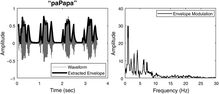
AEMS involves the spectral analysis of low-rate amplitude modulations within the envelope of the speech signal. The analysis covers the entire amplitude modulation spectrum as well as specific frequency bands of amplitude modulations. Fourier analysis is applied to the speech envelopes to identify the dominant amplitude modulation rate (Figure 40.1) (for different metrics, see Chapters 9, 10, and 30).
AEMS.
The left graph shows the amplitude-normalized waveform and the amplitude envelope (dark solid line) of a male saying “paPapa” four times. The right graph is its corresponding down-sampled envelope modulation spectrum (in dB).
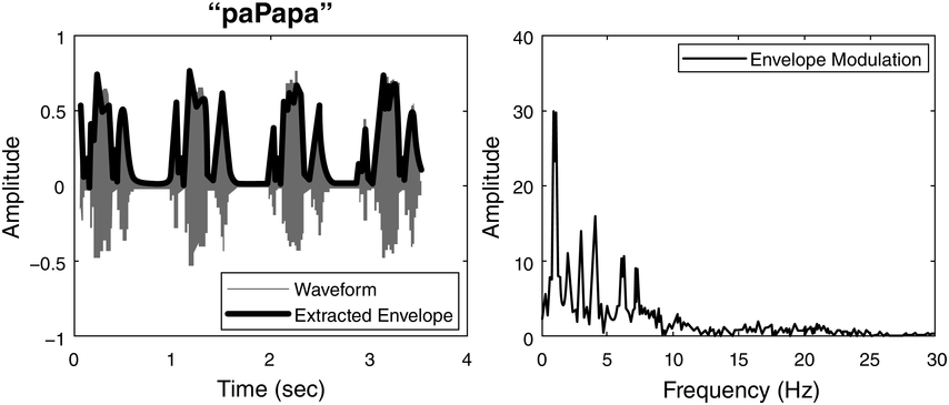
Figure 40.1 Long description
Left. The horizontal axis represents time, which ranges from 0 to 4 seconds. The vertical axis represents an amplitude which ranges from minus 1 to 1. It plots a waveform. The waveform is outlined with the extracted waveform. Right. The horizontal axis represents frequency, which ranges from 0 to 30 hertz. The vertical axis represents the amplitude, which ranges from 0 through 40. It plots a fluctuating line for envelope modulation.
In Figure 40.1, the left graph illustrates the amplitude envelope of a speech waveform (composed of four repetitions of /paPApa/ tri-syllabic nonsense words). This envelope captures temporal fluctuations in amplitude, including those corresponding to syllabic patterns. Regular patterns such as stressed-unstressed rhythms are also discernible. These regularities can be quantified by subjecting the envelope to Fourier analysis, resulting in a depiction of the dominant amplitude modulation rates present in the signal, as shown in the right graph. Note that the highest energy peak (in decibels) occurs at 1 Hz, with additional peaks observable at higher rates.
To generate the AEMS, the signal undergoes several processing steps. First, it is filtered into seven-octave bands using eighth-order Chebyshev digital filters, with center frequencies of 125, 250, 500, 1,000, 2,000, 4,000, and 8,000 Hz. Next, the amplitude envelope is extracted (half-wave rectified, then low-pass filtered at 30 Hz using a fourth-order Butterworth filter), and down-sampled to 80 Hz (mean subtracted) from the full signal and each of the seven-octave bands.
For each down-sampled envelope, a power spectrum analysis is performed using a 512-point fast Fourier transform, applying a Tukey window. The results are converted to decibels for frequencies up to 10 Hz (normalized to maximum autocorrelation). Consequently, seven EMS metrics are computed for each band and one metric from the full signal, resulting in a total of 56 metrics [(7 octave bands + 1 full signal) × 7 metrics]. All amplitude measures are normalized to the average amplitude across the spectrum. Table 40.2 illustrates the seven metrics and their descriptions.
Description of AEMS metrics.
| Metric | Description |
|---|---|
| Centroid | The frequency at which the amplitude of the spectrum is balanced. The period of this frequency corresponds to the duration of the dominant repetitive amplitude pattern. |
| Peak frequency | The frequency of the peak in the spectrum with the greatest amplitude. |
| Peak amplitude | The amplitude of the peak frequency described above (normalized by the overall amplitude of energy in the spectrum). This measurement indicates the extent to which the rhythm is influenced by a single frequency. |
| E3–6 | Energy in the region of 3–6 Hz (normalized). This corresponds to the approximate spectral range around 4 Hz, which has shown correlations with intelligibility (Houtgast and Steeneken, Reference Houtgast and Steeneken1985) and an inverse correlation with segmental deletions (Tilson and Johnson, Reference Tilsen and Johnson2008). |
| Below4 | Energy in spectrum from 0–4 Hz (normalized). The spectrum was divided at 4 Hz, as it has been suggested that the energy below and above 4 Hz exhibited relatively low correlation across diverse speakers and sentences. |
| Above4 | Energy in spectrum from 4–10 Hz (normalized). |
| Ratio4 | Energy below 4 Hz/energy above 4 Hz (normalized). |
40.2.4 Data Processing and Analysis
The values of each AEMS for each sentence and frequency band underwent outlier examination (± 2SD) based on group and speaking rate. Outliers were excluded before proceeding with statistical analyses. In total, 4.1% of the data (N=93,967) were eliminated. All statistical analyses were conducted using SPSS (Version 29).
40.2.5 Analysis: Stepwise Discrimination Analysis
Stepwise discriminant function analyses were carried out to evaluate the categorization of German-accented and French-accented English as native English utterances; English-accented German and French-accented German as native German utterances; and native German-accented French utterances as native French. These analyses were performed for each of the five speaking rates as well as for all rates combined.
Following the methodologies outlined by Liss et al. (Reference Liss, LeGendre and Lotto2010) and Wayland and Nozawa (Reference Wayland and Nozawa2019), in each step of the analysis, the parameter that minimized Wilks’ lambda was incorporated if the change’s F statistic was statistically significant at p < 0.05. Furthermore, any parameter that ceased to significantly decrease Wilks’ lambda (p > 0.10) upon adding a new variable was excluded from the discriminant function analysis. The outcome of this analysis yielded canonical functions, which signify linear combinations of the chosen predictor variables. These functions were subsequently utilized to establish classification rules for determining group membership, encompassing categories such as native English, German-accented English, French-accented English, native German, English-accented German, and French-accented German. The accuracy rate was expressed as a percentage.
To assess the robustness of the classification rules, leave-one-out cross-validation was employed. This involved classifying the excluded utterances based on the functions derived from all other utterances.
Finally, positive predictive values (PPVs) were calculated for the L2-accented utterances. These values represent the percentage of correctly predicted cases with the observed characteristic compared to the total number of cases predicted as having the characteristic. For example, PPVs for German-accented English indicate the percentage of German-accented English utterances that were correctly predicted to be native English, as a percentage of all utterances in the analysis classified as native English.
40.3 Results
Table 40.3 displays the cross-validated PPVs for German-accented English and French-accented English across the five speaking rates, as well as when all rates were considered together. The PPVs for German-accented English are consistently higher than those for French-accented English across all five rates. This suggested that a larger proportion of German-accented English utterances were categorized as English. A two-tailed independent T-test was conducted comparing PPVs across the five rates and confirmed that the difference was statistically significant [t(8) = 5.94, p < .001].
PPVs for German-accented English and French-accented English in terms of their classification as English based on EMS metrics.
| Metric | Accented type | Speaking rate | PPV (%) |
|---|---|---|---|
| EMS | German-accented English | slowest | 34.0 |
| slow | 36.1 | ||
| normal | 37.5 | ||
| fast | 42.4 | ||
| fastest | 51.2 | ||
| all rates combined | 32.2 | ||
| French-accented English | slowest | 6.0 | |
| slow | 5.6 | ||
| normal | 25.0 | ||
| fast | 12.1 | ||
| fastest | 2.4 | ||
| all rates combined | 9.1 |
PPVs for English-accented German and French-accented German are shown in Table 40.4. English-accented German was classified as German at a higher percentage than French-accented German for each rate and when all the rates were combined. The difference was statistically significant [t(8) = 6.02, p<.001].
PPVs for English-accented German and French-accented German in terms of their classification as German based on EMS metrics
| Metric | Accented type | Speaking rate | PPV (%) |
|---|---|---|---|
| EMS | English-accented German | slowest | 12.2 |
| slow | 10.0 | ||
| normal | 18.4 | ||
| fast | 16.7 | ||
| fastest | 14.7 | ||
| all rates combined | 11.7 | ||
| French-accented German | slowest | 1.1 | |
| slow | 1.4 | ||
| normal | 5.7 | ||
| fast | 4.9 | ||
| fastest | 4.9 | ||
| all rates combined | 6.1 |
Out of the 56 predictors, 11 were found to be statistically significant in the combined-rate discriminant function analysis (DFA) model. The primary predictor among these was Ratio4_125, denoting the normalized energy below 4 Hz to the energy above 4 Hz in the 125 Hz frequency band. In the DFA models for each of the five rates, the number of significant predictors varied: one for the normal rate, three for the fast rate, four for both the slow and fastest rates, and five for the slowest rate, with no overlap in the top predictor.
In the combined-rate DFA model, nine significant predictors emerged, with E3–6_2000, which represents energy in the range of 3–6 Hz (normalized by overall spectrum amplitude) from the 2,000 Hz band, being the top predictor. In the individual rate models, three–nine significant predictors were identified.
Table 40.5 shows PPVs for German-accented English as English and German-accented French as French. The difference was statistically significant [t(8) = 3.46, p = .009], indicating that German-accented English was classified as English significantly more frequently than German-accented French as French.
PPVs for German-accented English and German-accented French in terms of their classification as English and French, respectively, based on EMS metrics.
| Metric | Accented type | Speaking rate | PPV (%) |
|---|---|---|---|
| EMS | German-accented English | slowest | 28.9 |
| slow | 39.0 | ||
| normal | 44.4 | ||
| fast | 36.6 | ||
| fastest | 42.6 | ||
| all rates combined | 41.5 | ||
| German-accented French | slowest | 12.0 | |
| slow | 18.2 | ||
| normal | 28.9 | ||
| fast | 24.1 | ||
| fastest | 31.3 | ||
| all rates combined | 20.6 |
The combined-rate DFA model resulted in 14 significant predictors, with Peak amplitude-4000 being the top predictor. This predictor represents the amplitude of the frequency peak in the spectrum from the 4,000 Hz band. In the separate rate models, a varying combination of six–nine significant predictors was identified for the five different rates.
40.4 Discussion
The aim of the study was to examine the potential influence of shared linguistic rhythm on the acquisition of rhythm in an L2. The employed rhythm metrics analyzed temporal regularities extracted from the AEMS. These metrics capture low-rate temporal variations in spectral envelope amplitude, corresponding to prosodic units such as syllables, and regular durational variations such as stressed-unstressed intervals. Both different L1–L2 language combinations (German-accented versus French-accented English, and English-accented German versus French-accented German) and the same L1–L2 combination (German-accented English versus German-accented French) were explored.
The findings strongly support the advantage of the shared-L1 rhythm hypothesis, demonstrating that German-accented English is consistently more likely to be classified as English compared to French-accented English. Furthermore, German-accented English is classified as being closer to native English than German-accented French is to native French.
Interestingly, the results align with the word-based acoustic distance estimations derived from self-supervised neural models. These suggest that the word-level pronunciation of English by German speakers is closer to native English than that of French speakers. Similarly, English speakers show a closer word-based pronunciation to native German than to French. Furthermore, German speakers exhibit a closer pronunciation to English than to French. Together, the findings suggest that rhythm planning may be influenced by the words and their segmental makeup in the utterance (Myers and Watson, Reference Myers and Watson2021).
The significance of various predictors identified in the DFA models offers valuable insights into the acoustic features that contribute to the observed rhythmic classification patterns. For example, energy below 4 Hz was the primary predictor for differentiating between German-accented and French-accented English. Notably, predictor values were 1.9 for German-accented English and 2.8 for French-accented English. This indicates that in the 125 Hz octave band frequency (ranging from 88 to 177 Hz), the spectral envelope amplitude modulation rates below 4 Hz are more pronounced (relative to those above 4 Hz) in English spoken by French speakers than in that spoken by German speakers. An amplitude modulation rate of 4 Hz is typically associated with syllable-pattern information in speech, as noted by Greenberg et al. (Reference Greenberg, Carvey, Hitchcock and Chang2003) and Greenberg (Reference Greenberg, Greenberg and Ainsworth2006). These findings suggest that French-accented English exhibits a stronger presence of regular temporal patterns associated with prosodic units of or closer to a syllable size, reflecting a possible influence from French’s traditionally classified syllable-timed rhythm.
On the other hand, energy in the range of 3–6 Hz emerged as the top predictor for English-accented versus French-accented German. The 3–6 Hz range roughly corresponds to the spectral region around 3–4 Hz, which has been shown to correlate with vowel deletions, particularly in English (Tilsen and Johnson, Reference Tilsen and Johnson2008). Crucially, the predictor value was higher for English-accented German compared to French-accented German (4.5 versus 3.8). The higher values for English-accented German may thus be due to a greater amount of vowel deletion in German produced by English speakers compared to French-accented German.
Lastly, it is worth noting that top predictors and various combinations of significant predictors were identified for different speaking rates, indicating potential variations in rhythm articulation adjustments across varying rates of speech production. Further research is necessary to fully elucidate the relationship between these predictor patterns and the dynamic nature of speech rhythm under different speech tempos.
In conclusion, despite its extensive history of progress, research on speech rhythm continues to be exploratory due to the complexity of the underlying phenomena and the lack of an effective tool that bridges the gap between linguists’ intuition and tangible statistical patterns in the speech signal (Deloche et al., Reference Deloche, Bonnasse-Gahot and Gervain2024). Our findings not only support the facilitating roles of shared linguistic rhythm in L2 speech learning but also underscore the AEMS’s significant potential as a powerful tool for analyzing speech rhythms, both within and across languages. Its ability to capture regular patterns across various speech unit sizes uniquely positions it to reveal nuanced rhythmic differences overlooked by traditional methods focused solely on segmental intervals. In addition, the AEMS approach is automated, thus avoiding the labor-intensive and error-prone process required for segmenting speech into vocalic and consonantal intervals.
40.5 Acknowledgments
We express our gratitude to Professor Volker Dellwo for his generosity in sharing the BonnTempo corpus. We also extend our appreciation to Professor Andrew Lotto for providing the MatLab codes for the EMS metrics, and to Professor Yonghee Oh for providing Figure 40.1.
Summary
Using metrics extracted from the AEMS, this study demonstrated the facilitating roles of shared linguistic rhythm and established the AEMS as a powerful tool for analyzing speech rhythms, both within and across languages.
Implications
To fully understand the complexity of linguistic rhythm, it is crucial to employ metrics capable of quantifying temporal patterns across various speech unit sizes. Automated tools such as the AEMS significantly enhance our ability to examine rhythm within and across languages, facilitating a more nuanced understanding of the connection between linguists’ intuition and tangible statistical patterns in the speech signal.
Gains
The acquisition of L2 rhythm is facilitated by a shared L1 rhythm, with improved L2 rhythm production correlating to enhanced word/subword production in L2. This observation supports the notion that planning metrical representations for rhythm also depends on the words and their segmental composition in the spoken utterance.

 Open access