


Impact Statement
Researchers across fields have long pondered over the question of how and why fish school in specific crystallized formations in a flow. We attempt to answer this question from a purely hydrodynamic standpoint in a two-fish subsystem of a school, swimming against a channel flow. Through an elegant mathematical model, derived based on fundamental fluid dynamics principles, we demonstrate the emergence of unique schooling patterns that are stable to disturbances. Interestingly, we find that two fish, swimming in close proximity but not precisely side-by-side, always orient opposite to the flow direction through passive hydrodynamics, without any active feedback/sensory mechanism. Our findings provide theoretical evidence of stable configurations of schooling and their dependence on flow conditions and streamwise interfish distance. The proposed model and developed insights not only advance our understanding of a fundamental form of collective behaviour but will also guide future experimental design and investigation of live/robotic fish schools.
1. Introduction
Rheotaxis is the ability of a fish to orient and swim against an oncoming flow. At first, visual cues were considered to be the dominant contributor towards rheotaxis (Reference ArnoldArnold, 1974). Later, experiments revealed that fish exhibit this behaviour even in the absence of vision (Reference Champalbert and MarchandChampalbert & Marchand, 1994; Reference Suli, Watson, Rubel and RaibleSuli, Watson, Rubel, & Raible, 2012), which has led researchers to investigate additional sensory systems that fish may employ to appraise the flow environment. Reference Suli, Watson, Rubel and RaibleSuli et al. (2012) and Reference Oteiza, Odstrcil, Lauder, Portugues and EngertOteiza, Odstrcil, Lauder, Portugues, and Engert (2017) showed that fish use their lateral lines (Reference Montgomery, Baker and CartonMontgomery, Baker, & Carton, 1997), a mechanosensory organ, to detect gradients of the surrounding flow velocity and adjust their orientation accordingly. This lateral line-mediated rheotaxis was markedly evident in the presence of non-uniform flows (Reference Kulpa, Bak-Coleman and CoombsKulpa, Bak-Coleman, & Coombs, 2015; Reference Oteiza, Odstrcil, Lauder, Portugues and EngertOteiza et al., 2017), while much reduced in zero-gradient uniform flows (Reference Bak-Coleman and CoombsBak-Coleman & Coombs, 2014; Reference Bak-Coleman, Court, Paley and CoombsBak-Coleman, Court, Paley, & Coombs, 2013). Aside from gradients, the rheotactic behaviour of fish is also affected by the speed of the flow (Reference Bak-Coleman, Court, Paley and CoombsBak-Coleman et al., 2013), whereby the ability to orient against a flow is limited at low flow speeds. While visual and lateral line sensing play a key role in the occurrence of rheotaxis, recent work suggests that the basis of rheotaxis should be sought in the integration of multiple senses, including tactile senses and vestibular system (Reference Coombs, Bak-Coleman and MontgomeryCoombs, Bak-Coleman, & Montgomery, 2020).
Another potentially significant contributor in the phenomenon of rheotaxis is the passive hydrodynamic mechanisms affecting the fish swimming. As the recent comprehensive review of rheotaxis by Reference Coombs, Bak-Coleman and MontgomeryCoombs et al. (2020) states, one of the questions that remains unanswered is: ‘What role, if any, do passive (e.g. wind vane) mechanisms play in rheotaxis and how are these influenced by fish factors (e.g. body shape) and flow dynamics?’ In this vein, Reference Porfiri, Zhang and PetersonPorfiri, Zhang, and Peterson (2022) recently developed a hydrodynamic model for a fish swimming in a channel flow, providing the first analytical justification of rheotaxis by purely hydrodynamic mechanisms in the absence of any sensory feedback. Their model is the first to analyse rheotaxis as a bidirectional fluid–structure interaction problem, in which the fish modifies the surrounding flow field and the flow field, in turn, affects fish swimming. These bidirectional interactions are pervasive in fluid mechanics, from fluid–structure interactions in vortex-induced vibrations (Reference Williamson and GovardhanWilliamson & Govardhan, 2004) to laminar boundary layer response to environmental disturbances (Reference Saric, Reed and KerschenSaric, Reed, & Kerschen, 2002), yet mathematical modelling of rheotaxis and swimming in general have largely discounted them.
This work seeks to understand the implications of the passive hydrodynamic pathway discovered in Reference Porfiri, Zhang and PetersonPorfiri et al. (2022) on fish schooling. Schooling refers to the coordinated swimming of fish in close proximity in crystallized spatial formations, as exhibited by most fish species (Reference Filella, Nadal, Sire, Kanso and EloyFilella, Nadal, Sire, Kanso, & Eloy, 2018; Reference Kalueff, Gebhardt, Stewart, Cachat, Brimmer, Chawla and LandsmanKalueff et al., 2013; Reference ShawShaw, 1978). Different patterns of fish schooling that are often shown to emerge include side-by-side (phalanx), in-line and staggered (diamond) formations (Reference Daghooghi and BorazjaniDaghooghi and Borazjani, 2015; Reference Hemelrijk, Reid, Hildenbrandt and PaddingHemelrijk et al., 2015; Reference Oza, Ristroph and ShelleyOza, Ristroph, & Shelley, 2019; Reference Park and SungPark & Sung, 2018; Reference Thandiackal and LauderThandiackal & Lauder, 2022; Reference WeihsWeihs, 1973). One approach to explain schooling is based on the premise of collective energy savings so that fish arrange their positions with respect to their neighbours in an attempt to reduce their swimming costs (Reference Ashraf, Bradshaw, Ha, Halloy, Godoy-Diana and ThiriaAshraf et al., 2017; Reference Liao, Beal, Lauder and TriantafyllouLiao, Beal, Lauder, & Triantafyllou, 2003a; Reference Maertens, Gao and TriantafyllouMaertens et al., 2017; Reference Marras, Killen, Lindström, McKenzie, Steffensen and DomeniciMarras et al., 2015). Another approach to understand schooling patterns is based on the Lighthill conjecture (Reference Cong, Teng and ChengCong, Teng, & Cheng, 2020; Reference Dai, He, Zhang and ZhangDai, He, Zhang, & Zhang, 2018; Reference Kurt, Ormonde, Mivehchi and MooredKurt, Ormonde, Mivehchi, & Moored, 2021; Reference LighthillLighthill, 1975; Reference Lin, Wu, Zhang and YangLin, Wu, Zhang, & Yang, 2019; Reference Peng, Huang and LuPeng, Huang, & Lu, 2018), which postulates that orderly patterns in a school emerge due to flow-mediated passive forces. The focus of this study is on investigating the role of the latter in the context of fish schooling and rheotaxis, which leads to the formation of stable schooling patterns in fish swimming against a flow.
Towards this aim, we focus on a fish pair as a minimalistic instance of a school. Experimental studies involving pairs of live fish have shown evidence for specific schooling configurations, such as side-by-side (Reference Ashraf, Godoy-Diana, Halloy, Collignon and ThiriaAshraf, Godoy-Diana, Halloy, Collignon, & Thiria, 2016; Reference Chicoli, Butail, Lun, Bak-Coleman, Coombs and PaleyChicoli et al., 2014) as well as in-line (Reference Thandiackal and LauderThandiackal & Lauder, 2022) configurations, when swimming against a flow. Recent work by Reference De Bie, Manes and KempDe Bie, Manes, and Kemp (2020) has further shown that pairs of fish tend to swim in-line in placid water, side-by-side in a high speed flow, and without any identifiable pattern in a low-speed flow. Examining the combined effect of flow (hydrodynamic interaction) and illumination (visual interaction) on fish collective behaviour, Reference Lombana and PorfiriLombana and Porfiri (2022) provided evidence that the relative time spent by a pair in a side-by-side configuration increases in the presence of flow as well as in the presence of light. However, in these studies the different forms of interactions (visual, hydrodynamic and tactile) are intermingled, and the specific role of hydrodynamics is difficult to tease out. Detailing the role of hydrodynamics through sensory deprivation may not be completely reliable due to the possible pitfalls of such methodologies, such as disabling certain senses, even if perfectly executed, may affect the overall behaviour of the fish and deprivation of one sense may cause the other senses to over-compensate (Reference Coombs, Bak-Coleman and MontgomeryCoombs et al., 2020).
To isolate the role of hydrodynamics, researchers have also proposed the study of a pair of pitching airfoils as a proxy subsystem of a fish school against an oncoming flow. For example, Reference Bao and TaoBao and Tao (2014), Reference Boschitsch, Dewey and SmitsBoschitsch, Dewey, and Smits (2014), Reference Kurt and MooredKurt and Moored (2018) and Reference Saadat, Berlinger, Sheshmani, Nagpal, Lauder and Haj-HaririSaadat et al. (2021) have shown evidence in support of in-line swimming, while Reference Dewey, Quinn, Boschitsch and SmitsDewey, Quinn, Boschitsch, and Smits (2014) and Reference Gungor and HemmatiGungor and Hemmati (2021) have shown increased efficiency in side-by-side swimming. Experiments and numerical simulations of self-propelled flapping wings and plates (Reference Becker, Masoud, Newbolt, Shelley and RistrophBecker, Masoud, Newbolt, Shelley, & Ristroph, 2015; Reference Newbolt, Zhang and RistrophNewbolt, Zhang, & Ristroph, 2019; Reference Ramananarivo, Fang, Oza, Zhang and RistrophRamananarivo, Fang, Oza, Zhang, & Ristroph, 2016) indicate that orderly formations in schools may emerge simply through flow interactions, and that hydrodynamic mechanisms may be enough to support a group's collective motion. These, along with other studies (Reference Baddoo, Moore, Oza and CrowdyBaddoo, Moore, Oza, & Crowdy, 2021; Reference Kurt, Ormonde, Mivehchi and MooredKurt et al., 2021; Reference Lin, Wu, Zhang and YangLin et al., 2019), have investigated the stability of spatial configurations of such schooling systems via experimental measurements and/or numerical predictions of hydrodynamic forces. Reference Kurt, Ormonde, Mivehchi and MooredKurt et al. (2021) and Reference Peng, Huang and LuPeng et al. (2018) have shown propensity for a stable side-by-side configuration in pitching airfoils and plates, while Reference Newbolt, Zhang and RistrophNewbolt et al. (2019) and Reference Lin, Wu, Zhang and YangLin et al. (2019) provide evidence of stable configurations in two hydrofoils swimming in tandem. These studies suggest the existence of multistable formations of schooling, and that transitions between such stable states may be induced by applying external perturbations to the swimmers (Reference Newbolt, Zhang and RistrophNewbolt, Zhang, & Ristroph, 2022).
To gain a fundamental understanding of the hydrodynamic foundations of such schooling formations, we propose to investigate the problem from a theoretical perspective that complements the experimental and computational findings in the literature. We consider a fish pair swimming in an infinite channel. First, we develop a mathematical model of the positions and orientations of both the fish by considering all the passive hydrodynamic interactions in the system. The behaviour of each fish is modelled as a vortex dipole in a two-dimensional flow under the finite-dipole paradigm of Reference Tchieu, Kanso and NewtonTchieu, Kanso, and Newton (2012), which has been extensively used in the past to study the hydrodynamics of swimming animals (Reference Filella, Nadal, Sire, Kanso and EloyFilella et al., 2018; Reference Gazzola, Tchieu, Alexeev, de Brauer and KoumoutsakosGazzola, Tchieu, Alexeev, de Brauer, & Koumoutsakos, 2016; Reference Kanso and TsangKanso & Tsang, 2014; Reference Porfiri, Karakaya, Sattanapalle and PetersonPorfiri, Karakaya, Sattanapalle, & Peterson, 2021; Reference Porfiri, Zhang and PetersonPorfiri et al., 2022). Instead of considering a fish to be a passive body that does not affect the flow, we model their effect on the background flow in the presence of the channel walls (Reference Porfiri, Zhang and PetersonPorfiri et al., 2022). This results in a five-dimensional dynamical system for the fish pair in the channel flow, characterized by bidirectional couplings between the two fish and the fluid flow.
We use the proposed model to elucidate the hydrodynamic mechanisms driving the formation of schooling patterns in the presence of a flow. We study the properties and equilibria of the dynamical system, and their significance in schooling and rheotactic behaviour of the fish. Linear stability analysis is performed to demonstrate the existence of specific stable configurations of the fish pair, both in terms of their positions and orientations. The system's equilibria are shown to depend on the flow curvature and the streamwise distance between the fish. Finally, the study evaluates the role played by lateral line sensing and the effect of varying channel widths on the stability of schooling configurations. The rest of the paper is organized as follows. In § 2, we present the mathematical model; in § 3, we present the results of all the analysis; and finally, conclusions from the analysis are discussed in § 4 along with limitations of the research.
2. Mathematical model
First, we derive a mathematical model of passive hydrodynamic interaction between two fish swimming in an infinite channel of width  $h$ with an imposed flow. A schematic diagram of the set-up is illustrated in figure 1. At any time $t$, the two-dimensional positions of the two fish (labelled 1 and 2) in a Cartesian coordinate system $(x;y)$ are given by $\boldsymbol {r}_1(t)=x_1(t)\hat {\boldsymbol {i}}+y_1(t)\hat {\boldsymbol {j}}$ and $\boldsymbol {r}_2(t)=x_2(t)\hat {\boldsymbol {i}}+y_2(t)\hat {\boldsymbol {j}}$, respectively, and their heading directions are specified by the angles, $\theta _1(t)$ and $\theta _2(t)$, with respect to the positive $x$ direction. Here, $\hat {\boldsymbol {i}}$ is the unit vector of the streamwise coordinate $x$, and $\hat {\boldsymbol {j}}$ is the unit vector of the cross-stream coordinate $y$. We consider that the two fish are identical in size and have the same swimming capacity, that is, they propel themselves by tail-beating at the same amplitude and frequency. Therefore, their self-propulsion velocities at a time $t$ are given by
 \begin{equation} \boldsymbol{v}_k (\theta_k) = v_0(\cos{\theta_k} \hat{\boldsymbol{i}} + \sin{\theta_k} \hat{\boldsymbol{j}}), \quad \text{where } k = 1,2. \end{equation}
Here,  $v_0$ is the constant self-propelling speed of the fish and the direction of the fish's self-propulsion is given by the unit vector $\hat {\boldsymbol {v}}_k (\theta _k(t))= \cos {\theta _k(t)} \hat {\boldsymbol {i}} + \sin {\theta _k(t)} \hat {\boldsymbol {j}}$.
Schematic of two interacting fish swimming against a flow inside a channel of width  $h$, with $x$ and $y$ being streamwise and cross-stream coordinates, respectively. Note that the flow is in the (positive) $x$ direction.

2.1 Modelling the fluid flow
Each fish is modelled as a vortex dipole (Reference Tchieu, Kanso and NewtonTchieu et al., 2012), a representation that has previously been used in several studies of fish schooling (Reference Filella, Nadal, Sire, Kanso and EloyFilella et al., 2018; Reference Gazzola, Tchieu, Alexeev, de Brauer and KoumoutsakosGazzola et al., 2016), and has been validated with experimental observations (Reference Porfiri, Karakaya, Sattanapalle and PetersonPorfiri et al., 2021) as well as numerical simulations (Reference Porfiri, Zhang and PetersonPorfiri et al., 2022; Reference Zhang, Peterson and PorfiriZhang, Peterson, & Porfiri, 2023). The mean flow field generated by the swimming fish is modelled using potential flow, wherein the potential field due to the self-propelling motion of each fish is given by
 \begin{equation} \phi_{f_k} (\boldsymbol{r},\boldsymbol{r}_k,\theta_k) = {-} r_0^2 \frac{(\boldsymbol{r}-\boldsymbol{r}_k) \boldsymbol{\cdot} \boldsymbol{v}_k}{\lVert \boldsymbol{r} - \boldsymbol{r}_k \rVert^2},\quad \text{for }k = 1,2, \end{equation}
where  $\boldsymbol {r}=x \hat {\boldsymbol {i}} + y \hat {\boldsymbol {j}}$. These are the far-field representation of the dipoles (Reference Filella, Nadal, Sire, Kanso and EloyFilella et al., 2018) under the assumption that the dipole length scale ( $r_0$) is much smaller than the flow length scale, that is, $r_0 \ll h$, where $h$ is the channel width. The flow velocity induced by the point dipoles are then given by ${\boldsymbol {u}_{f}}_k = \boldsymbol {\nabla } \phi _{f_k}$, for
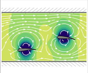
  $k=1,2$ (see supplementary material S1 available at https://doi.org/10.1017/flo.2023.25 for complete expressions). Figure 2(a) shows the flow streamlines generated by the dipoles ( ${\boldsymbol {u}_{f}}_1 + {\boldsymbol {u}_{f}}_2$) in a quiescent fluid in an unbounded domain. These streamlines approximately replicate the inviscid flow due to the self-propelling body of a fish, emanating from the head and circulating towards the tail of the fish (Reference Tchieu, Kanso and NewtonTchieu et al., 2012; Reference Zhang, Peterson and PorfiriZhang et al., 2023). It is further evident from the figure that if the two fish are in close proximity, their individually generated streamline patterns are influenced by each other.
Predicted flow streamlines around two fish swimming (a) in a quiescent fluid within an unbounded domain, (b) in a quiescent fluid bounded by channel walls and (c) against a flow ( $U_0=2, \epsilon =0.1$) bounded by channel walls.

The dipole-generated streamlines are further affected by the walls, which are represented by streamlines generated via the method of images (Reference NewtonNewton, 2001) by using fictitious fish (dipoles) mirrored with respect to the wall plane (note that in reality the fluid is viscous, in which case a no-slip boundary condition must also be satisfied at the walls; but as a simplification, we assume the flow to be inviscid and only account for the zero wall-normal velocity at the walls). In the presence of two parallel walls at  $y=0$ and $y=h$, this results in an infinite number of such image dipoles on either side of the channel, as shown by Reference Porfiri, Zhang and PetersonPorfiri et al. (2022). The infinite sum of the potential fields generated by such image dipoles of both fish yields the following potential field (Reference Porfiri, Zhang and PetersonPorfiri et al., 2022):
 \begin{align}
\phi_{w} (\boldsymbol{r},\boldsymbol{r}_1,\boldsymbol{r}_2,\theta_1,\theta_2)
& = \sum_{k = 1,2} \frac{{v_0} r_0^2}{4} \left[ 4 \frac{(x-x_k)\cos{\theta_k} +
(y-y_k)\sin{\theta_k}}{(x-x_k)^2 + (y-y_k)^2}\right.
\nonumber\\ &\quad -\left. \frac{\rm \pi}{h} ( {\rm
e}^{\mathrm{i} \theta_k} (\coth{{\rm \pi} A} + \coth{{\rm \pi} B^ *
}) + {\rm e}^{-\mathrm{i} \theta_k}(\coth{{\rm \pi} A^ * } +
\coth{{\rm \pi} B}) ) \vphantom{\frac{(x-x_k)\cos{\theta_k} +
(y-y_k)\sin{\theta_k}}{(x-x_k)^2 + (y-y_k)^2}}\right] ,
\end{align}
\begin{align}
\phi_{w} (\boldsymbol{r},\boldsymbol{r}_1,\boldsymbol{r}_2,\theta_1,\theta_2)
& = \sum_{k = 1,2} \frac{{v_0} r_0^2}{4} \left[ 4 \frac{(x-x_k)\cos{\theta_k} +
(y-y_k)\sin{\theta_k}}{(x-x_k)^2 + (y-y_k)^2}\right.
\nonumber\\ &\quad -\left. \frac{\rm \pi}{h} ( {\rm
e}^{\mathrm{i} \theta_k} (\coth{{\rm \pi} A} + \coth{{\rm \pi} B^ *
}) + {\rm e}^{-\mathrm{i} \theta_k}(\coth{{\rm \pi} A^ * } +
\coth{{\rm \pi} B}) ) \vphantom{\frac{(x-x_k)\cos{\theta_k} +
(y-y_k)\sin{\theta_k}}{(x-x_k)^2 + (y-y_k)^2}}\right] ,
\end{align}
where  $A=((x-x_k)+\mathrm {i}(y-y_k))/(2h)$, $B=((x-x_k)+\mathrm {i}(y+y_k))/(2h)$, $\mathrm {i}$ is the imaginary unit, and superscript $*$ represents complex conjugation. Thus, the velocity field can be obtained by $\boldsymbol {u}_{\boldsymbol {w}} = \boldsymbol {\nabla } \phi _w$ (see supplementary material S1 for complete expression). The resultant flow streamlines due to the fish swimming between the walls of a channel ( ${\boldsymbol {u}_{f}}_1 + {\boldsymbol {u}_{f}}_2 + \boldsymbol {u}_w$) are illustrated in figure 2(b). Near the walls, the streamlines reorient to become parallel to the wall, creating large-circulatory motions about the fish.
To mimic a background flow inside a channel, we add a weakly rotational velocity profile across the channel,
 \begin{equation} \boldsymbol{u}_b(\boldsymbol{r}) = U_0 \biggl( 1-4\epsilon \left( \frac{y}{h} - \frac{1}{2} \right)^2 \biggr) \hat{\boldsymbol{i}}, \end{equation}
where  $U_0$ is the maximum flow velocity at the channel centreline and $\epsilon$ is a positive parameter controlling the curvature of the velocity profile, and thus the vorticity in the flow. For $\epsilon \rightarrow 0$, we approach a nearly uniform irrotational background flow, while $\epsilon = 1$ yields the parabolic profile of laminar flow in a channel (plane Poiseuille flow). If $0< \epsilon \ll 1$, the background flow closely resembles the mean velocity profile of a realistic turbulent channel flow with a small curvature near centreline but does not satisfy the no-slip condition at the walls. Superposing the background flow velocity on the velocity field generated by the fish in the presence of the walls yields the following total flow velocity at any location $\boldsymbol {r}$ of the flow domain:
 \begin{equation} \boldsymbol{u}(\boldsymbol{r},\boldsymbol{r}_1,\boldsymbol{r}_2,\theta_1,\theta_2) = {\boldsymbol{u}_f}_1 (\boldsymbol{r},\boldsymbol{r}_1,\theta_1) + {\boldsymbol{u}_f}_2 (\boldsymbol{r},\boldsymbol{r}_2,\theta_2) + \boldsymbol{u}_w (\boldsymbol{r},\boldsymbol{r}_1,\boldsymbol{r}_2,\theta_1,\theta_2) + \boldsymbol{u}_b (\boldsymbol{r}).\end{equation}
The resultant flow streamlines are illustrated in figure 2(c).
2.2 Modelling fish dynamics
The translational motion of a fish can be obtained by the addition of the advection experienced by the fish due to the flow and its self-propulsion due to its own tail beating motion in the fluid. First, we determine the advection velocities ( $\boldsymbol {U}_1$ and $\boldsymbol {U}_2$) experienced by the two fish by desingularizing the total velocity field (2.5), that is, without considering the contribution of the dipole at its own location and obtaining the value at the location of the dipole in the limit form,
 \begin{gather} \boldsymbol{U}_1 (\boldsymbol{r}_1,\boldsymbol{r}_2,\theta_1,\theta_2) = \lim_{\boldsymbol{r} \rightarrow \boldsymbol{r}_1 } [ {\boldsymbol{u}_f}_2 (\boldsymbol{r},\boldsymbol{r}_2,\theta_2) + \boldsymbol{u}_w (\boldsymbol{r},\boldsymbol{r}_1,\boldsymbol{r}_2,\theta_1,\theta_2) + \boldsymbol{u}_b (\boldsymbol{r}) ] , \end{gather}
 \begin{gather}\boldsymbol{U}_2 (\boldsymbol{r}_1,\boldsymbol{r}_2,\theta_1,\theta_2) = \lim_{\boldsymbol{r} \rightarrow \boldsymbol{r}_2 } [ {\boldsymbol{u}_f}_1 (\boldsymbol{r},\boldsymbol{r}_1,\theta_1) + \boldsymbol{u}_w (\boldsymbol{r},\boldsymbol{r}_1,\boldsymbol{r}_2,\theta_1,\theta_2) + \boldsymbol{u}_b (\boldsymbol{r}) ] . \end{gather}
The complete expressions of the advection velocities experienced by the fish are presented in supplementary material S2. The velocity of each fish is therefore given by
 \begin{gather} \dot{\boldsymbol{r}}_1(t) = \boldsymbol{U_1}(\boldsymbol{r}_1(t),\boldsymbol{r}_2(t),\theta_1(t),\theta_2(t)) + \boldsymbol{v_1}(\theta_1(t)) , \end{gather}
 \begin{gather}\dot{\boldsymbol{r}}_2(t) = \boldsymbol{U_2}(\boldsymbol{r}_1(t),\boldsymbol{r}_2(t),\theta_1(t),\theta_2(t)) + \boldsymbol{v_2}(\theta_2(t)), \end{gather}
where the self-propulsion velocities of the fish,  $\boldsymbol {v}_1$ and $\boldsymbol {v}_2$, are given by (2.1).
The rotational motion of each fish (dipole) is attributed to the angular velocity induced by the flow field and the active sensing mechanism of the fish that helps them navigate the flow. The flow-induced turn-rate is due to the two vortices comprising the dipole experiencing different velocities. In the far-field limit for a transverse dipole, referred to as a T-dipole (Reference Kanso and TsangKanso & Tsang, 2014; Reference Porfiri, Karakaya, Sattanapalle and PetersonPorfiri et al., 2021, Reference Porfiri, Zhang and Peterson2022; Reference Tchieu, Kanso and NewtonTchieu et al., 2012), this angular velocity can be approximated from the gradient of flow velocity orthogonal to the dipole's velocity ( $\boldsymbol {v}_k$ for $k=1,2$) as follows (note that an alternative is the aligned dipole (A-dipole) treatment that mimics the response of a slender body to flow gradients (Reference Filella, Nadal, Sire, Kanso and EloyFilella et al., 2018; Reference Kanso and TsangKanso & Tsang, 2014)):
 \begin{align} \varOmega_1(\boldsymbol{r}_1,\boldsymbol{r}_2,\theta_1,\theta_2) & = {-} \hat{\boldsymbol{v}}_1(\theta_1). \left[ \lim_{\boldsymbol{r} \rightarrow \boldsymbol{r}_1}\right. \{ \boldsymbol{\nabla} ({\boldsymbol{u}_f}_2 (\boldsymbol{r},\boldsymbol{r}_2,\theta_2) \nonumber\\ &\quad + \boldsymbol{u}_w (\boldsymbol{r},\boldsymbol{r}_1,\boldsymbol{r}_2,\theta_1,\theta_2) + \boldsymbol{u}_b(\boldsymbol{r})) \}\left. \vphantom{\lim_{\boldsymbol{r}}} \boldsymbol{\hat{v}^{\perp}}_1(\theta_1) \vphantom{\lim_{\boldsymbol{r} \rightarrow \boldsymbol{r}_1}}\right], \end{align}
 \begin{align} \varOmega_2(\boldsymbol{r}_1,\boldsymbol{r}_2,\theta_1,\theta_2) & = {-} \hat{\boldsymbol{v}}_2(\theta_2). \left[ \lim_{\boldsymbol{r} \rightarrow \boldsymbol{r}_2} \right. \{ \boldsymbol{\nabla} ({\boldsymbol{u}_f}_1 (\boldsymbol{r},\boldsymbol{r}_1,\theta_1) \nonumber\\ &\quad + \boldsymbol{u}_w (\boldsymbol{r},\boldsymbol{r}_1,\boldsymbol{r}_2,\theta_1,\theta_2) + \boldsymbol{u}_b (\boldsymbol{r})) \}\left. \vphantom{\lim_{\boldsymbol{r}}} \boldsymbol{\hat{v}^{\perp}}_2(\theta_2) \vphantom{\lim_{\boldsymbol{r} \rightarrow \boldsymbol{r}_2}}\right], \end{align}
where  $\hat {\boldsymbol {v}}_k^{\perp }=-\sin {\theta _k}\hat {\boldsymbol {i}}+\cos {\theta _k}\hat {\boldsymbol {i}}$, for $k=1,2$, is the unit vector orthogonal to the fish's self-propelling direction. Complete expressions of the angular velocities are presented in supplementary material S2.
In addition to the passive hydrodynamic turning mechanism, a fish may undergo active rotation in response to local flow sensing through its lateral line (Reference Montgomery, Baker and CartonMontgomery et al., 1997). Studies have shown that this hydrodynamic feedback via a lateral line is related to the circulation of the flow surrounding the fish (Reference Oteiza, Odstrcil, Lauder, Portugues and EngertOteiza et al., 2017) and can be approximated by considering a linear feedback term (Reference Porfiri, Zhang and PetersonPorfiri et al., 2022) of the form  $\lambda (\boldsymbol {r}_k,\theta _k) = K \varGamma (\boldsymbol {r}_k,\theta _k)$, where $K$ is the feedback gain and $\varGamma$ is the circulation in a rectangular region ( $\mathcal {R}$) about the location of the fish, of width $r_0$ and length equal to the fish body length $l$. The circulation $\varGamma = \int _\mathcal {R} \boldsymbol {\omega } \boldsymbol {\cdot} \mathrm {d}\boldsymbol {A}$ can be determined by integrating the vorticity of the flow, $\boldsymbol {\omega }$, which is given by
 \begin{equation} \boldsymbol{\omega}(\boldsymbol{r}) = (\boldsymbol{\nabla} \times \boldsymbol{u_b}) = \frac{8 U_0 \epsilon}{h} \left( \frac{y}{h} - \frac{1}{2} \right)\boldsymbol{\hat{k}}, \end{equation}
since all other contributions to the velocity field are irrotational. As shown by Reference Porfiri, Zhang and PetersonPorfiri et al. (2022), the feedback angular velocity of each fish due to their lateral line sensing is given by
 \begin{equation} \lambda_k (\boldsymbol{r}_k,\theta_k) = \kappa \frac{8 U_0 \epsilon}{h} \left( \frac{y_k}{h} - \frac{1}{2} \right), \quad \text{for } k = 1,2,\end{equation}
where  $\kappa =K r_0 l$ is the non-dimensional lateral line feedback gain. Therefore, the total turn-rates of the two fish are obtained by adding the passive and active hydrodynamic effects discussed above, yielding the following two coupled ordinary differential equations:
 \begin{gather} \dot{\theta}_1(t) = \varOmega_1(\boldsymbol{r}_1(t),\boldsymbol{r}_2(t),\theta_1(t),\theta_2(t)) + \lambda_1(\boldsymbol{r}_1(t),\theta_1(t)), \end{gather}
 \begin{gather}\dot{\theta}_2(t) = \varOmega_2(\boldsymbol{r}_1(t),\boldsymbol{r}_2(t),\theta_1(t),\theta_2(t)) + \lambda_2(\boldsymbol{r}_2(t),\theta_2(t)), \end{gather}
where the flow-induced turn-rates are given in (2.8a) and (2.8b), and the feedback due to the lateral line is given by (2.10).
2.3 Dynamical system
Translational and rotational motion of the two fish in the channel is given by the system of six equations for  $x_1,y_1,x_2,y_2,\theta _1$, and $\theta _2$ ((2.7) and (2.11)). In order to study the dynamical system properties, we first non-dimensionalize these equations using the following non-dimensional quantities:
 \begin{equation} \xi_1 = \frac{y_1}{h} - \frac{1}{2} , \quad \xi_2 = \frac{y_2}{h} - \frac{1}{2} , \quad \varLambda = \frac{(x_1-x_2)}{h} , \quad t' = t \frac{v_0}{h} . \end{equation}
Here,  $\xi _1$ and $\xi _2$ are the non-dimensional cross-stream coordinates and $t'$ is the non-dimensional time coordinate. To study the spatial configurations of the fish pair, their exact streamwise locations ( $x_1,x_2$) in the infinite channel are inconsequential. Instead, the important variable is the streamwise distance between the two fish $(x_1-x_2)$, for which we introduce the non-dimensional streamwise distance $\varLambda$. The equations for location coordinates, (2.7a) and (2.7b), are non-dimensionalized by dividing both sides by $v_0$ (the self-propulsion speed of the fish), while the rate of change of orientation, (2.11a) and (2.11b), are non-dimensionalized by multiplying both sides by $h/v_0$. Upon non-dimensionalization, the following two additional non-dimensional parameters emerge:
 \begin{equation} \alpha = \frac{U_0 \epsilon}{v_0} \quad \text{and} \quad \rho = \frac{r_0}{h} , \end{equation}
where  $\alpha$ is a measure of the curvature ( $\epsilon$) and speed ( $U_0$) of the background flow with respect to the fish self-propulsion speed ( $v_0$), and $\rho$ represents the inverse of the channel width for a given fish size. The third parameter of the system is the non-dimensional lateral line feedback gain $\kappa$.
The final system of non-dimensional equations governing the dynamics of the two-fish configuration in the channel is given by
 \begin{gather} \dot{\xi_1} = \sin{\theta_1} + \rho^2 f_{\xi}(\xi_1,\xi_2,\theta_1,\theta_2,\varLambda), \end{gather}
 \begin{gather}\dot{\xi_2} = \sin{\theta_2} + \rho^2 f_{\xi}(\xi_2,\xi_1,\theta_2,\theta_1,-\varLambda), \end{gather}
 \begin{gather}\dot{\theta_1} = \alpha \xi_1 ( 8 \kappa + g_{\theta}(\xi_1,\theta_1)) + \rho^2 f_{\theta}(\xi_1,\xi_2,\theta_1,\theta_2,\varLambda), \end{gather}
 \begin{gather}\dot{\theta_2} = \alpha \xi_2 ( 8 \kappa + g_{\theta}(\xi_2,\theta_2)) + \rho^2 f_{\theta}(\xi_2,\xi_1,\theta_2,\theta_1,-\varLambda), \end{gather}
 \begin{gather}\dot{\varLambda} = (\cos{\theta_2}-\cos{\theta_1}) + 4 \alpha ( \xi_1^2 - \xi_2^2) + \rho^2 f_{\varLambda}(\xi_1,\xi_2,\theta_1,\theta_2,\varLambda), \end{gather}
where  $f_{\xi },f_{\theta },g_{\theta }$ and $f_{\varLambda }$ are complicated trigonometric functions of $(\xi _1,\xi _2,\theta _1,\theta _2,\varLambda )$ and their expressions are presented in supplementary material (S3). Here and in what follows, we omit the dependence on the non-dimensional time variable $t'$. There is a symmetry evident in the equations, which is expected as the two fish are assumed to be identical and their influences on each other through an inviscid hydrodynamic field are similar in form. Note that the equations for cross-stream coordinates ( $\xi _1,\xi _2$) do not directly depend on the flow properties ( $\alpha$), but since the system is nonlinearly coupled, the cross-stream equilibria depend on the parameter $\alpha$.
We should note that our mathematical model based on potential flow theory has the inherent limitation of neglecting viscous effects and vortex shedding from the trailing edge. These effects can be considered small in high Reynolds number flows with small curvature  $\alpha$, but they can be significant when the channel flow is laminar at low Reynolds numbers, that is, as $\alpha \rightarrow 1$. Thus, we warn prudence regarding the validity of the model at very high $\alpha$ values.
3. Analysis of the dynamical system
3.1 Method
The five-dimensional dynamical system in (2.14) can be represented in vector form as
 \begin{equation} \boldsymbol{\dot{X}} = \boldsymbol{F(X)} ,\quad \boldsymbol{X} = [ \xi_1,\xi_2,\theta_1,\theta_2,\varLambda ]. \end{equation}
Here,  $\boldsymbol {X}$ is the state vector and $\boldsymbol {F(X)}$ is the vector-valued nonlinear function of the state variables. The system's equilibria ( $\boldsymbol {X}=\bar {\boldsymbol {X}}$) can be determined by solving the system of nonlinear equations
 \begin{equation} \boldsymbol{F(X)} = 0.\end{equation}
We find numerically that our system has infinitely many solutions. At every tested value of  $\varLambda$, the system has at least one equilibrium. Therefore, we parameterize $\varLambda$ to generate the equilibria manifolds of the system.
To determine the local stability of an equilibrium point,  $\bar {\boldsymbol {X}}$, we first linearize the governing differential equations as
 \begin{equation} \boldsymbol{\dot{X}} = 0 + \left.\frac{\partial \boldsymbol{F}}{\partial \boldsymbol{X}} \right|_{\bar{\boldsymbol{X}}} (\boldsymbol{X}-\bar{\boldsymbol{X}}) + \cdots, \end{equation}
where  ${\partial \boldsymbol {F}}/{\partial \boldsymbol {X}} |_{\bar {\boldsymbol {X}}}$ is the Jacobian matrix evaluated at $\bar {\boldsymbol {X}}$. The properties and eigendecomposition of the Jacobian matrix determines the local stability of the equilibrium to small perturbations of the system.
Since  $\boldsymbol {F}$ is constituted by nonlinear, complicated trigonometric functions, deriving analytical solutions of the system of equations, (3.2), is not possible. Rather, we solve the system of equations numerically by first setting a value for $\varLambda$ and then using a nonlinear optimization method based on the Levenberg–Marquardt algorithm (Reference LevenbergLevenberg, 1944; Reference MarquardtMarquardt, 1963), to obtain the solutions for $(\xi _1,\xi _2,\theta _1,\theta _2)$. All the equilibria are recovered by performing a systematic grid search of different possible initial conditions as inputs for the nonlinear optimization. Finally, the Jacobian matrix is evaluated at the equilibria and its eigendecomposition is performed to ascertain the linear stability of the equilibrium points. An equilibrium is considered unstable if any of the eigenvalues ( $\lambda _i,i=1,\ldots,5$) of the Jacobian matrix has a positive real part ( $\mathrm {Re}(\lambda _i)> 0$ for at least one $i$) or if there are repeated purely imaginary eigenvalues, asymptotically stable if all the eigenvalues have negative real parts ( $\mathrm {Re}(\lambda _i)< 0$ for any $i$), and (marginally or neutrally) stable if one or more eigenvalues have zero real parts (purely imaginary) but are distinct and the remaining eigenvalues have negative real parts ( $\mathrm {Re}(\lambda _i)\leq 0$ for any $i$, and all $\lambda _j$ such that $Re(\lambda _j)=0$ are distinct). To avoid repetition, from this point forward the term ‘stable’ should be construed as marginally stable equilibrium unless specified as ‘asymptotically stable’.
The system is studied for relevant ranges of parameter values which are determined based on previous literature. The parameter  $\alpha = U_0 \epsilon / v_0$ specifies the features of the background flow in this mathematical model. The entire range of channel flow profiles, from the blunt mean flow profile of high Reynolds number turbulent flows to the parabolic profile of low Reynolds number laminar flows, is represented by $\epsilon \in (0,1)$ (Reference Oteiza, Odstrcil, Lauder, Portugues and EngertOteiza et al., 2017; Reference Porfiri, Zhang and PetersonPorfiri et al., 2022). The flow velocity at the channel centreline is generally of the order of the fish's self-propulsion speed in most experiments (Reference Coombs, Bak-Coleman and MontgomeryCoombs et al., 2020). Therefore, we consider $\alpha \in (0,1)$, which covers the full range of commonly observed scenarios. According to the study by Reference Gazzola, Argentina and MahadevanGazzola, Argentina, and Mahadevan (2014), most fish species maintain a constant tail-beating amplitude to body length ratio of approximately $0.2$ while swimming. Thus, the dipole length scale is given by $r_0 \approx 0.2 l$. Therefore, for a given value of $\rho$, the corresponding channel width measured in terms of fish body length is $h = ({0.2}/{\rho }) l$. In this study, we vary $\rho$ such that the corresponding channel width is two to four times the body length, as commonly used in experiments (Reference Liao, Beal, Lauder and TriantafyllouLiao, Beal, Lauder, & Triantafyllou, 2003b; Reference Lombana and PorfiriLombana & Porfiri, 2022), as well as the case of no channel walls ( $h \rightarrow \infty$ or $\rho \rightarrow 0$). The literature in modelling the lateral-line sensing mechanism to support rheotaxis is relatively scarce and only a few recent works (Reference Burbano-L and PorfiriBurbano-L & Porfiri, 2021; Reference Porfiri, Zhang and PetersonPorfiri et al., 2022) use non-dimensional lateral-line feedback. Based on the suggested ranges, we test different degrees of lateral line sensing, $\kappa \in (0,2)$. The parameter ranges considered in this work are listed in table 1.
Ranges of model parameters  $\alpha$, $\rho$ and $\kappa$ and other important parameters considered in this work based on Reference Oteiza, Odstrcil, Lauder, Portugues and EngertOteiza et al. (2017), Reference Coombs, Bak-Coleman and MontgomeryCoombs et al. (2020), Reference Liao, Beal, Lauder and TriantafyllouLiao et al. (2003b), Reference Burbano-L and PorfiriBurbano-L and Porfiri (2021), Reference Porfiri, Zhang and PetersonPorfiri et al. (2022) and Reference Lombana and PorfiriLombana and Porfiri (2022).

Covering the parameter ranges discussed above, through extensive numerical simulations we determine that the linearized form of the present system is redundant. Specifically, the Jacobian matrix is singular at all the equilibria, with one zero eigenvalue. This implies that if the system is perturbed from any of the equilibria along the eigendirection of its zero eigenvalue, it will recover another equilibrium, thus creating equilibria manifolds. We conjecture this observation to carry over to any parameter choice. Further details on such properties of the system are discussed in § 3.3.
3.2 Equilibrium configurations and stability
Five types of equilibria are found for the system under consideration in the entire parameter space tested in this work, as illustrated in figure 3(a), namely the following.
1. Fish pair swimming in-line in the upstream direction: $\xi _1=\xi _2=\xi$ and $\theta _1=-\theta _2=\theta \approx {\rm \pi}$.
2. Fish pair swimming in-line in the downstream direction:
$\xi _1=\xi _2=\xi$ and $\theta _1=\theta _2= 0$.3. Fish pair swimming staggered symmetric about centreline in the upstream direction:
$\xi _1=-\xi _2=\xi$ and $\theta _1=\theta _2=\theta \approx {\rm \pi}$.4. Fish pair swimming staggered symmetric about centreline in the downstream direction:
$\xi _1=-\xi _2=\xi$ and $\theta _1=\theta _2=\theta \approx 0$.5. Fish pair swimming perpendicular to the walls:
$\xi _1=\pm \xi _2=\xi \approx 1/2$ and $\theta _1=\pm \theta _2=\theta \approx {\rm \pi}/2$.


Equilibrium configurations at different streamwise distances ( $\varLambda$) with no lateral line sensing. (a) Schematic diagram of the five types of equilibria of the system (from i to v in order: in-line upstream; in-line downstream; staggered upstream; staggered downstream; and perpendicular to walls). Variation of equilibrium cross-stream coordinate $\xi$ with $\alpha$ in different configurations for $\rho =0.1,\kappa =0$, and (b) $\varLambda =0.2$, (c) $\varLambda =0.5$ and (d) $\varLambda =1$. Red lines represent unstable and green lines represent marginally stable equilibria.

The cross-stream equilibrium configurations are plotted as a function of  $\alpha$ for different streamwise distances ( $\varLambda =0.2,0.5$ and $1$) in figure 3(b–d) for the case of $\rho =0.1 (h\approx 2l)$ and $\kappa =0$ (the effect of varying $\rho$ and $\kappa$ is examined in § 3.3). The configurations of swimming downstream in-line at the centreline and perpendicular to the walls (panels ii and v in figure 3) both constitute unstable equilibria at all three $\varLambda$ values, that is, if perturbed from this point, the solution will diverge away from the equilibrium. Only upstream swimming is stable (panels i and iii in figure 3), in support of the phenomenon of rheotaxis. When the fish are at a close streamwise distance of $\varLambda =0.2$ (figure 3b), swimming in-line at the centreline as well as at a cross-stream location between centreline and wall are both unstable. Only the configuration of swimming staggered at a small cross-stream gap is stable at any $\alpha$ above a critical value ( $\approx 0.07$), while that with a wider gap is unstable and marks the domain of attraction of the stable equilibrium on either side. At a medium streamwise distance of $\varLambda =0.5$ (figure 3c), the staggered configuration is stable at smaller flow curvature $(\alpha <0.28)$ and the in-line upstream configuration at the centreline is stable at higher flow curvature $(\alpha >0.28)$. When the fish are apart by a large streamwise distance at $\varLambda =1$ (figure 3c), swimming in-line at the centreline is the only stable configuration for all $\alpha$ above a small critical value. The cross-stream equilibria of this case appears to be similar in nature to that of a single fish (Reference Porfiri, Zhang and PetersonPorfiri et al., 2022), indicating minimal interaction between the fish at such distances from each other. The staggered downstream swimming configuration (panel iv in figure 3) does not appear as an equilibrium in the range of streamwise distance presented in figure 3. In fact, only the nearly side-by-side case (very small $\varLambda$) of swimming downstream is an equilibrium configuration, as discussed below.
It is important to note that in these equilibrium configurations of swimming upstream, the two fish may not be oriented exactly parallel to the walls. The equilibrium orientation of a single fish swimming in a channel (Reference Porfiri, Zhang and PetersonPorfiri et al., 2022) has to be exactly parallel to the walls (upstream or downstream) for it to experience zero advection in the cross-stream direction and therefore maintain equilibrium. But in the case of two fish, each experiences non-zero advection in cross-stream direction due to the flow field generated by the other. Therefore, if the two fish are close enough ( $\varLambda$ is small enough) such that their generated flow fields are influencing each other, the equilibrium configuration is maintained at a slight angle with respect to the upstream or downstream direction instead of being exactly parallel to the walls.
In the limiting case of  $\varLambda =0$ (figure 4b), side-by-side swimming upstream and downstream are unstable while the wall-perpendicular configuration of the two fish at the opposite walls is asymptotically stable. In the extreme case of very large $\varLambda (\varLambda =2.9)$, where the two fish are far away from each other's hydrodynamic influence, upstream in-line swimming is marginally stable above a critical $\alpha$, nearly identical to that of an individual fish swimming in a channel flow (Reference Porfiri, Zhang and PetersonPorfiri et al., 2022). Both the staggered configurations are unstable at all values of $\alpha$ while wall-perpendicular configuration with both fish at the same wall is asymptotically stable at all $\alpha$. These stable wall-perpendicular configurations arise due to the nature of the T-dipole, which causes the bluff-body-like dipoles to turn towards the wall. This equilibrium is not stable when the two fish are within reasonable distance of each other (except precisely side-by-side) such that their flow fields influence each other's motion in the cross-stream direction.
Equilibrium configurations at extreme cases of streamwise distances ( $\varLambda$) with no lateral line sensing. (a) Schematic diagram of the five types of equilibria of the system (from i to v in order: in-line upstream; in-line downstream; staggered upstream; staggered downstream; and perpendicular to walls). Variation of equilibrium cross-stream coordinate $\xi$ with $\alpha$ in different configurations for $\rho =0.1,\kappa =0$ and (b) side-by-side swimming with $\varLambda =0$ and (c) negligible hydrodynamic interaction with $\varLambda =2.9$. Red lines represent unstable equilibria and green lines represent stable equilibria (green solid line, marginally stable; dark green dashed line, asymptotically stable).

To demonstrate the variation of the equilibrium configurations with the interfish streamwise distance, we plot the cross-stream equilibria as a function of  $\varLambda$ at given flow conditions ( $\alpha$) in figure 5. It is evident that the cross-stream equilibria depend on the streamwise distance, particularly in the staggered configurations. In the absence of a gradient flow ( $\alpha =0$, figure 5a), the fish pair lack a stable configuration with the exception of the wall-perpendicular configuration, which is asymptotically stable only when the fish are far apart in the streamwise direction ( $\varLambda \geq 2.8$) with negligible hydrodynamic influence on each other. In the presence of a flow for a given $\alpha >0$ (figure 5b,c), there are three regimes separated by the transitional interfish streamwise distances, $\varLambda _{1}$ and $\varLambda _{2}$, such that no configuration is stable at a very close streamwise distance ( $\varLambda \leq \varLambda _1$), the staggered upstream configuration is marginally stable below a certain streamwise distance ( $\varLambda _1 < \varLambda \leq \varLambda _{2}$), and the in-line upstream configuration is marginally stable above that streamwise distance ( $\varLambda > \varLambda _{2}$). The $\varLambda _{2}$ threshold varies with the flow conditions and this is examined in further detail in § 3.3. Downstream configurations are always unstable: in-line is an unstable equilibrium in all conditions, while staggered is an unstable equilibrium only at very close streamwise distances ( $\varLambda \leq 0.2$). In addition to the asymptotically stable wall-perpendicular configuration on the same wall at large $\varLambda$ values, the wall-configuration on opposite walls is also stable when $\varLambda$ is precisely zero. The wall-configurations are unstable at all other $\varLambda$.
Equilibrium configurations as a function of  $\varLambda$ at different $\alpha$ values. (a) Schematic diagram of the five types of equilibria of the system (from i to v in order: in-line upstream; in-line downstream; staggered upstream; staggered downstream; and perpendicular to walls). Variation of equilibrium cross-stream coordinate $\xi$ with $\varLambda$ for different flow conditions: (b) $\alpha =0$, (c) $\alpha =0.2$ and (d) $\alpha =0.5$ for $\rho =0.1,\kappa =0$. Red lines represent unstable equilibria and green lines represent stable equilibria (green solid line, marginally stable; dark green dashed line, asymptotically stable). The dashed lines $\varLambda _1$ and $\varLambda _2$ mark the transition between the three regimes of stability.

Overall, we identified five types of equilibrium configurations of a pair of fish swimming against a channel flow. The results suggest that these configurations and their stability depend on the curvature of the background flow ( $\alpha$). This dependence further varies with the streamwise separation distance between the fish. Both in-line and staggered configurations of swimming upstream are found to be stable in different flow regimes and streamwise distances. Sample time trajectories of the two fish perturbed from these configurations (figure 6) are shown to oscillate about these equilibria, displaying their marginally stable character. These time trajectories, obtained by integrating the complete set of nonlinear equations (see (2.14)), further validate the stability of the equilibria inferred from the linearized equations. Time traces for other equilibrium configurations are included in the supplementary material (§ S4). However, the precisely side-by-side swimming of the two fish is deemed unstable by the present model. In addition, a near wall, perpendicular to wall configuration is shown to be stable in the limiting cases of zero and very large streamwise distances.
Sample trajectories in cross-stream coordinate ( $\xi _k$) and orientation angle ( $\theta _k$) of the two fish ( $k=1,2$) beginning from an initial configuration close to (a) in-line upstream at $\varLambda =1$, and (b) staggered upstream at $\varLambda =0.2$. In the (i) panels, red lines represent unstable equilibria and green lines represent stable equilibria (green solid line, marginally stable; dark green dashed line, asymptotically stable). In the (ii) and (iii) panels, the equilibrium $\xi$ and $\theta$ values are marked by dashed lines.

3.3 Parametric analysis
The results of the previous section demonstrate that the equilibria of the system under consideration not only vary with the flow curvature ( $\alpha$) but also with the streamwise distance ( $\varLambda$). Therefore, for a complete picture, we plot the stability diagram of the system in the $\varLambda -\alpha$ plane (figure 7). In this diagram, each region is coloured according to its corresponding stable configuration and black in the absence of any stable equilibrium. It is evident that in the absence of flow curvature ( $\alpha =0$), a system of two fish has no stable equilibrium (except when $\varLambda$ is zero or very high). In fact, the system is stable only above a critical value of flow curvature, $\alpha _{cr}$, that varies with $\varLambda$, and only above a critical interfish streamwise distance, $\varLambda _{1}$, which seems to be independent of the background flow. The system has three stability boundary curves ( $\varLambda _i$, where $i=1,2,3$), such that for $\alpha >\alpha _{cr}$, only the upstream staggered configuration is stable if the fish are close in streamwise direction ( $\varLambda _1 < \varLambda < \varLambda _2$), the in-line swimming is stable if they are somewhat apart ( $\varLambda _2 < \varLambda < \varLambda _3$) and both in-line and wall-perpendicular configurations are stable if they are farther apart ( $\varLambda > \varLambda _3$). The wall-perpendicular configuration is the only stable configuration at $\varLambda =0$ and $\alpha <\alpha _{cr}$ (for $\varLambda >\varLambda _3$).
Stability diagram in  $\varLambda -\alpha$ plane for $\rho =0.1$ and $\kappa =0$. Contour plot displaying the stable configuration of fish-pair swimming against a channel flow at a given value of $(\varLambda,\alpha )$, out of the three types of stable configurations: in-line upstream (IL); staggered upstream (ST); and wall perpendicular (W). Parameter regimes with no stable equilibria are marked as ‘None’. The three stability boundary curves are marked by dashed lines as $\varLambda _i(\alpha )$ where $i=1,2,3$.

So far, we have only considered the passive hydrodynamic model of the system of two fish without taking into account the active rotation of the fish by lateral line sensing. The importance of lateral line sensing on the stability of fish-pair configurations can be deduced by comparing the stability diagrams in figures 7 and 8(a), and further illustrating the variation of the critical flow curvature  $\alpha _{cr}(\varLambda )$ and the stability boundary curves $\varLambda _{i}(\alpha )$ with lateral line sensing parameter $\kappa$ for a given channel (fixed $\rho$), in figure 9. It is evident that including the lateral line feedback helps stabilize all the configurations in general as the critical flow curvature $\alpha _{cr}$ recedes to substantially smaller values with increase in $\kappa$ (figure 9a). An important observation from figure 9(b) is that the lateral line further stabilizes the in-line configuration over the staggered one, as it lowers the boundary of transition, $\varLambda _2$, thus limiting the $\varLambda$ range for stable staggered configuration while enhancing that of swimming in-line. However, $\kappa$ has no visible effect on the critical streamwise distance $\varLambda _1$ or the stability threshold for wall-perpendicular configuration $\varLambda _3$.
Stability diagrams in  $\varLambda -\alpha$ plane (similar to figure 7) for different lateral line feedback and channel widths. Contour plot of stable configuration (in-line upstream (IL); staggered upstream (ST); and wall perpendicular (W)) of fish-pair system with (a) $\rho =0.1$ and $\kappa =1$, (b) $\rho =0.05$ and $\kappa =0$ and (c) $\rho =0$ and $\kappa =0$.

Effect of increasing lateral line feedback parameter  $\kappa$ on (a) critical flow curvature required for stability $\alpha _{cr}(\varLambda )$ and (b) stability boundary curves $\varLambda _{i}(\alpha )$, for fixed $\rho =0.1$.

The width of the channel also has an effect on the stability of the configurations. Comparison between the stability diagrams for  $\rho =0.1$ ( $h\approx 2 l$; figure 7) and $\rho =0.05$ ( $h\approx 4 l$; figure 8b) indicates that as the channel becomes wider ( $\rho$ decreases), the fish-pair swimming configurations become stable at a broader range of $\alpha$ and $\varLambda$. In other words, more restrictive channel walls hinder the stability of the fish-pair formations (figure 10a). Similar to the effect of the lateral line, widening the channel also enhances the stability of the in-line over the staggered configuration, as is evident from the downward shift of $\varLambda _2$ curve with decreasing $\rho$ in figure 10(b). However, unlike lateral line, increasing the channel width (decreasing $\rho$) also lowers the critical streamwise distance threshold $\varLambda _1$ as well as the stability boundary threshold for wall-perpendicular configuration $\varLambda _3$. In the limiting case of $h\rightarrow \infty$ ( $\rho \rightarrow 0$; figure 8c), in-line upstream is the only stable configuration in the entire $\varLambda -\alpha$ plane (except at $\varLambda =0)$. This is in agreement with the findings of Reference Porfiri, Karakaya, Sattanapalle and PetersonPorfiri et al. (2021) that demonstrated the stability of in-line swimming in zebrafish pairs in an unbounded domain of quiescent fluid.
Effect of decreasing channel width (increasing  $\rho$) on (a) critical flow curvature required for stability $\alpha _{cr}(\varLambda )$ and (b) stability boundary curves $\varLambda _{i}(\alpha )$, for fixed $\kappa =1$.

As demonstrated above, the equilibria of in-line and staggered configurations are stable in certain parameter regimes. Here, we discuss further details about the dynamic behaviour of the system at these equilibrium configurations, by studying its Jacobian matrix. In both in-line and staggered configurations, the Jacobian matrix consists of one zero eigenvalue and two pairs of complex conjugate purely imaginary eigenvalues. The zero eigenvalue implies that the system has equilibria manifolds along the direction of its zero eigenvector and the two pairs of purely imaginary eigenvalues represent centre-like oscillatory behaviour at two natural frequencies (figure 11).
Zero eigenvector and natural frequencies in stable configurations in the  $\varLambda -\alpha$ plane for $\rho =0.1$ and $\kappa =0$. Contour plot of (a) the $\varLambda$ component of the zero-eigenvector (unit magnitude) of the system's Jacobian matrix, and the (b) lower ( $\omega _1$) and (c) higher ( $\omega _2$) non-dimensional natural frequencies (imaginary parts of complex eigenvalues of Jacobian) in the stable configuration: staggered upstream below and in-line upstream above the $\varLambda _2$ line. Blank regions represent parameter regimes with no stable equilibria.

Figure 11(a) shows that for the stable in-line configuration ( $\varLambda >\varLambda _2 , \alpha >\alpha _{cr}$), the zero-eigenvector is always along $\varLambda$. Therefore, the system has a line of stable equilibria along $\varLambda$, that is, every $\varLambda$ value is an equilibrium configuration of the system. This implies that in a marginally stable schooling configuration of two fish swimming in-line, if one of the fish is perturbed in the streamwise direction with respect to the other by an external forcing, the two fish will continue to swim at the new streamwise distance, while maintaining the same oscillatory dynamics in the cross-stream position and heading angles as before. On the other hand, for the staggered configuration ( $\varLambda <\varLambda _2, \alpha >\alpha _{cr}$), the zero-eigenvector is generally not aligned with $\varLambda$. This implies that in a system of two fish swimming in a stable staggered configuration, only if the fish are perturbed by specific amounts in the streamwise and cross-stream directions as well as the heading angles, the perturbed state will also be an equilibrium, since the line of stable equilibria is not necessarily along $\varLambda$.
The natural frequencies of oscillation of the system in the vicinity of the marginally stable equilibrium points are plotted in the  $\varLambda -\alpha$ parameter space in figure 11(b,c). It is evident that in both in-line and staggered schooling configurations, the lower frequency increases with the flow curvature ( $\alpha$) and is nearly invariant with the changing streamwise distance ( $\varLambda$). Similarly, the higher frequency in the in-line configuration increases with the flow curvature. However, the higher frequency in the staggered configuration increases with decreasing $\varLambda$, showing weak dependence on flow curvature. This suggests that the oscillatory nature of a subsystem of a fish school depends strongly on the flow curvature and weakly on the interfish distance.
4. Summary and conclusions
To gain a deeper understanding of the role of passive hydrodynamics in the phenomenon of fish schooling against a flow, we study a subsystem of a fish school using a simple mathematical model derived based on the two-dimensional fluid dynamics of fish-like self-propelling bodies in a confined flow. The system of two fish swimming in a channel is modelled as two vortex-dipoles, each with a constant self-induced speed, advected by the flow field, influenced by the other dipole, and aligned with respect to the local flow gradient. This yields a five-dimensional dynamical system for the cross-stream coordinates and orientations of both the fish, and the streamwise distance between the fish. Since the system has infinitely many solutions with respect to the streamwise direction, we consider the streamwise interfish distance as a parameter to study the equilibria of the system.
Our study shows that a system of two fish swimming in proximity has five types of equilibrium configurations: in-line upstream; in-line downstream; staggered upstream; staggered downstream; and wall-perpendicular. The downstream and wall-perpendicular configurations constitute unstable equilibria under all flow conditions in the general case of two fish swimming at a moderate streamwise distance. In other words, if the system is perturbed from these states, it will diverge away from these configurations. On the contrary, swimming upstream can be stable under specific flow conditions, so that if the system is perturbed from these equilibria, it will maintain constant oscillations about the state instead of diverging away from it. We find that the system properties and the equilibria depend on the streamwise interfish distance and a non-dimensional parameter  $\alpha$ that is proportional to the flow curvature and the ratio of the flow speed to the fish propulsion speed. Below a critical value of $\alpha$, the system has no stable configuration (other than the near wall configuration), suggesting that in a confined channel, two fish may not maintain a stable equilibrium away from the wall at very low-flow speeds or minimal flow curvatures (nearly uniform flow).
We uncover the existence of only two stable configurations for two fish swimming in close proximity but not precisely side-by-side: (i) upstream in-line at the channel centreline; and (ii) upstream staggered symmetrically at a particular cross-stream distance with respect to the channel centreline. The in-line configuration is stable if the two fish are sufficiently far apart in the streamwise direction, while the staggered configuration is stable only if the two fish are sufficiently close in the streamwise direction (approximately side-by-side). There is a critical interfish distance at which the pair transition from a stable staggered to a stable in-line state; this critical distance decreases with flow curvature. These two configurations (in-line and side-by-side) have also been found in experiments with live fish (Reference Ashraf, Bradshaw, Ha, Halloy, Godoy-Diana and ThiriaAshraf et al., 2017; Reference De Bie, Manes and KempDe Bie et al., 2020; Reference Lombana and PorfiriLombana & Porfiri, 2022). In particular, experiments in the dark conducted by Reference Lombana and PorfiriLombana and Porfiri (2022) have demonstrated that fish can swim in either of these two configurations, without the need to appraise their relative position in the pair through vision. Our analysis further shows that the system has no stable configuration (except wall-perpendicular) if the fish are extremely close in streamwise direction, thus rendering a precisely side-by-side upstream swimming formation unstable. This agrees with the experimental findings of Reference Ashraf, Godoy-Diana, Halloy, Collignon and ThiriaAshraf et al. (2016) that the typical swimming pattern of a pair of fish is slightly staggered rather than exactly side-by-side at all investigated flow speeds.
In addition, our study confirms that both the fish exhibit rheotaxis through passive hydrodynamic mechanisms in the absence of any lateral-line sensing, similar to that predicted for a single fish swimming in a channel (Reference Porfiri, Zhang and PetersonPorfiri et al., 2022) and on the basis of several experiments in which fish were deprived of both vision and lateral line sensing (Reference Bak-Coleman and CoombsBak-Coleman & Coombs, 2014; Reference Bak-Coleman, Court, Paley and CoombsBak-Coleman et al., 2013; Reference Elder and CoombsElder & Coombs, 2015; Reference Suli, Watson, Rubel and RaibleSuli et al., 2012). In our system, all stable equilibria are characterized by swimming upstream, except for the near walls case. On the other hand, swimming downstream with the flow is found to be unstable under all conditions, thus supporting the rheotactic characteristics of each fish despite the presence of another interacting fish in proximity. Addition of the lateral line sensing and feedback mechanism of each fish to the passive hydrodynamics of the system, reduces the critical flow curvature required for stability, thus, stabilizing the upstream configurations (both in-line and staggered) at a smaller flow curvature. This suggests that lateral line sensing enhances the scope of rheotactic behaviour in agreement with the experimental results of Reference Kulpa, Bak-Coleman and CoombsKulpa et al. (2015) and Reference Oteiza, Odstrcil, Lauder, Portugues and EngertOteiza et al. (2017) as well as the range of schooling in fish.
Our model also shows that widening the channel has a stabilizing influence on the system equilibria as both the critical flow curvature as well as the critical streamwise distance required for stability are reduced as the channel becomes wider. Widening the channel also increases the parameter range of stability of the in-line configuration while reducing that of staggered, ultimately leading to in-line being the only stable state for all interfish distances in the limiting case of no channel walls, in agreement with the findings of Reference Porfiri, Karakaya, Sattanapalle and PetersonPorfiri et al. (2021). Our results further suggest that the all-pervasive stability of the in-line swimming pattern in a placid fluid can be attributed to the hydrodynamic interaction between the fish, rather than their social/visual interaction.
Our study characterizes the fluid dynamics of a fish pair swimming against a flow and the resulting stable schooling formations. However, it is not free of limitations. First, our model relies on an inviscid potential flow model of a fish and further incorporates a rotational background flow to test the rheotactic response of a system of self-propelling bodies. The inertia of the fish is also neglected, that is, the fish responds to the fluid flow instantaneously. While these simplifications can not capture important flow phenomena such as vortex shedding during fish tail beating (Reference Li, Nagy, Graving, Bak-Coleman, Xie and CouzinLi et al., 2020), they lead to a closed system of governing equations that describe the complete behaviour (location and orientation) of each fish in the system, and can be analysed to study the system properties. Second, this work focuses on characterizing the properties of school formation through interfish interactions mediated by passive fluid dynamics. In addition to this, fish negotiate with the flow and/or interact with neighbouring fish through their vestibular system, as well as their tactile and visual senses. To fully understand the collective behaviour of fish schooling, one should study each of these phenomena and their relative contributions, a fairly difficult undertaking that is left for the future. Third, experimental studies (Reference De Bie, Manes and KempDe Bie et al., 2020; Reference Lombana and PorfiriLombana & Porfiri, 2022) have shown that fish pairs have a propensity to swim in a side-by-side (or staggered) configuration over in-line configuration in a high speed flow. Such a trend with increasing  $\alpha$ is not explicitly observed in our analysis where either in-line or staggered configuration can be stable at high $\alpha$ values depending on the streamwise interfish distance. This discrepancy could potentially be due to the presence of additional non-hydrodynamic pathways of interaction between the fish in the experiments or other hydrodynamic phenomena, such as vortex shedding, not accounted for in this model.
Overall, this work provides a detailed examination of the role of passive hydrodynamic mechanisms on the formation of stable configurations of a fish pair swimming against a flow. We demonstrate that in a flow with very low curvature/speed, no spatial configuration of the fish pair is stable. Above a certain flow curvature/speed, when the fish are far apart in the streamwise direction, swimming in-line is stable, whereas when the fish are closer in the streamwise direction, a particular staggered configuration constitutes the stable formation. Our results further justify rheotactic behaviour in both the fish simply through passive fluid dynamics. The novel insights developed in this work not only provides a new understanding of fish schooling from a purely passive hydrodynamics perspective, but will also inform the design of experimental set-ups in water channels to investigate the staggered versus in-line swimming patterns with live fish and/or their robotic representations.
Supplementary material
Supplementary material is available at https://doi.org/10.1017/flo.2023.25. All codes needed to evaluate the conclusions in the paper are available on Github (https://github.com/dynamicalsystemslaboratory/Stability_Fish_Hydro.git).
Declaration of interests
The authors declare no conflict of interest.
Funding statement
This study was supported by the National Science Foundation award number CMMI-1901697. We gratefully acknowledge the National Science Foundation for funding support. The research work was also supported in part through the NYU IT High Performance Computing resources, services and staff expertise.


 Open access