


Introduction
Induced earthquakes are occurring as a result of reservoir compaction in the Groningen field. These events are quantified by their epicentral locations and local magnitudes, M L, determined by KNMI assuming a focal depth of 3km, which is the average depth of the Rotliegend sandstone in which the gas reservoir resides. Models have been developed for estimating possible future patterns of seismicity as a function of gas production (e.g. Bourne et al., Reference Bourne, Oates, van Elk and Doornhof2014). To ascertain possible consequences of each future earthquake scenario on buildings and infrastructure at the ground surface, a model is required that predicts parameters characterising the shaking at the ground surface.
The main ground-motion parameters of relevance to the modelling of seismic risk in the Groningen field are 5%-damped elastic response spectral accelerations, SA, for a wide range of oscillator frequencies, from 0.2Hz to 100Hz, the latter being assumed equivalent to peak ground acceleration (PGA). Response spectral acceleration is generally a good indicator of the seismic demand on a structure – for which reason it is the parameter generally used in earthquake-resistant design – but for unreinforced masonry buildings the possibility of collapse can also depend on the duration of shaking (e.g. Bommer et al., Reference Bommer, Magenes, Hancock and Penazzo2004). Consequently, some of the building fragility functions for houses in Groningen have been defined as a function of both spectral acceleration and duration (Crowley et al., Reference Crowley, Polidoro, Pinho and van Elk2017), creating the need for predictions of the duration, D S, as well. Additionally, since regulations regarding tolerable levels of vibration from anthropogenic sources are generally framed in terms of peak ground velocity (PGV), models have also been developed for this parameter.
The models predicting these parameters are a function of magnitude, M L, and distance from the earthquake source. The models also account for influence of the near-surface geology and the amplification of shaking by soft layers of sands, clays and peats that are encountered in the field. Ground-motion models do not predict unique values of SA, PGA and PGV but rather distributions of values; the logarithmic residuals defining the distribution generally follow a normal distribution, characterised by the standard deviation, σ (e.g. Strasser et al., Reference Strasser, Abrahamson and Bommer2009). The value of sigma is as important as the values of the coefficients defining the median (μ) predictions. In any application, the number, ε, of standard deviations above the median must be specified; if this is zero, median values will be predicted, which have a 50% probability of being exceeded for the magnitude–distance scenario in question.
This paper provides an overview of the development of ground-motion models (GMMs) for SA, PGV and D S in the Groningen field. Following this brief introduction, an overview is given of the available data and resource for this work together with a brief discussion of some of the specific challenges faced in this endeavour. The evolution of the models for SA, PGV and D S is then summarised in the following sections, and the paper closes with a brief discussion of ongoing work and future refinements of the models.
Opportunities and challenges
Until quite recently, ground-motion modelling has been focused almost exclusively on the estimation of ground motions from large tectonic earthquakes in order to provide inputs to seismic design and loss assessment. Extrapolating such standard GMMs to small-magnitude, shallow-focus induced earthquakes is problematic, requiring the development of bespoke models.
Opportunities in Groningen
The work described in this paper has benefited from excellent databases available in the Groningen field. There is detailed characterisation of the shallow geology in the field (Kruiver et al., Reference Kruiver, Wiersema, Kloosteman, de Lange, Korff, Stafleu, Buscher, Harting and Gunnink2017a), which, in combination with numerous measurements, has enabled the development of reliable shear-wave velocity profiles that extend from the ground surface to the base of the North Sea supergroup at some 800m depth (Kruiver et al., Reference Kruiver, van Dedem, Romijn, de Lange, Korff, Stafleu, Gunnink, Rodriguez-Marek, Bommer, van Elk and Doornhof2017b). There are also extensive networks of seismic recording instruments in the field (Fig. 1), which have yielded a rich database of accelerograms (Fig. 2); detailed information about the recording networks is provided by Dost et al. (Reference Dost, Ruigrok and Spetzler2017). The B-stations refer to surface accelerographs installed and operated by KNMI, which have been operating for many years and have recorded all significant earthquakes in the field. KNMI also operates the G-stations, installed by NAM, which are boreholes with geophones installed at 50, 100, 150 and 200m together with a surface accelerograph. As can be appreciated from Figure 2, the addition of the G-stations has greatly increased the number of recordings captured in each earthquake. The database used to derive the most recent models includes 178 recordings obtained at distances of up to about 25km from 22 earthquakes with M L≥2.5.
Strong-motion recording instruments in the Groningen field. The coordinates are given in metres in the Dutch RD system.

Histogram of accumulation over time of accelerograph recording from the B-stations (red) and G-stations (blue); magnitudes are indicated at the top of the diagram

In addition to these two networks, NAM (Nederlandse Aardolie Maatschappij B.V.) has funded the installation by TNO of some 300 instruments in public buildings and private homes (grey squares in Fig. 1). While these accelerographs have other objectives, the recordings are being analysed for potential inclusion in the database for the GMM development. One issue being addressed is that not all of these instruments are installed at ground level and the degree of influence of the structural response needs to be determined. Another issue is that the instruments are set with a trigger threshold defined by PGV values of 1mms−1; recordings of lower amplitude are excluded, with the result that the recordings may be biased high with respect to those from the KNMI network (Fig. 3).
Geometric mean horizontal PGV values from the KNMI and TNO accelerographs from the ML 3.1 2015 Hellum earthquake, showing the censoring effect of the trigger threshold on the household instruments. The green dots are PGV values reported as part of the ‘heartbeat’ monitoring that transmits the highest velocity value recorded in each minute; the time-histories corresponding to these records are not retained.

Another notable resource from which this work has benefited enormously is the body of expertise and experience on which it has been possible to draw. This has included, for example, teams at both Shell and ExxonMobil performing full waveform simulations using finite difference techniques with 3D velocity models for the field. Expert reviews of the model development have also been of great benefit in terms of providing critical feedback and constructive suggestions. In particular, a two-day review workshop was held in October 2015 with the participation of several of the leading names in the fields of ground-motion modelling and site response analysis: Gail Atkinson (Canada), Hilmar Bungum (Norway), Fabrice Cotton (Germany), John Douglas (UK), Jonathan Stewart (USA), Ivan Wong (USA) and Bob Youngs (USA). As noted below, another very constructive workshop was held subsequently on the specific topic of finite fault rupture modelling.
Challenges in Groningen
One of the key challenges in developing a GMM incorporating local site effects for Groningen has been the scale. The study area for risk modelling is the entire onshore portion of the gas field plus a 5km buffer, yielding an area of about 1000km2. The site response model is possibly the largest seismic microzonation that has ever been developed at this level of resolution.
At a very early stage of the work it became apparent that a reliable GMM would need to be developed specifically for Groningen rather than imported from any other region. The main reason is the unusual upper crustal profile in the region and specifically the high-velocity Zechstein salt layer situated immediately above the reservoir leading to refraction and reflection of seismic waves (Kraaijpoel & Dost, Reference Kraaijpoel and Dost2013). This effect was very clearly manifested when comparing the available recordings of Groningen ground motions with the predicted PGA and PGV values from the equations of Dost et al. (Reference Dost, van Eck and Haak2004), which were derived from recordings of induced earthquakes in the Roswinkel gas field: as can be seen in Figure 4, the equation severely over-predicts the recorded peaks. Whereas in Groningen the Zechstein is located above the gas reservoir, in the Roswinkel field the salt layer is below the gas reservoir.
Residuals of recorded PGA (left) and PGV (right) values from the Groningen field relative to predictions from the Dost et al. (Reference Dost, van Eck and Haak2004) equations derived from recordings of induced earthquakes in the Netherlands. Negative residuals imply over-prediction of the observations.

Another obvious challenge relates to the need to predict ground motions from earthquakes far larger than those from which recordings are available in the Groningen database. As the outcome of an expert workshop held in March 2016, a distribution of maximum earthquake magnitudes was defined that allows for the possibility of events of up to ~7 (e.g. Bommer & van Elk, Reference Bommer and van Elk2017). Even though the probability assigned to such earthquakes being possible is very low, the GMM must necessarily be calibrated to provide reliable predictions up to this level, an extrapolation of more than three magnitude units beyond the data.
Evolution of spectral acceleration models
For the seismic hazard calculations performed to support the 2013 Winningsplan, a preliminary GMM was developed only for PGA and PGV. This model adopted the European equations of Akkar et al. (Reference Akkar, Sandıkkaya and Bommer2014) for larger magnitudes, assuming a field-wide 30m time-average shear-wave velocity (V S30) of 200ms−1. For magnitudes lower than ~4, the coefficients of the equations were adjusted so that the equation matched the local data; the derivation is described in Bourne et al. (Reference Bourne, Oates, Bommer, Dost, van Elk and Doornhof2015). This conservative model – referred to as the V0 model – derived as a stopgap measure, was subsequently superseded by four phases of development of the model, as required by the regulatory review process. Table 1 summarises the key developmental steps. In each of the developmental stages, the objective was to produce a robust and stable model incorporating one or more advances towards the final goal. In the following sections, the key developments are discussed with respect to the incorporation of site amplification effects and the prediction of motions at the underlying rock horizon.
Summary of the evolution of models for the prediction of the amplitudes.

Site response
The V1 model, the first Groningen-specific equation, was obtained through point-source simulations based on inversions of the Fourier amplitude spectra (FAS) of surface recordings (Bommer et al., Reference Bommer, Dost, Edwards, Stafford, van Elk, Doornhof and Ntinalexis2016). The model captured characteristics of the field but in making predictions directly at the ground surface it was only able to model an average field-wide site amplification function and linear site response. The V2 model represented the first important refinement of the site response modelling, by predicting motions at a buried horizon and then convolving the predicted motions with nonlinear site amplification factors derived for the overlying soil layers. In V2, the reference rock horizon was the base of the Upper North Sea formation (NU_B) located at about 350m; in the V3 model, this was moved to the base of the North Sea supergroup (NS_B) at ~800m depth since it corresponds to a much clearer impedance contrast. Using the velocity profiles from NS_B to the surface (Kruiver et al., Reference Kruiver, van Dedem, Romijn, de Lange, Korff, Stafleu, Gunnink, Rodriguez-Marek, Bommer, van Elk and Doornhof2017b) and input motions at this horizon, nonlinear site amplification factors were derived for all spectral accelerations (Rodriguez-Marek et al., Reference Rodriguez-Marek, Kruiver, Meijers, Bommer, Dost, van Elk and Doornhof2017). Starting from a geological zonation of the field (Kruiver et al., Reference Kruiver, Wiersema, Kloosteman, de Lange, Korff, Stafleu, Buscher, Harting and Gunnink2017a), adjustments were made to the boundaries such that each zone represented a relatively consistent behaviour in terms of the amplification factors (Fig. 5).
The 160 zones for site amplification factors in the V4 model.

In the V4 model, as well as being functions of oscillator frequency and the amplitude of motion at the NS_B horizon, the amplification factors at short periods are also dependent on magnitude and distance (Stafford et al., Reference Stafford, Rodriguez-Marek, Edwards, Kruiver and Bommer2017).
Rock horizon motions
From the V2 model onwards, the first stage of the model construction has been to deconvolve the surface recordings to the reference rock horizon, assuming linear site response because of the low amplitudes of motion (Bommer et al., Reference Bommer, Stafford, Edwards, Dost, van Dedem, Rodriguez-Marek, Kruiver, van Elk, Doornhof and Ntinalexis2017). Inversions are then performed on the FAS to estimate possible ranges of the Brune stress parameter (Δσ) and Q; kappa is estimated directly from the FAS and the geometric spreading function partly constrained by the finite difference simulations. Optimal values of the source, path and site parameters are then found to minimise the misfit to the SA values at rock. In forward modelling, however, alternative values of Δσ (and magnitude scaling of this parameter) are considered in order to capture the epistemic uncertainty at larger magnitudes. The uppermost branch of the logic-tree for the rock motions is now calibrated to predict motions consistent with those from tectonic ground-motion prediction equations (GMPEs) for the same magnitude–distance combinations.
In the V1 model, only a small number of oscillator periods were considered for convenience. Several periods were added at the V2 stage to cover all possible requirements in terms of structural analyses and fragility functions; the additional periods added subsequently are only at the high-frequency end of the spectrum and were included to facilitate the application of vertical-to-horizontal ratios to obtain vertical response spectra (e.g. Bozorgnia & Campbell, Reference Bozorgnia and Campbell2016).
Up to V3, the models were based on point-source simulations with the distance being measured relative to the epicentre (since the depth is a constant 3km), and in hazard calculations earthquakes were represented as hypocentres. This is unrealistic for larger earthquakes for which fault rupture dimensions may be several kilometres. A workshop was held in July 2016 to discuss options for introducing extended fault ruptures, with presentations from Christine Goulet of the Southern California Earthquake Center (SCEC) on the benchmarking of fault rupture simulation models. Norm Abrahamson and Bob Youngs presented the experience on using finite fault simulations in GMM-building projects such as NGA-East (http://peer.berkeley.edu/ngaeast/), concluding that the most robust and reliable way to proceed in terms of stable results for the full range of frequencies of interest was to use stochastic simulations. For deriving the V4 model, the program EXSIM (Motazedian & Atkinson, Reference Motazedian and Atkinson2005) was selected, in which a finite fault rupture is approximated by a series of point-sources distributed over a plane and initiated at intervals to mimic the rupture propagation.
Figure 6 shows examples of predicted response spectra at the NS_B rock horizon and at the ground surface assuming both linear and nonlinear site amplification. In the V4 logic-tree there are four branches for median predictions of spectral acceleration.
Predicted median response spectra from the four branches of the V4 model and one of the site amplification zones, for a relatively weak (left) and a stronger (right) earthquake scenario.

Aleatory variability
The variability (σ) associated with the predictions of motion at the NS_B rock horizon is decomposed into between-earthquake (τ) and within-earthquake (φ) variance components. The former is estimated from the residuals of the observed motions and is found to be smaller than values associated with most modern GMPEs for tectonic earthquakes; this is not a surprising result given that the Groningen earthquakes all essentially have the same seismic source. While many modern GMPEs model smaller values of between-earthquake variability at larger magnitudes, it was decided to maintain the value constant in extrapolations to larger magnitude. Although φ can also be estimated from the data, the adopted value is smaller since the site-to-site component of this variability is accounted for in the site amplification model. This non-ergodic, or single-station, value of φ is inferred from other studies that have found this quantity to be stable over different regions (Rodriguez-Marek et al., Reference Rodriguez-Marek, Rathje, Bommer, Scherbaum and Stafford2014; Al Atik, Reference Al Atik2015).
There is additional variability associated with the site amplification factors, which is based on the variability in the calculated factors over each zone and for the full range of input rock motions. This site response variability within each zone is referred to as φ S2S.
Implementation of the complete GMM is illustrated in Figure 7. For any earthquake scenario, a fault rupture plane – of dimensions consistent with the magnitude and propagating laterally and downwards from the reservoir – must be defined, from which the rupture distance to any location on the NS_B horizon can be calculated. Spectral accelerations at those locations can be estimated from the predictive equations, sampling the same between-event residual at all locations and randomly sampling from the within-event variability. In the current hazard and risk models, spatial correlation is not explicitly modelled since uniform motion is considered within zones (or sub-areas for the larger zones), hence yielding perfect correlation within the zones and no correlation from zone to zone, approximating more realistic spatial correlation models. The SA value at NS_B is then input to the amplification function and the amplification factor, AF, calculated by also sampling from the site-to-site variability. The final surface motions are obtained multiplying the SA value at NS_B by the AF value.
Schematic illustration of the calculation of SA at three surface points, in two zones, for an earthquake of magnitude Ma and an event-term of εbτ; in this simple example, the within-event variability is sampled without considering spatial correlation.

PGV predictions
The V0 model did include an adaptation of the Akkar et al. (Reference Akkar, Sandıkkaya and Bommer2014) equation for PGV, but subsequently this parameter was not modelled since it was not employed in any of the fragility functions related to estimating partial or complete collapse of buildings (Crowley et al., Reference Crowley, Polidoro, Pinho and van Elk2017). Moreover, PGV could always be estimated from the spectral acceleration at a response period of 0.3s since these two parameters are very well correlated in the Groningen data (Fig. 8), which is consistent with other studies that have shown such proportionality between SA and PGV, with the controlling period being a function of the earthquake magnitude (Bommer & Alarcón, Reference Bommer and Alarcón2006).
Correlation between PGV and SA (0.3s) values from Groningen data.

Nonetheless, the potential use of PGV in estimation of lower levels of structural damage and other applications led to this parameter being modelled. Concurrent with the V3 model, an empirical prediction model was derived from the Groningen data; initially V S30 was included as an explanatory variable but found to exert very little influence – given the modest variation in this parameter over the field – so the equation was a function of M L and R epi only. In the development of the V4 model, PGV was included as an additional predicted parameter and modelled in the same way as the 23 spectral accelerations. Figure 9 shows predicted median surface values of PGV from both the empirical model and the four equations of the V4 model as a function of magnitude and at two rupture distances (hypocentral distance is used for the empirical model). The plot shows, as expected, general consistency between the V4 and empirical equations in the magnitude range of the data, but it also serves to illustrate why simple extrapolation from the data yields inappropriate results, vindicating the decision to use simulations.
Comparison of median predictions of surface PGV from the four equations of the V4 model and the empirical equation derived by regression on the local data

Duration predictions
The Groningen recordings show very short durations – even for such small-magnitude earthquakes – at short epicentral distances, which rapidly increase with distance due to the refraction and reflection of seismic waves by the overlying high-velocity salt layer (Bommer et al., Reference Bommer, Dost, Edwards, Stafford, van Elk, Doornhof and Ntinalexis2016; Fig. 10). While stochastic simulations provide a powerful tool for extrapolating predictions of ground-motion amplitudes using seismological theory (Boore, Reference Boore2003), they are not useful for predicting duration since they actually require duration estimates as an input. Consequently, in earlier phases of the model-building, attempts were made to adjust predictive equations for duration, such as those of Kempton & Stewart (Reference Kempton and Stewart2006) and Afshari & Stewart (Reference Afshari and Stewart2016a), to the Groningen data. The results were not very satisfactory because of the strong adjustments necessary to match the Groningen durations at small magnitudes and the strong distance dependence close to the epicentre and the lack of constraints at larger magnitudes and distances.
Comparison of two accelerograms – obtained at the MID1 and WIN recording stations (Dost et al., Reference Dost, Ruigrok and Spetzler2017) – from the ML 3.6 Huizinge earthquake in 2012 and their Husid plots showing the accumulation of energy over time; although the WIN record is from an epicentral distance just 4km greater, the duration, based on 5–75% accumulation of the total Arias intensity, is more than seven times longer.

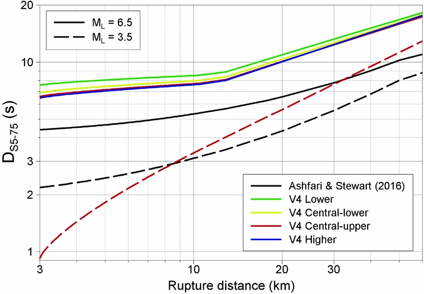
In each stage of development, the duration model from the previous stage was used to define the durations required for the stochastic simulations. At the V4 stage, this same procedure was followed, but now the limitation of the stochastic modelling approach was diminished because the durations are only input to the small-magnitude events – for which the duration model is constrained by the data from the field – representing patches of the fault rupture modelled in EXSIM. The durations from larger earthquakes are then obtained from the resulting time-histories generated at the NS_B horizon as a result of the interactions of the signals from the individual patches. Clearly the predicted durations therefore depend on the assumed rupture velocity and aspect ratio, but the basis for these estimates of the shaking duration are more physical than in previous models and consistent with the geophysical properties of the field. The durations predicted at the NS_B horizon are transformed to the ground surface via terms adapted from the Afshari & Stewart (Reference Afshari and Stewart2016a) model to match the local recordings; the site term is defined as a function of V S30, for which reason a map of median V S30 for each zone has been prepared (Bommer et al., Reference Bommer, Stafford, Edwards, Dost, van Dedem, Rodriguez-Marek, Kruiver, van Elk, Doornhof and Ntinalexis2017). Figure 11 compares predictions from the V4 duration model – in which there are four branches, each twinned with one of the branches for median spectral accelerations – with those from Afshari & Stewart (Reference Afshari and Stewart2016a). For small magnitudes – where all the V4 branches are equivalent – the V4 model captures the shorter durations close to the epicentre and the more rapid increase of duration with distance than modelled by the Afshari & Stewart (Reference Afshari and Stewart2016a) model, which is derived from recordings of tectonic earthquakes. For larger magnitudes, the predictions all show similar trends with distance, but the Groningen model yields durations almost twice as long as those from Afshari & Stewart (Reference Afshari and Stewart2016a). At this stage, it is not clear whether this is a genuine feature of motions from larger earthquakes in the gas field or simply the tendency for EXSIM to overestimate durations from empirical equations, as reported by Afshari & Stewart (Reference Afshari and Stewart2016b).
Predicted median durations as a function of distance from earthquakes of magnitude 3.5 and 6.5, using the four branches of the V4 model and the equation of Afshari & Stewart (Reference Afshari and Stewart2016a). For ML 3.5, all of the V4 branches are identical.
In applications to the risk modelling, the durations are predicted as conditional on the spectral accelerations using the correlation coefficients between residuals proposed by Bradley (Reference Bradley2011), which have been found to be generally consistent with the trends observed for Groningen motions.
Conclusion
A model for the estimation of ground-motion amplitudes and durations due to induced earthquakes in the Groningen field has been developed through an evolutionary process. The framework of the model is now stable in terms of prediction of motions at a reference rock horizon (the base of the North Sea Supergroup at 800m depth) using extended ruptures to represent earthquake sources, and convolution of these rock motions with nonlinear, frequency-dependent amplification factors to obtain the motions at the ground surface. The model is consistent with available data for the Groningen field but also captures the epistemic uncertainty associated with extrapolations for the larger earthquake scenarios considered in hazard and risk estimation. Work is ongoing to further refine the model, but future changes are now expected to be incremental. The V4 Groningen GMM can be used to estimate losses due to potential future earthquakes in the gas field and to define inputs to earthquake-resistant design of structures.
Acknowledgements
There are too many people who have contributed to this work to mention them all here, but in addition to those mentioned in the text a special note of thanks is due to some individuals with whom very constructive and helpful discussions have been held throughout the development of this work: at KNMI, Jesper Spetzler and Elmer Ruigrok, and those who together with the first author of this paper form the NAM seismic hazard and risk modelling team, namely Stephen Bourne, Helen Crowley, Steve Oates and Rui Pinho. We also wish to express our gratitude to John Douglas and an anonymous reviewer for helpful comments on the original version of this paper, and to guest editor Karin von Thienen-Visser for assistance with the processing of this contribution.


 Open access