


1 Introduction
Longitudinal mental health assessments in mobile health (mHealth) applications have been found to be a scalable and effective way to capture information on a user’s current mental health status (Pardes et al., Reference Pardes, Lynch, Miclette, McGeoch and Daly2022). Because these assessments may be performed many times over the course of months or years, researchers have the opportunity to model the trajectory of users’ mental health over time. For example, researchers may gain an understanding of changes in an mHealth user’s depressive symptoms over time by the regular completion of the Patient Health Questionnaire-4 (PHQ-4) (Löwe et al., Reference Löwe, Wahl, Rose, Spitzer, Glaesmer, Wingenfeld, Schneider and Brähler2010). While each assessment yields only a handful of item responses, the high-frequency sampling makes each individual’s longitudinal record intrinsically high-dimensional, and analysis thus focuses on recovering the underlying latent trajectory that generates the data.
Yet recovering these trajectories accurately demands proper handling of the measurement scale: most questionnaire items use Likert responses, which violate assumptions like normality and can bias standard models (Wu & Leung, Reference Wu and Leung2017). Ordinal regression addresses this by assuming a latent continuous variable that is mapped to observed categories via a link function and threshold values (McCullagh, Reference McCullagh1980).
Like ordinal regression, polytomous IRT models (Reeve & Fayers, Reference Reeve and Fayers2005) use continuous latent variables to quantify constructs from multi-category items. In particular, the graded response model (GRM) (Samejima, Reference Samejima1968) is tailored to ordered outcomes, such as Likert-scale responses. Specifically, in the typical GRM model,

where j represents a questionnaire item, k represents an ordered response,
$K_j$
 represents the maximum ordered response for item j,
$\theta $
represents the maximum ordered response for item j,
$\theta $
 represents the latent construct of interest, and
$P_{jk}(\cdot )$
represents the latent construct of interest, and
$P_{jk}(\cdot )$
 represents an inverse link function (Samejima, Reference Samejima1968). Additional parameters may also be included in the model to adjust for item difficulty and discrimination (Hays et al., Reference Hays, Morales and Reise2000). A special case of the GRM (Cole et al., Reference Cole, Turner and Gitchel2019) includes item difficulty parameters,
$\delta _j$
represents an inverse link function (Samejima, Reference Samejima1968). Additional parameters may also be included in the model to adjust for item difficulty and discrimination (Hays et al., Reference Hays, Morales and Reise2000). A special case of the GRM (Cole et al., Reference Cole, Turner and Gitchel2019) includes item difficulty parameters,
$\delta _j$
 , item discrimination parameters,
$a_j$
, item discrimination parameters,
$a_j$
 , and shared threshold parameters,
$\tau _{k}$
, and shared threshold parameters,
$\tau _{k}$
 , with a logistic link such that

This model assumes that the thresholds
$\tau _k$
 are constant across items, that is, that the scale is the same for different items, an assumption that has precedent in psychometric research where scales are the same across items (Lubbe & Schuster, Reference Lubbe and Schuster2019).
IRT models may be extended for use in longitudinal data by allowing
$\theta $
 to vary within subjects over time (Choi, Reference Choi2024; Proust-Lima et al., Reference Proust-Lima, Philipps, Perrot, Blanchin and Sébille2022; Wang & Nydick, Reference Wang and Nydick2020). For example, Liu and Hedeker (Reference Liu and Hedeker2006) used IRT and mixed-effects modeling techniques to model latent subject ability over time based on multi-item Likert-scale questionnaires. Random intercepts and slopes were included to account for variation between subjects and over time. While simple parametric approaches for analyzing longitudinal data, such as random time slopes, are useful in assessing the change in latent continuous variables overtime, they often lack flexibility or are misspecified to capture nonlinear trends in the data (Wang et al., Reference Wang, Chiou and Müller2016). Thus, it is often preferred to use nonparametric methods to model trajectories as a function of time, that is, perform functional data analysis (FDA) (Liu & Wang, Reference Liu and Wang2020; Wang et al., Reference Wang, Chiou and Müller2016).
Gaussian processes (GPs) are stochastic processes such that every finite collection of random variables has a multivariate Gaussian distribution (Liu et al., Reference Liu, Wang and Kong2019). GPs are specified by a covariance matrix that accounts for correlation between points and controls for smoothness, making them an attractive option for FDA (Shi & Choi, Reference Shi and Choi2011). Because of their correlation structure, they are useful for modeling trajectories in a variety of settings (Chen & Zhang, Reference Chen and Zhang2020; Kim et al., Reference Kim, Lee and Essa2011).
There is precedent for using GP regression in both ordinal data and IRT settings. For example, Komori et al. (Reference Komori, Teraji, Shiroshita and Nittono2022) used Bayesian ordinal GPR to determine which facial features in children are perceived as cute, where cuteness was measured on a scale of integer values from 1 to 5. Others have explored the use of power link functions in ordinal GPR (Li et al., Reference Li, Wang and Dey2019). Chen and Zhang (Reference Chen and Zhang2020) used a latent GP model to model longitudinal survey data in psychology applications, remarking how their approach is similar to IRT models. While their paper provides a foundation in using GPs for longitudinal surveys, they only demonstrated the use of the ordinal component of their model in a simple simulation setting, without the complexity of real-world data that may complicate computation and parameter estimation. Kang and Kottas (Reference Kang and Kottas2024) showed how GPs can be used to understand mental health trajectories derived from ecological momentary assessments (EMAs). However, their method requires analyzing different items separately. It also uses the continuation logits representation of the multinomial distribution, resulting in different latent curves for each consecutive category combination. The interpretation of these curves is less clear than a single curve representing the latent construct of interest.
While GPs are frequently used in a Bayesian setting, where model fit is usually performed using Markov chain Monte Carlo (MCMC) techniques to sample from the posterior distribution, sampling from the posterior distribution of GPs can be challenging, especially in the often high-dimensional setting of a longitudinal analysis (Riutort-Mayol et al., Reference Riutort-Mayol, Bürkner, Andersen, Solin and Vehtari2023). Many researchers, including Chen and Zhang (Reference Chen and Zhang2020), choose to use empirical Bayes to estimate these parameters. However, a fully Bayesian approach to fitting a GP model may be desired.
In addition to modeling individual-level trends using a GP, researchers may also be interested in population-level trajectories within an IRT model. This may be done by modeling the mean function of a GP in a hierarchical setting using parametric or nonparametric approaches (Chen & Zhang, Reference Chen and Zhang2020). While Chen and Zhang (Reference Chen and Zhang2020) mentioned the possibility of using nonparametric approaches for estimating the mean function of the GP prior placed on individual trajectories, in practice, they modeled the mean function of the GP using only simple linear regression, reducing the model’s flexibility in recovering overall trends.
Smoothing splines, which balance model fit and smoothness, are a popular FDA technique that can be useful for modeling the mean of a GP (Chen & Zhang, Reference Chen and Zhang2020; Rice & Rosenblatt, Reference Rice and Rosenblatt1983; Shi et al., Reference Shi, Wang, Murray-Smith and Titterington2007). Smoothing splines can generally be described as a set of piecewise polynomial equations joined together at points called knots (Wang, Reference Wang2011). B-splines are a type of spline that have been shown to have excellent numerical properties, are sparse (desirable in high-dimensional settings), and are flexible in the presence of equally spaced knots (De Boor, Reference De Boor1978; Eilers & Marx, Reference Eilers and Marx2010). Specifically, define q knots
$\boldsymbol {\xi }=\{\xi _1\leq \xi _2 \leq , \cdots \leq \xi _q\}$
 . Then the
$j^{th}$
. Then the
$j^{th}$
 B-spline of degree p evaluated at point x can be defined recursively as (Lyche et al., Reference Lyche, Manni and Speleers2018)

with

Smooth curves may be estimated as a weighted sum of realizations of basis functions that are evaluated at points along the domain. In terms of regression, these weights may be thought of as coefficients that need to be estimated. Shi et al. (Reference Shi, Wang, Murray-Smith and Titterington2007) showed that B-spline basis functions are an excellent choice for GP functional regression, where it is computationally efficient to estimate the coefficients associated with the basis functions. B-splines also have local support, which allows one part of a curve fit to be adjusted without causing undue adjustments to other parts of the curve (De Boor, Reference De Boor1978). In practice, the degree of
$p=3$
 is commonly chosen and is the default in many standard statistical packages, such as in the splines package in R (R Core Team, 2022). A drawback to splines is that they may be highly sensitive to the location of the spline knots, which can be difficult to choose or estimate (Yang et al., Reference Yang, Zhang and Zhang2023). Cross-validation and other model fit evaluation techniques may be used to make these decisions.
There are many challenges associated with GP ordinal regression. For example, without additional constraints, the ordinal regression problem is scale invariant. A common solution is to fix the variance associated with the GP and to model the correlation matrix. However, modeling correlation matrices is much more challenging than covariance matrices (DeYoreo & Kottas, Reference DeYoreo and Kottas2018). The ordering constraint in the threshold values,
$\boldsymbol {\tau }$
 , also results in highly correlated posterior draws. DeYoreo and Kottas (Reference DeYoreo and Kottas2018) used mixture modeling, which allows the threshold values to be fixed, reducing computational burdens. However, the interpretation of this mixture modeling in an IRT setting is not clear.
One option to improve computational efficiency is the use of low-rank approximations of GPs (Reeve & Fayers, Reference Reeve and Fayers2005). Solin and Särkkä (Reference Solin and Särkkä2020) proposed the use of Hilbert space methods for reduced-rank GP regression. Riutort-Mayol et al. (Reference Riutort-Mayol, Bürkner, Andersen, Solin and Vehtari2023) explored the practical use of this rank reduction technique and demonstrated that Hilbert basis functions can be used to adequately approximate GPs in practical settings when the number of basis functions is sufficiently large and an appropriate boundary factor is assumed. More specific details on the computational challenges associated with a GP IRT model will be discussed in Section 4.2 after the full model is specified for clarity. We will also provide more detail on the Hilbert approximation and how it improves computational speed and posterior draw mixing in Section 4.3.
This article contributes to the current literature by demonstrating how mental health trajectories can be modeled as a GP within a hierarchical IRT model using Hilbert approximations for computational efficiency. Specifically, we use a GRM with equal thresholds for each item and place a GP prior on the latent construct of interest for each individual over time. We also capture population-level trends over time via smoothing splines. We explore this modeling approach in the context of mHealth survey data on a Likert scale collected in an educational setting. Because mHealth data are high-dimensional, we approximate the posterior distribution of the latent mental health trajectory GP using Hilbert basis functions to facilitate computational efficiency while still obtaining reasonable parameter uncertainty estimates. The efficacy of this approach is demonstrated via simulation. We also discuss model inference in the context of a motivating example. While in this article we present the methodology under a GRM assumption, we emphasize that the methods can easily be extended to other IRT settings where ordinal data meant to capture the trajectory of a unidimensional latent construct are collected frequently over time.
The rest of the article is outlined as follows. In Section 2, we introduce our motivating example. In Section 3, we propose the ordinal GP model for health trajectories (GPMHT). In Section 4, we outline our methods for Bayesian inference, including the prior specification, challenges associated with sampling from the joint posterior, and the Hilbert space approximation of the joint posterior. In Section 5, we discuss our simulation study to show that our Bayesian sampling techniques converge adequately and recover the unknown parameters and trajectories. In Section 6, we present the results of our motivating example analysis and compare our model to a model fit without a GP prior. Finally, we offer a few conclusions in Section 7.
2 Motivating example: College Experience study
Researchers at Dartmouth University have been using mHealth applications to study student health and behavior for many years, and have made their data publicly available (Wang et al., Reference Wang, Chen, Chen, Li, Harari, Tignor, Zhou, Ben-Zeev and Campbell2017). The most recent study, known as the College Experience Study, follows over 200 students who enrolled as freshmen in 2017 or 2018 over the course of their four years at Dartmouth via the StudentLife app (Nepal et al., Reference Nepal, Liu, Pillai, Wang, Vojdanovski, Huckins, Rogers, Meyer and Campbell2024). We focus on the students’ freshman year for reasons discussed in Appendix A.
The College Experience data are comprised of sensing data and EMAs intended to capture students’ behavior and mental health. We wish to develop a model that can be used to understand student mental health trajectories based on EMA responses. Included in the EMA data are responses to the photographic affect meter (PAM) (Pollak, Reference Pollak2012), PHQ-4, and four questions from the State Self-Esteem Scale (SSES) (Heatherton & Polivy, Reference Heatherton and Polivy1991) to measure mood, depression, and self-esteem, respectively. Each of these measures was requested approximately weekly from students via the app, although response rates vary. Other information on the students was collected, such as location, audio, and movement. However, due to a large amount of missing data, we focus on developing a flexible modeling framework for the EMAs without covariates.
We chose to model the SSES data because they represent multi-item surveys where responses varied over time. To avoid overfitting, we only included the 191 students who completed the SSES at least 30 times over the course of the three terms. The SSES is generally issued as a 20-item questionnaire to assess performance, social, and appearance self-esteem. Responses are on a Likert scale with the following options: 1) not at all, 2) a little bit, 3) somewhat, 4) very much, and 5) extremely. In the College Experience study, only four items were administered: 1) Right now, I worry about what other people think of me, 2) Right now, I am pleased with my appearance, 3) Right now, I feel as smart as others, and 4) Right now, overall, I feel good about myself. Note that item one is reverse coded. However, it is assumed for the rest of the article that it has been recoded so that a 5 represents high self-esteem and a 1 represents low self-esteem.
Importantly, the GRM assumes that there is a unidimensional latent construct that is measured by each item on a questionnaire (Andrich, Reference Andrich1978), while the SSES was designed to measure multiple aspects of a person’s self-esteem. However, studies have found that while the SSES captures multiple aspects of self-esteem, the composite score can be used as an effective measure of general self-esteem consistent with other rating scales (Linton & Richard, Reference Linton and Richard1996; Webster et al., Reference Webster, Howell and Shepperd2022).
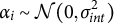
The concept of an overall self-esteem measure is supported by our exploratory data analysis. Figure 1 contains the average student response to the SSES items by day. We see that although the questions vary in “difficulty” (responses tend to be highest for item 1 and lowest for item 4), the trend in responses appears to be consistent across all items. Thus, we felt comfortable using the four SSES items to measure an overall self-esteem construct.
Average SSES responses by day and question over the course of the students’ freshman year.

Figure 1 Long description
The graph features a vertical y-axis labeled Response ranging from 2 to 5 and a horizontal x-axis labeled Day ranging from 0 to over 200. Four jagged line series represent different items.
* Item 1, shown in pink, maintains the highest average response, starting near 5, fluctuating between 3.5 and 4.5, and ending around 3.5.
* Item 4, shown in purple, generally sits below Item 1, fluctuating between 3 and 4 with a significant early peak near day 10.
* Item 2, in olive green, and Item 3, in light blue, are closely clustered at the bottom of the data set, frequently overlapping between the 2.5 and 3.5 response marks.
All four items show high daily volatility but follow a similar broad trend of a slight decline or stabilization after the initial 100 days.
While the trend in self-esteem appears clear in Figure 1, the trend is less obvious in the patterns of individual students. Figure 2 shows the responses of a random subset of eight students over the three terms. Due to the discrete nature of the scale, it is difficult to ascertain common patterns in self-esteem from these raw values. We show in this article how we can obtain smooth individual-level self-esteem trajectories for students that help us better picture trends in their mental health.
SSES responses by day, item, and student over the course of the students’ freshman year.

Figure 2 Long description
A multi-panel line graph titled S S E S Response by Day, Item, and Student I D. The Y-axis represents Response on a scale from 1 to 5. The X-axis represents Day from 0 to over 200. A legend on the right identifies four items by color: Item 1 is pink, Item 2 is olive green, Item 3 is light blue, and Item 4 is purple.
Eight panels are arranged in two rows of four, each labeled with a student I D:
* Top row: I D 12, I D 27, I D 36, and I D 96.
* Bottom row: I D 177, I D 182, I D 187, and I D 196.
Data trends across panels:
* I D 12: High density of responses starting from day 0, with frequent fluctuations between 2 and 5 across all items.
* I D 27: Responses begin around day 25, showing a downward trend for Item 1 and Item 4 toward the end of the period.
* I D 36: Sparse data points with Item 3 showing peaks at 4 and Item 2 dropping to 1 near day 250.
* I D 96: Data starts after day 50, with most items fluctuating between 2 and 4.
* I D 177: High volatility starting around day 50, with Item 1 and Item 3 reaching 5 and dropping to 1.
* I D 182: Responses clustered between days 75 and 250, with Item 2 showing a significant drop to 1 early on.
* I D 187: Item 1 maintains a high response of 5 for much of the early period, while other items fluctuate between 2 and 4.
* I D 196: Item 1 shows a sustained peak at 5 between days 50 and 100, while Item 2 has a sharp spike to 5 near day 200.
In general, we found that item 1 responses tend to be higher than the responses for items 2–4. We also found evidence that item discrimination may be lower for item 1 than the other items, as indicated by the decreased variation in responses. Please refer to a histogram of the data in Appendix B for additional support of these assertions (Figure B1).
The goals of the analysis of the College Experience study are as follows: 1) to understand how the self-esteem of all freshmen at Dartmouth changes over the course of their first year on campus and 2) quantify and visualize how individual students’ self-esteem trajectories differ from the average Dartmouth freshman population. Understanding general trends in self-esteem can guide the university in offering interventions to the general student body. By studying trends in individual students, officials may be able to identify students whose trajectories reveal concerning patterns that deviate from the average who might need extra support.
3 The proposed Gaussian process model for health trajectories
In this section, we introduce the GPMHT, describe it in the context of our motivating example, and discuss adjustments for other settings.
3.1 GPMHT
Let
$Y_{ijt}$
 represent subject i’s response to item j in a Likert scale questionnaire on day t. We assume that all responses can take on integer values
$1, \dots , K,$
represent subject i’s response to item j in a Likert scale questionnaire on day t. We assume that all responses can take on integer values
$1, \dots , K,$
 where
$K>2$
where
$K>2$
 . Let
$\delta _j$
. Let
$\delta _j$
 represent the “difficulty” of item j for
$j=1, \dots , J$
represent the “difficulty” of item j for
$j=1, \dots , J$
 and let
$\tau _0<\tau _1 < \tau _2 < \dots < \tau _{K-1}<\tau _K$
and let
$\tau _0<\tau _1 < \tau _2 < \dots < \tau _{K-1}<\tau _K$
 , where
$\tau _0=-\infty $
, where
$\tau _0=-\infty $
 and
$\tau _K=\infty $
and
$\tau _K=\infty $
 , represent threshold values that map values from the real numbers to the ordinal Likert scale. Let
$\theta _{i,t}$
, represent threshold values that map values from the real numbers to the ordinal Likert scale. Let
$\theta _{i,t}$
 represent the latent construct of interest, self-esteem in our motivating example, for subject i on day t. Then, we define


where
$\text {logit}^{-1}(\phi )=1/(1+e^{-\phi })$
 . This is a formulation of the GRM described in Equation (1.2). Thus, we assume that the items of the SSES measure a unidimensional construct, that the difference between two consecutive points on the scale is equal for all items, higher ratings represent higher values of the latent construct, and responses to items administered at the same time are conditionally independent of each other given the latent trait. We chose the logit link to relax the assumption of an underlying latent normal distribution implied by a probit link.
We now introduce a hierarchical component to the model to understand the trajectory of the latent construct
$\theta _{i,t}$
 . Assume that we have observations (item responses) recorded for subject i at
$T_i$
. Assume that we have observations (item responses) recorded for subject i at
$T_i$
 unique time points. Let
$\mathbf {t}_i=(t_{i,1}, \dots , t_{i, T_i})'$
unique time points. Let
$\mathbf {t}_i=(t_{i,1}, \dots , t_{i, T_i})'$
 represent a
$T_i \times 1$
represent a
$T_i \times 1$
 vector of observed days/time points for subject i. We consider
$\boldsymbol {\theta }_i=(\theta _{i,t_{i,1}}, \dots , \theta _{i,t_{i,T_i}})'$
vector of observed days/time points for subject i. We consider
$\boldsymbol {\theta }_i=(\theta _{i,t_{i,1}}, \dots , \theta _{i,t_{i,T_i}})'$
 to be realizations from a function of
$\mathbf {t}_i$
to be realizations from a function of
$\mathbf {t}_i$
 such that
$\boldsymbol {\theta }_i=f(\mathbf {t}_i)$
such that
$\boldsymbol {\theta }_i=f(\mathbf {t}_i)$
 . Let
$t_{i,r}$
. Let
$t_{i,r}$
 and
$t_{i,s}$
and
$t_{i,s}$
 represent the
$r^{th}$
represent the
$r^{th}$
 and
$s^{th}$
and
$s^{th}$
 elements of
$\mathbf {t}_i$
elements of
$\mathbf {t}_i$
 , respectively. Then we assume that this function follows a GP prior (Shi & Choi, Reference Shi and Choi2011) with a squared exponential kernel such that

where
$\boldsymbol {\mu }(\mathbf {t}_i)$
 is a
$T_i \times 1$
is a
$T_i \times 1$
 vector representing the mean function and
$\boldsymbol {\psi }$
vector representing the mean function and
$\boldsymbol {\psi }$
 is a
$T_i \times T_i$
is a
$T_i \times T_i$
 matrix where the element in the
$r^{th}$
matrix where the element in the
$r^{th}$
 row and
$s^{th}$
row and
$s^{th}$
 column equals
$\psi (t_{i,r}, t_{i,s})$
column equals
$\psi (t_{i,r}, t_{i,s})$
 . Further,
$\ell $
. Further,
$\ell $
 represents the lengthscale of the kernel, determining the smoothness of the GP. We chose to use the squared exponential kernel because it is a simple kernel function that depends only on the distance between points (regardless of direction) while ensuring smoothness. Other kernels could be explored if desired. Specifically, a Matérn kernel (
$\nu =3/2$
represents the lengthscale of the kernel, determining the smoothness of the GP. We chose to use the squared exponential kernel because it is a simple kernel function that depends only on the distance between points (regardless of direction) while ensuring smoothness. Other kernels could be explored if desired. Specifically, a Matérn kernel (
$\nu =3/2$
 or
$5/2$
or
$5/2$
 ) could be used for rougher sample paths, rational–quadratic for multi-scale variation, or periodic components if seasonality is desired. Given the ordinal likelihood and our sampling resolution, differences among these kernels primarily affect high-frequency roughness of
$g_i(\mathbf {t}_i)=\boldsymbol {\theta }_i-\mu (\mathbf {t}_i)$
) could be used for rougher sample paths, rational–quadratic for multi-scale variation, or periodic components if seasonality is desired. Given the ordinal likelihood and our sampling resolution, differences among these kernels primarily affect high-frequency roughness of
$g_i(\mathbf {t}_i)=\boldsymbol {\theta }_i-\mu (\mathbf {t}_i)$
 , which is weakly identified relative to the low-frequency mean
$\mu (\mathbf {t}_i)$
, which is weakly identified relative to the low-frequency mean
$\mu (\mathbf {t}_i)$
 . For this reason—and to keep the manuscript focused—we retain the SE kernel in the main analysis and note kernel exploration as a natural extension for future work.
While
$\boldsymbol {\theta }_i$
 represents smooth individual trajectories at the individual level, we also want to collect information on the average trajectory at the population level. We do this using cubic B-splines with D degrees of freedom (this corresponds to D-3 interior knots). Specifically, we set

where
$\boldsymbol {B}_{\mu }(t)$
 corresponds to a
$D \times 1$
corresponds to a
$D \times 1$
 vector of B-spline basis functions evaluated at t, and
$\boldsymbol {\beta }$
vector of B-spline basis functions evaluated at t, and
$\boldsymbol {\beta }$
 is a
$D\times 1$
is a
$D\times 1$
 vector of coefficients. We place the knots equally across the days of the study. A higher value of D corresponds to a more flexible curve, but can also be prone to overfit if the curve becomes too wiggly. In practice, we chose the value of D by comparing cross-validation results under different values, as will be discussed in Section 6.2.
There are several constraints required to ensure identifiability of the GRM in Equation (3.2). Because
$Y_{ij}$
 depends on
$\theta _{i,t}$
depends on
$\theta _{i,t}$
 and the cutpoints only through
$a_j\{\theta _{i,t}-(\delta _j+\tau _k)\}$
and the cutpoints only through
$a_j\{\theta _{i,t}-(\delta _j+\tau _k)\}$
 , the likelihood is invariant to location and scale transformations. We therefore adopt the following conventions. First, to fix the location, we omit an intercept from
$\boldsymbol {\mu }(x)$
, the likelihood is invariant to location and scale transformations. We therefore adopt the following conventions. First, to fix the location, we omit an intercept from
$\boldsymbol {\mu }(x)$
 . With
$\{\tau _k\}$
. With
$\{\tau _k\}$
 ordered, this determines the decomposition between latent traits, item locations, and step offsets. Second, we take the GP prior in Equation (3.3) to have unit marginal variance.
While we have formulated this model as a GRM with equal thresholds, Equations (3.1) and (3.2) can be adjusted for other settings. Specifically, a different link function may be used in (3.1) while still maintaining the ordinal nature of the data. In Equation (3.2), one may wish to assume different scales for each item by incorporating different thresholds
$\tau _{j,k}$
 . These adjustments may be easily made, although, care should be taken to ensure parameter identifiability.
4 Bayesian inference on the posterior
Because of the complexity of the model outlined in Section 3.1, we turned to Bayesian methods for inference. In this section, we first introduce our prior specification. We then explain the challenges associated with sampling from the joint posterior and describe the Hilbert space approximation as a potential solution.
4.1 Prior specification
We selected fairly noninformative priors for our unknown parameters, reflecting our lack of prior information. Specifically, we assumed that
$\ell \sim \mathcal {LN}(0,0.5)$
 , where
$\mathcal {LN}$
, where
$\mathcal {LN}$
 represents the log-normal distribution. We assumed that
$\tau _1, \dots , \tau _4$
represents the log-normal distribution. We assumed that
$\tau _1, \dots , \tau _4$
 each were normally distributed with mean zero and variance four under the constraint that
$\tau _1<\tau _2< \dots <\tau _{K-1}$
each were normally distributed with mean zero and variance four under the constraint that
$\tau _1<\tau _2< \dots <\tau _{K-1}$
 . We then assumed
$a_j^* \sim \mathcal {LN}(0, 0.5)$
. We then assumed
$a_j^* \sim \mathcal {LN}(0, 0.5)$
 such that
$a_j=a^*_j/(1/J\sum _{j=1}^Ja^*_j)$
such that
$a_j=a^*_j/(1/J\sum _{j=1}^Ja^*_j)$
 . Next, we let
$\delta ^*_j \sim \mathcal {N}(0, 1)$
. Next, we let
$\delta ^*_j \sim \mathcal {N}(0, 1)$
 and
$\delta _j=\delta ^*_j-1/J\sum _{i=1}^J\delta _j^*$
and
$\delta _j=\delta ^*_j-1/J\sum _{i=1}^J\delta _j^*$
 , where
$\mathcal {N}$
, where
$\mathcal {N}$
 represents the normal distribution. Note that the sum-to-zero constraint on
$\delta _j$
represents the normal distribution. Note that the sum-to-zero constraint on
$\delta _j$
 and the multiply-to-one constraint on
$a_j$
and the multiply-to-one constraint on
$a_j$
 are not strictly necessary for identifiability. However, in our setting, we found them helpful to speed convergence, with minimal impact on the interpretation of the latent long-term trends. Since we only have four items for analysis, identifying a complex latent structure over time may be difficult (Akour & AL-Omari, Reference Akour and AL-Omari2024). Other authors have discussed this issue, including Fox (Reference Fox2010) who notes that it can be challenging to identify a complex IRT model by fixing parameters of a prior, and these additional constraints may be helpful. In practice, the combination of weakly informative priors and constraints mainly aids convergence when relatively few items or observations are available. As more intensive mHealth data accumulate, the likelihood will dominate the weakly informative priors, and fewer constraints may be applied. Finally, we assumed
$\beta _d \sim \mathcal {N}(0, \sigma ^2)$
are not strictly necessary for identifiability. However, in our setting, we found them helpful to speed convergence, with minimal impact on the interpretation of the latent long-term trends. Since we only have four items for analysis, identifying a complex latent structure over time may be difficult (Akour & AL-Omari, Reference Akour and AL-Omari2024). Other authors have discussed this issue, including Fox (Reference Fox2010) who notes that it can be challenging to identify a complex IRT model by fixing parameters of a prior, and these additional constraints may be helpful. In practice, the combination of weakly informative priors and constraints mainly aids convergence when relatively few items or observations are available. As more intensive mHealth data accumulate, the likelihood will dominate the weakly informative priors, and fewer constraints may be applied. Finally, we assumed
$\beta _d \sim \mathcal {N}(0, \sigma ^2)$
 for
$d=1, \dots , D$
for
$d=1, \dots , D$
 . We then set
$\sigma \sim \mathcal {C}(0,1),$
. We then set
$\sigma \sim \mathcal {C}(0,1),$
 where
$\mathcal {C}$
where
$\mathcal {C}$
 represents the Cauchy distribution. In this way, we established a random effects interpretation for fitting the splines, and the spline coefficients are centered at zero. One can interpret this prior as a Bayesian equivalent to ridge regression, so that the spline coefficients are drawn toward zero (James et al., Reference James, Witten, Hastie and Tibshirani2013). A discussion of the full likelihood and joint posterior distribution can be found in Appendices C and D, respectively.
4.2 Challenges with sampling from full joint posterior distribution
Because of the complexity of the joint posterior distribution induced by the GPMHT likelihood and its prior specification, its closed form is not readily available. Thus, we have to rely on MCMC techniques to sample from the posterior, which is a computationally expensive task. Note that MCMC methods sampling from the exact joint posterior require inverting the
$n\times n$
 covariance matrix of the latent GP at each update, an
$\mathcal {O}(n^3)$
covariance matrix of the latent GP at each update, an
$\mathcal {O}(n^3)$
 operation (Riutort-Mayol et al., Reference Riutort-Mayol, Bürkner, Andersen, Solin and Vehtari2023). In intensive longitudinal designs, where n grows with both the number of participants and repeated measurements, performing these inversions at every iteration becomes computationally prohibitive (Gu et al., Reference Gu, Wang and Berger2018).
Even aside from the
$\mathcal {O}(n^3)$
 cost of repeatedly inverting GP covariance matrices, Gibbs sampling (Gelfand, Reference Gelfand2000)—though appealing when full conditionals are available in closed form—introduces additional difficulties. Recall that

where
$\phi ^*_{i,j,t}=a_j(\theta _{i,t}-\delta _j)+\epsilon _{i,j,t}$
 ,
$\epsilon _{i,j,t}\sim \mathrm {Logistic}(0,1)$
,
$\epsilon _{i,j,t}\sim \mathrm {Logistic}(0,1)$
 and refer to Appendix E for details. Under this threshold formulation, the full conditional of
$\phi ^*_{i,j,t}$
and refer to Appendix E for details. Under this threshold formulation, the full conditional of
$\phi ^*_{i,j,t}$
 is truncated into the region
$[\tau _{k-1},\tau _k]$
is truncated into the region
$[\tau _{k-1},\tau _k]$
 when
$Y_{i,j,t}=k$
when
$Y_{i,j,t}=k$
 . When
$a_j(\theta _{i,t}-\delta _j)$
. When
$a_j(\theta _{i,t}-\delta _j)$
 lies far from this interval, draws would concentrate in extreme tails, causing numerical instability and poor mixing. In addition, the ordered cut-off points
$\tau _1<\cdots <\tau _{K-1}$
lies far from this interval, draws would concentrate in extreme tails, causing numerical instability and poor mixing. In addition, the ordered cut-off points
$\tau _1<\cdots <\tau _{K-1}$
 mix slowly, since their moves must respect both the order constraint and the current values of
$\boldsymbol {\phi }^{*}=\{\phi _{i,j,t}^*\}$
mix slowly, since their moves must respect both the order constraint and the current values of
$\boldsymbol {\phi }^{*}=\{\phi _{i,j,t}^*\}$
 and
$\mathbf {Y}=\{Y_{i,j,t}\}$
and
$\mathbf {Y}=\{Y_{i,j,t}\}$
 . These couplings among
$\theta _{i,t}$
. These couplings among
$\theta _{i,t}$
 ,
$\delta _j, a_j$
,
$\delta _j, a_j$
 , and
$\boldsymbol {\tau }$
, and
$\boldsymbol {\tau }$
 are amplified further in high-dimensional longitudinal data, yielding highly autocorrelated chains even with long runs.
We have attempted to fit the GP ordinal regression model using an MCMC sampler with a probit link for computational simplicity. In applied analyses, the strong posterior dependence between the cut-off points and the latent trajectories led to poor mixing and inadequate exploration of the parameter space; even for long runs, standard convergence diagnostics did not indicate convergence. Increasing the number of iterations was impractical due to the cubic cost of repeated GP covariance matrix inversions at each iteration.
We further explored methods outside of Gibbs sampling, including the use of Rstan or Stan (Stan Development Team, 2024). Stan performs MCMC using the No U-Turn Sampler (NUTS) version of Hamiltonian Monte Carlo to facilitate efficient sampling from the posterior (Hoffman & Gelman, Reference Hoffman and Gelman2014). While NUTS is efficient in many regards, its computation times can still be high, especially when estimating continuous functions like a GP and in the case of high-dimensional data, such as the College Experience study (Stan Development Team, 2024). In practice, applying NUTS to the exact joint posterior did not achieve convergence after seven days of computation, primarily because each iteration requires repeated Cholesky factorizations of large GP covariance matrices. We therefore adopted a Hilbert-space GP approximation to reduce computational burden and enable tractable sampling.
4.3 Hilbert approximation for GPs
We give a brief description of the Hilbert approximation for GPs. For more detailed explanations and derivations, one should see Riutort-Mayol et al. (Reference Riutort-Mayol, Bürkner, Andersen, Solin and Vehtari2023). It can be shown that stationary covariance functions may be represented by their spectral densities (Riutort-Mayol et al., Reference Riutort-Mayol, Bürkner, Andersen, Solin and Vehtari2023). The squared-exponential kernel spectral density is defined as

Next, we can define a domain,
$\Omega $
 , such that for some positive value, L,
$\Omega \in [-L, L]$
, such that for some positive value, L,
$\Omega \in [-L, L]$
 . Let
$\lambda _q$
. Let
$\lambda _q$
 and
$\{\phi _q(x)\}_{q=1}^{\infty }$
and
$\{\phi _q(x)\}_{q=1}^{\infty }$
 represent the eigenvalues and eigenvectors, respectively, of the Laplacian operator with respect to the domain
$\Omega $
represent the eigenvalues and eigenvectors, respectively, of the Laplacian operator with respect to the domain
$\Omega $
 . Then, for sufficiently large m,

where
$\boldsymbol {\phi }(t)=\{\phi _q(t)\}_{q=1}^m \in \mathbb {R}^m$
 is the column vector of basis functions and
$\boldsymbol {\Delta }\in \mathbb {R}^{m\times m}$
is the column vector of basis functions and
$\boldsymbol {\Delta }\in \mathbb {R}^{m\times m}$
 is a diagonal matrix of
$S(\sqrt {\lambda _q})$
is a diagonal matrix of
$S(\sqrt {\lambda _q})$
 for
$q=1, \dots , m$
for
$q=1, \dots , m$
 . Let
$\boldsymbol {\Phi }_i$
. Let
$\boldsymbol {\Phi }_i$
 be the
$T_i\times m$
be the
$T_i\times m$
 matrix of eigenfunctions. Then we can write

where
$\boldsymbol {\mu }_i$
 is the
$T_i \times 1$
is the
$T_i \times 1$
 mean vector evaluated at times
$t_{i,1}, \dots , t_{i, T_i}$
mean vector evaluated at times
$t_{i,1}, \dots , t_{i, T_i}$
 . If the mean is assumed to be zero, by properties of the multivariate normal distribution,

where
$\eta _q \sim \mathcal {N}(0,1)$
 . Assuming that the inputs
$|t|$
. Assuming that the inputs
$|t|$
 are sufficiently small enough to be in
$\Omega $
are sufficiently small enough to be in
$\Omega $
 and m is sufficiently large, then this is an appropriate approximation for the density of a GP. This can easily be adjusted for the case of a nonzero mean, since the mean can just be added to the GP realization.
In general, this approximation is more efficient than sampling from an exact GP because it reframes the problem into a linear model with coefficients
$\eta _1, \dots , \eta _m$
 . It also avoids the inversion of the covariance function (Riutort-Mayol et al., Reference Riutort-Mayol, Bürkner, Andersen, Solin and Vehtari2023). While the initial computational cost of calculating the basis functions is
$\mathcal {O}(m^2n)$
. It also avoids the inversion of the covariance function (Riutort-Mayol et al., Reference Riutort-Mayol, Bürkner, Andersen, Solin and Vehtari2023). While the initial computational cost of calculating the basis functions is
$\mathcal {O}(m^2n)$
 , the computational cost at each iteration of the sampler is only
$\mathcal {O}(mn+m)$
, the computational cost at each iteration of the sampler is only
$\mathcal {O}(mn+m)$
 . With
$m<<n$
. With
$m<<n$
 , this results in a significant computational advantage in high-dimensional settings when compared to samplers that require the inversion of the covariance function, which has a computational cost of
$\mathcal {O}(n^3)$
, this results in a significant computational advantage in high-dimensional settings when compared to samplers that require the inversion of the covariance function, which has a computational cost of
$\mathcal {O}(n^3)$
 .
.
Of course, the approximation in Equation (4.5) relies on the values of L and m. We followed the suggested methodology in Riutort-Mayol et al. (Reference Riutort-Mayol, Bürkner, Andersen, Solin and Vehtari2023) to tune these hyperparameters, as described in more detail in Appendix F. As part of the tuning, we also used context-specific metrics to assess whether L and m were sufficiently large such that larger values would not lead to significantly different results. Specifically, we calculated the within sample posterior predictive mean absolute deviation for items 1–4 (
$MAD_1$
 –
$MAD_4$
–
$MAD_4$
 ), which takes on values between 0 and 4, to assess convergence of the algorithm. To calculate this, assume we have R samples from the joint posterior distribution for each parameter. Let
$\hat {y}_{i,j,t}^{(r)}$
), which takes on values between 0 and 4, to assess convergence of the algorithm. To calculate this, assume we have R samples from the joint posterior distribution for each parameter. Let
$\hat {y}_{i,j,t}^{(r)}$
 represent the
$r^{th}$
represent the
$r^{th}$
 predicted value for
$y_{i,j,t}$
predicted value for
$y_{i,j,t}$
 . This is found by sampling from the model in Equations (3.1) and (3.2), where
$a_j$
. This is found by sampling from the model in Equations (3.1) and (3.2), where
$a_j$
 ,
$\theta _{i,t}$
,
$\theta _{i,t}$
 ,
$\delta _j$
,
$\delta _j$
 , and
$\tau _1, \dots , \tau _{K-1}$
, and
$\tau _1, \dots , \tau _{K-1}$
 are replaced by their
$r^{th}$
are replaced by their
$r^{th}$
 draw from the joint posterior distribution. We can then calculate

where
$|\mathbf {t}_i|$
 represents the cardinality of
$\mathbf {t}_i$
represents the cardinality of
$\mathbf {t}_i$
 . For each observation, we used
$R=6,000$
. For each observation, we used
$R=6,000$
 samples from the posterior to calculate this metric. We also used the predicted values to calculate the accuracy of the model for each item. We refer to these values as
$Acc_1$
samples from the posterior to calculate this metric. We also used the predicted values to calculate the accuracy of the model for each item. We refer to these values as
$Acc_1$
 –
$Acc_4$
–
$Acc_4$
 . The accuracy metric penalizes all incorrect predictions equally, discarding the importance of ordinality in the model.
Each time the model was fit, we sampled from the posterior using four chains with 3,000 samples each. A burn-in of 1,500 was used for each chain. We used four chains to ensure that chains converged to similar values regardless of starting point. Because we used multiple chains in our sampling procedure, we assessed the between and within chain variability of our parameter estimates using
$\hat {R}$
 , where values close to one indicate that the chains have converged adequately (Vehtari et al., Reference Vehtari, Gelman, Simpson, Carpenter and Bürkner2021). We also found the bulk effective sample size (ESS) (Vehtari et al., Reference Vehtari, Gelman, Simpson, Carpenter and Bürkner2021) for each parameter to assess the movement within chains. It is recommended that each parameter have an
$\hat {R}$
, where values close to one indicate that the chains have converged adequately (Vehtari et al., Reference Vehtari, Gelman, Simpson, Carpenter and Bürkner2021). We also found the bulk effective sample size (ESS) (Vehtari et al., Reference Vehtari, Gelman, Simpson, Carpenter and Bürkner2021) for each parameter to assess the movement within chains. It is recommended that each parameter have an
$\hat {R}$
 value less than 1.01, and a sufficiently large ESS (at least 100 per chain) (Stan Development Team, 2024). We found 3,000 draws from the posterior gave us ample room to meet these convergence standards. Sampling was done on 4 cores using around 30 GB of RAM for 191 subjects and 272 possible observed time points. Each fitting took around 6 hours. Note that, in the following sections, we will provide diagnostics and simulations that support the efficacy of our sampling algorithm. The Stan code is available in Appendix L.
In addition to tuning the Hilbert approximation, the number of splines used for the mean function must be tuned. We did this by comparing the within-sample predictive accuracy and mean absolute deviation measures discussed before for several different numbers of knots. We also compared cross-validation predictive accuracy measures to decide. We do not go into great detail here since spline tuning is well-studied, but the process for the College Experience study will be described in Section 6.2.
5 Simulation study
In order to assess whether samples from our MCMC algorithm adequately approximate the joint posterior distribution and recover unknown parameters and latent trajectories, we performed multiple simulation studies in this section.
5.1 Simulation for parameter recovery
To perform the simulation study for parameter recovery, we simulated
$M=100$
 data sets. These data were designed to emulate the data observed in the College Experience study by using the same structure of missingness and parameter values derived from the College Experience study. The procedure for generating each data set is described in Appendix G. After creating a simulated data set, we then used
$\texttt {Rstan}$
data sets. These data were designed to emulate the data observed in the College Experience study by using the same structure of missingness and parameter values derived from the College Experience study. The procedure for generating each data set is described in Appendix G. After creating a simulated data set, we then used
$\texttt {Rstan}$
 to sample from the joint posterior. For the simulation, we used four chains with 2,000 samples each. For each chain, we used a burn-in of 1,000. We decreased the number of draws from the main analysis to reduce computation time for the simulations. For the Hilbert approximation used
$c=2.271$
to sample from the joint posterior. For the simulation, we used four chains with 2,000 samples each. For each chain, we used a burn-in of 1,000. We decreased the number of draws from the main analysis to reduce computation time for the simulations. For the Hilbert approximation used
$c=2.271$
 and
$m=21$
and
$m=21$
 to match the values, we found to be adequate for the College Experience data.
5.1.1 Parameter recovery results
To assess parameter recovery, uncertainty, and convergence, we calculated several diagnostics for each of the parameters and 100 simulated data sets. Specifically, we found the bias, mean squared error (MSE), standard error (SE), standard deviation (SD), and coverage probability (CP) of the 95% credible intervals (CIs) for each parameter. Formulas for these metrics can be found in Appendix H. We also reported the average
$\hat {R}$
 and ESS value for each parameter across all 100 data sets. All of the diagnostics mentioned in this section for the simulation study are shown in Table 1.
Simulation diagnostics based on 100 simulated data sets for each parameter

Table 1 Long description
The table consists of 9 columns: Parameter, Value, Bias, S D, S E, M S E, C P, R-hat, and E S S.
* Row 1: Parameter ell, Value 1.226, Bias minus 0.002, S D 0.049, S E 0.049, M S E 0.002, C P 0.960, R-hat 1.003, E S S 922.840.
* Row 2: Parameter tau sub 1, Value minus 4.128, Bias 0.013, S D 0.121, S E 0.108, M S E 0.012, C P 0.950, R-hat 1.006, E S S 594.203.
* Row 3: Parameter tau sub 2, Value minus 2.003, Bias 0.011, S D 0.117, S E 0.102, M S E 0.010, C P 0.980, R-hat 1.007, E S S 569.291.
* Row 4: Parameter tau sub 3, Value 0.353, Bias 0.009, S D 0.117, S E 0.101, M S E 0.010, C P 0.970, R-hat 1.007, E S S 563.823.
* Row 5: Parameter tau sub 4, Value 2.733, Bias 0.012, S D 0.118, S E 0.102, M S E 0.010, C P 0.980, R-hat 1.006, E S S 578.110.
* Row 6: Parameter delta sub 1, Value minus 1.568, Bias minus 0.001, S D 0.039, S E 0.034, M S E 0.001, C P 0.990, R-hat 1.002, E S S 1,261.948.
* Row 7: Parameter delta sub 2, Value 0.710, Bias minus 0.001, S D 0.025, S E 0.022, M S E 0.000, C P 0.960, R-hat 1.002, E S S 1,298.820.
* Row 8: Parameter delta sub 3, Value 0.582, Bias 0.003, S D 0.022, S E 0.019, M S E 0.000, C P 0.970, R-hat 1.001, E S S 3,897.719.
* Row 9: Parameter delta sub 4, Value 0.276, Bias 0.000, S D 0.022, S E 0.021, M S E 0.000, C P 0.940, R-hat 1.001, E S S 2,098.532.
* Row 10: Parameter a sub 1, Value 0.809, Bias 0.002, S D 0.018, S E 0.019, M S E 0.000, C P 0.930, R-hat 1.001, E S S 4,073.811.
* Row 11: Parameter a sub 2, Value 1.133, Bias 0.001, S D 0.017, S E 0.018, M S E 0.000, C P 0.930, R-hat 1.001, E S S 4,010.251.
* Row 12: Parameter a sub 3, Value 0.989, Bias minus 0.002, S D 0.017, S E 0.017, M S E 0.000, C P 0.930, R-hat 1.001, E S S 4,018.790.
* Row 13: Parameter a sub 4, Value 1.068, Bias minus 0.001, S D 0.017, S E 0.016, M S E 0.000, C P 0.970, R-hat 1.001, E S S 3,993.396.
* Row 14: Parameter sigma, Value 0.431, Bias minus 0.004, S D 0.094, S E 0.092, M S E 0.008, C P 0.950, R-hat 1.001, E S S 3,590.733.
We found that each of the parameters exhibits a bias close to zero. Further, the SE and MSE values were close to zero for all parameters. The reported SD values for the cutoffs,
$\tau _1, \dots , \tau _4$
 , were somewhat high, possibly due to the high correlation in the parameters. However, the CPs for the 95% CIs were all at least 95% for these parameters. The CP for
$\ell $
, were somewhat high, possibly due to the high correlation in the parameters. However, the CPs for the 95% CIs were all at least 95% for these parameters. The CP for
$\ell $
 was 96%, suggesting that our Hilbert approximation is working appropriately. All parameters had a 95% CI CP of at least 93%, well within the range of reasonable values when only 100 data sets are simulated. We also found average
$\hat {R}$
was 96%, suggesting that our Hilbert approximation is working appropriately. All parameters had a 95% CI CP of at least 93%, well within the range of reasonable values when only 100 data sets are simulated. We also found average
$\hat {R}$
 values less than 1.01, suggesting the convergence of the chains. The average ESS was also reasonably large, averaging at least 100 samples per chain, for all parameters.
5.2 Simulation for trajectory recovery
Next, we simulated data to assess the model’s ability to recover individual mental health trajectories, with
$\boldsymbol {\theta }_i$
 defined as the sum of a population-level mean function (Equation (3.5)) and a subject-specific, zero-mean GP with covariance
$\boldsymbol {\psi }(\mathbf {t}, \mathbf {t}')$
defined as the sum of a population-level mean function (Equation (3.5)) and a subject-specific, zero-mean GP with covariance
$\boldsymbol {\psi }(\mathbf {t}, \mathbf {t}')$
 (Equation (3.4)). Focusing on the Hilbert approximation to the GP, we evaluated recovery of individual deviations,
$g_i(\mathbf {t}_i)=\boldsymbol {\theta }_i - \boldsymbol {\mu }(\mathbf {t}_i)$
(Equation (3.4)). Focusing on the Hilbert approximation to the GP, we evaluated recovery of individual deviations,
$g_i(\mathbf {t}_i)=\boldsymbol {\theta }_i - \boldsymbol {\mu }(\mathbf {t}_i)$
 , across scenarios using a single simulated dataset per setting to reflect practical conditions.
First, let us consider a scenario where the data are generated as in Section 5.1. However, we drew the mean function from a multivariate normal distribution with mean vector
$\mathbf {0}$
 , a correlation matrix given by a squared exponential kernel with lengthscale 0.5, and SD 0.5. By generating the data from a multivariate normal distribution with an infinitely differentiable covariance function, we are able to see whether splines, which have a finite number of knots, can adequately approximate a smooth mean function in this setting. We chose a lengthscale of 0.5 because we wanted to evaluate trajectory recovery under the scenario where the true underlying function is moderately wiggly. After fitting the model to the generated data, we then compared plots of the individual deviations from the mean function to the true deviations in the simulated data. The results for eight randomly selected trajectories are shown in Figure 3. The black lines indicate the true trajectory while the blue lines represent the median of the posterior distribution. Note that some of the black lines (true trajectory) are shorter than the blue lines (estimated trajectory) because in the College Experience study different students entered and left the study at different points in the year. As described in Section 5.1 and Appendix G, the data were generated to mimic this entry and exit pattern. Since our goal was to model the trajectory over the course of the entire freshman year, we felt it was useful to see the trajectory estimates (and uncertainty) associated with time points outside of a subject’s study period. This led to the blue and black curves displaying different lengths. We see that in most scenarios, the algorithm does an excellent job at capturing individual deviations from the mean for periods where data are available. For most parts of the curve, the true trajectory lies within the 95% CI bounds. We also see how the GP is useful in flexibly capturing a variety of different shapes in individual deviations from the mean function. Importantly, the uncertainty associated with our trajectory estimates is much greater during periods where data are unavailable (i.e., late entry or early exit) when compared to periods where data are available. To see how well the splines capture the mean trend, please see Appendix I.1. Note that the smooth mean function in the generated data was approximated well by the spline mean function with 16 degrees of freedom.
A comparison of simulated trajectories (black curves) to the estimated trajectories (as determined by the median of the posterior distribution, in blue). The shaded region represents 95% CI bounds. The data were designed to match the College Experience study. Thus, the black curves may be shorter than the blue curves to mimic late entry or early exit in the study. The full estimated curve is shown in blue since we want to make inference on the entire freshman year.

Figure 3 Long description
A multi-panel line graph titled Individual Deviation from Average. The x-axis is labeled Day, ranging from 0 to over 200. The y-axis is labeled Deviation from Average, ranging from negative 2 to 2. The figure contains eight panels arranged in two rows of four, labeled with participant numbers 14, 76, 85, 102, 111, 118, 148, and 159.
Each panel displays three data elements:
1. True Value: A solid black curve representing simulated data. These curves often start later or end earlier than the full time range.
2. Estimated: A solid blue curve representing the median posterior distribution, spanning the full x-axis.
3. 95% C I: A light blue shaded region surrounding the blue estimated curve.
Data trends by panel:
* Panel 14: Both curves show a U-shaped dip, bottoming out around day 150.
* Panel 76: The black curve starts late at day 100 and rises sharply, while the blue curve shows a gradual upward slope.
* Panel 85: Both curves show an inverted U-shape, peaking near day 150.
* Panel 102: Both curves show a slight sinusoidal wave, remaining relatively flat near 1.
* Panel 111: Both curves show an inverted U-shape peaking early near day 100.
* Panel 118: Both curves show a steady linear increase from negative 1 toward 0.
* Panel 148: Both curves show a downward asymptotic curve, leveling off near negative 2.
* Panel 159: Both curves show a shallow U-shaped dip, centered around day 150.
Many other simulations were performed to assess individual trajectory recovery under different values of
$\ell $
 , different numbers of items, and different numbers of possible ordinal responses. For brevity, the results of a select number of these simulations are in Appendix I. In general, we found that the model appropriately captures individual deviations from trajectories, even in challenging situations, including small values of
$\ell $
, different numbers of items, and different numbers of possible ordinal responses. For brevity, the results of a select number of these simulations are in Appendix I. In general, we found that the model appropriately captures individual deviations from trajectories, even in challenging situations, including small values of
$\ell $
 and low numbers of possible ordinal responses.
5.3 Simulation for comparison to baseline model
We also performed a simulation to compare model fit and trajectory recovery between our model and a baseline model without GP trajectories. Specifically, we defined the baseline model using Equations (3.1) and (3.2). However, we assumed
$\theta _{i,t}=\mu (t)+\alpha _i$
 , where
$\alpha $
, where
$\alpha $
 is a random intercept such that
$\alpha _i \sim \mathcal {N}(0, \sigma ^2_{int})$
is a random intercept such that
$\alpha _i \sim \mathcal {N}(0, \sigma ^2_{int})$
 and
$\mu (t)$
and
$\mu (t)$
 is defined as in Equation (3.5). To be consistent with the GPMHT, we used 16 degrees of freedom for the B-splines in the mean function. We used the same data generation procedure as described in Section 5.2 and fit the generated data to both the GPMHT and baseline models. The within-sample accuracy and mean absolute deviation for each item and model are shown in Table 2. We do not see much of a difference in within-sample predictive accuracy. Note that in the context of ordinal regression, we might not expect large changes in predictive accuracy or model fit measures based on changes to the latent trajectory. This is because the fitted values and predictions are dependent on the threshold values. Thus, small changes in the latent trajectory will not impact the observed ordinal category if they do not cross thresholds, especially when the two models have the same mean functions that center the latent values in the same threshold region.
Accuracy and mean absolute deviation metrics for items 1–4 in simulated data comparing a model with no GP trajectories (Baseline) to the GPMHT

Table 2 Long description
The table consists of nine columns and two data rows.
Column headers from left to right are:
1. Model
2. A c c sub 1
3. A c c sub 2
4. A c c sub 3
5. A c c sub 4
6. M A D sub 1
7. M A D sub 2
8. M A D sub 3
9. M A D sub 4
Data Row 1 (Baseline model):
- A c c values: 0.289, 0.280, 0.295, 0.301
- M A D values: 1.020, 1.084, 1.036, 1.015
Data Row 2 (G P M H T model):
- A c c values: 0.289, 0.280, 0.296, 0.301
- M A D values: 1.017, 1.086, 1.033, 1.015
The metrics show nearly identical performance between the two models across all four items.
We can also compare the latent trajectories in the two models. Since both models have the same mean function, we compare the individual deviations from the average under the two models. These are shown in Figure 4. We see that the 95% CI bounds for the individual deviation from the average under the baseline model are more narrow than the GPMHT. However, the baseline model does not capture any changes in the deviation over time. This difference is especially stark for IDs 14, 85, and 148, where there are very clear nonlinear trends in the individual deviations from the average. Conversely, the GPMHT mostly captures these trends, and the uncertainty associated with them, although it does struggle with some who entered the study late (see ID 76). In general, even without changes to model fit or predictive accuracy, we see value in the additional complexity provided by a GP trajectory.
A comparison of simulated trajectories (black curves) to the estimated trajectories for both the baseline model (red) and GPMHT (blue) determined by the median of the posterior distribution). The shaded regions represent 95% CI bounds. This simulation was designed to emulate the College Experience study.

Figure 4 Long description
The multi-panel line graph is titled Individual Deviation from Average and consists of two rows and four columns. The x-axis for all panels is Day, ranging from 0 to 250. The y-axis is Deviation from Average, ranging from -2 to 2. Each panel is labeled with a participant I D: 14, 76, 85, 102 in the top row and 111, 118, 148, 159 in the bottom row.
Data series in each panel include:
- True Value: A black curve representing the simulated trajectory.
- Baseline: A horizontal red line with a light red shaded 95% C I (Confidence Interval) band.
- G P M H T: A blue curve with a light blue shaded 95% C I band.
Trends across panels:
- Panel 14: The black true value curve dips to -1.5 before rising. The blue G P M H T curve closely tracks this U-shaped trend, while the red baseline remains flat at -1.
- Panel 76: The true value rises from -0.5 to 1.5. G P M H T follows this upward slope, whereas the baseline is flat at 0.5.
- Panel 85: The true value shows a bell-shaped curve peaking at 2. G P M H T captures the peak, while the baseline is flat at 1.2.
- Panel 102: The true value is relatively stable near 1. G P M H T and baseline both stay near 1, but G P M H T shows more fluctuation.
- Panel 111: The true value peaks early then declines. G P M H T follows the curve, while the baseline is flat at 0.5.
- Panel 118: The true value rises from -1 to 0.5. G P M H T tracks the rise, while the baseline is flat at -0.5.
- Panel 148: The true value declines from 0 to -1.5. G P M H T tracks the decline, while the baseline is flat at -1.5.
- Panel 159: The true value dips slightly below 0. G P M H T tracks the dip, while the baseline is flat at -0.2.
In all panels, the G P M H T blue shaded region is wider than the baseline red region, indicating higher uncertainty, but the blue curve consistently stays closer to the black true value than the static red baseline.
6 Application to college experience study
In this section, we discuss our GPMHT in the context of our motivating example: the College Experience study. We explain how the data were prepared for use in the model, discuss computational details, and present parameter estimates with their associated 95% CIs. Finally, we show how the fitted model can be used to make inference on individual mental health trajectories, as well as the average mental health trajectory of all the participants in the study.
6.1 Data preparation and missingness
The cleaned data represent 191 students over the course of 272 days during their freshman year. The weekend before the beginning of the fall term of their freshman year represents day 0 for all students, regardless of when they entered the study. For a complete discussion on data preparation, see Appendices A and J. Note that the data do not indicate when each student is sent a notification, only when they respond to a notification. Thus, it is not clear whether the cause of a missing EMA response is due to a non-response to an EMA survey or if no EMA was sent that day. Regardless of the cause, missing EMA responses are not imputed or considered in the analysis, implying that non-responses are missing at random (MAR). We acknowledge that this is a simplifying assumption. For example, on days where students are experiencing lower self-esteem, they may be less likely to respond to the EMA. However, without knowing which days an EMA was sent, it is not possible to distinguish mechanisms of missingness. Formally, we treat missingness as ignorable under an MAR assumption conditional on observed history and calendar/time-of-term effects: letting
$R_{it}$
 indicate response for person i on day t, we assume

where
$\mathcal {H}_{it}$
 includes past observed EMA responses and calendar/time-of-term indicators. Because prompt delivery times were not logged, we cannot distinguish non-prompt days from nonresponse, so this assumption is required for analysis.
6.2 College experience data computational details
We fit the GPMHT with the Hilbert approximation on the College Experience data using four different degrees of freedom: 8, 16, 24, and 32. Recall that the prior on
$\boldsymbol {\beta }$
 represents Bayesian regularization akin to ridge regression in a frequentist setting (James et al., Reference James, Witten, Hastie and Tibshirani2013). Thus, we needed the number of knots to be sufficiently large to ensure adequate flexibility. However, the model is controlled for overfit through regularization. The tuning results for the optimal value of L and m for each number of knots are shown in Table 3. The intermediate tuning steps and additional information are available in Appendix K.
The optimal values of m and L, where
$L=cS$
 for each B-spline scenario

Table 3 Long description
Fallback
Note: DF refers to the degrees of freedom associated with the B-splines. For each DF value, we also present other metrics, including the estimated value
$\hat {\ell }$
 , accuracy, and mean absolute deviation for each item.
Regardless of the number of knots used for the B-splines in the mean function, the value of
$\hat {\ell }$
 was estimated to be between 1.197 and 1.225. This small range of values suggests that the number of knots does not significantly impact the estimation of
$\ell $
was estimated to be between 1.197 and 1.225. This small range of values suggests that the number of knots does not significantly impact the estimation of
$\ell $
 . We also found the model fit, as determined by within-sample predictive accuracy and mean absolute deviation, to be comparable across all models.
To make a final decision on the number of knots, we also looked at the out-of-sample predictive accuracy of the models with the optimal values of L and m for a given number of B-spline knots as determined by our Hilbert approximation tuning. This was done by randomly selecting around 20% of observations (not entire subjects) to be withheld from the data during training. We then predicted the withheld values and calculated the accuracy and mean absolute deviation for each item. Similar to the within-sample values, 6,000 draws from the predictive posterior distribution were used to compute these values. The results are shown in Table 4.
Cross-validation accuracy and mean absolute deviation for each B-spline degree of freedom considered

Table 4 Long description
The table consists of nine columns and five rows including the header.
Columns are labeled as follows:
- D F (Degrees of Freedom)
- Acc sub 1
- Acc sub 2
- Acc sub 3
- Acc sub 4
- M A D sub 1
- M A D sub 2
- M A D sub 3
- M A D sub 4
Data rows:
- Row 1: D F 8; Acc values are 0.348, 0.384, 0.371, 0.397; M A D values are 0.874, 0.798, 0.825, 0.766.
- Row 2: D F 16; Acc values are 0.348, 0.384, 0.371, 0.397; M A D values are 0.873, 0.798, 0.825, 0.766.
- Row 3: D F 24; Acc values are 0.348, 0.384, 0.371, 0.397; M A D values are 0.873, 0.798, 0.825, 0.765.
- Row 4: D F 32; Acc values are 0.349, 0.384, 0.371, 0.397; M A D values are 0.873, 0.798, 0.826, 0.765.
The values remain highly stable across all degrees of freedom, with only minor fluctuations in the third decimal place for Acc sub 1, M A D sub 1, M A D sub 3, and M A D sub 4.
We did not find a difference in cross-validation predictive accuracy or mean absolute deviation depending on the degrees of freedom used for the B-splines. The differences are small, but according to Table 3, there does appear to be a slight improvement in within-sample predictive metrics when more than 8 degrees of freedom are used. Recall that because our prior on
$\boldsymbol {\beta }$
 invokes a ridge regression framework, excess coefficients are shrunk toward zero, but we cannot make up for too few knots. To ensure that the number of knots is large enough but does not cause a computational burden or a tendency to overfit, we selected a value of 16 degrees of freedom. Associated with the 16 degrees of freedom, we used a value of
$m=21$
invokes a ridge regression framework, excess coefficients are shrunk toward zero, but we cannot make up for too few knots. To ensure that the number of knots is large enough but does not cause a computational burden or a tendency to overfit, we selected a value of 16 degrees of freedom. Associated with the 16 degrees of freedom, we used a value of
$m=21$
 and
$c=2.271$
and
$c=2.271$
 , according to the tuned values in Table 3.
6.3 GPMHT parameter inference
After taking 6,000 draws from the posterior distribution, we computed parameter estimates by finding the median of the draws for each parameter. We calculated 95% CIs, as determined by the
$2.5^{th}$
 and
$97.5^{th}$
and
$97.5^{th}$
 percentiles, to quantify the uncertainty in our estimates. We also computed
$\hat {R}$
percentiles, to quantify the uncertainty in our estimates. We also computed
$\hat {R}$
 values and ESS to check for convergence. Each of these values for the GPMHT fit on the College Experience data is shown in Table 5. We found a moderately large value of
$\hat {\ell }=1.225 \ (1.084, 1.375)$
values and ESS to check for convergence. Each of these values for the GPMHT fit on the College Experience data is shown in Table 5. We found a moderately large value of
$\hat {\ell }=1.225 \ (1.084, 1.375)$
 . Conversely, the SD associated with B-spline coefficients was fairly small at
$\hat {\sigma }=0.416 \ (0.284, 0.661)$
. Conversely, the SD associated with B-spline coefficients was fairly small at
$\hat {\sigma }=0.416 \ (0.284, 0.661)$
 . Further, we found that responses to the SESS tended to be highest for item 1, followed by items 4, 3, and 2. Note that lower values of
$\delta _j$
. Further, we found that responses to the SESS tended to be highest for item 1, followed by items 4, 3, and 2. Note that lower values of
$\delta _j$
 indicate that responses tend to be higher for item j. Discrimination was lowest for item 1 and highest for item 2.
GPMHT parameter estimates, 95% CI bounds,
$\hat {R}$
 values, and ESS for the College Experience study motivating example

Table 5 Long description
The table consists of six columns: Variable, Lower, Upper, Estimate, R-hat, and E S S.
* Row 1: Variable ell; Lower 1.084; Upper 1.375; Estimate 1.225; R-hat 1.010; E S S 517.641.
* Row 2: Variable tau sub 1; Lower minus 4.366; Upper minus 3.897; Estimate minus 4.127; R-hat 1.009; E S S 788.382.
* Row 3: Variable tau sub 2; Lower minus 2.238; Upper minus 1.780; Estimate minus 2.002; R-hat 1.009; E S S 764.880.
* Row 4: Variable tau sub 3; Lower 0.117; Upper 0.573; Estimate 0.354; R-hat 1.009; E S S 756.948.
* Row 5: Variable tau sub 4; Lower 2.500; Upper 2.958; Estimate 2.733; R-hat 1.009; E S S 778.831.
* Row 6: Variable delta sub 1; Lower minus 1.645; Upper minus 1.496; Estimate minus 1.568; R-hat 1.003; E S S 1,610.871.
* Row 7: Variable delta sub 2; Lower 0.663; Upper 0.756; Estimate 0.710; R-hat 1.003; E S S 1,602.821.
* Row 8: Variable delta sub 3; Lower 0.544; Upper 0.621; Estimate 0.582; R-hat 1.001; E S S 5,941.830.
* Row 9: Variable delta sub 4; Lower 0.236; Upper 0.317; Estimate 0.276; R-hat 1.002; E S S 2,514.012.
* Row 10: Variable a sub 1; Lower 0.779; Upper 0.839; Estimate 0.809; R-hat 1.000; E S S 6,203.816.
* Row 11: Variable a sub 2; Lower 1.109; Upper 1.159; Estimate 1.133; R-hat 1.000; E S S 6,141.772.
* Row 12: Variable a sub 3; Lower 0.963; Upper 1.014; Estimate 0.989; R-hat 1.002; E S S 6,280.994.
* Row 13: Variable a sub 4; Lower 1.045; Upper 1.093; Estimate 1.068; R-hat 1.000; E S S 6,045.486.
* Row 14: Variable sigma; Lower 0.284; Upper 0.661; Estimate 0.416; R-hat 1.002; E S S 3,372.837.
6.4 Mental health trajectories
We now focus on the goals of the study: to determine how self-esteem changes over the course of the freshmen year at both the population and individual levels. We begin by focusing on the population level by examining the mean function in Equation (3.5) evaluated across the year. This is shown in Figure 5, where the solid black line represents the median of the posterior distribution, and the shaded region represents the 95% CI bounds. The blue and red vertical lines, respectively, indicate approximate term start and end days. Note that these are approximate due to the mismatch in days in a term for each year, as well as students’ individual schedules.
Average self-esteem trajectory for students in the College Experience study. Blue and red vertical lines indicate approximate term start and end days, respectively.

Figure 5 Long description
The x-axis is labeled Day, ranging from 0 to over 250. The y-axis is labeled Self-Esteem, ranging from -0.5 to 0.5. A black median line is surrounded by a light gray shaded area representing the 95% C I. Six vertical lines mark term boundaries. Blue lines at approximately Day 0, Day 115, and Day 195 indicate term starts. Red lines at approximately Day 70, Day 180, and Day 265 indicate term ends.
Data trends:
* From Day 0 to 70 (Term 1): The median line shows an initial sharp peak followed by two smaller oscillations, ending near 0.2.
* From Day 115 to 180 (Term 2): The line rises to its highest peak of approximately 0.6 around Day 95, then drops sharply to a trough of -0.3 by Day 150.
* From Day 195 to 265 (Term 3): The line rises to a small peak of 0.2 at Day 195 before gradually declining to -0.3 by the end of the period.
Overall, we see that students’ self-esteem tends to fluctuate throughout the fall term. It then increases toward the end of the term, peaking during winter break. Afterward, we see a steady decline in self-esteem that reaches a minimum during the second half of winter term. We again see a slight increase in self-esteem going through spring break, with another gradual decrease in self-esteem during the spring term. Self-esteem tends to level out at the end of the academic year. It might be slightly lower on average than at the beginning of the academic year, but this difference does not appear to be significant. This trajectory may help stakeholders understand when students may need additional mental health resources such as in the middle of winter term.
Next, we look at the self-esteem trajectories for individual students. Specifically, we want to determine which students, if any, exhibit trajectories that may warrant concern or additional follow-up. To do this, we focus on the students’ deviation from the average, or
$g_i(\mathbf {t}_i)=\boldsymbol {\theta }_i-\boldsymbol {\mu }(\mathbf {t}_i)$
 . This is a particularly helpful view because while all students might have low mental health attributes during the winter term, students whose self-esteem decrease more than average may need some additional support. We consider nine different randomly selected students in Figure 6. We see that the IDs 96 and 182 started out with self-esteem values around average, but their self-esteem steadily decreased throughout the year relative to the other students. Conversely, while ID 196 started with a lower self-esteem than average, their self-esteem increased relative to their peers.
Estimated deviation from the average self-esteem trajectory by subject, along with 95% credible intervals.

Figure 6 Long description
The figure consists of two rows and four columns of line graphs. The y-axis represents Deviation from Average ranging from negative 3 to 1. The x-axis represents Day ranging from 0 to 250. Each panel features a solid black median line and a grey shaded area representing the 95% C I.
Top Row:
* I D 12: Shows a gradual non-linear increase from 0 to nearly 1.
* I D 27: Shows a slight, steady decline starting just below 0.
* I D 36: Shows a downward curve from negative 1 to negative 2.
* I D 96: Shows a sharp decline from 0 to negative 1.5 followed by a slight uptick.
Bottom Row:
* I D 177: Shows a relatively flat trajectory hovering near 0.5.
* I D 182: Shows a deep U-shaped curve dipping from 0 to negative 2 before rising.
* I D 187: Shows an initial rise to 1 followed by a decline to 0.
* I D 196: Shows a wide U-shaped curve dipping from negative 1.5 to negative 2.5 before rising back to negative 1.
The legend at the bottom indicates the grey shaded area is the 95% C I and the solid line is the Median.
6.5 College experience study comparison to baseline model
We now compare our model to the baseline model without GP trajectories defined in Section 5.3. We fit this baseline model using 6,000 draws from the posterior. We calculated within-sample and cross-validation predictive accuracy and mean absolute deviation metrics the same way we did for the GPMHT. These are shown in Table 6. Overall accuracy was slightly higher and the mean absolute deviation was slightly lower for the GPMHT, indicating slightly better fit by the GPMHT. Even with only slight changes to model fit, through simulations in Section 5.3, we showed that our model is capable of recovering nonlinear trends in individual latent mental health quantities, and how they deviate from the average population, which cannot be done with random intercepts or slopes alone.
Within-sample (WS) and cross-validation (CV) posterior predictive accuracy and mean absolute deviation for the comparison baseline model without GP trajectories

Table 6 Long description
The table consists of nine columns and three rows including the header.
Header Row:
- Type
- A c c sub 1
- A c c sub 2
- A c c sub 3
- A c c sub 4
- M A D sub 1
- M A D sub 2
- M A D sub 3
- M A D sub 4
Row 1 (W S):
- Type: W S
- A c c sub 1: 0.345
- A c c sub 2: 0.379
- A c c sub 3: 0.374
- A c c sub 4: 0.392
- M A D sub 1: 0.887
- M A D sub 2: 0.807
- M A D sub 3: 0.819
- M A D sub 4: 0.769
Row 2 (C V):
- Type: C V
- A c c sub 1: 0.345
- A c c sub 2: 0.377
- A c c sub 3: 0.367
- A c c sub 4: 0.390
- M A D sub 1: 0.883
- M A D sub 2: 0.812
- M A D sub 3: 0.834
- M A D sub 4: 0.778
Because the baseline model and the GPMHT have the same mean function, there is not expected to be a meaningful difference in population mean functions. Conversely, Figure 7 displays individual students’ deviations from the population average self-esteem trajectory. Here, we can see the real benefit of the GP prior. While the baseline model only provides a single line for a random intercept, we can see using the GPMHT how students progress over the course of the year. For example, while IDs 12 and 187 have similar random intercepts, ID 12 appears to display an upward trend in the trajectory, while person 187 displays a downward trend. Further, we can see how the uncertainty in the curve associated with the GPMHT changes over time. The uncertainty is lower in periods where the observed data are dense, and higher elsewhere. Conversely, using a single random intercept gives no information on how our level of uncertainty changes over time. Without using a GP prior, the nuance of individual deviations from the population average is lost. With the GP, we are able to easily visualize and quantify how students’ self-esteem changes with respect to their peers, thereby enabling individualized interventions.
A comparison of the deviation from the average trajectory of self-esteem over the course of the freshman year. The shaded areas corresponded to the appropriate 95% credible intervals.

Figure 7 Long description
A multi-panel line graph titled Individual Student Deviation from Average Self-Esteem by Model. The x-axis represents Day, ranging from 0 to over 200. The y-axis represents Deviation from Average, ranging from -3 to 1.
There are eight panels, each labeled with a student I D.
* Top Row (Left to Right):
- I D 12: Baseline is a flat red line at 0.5. G P M H T is a teal curve starting at -0.1 and rising to 0.9.
- I D 27: Baseline is a flat red line at -0.4. G P M H T is a teal curve starting at -0.1 and slightly declining to -0.5.
- I D 36: Baseline is a flat red line at -1.8. G P M H T is a teal curve starting at -1.0 and declining to -2.0.
- I D 96: Baseline is a flat red line at -1.0. G P M H T is a teal curve starting at 0.1 and declining to -1.5.
* Bottom Row (Left to Right):
- I D 177: Baseline is a flat red line at 0.4. G P M H T is a teal curve starting at 0.4, peaking at 0.6, and ending at 0.2.
- I D 182: Baseline is a flat red line at -1.5. G P M H T is a teal curve starting at 0.0, dipping to -2.1, and rising back to -1.5.
- I D 187: Baseline is a flat red line at 0.7. G P M H T is a teal curve starting at 0.9, peaking at 1.1, and declining to 0.2.
- I D 196: Baseline is a flat red line at -2.0. G P M H T is a teal curve starting at -1.4, dipping to -2.4, and rising to -0.8.
In all panels, the Baseline model includes a light red shaded 95% credible interval, and the G P M H T model includes a light teal shaded 95% credible interval. The G P M H T intervals are generally wider and more variable than the Baseline intervals.
7 Conclusion
In this article, we introduced the GPMHT for modeling longitudinal Likert-scale survey data. We showed how a GP can be used to model the trajectory of a construct of interest underlying the survey items. Because of the complexity of the model and the high-dimensional nature of the data, we used Bayesian techniques combined with a Hilbert space approximation to obtain model estimates and quantify uncertainty. Through simulations, we showed that our sampling algorithm was able to recover the unknown parameters.
We applied our model to self-esteem data collected during Dartmouth students’ freshmen year. We showed that, on average, self-esteem tends to peak during winter break, followed by a large decrease. We see another increase in self-esteem during spring break, after which self-esteem decreases and levels out during the spring term. In addition to overall population trends, we are also able to study how individuals’ latent trajectories deviate from the population average. The flexibility of the GP allows us to incorporate flexibility to model nonlinear patterns in these deviations.
Understanding health trajectories in self-esteem can help stakeholders optimize the time of interventions to help populations of interest. By focusing on both population and individual trajectories, interventions for an entire population, as well as individualized interventions for those whose self-esteem is trending negatively or much lower than the population average, may be offered. Further research should be done to investigate how covariates can effectively be used in the GP mean function to better understand trajectories. Additional simulations could also be performed to investigate the effectiveness of the Hilbert approximation in settings with extreme response patterns. In regard to the College Experience study, we could also explore mental health trajectories based on other metrics, as well as the correlation between trajectories derived from different metrics.
Data availability statement
The College Experience study dataset used in this article is publicly available at https://www.kaggle.com/datasets/subigyanepal/college-experience-dataset.
Author contributions
Conceptualization: X.W.; Data curation: Z.G.M.; Data visualization: Z.G.M.; Formal analysis: Z.G.M.; Funding acquisition: X.W.; Methodology: Z.G.M. and X.W.; Software: Z.G.M.; Writing original draft: Z.G.M.; Writing—review and editing: Z.G.M. and X.W. Both authors approved the final submitted draft.
Funding statement
This research was supported by a grant from the U.S. National Science Foundation www.nsf.gov/awardsearch/showAward?AWD_ID=1848451∖&HistoricalAwards (Award No. 1848451).
Competing interests
The authors declare none.
Ethical standards
The research meets all ethical guidelines, including adherence to the legal requirements of the study country.
Appendix
A Reasoning for only using freshman year for the analysis
Unfortunately, the data do not indicate when students were enrolled in classes. Dartmouth runs on a term system, so it is not clear when students are likely to be enrolled. However, Dartmouth freshmen are required to take classes during the fall, winter, and spring semesters. Because it is likely that mental health and behavior differ during terms of enrollment from other terms, and the goal of this article is to model mental health trajectories, we focused our analysis only on the first three terms of the freshman year. This period covers a total of 272 days, although some students enrolled in the study later in the fall term than others, so observed days may be substantially decreased. Note that for both freshman in 2017 and 2018, the weekend before the start of the Fall term is used as 0, regardless of when a specific student entered the study. By numbering the days in this way, a specific day for a student refers to approximately the same time frame in the course of the freshman year (midterms, breaks, etc.), no matter when the student joined the study.
B Histogram of SSES responses
Histogram of SSES item responses.

Figure B1 Long description
The x-axis is labeled Response with values from 1 to 5. The y-axis is labeled Count with increments of 1000 up to 3000. A legend on the right identifies four items by color: Item 1 is pink, Item 2 is olive green, Item 3 is light blue, and Item 4 is purple.
* Response 1: All items have low counts below 1000, with Item 2 being the highest.
* Response 2: Counts increase for all items, ranging between approximately 800 and 1800. Item 2 shows the highest frequency in this category.
* Response 3: This category contains the highest overall counts. Items 2, 3, and 4 all peak here with counts exceeding 3000. Item 1 is lower at approximately 2100.
* Response 4: Counts remain high but show a slight decrease from category 3. Item 1 peaks here at approximately 3000, while the other items range between 2300 and 2800.
* Response 5: Counts drop significantly for all items to below 1000, with Item 4 having the highest count in this category.
C Likelihood
To derive the full likelihood, we assumed that there are N study participants. Then, we defined the collection of unknown parameters
$\boldsymbol {\Theta }=(\ell , \sigma , \tau _1, \dots , \tau _{K-1}, a_1, \dots , a_J, \delta _1, \dots , \delta _{J}, \boldsymbol {\theta }_1, \dots , \boldsymbol {\theta }_N, \boldsymbol {\beta })'$
 . Let
$\mathbf {Y}$
. Let
$\mathbf {Y}$
 represent a random vector of all responses and
$\mathbf {y}$
represent a random vector of all responses and
$\mathbf {y}$
 represent a vector of observed responses. Further, let
$y_{i,j,t}$
represent a vector of observed responses. Further, let
$y_{i,j,t}$
 denote the observed response for person i to item j at time t. Then the likelihood, conditional on the set of unknown parameters, is

where
$Pr(Y_{i,j,t}=y_{i,j,t}|\boldsymbol {\Theta })$
 is given by Equations (3.1) and (3.2).
D Joint posterior
Recall that according to Bayes’ Theorem, we find the joint posterior distribution,
$\pi (\boldsymbol {\Theta }|\mathbf {Y})$
 , up to a normalizing constant by

where
$\pi (\boldsymbol {\Theta })$
 , the joint prior distribution, equals

E Derivation of alternative parameterization of GRM
Note that since the CDF of the logistic distribution is defined as
$F(x)=1/(1+e^{-x})$
 , we can write
$P(Y_{i,j,t}=k)=F(a_j(\theta _{i,t}-\delta _j)-\tau _{k-1})-F(a_j(\theta _{i,t}-\delta _j)-\tau _k)$
, we can write
$P(Y_{i,j,t}=k)=F(a_j(\theta _{i,t}-\delta _j)-\tau _{k-1})-F(a_j(\theta _{i,t}-\delta _j)-\tau _k)$
 . Also note that
$F(x)=1-F(-x)$
. Also note that
$F(x)=1-F(-x)$
 . So,
$F(a_j(\theta _{i,t}-\delta _j)-\tau _{k-1})-F(a_j(\theta _{i,t}-\delta _j)-\tau _k)=(1-F(-a_j(\theta _{i,t}-\delta _j)+\tau _{k-1}))-(1-F(-a_j(\theta _{i,t}-\delta _j)+\tau _k))=F(\tau _k-a_j(\theta _{i,t}-\delta _j))-F(\tau _{k-1}-a_j(\theta _{i,t}-\delta _j))$
. So,
$F(a_j(\theta _{i,t}-\delta _j)-\tau _{k-1})-F(a_j(\theta _{i,t}-\delta _j)-\tau _k)=(1-F(-a_j(\theta _{i,t}-\delta _j)+\tau _{k-1}))-(1-F(-a_j(\theta _{i,t}-\delta _j)+\tau _k))=F(\tau _k-a_j(\theta _{i,t}-\delta _j))-F(\tau _{k-1}-a_j(\theta _{i,t}-\delta _j))$
 . Next define the latent variable
$\phi ^*_{i,j,t}=a_j(\theta _{i,t}-\delta _j)+\epsilon _{i,j,t}$
. Next define the latent variable
$\phi ^*_{i,j,t}=a_j(\theta _{i,t}-\delta _j)+\epsilon _{i,j,t}$
 , where
$\epsilon _{i,j,t}\sim \text {Logistic}(0,1)$
, where
$\epsilon _{i,j,t}\sim \text {Logistic}(0,1)$
 . Then
$P(Y_{i,j,t}=k)=F(\tau _k-a_j(\theta _{i,t}-\delta _j))-F(\tau _{k-1}-a_j(\theta _{i,t}-\delta _j))=P(\tau _{k-1}-a_j(\theta _{i,t}-\delta _j)\leq \epsilon _{i,j,t}\leq \tau _k-a_j(\theta _{i,t}-\delta _j)) =P(\tau _{k-1}<a_j(\theta _{i,t}-\delta _j)+\epsilon _{i,j,t}<\tau _{k})=P(\tau _{k-1}<\phi ^*_{i,j,t}<\tau _k)$
. Then
$P(Y_{i,j,t}=k)=F(\tau _k-a_j(\theta _{i,t}-\delta _j))-F(\tau _{k-1}-a_j(\theta _{i,t}-\delta _j))=P(\tau _{k-1}-a_j(\theta _{i,t}-\delta _j)\leq \epsilon _{i,j,t}\leq \tau _k-a_j(\theta _{i,t}-\delta _j)) =P(\tau _{k-1}<a_j(\theta _{i,t}-\delta _j)+\epsilon _{i,j,t}<\tau _{k})=P(\tau _{k-1}<\phi ^*_{i,j,t}<\tau _k)$
 . Then Equation (3.1) may equivalently be written as

where
$\epsilon _{i,j,t}\sim \text {Logistic}(0,1)$
 .
.
F Hilbert approximation tuning
We give a short description of the tuning algorithm here developed by Riutort-Mayol et al.(2023), but encourage the reader to refer to their paper for greater detail. As suggested, we let S be the maximum value of the standardized input domain. Then we defined
$L=cS$
 for some value of
$c>=1.2$
for some value of
$c>=1.2$
 . We call c the “boundary parameter.” Note that via simulation, Riutort-Mayol et al. (2023) found that for the squared exponential kernel with lengthscale,
$\ell $
. We call c the “boundary parameter.” Note that via simulation, Riutort-Mayol et al. (2023) found that for the squared exponential kernel with lengthscale,
$\ell $
 , the minimum appropriate value of m is around
$1.75cS/l$
, the minimum appropriate value of m is around
$1.75cS/l$
 . There is an inverse relationship between m and the smallest estimable value of
$\ell $
. There is an inverse relationship between m and the smallest estimable value of
$\ell $
 , denoted
$\ell _{min}$
, denoted
$\ell _{min}$
 , while the boundary parameter should be larger for larger values of
$\ell $
, while the boundary parameter should be larger for larger values of
$\ell $
 such that
$c> 3.2 \ell /S$
such that
$c> 3.2 \ell /S$
 .
.
Because the value of
$\ell $
 is unknown, one must tune the algorithm to ensure that m and c are appropriately sized to recover its value. We did this by first setting m and c to large values of
$30$
is unknown, one must tune the algorithm to ensure that m and c are appropriately sized to recover its value. We did this by first setting m and c to large values of
$30$
 and
$5$
and
$5$
 , respectively. We then used these values to fit the model and obtain an initial guess for
$\ell $
, respectively. We then used these values to fit the model and obtain an initial guess for
$\ell $
 , which we set as
$\ell _{min}$
, which we set as
$\ell _{min}$
 . Using this value of
$\ell _{min}$
. Using this value of
$\ell _{min}$
 , we calculated the values of m and c based on the inequalities listed above. Then, we sampled from the posterior using
$\texttt {Rstan}$
, we calculated the values of m and c based on the inequalities listed above. Then, we sampled from the posterior using
$\texttt {Rstan}$
 and obtained an estimate for
$\ell $
and obtained an estimate for
$\ell $
 from the median of the posterior draws, denoted
$\hat {\ell }$
from the median of the posterior draws, denoted
$\hat {\ell }$
 . We first checked that
$\hat {\ell }-0.01>\ell _{min}$
. We first checked that
$\hat {\ell }-0.01>\ell _{min}$
 , ensuring that the estimated value of
$\ell $
, ensuring that the estimated value of
$\ell $
 is greater than the minimum estimable
$\ell $
is greater than the minimum estimable
$\ell $
 based on the values of m and c used. If the condition was not true, we set
$\hat {\ell }=\ell _{min}$
based on the values of m and c used. If the condition was not true, we set
$\hat {\ell }=\ell _{min}$
 and continued until the condition was satisfied. If the condition was true, then we increased m by 5 and calculated
$c=max(1.2, 3.2\hat {\ell }/S)$
and continued until the condition was satisfied. If the condition was true, then we increased m by 5 and calculated
$c=max(1.2, 3.2\hat {\ell }/S)$
 . We also calculated the minimum estimable value of
$\ell $
. We also calculated the minimum estimable value of
$\ell $
 given the new values of c and m such that
$\ell _{min}=1.75 cS/m$
given the new values of c and m such that
$\ell _{min}=1.75 cS/m$
 . We then sampled from the posterior distribution and obtained a new
$\hat {\ell }$
. We then sampled from the posterior distribution and obtained a new
$\hat {\ell }$
 . We ensured that
$\hat {\ell }-0.01>=\ell _{min}$
. We ensured that
$\hat {\ell }-0.01>=\ell _{min}$
 . We continued increasing m until we found reasonable evidence of convergence through stable estimates of
$\ell $
. We continued increasing m until we found reasonable evidence of convergence through stable estimates of
$\ell $
 . We defined this as estimates of m that changed by less than 0.01 between iterations.
Throughout this process, we focused on the value of
$\ell $
 since it is the most difficult to estimate and primarily defines the kernel of the GP kernel. Thus, if we are able to recover
$\ell $
since it is the most difficult to estimate and primarily defines the kernel of the GP kernel. Thus, if we are able to recover
$\ell $
 , then it is reasonable to assume that Hilbert approximation is functioning appropriately (Riutort-Mayol et al., 2023).
G Data generation procedure for simulation study in Section 5.1
In the simulation, we generated data for 191 individuals to match the sample size of the College Experience study. We also used GPMHT the parameter value estimates from the fitted College Experience study data as the parameter values for the simulation to ensure reasonability. See Table 5 in Section 6.3 for information on these values. Specifically, we assumed
$\ell =1.226$
 ,
$\sigma =0.431$
,
$\sigma =0.431$
 ,
$\boldsymbol {\delta }=(-1.568, 0.710, 0.582$
,
$\boldsymbol {\delta }=(-1.568, 0.710, 0.582$
 ,
$0.276)'$
,
$0.276)'$
 ,
$\boldsymbol {a}=(0.809, 1.133, 0.989, 1.068)'$
,
$\boldsymbol {a}=(0.809, 1.133, 0.989, 1.068)'$
 , and
$\boldsymbol {\tau }=(-4.128, -2.003, 0.353, 2.733)'$
, and
$\boldsymbol {\tau }=(-4.128, -2.003, 0.353, 2.733)'$
 .
.
For each individual, we assumed daily data collection from day 0 to 271. The day values were centered and scaled to form the input vector
$\mathbf {t}$
 for the squared exponential kernel
$\boldsymbol {\psi }(\mathbf {t}, \mathbf {t}')$
for the squared exponential kernel
$\boldsymbol {\psi }(\mathbf {t}, \mathbf {t}')$
 (Equation (3.4)). Basis splines
$\boldsymbol {B}_{\mu }(t)'$
(Equation (3.4)). Basis splines
$\boldsymbol {B}_{\mu }(t)'$
 (Equation (3.5)) were computed for each t using 16 degrees of freedom, as determined for the College Experience study via the comparison of model fit and accuracy metrics as described in Section 6.2. Coefficients in
$\boldsymbol {\beta }$
(Equation (3.5)) were computed for each t using 16 degrees of freedom, as determined for the College Experience study via the comparison of model fit and accuracy metrics as described in Section 6.2. Coefficients in
$\boldsymbol {\beta }$
 were drawn independently from
$N(0, \sigma ^2)$
were drawn independently from
$N(0, \sigma ^2)$
 . For each person,
$\boldsymbol {\theta }_i$
. For each person,
$\boldsymbol {\theta }_i$
 was generated by sampling from a
$272$
was generated by sampling from a
$272$
 -dimensional multivariate normal distribution with mean
$\mathbf {0}$
-dimensional multivariate normal distribution with mean
$\mathbf {0}$
 and covariance
$\boldsymbol {\psi }(\mathbf {t}, \mathbf {t}')$
and covariance
$\boldsymbol {\psi }(\mathbf {t}, \mathbf {t}')$
 (Equation (3.3)), then shifting the mean by
$\boldsymbol {B}_{\mu }(t)'\boldsymbol {\beta }$
(Equation (3.3)), then shifting the mean by
$\boldsymbol {B}_{\mu }(t)'\boldsymbol {\beta }$
 . We retained only the days corresponding to observed measurements for each individual in the College Experience study. These values, along with
$\boldsymbol {\delta }$
. We retained only the days corresponding to observed measurements for each individual in the College Experience study. These values, along with
$\boldsymbol {\delta }$
 ,
$\boldsymbol {a}$
,
$\boldsymbol {a}$
 , and
$\boldsymbol {\tau }$
, and
$\boldsymbol {\tau }$
 , were entered into Equations (3.1) and (3.2) to compute
$Pr(Y_{i,j,t} = k)$
, were entered into Equations (3.1) and (3.2) to compute
$Pr(Y_{i,j,t} = k)$
 for
$i = 1,\dots ,191$
for
$i = 1,\dots ,191$
 ,
$j = 1,\dots ,4$
,
$j = 1,\dots ,4$
 , and
$k = 1,\dots ,5$
, and
$k = 1,\dots ,5$
 . Each
$Y_{i,j,t}$
. Each
$Y_{i,j,t}$
 was then sampled from the multinomial distribution in Equation (3.2).
H Simulation study diagnostics
Let
$\hat {\omega }_m$
 be the median of the posterior draws for a given parameter,
$\omega $
be the median of the posterior draws for a given parameter,
$\omega $
 , for the
$m^{th}$
, for the
$m^{th}$
 data set. Then we calculated
$\text {Bias}=\sum _{i=1}^M(\hat {\omega }_m-\omega )/M$
data set. Then we calculated
$\text {Bias}=\sum _{i=1}^M(\hat {\omega }_m-\omega )/M$
 , the mean squared errors, that is,
$\text {MSE}=\sum _{m=1}^M(\hat {\omega }_m-\omega )^2/M$
, the mean squared errors, that is,
$\text {MSE}=\sum _{m=1}^M(\hat {\omega }_m-\omega )^2/M$
 , and the standard error, that is,
$\text {SE}=\sqrt {\sum _{m=1}^M\left (\hat {\omega }_m - \sum _{m=1}^M\hat {\omega }_m/M\right )^2/(M-1)}$
, and the standard error, that is,
$\text {SE}=\sqrt {\sum _{m=1}^M\left (\hat {\omega }_m - \sum _{m=1}^M\hat {\omega }_m/M\right )^2/(M-1)}$
 . We defined
$\omega _m^{[k]}$
. We defined
$\omega _m^{[k]}$
 be the
$k^{th}$
be the
$k^{th}$
 iteration of the MCMC sampler for the
$m^{th}$
iteration of the MCMC sampler for the
$m^{th}$
 data set so that the standard deviation may be written as,
$\text {SD}=\sum _{m=1}^M \sqrt {\sum _{k=1}^K(\omega _m^{[k]}-\hat {\omega }_m)^2/(K-1)}/M$
data set so that the standard deviation may be written as,
$\text {SD}=\sum _{m=1}^M \sqrt {\sum _{k=1}^K(\omega _m^{[k]}-\hat {\omega }_m)^2/(K-1)}/M$
 . Finally, we let
$\omega _{m, q}$
. Finally, we let
$\omega _{m, q}$
 be the
$q^{th}$
be the
$q^{th}$
 percentile of MCMC draws for parameter
$\omega $
percentile of MCMC draws for parameter
$\omega $
 in the
$m^{th}$
in the
$m^{th}$
 data set. Then the 95% coverage probability is
$CP=\sum _{i=1}^M I(\omega _{m, 0.025}< \omega < \omega _{m,0.975})/M$
data set. Then the 95% coverage probability is
$CP=\sum _{i=1}^M I(\omega _{m, 0.025}< \omega < \omega _{m,0.975})/M$
 , where
$I(\cdot )$
, where
$I(\cdot )$
 is an indicator function.
I Simulation for trajectory recovery
This section contains additional simulations that explore the ability of the GPMHT model to recover parameter trajectories. Each simulation uses as a basis the simulation described in Section 5.2 and Appendix G, with adjustments made as described.
I.1 Mean trajectory simulation
While our focus is on the GP deviations from the mean, we do briefly show the estimated mean function for this simulation to show that the splines do adequately capture the mean trend. Figure I1 shows a comparison of the true mean function to the estimated mean function. The true curve lies within 95% CI bounds throughout almost the entirety of the curve. The largest deviations from the truth lie at the beginning and end of the study where there may be fewer participants/observations due to students joining the study late or dropping out early (Figure I2).
A comparison of the simulated mean function (black curve) to the estimated mean function (as determined by the median of the posterior distribution, in blue). The shaded region represents 95% CI bounds. The data were designed to match the College Experience study.

Figure I1 Long description
The graph plots Latent Trait on the Y axis, ranging from negative 1.2 to 0.8, against Day on the X axis, ranging from 0 to approximately 250.
* The True Value is represented by a solid black line. It begins at approximately 0.2, rises to a peak of 0.4 around day 60, drops sharply to a trough of negative 1.0 near day 140, and then rises to a secondary peak of negative 0.1 around day 240 before slightly dipping.
* The Estimated value is shown as a solid teal line. It follows the same general sinusoidal pattern as the true value but is slightly offset. It starts at 0.0, peaks higher at 0.5, reaches a trough at negative 0.9, and ends at a higher secondary peak of 0.2.
* The 95 percent C I is a light teal shaded ribbon surrounding the estimated line. The ribbon is widest at the beginning and end of the timeline and narrowest during the steep decline between days 80 and 120. The black True Value line remains within this shaded region for the entire duration of the plot.
A comparison of simulated trajectories (black curves) to the estimated trajectories (as determined by the median of the posterior distribution, in blue). The shaded region represents 95% CI bounds. The value of
$\ell $
 was chosen to be 0.5.

Figure I2 Long description
The figure consists of two rows and four columns of line graphs. The Y-axis is labeled Deviation from Average with a scale from negative 3 to 3. The X-axis is labeled Day with a scale from 0 to 250. Each panel is titled with a number.
* Panel 14 (Top-Left): The black simulated curve and blue estimated curve both show a deep trough around day 175.
* Panel 76: The blue estimated curve remains relatively flat while the black curve shows a late peak near day 250.
* Panel 85: Both curves show a significant peak around day 175.
* Panel 102: The curves show an initial peak followed by a trough and a secondary peak near day 225.
* Panel 111 (Bottom-Left): Both curves peak around day 110 and drop to a trough near day 180.
* Panel 118: The curves show a broad peak around day 125.
* Panel 148: Both curves exhibit a series of small oscillations, peaking near day 100 and day 210.
* Panel 159 (Bottom-Right): The curves show a peak near day 50 and a trough near day 150.
In all panels, the blue estimated line is centered within a light blue shaded region representing the 95% C I. The black simulated line generally stays within this shaded region, though it occasionally deviates toward the edges.
I.2 Value of
$\ell $


The Hilbert approximation can be more difficult to tune with smaller values of
$\ell $
 , exhibiting more wiggly lines (Riutort-Mayol et al., 2023). Thus, we explored the same simulation as described before but when
$\ell =0.5$
, exhibiting more wiggly lines (Riutort-Mayol et al., 2023). Thus, we explored the same simulation as described before but when
$\ell =0.5$
 . We see that the curves demonstrated greater variation from the truth when compared to the scenario where
$\ell =1.226$
. We see that the curves demonstrated greater variation from the truth when compared to the scenario where
$\ell =1.226$
 . While there are more areas where the true trajectory lies outside the 95% CI bounds, we are still able to capture the general shape of the trajectories.
I.3 Number of ordinal responses per item
For the next simulation, we studied how the number of ordinal response items in a mental health questionnaire might impact the recovery of the GP trajectories. Using the same set up as described for initial simulation study, we considered the scenario where there were only three ordinal responses per question were possible. We set
$\boldsymbol {\tau }=(-\infty , -1.35, -0.90, \infty )'$
 . The results are shown in Figure I3. We see that even with fewer responses per item, trajectory recovery remains fairly high. However, the model does seem to struggle more to capture peaked curves, such as seen by person 85.
A comparison of simulated trajectories (black curves) to the estimated trajectories (as determined by the median of the posterior distribution, in blue). The shaded region represents 95% CI bounds. This simulation allowed for only three ordinal responses per item.

Figure I3 Long description
The multi-panel graph is titled Individual Deviation from Average: 3 Ordinal Responses. The x-axis is labeled Day, ranging from 0 to over 200. The y-axis is labeled Deviation from Average, ranging from -2 to 2. Each panel is numbered at the top.
* Panel 14: A U-shaped black curve follows a blue estimated line centered within a light blue 95% C I shaded region.
* Panel 76: A black curve rises linearly from -0.5 to 1.5, crossing the flatter blue estimated line around day 150.
* Panel 85: A black curve peaks at y equals 2 around day 150, while the blue estimated line peaks earlier and lower.
* Panel 102: Both curves show a slight sinusoidal wave oscillating near 0.5.
* Panel 111: A black curve peaks at day 75 and descends, while the blue estimated line starts higher and descends more steeply.
* Panel 118: A black curve rises from -1 to 0.5, closely tracked by the blue estimated line.
* Panel 148: A black curve descends from 0 to -1.5, matching the downward trend of the blue estimated line.
* Panel 159: A black curve dips slightly below 0 and rises, while the blue estimated line remains relatively flat near 0.
A legend at the bottom indicates that the light blue shaded area is the 95% C I, the blue line is the Estimated value, and the black line is the True Value.
Next, we considered how adding more ordinal responses per item would change recovery. Here, we used seven ordinal responses per item with
$\boldsymbol {\tau }=(-4.30, -2.05, -1.30, -0.83, 1.87, 5.34)'$
 . These results are shown in Figure I4. Not surprisingly, we see that the trajectory recovery seems to be higher when there are more response options per item. This is likely because adding more responses makes the ordinal scale behave more similarly to a continuous scale defined by a GP.
A comparison of simulated trajectories (black curves) to the estimated trajectories (as determined by the median of the posterior distribution, in blue). The shaded region represents 95% CI bounds. This simulation allowed for seven ordinal responses per item.

Figure I4 Long description
The graph consists of eight panels arranged in two rows of four. The Y axis for all panels is labeled Deviation from Average, ranging from negative 2 to 2. The X axis is labeled Day, ranging from 0 to 200. Each panel is titled with a numerical identifier.
* Panel 14: A black curve dips then rises, closely followed by a blue line with a light blue shaded 95% C I.
* Panel 76: A black curve shows a steady upward trend, while the blue estimate starts lower and converges with the black line.
* Panel 85: A black curve peaks around day 150, with the blue estimate following a similar arc but peaking slightly lower.
* Panel 102: Both lines show a relatively flat, slightly oscillating trend near the 1 deviation mark.
* Panel 111: A black curve peaks early and then descends, mirrored by the blue estimate.
* Panel 118: A black curve shows a gradual linear increase, while the blue estimate remains flatter before rising at the end.
* Panel 148: A black curve descends from 0 to negative 2, with the blue estimate tracking the descent closely.
* Panel 159: A black curve forms a shallow U-shape, centered around day 150, with the blue estimate and shaded C I overlapping the path.
A legend at the bottom indicates that the light blue shaded region is the 95% C I, the blue line is the Estimated trajectory, and the black line is the True Value.
I.4 Number of items
Finally, we studied how the number of items might impact recovery. To do this, we removed items 3 and 4. We then used
$\boldsymbol {a}=(1.11, 0.89)'$
 and
$\boldsymbol {\delta }=(-0.85, 0.85)'$
and
$\boldsymbol {\delta }=(-0.85, 0.85)'$
 . Figure J1 contains the results of this study. With two items, we see that the model may struggle a bit with some shapes (person 186), but does well in other scenarios. Overall, too few items do not appear to inhibit model performance.
A comparison of simulated trajectories (black curves) to the estimated trajectories (as determined by the median of the posterior distribution, in blue). The shaded region represents 95% CI bounds. This simulation contained only two items.

Figure J1 Long description
The multi-panel graph is titled Individual Deviation from Average 2 Items. The vertical Y axis represents Deviation from Average ranging from minus 2 to 2. The horizontal X axis represents Day ranging from 0 to 250. Each panel contains a black line for True Value, a blue line for Estimated median posterior distribution, and a light blue shaded area for the 95 percent C I.
Top row from left to right.
* Panel 14. Shows a U-shaped curve dipping at day 150. The estimated blue line closely tracks the black true value.
* Panel 76. Shows a linear increase. The true value starts later at day 75 and follows the upward slope of the estimate.
* Panel 85. Displays an inverted U-shape peaking at day 150. The true value and estimate are highly aligned.
* Panel 102. Shows a slight wave-like oscillation around the 0 deviation mark.
Bottom row from left to right.
* Panel 111. Features a downward sloping curve. The true value shows a small initial peak before following the downward trend.
* Panel 118. Shows a steady linear increase from minus 1 to 0.5.
* Panel 148. Shows a downward asymptotic curve that flattens out after day 200.
* Panel 159. Displays a shallow U-shaped curve centered around day 150.
A legend at the bottom identifies the light blue shaded region as 95 percent C I, the blue line as Estimated, and the black line as True Value.
To further understand how the number of items impacts recovery, we also performed the simulation adding two more items to the original simulation, leading to a total of six items. We used
$\boldsymbol {a}=(0.25, 0.17, 4.54, 0.84, 0.08, 0.13)'$
 and
$\boldsymbol {\delta }=(-2.25, -0.58, 1.07, 1.70, 0.00, 0.07)'$
and
$\boldsymbol {\delta }=(-2.25, -0.58, 1.07, 1.70, 0.00, 0.07)'$
 . Figure J2 shows that the additional items may have led to the tightening of 95% CI bounds. Because these bounds are smaller, there may be more areas along the true trajectories that lie outside the CI bounds.
A comparison of simulated trajectories (black curves) to the estimated trajectories (as determined by the median of the posterior distribution, in blue). The shaded region represents 95% CI bounds. This simulation contained six items.

Figure J2 Long description
The multi-panel graph is titled Individual Deviation from Average 6 Items. It consists of two rows and four columns of individual plots. The y-axis for all plots represents Deviation from Average ranging from -2 to 2. The x-axis represents Day ranging from 0 to 200. Each panel contains a black line for the True Value, a teal line for the Estimated median, and a light teal shaded area for the 95% C I.
* Panel 14 (Top-Left): Shows a U-shaped curve. The true value and estimate both dip to -1.5 around day 100 before rising.
* Panel 76: Shows a steady upward trend. The true value starts at day 75 and tracks closely with the rising teal estimate.
* Panel 85: Displays a convex arch. Both lines peak near a deviation of 2 around day 150.
* Panel 102: Shows a relatively flat, slightly oscillating trend near a deviation of 1.
* Panel 111 (Bottom-Left): Displays a concave downward curve, peaking at day 75 and descending toward 0.
* Panel 118: Shows a linear increase from -1 to 0.5.
* Panel 148: Shows a downward slope. The true value starts higher than the estimate at day 50 and converges with it near -1.5 by day 200.
* Panel 159: Shows a slight downward trend starting near 0. The true value fluctuates slightly above and below the teal estimate.
A legend at the bottom identifies the light teal box as 95% C I, the teal line as Estimated, and the black line as True Value.
J College experience study data preparation
Students entered the study during their freshmen year in 2017 or 2018. We used the Dartmouth academic calendar to establish the beginning and end of terms. For students who began in 2017, we included all observations on or before June 5, 2018 and for those who began in 2018 we included all observations on or before June 4, 2019. These dates correspond to the end of finals for the Spring term in the associated academic year. For the 2017 academic year, we define day 0 to begin on September 7th, while for the 2018 academic year, day 0 began on September 13th. These dates correspond to the first observations in the study for each year, and approximate the beginning of the term for the students. Day 0 was defined the same for each cohort of students, regardless of when they entered the study. We then numbered each day from the start of the study, ending with day 271. For input into the GP kernel, we centered and scaled these days to get values between
$-$
 1.73 and 1.73.
While we tried to match up days in the freshmen year, we note that there is some mismatch between the dates in the two cohorts with one beginning in 2017 and the other beginning in 2018. Because term start and end dates, holidays, midterms, etc., vary from year to year, there is not an exact match between the years. Additionally, depending on students’ class schedules and extracurricular activities their arrival on campus, midterms, and end to finals may differ slightly. However, we are still able to capture general trends in self-esteem across years, even if there is some slight mismatch in days.
K College experience study Hilbert space approximation tuning
Hilbert space GP approximation tuning and diagnostics

Table K1 Long description
The table contains 14 columns: D F, Iter., m, c, ell sub min, hat ell, Acc sub 1, Acc sub 2, Acc sub 3, Acc sub 4, M A D sub 1, M A D sub 2, M A D sub 3, and M A D sub 4.
Data is grouped by D F values of 8, 16, 24, and 32. For each D F, multiple iterations are shown, with the final iteration for each group bolded to indicate optimal values.
* For D F 8: Iterations 1 through 5 are listed. The optimal iteration 5 has values: m = 21, c = 2.226, ell sub min = 0.320, hat ell = 1.197, Acc values ranging from 0.348 to 0.405, and M A D values ranging from 0.743 to 0.878.
* For D F 16: Iterations 1 through 5 are listed. The optimal iteration 5 has values: m = 21, c = 2.271, ell sub min = 0.326, hat ell = 1.225, Acc values ranging from 0.350 to 0.406, and M A D values ranging from 0.741 to 0.873.
* For D F 24: Iterations 1 through 4 are listed. The optimal iteration 4 has values: m = 16, c = 2.245, ell sub min = 0.423, hat ell = 1.218, Acc values ranging from 0.350 to 0.406, and M A D values ranging from 0.741 to 0.873.
* For D F 32: Iterations 1 through 5 are listed. The optimal iteration 5 has values: m = 21, c = 2.272, ell sub min = 0.326, hat ell = 1.221, Acc values ranging from 0.350 to 0.407, and M A D values ranging from 0.741 to 0.873.
Across all D F groups, the accuracy (Acc) and mean absolute deviation (M A D) metrics remain relatively stable as iterations progress, while m and c are tuned to find the optimal balance for the Hilbert approximation.
Note: DF refers to the degrees of freedom associated with the B-splines while Iter. refers to the iteration number for tuning the Hilbert approximation with splines of the indicated number of degrees of freedom. We also present other metrics associated with each iteration, including m, c, the value of
$\ell _{min}$
 associated with m and c, the estimated value
$\hat {\ell }$
associated with m and c, the estimated value
$\hat {\ell }$
 , accuracy, and mean absolute deviation for each item. Bolded lines indicate the results under the optimal values of m and c for each specific degree of freedom as determined by our tuning algorithm. Recall that in the Hilbert approximation,
$L=cS$
, accuracy, and mean absolute deviation for each item. Bolded lines indicate the results under the optimal values of m and c for each specific degree of freedom as determined by our tuning algorithm. Recall that in the Hilbert approximation,
$L=cS$
 , where in the College Experience study,
$S=1.73$
, where in the College Experience study,
$S=1.73$
 .
.
L Stan code

Long description
The code is organized into six primary blocks.
1. functions block: Defines mathematical utilities including lambda for eigenvalues, spd_1D_QE for spectral density of a squared exponential kernel, and phi_1D for eigenfunctions.
2. data block: Declares input variables including K categories, B splines, T time points, N subjects, and ordinal response matrices y1 through y4 of size [N, T]. It also includes a spline basis matrix B_mu.
3. transformed data block: Computes the basis function matrix PHI using a loop over M basis functions.
4. parameters block: Defines model parameters including cut-offs c, difficulty vectors D_raw, lengthscale lscale, and spline coefficients beta_mu.
5. transformed parameters block: Calculates the latent Gaussian Process f and the mean vector mu. It includes a loop to compute the vector of spectral densities diagSPD and the resulting SPD_beta matrix.
6. model block: Specifies the prior distributions and the likelihood. Priors include lognormal for lscale and A_raw, and normal for beta_mu. The likelihood is calculated using a nested loop over subjects N and time points T, applying an ordered_logistic_lpmf to each of the four ordinal responses y1, y2, y3, and y4, provided the data point is not zero.
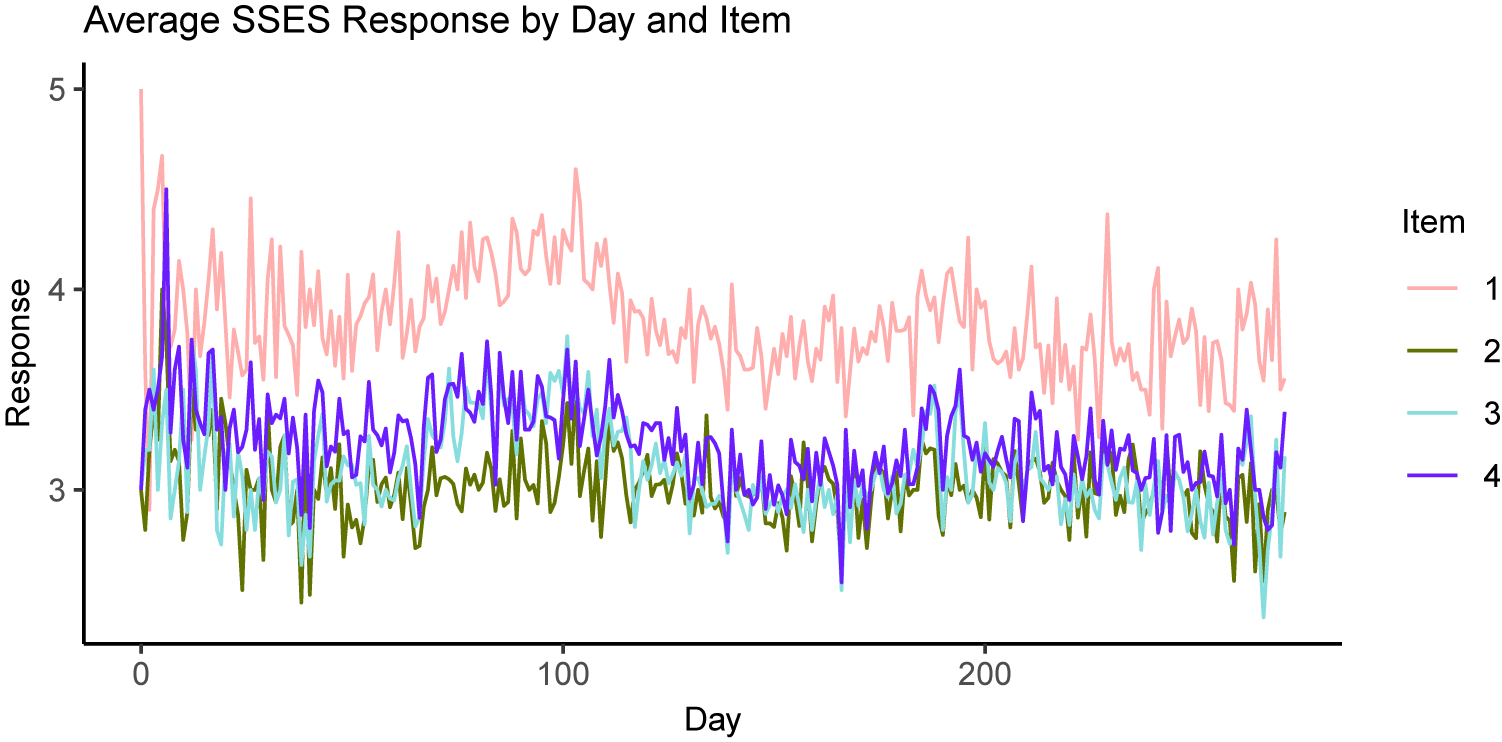
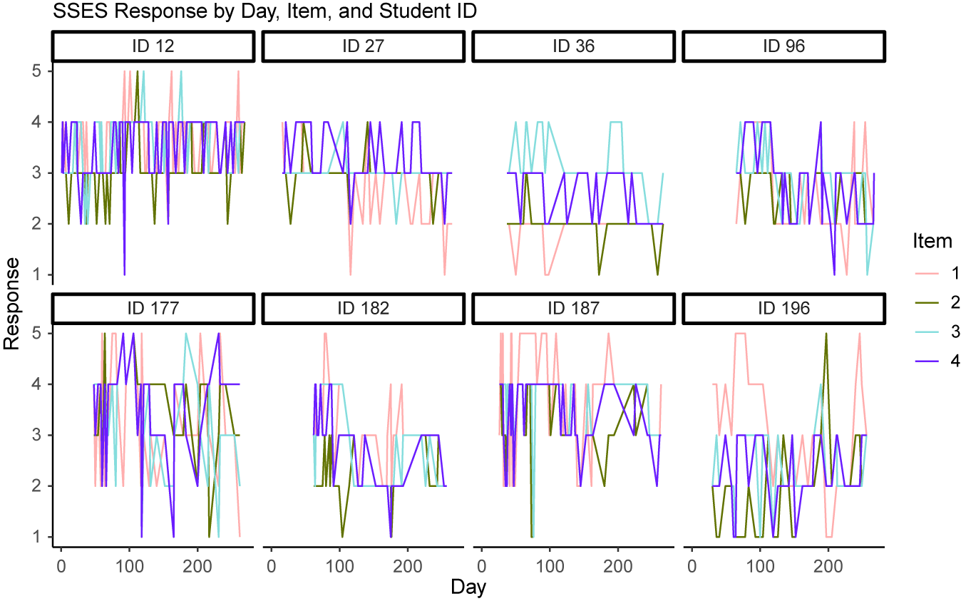
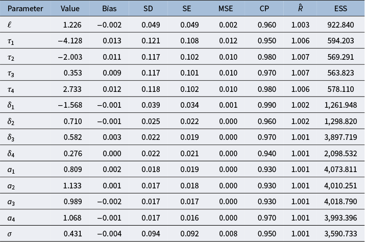

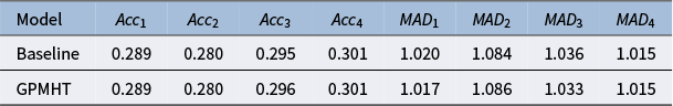

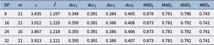

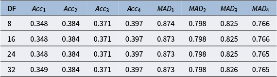
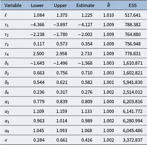

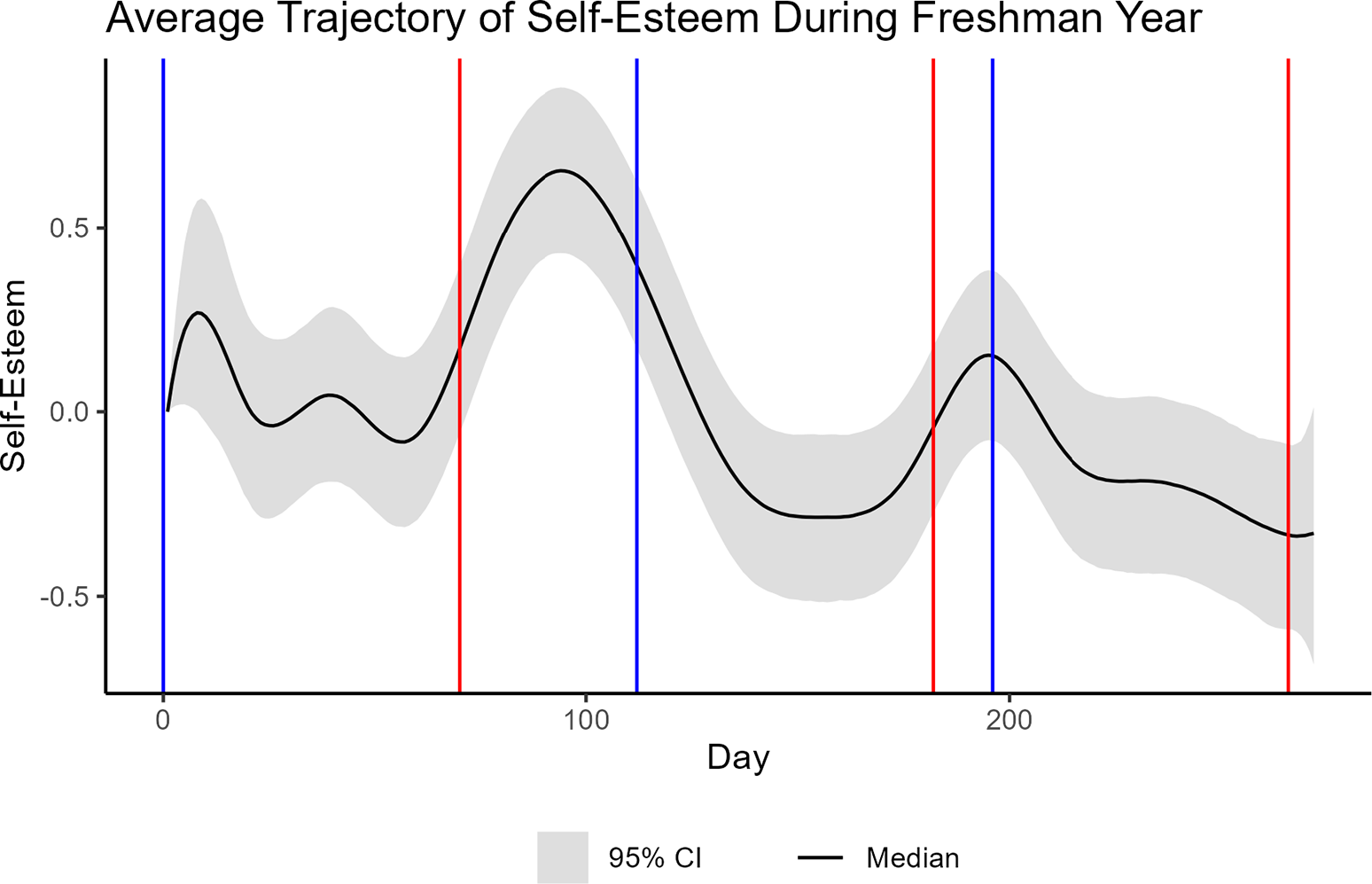
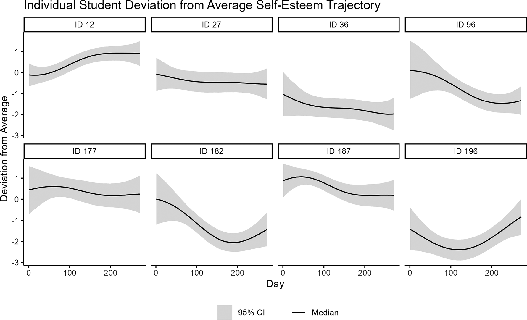
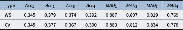
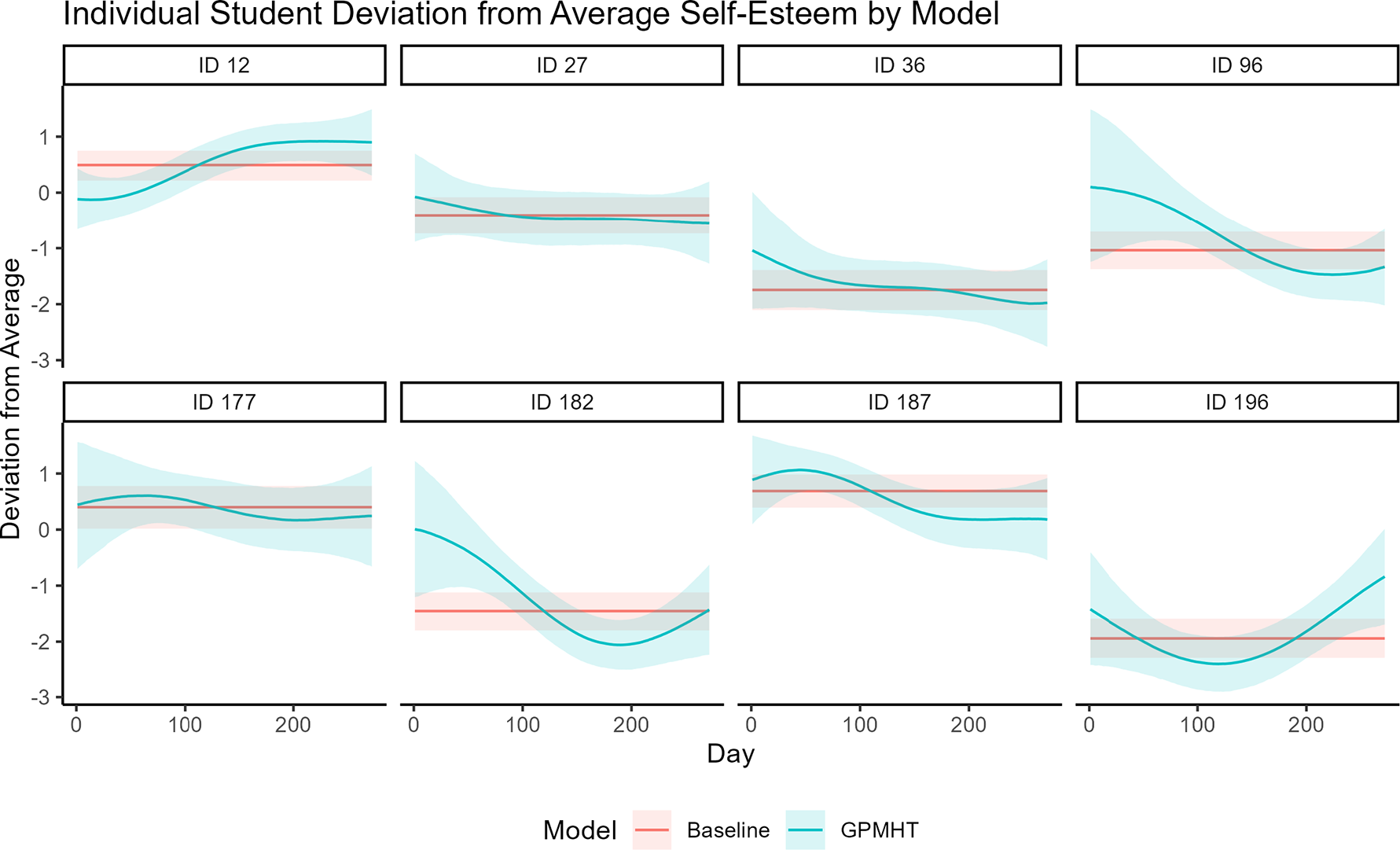
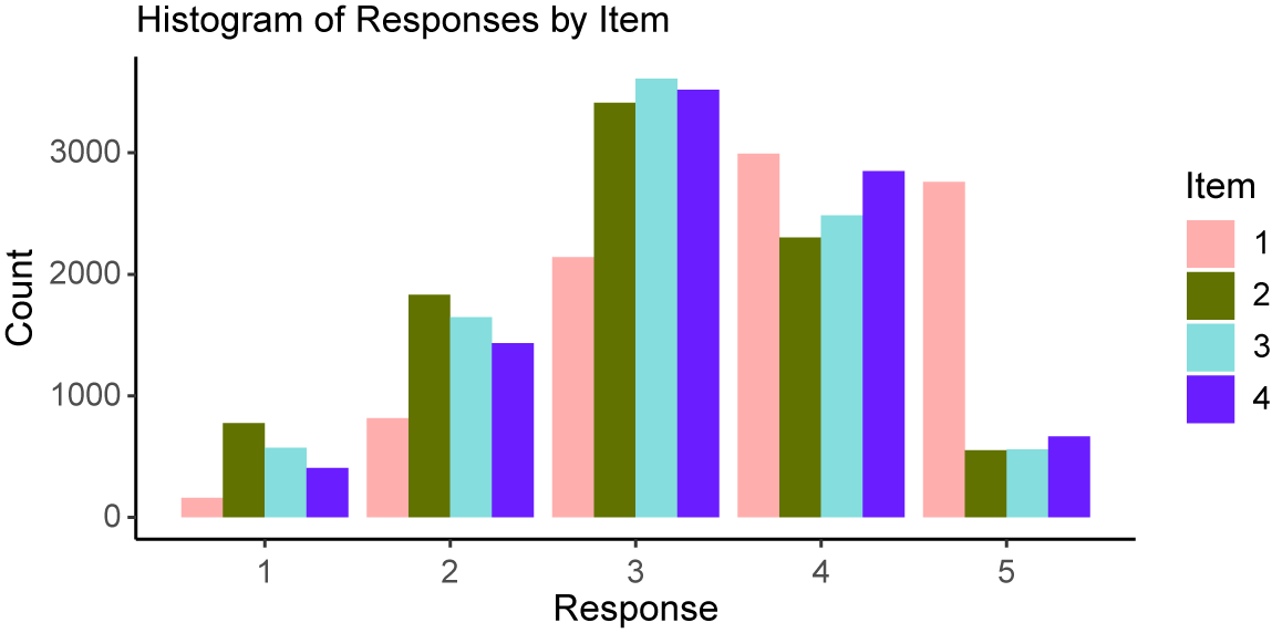
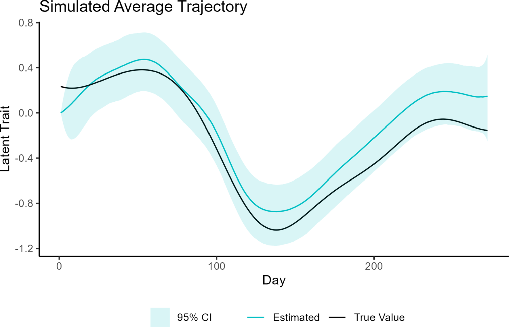


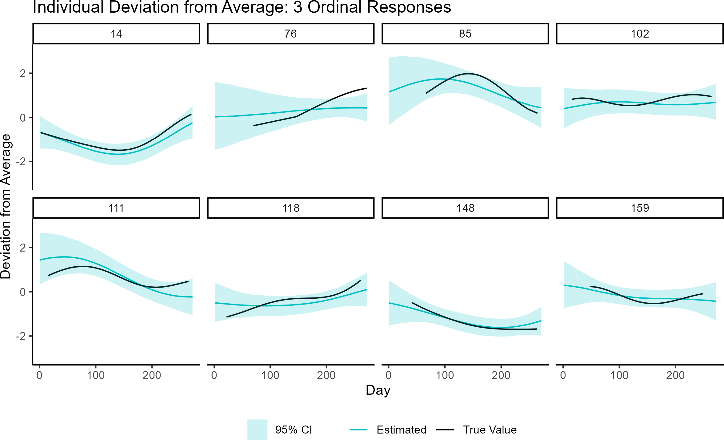


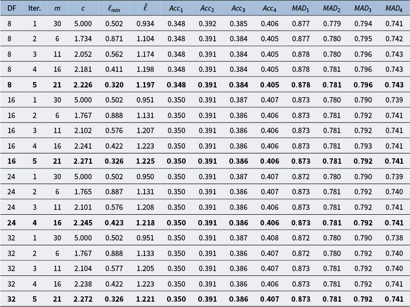

 Open access