

1 Introduction
1.1 Background
The main objective of proof-theoretic semantics is to explain the meaning of sentences in terms of proof-conditions rather than truth-conditions [Reference Schroeder-Heister, Zalta and Nodelman59]. Within the framework of Gentzen-style natural deduction, proof-theoretic semantics rests on the idea that the proof-condition of a compound sentence is explained in terms of what counts as a canonical (closed) derivation.Footnote 1 Accordingly, we know the meaning of a compound sentence when we know what counts as its canonical derivation.
A canonical derivation of a compound sentence $\mathsf {C} (A_1 , \ldots , A_n )$
, with an n-ary principal connective
$\mathsf {C} (A_1 , \ldots , A_n )$
, with an n-ary principal connective $\mathsf {C}$
, is a valid (i.e., correct) derivation whose last rule is an introduction rule of
$\mathsf {C}$
, is a valid (i.e., correct) derivation whose last rule is an introduction rule of $\mathsf {C}$
. This indicates that the introduction rules of the connective
$\mathsf {C}$
. This indicates that the introduction rules of the connective $\mathsf {C}$
play a privileged role in fixing the meaning of a compound sentence whose principal connective is
$\mathsf {C}$
play a privileged role in fixing the meaning of a compound sentence whose principal connective is $\mathsf {C}$
. Indeed, as Gentzen remarks, the introduction rules of a connective represent the ‘definitions’ of this connective, while its elimination rules are the ‘consequences’ of these definitions [Reference Szabo64, p. 80].Footnote
2
$\mathsf {C}$
. Indeed, as Gentzen remarks, the introduction rules of a connective represent the ‘definitions’ of this connective, while its elimination rules are the ‘consequences’ of these definitions [Reference Szabo64, p. 80].Footnote
2
To assign a more precise sense to Gentzen’s remark, Prawitz formulated the inversion principle, which maintains that by an application of an elimination rule, one simply ‘restores what had already been established if the major premise of the application was inferred by an application of an introduction rule’ [Reference Prawitz49, p. 33]. Consider, for instance, the introduction and elimination rules for the connective $\land $
:
$\land $
:
If $\land _I$
determines the meaning of
$\land _I$
determines the meaning of $\land $
, then by stating
$\land $
, then by stating $A \land B$
, we should not be allowed to deduce anything more than what we can already obtain from the derivations of the premises of
$A \land B$
, we should not be allowed to deduce anything more than what we can already obtain from the derivations of the premises of $\land _I$
. Therefore, Prawitz’s inversion principle can be rephrased as follows: the application of an elimination rule
$\land _I$
. Therefore, Prawitz’s inversion principle can be rephrased as follows: the application of an elimination rule $\land _E$
is dispensable when its major premise is the conclusion of the introduction rule
$\land _E$
is dispensable when its major premise is the conclusion of the introduction rule $\land _I$
, as shown by the (operation of) proof reduction below (noted with
$\land _I$
, as shown by the (operation of) proof reduction below (noted with $\rhd $
):
$\rhd $
):

The left-hand derivation is what Prawitz calls a ‘detour’ [Reference Prawitz49, p. 34] and Dummett a ‘local peak’ [Reference Dummett19, p. 248].
Several subsequent works [Reference Francez and Dyckhoff23, Reference Pfenning and Davies46, Reference Schroeder-Heister58] attempted to improve Prawitz’s analysis of Gentzen’s remark by coupling the inversion principle with the recovery principle, according to Schroeder-Heister’s terminology [Reference Schroeder-Heister58]. The recovery principle, which is often said to be the ‘converse’ of the inversion principle, consists in asking that what we can deduce by stating $A \land B$
should not be anything less than what we can already obtain from the derivations of the premises of
$A \land B$
should not be anything less than what we can already obtain from the derivations of the premises of $\land _I$
. In particular, this requires that we can recover the
$\land _I$
. In particular, this requires that we can recover the $\land _I$
rule from the assertion
$\land _I$
rule from the assertion $A \land B$
, as shown by the (operation of) proof expansion below (noted with
$A \land B$
, as shown by the (operation of) proof expansion below (noted with $\lhd $
, which is the opposite of
$\lhd $
, which is the opposite of $\rhd $
):
$\rhd $
):

The connectives whose inference rules satisfy both the inversion and the recovery principle are said to be harmonious [Reference Francez and Dyckhoff23].Footnote
3
Asking for both the inversion and the recovery principle is a way of demanding that the meaning of a connective $\mathsf {C}$
is entirely determined by its introduction rules: to fix the meaning of
$\mathsf {C}$
is entirely determined by its introduction rules: to fix the meaning of $\mathsf {C}$
, and thus of a compound sentence whose principal connective is
$\mathsf {C}$
, and thus of a compound sentence whose principal connective is $\mathsf {C}$
, all we need are the inference rules for
$\mathsf {C}$
, all we need are the inference rules for $\mathsf {C}$
; there is no need to look for any context (external to the rules of
$\mathsf {C}$
; there is no need to look for any context (external to the rules of $\mathsf {C}$
) in which to fix the reference of this connective. This is why proof-theoretic semantics is considered a non-referentialist semantics [Reference Murzi, Steinberger, Hale, Wright and Miller40], and harmony is intended as a condition for logicality, though it is considered only a necessary condition. §2 will clarify this point.
$\mathsf {C}$
) in which to fix the reference of this connective. This is why proof-theoretic semantics is considered a non-referentialist semantics [Reference Murzi, Steinberger, Hale, Wright and Miller40], and harmony is intended as a condition for logicality, though it is considered only a necessary condition. §2 will clarify this point.
While harmony has been considered so far from a logical perspective, it can also be discussed from a computational point of view. In particular, it is possible to elaborate a computational notion of harmony using the Curry–Howard correspondence. This correspondence concerns the possibility of establishing a formal link between proof (or deductive) systems in logic and functional languages in computer programming: formulas (or propositions) are interpreted as types, proofs as programs, and proof transformations (reductions or expansions) as computational steps (see, e.g., [Reference Barendregt, Abramsky, Gabbay and Maibaum5, Reference de Queiroz, de Oliveira and Gabbay53, Reference Sørensen and Urzyczyn63]). For instance, the correspondence between the implicative fragment of natural deduction and simply typed $\lambda $
-calculus, which can be seen as an abstract programming language, has been discussed in the literature.Footnote
4
In typed
$\lambda $
-calculus, which can be seen as an abstract programming language, has been discussed in the literature.Footnote
4
In typed $\lambda $
-calculus, there are typing rules which associate types with
$\lambda $
-calculus, there are typing rules which associate types with $\lambda $
-terms (i.e., programs): a
$\lambda $
-terms (i.e., programs): a $\lambda $
-term t, if it is typable, is classified into a type A by means of typing rules. We say that the term t belongs to the type A, or t is of type A, and write
$\lambda $
-term t, if it is typable, is classified into a type A by means of typing rules. We say that the term t belongs to the type A, or t is of type A, and write $t : A$
. In addition, each type is accompanied by some computation rules specifying how to execute the
$t : A$
. In addition, each type is accompanied by some computation rules specifying how to execute the $\lambda $
-terms which belong to this type. In this sense, a type can be considered as a classification of a program, as it indicates the behaviour of a program and how the program acts when it interacts with other programs.Footnote
5
Hence, according to the Curry–Howard correspondence, one can consider a formula in a natural deduction system as a classification of programs, an inference rule as a typing rule, and a reduction rule for proofs as a computation rule for
$\lambda $
-terms which belong to this type. In this sense, a type can be considered as a classification of a program, as it indicates the behaviour of a program and how the program acts when it interacts with other programs.Footnote
5
Hence, according to the Curry–Howard correspondence, one can consider a formula in a natural deduction system as a classification of programs, an inference rule as a typing rule, and a reduction rule for proofs as a computation rule for $\lambda $
-terms. In particular, the inversion principle and the recovery principle, which are the ingredients of harmony, can be considered as the two computation rules called
$\lambda $
-terms. In particular, the inversion principle and the recovery principle, which are the ingredients of harmony, can be considered as the two computation rules called $\beta $
-reduction and
$\beta $
-reduction and $\eta $
-expansion, respectively.Footnote
6
$\eta $
-expansion, respectively.Footnote
6
1.2 Aim and outline
Inspired by the Curry–Howard correspondence, in this paper we mainly focus on harmony from a computational point of view. However, our approach differs from a full-fledged interpretation of the Curry–Howard correspondence because, while the Curry–Howard correspondence states that a proposition corresponds to a type, and vice versa, our interpretation does not always require a type to correspond to a proposition.Footnote 7 This means that we emphasise the conception of type as a classification of a program rather than the proposition-as-type conception. In this respect, the computational systems we present in §3 have to be considered as typing systems which do not fully enjoy a Curry–Howard interpretation.
More specifically, we examine various computational properties of the ‘Bullet connectives’ previously introduced by Read [Reference Read54, Reference Read55]. As he showed, these connectives are harmonious but present some problematic features. When they are used with other connectives, they allow for the derivation of a contradiction, and when detour reductions are applied to this derivation, such reductions are non-terminating. For this reason, the Bullet connectives are considered paradoxical connectives. By analysing the non-terminating phenomena, Roy Dyckhoff pointed out another problem, namely, a circularity in the explanation of the meaning of the Bullet connectives in terms of proof-conditions. In §2, we analyse Read’s and Dyckhoff’s arguments relying on Prawitz’s notion of validity. We argue that, although harmonious, the Bullet connectives cannot be considered logical from the perspective of proof-theoretic semantics. The existence of harmonious connectives that are not logical suggests that harmony can be considered only a necessary condition for logicality, but not a sufficient one.
In §3, we consider harmony from a computational angle, arguing that the Bullet connectives are computationally meaningful, as they have several useful computational properties induced by their harmonious behaviour. To show this, we first reformulate the inference and the reduction rules of the Bullet connectives within a system inspired by the Curry–Howard correspondence. In particular, we consider the inference rules of this system as typing rules, and its proof-reduction rules as term-reduction rules (or computation rules). However, Read’s and Dyckhoff’s arguments against the logicality of the Bullet connectives show that the types defined in this system cannot be considered propositions. This is why our typing system ultimately deviates from enjoying a genuine Curry–Howard correspondence.
Once we have set our typing systems, we show that the behaviour of the general fixed-point operator ${\mathsf {fix}}$
, which has been discussed in the context of Martin-Löf type theory (e.g., [Reference Martin-Löf, Martin-Löf and Mints35, Reference Palmgren43]), can be simulated by means of this computational reformulation of Read’s generalised Bullet connective
${\mathsf {fix}}$
, which has been discussed in the context of Martin-Löf type theory (e.g., [Reference Martin-Löf, Martin-Löf and Mints35, Reference Palmgren43]), can be simulated by means of this computational reformulation of Read’s generalised Bullet connective $\bullet ^{A}$
[Reference Read55]. The connective
$\bullet ^{A}$
[Reference Read55]. The connective $\bullet ^A$
is also shown to be an instance of the non-normalising recursive types (which are presented, for instance, in [Reference Gunter24]). This allows us to compare
$\bullet ^A$
is also shown to be an instance of the non-normalising recursive types (which are presented, for instance, in [Reference Gunter24]). This allows us to compare $\bullet ^A$
with the recursive types in terms of type isomorphisms [Reference Bruce, Longo and Sedgewick10, Reference di Cosmo16]. In particular, while
$\bullet ^A$
with the recursive types in terms of type isomorphisms [Reference Bruce, Longo and Sedgewick10, Reference di Cosmo16]. In particular, while $\bullet ^A$
can only be proved to be isomorphic with
$\bullet ^A$
can only be proved to be isomorphic with $\bullet ^A \to A$
, we show that a recursive type
$\bullet ^A \to A$
, we show that a recursive type ${\mathsf {Ref}}$
can be defined, allowing a stronger isomorphism—namely, the one between
${\mathsf {Ref}}$
can be defined, allowing a stronger isomorphism—namely, the one between ${\mathsf {Ref}}$
and
${\mathsf {Ref}}$
and ${\mathsf {Ref}} \to {\mathsf {Ref}}$
. Next, we prove that type-free (i.e., untyped)
${\mathsf {Ref}} \to {\mathsf {Ref}}$
. Next, we prove that type-free (i.e., untyped) $\lambda $
-calculus is interpretable in simply typed
$\lambda $
-calculus is interpretable in simply typed $\lambda $
-calculus extended with yet another variant of Bullet connectives denoted by
$\lambda $
-calculus extended with yet another variant of Bullet connectives denoted by ${\bullet ^{\ast }}$
below. Finally, we discuss the computational meaning of the Bullet connectives in terms of Nakano’s modality [Reference Nakano41] in typed
${\bullet ^{\ast }}$
below. Finally, we discuss the computational meaning of the Bullet connectives in terms of Nakano’s modality [Reference Nakano41] in typed $\lambda $
-calculus: one can derive the type of Nakano’s fixed-point operator in simply typed
$\lambda $
-calculus: one can derive the type of Nakano’s fixed-point operator in simply typed $\lambda $
-calculus with the
$\lambda $
-calculus with the $\bullet ^A$
-introduction rule only.Footnote
8
We show then that one can also interpret the
$\bullet ^A$
-introduction rule only.Footnote
8
We show then that one can also interpret the $\bullet ^A$
-introduction rule in Nakano’s type system. This provides the
$\bullet ^A$
-introduction rule in Nakano’s type system. This provides the $\bullet ^A$
-introduction rule with a computational meaning in his type system.
$\bullet ^A$
-introduction rule with a computational meaning in his type system.
Our main contributions in this paper can be summarised as follows:
-
▶ We provide a precise analysis of the circularity issue regarding the definition of the Bullet connectives raised by Dyckhoff by appealing to Prawitz’s notion of validity.
-
▶ We show that the Bullet connectives are computationally meaningful as:
-
– the general fixed-point operator ${\mathsf {fix}}$
can be defined by means of the computational reformulation of Read’s generalised Bullet connective
$\bullet ^{A}$
;
${\mathsf {fix}}$
can be defined by means of the computational reformulation of Read’s generalised Bullet connective
$\bullet ^{A}$
; -
– the connective
$\bullet ^A$
is an instance of recursive types and is isomorphic only with
$\bullet ^A \to A$
, while it is possible to define a recursive type
${\mathsf {Ref}}$
such that
${\mathsf {Ref}}$
and
${\mathsf {Ref}} \to {\mathsf {Ref}}$
are isomorphic; -
– type-free
$\lambda $
-calculus is interpretable in simply typed
$\lambda $
-calculus extended with yet another variant of the Bullet connectives; -
– the type of Nakano’s fixed-point operator is derivable in simply typed
$\lambda $
-calculus with the
$\bullet ^A$
-introduction rule only, whereas the
$\bullet ^A$
-introduction rule is interpretable in Nakano’s type system.
-


2 Read’s Bullet connective
In this section, we first recall two formulations of Read’s Bullet connective, $\bullet $
, both yielding the derivation of a contradiction as well as the non-termination of detour reductions (§2.1). We then discuss Dyckhoff’s remark about the circularity of
$\bullet $
, both yielding the derivation of a contradiction as well as the non-termination of detour reductions (§2.1). We then discuss Dyckhoff’s remark about the circularity of $\bullet $
, and we make this remark more precise by appealing to Prawitz’s notion of validity (§2.2).
$\bullet $
, and we make this remark more precise by appealing to Prawitz’s notion of validity (§2.2).
2.1 Two formulations of the Bullet connective
We adopt the following notational convention concerning derivational systems (in particular, natural deduction systems): when we write some derivations where the discharge of open assumptions and the composition of derivations are at play, as in this case

we denote with the index k the fact that the application of $\to _I$
discharges n occurrences of an open assumption A (
$\to _I$
discharges n occurrences of an open assumption A ( $n \geq 0$
) annotated with k. In addition,
$n \geq 0$
) annotated with k. In addition, $\mathcal {D}_1$
denotes a derivation from an open assumption A to the conclusion (or the end formula) B, possibly containing some other open assumptions. Similarly,
$\mathcal {D}_1$
denotes a derivation from an open assumption A to the conclusion (or the end formula) B, possibly containing some other open assumptions. Similarly, $\mathcal {D}_2$
denotes a derivation of A, possibly containing some open assumptions. The right-hand derivation is then obtained by substituting n copies of
$\mathcal {D}_2$
denotes a derivation of A, possibly containing some open assumptions. The right-hand derivation is then obtained by substituting n copies of $\mathcal {D}_2$
for n occurrences of an open assumption A in
$\mathcal {D}_2$
for n occurrences of an open assumption A in $\mathcal {D}_1$
.
$\mathcal {D}_1$
.
Let us now recall two formulations of the introduction and elimination rules of $\bullet $
, which is a
$\bullet $
, which is a $0$
-ary connective, thus corresponding to an atomic formula. The first formulation is the pair
$0$
-ary connective, thus corresponding to an atomic formula. The first formulation is the pair $\bullet 1_I$
and
$\bullet 1_I$
and $\bullet 1_E$
below (see [Reference Read55, sec. 7]); if we then define
$\bullet 1_E$
below (see [Reference Read55, sec. 7]); if we then define $\neg A$
as
$\neg A$
as $A \to \bot $
, a second formulation of the rules of
$A \to \bot $
, a second formulation of the rules of $\bullet $
can be given as the pair
$\bullet $
can be given as the pair $\bullet 2_I$
and
$\bullet 2_I$
and $\bullet 2_E$
(see [Reference Read54, sec. 2.8])Footnote
9
:
$\bullet 2_E$
(see [Reference Read54, sec. 2.8])Footnote
9
:

One can easily see that these two formulations are equivalent, namely, each pair of introduction and elimination rules is derivable from the other pair by means of the inference rules of $\to $
. The second formulation, however, gives a very intuitive idea of the behaviour of
$\to $
. The second formulation, however, gives a very intuitive idea of the behaviour of $\bullet $
: it corresponds to a formula which is logically equivalent to its negation. This is why Read interprets
$\bullet $
: it corresponds to a formula which is logically equivalent to its negation. This is why Read interprets $\bullet $
as a ‘proof-conditional Liar sentence’ [Reference Read54, p. 142] or, alternatively, as corresponding to Russell’s paradox formula
$\bullet $
as a ‘proof-conditional Liar sentence’ [Reference Read54, p. 142] or, alternatively, as corresponding to Russell’s paradox formula $r \in r,$
where
$r \in r,$
where $r = \{ x \mid x \not \in x \}$
([Reference Read55, p. 574]; cf. also Tranchini [Reference Tranchini67, sec. 2] about this second interpretation). For this reason, one can take
$r = \{ x \mid x \not \in x \}$
([Reference Read55, p. 574]; cf. also Tranchini [Reference Tranchini67, sec. 2] about this second interpretation). For this reason, one can take $\bullet $
to be ‘a paradoxical connective’ (we will better clarify this point later).
$\bullet $
to be ‘a paradoxical connective’ (we will better clarify this point later).
Each of these two formulations satisfies the inversion principle, as already shown by Read in [Reference Read54, Reference Read55] (in his terms, each satisfies harmony); also, each of them satisfies the recovery principle:

The fact that $\bullet $
satisfies both the inversion and the recovery principles makes it comparable to the standard connectives (like conjunction, disjunction, and implication), which also satisfy these two principles. Up to this point,
$\bullet $
satisfies both the inversion and the recovery principles makes it comparable to the standard connectives (like conjunction, disjunction, and implication), which also satisfy these two principles. Up to this point, $\bullet $
meets all the relevant conditions to be a ‘good’ candidate as a logical connective.Footnote
10
$\bullet $
meets all the relevant conditions to be a ‘good’ candidate as a logical connective.Footnote
10
However, Read showed that each of the two formulations yields a contradiction:

Read also showed in [Reference Read55] that the reduction of the first contradictory derivation is non-terminating, and it is not hard to see the non-termination of the reduction of the second as well. The absence of contradiction has been traditionally considered (since Aristotle) one of the characteristic features of any logical and meaningful discourse. The fact that $\bullet $
brings about a contradiction seems then to make a point against its logicality and meaningfulness, although it satisfies the harmony condition.Footnote
11
$\bullet $
brings about a contradiction seems then to make a point against its logicality and meaningfulness, although it satisfies the harmony condition.Footnote
11
2.2 The circularity of the Bullet connective
By analysing the problems of contradiction and non-termination we just exposed, Dyckhoff identifies another issue concerning $\bullet $
from the point of view of proof-theoretic semantics [Reference Dyckhoff, Piecha and Schroeder-Heister20, p. 82]. He considers the first formulation of the inference rules for
$\bullet $
from the point of view of proof-theoretic semantics [Reference Dyckhoff, Piecha and Schroeder-Heister20, p. 82]. He considers the first formulation of the inference rules for $\bullet $
, and following the meaning-explanation of propositions as given by [Reference Dummett19, Reference Martin-Löf34, Reference Martin-Löf36], he claims that ‘we understand a proposition when we understand what it means to have a canonical proof of it, i.e. what forms a canonical proof can take’ [Reference Dyckhoff, Piecha and Schroeder-Heister20, p. 82]. By a ‘canonical proof’, Dyckhoff means a derivation whose last rule is an introduction rule. According to him, the first formulation of the introduction rule for
$\bullet $
, and following the meaning-explanation of propositions as given by [Reference Dummett19, Reference Martin-Löf34, Reference Martin-Löf36], he claims that ‘we understand a proposition when we understand what it means to have a canonical proof of it, i.e. what forms a canonical proof can take’ [Reference Dyckhoff, Piecha and Schroeder-Heister20, p. 82]. By a ‘canonical proof’, Dyckhoff means a derivation whose last rule is an introduction rule. According to him, the first formulation of the introduction rule for $\bullet $
attempts to explain what a canonical proof for
$\bullet $
attempts to explain what a canonical proof for $\bullet $
is: this rule says that a canonical proof for
$\bullet $
is: this rule says that a canonical proof for $\bullet $
is a proof obtained by applying
$\bullet $
is a proof obtained by applying $\bullet 1_I$
-rule to a derivation from
$\bullet 1_I$
-rule to a derivation from $\bullet $
to
$\bullet $
to $\bot $
. Dyckhoff treats the subderivation
$\bot $
. Dyckhoff treats the subderivation $\mathcal {D}$
as a method for transforming arbitrary proofs of
$\mathcal {D}$
as a method for transforming arbitrary proofs of $\bullet $
into proofs of
$\bullet $
into proofs of $\bot $
, and he finds a circularity in the alleged explanation. That is, the above explanation of canonical proofs for
$\bot $
, and he finds a circularity in the alleged explanation. That is, the above explanation of canonical proofs for $\bullet $
presupposes the notion of proof of
$\bullet $
presupposes the notion of proof of $\bullet $
, in particular the notion of canonical proof for
$\bullet $
, in particular the notion of canonical proof for $\bullet $
.
$\bullet $
.
What stands behind Dyckhoff’s remark is in fact a well-founded and hierarchical view of proofs. A typical instance of such a view is given by the Brouwer–Heyting–Kolmogorov interpretation (the BHK-interpretation, for short; see [Reference Troelstra and van Dalen70, pp. 9–10]). The BHK-interpretation is an informal explanation of the meaning of intuitionistic logic. In particular, proofs in this interpretation stand for any kind of objects provided by (idealised) mathematicians in order to give evidence to their claims. The domain of such proofs is constructed bottom-up, and this construction proceeds along a certain hierarchical structure. As explained by van Atten, this view essentially follows Brouwer’s intuitionism:
[ $\ldots $
] in our mathematical acts we first construct certain basic objects, [
$\ldots $
] in our mathematical acts we first construct certain basic objects, [ $\ldots $
] and then to those apply the same mathematical acts to construct further objects. This activity thus has an iterative structure, and induces a linear order on the constructions that the Creating Subject has effected. [
$\ldots $
] and then to those apply the same mathematical acts to construct further objects. This activity thus has an iterative structure, and induces a linear order on the constructions that the Creating Subject has effected. [ $\ldots $
] As the linear ordering of the Creating Subject’s constructions is not only the order in which it becomes aware of the objects, but indeed the order in which they come into being, this order is a mathematical fact. [Reference van Atten3, p. 1598]
$\ldots $
] As the linear ordering of the Creating Subject’s constructions is not only the order in which it becomes aware of the objects, but indeed the order in which they come into being, this order is a mathematical fact. [Reference van Atten3, p. 1598]
If we read Dyckhoff’s remark about the circularity of $\bullet $
in the light of this passage, we can interpret it as suggesting that a well-founded and hierarchical domain of proofs cannot be constructed—even by some idealised mathematician, like the Creative Subject—in the case of
$\bullet $
in the light of this passage, we can interpret it as suggesting that a well-founded and hierarchical domain of proofs cannot be constructed—even by some idealised mathematician, like the Creative Subject—in the case of $\bullet $
.
$\bullet $
.
More precisely, we spell out Dyckhoff’s idea by showing that if we try to define in a bottom-up way a domain of proofs by using the $\bullet $
-rules, we eventually end up with a circular definition. Since the BHK-interpretation is an informal one, we replace it by appealing to a formal notion, that of Prawitz’s validity. This notion indeed includes a well-founded and hierarchical perspective of proofs, as the one considered above, although proofs are taken here to be closed derivations in the natural deduction format (see the definition below). The formulation of validity which we adopt here is a simplified version of the one given in [Reference Prawitz and Fenstad50, Reference Schroeder-Heister56].Footnote
12
$\bullet $
-rules, we eventually end up with a circular definition. Since the BHK-interpretation is an informal one, we replace it by appealing to a formal notion, that of Prawitz’s validity. This notion indeed includes a well-founded and hierarchical perspective of proofs, as the one considered above, although proofs are taken here to be closed derivations in the natural deduction format (see the definition below). The formulation of validity which we adopt here is a simplified version of the one given in [Reference Prawitz and Fenstad50, Reference Schroeder-Heister56].Footnote
12
A derivation $\mathcal {D}$
is closed if it has no open assumption; otherwise,
$\mathcal {D}$
is closed if it has no open assumption; otherwise, $\mathcal {D}$
is said to be open. An atomic system is a pair composed of an arbitrary set
$\mathcal {D}$
is said to be open. An atomic system is a pair composed of an arbitrary set $\mathcal {P}$
of atomic formulas including
$\mathcal {P}$
of atomic formulas including $\bot $
and an arbitrary set
$\bot $
and an arbitrary set $\mathcal {R}$
of inference rules of the form
$\mathcal {R}$
of inference rules of the form
such that
-
(i)
$n \geq 0$
, -
(ii)
$\{ A , A_1 ,\ldots , A_n \} \subseteq \mathcal {P}$
, and -
(iii) no closed derivation of
$\bot $
can be obtained by using the inference rules of
$\mathcal {R}$
.


When $n = 0$
holds, the inference rule is an axiom which states that A holds. In the rest of this subsection, we consider formulas to be given relative to an atomic system
$n = 0$
holds, the inference rule is an axiom which states that A holds. In the rest of this subsection, we consider formulas to be given relative to an atomic system $\mathcal {S}$
: formulas are constructed by a given set of logical connectives from atomic formulas in
$\mathcal {S}$
: formulas are constructed by a given set of logical connectives from atomic formulas in $\mathcal {S}$
. For an atomic system
$\mathcal {S}$
. For an atomic system $\mathcal {S}$
, a derivation in
$\mathcal {S}$
, a derivation in $\mathcal {S}$
is a derivation which contains inference rules in
$\mathcal {S}$
is a derivation which contains inference rules in $\mathcal {S}$
only. Closed derivations in an atomic system
$\mathcal {S}$
only. Closed derivations in an atomic system $\mathcal {S}$
are the basic proofs on which a domain of proofs is constructed in a bottom-up way. For a finite set
$\mathcal {S}$
are the basic proofs on which a domain of proofs is constructed in a bottom-up way. For a finite set $\{ A_1 , \ldots , A_n \}$
of formulas, we define its complexity as the number of all occurrences of connectives in this set. The complexity of a formula A is defined as the complexity of
$\{ A_1 , \ldots , A_n \}$
of formulas, we define its complexity as the number of all occurrences of connectives in this set. The complexity of a formula A is defined as the complexity of $\{ A \}$
.
$\{ A \}$
.
In order to introduce Prawitz’s notion of validity for $\bullet $
, we first formulate the notion of validity for derivations which contain only the rules of a given atomic system
$\bullet $
, we first formulate the notion of validity for derivations which contain only the rules of a given atomic system $\mathcal {S}$
and the rules for
$\mathcal {S}$
and the rules for $\to $
.
$\to $
.
Definition 2.1 (Validity of derivations with atomic systems)
Let $\mathcal {S}$
be an atomic system. The set of
$\mathcal {S}$
be an atomic system. The set of $\mathcal {S}$
-valid derivations is defined by induction on the sum of the complexities of the open assumptions
$\mathcal {S}$
-valid derivations is defined by induction on the sum of the complexities of the open assumptions $\{ A_1 , \ldots , A_n \}$
and the end formula B:
$\{ A_1 , \ldots , A_n \}$
and the end formula B:
-
1. A closed derivation of an atomic formula is
$\mathcal {S}$
-valid if it reduces to a derivation in
$\mathcal {S}$
. -
2. A closed derivation of
$A \to B$
is
$\mathcal {S}$
-valid if it reduces to a derivation of the form and for any closed
$\mathcal {S}$
-valid derivation , the derivation is
$\mathcal {S}$
-valid.
-
3. An open derivation of the form
is
$\mathcal {S}$
-valid if for any closed
$\mathcal {S}$
-valid derivation with
$1 \leq i \leq n$
, the derivation is
$\mathcal {S}$
-valid.


Using the notion of $\mathcal {S}$
-validity, we can now explain better the circularity of the
$\mathcal {S}$
-validity, we can now explain better the circularity of the $\bullet $
-rules. The inductive definition of validity breaks once we add the clause for defining the validity of a closed derivation of
$\bullet $
-rules. The inductive definition of validity breaks once we add the clause for defining the validity of a closed derivation of $\bullet $
: by adding this clause, we get a circular definition. Consider the first formulation of the
$\bullet $
: by adding this clause, we get a circular definition. Consider the first formulation of the $\bullet $
-rules, and suppose that we try to define the
$\bullet $
-rules, and suppose that we try to define the $\mathcal {S}$
-validity of a derivation by induction on the sum of the complexities of its open assumptions and the end formula. The similarity between
$\mathcal {S}$
-validity of a derivation by induction on the sum of the complexities of its open assumptions and the end formula. The similarity between $\bullet 1_I$
and
$\bullet 1_I$
and $\to _I$
suggests considering the following clause:
$\to _I$
suggests considering the following clause:
-
(B) A closed derivation of
$\bullet $
is
$\mathcal {S}$
-valid if it reduces to a derivation of the form and for any closed
$\mathcal {S}$
-valid derivation , the derivation is
$\mathcal {S}$
-valid.


Here the $\mathcal {S}$
-validity of a closed derivation of
$\mathcal {S}$
-validity of a closed derivation of $\bullet $
depends on the validity of arbitrary closed
$\bullet $
depends on the validity of arbitrary closed $\mathcal {S}$
-valid derivations having the same conclusion, i.e.,
$\mathcal {S}$
-valid derivations having the same conclusion, i.e., ![]() . This implies that the inductive clause (B) does not decrease the joint complexity of the open assumptions and the end formula, since the derivations considered are all closed, valid, and have the same complexity as the conclusion. Therefore, the inductive definition breaks down, and the clause leads to a circularity, as point out by Dyckhoff. The second formulation of the
. This implies that the inductive clause (B) does not decrease the joint complexity of the open assumptions and the end formula, since the derivations considered are all closed, valid, and have the same complexity as the conclusion. Therefore, the inductive definition breaks down, and the clause leads to a circularity, as point out by Dyckhoff. The second formulation of the $\bullet $
-rules breaks the inductive definition as well.
$\bullet $
-rules breaks the inductive definition as well.
To sum up, the introduction and elimination rules for $\bullet $
satisfy both the inversion principle and the recovery principle (whenever we adopt the first formulation or the second formulation). However, these rules yield a contradiction, and derivations of such a contradiction do not admit a normal form. Moreover, as Dyckhoff remarks, when these rules are analysed from the point of proof-theoretic semantics, the
$\bullet $
satisfy both the inversion principle and the recovery principle (whenever we adopt the first formulation or the second formulation). However, these rules yield a contradiction, and derivations of such a contradiction do not admit a normal form. Moreover, as Dyckhoff remarks, when these rules are analysed from the point of proof-theoretic semantics, the $\bullet $
-rules present a form of circularity, which can be made explicit by appealing to Prawtiz’s notion of validity, as we have just shown.
$\bullet $
-rules present a form of circularity, which can be made explicit by appealing to Prawtiz’s notion of validity, as we have just shown.
Considering $\bullet $
through Prawitz’s validity, we can specify that deriving a contradiction is highly undesirable and makes it problematic to consider
$\bullet $
through Prawitz’s validity, we can specify that deriving a contradiction is highly undesirable and makes it problematic to consider $\bullet $
to be a (
$\bullet $
to be a ( $0$
-ary) logical connective. Although
$0$
-ary) logical connective. Although $\bullet $
is harmonious, and thus satisfies a necessary condition to be a logical connective, the derivation of a contradiction makes it possible to produce non-valid derivations in the sense of Prawitz. The derivations of
$\bullet $
is harmonious, and thus satisfies a necessary condition to be a logical connective, the derivation of a contradiction makes it possible to produce non-valid derivations in the sense of Prawitz. The derivations of $\bot $
that we have seen on p. 7 are closed and non-canonical; hence, by applying the rule of ex falso quodlibet, it is possible to obtain closed and non-canonical derivations of any formula. In particular, we can obtain a closed derivation for any atomic formula. Among these formulas, there is also
$\bot $
that we have seen on p. 7 are closed and non-canonical; hence, by applying the rule of ex falso quodlibet, it is possible to obtain closed and non-canonical derivations of any formula. In particular, we can obtain a closed derivation for any atomic formula. Among these formulas, there is also $\bullet $
(since a
$\bullet $
(since a $0$
-ary connective corresponds to an atomic proposition), and such a derivation cannot be reduced to a derivation in any atomic system. We are considering logical validity and no atomic rules are given. Moreover, the rules of
$0$
-ary connective corresponds to an atomic proposition), and such a derivation cannot be reduced to a derivation in any atomic system. We are considering logical validity and no atomic rules are given. Moreover, the rules of $\bullet $
(in both formulations) cannot themselves belong to any atomic system: in the first formulation, the
$\bullet $
(in both formulations) cannot themselves belong to any atomic system: in the first formulation, the $\bullet $
-introduction rule can discharge finitely many assumptions of the form
$\bullet $
-introduction rule can discharge finitely many assumptions of the form $\bullet $
, while in the second formulation the connective
$\bullet $
, while in the second formulation the connective $\neg $
occurs in the
$\neg $
occurs in the $\bullet $
-rules, so that in both cases we are not respecting the format of atomic rules given at p. 8.Footnote
13
Thus, this situation makes the first clause of Prawitz’s validity false. In fact, the situation would be problematic also if we consider arbitrary formulas instead of atomic ones. The application of the ex falso quodlibet to the two closed derivations of
$\bullet $
-rules, so that in both cases we are not respecting the format of atomic rules given at p. 8.Footnote
13
Thus, this situation makes the first clause of Prawitz’s validity false. In fact, the situation would be problematic also if we consider arbitrary formulas instead of atomic ones. The application of the ex falso quodlibet to the two closed derivations of $\bot $
considered at p. 7 makes it possible to obtain a closed derivation of
$\bot $
considered at p. 7 makes it possible to obtain a closed derivation of $A \to B$
, for any A and B. This is a derivation that cannot be reduced to a derivation ending with the
$A \to B$
, for any A and B. This is a derivation that cannot be reduced to a derivation ending with the $\to $
-introduction rule, so that in this case it is the second clause of Prawitz’s validity definition which would become false.
$\to $
-introduction rule, so that in this case it is the second clause of Prawitz’s validity definition which would become false.
It could be objected that by dropping the ex falso quodlibet rule, the $\bullet $
-rules do not yield non-valid derivations. However, the circularity of the validity clauses for
$\bullet $
-rules do not yield non-valid derivations. However, the circularity of the validity clauses for $\bullet $
would still be problematic, as it prevents an inductive construction of the domain of proofs. The issue is whether such a conception of the domain of proofs is essential. Considering that this conception is motivated by an intuitionistic point of view, we might want to abandon it. However, if we do so, we will not only abandon one of the sources of inspiration for proof-theoretic semantics, but also one of the characteristic features shaping it. The adoption of proof-theoretic semantics is usually linked with intuitionistic logic.Footnote
14
Hence, to avoid the hierarchical and well-founded view of proofs that we mentioned, one should be able to show that proof-theoretic semantics can be defined without necessarily having to adopt an intuitionistic conception. In other words, one should show that it is possible to have a proof-theoretic semantics that does not validate intuitionistic logic. This is not the approach we want to pursue. Note that, originally, the very idea of proof-theoretic semantics rests on the BHK-interpretation (cf. [Reference Schroeder-Heister, Zalta and Nodelman59]). We consider that such a hierarchical and well-founded notion of proofs is perfectly legitimate, and that
$\bullet $
would still be problematic, as it prevents an inductive construction of the domain of proofs. The issue is whether such a conception of the domain of proofs is essential. Considering that this conception is motivated by an intuitionistic point of view, we might want to abandon it. However, if we do so, we will not only abandon one of the sources of inspiration for proof-theoretic semantics, but also one of the characteristic features shaping it. The adoption of proof-theoretic semantics is usually linked with intuitionistic logic.Footnote
14
Hence, to avoid the hierarchical and well-founded view of proofs that we mentioned, one should be able to show that proof-theoretic semantics can be defined without necessarily having to adopt an intuitionistic conception. In other words, one should show that it is possible to have a proof-theoretic semantics that does not validate intuitionistic logic. This is not the approach we want to pursue. Note that, originally, the very idea of proof-theoretic semantics rests on the BHK-interpretation (cf. [Reference Schroeder-Heister, Zalta and Nodelman59]). We consider that such a hierarchical and well-founded notion of proofs is perfectly legitimate, and that $\bullet $
is not enough to question it.
$\bullet $
is not enough to question it.
The lesson we learn from the proof-theoretic analysis of $\bullet $
is actually another one, namely, that harmony, being only a necessary but not sufficient condition for logicality, is too weak as a requirement. Moreover, it is not even a sufficient condition for meaningfulness. It is only by satisfying Prawitz’s validity that we can say that a certain connective is really meaningful from a proof-theoretic semantics point of view. More precisely, if the rules of a certain connective allow one to define a notion of proof that satisfies validity, we can then say that this connective is meaningful. In particular, this connective allows one to define propositions, that is, meaningful linguistic entities that are assertible, and for which we can give evidence.Footnote
15
The fact that the
$\bullet $
is actually another one, namely, that harmony, being only a necessary but not sufficient condition for logicality, is too weak as a requirement. Moreover, it is not even a sufficient condition for meaningfulness. It is only by satisfying Prawitz’s validity that we can say that a certain connective is really meaningful from a proof-theoretic semantics point of view. More precisely, if the rules of a certain connective allow one to define a notion of proof that satisfies validity, we can then say that this connective is meaningful. In particular, this connective allows one to define propositions, that is, meaningful linguistic entities that are assertible, and for which we can give evidence.Footnote
15
The fact that the $\bullet $
-rules do not allow one to define a notion of proof satisfying validity means that
$\bullet $
-rules do not allow one to define a notion of proof satisfying validity means that $\bullet $
does not allow one to form propositions.
$\bullet $
does not allow one to form propositions.
The notion of validity is defined inductively; one of the induction parameters is the complexity of the conclusion of a proof. Now, according to what we just said, the conclusion of a proof is not simply a formula, but a proposition. This implies that the notion of proposition must be also inductively defined, in the sense that it must be well-founded. This is consistent with the notion of proof discussed above: proofs involve propositions, and both proofs and propositions are organised in a hierarchical and well-founded way.
We will revisit the notion of proposition in §5, comparing it with the notion of type, which we will discuss in the next section.
3 The computational meaning of the Bullet connective
Read’s Bullet connective $\bullet $
is problematic from the logical point of view. In this section, we argue that this connective is nevertheless computationally meaningful, as some variants of it have several computational properties. We start by reformulating the rules for
$\bullet $
is problematic from the logical point of view. In this section, we argue that this connective is nevertheless computationally meaningful, as some variants of it have several computational properties. We start by reformulating the rules for $\bullet $
, as well as its generalisation given in [Reference Read55], within a framework inspired by the Curry–Howard correspondence (§3.1). Next, we show that the behaviour of the fixed-point operator
$\bullet $
, as well as its generalisation given in [Reference Read55], within a framework inspired by the Curry–Howard correspondence (§3.1). Next, we show that the behaviour of the fixed-point operator ${\mathsf {fix}}$
, which has been discussed in the context of Martin-Löf type theory, can be simulated with this generalisation of the Bullet connective. Moreover, we note that the generalised Bullet connective is an instance of non-normalising recursive types (§3.2). We prove then that type-free
${\mathsf {fix}}$
, which has been discussed in the context of Martin-Löf type theory, can be simulated with this generalisation of the Bullet connective. Moreover, we note that the generalised Bullet connective is an instance of non-normalising recursive types (§3.2). We prove then that type-free $\lambda $
-calculus is interpretable in simply typed
$\lambda $
-calculus is interpretable in simply typed $\lambda $
-calculus with yet another variant
$\lambda $
-calculus with yet another variant ${\bullet ^{\ast }}$
of the Bullet connective, exploiting the type isomorphism between
${\bullet ^{\ast }}$
of the Bullet connective, exploiting the type isomorphism between ${\bullet ^{\ast }}$
and
${\bullet ^{\ast }}$
and ${\bullet ^{\ast }} \to {\bullet ^{\ast }}$
(§3.3). Finally, we discuss the computational meaning of Bullet connectives in terms of Nakano’s modality [Reference Nakano41] in typed
${\bullet ^{\ast }} \to {\bullet ^{\ast }}$
(§3.3). Finally, we discuss the computational meaning of Bullet connectives in terms of Nakano’s modality [Reference Nakano41] in typed $\lambda $
-calculus (§3.4). One can derive the type of Nakano’s fixed-point operator in simply typed
$\lambda $
-calculus (§3.4). One can derive the type of Nakano’s fixed-point operator in simply typed $\lambda $
-calculus with the
$\lambda $
-calculus with the $\bullet ^A$
-introduction rule only, and we show that one can also interpret the
$\bullet ^A$
-introduction rule only, and we show that one can also interpret the $\bullet ^A$
-introduction rule in Nakano’s type system.
$\bullet ^A$
-introduction rule in Nakano’s type system.
Types and terms of $\lambda_{1}^{\to\bullet}$
.
$\lambda_{1}^{\to\bullet}$
.

3.1 The Bullet connective in the light of a computational framework
We extend simply typed $\lambda $
-calculus
$\lambda $
-calculus $\lambda ^{\to }$
(see, e.g., [Reference Sørensen and Urzyczyn63]) by adding the Bullet connective to this calculus. Given infinitely many atomic types
$\lambda ^{\to }$
(see, e.g., [Reference Sørensen and Urzyczyn63]) by adding the Bullet connective to this calculus. Given infinitely many atomic types $P_0 , P_1 , \ldots $
and variables
$P_0 , P_1 , \ldots $
and variables $x_1 , x_2 , \ldots $
, types and (untyped) terms of the extended calculus are defined as in Figure 1. We denote this calculus by
$x_1 , x_2 , \ldots $
, types and (untyped) terms of the extended calculus are defined as in Figure 1. We denote this calculus by $\lambda ^{\to \bullet}_1$
, since the constructor
$\lambda ^{\to \bullet}_1$
, since the constructor $\hat {x}. t$
and the destructor
$\hat {x}. t$
and the destructor ${@} (t , s)$
correspond to the first version of the
${@} (t , s)$
correspond to the first version of the $\bullet $
-introduction and
$\bullet $
-introduction and $\bullet $
-elimination rules, respectively.Footnote
16
In what follows, we abbreviate
$\bullet $
-elimination rules, respectively.Footnote
16
In what follows, we abbreviate $\mathsf {app}(t , s)$
as
$\mathsf {app}(t , s)$
as $t \: s$
, and write
$t \: s$
, and write ${@} (t , s)$
using the infix notation
${@} (t , s)$
using the infix notation $t {@} s$
. Note that, in the term
$t {@} s$
. Note that, in the term $\hat {x}. t$
, the variable x is bound as in the
$\hat {x}. t$
, the variable x is bound as in the $\lambda $
-abstraction term
$\lambda $
-abstraction term $\lambda x. t$
. The expression
$\lambda x. t$
. The expression $t[s / x]$
denotes the term obtained by substituting the term s for every free occurrence of the variable x in the term t. We often abbreviate
$t[s / x]$
denotes the term obtained by substituting the term s for every free occurrence of the variable x in the term t. We often abbreviate $t[s / x]$
as
$t[s / x]$
as $t[s]$
when it is obvious which variable is replaced. These notations can be extended to simultaneous substitution
$t[s]$
when it is obvious which variable is replaced. These notations can be extended to simultaneous substitution $t[s_1 / x_1 , \ldots , s_n / x_n]$
straightforwardly (which can thus be abbreviated as
$t[s_1 / x_1 , \ldots , s_n / x_n]$
straightforwardly (which can thus be abbreviated as $t[s_1 , \ldots , s_n]$
).
$t[s_1 , \ldots , s_n]$
).
A pair $(x , A)$
composed of a variable and a type is called a declaration, and it is usually written as
$(x , A)$
composed of a variable and a type is called a declaration, and it is usually written as $x : A$
. If the variables present in a set of declarations are pairwise distinct, we call this set a context, and a context is denoted by a capital Greek letter, such as
$x : A$
. If the variables present in a set of declarations are pairwise distinct, we call this set a context, and a context is denoted by a capital Greek letter, such as $\Gamma $
and
$\Gamma $
and $\Delta $
. Usual notations for contexts are adopted: for instance, a singleton
$\Delta $
. Usual notations for contexts are adopted: for instance, a singleton $\{ x : A \}$
is abbreviated as
$\{ x : A \}$
is abbreviated as $x : A$
, and we denote the union of two contexts
$x : A$
, and we denote the union of two contexts $\Gamma $
and
$\Gamma $
and $\Delta $
by
$\Delta $
by $\Gamma , \Delta $
.
$\Gamma , \Delta $
. $\lambda^{\to \bullet}_1$
-typing rules.
$\lambda^{\to \bullet}_1$
-typing rules.
 $\lambda^{\to \bullet}_2$
-typing rules.
$\lambda^{\to \bullet}_2$
-typing rules.
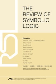
A typing judgement is an expression of the form $\Gamma \vdash t : A$
, meaning that the term t is of type A with respect to the context
$\Gamma \vdash t : A$
, meaning that the term t is of type A with respect to the context $\Gamma $
.Footnote
17
The typing rules of
$\Gamma $
.Footnote
17
The typing rules of $\lambda ^{\to \bullet}_1$
operate on this kind of judgement and are formulated in a natural deduction system, presented in a sequent-style format,Footnote
18
as in Figure 2. This allows for an alternative reading of the role of the terms, namely, that of keeping track of the natural deduction rules applied to form it, so that a judgement of the
$\lambda ^{\to \bullet}_1$
operate on this kind of judgement and are formulated in a natural deduction system, presented in a sequent-style format,Footnote
18
as in Figure 2. This allows for an alternative reading of the role of the terms, namely, that of keeping track of the natural deduction rules applied to form it, so that a judgement of the $\Gamma \vdash t : A$
can also be read as expressing the fact that t is the code of a derivation of A from the premises
$\Gamma \vdash t : A$
can also be read as expressing the fact that t is the code of a derivation of A from the premises $\Gamma $
. If we adopt the usual natural deduction format (instead of the sequent-style format), as well as the same notational conventions adopted in §2.1, the typing rules for
$\Gamma $
. If we adopt the usual natural deduction format (instead of the sequent-style format), as well as the same notational conventions adopted in §2.1, the typing rules for $\bullet $
can be presented in the following way, where the introduction and elimination rules for
$\bullet $
can be presented in the following way, where the introduction and elimination rules for $\bullet $
are decorated with appropriate terms:
$\bullet $
are decorated with appropriate terms:

We can also present the second version of the $\bullet $
-rules as typing rules. The syntax of the system
$\bullet $
-rules as typing rules. The syntax of the system $\lambda ^{\to \bullet}_2$
, which is an extension of
$\lambda ^{\to \bullet}_2$
, which is an extension of $\lambda ^{\to }$
with this second version of rules for
$\lambda ^{\to }$
with this second version of rules for $\bullet $
, is obtained by replacing the constructor
$\bullet $
, is obtained by replacing the constructor $\hat {x}. t$
and the destructor
$\hat {x}. t$
and the destructor $t {@} s$
with
$t {@} s$
with ${\mathsf {fold}} (t)$
and
${\mathsf {fold}} (t)$
and ${\mathsf {unfold}} (t)$
, respectively. The typing rules of
${\mathsf {unfold}} (t)$
, respectively. The typing rules of $\lambda ^{\to \bullet}_2$
are those of
$\lambda ^{\to \bullet}_2$
are those of $\lambda ^{\to }$
together with the ones in Figure 3. The reason for presenting the constructor of the
$\lambda ^{\to }$
together with the ones in Figure 3. The reason for presenting the constructor of the $\bullet $
-introduction rule (resp. the destructor of the
$\bullet $
-introduction rule (resp. the destructor of the $\bullet $
-elimination rule) as
$\bullet $
-elimination rule) as $\mathsf {fold}$
(resp. as
$\mathsf {fold}$
(resp. as $\mathsf {unfold}$
) in the second version will be explained in §3.2.
$\mathsf {unfold}$
) in the second version will be explained in §3.2.
Reduction rules.

Figure 4 Long description
Top row, from left to right: First, the beta rule shows open parenthesis lambda x dot t close parenthesis s reduces to t open bracket s over x close bracket, labeled beta. Next, lambda x dot t dot x reduces to t, labeled eta, with the side condition x not free in t. Second row, from left to right: t reduces to s over lambda x dot t reduces to lambda x dot s, labeled xi. t triangle s over t u triangle s u, labeled ConL. t triangle s over u t triangle u s, labeled ConR. Open parenthesis x dot t close parenthesis at s reduces to t open bracket s over x close bracket, labeled beta sub 1. x dot t at x reduces to t, labeled eta sub 1, with x not free in t. t reduces to s over x dot t reduces to x dot s, labeled xi sub 1. t triangle s over t at u triangle s at u, labeled ConL sub 1. t triangle s over u at t triangle u at s, labeled ConR sub 1. Bottom row, from left to right: unfold open parenthesis fold open parenthesis t close parenthesis close parenthesis triangle t over fold open parenthesis t close parenthesis triangle fold open parenthesis s close parenthesis, labeled beta sub 2 and ConF sub 2. fold open parenthesis unfold open parenthesis t close parenthesis close parenthesis triangle t over unfold open parenthesis t close parenthesis triangle unfold open parenthesis s close parenthesis, labeled eta sub 2 and ConU sub 2. All inference rules are presented as horizontal fractions with the premise above and the conclusion below, and each is labeled to the right.
We define the reduction relation $\rhd $
on the terms of
$\rhd $
on the terms of $\lambda ^{\to \bullet}_1$
and
$\lambda ^{\to \bullet}_1$
and $\lambda ^{\to \bullet}_2$
as in Figure 4. In addition to the standard rules
$\lambda ^{\to \bullet}_2$
as in Figure 4. In addition to the standard rules $(\beta )$
,
$(\beta )$
, $(\eta )$
,
$(\eta )$
, $(\xi )$
,
$(\xi )$
, $(\mathrm {ConL})$
, and
$(\mathrm {ConL})$
, and $(\mathrm {ConR})$
coming from
$(\mathrm {ConR})$
coming from $\lambda $
-calculus, the set of
$\lambda $
-calculus, the set of $\lambda ^{\to \bullet}_1$
-reduction rules contains the rules
$\lambda ^{\to \bullet}_1$
-reduction rules contains the rules $(\beta _{\bullet 1} )$
,
$(\beta _{\bullet 1} )$
, $(\eta _{\bullet 1} )$
,
$(\eta _{\bullet 1} )$
, $(\xi _{\bullet 1} )$
,
$(\xi _{\bullet 1} )$
, $(\mathrm {ConL}_{\bullet 1})$
, and
$(\mathrm {ConL}_{\bullet 1})$
, and $(\mathrm {ConR}_{\bullet 1})$
, while the set of
$(\mathrm {ConR}_{\bullet 1})$
, while the set of $\lambda ^{\to \bullet}_2$
-reduction rules contains
$\lambda ^{\to \bullet}_2$
-reduction rules contains $(\beta _{\bullet 2} )$
,
$(\beta _{\bullet 2} )$
, $(\eta _{\bullet 2} )$
,
$(\eta _{\bullet 2} )$
, $(\mathrm {ConF}_{\bullet 2})$
, and
$(\mathrm {ConF}_{\bullet 2})$
, and $(\mathrm {ConU}_{\bullet 2})$
. A
$(\mathrm {ConU}_{\bullet 2})$
. A $\beta $
-redex in
$\beta $
-redex in $\lambda ^{\to \bullet}_1$
(resp.
$\lambda ^{\to \bullet}_1$
(resp. $\lambda ^{\to \bullet}_2$
) is a term of the form
$\lambda ^{\to \bullet}_2$
) is a term of the form $(\lambda x.t)s$
or
$(\lambda x.t)s$
or $(\hat {x}.t) {@} s$
(resp. a term of the form
$(\hat {x}.t) {@} s$
(resp. a term of the form $(\lambda x.t)s$
or
$(\lambda x.t)s$
or ${\mathsf {unfold}} ({\mathsf {fold}} (t))$
). Roughly speaking, we can thus identify the
${\mathsf {unfold}} ({\mathsf {fold}} (t))$
). Roughly speaking, we can thus identify the $\beta $
-redexes with those terms that can occur on the left-hand side of
$\beta $
-redexes with those terms that can occur on the left-hand side of $\beta $
-reduction rules. The notion of
$\beta $
-reduction rules. The notion of $\eta $
-redex is defined in a similar way.
$\eta $
-redex is defined in a similar way.
The $\beta $
-reduction rule
$\beta $
-reduction rule $(\beta _{\bullet 1})$
corresponds to the inversion principle for
$(\beta _{\bullet 1})$
corresponds to the inversion principle for $\bullet $
following the first formulation (cf. §2.1), and the
$\bullet $
following the first formulation (cf. §2.1), and the $\eta $
-reduction rule
$\eta $
-reduction rule $(\eta _{\bullet 1})$
is the symmetric counterpart of the recovery principle for
$(\eta _{\bullet 1})$
is the symmetric counterpart of the recovery principle for $\bullet $
in the first formulation (since the recovery principle corresponds in general to the
$\bullet $
in the first formulation (since the recovery principle corresponds in general to the $\eta $
-expansion rule):
$\eta $
-expansion rule):

Similarly, in the second formulation of $\bullet $
in §2.1, the rule
$\bullet $
in §2.1, the rule $(\beta _{\bullet 2})$
corresponds to the inversion principle for
$(\beta _{\bullet 2})$
corresponds to the inversion principle for $\bullet $
, while the rule
$\bullet $
, while the rule $(\eta _{\bullet 2})$
is the symmetric counterpart of the recovery principle for
$(\eta _{\bullet 2})$
is the symmetric counterpart of the recovery principle for $\bullet $
:
$\bullet $
:

As it has already been discussed in the literature (see [Reference Schroeder-Heister57, p. 80] and [Reference Tranchini67, p. 598]), the derivations of $\bot $
we presented in §2.1 can be decorated by means of a language expanding that of
$\bot $
we presented in §2.1 can be decorated by means of a language expanding that of $\lambda $
-calculus, so that we can have a term corresponding to the proof of a contradiction. This term contains
$\lambda $
-calculus, so that we can have a term corresponding to the proof of a contradiction. This term contains $\beta $
-redexes, but its reduction does not terminate. In particular, this term cannot be reduced to a
$\beta $
-redexes, but its reduction does not terminate. In particular, this term cannot be reduced to a $\beta $
-normal form; it cannot be reduced to another term that does not contain any
$\beta $
-normal form; it cannot be reduced to another term that does not contain any $\beta $
-redex. For example, the contradictory derivation in the first formulation of
$\beta $
-redex. For example, the contradictory derivation in the first formulation of $\bullet $
can be represented in
$\bullet $
can be represented in $\lambda ^{\to \bullet}_1$
as follows:
$\lambda ^{\to \bullet}_1$
as follows:

One can define a non-terminating term in $\lambda ^{\to \bullet}_2$
in a similar way. Now, if terms are interpreted here as computable functions (or programs), the fact of reaching a normal form can be interpreted as the fact of obtaining a value. Terms like those we just presented, which keep on reducing without reaching a normal form, can thus be interpreted as partial (computable) functions (or partial programs, namely, programs that do not always give an output). Partial functions are not problematic from a purely computational point of view, which is the point of view that we want to adopt here: the standard models of computation—like recursive functions,
$\lambda ^{\to \bullet}_2$
in a similar way. Now, if terms are interpreted here as computable functions (or programs), the fact of reaching a normal form can be interpreted as the fact of obtaining a value. Terms like those we just presented, which keep on reducing without reaching a normal form, can thus be interpreted as partial (computable) functions (or partial programs, namely, programs that do not always give an output). Partial functions are not problematic from a purely computational point of view, which is the point of view that we want to adopt here: the standard models of computation—like recursive functions, $\lambda $
-calculus, Turing computability, etc.—take partiality into account. Partiality becomes problematic when we want to assign a semantic role to computational processes by interpreting them as ways of fixing the denotation of linguistic expressions.Footnote
19
According to such an interpretation, values are associated with denotations (see [Reference Martin-Löf, Jonathan Cohen, Łoś, Pfeiffer and Podewski33, p. 160]),Footnote
20
and partiality is taken to be a symptom of paradoxical situations: when we have a paradox, we keep on computing without being able to reach a value, that is, the denotation of an expression (see [Reference Tranchini67, secs. 2 and 3] for more details, especially the idea that a canonical proof can be seen as the denotation of a proposition). Imposing totality of computable functions (or programs) would thus be a way of blocking some possible paradoxical situation; however, in this way, many interesting computational procedures could be lost.Footnote
21
$\lambda $
-calculus, Turing computability, etc.—take partiality into account. Partiality becomes problematic when we want to assign a semantic role to computational processes by interpreting them as ways of fixing the denotation of linguistic expressions.Footnote
19
According to such an interpretation, values are associated with denotations (see [Reference Martin-Löf, Jonathan Cohen, Łoś, Pfeiffer and Podewski33, p. 160]),Footnote
20
and partiality is taken to be a symptom of paradoxical situations: when we have a paradox, we keep on computing without being able to reach a value, that is, the denotation of an expression (see [Reference Tranchini67, secs. 2 and 3] for more details, especially the idea that a canonical proof can be seen as the denotation of a proposition). Imposing totality of computable functions (or programs) would thus be a way of blocking some possible paradoxical situation; however, in this way, many interesting computational procedures could be lost.Footnote
21
Another approach would be to analyse computation independently of its possible semantics use. This is indeed something which naturally emerges from the analysis we are offering by considering typing systems. Consider the term $(\hat {x}. x {@} x) {@} (\hat {x}. x {@} x)$
, which we constructed above. This keeps track of all the rules applied in the first derivation of
$(\hat {x}. x {@} x) {@} (\hat {x}. x {@} x)$
, which we constructed above. This keeps track of all the rules applied in the first derivation of $\bot $
at p. 7. However, we cannot say that such a term codifies a proof since, as we have shown in the previous section, this derivation of
$\bot $
at p. 7. However, we cannot say that such a term codifies a proof since, as we have shown in the previous section, this derivation of $\bot $
is not valid in Prawitz’s sense (although it is closed). As a consequence, we cannot consider that the types involved in the derivation of the judgement
$\bot $
is not valid in Prawitz’s sense (although it is closed). As a consequence, we cannot consider that the types involved in the derivation of the judgement $\vdash (\hat {x}. x {@} x) {@} (\hat {x}. x {@} x) : \bot $
correspond to propositions. At best, they can be interpreted as purely syntactic formulas, devoid of any meaning (if we consider that meaning is fixed by proof-conditions).Footnote
22
$\vdash (\hat {x}. x {@} x) {@} (\hat {x}. x {@} x) : \bot $
correspond to propositions. At best, they can be interpreted as purely syntactic formulas, devoid of any meaning (if we consider that meaning is fixed by proof-conditions).Footnote
22
In what follows, we will consider terms solely from a computational point of view, and we will show that there are interesting computational situations we can account for by means of the typing rules for the $\bullet $
connective, where partiality is involved. To do this, we consider a generalisation of the
$\bullet $
connective, where partiality is involved. To do this, we consider a generalisation of the $\bullet $
connective given by Read in [Reference Read55, pp. 574–575].Footnote
23
Note that he described this generalised
$\bullet $
connective given by Read in [Reference Read55, pp. 574–575].Footnote
23
Note that he described this generalised $\bullet $
connective as a kind of proof-conditional Curry’s paradox. Although Read considers the generalisation of its first version only, one can generalise the second version in a similar way. His idea is to replace
$\bullet $
connective as a kind of proof-conditional Curry’s paradox. Although Read considers the generalisation of its first version only, one can generalise the second version in a similar way. His idea is to replace $\bot $
with an arbitrary formula (or type) A in the formulation of
$\bot $
with an arbitrary formula (or type) A in the formulation of $\bullet $
. Hereafter the expression
$\bullet $
. Hereafter the expression $\lambda ^{\to \bullet}_1$
(resp.
$\lambda ^{\to \bullet}_1$
(resp. $\lambda ^{\to \bullet}_2$
) is used to denote the system obtained by extending simply typed
$\lambda ^{\to \bullet}_2$
) is used to denote the system obtained by extending simply typed $\lambda $
-calculus with the first version (resp. the second version) of the generalised Bullet connective. The syntax is defined as in Figure 5, while the inference and reduction rules for the first version of
$\lambda $
-calculus with the first version (resp. the second version) of the generalised Bullet connective. The syntax is defined as in Figure 5, while the inference and reduction rules for the first version of $\bullet ^A$
are formulated in Figure 6. The congruence rules
$\bullet ^A$
are formulated in Figure 6. The congruence rules $(\mathrm {ConL}_{\bullet 1})$
and
$(\mathrm {ConL}_{\bullet 1})$
and $(\mathrm {ConR}_{\bullet 2})$
are generalised accordingly. For each type A, a non-terminating term of type A is obtained as in the case of
$(\mathrm {ConR}_{\bullet 2})$
are generalised accordingly. For each type A, a non-terminating term of type A is obtained as in the case of $\bot $
. Note that this non-terminating term of type A is closed; hence, we have a closed term (i.e., a closed derivation) of A. A similar generalisation of
$\bot $
. Note that this non-terminating term of type A is closed; hence, we have a closed term (i.e., a closed derivation) of A. A similar generalisation of $\bullet $
in the second formulation can be obtained as in Figure 7.
$\bullet $
in the second formulation can be obtained as in Figure 7.
Types and terms of $\lambda ^{\to \bullet}_1$
and
$\lambda ^{\to \bullet}_1$
and $\lambda ^{\to \bullet}_2$
.
$\lambda ^{\to \bullet}_2$
.

Figure 5 Long description
The top row defines types with italicized A, B, C assigned as P, bottom, A arrow B, or bullet A. The second row defines s, t, u as x, lambda x dot t, app open parenthesis t comma s close parenthesis, elim bottom open parenthesis t close parenthesis, x super A dot t, or at super A open parenthesis t comma s close parenthesis. The third row defines s, t, u as x, lambda x dot t, app open parenthesis t comma s close parenthesis, elim bottom open parenthesis t close parenthesis, fold to the fourth power open parenthesis t close parenthesis, or unfold to the fourth power open parenthesis t close parenthesis. Right-aligned labels indicate types, terms in the first version, and terms in the second version.
Generalised $\lambda ^{\to \bullet}_1$
-typing and reduction rules.
$\lambda ^{\to \bullet}_1$
-typing and reduction rules.

Generalised $\lambda ^{\to \bullet}_2$
-typing and reduction rules.
$\lambda ^{\to \bullet}_2$
-typing and reduction rules.

It is straightforward to prove a weakening lemma for both $\lambda ^{\to \bullet}_1$
and
$\lambda ^{\to \bullet}_1$
and $\lambda ^{\to \bullet}_2$
. This lemma allows us to simulate the weakening rule in the case of natural deduction rules presented in the sequent-style format.
$\lambda ^{\to \bullet}_2$
. This lemma allows us to simulate the weakening rule in the case of natural deduction rules presented in the sequent-style format.
Lemma 3.1 (Weakening lemma)
In both $\lambda ^{\to \bullet}_1$
and
$\lambda ^{\to \bullet}_1$
and $\lambda ^{\to \bullet}_2$
, if a typing judgement
$\lambda ^{\to \bullet}_2$
, if a typing judgement $\Gamma , \Delta \vdash t : A$
is derivable and a variable
$\Gamma , \Delta \vdash t : A$
is derivable and a variable $x $
does not occur in
$x $
does not occur in $\Gamma , \Delta $
, then for any type B, we have
$\Gamma , \Delta $
, then for any type B, we have $\Gamma , x : B , \Delta \vdash t : A$
.
$\Gamma , x : B , \Delta \vdash t : A$
.
We will now assign an explicit computational interpretation to the rules of this generalised version of $\bullet $
. We will show that this generalisation of
$\bullet $
. We will show that this generalisation of $\bullet $
makes it possible to define a general version of a fixed-point operator.
$\bullet $
makes it possible to define a general version of a fixed-point operator.
3.2 Fixed-point operator and recursive types
The computational behaviour of the generalised Bullet connective $\bullet ^A$
reminds one of the general fixed-point operator
$\bullet ^A$
reminds one of the general fixed-point operator ${\mathsf {fix}}$
discussed in the literature on Martin-Löf type theory (see, e.g., [Reference Martin-Löf, Martin-Löf and Mints35, Reference Palmgren43]).Footnote
24
The typing and reduction rules for
${\mathsf {fix}}$
discussed in the literature on Martin-Löf type theory (see, e.g., [Reference Martin-Löf, Martin-Löf and Mints35, Reference Palmgren43]).Footnote
24
The typing and reduction rules for ${\mathsf {fix}}$
can be formulated as followsFootnote
25
:
${\mathsf {fix}}$
can be formulated as followsFootnote
25
:

The variable x in the term f is bound in the term ${\mathsf {fix}} ((x)f)$
. As shown by these rules, the role of the operator
${\mathsf {fix}} ((x)f)$
. As shown by these rules, the role of the operator ${\mathsf {fix}}$
is to provide such a term f of type A with its ‘fixed-point’
${\mathsf {fix}}$
is to provide such a term f of type A with its ‘fixed-point’ ${\mathsf {fix}} ((x)f)$
.
${\mathsf {fix}} ((x)f)$
.
By using the typing rule for ${\mathsf {fix}}$
, we have the following closed term of type A:
${\mathsf {fix}}$
, we have the following closed term of type A:

for each type A. Hence, ${\mathsf {fix}}$
provides a closed derivation for each formula A, in the same way as the generalised Bullet connectives do. The resulting term
${\mathsf {fix}}$
provides a closed derivation for each formula A, in the same way as the generalised Bullet connectives do. The resulting term ${\mathsf {fix}} ((x) x )$
is non-terminating as follows, where we denote syntactic identity by
${\mathsf {fix}} ((x) x )$
is non-terminating as follows, where we denote syntactic identity by $\equiv $
.
$\equiv $
.
 $$ \begin{align*} {\mathsf{fix}} ((x) x ) \rhd x [{\mathsf{fix}} ((x) x ) / x] \equiv {\mathsf{fix}} ((x) x ) \rhd x [{\mathsf{fix}} ((x) x ) / x] \equiv {\mathsf{fix}} ((x) x ) \rhd \cdots. \end{align*} $$
Here, we show that $\lambda ^{\to \bullet}_1$
allows one to deduce the typing rule for
$\lambda ^{\to \bullet}_1$
allows one to deduce the typing rule for ${\mathsf {fix}}$
so that its reduction rule is also derivable. In Appendix 1, we show that
${\mathsf {fix}}$
so that its reduction rule is also derivable. In Appendix 1, we show that $\lambda ^{\to \bullet}_2$
allows one to do the same. Let a variable y be fresh for a context
$\lambda ^{\to \bullet}_2$
allows one to do the same. Let a variable y be fresh for a context $\Gamma , x : A$
, then we have a
$\Gamma , x : A$
, then we have a $\lambda ^{\to \bullet}_1$
-derivation as the one shown in Figure 8 (for the sake of brevity, we omit the application of the
$\lambda ^{\to \bullet}_1$
-derivation as the one shown in Figure 8 (for the sake of brevity, we omit the application of the $\mathrm {Var}$
-rule). We define
$\mathrm {Var}$
-rule). We define
 $$ \begin{align*} {\mathsf{fix}} ((x)f) :\equiv (\hat{y}^A. (\lambda x. f) (y {@}^A y)) {@}^A (\hat{y}^A. (\lambda x. f) (y {@}^A y)) , \end{align*} $$
where $:\equiv $
indicates that the term on the left is a syntactic abbreviation for the term on the right. The derivation in Figure 8 then shows that the typing rule for
$:\equiv $
indicates that the term on the left is a syntactic abbreviation for the term on the right. The derivation in Figure 8 then shows that the typing rule for ${\mathsf {fix}}$
is derivable in
${\mathsf {fix}}$
is derivable in $\lambda ^{\to \bullet}_1$
. Moreover, we have
$\lambda ^{\to \bullet}_1$
. Moreover, we have
 $$ \begin{align*} {\mathsf{fix}} ((x)f) &\equiv (\hat{y}^A. (\lambda x. f) (y {@}^A y)) {@}^A (\hat{y}^A. (\lambda x. f) (y {@}^A y)) \\ &\rhd (\lambda x. f) ((\hat{y}^A. (\lambda x. f) (y {@}^A y)) {@}^A (\hat{y}^A. (\lambda x. f) (y {@}^A y))) \\ &\rhd f[((\hat{y}^A. (\lambda x. f) (y {@}^A y)) {@}^A (\hat{y}^A. (\lambda x. f) (y {@}^A y))) / x] \\ &\equiv f[{\mathsf{fix}} ((x)f) / x] , \end{align*} $$
so the reduction rule for ${\mathsf {fix}}$
is derivable.
${\mathsf {fix}}$
is derivable.
Interpretation of ${\mathsf {fix}}$
in
${\mathsf {fix}}$
in $\lambda ^{\to \bullet}_1$
.
$\lambda ^{\to \bullet}_1$
.

The derivability of ${\mathsf {fix}}$
enables to solve recursive equations which have several applications. Let
${\mathsf {fix}}$
enables to solve recursive equations which have several applications. Let ${\stackrel {\ast }{\rhd }}$
be the reflexive and transitive closure of a given reduction relation
${\stackrel {\ast }{\rhd }}$
be the reflexive and transitive closure of a given reduction relation $\rhd $
, while
$\rhd $
, while ${\stackrel {\ast }{\bowtie }}$
is defined as the reflexive, symmetric, and transitive closure of
${\stackrel {\ast }{\bowtie }}$
is defined as the reflexive, symmetric, and transitive closure of $\rhd $
. Then, the following proposition holds by a standard argument (cf., e.g., [Reference Barendregt, Abramsky, Gabbay and Maibaum5, theorem 2.1.9]).
$\rhd $
. Then, the following proposition holds by a standard argument (cf., e.g., [Reference Barendregt, Abramsky, Gabbay and Maibaum5, theorem 2.1.9]).
Proposition 3.2. In $\lambda ^{\to \bullet }_1$
or
$\lambda ^{\to \bullet }_1$
or $\lambda ^{\to \bullet }_2$
, let a term
$\lambda ^{\to \bullet }_2$
, let a term $\psi [f , x]$
be given with
$\psi [f , x]$
be given with $\Gamma , f : B \to A , x : B \vdash \psi [f , x] : A$
. Then, there is a term
$\Gamma , f : B \to A , x : B \vdash \psi [f , x] : A$
. Then, there is a term $\varphi $
such that
$\varphi $
such that $\Gamma \vdash \varphi : B \to A$
holds and we have
$\Gamma \vdash \varphi : B \to A$
holds and we have $\varphi \: u {\stackrel {\ast }{\rhd }} \psi [\varphi , u]$
for any u with
$\varphi \: u {\stackrel {\ast }{\rhd }} \psi [\varphi , u]$
for any u with $\Gamma \vdash u : B$
.
$\Gamma \vdash u : B$
.
Proof. We consider only the case of $\lambda ^{\to \bullet }_1$
here, since the case of
$\lambda ^{\to \bullet }_1$
here, since the case of $\lambda ^{\to \bullet }_2$
is similar. Let a term
$\lambda ^{\to \bullet }_2$
is similar. Let a term $\psi [f , x]$
be given with
$\psi [f , x]$
be given with $\Gamma , f : B \to A , x : B \vdash \psi [f , x] : A$
, so that
$\Gamma , f : B \to A , x : B \vdash \psi [f , x] : A$
, so that $\Gamma , f : B \to A \vdash \lambda x. \psi [f , x] : B \to A$
holds. By the typing rule of
$\Gamma , f : B \to A \vdash \lambda x. \psi [f , x] : B \to A$
holds. By the typing rule of ${\mathsf {fix}}$
, we have
${\mathsf {fix}}$
, we have $\Gamma \vdash {\mathsf {fix}} ((f)\lambda x. \psi [f , x]) : B \to A$
.
$\Gamma \vdash {\mathsf {fix}} ((f)\lambda x. \psi [f , x]) : B \to A$
.
We define $\varphi : \equiv {\mathsf {fix}} ((f)\lambda x. \psi [f , x])$
. Then, for any
$\varphi : \equiv {\mathsf {fix}} ((f)\lambda x. \psi [f , x])$
. Then, for any $\Gamma \vdash u : B$
,
$\Gamma \vdash u : B$
,
 $$ \begin{align*} \varphi \: u \equiv ({\mathsf{fix}} ((f)\lambda x. \psi [f , x])) u {\stackrel{\ast}{\rhd}} (\lambda x. \psi [\varphi , x])u \rhd \psi [\varphi , u] \end{align*} $$
holds.
To observe an example of the proposition above, we consider an extension of $\lambda ^{\to \bullet }_1$
or
$\lambda ^{\to \bullet }_1$
or $\lambda ^{\to \bullet }_2$
with the integer type
$\lambda ^{\to \bullet }_2$
with the integer type $\mathsf {Int}$
and the Boolean type
$\mathsf {Int}$
and the Boolean type $\mathsf {Bool}$
, and put
$\mathsf {Bool}$
, and put $\psi $
in this proposition as follows:
$\psi $
in this proposition as follows:
 $$ \begin{align*} \psi [f , x] : \equiv \mathtt{if} \;\; x \leq 0 \;\; \mathtt{then} \;\; 1 \;\; \mathtt{else} \;\; x \times f \: (x - 1) \end{align*} $$
with $f : \mathsf {Int} \to \mathsf {Int}$
and
$f : \mathsf {Int} \to \mathsf {Int}$
and $x : \mathsf {Int}$
. We then have a term
$x : \mathsf {Int}$
. We then have a term $\mathsf {fac} : \mathsf {Int} \to \mathsf {Int}$
satisfying the ‘equation’
$\mathsf {fac} : \mathsf {Int} \to \mathsf {Int}$
satisfying the ‘equation’
 $$ \begin{align*} \mathsf{fac} \: l {\stackrel{\ast}{\rhd}} \mathtt{if} \;\; l \leq 0 \;\; \mathtt{then} \;\; 1 \;\; \mathtt{else} \;\; l \times \mathsf{fac} \: (l - 1) , \end{align*} $$
which provides the factorial function whenever l is a positive integer.
Next, we show that the second version of the generalised Bullet connective is an instance of non-normalising recursive types. This implies that its first version is definable as a recursive type as well, because the inference rules of the first version are derivable from those of the second version. Below, we consider the non-normalising recursive types discussed, for instance, in [Reference Gunter24, chap. 7] and [Reference Pierce48, chap. IV]. These recursive types have several applications; they allow one to define not only the general fixed-point operator ${\mathsf {fix}}$
discussed above, but also many examples of datatypes, such as the type of natural numbers and the one of lists of natural numbers. Thus, one can provide the recursive definition of a function on these datatypes by solving the corresponding recursive equation with
${\mathsf {fix}}$
discussed above, but also many examples of datatypes, such as the type of natural numbers and the one of lists of natural numbers. Thus, one can provide the recursive definition of a function on these datatypes by solving the corresponding recursive equation with ${\mathsf {fix}}$
.
${\mathsf {fix}}$
.
Syntax of ${\lambda ^{\to \mathsf {rec}}}$
.
${\lambda ^{\to \mathsf {rec}}}$
.

Our base theory is simply typed $\lambda $
-calculus, and we denote by
$\lambda $
-calculus, and we denote by ${\lambda ^{\to \mathsf {rec}}}$
the system obtained by adding recursive types to simply typed
${\lambda ^{\to \mathsf {rec}}}$
the system obtained by adding recursive types to simply typed $\lambda $
-calculus. Types and terms of
$\lambda $
-calculus. Types and terms of ${\lambda ^{\to \mathsf {rec}}}$
are defined in Figure 9, where the vocabulary contains type variables
${\lambda ^{\to \mathsf {rec}}}$
are defined in Figure 9, where the vocabulary contains type variables $X_{0}, X_{1}, \dots $
instead of atomic types. In particular, a type variable X is bound in a type of the form
$X_{0}, X_{1}, \dots $
instead of atomic types. In particular, a type variable X is bound in a type of the form $\mu X. A$
, which is a recursive type. Similarly to what we did for the substitution of a term variable, we denote by
$\mu X. A$
, which is a recursive type. Similarly to what we did for the substitution of a term variable, we denote by $A[B / X]$
the type resulting from the substitution of a type B for all occurrences of a type variable X in a type A.
$A[B / X]$
the type resulting from the substitution of a type B for all occurrences of a type variable X in a type A.
The system ${\lambda ^{\to \mathsf {rec}}}$
has the typing and reduction rules for recursive types in Figure 10. These rules go together with the suitable congruence rules.
${\lambda ^{\to \mathsf {rec}}}$
has the typing and reduction rules for recursive types in Figure 10. These rules go together with the suitable congruence rules. ${\lambda ^{\to \mathsf {rec}}}$
-typing and reduction rules.
${\lambda ^{\to \mathsf {rec}}}$
-typing and reduction rules.

Let $\bullet ^A :\equiv \mu X. X \to A$
, where the variable X is not free in A.Footnote
26
Then, we have
$\bullet ^A :\equiv \mu X. X \to A$
, where the variable X is not free in A.Footnote
26
Then, we have
 $$ \begin{align*} \bullet^A \to A \equiv (\mu X. X \to A) \to A \equiv (X \to A)[\mu X. X \to A / X], \end{align*} $$
so that it is easy to see that the typing and reduction rules for the recursive type $(\mu X. X \to A) \to A$
are exactly those of the second version of the generalised Bullet connective. This means that the typing and reduction rules for the recursive type
$(\mu X. X \to A) \to A$
are exactly those of the second version of the generalised Bullet connective. This means that the typing and reduction rules for the recursive type $(\mu X. X \to A) \to A$
also provide a non-terminating (or non-normalising) term.Footnote
27
Furthermore, this explains why, in the second version of the Bullet connective, the introduction and elimination rules are called
$(\mu X. X \to A) \to A$
also provide a non-terminating (or non-normalising) term.Footnote
27
Furthermore, this explains why, in the second version of the Bullet connective, the introduction and elimination rules are called $\mathsf {fold}$
and
$\mathsf {fold}$
and $\mathsf {unfold}$
, respectively. If one considers the second version as a recursive type, its introduction rule ‘folds’ a type into the Bullet connective, and the elimination rule ‘unfolds’ the Bullet connective.
$\mathsf {unfold}$
, respectively. If one considers the second version as a recursive type, its introduction rule ‘folds’ a type into the Bullet connective, and the elimination rule ‘unfolds’ the Bullet connective.
The comparison with recursive types sheds light on another feature of the Bullet connectives, corroborating the idea that they cannot be considered as logical connectives forming propositions. Given a recursive type $\mu X.A$
, its corresponding rules make it possible to pass from it to
$\mu X.A$
, its corresponding rules make it possible to pass from it to $A[\mu X.A/X]$
, and vice versa. One can thus analyse a recursive type
$A[\mu X.A/X]$
, and vice versa. One can thus analyse a recursive type $\mu X.A$
with respect to the position of the variable X in A, that is, the variable on which the substitution (with the recursive types themselves) is operated. More precisely, we first define a positive/negative occurrence of a type variable in a type of
$\mu X.A$
with respect to the position of the variable X in A, that is, the variable on which the substitution (with the recursive types themselves) is operated. More precisely, we first define a positive/negative occurrence of a type variable in a type of ${\lambda ^{\to \mathsf {rec}}}$
(cf. [Reference Altenkirch, Gottlob, Grandjean and Seyr1]).
${\lambda ^{\to \mathsf {rec}}}$
(cf. [Reference Altenkirch, Gottlob, Grandjean and Seyr1]).
Definition 3.3 (Positive/negative occurrences)
Let a sign $\mathsf {s}$
be either
$\mathsf {s}$
be either $+$
or
$+$
or $-$
. Putting
$-$
. Putting $- + =\, -$
and
$- + =\, -$
and $-\, -\, = +$
, we define an occurrence of a type variable X to be in a
$-\, -\, = +$
, we define an occurrence of a type variable X to be in a $\mathsf {s}$
-position of a type A inductively:
$\mathsf {s}$
-position of a type A inductively:
-
1. X occurs in a
$+$
-position of X. -
2. X occurs in an
$\mathsf {s}$
-position of
$A \to B$
if X occurs in an
$\mathsf {s}$
-position of B. -
3. X occurs in a
$(-\mathsf {s})$
-position of
$A \to B$
if X occurs in an
$\mathsf {s}$
-position of A. -
4. X occurs in an
$\mathsf {s}$
-position of
$\mu Y. A$
if X occurs in an
$\mathsf {s}$
-position of A.


When X occurs in a $+$
-position (resp. a
$+$
-position (resp. a $-$
-position) of A, we say that X occurs positively (resp. negatively) in A.
$-$
-position) of A, we say that X occurs positively (resp. negatively) in A.
Note that a type variable X may occur in A both positively and negatively: for instance, X occurs in $X \to X$
both positively and negatively. Next, we define a narrower notion of positive occurrence, namely, the notion of strictly positive occurrence.Footnote
28
$X \to X$
both positively and negatively. Next, we define a narrower notion of positive occurrence, namely, the notion of strictly positive occurrence.Footnote
28
Definition 3.4 (Strict positivity)
We say that a type variable X occurs strictly positively in a type A if A is of the form $B_1 \to (\dots \to (B_n \to X) \dots )$
and
$B_1 \to (\dots \to (B_n \to X) \dots )$
and $B_i$
does not contain any occurrence of X for each i (
$B_i$
does not contain any occurrence of X for each i ( $1 \leq i \leq n$
).
$1 \leq i \leq n$
).
Note that a type variable X does not occur negatively in a type A whenever X occurs strictly positively in A.
The notion of strictly positive recursive type can then be defined by requiring that in a type $\mu X.A$
the variable X occurs strictly positively in A. Strict positiveness is usually imposed as a condition on a system with recursive types in order to guarantee the termination of the reduction relation in such a system (see, e.g., [Reference Coquand, Paulin, Martin-Löf and Mints15]). Note, however, that in the definition of
$\mu X.A$
the variable X occurs strictly positively in A. Strict positiveness is usually imposed as a condition on a system with recursive types in order to guarantee the termination of the reduction relation in such a system (see, e.g., [Reference Coquand, Paulin, Martin-Löf and Mints15]). Note, however, that in the definition of $\bullet ^A$
as
$\bullet ^A$
as $\mu X. X \to A$
, the variable X does not occur in a strictly positive way in
$\mu X. X \to A$
, the variable X does not occur in a strictly positive way in $X \to A$
(in fact, it occurs negatively). As Dyckhoff [Reference Dyckhoff, Piecha and Schroeder-Heister20, p. 83] remarks, this can be seen as yet another symptom of the circularity of the Bullet connective: by unfolding
$X \to A$
(in fact, it occurs negatively). As Dyckhoff [Reference Dyckhoff, Piecha and Schroeder-Heister20, p. 83] remarks, this can be seen as yet another symptom of the circularity of the Bullet connective: by unfolding $\mu X.X \to A$
, one substitutes
$\mu X.X \to A$
, one substitutes $\mu X.X \to A$
for X in
$\mu X.X \to A$
for X in $X \to A$
, and because of the position of X, this allows one to obtain the type
$X \to A$
, and because of the position of X, this allows one to obtain the type $(\mu X.X \to A) \to A$
, which not only folds to
$(\mu X.X \to A) \to A$
, which not only folds to $\mu X.X \to A$
, but can also be applied to
$\mu X.X \to A$
, but can also be applied to $\mu X.X \to A$
itself (which is indeed the symptom of circularity). In this way, in particular, it is possible to provide a non-terminating closed term t for any arbitrary type A, which means that every type A is inhabited.Footnote
29
As Pierce remarks:
$\mu X.X \to A$
itself (which is indeed the symptom of circularity). In this way, in particular, it is possible to provide a non-terminating closed term t for any arbitrary type A, which means that every type A is inhabited.Footnote
29
As Pierce remarks:
This fact makes systems with recursive types useless as logics: if we interpret types as logical propositions following the Curry–Howard correspondence [ $\ldots $
] and read “type
$\ldots $
] and read “type $\mathtt {T}$
is inhabited” as “proposition
$\mathtt {T}$
is inhabited” as “proposition $\mathtt {T}$
is provable,” then the fact that every type is inhabited means that every proposition in the logic is provable—that is, the logic is inconsistent. [Reference Pierce48, p. 273]
$\mathtt {T}$
is provable,” then the fact that every type is inhabited means that every proposition in the logic is provable—that is, the logic is inconsistent. [Reference Pierce48, p. 273]
Here, again, the problem is considering that a type can be interpreted as a proposition: $\vdash t: A$
(where t is closed) would mean that there is a closed derivation, and thus a proof, of A coded by t.Footnote
30
The solution is to drop the identification between types and propositions, and to look at a term simply as a program. In this sense, as we already mentioned in §1.1, a type would correspond to the classification of a program. By assigning a type to a term (standing for a program), we describe its behaviour from a formal point of view. Accordingly, a typable term does not require being terminating, because non-terminating terms or programs are often useful as the general fixed-point operator
$\vdash t: A$
(where t is closed) would mean that there is a closed derivation, and thus a proof, of A coded by t.Footnote
30
The solution is to drop the identification between types and propositions, and to look at a term simply as a program. In this sense, as we already mentioned in §1.1, a type would correspond to the classification of a program. By assigning a type to a term (standing for a program), we describe its behaviour from a formal point of view. Accordingly, a typable term does not require being terminating, because non-terminating terms or programs are often useful as the general fixed-point operator ${\mathsf {fix}}$
is, and recursive types can be used to type such programs.
${\mathsf {fix}}$
is, and recursive types can be used to type such programs.
In fact, we can push the analysis of the Bullet connective further via recursive types. As we have seen, the rules for recursive types allow one to pass from a recursive type to its unfolded version, and vice versa. However, what is the exact relation between a recursive type and its unfolded version? One way of looking at it is to consider that they are isomorphic types (see [Reference Pierce48, pp. 276–277]). We will use this notion to compare $\bullet ^{A}$
with other recursive types, and show that they allow for different instances of type isomorphisms. We denote the identity
$\bullet ^{A}$
with other recursive types, and show that they allow for different instances of type isomorphisms. We denote the identity $\lambda x. x$
of type
$\lambda x. x$
of type $A \to A$
by
$A \to A$
by $1_A$
, and define the composition
$1_A$
, and define the composition $s \circ t$
of two terms
$s \circ t$
of two terms $t : A \to B$
and
$t : A \to B$
and $s : B \to C$
as
$s : B \to C$
as $\lambda x. s \: (t \: x) : A \to C$
. In proof-theoretic terms, the notion of type isomorphism is defined as follows (cf. [Reference Bruce, Longo and Sedgewick10, Reference di Cosmo16]): two types A and B are provably isomorphic in a type system if, in this system, there are closed terms
$\lambda x. s \: (t \: x) : A \to C$
. In proof-theoretic terms, the notion of type isomorphism is defined as follows (cf. [Reference Bruce, Longo and Sedgewick10, Reference di Cosmo16]): two types A and B are provably isomorphic in a type system if, in this system, there are closed terms $t : A \to B$
and
$t : A \to B$
and $s : B \to A$
such that
$s : B \to A$
such that
 $$ \begin{align*} s \circ t {\stackrel{\ast}{\bowtie}} 1_A , \qquad t \circ s {\stackrel{\ast}{\bowtie}} 1_B \end{align*} $$
hold. Intuitively, the idea is that the term t is an ‘isomorphism’ from A to B.
While the system ${\lambda ^{\to \mathsf {rec}}}$
allows one to show that there is a type A provably isomorphic to
${\lambda ^{\to \mathsf {rec}}}$
allows one to show that there is a type A provably isomorphic to $A \to A$
, the systems
$A \to A$
, the systems $\lambda ^{\to \bullet }_1$
and
$\lambda ^{\to \bullet }_1$
and $\lambda ^{\to \bullet }_2$
allow one only to show that there is a provable isomorphism between
$\lambda ^{\to \bullet }_2$
allow one only to show that there is a provable isomorphism between $\bullet ^A$
and
$\bullet ^A$
and $\bullet ^A \to A$
, for an arbitrary type A. The reason is that the inference rules for
$\bullet ^A \to A$
, for an arbitrary type A. The reason is that the inference rules for $\bullet ^A$
relate it with the implication (or the arrow type)
$\bullet ^A$
relate it with the implication (or the arrow type) $\bullet ^A \to A$
, where the antecedent
$\bullet ^A \to A$
, where the antecedent $\bullet ^A$
is always distinct from the succedent A. Let us first show that there is a type A provably isomorphic to
$\bullet ^A$
is always distinct from the succedent A. Let us first show that there is a type A provably isomorphic to $A \to A$
in
$A \to A$
in ${\lambda ^{\to \mathsf {rec}}}$
. Let
${\lambda ^{\to \mathsf {rec}}}$
. Let ${\mathsf {Ref}} :\equiv \mu X. X \to X$
and consider then the following proposition.Footnote
31
Note that
${\mathsf {Ref}} :\equiv \mu X. X \to X$
and consider then the following proposition.Footnote
31
Note that ${\mathsf {Ref}}$
is defined by means of the formula
${\mathsf {Ref}}$
is defined by means of the formula $X \to X$
with two occurrences of X, one of which is negative and the other is positive.
$X \to X$
with two occurrences of X, one of which is negative and the other is positive.
Proposition 3.5. In ${\lambda ^{\to \mathsf {rec}}}$
,
${\lambda ^{\to \mathsf {rec}}}$
, ${\mathsf {Ref}}$
and
${\mathsf {Ref}}$
and ${\mathsf {Ref}} \to {\mathsf {Ref}}$
are provably isomorphic.
${\mathsf {Ref}} \to {\mathsf {Ref}}$
are provably isomorphic.
Proof. Take the following ${\lambda ^{\to \mathsf {rec}}}$
-derivations, where the
${\lambda ^{\to \mathsf {rec}}}$
-derivations, where the $\mathrm {Var}$
-rule is omitted:
$\mathrm {Var}$
-rule is omitted:

Define then $\psi :\equiv \lambda x. {\mathsf {fold}} (x)$
and
$\psi :\equiv \lambda x. {\mathsf {fold}} (x)$
and $\varphi :\equiv \lambda y. {\mathsf {unfold}} (y)$
. These closed terms
$\varphi :\equiv \lambda y. {\mathsf {unfold}} (y)$
. These closed terms $\psi , \varphi $
satisfy the following reduction relations:
$\psi , \varphi $
satisfy the following reduction relations:
 $$ \begin{align*} \varphi \circ \psi &\equiv \lambda z. \varphi \: (\psi \: z) \equiv \lambda z. (\lambda y. {\mathsf{unfold}} (y))((\lambda x. {\mathsf{fold}} (x)) z) & \\ &\rhd \lambda z. (\lambda y. {\mathsf{unfold}} (y))({\mathsf{fold}} (z)) & [\text{by } \beta ] \\ &\rhd \lambda z. {\mathsf{unfold}} ({\mathsf{fold}} (z)) & [\text{by } \beta ] \\ &\rhd \lambda z. z & [\text{by } \beta_{\mu} ] \end{align*} $$
 $$ \begin{align*} \psi \circ \varphi &\equiv \lambda w. \psi \: (\varphi \: w) \equiv \lambda w. (\lambda x. {\mathsf{fold}} (x))((\lambda y. {\mathsf{unfold}} (y)) w) & \\ &\rhd \lambda w. (\lambda x. {\mathsf{fold}} (x))({\mathsf{unfold}} (w)) & [\text{by } \beta ] \\ &\rhd \lambda w. {\mathsf{fold}} ({\mathsf{unfold}} (w)) & [\text{by } \beta ] \\ &\rhd \lambda w. w. & [\text{by } \eta_{\mu} ] \end{align*} $$
The type of the term $\lambda z.z$
is
$\lambda z.z$
is $({\mathsf {Ref}} \to {\mathsf {Ref}} ) \to ({\mathsf {Ref}} \to {\mathsf {Ref}})$
, thus this term corresponds to
$({\mathsf {Ref}} \to {\mathsf {Ref}} ) \to ({\mathsf {Ref}} \to {\mathsf {Ref}})$
, thus this term corresponds to $1_{{\mathsf {Ref}} \to {\mathsf {Ref}}}$
, while the term
$1_{{\mathsf {Ref}} \to {\mathsf {Ref}}}$
, while the term $\lambda w. w$
is of type
$\lambda w. w$
is of type ${\mathsf {Ref}} \to {\mathsf {Ref}}$
and corresponds to
${\mathsf {Ref}} \to {\mathsf {Ref}}$
and corresponds to $1_{{\mathsf {Ref}}}$
. Therefore,
$1_{{\mathsf {Ref}}}$
. Therefore, ${\mathsf {Ref}}$
and
${\mathsf {Ref}}$
and ${\mathsf {Ref}} \to {\mathsf {Ref}}$
are provably isomorphic.
${\mathsf {Ref}} \to {\mathsf {Ref}}$
are provably isomorphic.
Here in ${\lambda ^{\to \mathsf {rec}}}$
we use both
${\lambda ^{\to \mathsf {rec}}}$
we use both $\beta $
-reduction and
$\beta $
-reduction and $\eta $
-reduction, which correspond to the inversion principle and the (converse of) recovery principle, respectively. An argument similar to the previous one allows us to prove the fact that in
$\eta $
-reduction, which correspond to the inversion principle and the (converse of) recovery principle, respectively. An argument similar to the previous one allows us to prove the fact that in $\lambda ^{\to \bullet }_2$
,
$\lambda ^{\to \bullet }_2$
, $\bullet ^A$
and
$\bullet ^A$
and $\bullet ^A \to A$
are provably isomorphic for any type A. This statement also holds in
$\bullet ^A \to A$
are provably isomorphic for any type A. This statement also holds in $\lambda ^{\to \bullet }_1$
, as shown below.
$\lambda ^{\to \bullet }_1$
, as shown below.
Proposition 3.6. In $\lambda ^{\to \bullet }_1$
,
$\lambda ^{\to \bullet }_1$
, $\bullet ^A$
and
$\bullet ^A$
and $\bullet ^A \to A$
are provably isomorphic for any type A.
$\bullet ^A \to A$
are provably isomorphic for any type A.
Proof. We construct an isomorphism as follows. Consider first the two derivations below:


Then, we have the following reductions, which preserve types:
 $$ \begin{align*} (\lambda v. \lambda z. v {@}^{A} z) \circ (\lambda y. \hat{x}^{A}. y \: x) &\equiv \lambda w. (\lambda v. \lambda z. v {@}^{A} z)((\lambda y. \hat{x}^{A}. y \: x) w) & \\ &\rhd \lambda w. (\lambda v. \lambda z. v {@}^{A} z)(\hat{x}^{A}. w \: x) & [\text{by } \beta ] \\ &\rhd \lambda w. \lambda z. (\hat{x}^{A}. w \: x) {@}^{A} z & [\text{by } \beta ] \\ &\rhd \lambda w. \lambda z. w \: z & [\text{by } \beta_{\bullet 1} ] \\ &\rhd \lambda w. w & [\text{by } \eta ] \\ &\equiv 1_{\bullet^A \to A} & \end{align*} $$
 $$ \begin{align*} (\lambda y. \hat{x}^{A}. y \: x) \circ (\lambda v. \lambda z. v {@}^{A} z) &\equiv \lambda w. (\lambda y. \hat{x}^{A}. y \: x) ((\lambda v. \lambda z. v {@}^{A} z) w) & \\ &\rhd \lambda w. (\lambda y. \hat{x}^{A}. y \: x) (\lambda z. w {@}^{A} z) & [\text{by } \beta ] \\ &\rhd \lambda w. \hat{x}^{A}. (\lambda z. w {@}^{A} z) x & [\text{by } \beta ] \\ &\rhd \lambda w. \hat{x}^{A}. w {@}^{A} x & [\text{by } \beta ] \\ &\rhd \lambda w. w & [\text{by } \eta_{\bullet 1} ] \\ &\equiv 1_{\bullet^A.} & \end{align*} $$
This is sufficient to obtain an isomorphism between $\bullet ^A \to A$
and
$\bullet ^A \to A$
and $\bullet ^A$
.
$\bullet ^A$
.
As we said, $\bullet $
is just a special case of
$\bullet $
is just a special case of $\bullet ^{A}$
(i.e., when
$\bullet ^{A}$
(i.e., when $A \equiv \bot $
). This result provides another reason for considering
$A \equiv \bot $
). This result provides another reason for considering $\bullet $
as a paradoxical connective. This connective is not only paradoxical in that it mimics, at the proposition level, the Liar paradox or Russell’s paradox. This connective meets a stronger criterion of paradoxicality, as exposed by Schroeder-Heister and Tranchini (see also Petrolo and Pistone’s exposition [Reference Petrolo and Pistone44, p. 607]):
$\bullet $
as a paradoxical connective. This connective is not only paradoxical in that it mimics, at the proposition level, the Liar paradox or Russell’s paradox. This connective meets a stronger criterion of paradoxicality, as exposed by Schroeder-Heister and Tranchini (see also Petrolo and Pistone’s exposition [Reference Petrolo and Pistone44, p. 607]):
What triggers a genuine paradox is not simply the assumption that a sentence is interderivable with its own negation [ $\ldots $
]. A genuine paradox is a sentence A such that there are proofs from A to
$\ldots $
]. A genuine paradox is a sentence A such that there are proofs from A to $\neg A$
and from
$\neg A$
and from $\neg A$
to A that composed with each other give us the identity proof A (i.e., the formula A considered a proof of A from A). Such a notion, which is stricter than just interderivability, and which is well known in general (in particular categorial) proof theory as isomorphism of formulas (see Došen [5]), must be given a much more prominent role in proof-theoretic semantics than it currently enjoys. [Reference Schroeder-Heister and Tranchini60, p. 578]
$\neg A$
to A that composed with each other give us the identity proof A (i.e., the formula A considered a proof of A from A). Such a notion, which is stricter than just interderivability, and which is well known in general (in particular categorial) proof theory as isomorphism of formulas (see Došen [5]), must be given a much more prominent role in proof-theoretic semantics than it currently enjoys. [Reference Schroeder-Heister and Tranchini60, p. 578]
Although the type isomorphism between $\bullet ^{A}$
and
$\bullet ^{A}$
and $\bullet ^{A} \to A$
allows us to have a deeper understanding of the Bullet connective (in particular by meeting the condition of paradoxality formulated by Schroeder-Heister and Tranchini), one can ask whether it is possible to make the behaviour of the Bullet connective more similar to that of recursive types in general. We show that it is possible to define a simple variant of the Bullet connective behaving like
$\bullet ^{A} \to A$
allows us to have a deeper understanding of the Bullet connective (in particular by meeting the condition of paradoxality formulated by Schroeder-Heister and Tranchini), one can ask whether it is possible to make the behaviour of the Bullet connective more similar to that of recursive types in general. We show that it is possible to define a simple variant of the Bullet connective behaving like ${\mathsf {Ref}}$
with respect to type isomorphism. Moreover, thanks to this variant of the Bullet connective, it is possible to interpret type-free (i.e., pure)
${\mathsf {Ref}}$
with respect to type isomorphism. Moreover, thanks to this variant of the Bullet connective, it is possible to interpret type-free (i.e., pure) $\lambda $
-calculus, a framework which is powerful enough to characterise a Turing-complete model of computation.
$\lambda $
-calculus, a framework which is powerful enough to characterise a Turing-complete model of computation.
3.3 Interpretation of type-free
$\lambda $
-calculus

Recall that the original formulation of the inference rules for $\bullet $
—that is before considering the generalisation presented at §3.1—is the following:
$\bullet $
—that is before considering the generalisation presented at §3.1—is the following:
In order to obtain a variant of $\bullet $
which makes it possible to interpret type-free
$\bullet $
which makes it possible to interpret type-free $\lambda $
-calculus, it is sufficient to replace
$\lambda $
-calculus, it is sufficient to replace $\bot $
with
$\bot $
with $\bullet $
itself in these rules. We denote this variant by
$\bullet $
itself in these rules. We denote this variant by ${\bullet ^{\ast }}$
, and the system
${\bullet ^{\ast }}$
, and the system $\lambda ^{\to \bullet }_{1\ast }$
is formulated by extending simply typed
$\lambda ^{\to \bullet }_{1\ast }$
is formulated by extending simply typed $\lambda $
-calculus with the typing rules in Figure 11. Similarly, the system
$\lambda $
-calculus with the typing rules in Figure 11. Similarly, the system $\lambda ^{\to \bullet }_{2\ast }$
is obtained by extending simply typed
$\lambda ^{\to \bullet }_{2\ast }$
is obtained by extending simply typed $\lambda $
-calculus with the typing rules in Figure 12. The reduction rules of
$\lambda $
-calculus with the typing rules in Figure 12. The reduction rules of $\lambda ^{\to \bullet }_{1\ast }$
and
$\lambda ^{\to \bullet }_{1\ast }$
and $\lambda ^{\to \bullet }_{2\ast }$
are those of Figure 4.
$\lambda ^{\to \bullet }_{2\ast }$
are those of Figure 4. $\lambda ^{\to \bullet }_{1\ast }$
-typing rules.
$\lambda ^{\to \bullet }_{1\ast }$
-typing rules. $\lambda ^{\to \bullet }_{2\ast }$
-typing rules.
$\lambda ^{\to \bullet }_{2\ast }$
-typing rules.
One can prove the following proposition about type isomorphisms in these systems by adapting the proof of Proposition 3.5 to the case of $\lambda ^{\to \bullet }_{2\ast }$
, and that of Proposition 3.6 to the case of
$\lambda ^{\to \bullet }_{2\ast }$
, and that of Proposition 3.6 to the case of $\lambda ^{\to \bullet }_{1\ast }$
. Note that, in fact, these proofs allow one to show a stronger statement than the one corresponding to the definition of type isomorphism. They allow one to show the existence of two closed terms whose composition reduces to the identity.
$\lambda ^{\to \bullet }_{1\ast }$
. Note that, in fact, these proofs allow one to show a stronger statement than the one corresponding to the definition of type isomorphism. They allow one to show the existence of two closed terms whose composition reduces to the identity.
Proposition 3.7. In both $\lambda ^{\to \bullet }_{1\ast }$
and
$\lambda ^{\to \bullet }_{1\ast }$
and $\lambda ^{\to \bullet }_{2\ast }$
, there are two closed terms
$\lambda ^{\to \bullet }_{2\ast }$
, there are two closed terms $\psi : ({\bullet ^{\ast }} \to {\bullet ^{\ast }} ) \to {\bullet ^{\ast }}$
and
$\psi : ({\bullet ^{\ast }} \to {\bullet ^{\ast }} ) \to {\bullet ^{\ast }}$
and $\varphi : {\bullet ^{\ast }} \to ({\bullet ^{\ast }} \to {\bullet ^{\ast }})$
with
$\varphi : {\bullet ^{\ast }} \to ({\bullet ^{\ast }} \to {\bullet ^{\ast }})$
with
 $$ \begin{align*} \varphi \circ \psi {\stackrel{\ast}{\rhd}} 1_{{\bullet^{\ast}} \to {\bullet^{\ast}}} , \qquad \psi \circ \varphi {\stackrel{\ast}{\rhd}} 1_{{\bullet^{\ast}}}. \end{align*} $$
Corollary 3.8. In both $\lambda ^{\to \bullet }_{1\ast }$
and
$\lambda ^{\to \bullet }_{1\ast }$
and $\lambda ^{\to \bullet }_{2\ast }$
, the types
$\lambda ^{\to \bullet }_{2\ast }$
, the types ${\bullet ^{\ast }}$
and
${\bullet ^{\ast }}$
and ${\bullet ^{\ast }} \to {\bullet ^{\ast }}$
are provably isomorphic.
${\bullet ^{\ast }} \to {\bullet ^{\ast }}$
are provably isomorphic.
By applying a general result presented in [Reference Gunter24, chap. 8, proposition 8.1] to the case of ${\bullet ^{\ast }}$
, and by using Proposition 3.7, we can provide an interpretation of type-free
${\bullet ^{\ast }}$
, and by using Proposition 3.7, we can provide an interpretation of type-free $\lambda \beta \eta $
-calculus in
$\lambda \beta \eta $
-calculus in $\lambda ^{\to \bullet }_{1\ast }$
, and in
$\lambda ^{\to \bullet }_{1\ast }$
, and in $\lambda ^{\to \bullet }_{2\ast }$
as well. First, we define by induction a translation
$\lambda ^{\to \bullet }_{2\ast }$
as well. First, we define by induction a translation $(\cdot )^{\ast }$
from terms of type-free
$(\cdot )^{\ast }$
from terms of type-free $\lambda $
-calculus into terms of
$\lambda $
-calculus into terms of $\lambda ^{\to \bullet }_{1\ast }$
and
$\lambda ^{\to \bullet }_{1\ast }$
and $\lambda ^{\to \bullet }_{2\ast }$
:
$\lambda ^{\to \bullet }_{2\ast }$
:
-
▶
$x^{\ast } := x$
; -
▶
$(\lambda x. t)^{\ast } := \psi (\lambda x. t^{\ast })$
; -
▶
$(t \: u)^{\ast } := \varphi \: t^{\ast } \: u^{\ast }$
.


The lemma below guarantees that terms of type-free $\lambda $
-calculus are translated into terms which are typable with type
$\lambda $
-calculus are translated into terms which are typable with type ${\bullet ^{\ast }}$
. It is straightforward to prove the weakening lemma for
${\bullet ^{\ast }}$
. It is straightforward to prove the weakening lemma for $\lambda ^{\to \bullet }_{1\ast }$
and
$\lambda ^{\to \bullet }_{1\ast }$
and $\lambda ^{\to \bullet }_{2\ast }$
(cf. Lemma 3.1 above), which will be used implicitly below.
$\lambda ^{\to \bullet }_{2\ast }$
(cf. Lemma 3.1 above), which will be used implicitly below.
Lemma 3.9. Let t be an arbitrary term of type-free $\lambda $
-calculus such that the set of all free variables of t are
$\lambda $
-calculus such that the set of all free variables of t are $\{ x_1 , x_2 , \ldots , x_n \}$
. The translation
$\{ x_1 , x_2 , \ldots , x_n \}$
. The translation $t^{\ast }$
of t satisfies the typing judgement
$t^{\ast }$
of t satisfies the typing judgement
 $$ \begin{align*} x_1 : {\bullet^{\ast}} , x_2 : {\bullet^{\ast}} , \ldots , x_n : {\bullet^{\ast}} \vdash t^{\ast} : {\bullet^{\ast}} \end{align*} $$
in both $\lambda ^{\to \bullet }_{1\ast }$
and
$\lambda ^{\to \bullet }_{1\ast }$
and $\lambda ^{\to \bullet }_{2\ast }$
.
$\lambda ^{\to \bullet }_{2\ast }$
.
Proof. By induction on t. The case of variables is trivial, so we consider the cases of abstraction and application only. By Proposition 3.7, in $\lambda ^{\to \bullet }_{1\ast }$
and
$\lambda ^{\to \bullet }_{1\ast }$
and $\lambda ^{\to \bullet }_{2\ast }$
, respectively, we have two closed terms
$\lambda ^{\to \bullet }_{2\ast }$
, respectively, we have two closed terms $\psi : ({\bullet ^{\ast }} \to {\bullet ^{\ast }} ) \to {\bullet ^{\ast }}$
and
$\psi : ({\bullet ^{\ast }} \to {\bullet ^{\ast }} ) \to {\bullet ^{\ast }}$
and $\varphi : {\bullet ^{\ast }} \to ({\bullet ^{\ast }} \to {\bullet ^{\ast }})$
satisfying
$\varphi : {\bullet ^{\ast }} \to ({\bullet ^{\ast }} \to {\bullet ^{\ast }})$
satisfying
 $$ \begin{align*} \varphi \circ \psi {\stackrel{\ast}{\rhd}} 1_{{\bullet^{\ast}} \to {\bullet^{\ast}}} , \qquad \psi \circ \varphi {\stackrel{\ast}{\rhd}} 1_{{\bullet^{\ast}}}. \end{align*} $$
Let t be of the form $\lambda x. u$
. Using the induction hypothesis with the weakening lemma, we can derive the desired typing judgement as follows:
$\lambda x. u$
. Using the induction hypothesis with the weakening lemma, we can derive the desired typing judgement as follows:

Let t be an application term $u \: s$
. Using the induction hypothesis with the weakening lemma, we have
$u \: s$
. Using the induction hypothesis with the weakening lemma, we have

This completes the proof.
We can now prove that type-free $\lambda \beta \eta $
-calculus is interpretable in
$\lambda \beta \eta $
-calculus is interpretable in $\lambda ^{\to \bullet }_{1\ast }$
and
$\lambda ^{\to \bullet }_{1\ast }$
and $\lambda ^{\to \bullet }_{2\ast }$
, respectively.
$\lambda ^{\to \bullet }_{2\ast }$
, respectively.
Proposition 3.10. The reduction rules of type-free $\lambda \beta \eta $
-calculus are derivable in
$\lambda \beta \eta $
-calculus are derivable in $\lambda ^{\to \bullet }_{1\ast }$
and
$\lambda ^{\to \bullet }_{1\ast }$
and $\lambda ^{\to \bullet }_{2\ast }$
, respectively.
$\lambda ^{\to \bullet }_{2\ast }$
, respectively.
Proof. We consider the $\beta $
-reduction rule and the
$\beta $
-reduction rule and the $\eta $
-reduction rule only. The cases of the remaining reduction rules are straightforward.
$\eta $
-reduction rule only. The cases of the remaining reduction rules are straightforward.
For the $\beta $
-reduction rule,
$\beta $
-reduction rule,
 $$ \begin{align*} (\lambda x. t) \: s \rhd t[s/x] , \end{align*} $$
we have the terms $((\lambda x. t) \: s)^{\ast }$
and
$((\lambda x. t) \: s)^{\ast }$
and $(t[s/x])^{\ast }$
of type
$(t[s/x])^{\ast }$
of type ${\bullet ^{\ast }}$
, by Lemma 3.9. It is sufficient to verify that the former term reduces to the latter in
${\bullet ^{\ast }}$
, by Lemma 3.9. It is sufficient to verify that the former term reduces to the latter in $\lambda ^{\to \bullet }_{1\ast }$
and
$\lambda ^{\to \bullet }_{1\ast }$
and $\lambda ^{\to \bullet }_{2\ast }$
, respectively. We have
$\lambda ^{\to \bullet }_{2\ast }$
, respectively. We have
 $$ \begin{align*} ((\lambda x. t) \: s)^{\ast} = (\varphi (\psi (\lambda x. t^{\ast}))) s^{\ast} {\stackrel{\ast}{\rhd}} (\lambda x. t^{\ast}) s^{\ast} \rhd t^{\ast}[s^{\ast} / x] = (t[s/x])^{\ast} , \end{align*} $$
where $t^{\ast }[s^{\ast } / x]$
is well-typed by Lemma 3.9. So the
$t^{\ast }[s^{\ast } / x]$
is well-typed by Lemma 3.9. So the $\beta $
-reduction rule is derivable.
$\beta $
-reduction rule is derivable.
In the case of the $\eta $
-reduction rule, the reduction relation below
$\eta $
-reduction rule, the reduction relation below
 $$ \begin{align*} (\lambda x. t \: x)^{\ast} = \psi (\lambda x. (\varphi \: t^{\ast}) \: x) \rhd \psi (\varphi \: t^{\ast}) {\stackrel{\ast}{\rhd}} t^{\ast} \end{align*} $$
holds, so the $\eta $
-reduction rule is derivable as well.
$\eta $
-reduction rule is derivable as well.
Note that the interpretation of type-free $\lambda \beta \eta $
-calculus into
$\lambda \beta \eta $
-calculus into $\lambda ^{\to \bullet }_{2\ast }$
we just presented can be reformulated so as to obtain an interpretation of type-free
$\lambda ^{\to \bullet }_{2\ast }$
we just presented can be reformulated so as to obtain an interpretation of type-free $\lambda \beta \eta $
-calculus into
$\lambda \beta \eta $
-calculus into ${\lambda ^{\to \mathsf {rec}}}$
, simply by replacing
${\lambda ^{\to \mathsf {rec}}}$
, simply by replacing ${\bullet ^{\ast }}$
with
${\bullet ^{\ast }}$
with ${\mathsf {Ref}}$
.
${\mathsf {Ref}}$
.
3.4 Bullet connectives as a modality
As mentioned above, the generalised Bullet connective $\bullet ^A$
can be regarded as a proof-conditional Curry’s paradox (cf. Footnote 26). On the one hand, Curry’s paradox is known to have an argument structure similar to that of a proof of Löb’s theorem. Whereas the former provides any given formula A with a formula C such that
$\bullet ^A$
can be regarded as a proof-conditional Curry’s paradox (cf. Footnote 26). On the one hand, Curry’s paradox is known to have an argument structure similar to that of a proof of Löb’s theorem. Whereas the former provides any given formula A with a formula C such that $C \leftrightarrow (C \to A)$
holds, the latter shows that for any recursively enumerable extension T of first-order Peano arithmetic, and for any number-theoretic sentence A, there exists a sentence C such that
$C \leftrightarrow (C \to A)$
holds, the latter shows that for any recursively enumerable extension T of first-order Peano arithmetic, and for any number-theoretic sentence A, there exists a sentence C such that $C \leftrightarrow (\mathrm {Prov}_{T} (\lceil C \rceil ) \to A)$
is derivable in T, where
$C \leftrightarrow (\mathrm {Prov}_{T} (\lceil C \rceil ) \to A)$
is derivable in T, where $\mathrm {Prov}_{T}$
is a provability predicate of T (see, e.g., [Reference van Benthem6]). On the other hand, Löb’s axiom, which is an axiom of Gödel–Löb provability logic corresponding to Löb’s theorem, is known to be satisfied by Nakano’s modality in typed
$\mathrm {Prov}_{T}$
is a provability predicate of T (see, e.g., [Reference van Benthem6]). On the other hand, Löb’s axiom, which is an axiom of Gödel–Löb provability logic corresponding to Löb’s theorem, is known to be satisfied by Nakano’s modality in typed $\lambda $
-calculus with recursion [Reference Nakano41]. We argue that these analogies can help shed light on the computational meaning of the Bullet connectives further. Specifically, we first consider the fragment of
$\lambda $
-calculus with recursion [Reference Nakano41]. We argue that these analogies can help shed light on the computational meaning of the Bullet connectives further. Specifically, we first consider the fragment of $\lambda ^{\to \bullet }_1$
and
$\lambda ^{\to \bullet }_1$
and $\lambda ^{\to \bullet }_2$
obtained by omitting the
$\lambda ^{\to \bullet }_2$
obtained by omitting the $\bullet ^A$
-elimination rules, and show that one can derive the type corresponding to Nakano’s fixed-point operator in this fragment. We then note that this fragment can be interpreted in Nakano’s type system, which we denote by
$\bullet ^A$
-elimination rules, and show that one can derive the type corresponding to Nakano’s fixed-point operator in this fragment. We then note that this fragment can be interpreted in Nakano’s type system, which we denote by ${\lambda ^{\mu \bullet }}$
; the interpretation of
${\lambda ^{\mu \bullet }}$
; the interpretation of $\bullet ^{A}$
in Nakano’s system not only demonstrates the consistency of the
$\bullet ^{A}$
in Nakano’s system not only demonstrates the consistency of the $\bullet ^A$
-introduction rules, but also provides them with a computational meaning.
$\bullet ^A$
-introduction rules, but also provides them with a computational meaning.
Nakano’s modality, which allows one to form the type $\bullet A$
for a given type A, approximates a specification for a recursive program. A successive sequence
$\bullet A$
for a given type A, approximates a specification for a recursive program. A successive sequence $S_0 , S_1 , \ldots $
of specifications approximating a given one is described by possible worlds and the
$S_0 , S_1 , \ldots $
of specifications approximating a given one is described by possible worlds and the $\bullet $
-accessibility relation in the sense of Kripke semantics.Footnote
32
It is this approximation in terms of the modality
$\bullet $
-accessibility relation in the sense of Kripke semantics.Footnote
32
It is this approximation in terms of the modality $\bullet A$
that enables Nakano to define recursive programs including the fixed-point operators in
$\bullet A$
that enables Nakano to define recursive programs including the fixed-point operators in ${\lambda ^{\mu \bullet }}$
without rendering the system logically inconsistent.
${\lambda ^{\mu \bullet }}$
without rendering the system logically inconsistent.
The notion of ‘specification’ invoked by Nakano can be clarified by appealing to the characterisation found in [Reference Turner72, pp. 232–233]. According to this characterisation, a specification for a program is a formal condition about the way in which the inputs and outputs of a program are related. Thus, the specification of a program describes both its behaviour and its associated properties. In this sense, a specification should allow us to state what happens for each input, namely, whether the program terminates on that input and which output it produces if it does terminate. One can then consider a program’s type as expressing its specification. For instance, the type $\mathsf {Int} \to \mathsf {Int} \to \mathsf {Int}$
specifies that addition and multiplication on integers take two inputs of type
$\mathsf {Int} \to \mathsf {Int} \to \mathsf {Int}$
specifies that addition and multiplication on integers take two inputs of type $\mathsf {Int}$
and return an output of type
$\mathsf {Int}$
and return an output of type $\mathsf {Int}$
. Moreover, in a type system satisfying the strong normalisation property, that is, the property that all typable terms terminate, assigning a type to a program guarantees its termination.
$\mathsf {Int}$
. Moreover, in a type system satisfying the strong normalisation property, that is, the property that all typable terms terminate, assigning a type to a program guarantees its termination.
In [Reference Nakano41], Nakano takes types to express specifications and refines Scott’s construction of solutions to recursive equations [Reference Scott61, Reference Scott, Nielsen and Schmidt62]. In Scott’s construction, the solution or function f satisfying a recursive equation $f = F(f)$
is approximated by the sequence
$f = F(f)$
is approximated by the sequence $\bot , F(\bot ) , F(F(\bot )) , \ldots $
, where F is a Scott-continuous function on a directed-complete partial order with the least element
$\bot , F(\bot ) , F(F(\bot )) , \ldots $
, where F is a Scott-continuous function on a directed-complete partial order with the least element $\bot $
and so we have
$\bot $
and so we have $\bot \sqsubseteq F(\bot ) \sqsubseteq F(F(\bot )) \sqsubseteq \dots $
. Here, functions can be viewed extensionally as sets of input-output pairs, so that each approximation
$\bot \sqsubseteq F(\bot ) \sqsubseteq F(F(\bot )) \sqsubseteq \dots $
. Here, functions can be viewed extensionally as sets of input-output pairs, so that each approximation $F^n (\bot )$
is a finite set of such pairs. Nakano similarly approximates the type (i.e., the specification) S of the solution f using
$F^n (\bot )$
is a finite set of such pairs. Nakano similarly approximates the type (i.e., the specification) S of the solution f using $S_0 , S_1 , \ldots $
, and the modality is crucial for this latter approximation, as noted above. However, treating types as expressing program specifications involves more than simply claiming that types capture program behaviour. In this respect, Nakano’s notion of type is more demanding than the one adopted here.Footnote
33
Our perspective in this paper (as explained further in the conclusion) is that a type is merely a way of classifying programs with respect to their behaviour; this does not entail that a type conveys additional properties enabling a more exact description of the program, such as termination on every input. Nakano’s conception of type as specification is closer to the notion of type employed in logic (see the Concluding Remarks for a more detailed discussion of the different meanings of the notion of type).
$S_0 , S_1 , \ldots $
, and the modality is crucial for this latter approximation, as noted above. However, treating types as expressing program specifications involves more than simply claiming that types capture program behaviour. In this respect, Nakano’s notion of type is more demanding than the one adopted here.Footnote
33
Our perspective in this paper (as explained further in the conclusion) is that a type is merely a way of classifying programs with respect to their behaviour; this does not entail that a type conveys additional properties enabling a more exact description of the program, such as termination on every input. Nakano’s conception of type as specification is closer to the notion of type employed in logic (see the Concluding Remarks for a more detailed discussion of the different meanings of the notion of type).
According to Nakano’s semantics, the modality $\bullet A$
informally means that A holds at the ‘previous time’. The system
$\bullet A$
informally means that A holds at the ‘previous time’. The system ${\lambda ^{\mu \bullet }}$
includes the following typing rules (see [Reference Nakano41] for details of the
${\lambda ^{\mu \bullet }}$
includes the following typing rules (see [Reference Nakano41] for details of the ${\lambda ^{\mu \bullet }}$
-typing rules):
${\lambda ^{\mu \bullet }}$
-typing rules):
where the notation $\bullet ^{n}$
denotes the n-fold consecutive applications of the modality
$\bullet ^{n}$
denotes the n-fold consecutive applications of the modality $\bullet $
with
$\bullet $
with $n \geq 0$
, and the context
$n \geq 0$
, and the context $\bullet \Gamma $
is of the form
$\bullet \Gamma $
is of the form $x_1 : \bullet A_1 , \ldots , x_n : \bullet A_n$
with
$x_1 : \bullet A_1 , \ldots , x_n : \bullet A_n$
with $\Gamma \equiv x_1 : A_1 , \ldots , x_n : A_n$
. In addition,
$\Gamma \equiv x_1 : A_1 , \ldots , x_n : A_n$
. In addition, ${\lambda ^{\mu \bullet }}$
contains recursive types
${\lambda ^{\mu \bullet }}$
contains recursive types $\mu X. A$
in its type expressions, but the occurrences of X in A must ensue within the scope of some occurrence of
$\mu X. A$
in its type expressions, but the occurrences of X in A must ensue within the scope of some occurrence of $\bullet $
(i.e., the occurrences of X must be guarded by
$\bullet $
(i.e., the occurrences of X must be guarded by $\bullet $
).
$\bullet $
).
In this system, Nakano defined the fixed-point operator
 $$ \begin{align*} \xi :\equiv \lambda f. (\lambda x. f (x x)) (\lambda x. f (x x)) : (\bullet X \to X) \to X \end{align*} $$
for any type variable X, using the subtyping rule below:
Here the relation $\preceq $
is a subtype relation, and this rule states that if A is a subtype of B then a term of type A is also a term of type B. Subtyping judgements such as
$\preceq $
is a subtype relation, and this rule states that if A is a subtype of B then a term of type A is also a term of type B. Subtyping judgements such as $\vdash A \preceq B$
are governed by the subtype relation rules of
$\vdash A \preceq B$
are governed by the subtype relation rules of ${\lambda ^{\mu \bullet }}$
, which derive subtyping judgements without assigning terms in the judgements. Although the fixed-point operator is definable in
${\lambda ^{\mu \bullet }}$
, which derive subtyping judgements without assigning terms in the judgements. Although the fixed-point operator is definable in ${\lambda ^{\mu \bullet }}$
, this system is logically consistent: there exists a type that cannot be inhabited in
${\lambda ^{\mu \bullet }}$
, this system is logically consistent: there exists a type that cannot be inhabited in ${\lambda ^{\mu \bullet }}$
. This contrasts with our definition of the fixed-point operator by means of the introduction and elimination rules for the generalised Bullet connective
${\lambda ^{\mu \bullet }}$
. This contrasts with our definition of the fixed-point operator by means of the introduction and elimination rules for the generalised Bullet connective $\bullet ^A$
; the presence of both the
$\bullet ^A$
; the presence of both the $\bullet ^A$
-introduction and
$\bullet ^A$
-introduction and $\bullet ^A$
-elimination rules leads to an unrestricted recursive type that entails a logical contradiction. Nakano imposed a guardedness condition on recursive types so as to obtain a version of Bullet connectives (i.e., his modality
$\bullet ^A$
-elimination rules leads to an unrestricted recursive type that entails a logical contradiction. Nakano imposed a guardedness condition on recursive types so as to obtain a version of Bullet connectives (i.e., his modality $\bullet A$
) that does not entail a logical contradiction.
$\bullet A$
) that does not entail a logical contradiction.
As an example of a recursive program defined using this fixed-point operator, we consider streams of data of type X, which can be presented as
 $$ \begin{align*} \lambda x. \xi (\lambda y. \langle x , y \rangle) : X \to \mu Y. X \times \bullet Y , \end{align*} $$
where $\times $
denotes the usual product type. This stream unfolds as
$\times $
denotes the usual product type. This stream unfolds as
 $$ \begin{align*} \lambda x. \xi (\lambda y. \langle x , y \rangle) \rhd \lambda x. \zeta \zeta \rhd \lambda x. (\lambda y. \langle x , y \rangle) (\zeta \zeta) \rhd \lambda x. \langle x , \zeta \zeta \rangle \rhd \cdots \end{align*} $$
with $\zeta :\equiv \lambda x_1. (\lambda y. \langle x , y \rangle ) (x_1 x_1 )$
.
$\zeta :\equiv \lambda x_1. (\lambda y. \langle x , y \rangle ) (x_1 x_1 )$
.
Treating a modal type $\bullet A$
as
$\bullet A$
as $\bullet ^A$
, one can derive
$\bullet ^A$
, one can derive $(\bullet A \to A) \to A$
in the fragment of
$(\bullet A \to A) \to A$
in the fragment of $\lambda ^{\to \bullet }_1$
and
$\lambda ^{\to \bullet }_1$
and $\lambda ^{\to \bullet }_2$
obtained by dropping the
$\lambda ^{\to \bullet }_2$
obtained by dropping the $\bullet ^A$
-elimination rules (below we omit the application of the
$\bullet ^A$
-elimination rules (below we omit the application of the $\mathrm {Var}$
-rule):
$\mathrm {Var}$
-rule):


In contrast to ${\lambda ^{\mu \bullet }}$
, this does not allow us to obtain a recursive program, because we lack the
${\lambda ^{\mu \bullet }}$
, this does not allow us to obtain a recursive program, because we lack the $\bullet ^A$
-elimination rules and therefore cannot compute the terms constructed by the
$\bullet ^A$
-elimination rules and therefore cannot compute the terms constructed by the $\bullet ^A$
-introduction rules.
$\bullet ^A$
-introduction rules.
Nevertheless, we can assign a computational meaning to the $\bullet ^A$
-introduction rules by interpreting the current fragment of
$\bullet ^A$
-introduction rules by interpreting the current fragment of $\lambda ^{\to \bullet }_1$
and
$\lambda ^{\to \bullet }_1$
and $\lambda ^{\to \bullet }_2$
in
$\lambda ^{\to \bullet }_2$
in ${\lambda ^{\mu \bullet }}$
. Since simply typed
${\lambda ^{\mu \bullet }}$
. Since simply typed $\lambda $
-calculus is a subsystem of
$\lambda $
-calculus is a subsystem of ${\lambda ^{\mu \bullet }}$
, it suffices to derive the
${\lambda ^{\mu \bullet }}$
, it suffices to derive the $\bullet ^A$
-introduction rules in
$\bullet ^A$
-introduction rules in ${\lambda ^{\mu \bullet }}$
. Here, we consider only the
${\lambda ^{\mu \bullet }}$
. Here, we consider only the $\bullet ^A$
-introduction rule of
$\bullet ^A$
-introduction rule of $\lambda ^{\to \bullet }_1$
, which is formulated using type variables (see below). First, let
$\lambda ^{\to \bullet }_1$
, which is formulated using type variables (see below). First, let $B :\equiv \mu Y. \bullet Y \to X$
. We omit the derivations of subtyping judgements used below, as they are immediately derivable using the
$B :\equiv \mu Y. \bullet Y \to X$
. We omit the derivations of subtyping judgements used below, as they are immediately derivable using the ${\lambda ^{\mu \bullet }}$
-subtype relation rules. In particular, the judgements
${\lambda ^{\mu \bullet }}$
-subtype relation rules. In particular, the judgements $\vdash \bullet B \to X \preceq \bullet B$
and
$\vdash \bullet B \to X \preceq \bullet B$
and $\vdash \bullet B \preceq \bullet (\bullet B \to X)$
are derivable from the facts that
$\vdash \bullet B \preceq \bullet (\bullet B \to X)$
are derivable from the facts that $\bullet B \to X \preceq B \preceq \bullet B$
and
$\bullet B \to X \preceq B \preceq \bullet B$
and $B \preceq \bullet B \to X$
hold, respectively. Defining
$B \preceq \bullet B \to X$
hold, respectively. Defining $\chi :\equiv \lambda x. (\lambda y. t)(xx)$
, we have
$\chi :\equiv \lambda x. (\lambda y. t)(xx)$
, we have


In short, we have derived the $\bullet ^A$
-introduction rule of
$\bullet ^A$
-introduction rule of $\lambda ^{\to \bullet }_1$
as
$\lambda ^{\to \bullet }_1$
as

Thus, we not only establish the consistency of the $\bullet ^A$
-introduction rules, but also provide them with a computational meaning in terms of Nakano’s fixed-point operator.
$\bullet ^A$
-introduction rules, but also provide them with a computational meaning in terms of Nakano’s fixed-point operator.
However, it is not clear what this argument establishes from the perspective of proof-theoretic semantics. Does the interpretation of the above fragment of $\lambda ^{\to \bullet }_1$
and
$\lambda ^{\to \bullet }_1$
and $\lambda ^{\to \bullet }_2$
in
$\lambda ^{\to \bullet }_2$
in ${\lambda ^{\mu \bullet }}$
provide the
${\lambda ^{\mu \bullet }}$
provide the $\bullet ^A$
-introduction rules not only with a computational meaning but also with a proof-conditional meaning? The difficulty lies in the fact that
$\bullet ^A$
-introduction rules not only with a computational meaning but also with a proof-conditional meaning? The difficulty lies in the fact that ${\lambda ^{\mu \bullet }}$
includes the
${\lambda ^{\mu \bullet }}$
includes the $\preceq $
-rule, which allows the use of subtyping judgements, and the rules governing subtype relations in [Reference Nakano41] are not formulated in terms of introduction and elimination rules. If we consider the inversion principle, it clearly holds for
$\preceq $
-rule, which allows the use of subtyping judgements, and the rules governing subtype relations in [Reference Nakano41] are not formulated in terms of introduction and elimination rules. If we consider the inversion principle, it clearly holds for $\to $
in
$\to $
in ${\lambda ^{\mu \bullet }}$
, and one can establish the corresponding recovery principle as follows:
${\lambda ^{\mu \bullet }}$
, and one can establish the corresponding recovery principle as follows:

However, the $\preceq $
-rule plays a crucial role in this derivation.
$\preceq $
-rule plays a crucial role in this derivation.
In fact, providing a precise definition of what constitutes an introduction or elimination rule and determining their admissible forms is a non-trivial task. Only a small number of works in the literature address it explicitly—for instance, Prawitz [Reference Prawitz, Suppes, Henkin, Joja and Moisil51], Dummett [Reference Dummett19, pp. 256–258], and Martin-Löf [Reference Martin-Löf34].Footnote 34 The formulations of introduction and elimination rules proposed by Prawitz and Martin-Löf are such that they satisfy the inversion and recovery principles by definition. Consequently, as stated in the Introduction, they meet the necessary conditions for logicality. Because the rules governing the subtype relation do not follow this format, it is difficult to formulate inversion and recovery principles for them, and therefore difficult to assess whether they can be regarded as logical. We cannot pursue this issue further here, as doing so would require engaging in a separate and considerably more ambitious project, namely, an investigation into the general format of introduction and elimination rules and the manner in which this format shapes the formulation of the condition of logicality.
4 Related work
To better appreciate the scope and novelty of our work, we compare it with related studies.
In a standard textbook on types and programming languages, such as that by Pierce [Reference Pierce48], a fixed-point operator is defined by explicitly considering the recursive type $\mu X.X \to A$
, which he calls an ‘infinite type’, precisely because of the circularity discussed in §3.2. The remark by Pierce quoted in this section directly concerns such an infinite type. Pierce’s focus in [Reference Pierce48] is on the foundations of programming languages rather than on proof-theoretic semantics, it is therefore not surprising that connectives such as Bullet connectives are not studied explicitly there.
$\mu X.X \to A$
, which he calls an ‘infinite type’, precisely because of the circularity discussed in §3.2. The remark by Pierce quoted in this section directly concerns such an infinite type. Pierce’s focus in [Reference Pierce48] is on the foundations of programming languages rather than on proof-theoretic semantics, it is therefore not surprising that connectives such as Bullet connectives are not studied explicitly there.
Schroeder-Heister [Reference Schroeder-Heister57] and Tranchini [Reference Tranchini67], using their respective notations, considered the Bullet connective $\bullet $
in typed
$\bullet $
in typed $\lambda $
-calculus and obtained a looping combinator, that is, a closed term whose reduction does not terminate. Tranchini further explained how such a looping combinator can capture the notion of partial functions. These works, however, do not discuss generalised Bullet connectives, by means of which we interpreted the general fixed-point operator
$\lambda $
-calculus and obtained a looping combinator, that is, a closed term whose reduction does not terminate. Tranchini further explained how such a looping combinator can capture the notion of partial functions. These works, however, do not discuss generalised Bullet connectives, by means of which we interpreted the general fixed-point operator ${\mathsf {fix}}$
and type-free
${\mathsf {fix}}$
and type-free $\lambda $
-calculus.
$\lambda $
-calculus.
By defining the $\bullet $
connective as
$\bullet $
connective as $\bullet :\equiv \mu X. (X \to \bot )$
, Dyckhoff [Reference Dyckhoff, Piecha and Schroeder-Heister20] observed that this definition is not positive because of the negative occurrence of X in
$\bullet :\equiv \mu X. (X \to \bot )$
, Dyckhoff [Reference Dyckhoff, Piecha and Schroeder-Heister20] observed that this definition is not positive because of the negative occurrence of X in $X \to \bot $
. He then argued that this negative occurrence of X gives rise to the circularity of
$X \to \bot $
. He then argued that this negative occurrence of X gives rise to the circularity of $\bullet $
, which we discussed in §§2.2 and 3.2. However, as in [Reference Schroeder-Heister57, Reference Tranchini67], generalised Bullet connectives are not considered.
$\bullet $
, which we discussed in §§2.2 and 3.2. However, as in [Reference Schroeder-Heister57, Reference Tranchini67], generalised Bullet connectives are not considered.
Building on Dyckhoff’s observation, Pezlar [Reference Pezlar, Blicha and Sedlár45] argued from the perspective of Martin-Löf type theory that what is paradoxical about the $\bullet $
connective is its formation rule: it cannot be justified that the
$\bullet $
connective is its formation rule: it cannot be justified that the $\bullet $
connective constitutes a proposition. This aligns with our claim that the
$\bullet $
connective constitutes a proposition. This aligns with our claim that the $\bullet $
connective is not meaningful from a proof-theoretic semantics perspective. Although Pezlar also mentioned generalised Bullet connectives, they were not investigated further in that work; in particular, they were not analysed in terms of recursive types.
$\bullet $
connective is not meaningful from a proof-theoretic semantics perspective. Although Pezlar also mentioned generalised Bullet connectives, they were not investigated further in that work; in particular, they were not analysed in terms of recursive types.
Petrolo and Pistone [Reference Petrolo and Pistone44] obtained a polymorphic fixed-point operator by exploiting Curry’s paradox. Their argument is similar to ours in Appendix 1. Moreover, they considered the notion of isomorphism between types, which is a special case of provable isomorphism, and showed that in $\lambda ^{\to \bullet }_2$
,
$\lambda ^{\to \bullet }_2$
, $\bullet ^A$
and
$\bullet ^A$
and $\bullet ^A \to A$
are isomorphic in their sense (and hence in the sense of provable isomorphism as well). However, Petrolo and Pistone did not show that type-free
$\bullet ^A \to A$
are isomorphic in their sense (and hence in the sense of provable isomorphism as well). However, Petrolo and Pistone did not show that type-free $\lambda $
-calculus can be interpreted using a variant of the Bullet connectives.
$\lambda $
-calculus can be interpreted using a variant of the Bullet connectives.
In addition, Klev [Reference Klev27] analysed Curry’s paradox from the perspective of Martin-Löf’s explanation of intuitionistic type theory. According to Klev, the operators that give rise to Curry’s paradox are not operators for constructing inductive types in Martin-Löf type theory.Footnote 35 Consequently, he argued that it is impossible to assign a Curry–Howard interpretation to the derivation corresponding to Curry’s paradox. This supports our own view that the rules for Bullet connectives do not admit a Curry–Howard interpretation. Moreover, Klev maintains, as we do, that there exist types that do not correspond to propositions. Our analysis goes further by showing that, using Prawitz’s notion of validity and the notion of non-well-founded recursive types, one can give an explicit explanation of why Bullet connectives do not admit a Curry–Howard interpretation.Footnote 36
In a logical approach to hardware verification, Fairtlough and Mendler introduced the lax modality $\bigcirc $
into intuitionistic propositional logic [Reference Fairtlough and Mendler21], and the generalised Bullet connective
$\bigcirc $
into intuitionistic propositional logic [Reference Fairtlough and Mendler21], and the generalised Bullet connective $\bullet ^A$
can also be understood in terms of this modality.Footnote
37
The lax modality represents the notion of correctness up to constraints: intuitively,
$\bullet ^A$
can also be understood in terms of this modality.Footnote
37
The lax modality represents the notion of correctness up to constraints: intuitively, $\bigcirc A$
means that A holds under some constraint. The axiom schemes of the lax modality are as follows:
$\bigcirc A$
means that A holds under some constraint. The axiom schemes of the lax modality are as follows:
 $$ \begin{align*} A \to \bigcirc A \qquad \bigcirc \bigcirc A \to \bigcirc A \qquad \bigcirc A \land \bigcirc B \to \bigcirc (A \land B). \end{align*} $$
These schemes can be derived using the $\bullet ^A$
-rules by treating
$\bullet ^A$
-rules by treating $\bigcirc A$
as
$\bigcirc A$
as $\bullet ^A$
. In
$\bullet ^A$
. In $\lambda ^{\to \bullet }_1$
, the first scheme is derivable by a vacuous application of the
$\lambda ^{\to \bullet }_1$
, the first scheme is derivable by a vacuous application of the $\bullet ^A$
-introduction rule, the second by applying the elimination rule for
$\bullet ^A$
-introduction rule, the second by applying the elimination rule for $\bullet ^{\bullet ^A}$
, and the third by using both the
$\bullet ^{\bullet ^A}$
, and the third by using both the $\bullet ^A$
-introduction and elimination rules. Of course, the presence of both the
$\bullet ^A$
-introduction and elimination rules. Of course, the presence of both the $\bullet ^A$
-introduction and elimination rules allows one to derive any formula via a fixed-point argument; however, the third scheme is provable directly, that is, without appealing to this argument.
$\bullet ^A$
-introduction and elimination rules allows one to derive any formula via a fixed-point argument; however, the third scheme is provable directly, that is, without appealing to this argument.
With respect to our contributions, none of the works discussed in this section analyse Bullet connectives using either Prawitz’s notion of validity or Nakano’s modality.
5 Concluding remarks
This paper analysed a family of $0$
-ary connectives called Bullet connectives from a proof-theoretic and a computational perspective. First, we showed that such connectives do not meet some basic requirements imposed by proof-theoretic semantics. In particular, the inference rules of these connectives are not compatible with Prawitz’s notion of validity of proofs, which is defined inductively: the validity of a proof having a complex proposition as conclusion must rest on the validity of proofs having less complex conclusions to avoid circularities and make the definition well-founded. Given that this is not the case for the Bullet connectives, they cannot be considered meaningful from the point of view of proof-theoretic semantics. A meaningful connective is, instead, a connective allowing one to define propositions, namely, linguistic entities for which we can define a (well-founded) notion of valid proof.
$0$
-ary connectives called Bullet connectives from a proof-theoretic and a computational perspective. First, we showed that such connectives do not meet some basic requirements imposed by proof-theoretic semantics. In particular, the inference rules of these connectives are not compatible with Prawitz’s notion of validity of proofs, which is defined inductively: the validity of a proof having a complex proposition as conclusion must rest on the validity of proofs having less complex conclusions to avoid circularities and make the definition well-founded. Given that this is not the case for the Bullet connectives, they cannot be considered meaningful from the point of view of proof-theoretic semantics. A meaningful connective is, instead, a connective allowing one to define propositions, namely, linguistic entities for which we can define a (well-founded) notion of valid proof.
However, the fact that the Bullet connectives are not meaningful from the point of view of proof-theoretic semantics does not imply that they are not meaningful at all. We argued that they are still meaningful from a computational point of view. We defined an extension of simply typed $\lambda $
-calculus allowing us to decorate the rules of the Bullet connectives with functional terms. Based on the Curry–Howard correspondence, this allows us to look at the Bullet connectives as types, and at the corresponding terms as programs. We showed, in particular, that the extended system can simulate the general fixed-point operator. Moreover, by defining some variants of the Bullet connectives, we also showed that the Bullet connectives are instances of recursive types, and that one of these variants enables us to interpret type-free
$\lambda $
-calculus allowing us to decorate the rules of the Bullet connectives with functional terms. Based on the Curry–Howard correspondence, this allows us to look at the Bullet connectives as types, and at the corresponding terms as programs. We showed, in particular, that the extended system can simulate the general fixed-point operator. Moreover, by defining some variants of the Bullet connectives, we also showed that the Bullet connectives are instances of recursive types, and that one of these variants enables us to interpret type-free $\lambda $
-calculus, that is, to obtain a framework suitable for defining a Turing-complete model of computation. Finally, we derived the type of Nakano’s fixed-point operator in simply typed
$\lambda $
-calculus, that is, to obtain a framework suitable for defining a Turing-complete model of computation. Finally, we derived the type of Nakano’s fixed-point operator in simply typed $\lambda $
-calculus with the
$\lambda $
-calculus with the $\bullet ^A$
-introduction rule only, and then interpreted the
$\bullet ^A$
-introduction rule only, and then interpreted the $\bullet ^A$
-introduction rule in Nakano’s type system.
$\bullet ^A$
-introduction rule in Nakano’s type system.
Among the programs definable by using the rules for the Bullet connectives, there are non-terminating ones. These programs do not correspond to valid proofs in the sense of Prawitz. Hence, the types associated with these programs cannot be considered as propositions. This contrasts with the idea that our way of decorating the rules of the Bullet connectives with terms follows a genuine Curry–Howard correspondence. What is imposed by the Curry–Howard correspondence is indeed a very strict notion of type, where types serve to ensure the termination of programs (i.e., the totality of the function corresponding to such programs) and thus to check their correctness (i.e., to verify whether the right value/output has been reached). This notion of type comes from logical and foundational frameworks, such as Martin-Löf type theory [Reference Martin-Löf, Sambin and Smith37],Footnote 38 and is of a conceptual significance, as it allows us to connect constructive logic and mathematics with computer programming [Reference Nordström, Petersson and Smith42].
However, in computer science practice, there are some kinds of programs whose characteristic feature is exactly that of being non-terminating. Operating systems, for example, must run continuously to make it possible to call another program at any time. Computer viruses are also conceived to indefinitely reproduce themselves; indeed, they have been analysed in terms of fixed-point operators (see [Reference Bonfante, Kaczmarek and Marion8, Reference Bonfante, Kaczmarek, Marion, Cooper, Löwe and Sorbi9, Reference Marion30]), such as those we defined using the Bullet connectives. This kind of non-terminating program is typable in the sense that we can associate a formal description of its behaviour: to act in a non-well-founded or circular way.
Our analysis shows that it is possible to develop a computational account of Bullet connectives, but it requires distinguishing the notion of type from that of proposition, thus abandoning one of the characteristic features of the Curry–Howard perspective. The notion of type which we adopt here comes from computer science practice, and it is broader than the notion of proposition. In fact, as shown by Martini [Reference Martini, Gadducci and Tavosanis31, Reference Martini, Beckmann, Bienvenu and Jonoska32], the notion of type used in computer science is neither univocal nor stable. Certainly, there is a (restrictive) use of the notion of type that comes from the logic tradition, and this notion is the one found in the definition of types as propositions that characterises the Curry–Howard correspondence. However, in computer science practice, there is another, less restrictive (and thus broader) notion of type, which considers types as ways of classifying programs in an abstract manner (i.e., independently of a particular representation or implementation of dataFootnote 39 ) by indicating the behaviour of such programs and how they act. Treating types in this way does not require them to be hierarchically structured nor well-founded: it is only required that they are completely defined by the operations fixed by the rules characterising them.Footnote 40
Paradoxical connectives that do not well behave from a proof-theoretic and logical point of view are not necessarily devoid of any interest. They can still be computationally meaningful. The possibility of assigning them a computational content does not have to pass through a full-fledged Curry–Howard correspondence, as the notion of computation has to satisfy fewer constraints than those of logic.
A Appendix: Interpretation of the general fixed-point operator in the system
$\lambda ^{\to \bullet }_2$

In this appendix, we show that the system $\lambda ^{\to \bullet }_2$
is able to derive the typing and reduction rules for the general fixed-point operator
$\lambda ^{\to \bullet }_2$
is able to derive the typing and reduction rules for the general fixed-point operator ${\mathsf {fix}}$
. Recall that
${\mathsf {fix}}$
. Recall that $\lambda ^{\to \bullet }_2$
was obtained by extending simply typed
$\lambda ^{\to \bullet }_2$
was obtained by extending simply typed $\lambda $
-calculus with the second version of the generalised Bullet connective. First, we have a
$\lambda $
-calculus with the second version of the generalised Bullet connective. First, we have a $\lambda ^{\to \bullet }_2$
-derivation as the one given in Figure A1.
$\lambda ^{\to \bullet }_2$
-derivation as the one given in Figure A1.
Interpretation of ${\mathsf {fix}}$
in
${\mathsf {fix}}$
in $\lambda ^{\to \bullet }_2$
.
$\lambda ^{\to \bullet }_2$
.

If we define ${\mathsf {fix}} ((x)f)$
as
${\mathsf {fix}} ((x)f)$
as
 $$ \begin{align*} {\mathsf{fix}} ((x)f) :\equiv (\lambda y. (\lambda x. f) (({\mathsf{unfold}}^A (y)) y)) ({\mathsf{fold}}^A (\lambda y. (\lambda x. f) (({\mathsf{unfold}}^A (y)) y ))) , \end{align*} $$
then we obtain the typing rule for ${\mathsf {fix}}$
from this derivation. Moreover, its reduction rule is derivable as well by using the reduction rules of
${\mathsf {fix}}$
from this derivation. Moreover, its reduction rule is derivable as well by using the reduction rules of $\lambda ^{\to \bullet }_2$
:
$\lambda ^{\to \bullet }_2$
:
 $$ \begin{align*} {\mathsf{fix}} ((x)f) &\equiv (\lambda y. (\lambda x. f) (({\mathsf{unfold}}^A (y)) y)) t \\ &\rhd (\lambda x. f) (({\mathsf{unfold}}^A ({\mathsf{fold}}^A (\lambda y. (\lambda x. f) (({\mathsf{unfold}}^A (y)) y )))) t) \\ &\rhd (\lambda x. f) ((\lambda y. (\lambda x. f) (({\mathsf{unfold}}^A (y)) y)) t) \\ &\rhd f[(\lambda y. (\lambda x. f) (({\mathsf{unfold}}^A (y)) y)) t / x] \\ &\equiv f[{\mathsf{fix}} ((x)f) /x] , \end{align*} $$
where $t :\equiv {\mathsf {fold}}^A (\lambda y. (\lambda x. f) (({\mathsf {unfold}}^A (y)) y ))$
.
$t :\equiv {\mathsf {fold}}^A (\lambda y. (\lambda x. f) (({\mathsf {unfold}}^A (y)) y ))$
.
Acknowledgments
We are extremely grateful to the anonymous referee for their generous comments, which greatly helped to improve the paper. A first version of this paper was presented in June 2021 at the EXPRESS-IHPST (online) workshop Truth, Proof and Communication, co-organised by Luca Incurvati and Francesca Poggiolesi. We thank them for giving us the opportunity to present this talk and for their valuable comments and suggestions, which helped us to further develop our ideas. We also thank Michele Contente and Ansten Klev for their interest in our paper and for the very useful discussions about it.
Funding
The work of the first author was partially supported by the ANR project GoA—The Geometry of Algorithms (ANR-20-CE27-0004).


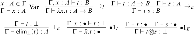

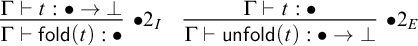


 Open access