


1. INTRODUCTION
The contribution from glaciers and ice sheets to sea-level rise is expected to continue over the next 100 years (Church and others, Reference Church2013). The current contribution of glaciers and ice caps to sea-level rise remains the highest at ~60% of the total contribution from all ice masses (Church and others, Reference Church2013). It is thus vital to fully comprehend how these smaller mountain glaciers and ice caps behave in order to produce more reliable predictions of glacier change in the future. Furthermore, by understanding the complex dynamics of smaller glaciers and ice caps we are able to model the large ice sheets more accurately. It is expected that the contribution from ice sheets to sea-level rise will increase significantly during the 21st (Century Rignot and others, Reference Rignot, van den Broeke, Monaghan and Lenaerts2011). In order to constrain these estimates, a better representation of glacier dynamics must be included in coupled ice-sheet models.
Observations of glacial systems are primarily at the glacier surface, even on relatively small glaciers. It is thus essential to determine the relationship between the measured surface properties and the corresponding englacial and subglacial conditions. Observations of glacier surfaces and velocities are becoming more frequent and detailed due to increased remote-sensing capabilities. These datasets allow for higher spatio-temporal coverage of glaciers. However, observations at the glacier bed remain limited. This is primarily due to the difficulty of accessing the bed of a glacier or ice sheet, which for the latter can be several thousands of metres deep. In most cases, access and measurements of basal conditions are only obtained through discrete boreholes that may take several seasons to drill. Engabreen is a unique location that is home to the Svartisen Subglacial Laboratory (SSL). Here scientists gain direct access to the ice/bed interface over a larger area than using a borehole, and at a fixed bedrock location. The physical access to the glacier bed allows scientists to directly measure the subglacial environment and use these observations to optimise model parameters. As a result, long time series of fundamental basal parameters, for example, subglacial pressure and basal sliding, have been measured (Lappegard and others, Reference Lappegard, Kohler, Jackson and Hagen2006; Lefeuvre and others, Reference Lefeuvre, Jackson, Lappegard and Hagen2015).
In this study, we combine both supraglacial and subglacial observations of the glacier with ice flow modelling to explore the subglacial conditions in the lower section of Engabreen. We are interested in how the conditions at the base evolve over the season as well as how much of the total velocity component is attributed to sliding. We model the 3-D flow of the glacier, constrained at the surface by satellite-based velocity fields from 2010 and 2014. We then invert for the basal friction parameter using the open-source finite element code, Elmer/Ice (Gagliardini and others, Reference Gagliardini2013), which has been used for similar studies e.g.: Schäfer and others (Reference Schäfer2012); Gillet-Chaulet and others (Reference Gillet-Chaulet2012); Gillet-Chaulet and others (Reference Gillet-Chaulet2016); Jay-Allemand and others (Reference Jay-Allemand, Gillet-Chaulet, Gagliardini and Nodet2011). The observations from the SSL constitute an important tool for calibrating the model setup and for interpreting our results.
2. SITE OVERVIEW
2.1. Engabreen
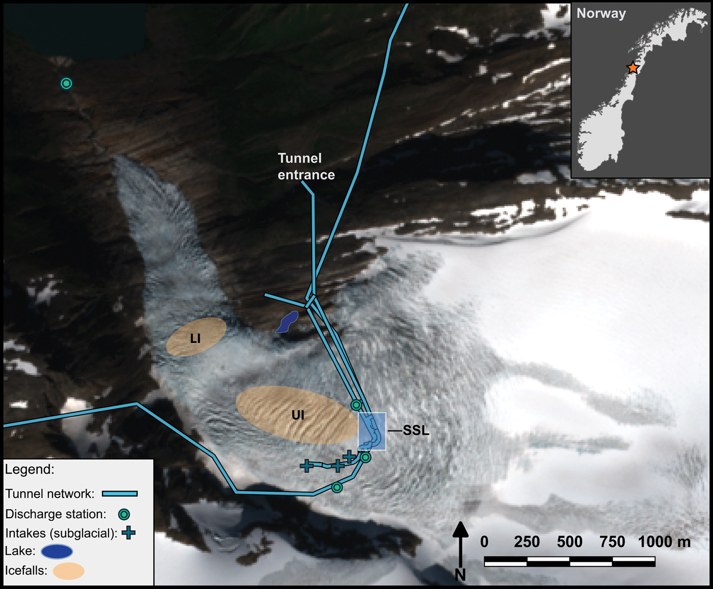
Engabreen is a temperate, maritime outlet glacier of the western Svartisen Ice Cap in Arctic Norway. It is a hard-bedded glacier underlain by gneiss and schist (Cohen and others, Reference Cohen2005). The glacier drainage basin initiates high up on a plateau in the accumulation zone of the Svartisen Ice Cap. The glacier then flows into a narrow valley where it enters an upper ice fall before making a right-angle bend. It then flows almost directly north and into a lower ice fall (Fig. 1). The glacier terminates in a thin ice tongue at ~100 m a.s.l. at the head of a deeply incised proglacial canyon (Fig. 1). The glacier has an elevation range of ~1500 m. Much of the bedrock geology around the margins of the glacier is punctuated by deep, cross-cutting faults lines, caused by the almost vertical strike of the rocks. The bedrock fault lines are perpendicular to the flow of ice for the downstream part below the bed (Fig. 1). The orientation of the fault lines in the upstream section of the glacier catchment (above the bend) is expected to be approximately parallel to the direction of the ice flow. While it is unknown exactly how these incised channels affect the glacier's drainage, it is likely that they play a role in routing the water from the margin into a more centralised channel that exits at the glacier terminus. This hypothesis is based on preliminary dye-tracing studies carried out in 2012 in a stream that flows out of the ice-marginal lake and back under the glacier in a narrow bedrock channel (Fig. 1), where 98% of the total injected dye was returned (Messerli, Reference Messerli2015).
Site overview of Engabreen and surrounding terrain. The two icefalls, labelled LI and UI, are referred to in the text as lower icefall and upper icefall, respectively. Background image is a 10 m resolution Sentinel-2 image from 20/07/2016 (Copernicus Sentinel data, 2016, processed by ESA).
The maritime climate at Engabreen ensures high accumulation rates in winter and extensive ablation in summer. Average annual temperature is measured at two weather stations around Engabreen. The air temperature measured at the discharge station at the proglacial lake (8 m a.s.l.) is ~5.5°C. The air temperature measured in the upper accumulation area of western Svartisen is ~−3.6°C, as measured at Skjæret, a nunatak located at 1364 m a.s.l. The summer mass balance at Engabreen ranges between −4.1 and −1.5 m w.e. and the winter mass balance between 1.2 and 4.1 m w.e for the period between 1970 and 2015 (Kjøllmoen and others, Reference Kjøllmoen, Andreassen, Elvehøy, Jackson and Giesen2011; Elvehøy, Reference Elvehøy2016). Average surface ice flow rates measured at Engabreen vary between 0.2 m d−1 at the margins and lower tongue and 0.7 m d−1 in the faster flowing central regions and the ice falls (Jackson and others, Reference Jackson, Brown and Elvehøy2005).
2.2. Subglacial environment
An extensive tunnel network exists beneath Engabreen, which was built as part of the Svartisen Hydroelectric power plant during the early 1990s. Water is extracted through numerous intakes, some of which exist directly at the base of the glacier as shown in Figure 1. The water is then routed through the subterranean tunnel network to a reservoir, Storglomvatnet, where it is fed into hydro-power turbines (Bogen and Bønsnes, Reference Bogen and Bønsnes2000). The subglacial intakes lie directly under the main trunk at Engabreen and were constructed in an area of low hydrological potential at the glacier bed (Kohler, Reference Kohler1998). The intakes further decrease the pressure at the glacier bed, driving water towards them. It is not known what effect the intakes have on the ice dynamics (Kohler, Reference Kohler1998), due to limited observations of the dynamics at Engabreen prior to the construction of the intakes. We consider it likely that the hydrological regime at Engabreen is reset due to the extraction of a large percentage of the water at the location of the intakes. The hydrological regime must re-establish and re-develop immediately downstream of the intakes, and is likely to be a more distributed system.
Integrated into the tunnel directly beneath Engabreen is the SSL (Kohler, Reference Kohler1998). The SSL is a series of research shafts that have been drilled into the bedrock to allow direct access to the glacier ice/rock interface. During winter months, access to the ice/bed interface is available by melting out a cave into the basal ice using hot water drilling.
Numerous studies have been, and continue to be carried out in the SSL in an attempt to further understand the subglacial environment (Cohen, Reference Cohen2000; Cohen and others, Reference Cohen, Hooke, Iverson and Kohler2000; Lappegard and others, Reference Lappegard, Kohler, Jackson and Hagen2006; Moore and others, Reference Moore2013; Lefeuvre and others, Reference Lefeuvre, Jackson, Lappegard and Hagen2015). These studies include hydrological investigations, sliding, subglacial pressure and basal ice characterisation. Current active measurements include basal pressure measurements using load cells, seismic geophones and several discharge measurements. As a result of the large hydropower development in the catchment, a substantial discharge station network exists both subglacially and proglacially, and provides us with a clear understanding of the hydrological cycle at Engabreen. Some of the main discharge stations are annotated in Figure 1. Many of these records and observations from the basal environment under Engabreen are applied in this to study to help constrain the ice flow model.
3. DATA
3.1. DEMs of surface elevation and bedrock
Laser scans of the glacier surface in 2001, 2008 and 2013 provide DEMs of the surface elevation for these years. The laser scan in 2013 (measured with a point density of 3.3 points m−2 using a Leica ALS70 airbourne laser scanner) only covers the glacier from slightly below the 1000 m contour, and it was, therefore, necessary to merge the 2013 DEM with the surface DEM from 2008 in order to get full coverage of the drainage basin. Differencing of the two DEMs shows elevation changes of up to 5–6 m a−1 near the glacier terminus, decreasing to <1 m a−1 around the 1000 m a.s.l. contour where the two DEMs were merged. The merged DEM for 2013 was smoothed using a Gaussian filter to remove small artefacts where the DEMs were joined (Fig. 2).
(a) The merged 2013 surface DEM. Contour spacing: 20 m. (b) RI-bedrock DEM: Bed topography constructed using radar measurements and ice-free topography. Contour spacing: 75 m. Red dots indicate the radar measurements described in Kennett and Laumann (Reference Kennett and Laumann1993). (c) RIF-Bedrock DEM: Bed topography constructed using radar measurements, ice-free topography and ice-flux derive thicknesses. Contour spacing: 75 m. Red dots indicate the radar measurements described in Kennett and Laumann (Reference Kennett and Laumann1993). (d)–(f) Three examples of ice velocities used in the study from three different satellite sensors: Landsat-8, TerraSAR-X and RADARSAT-2.
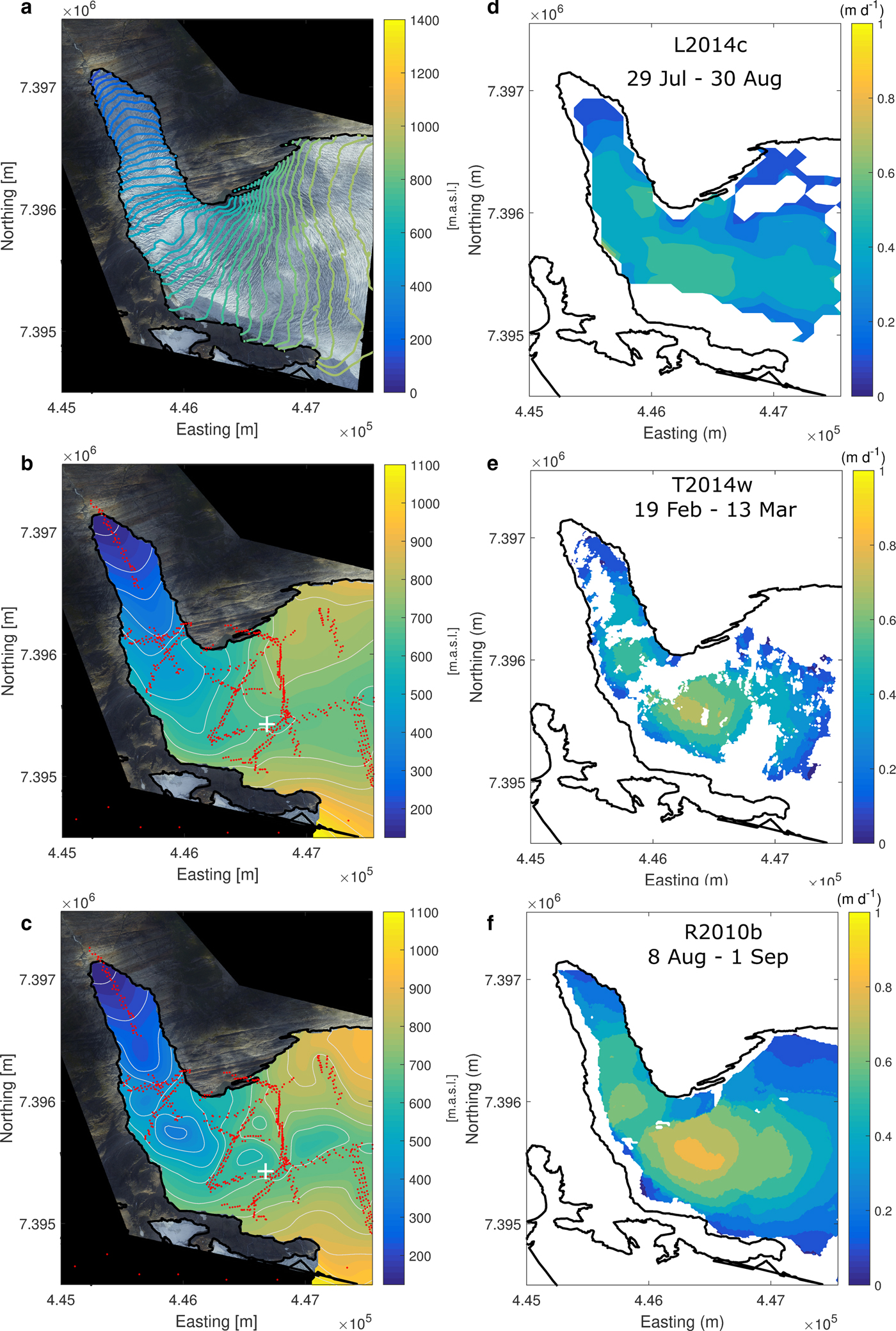
Ice thickness was measured in 1991 during an airbourne radar survey (Kennett and Laumann, Reference Kennett and Laumann1993). This is complemented by ground-based radar measurements of the bed from 1986 on upper Svartisen, and hot-water drilled boreholes on Engabreen from two campaigns in 1975 and 1987 (Kennett and Laumann, Reference Kennett and Laumann1993). A bedrock DEM was constructed using these radar data as well as the surrounding ice-free topography by fitting a smooth surface to the scattered data.
Some areas of Engabreen have sparse bedrock data-coverage, especially the upper elevation area of the glacier. We remedy this by filling in the larger areas without measurements using the ice-flux method described in Huss and Farinotti (Reference Huss and Farinotti2012). The method is based on mass conservation (i.e. changes in ice thickness over time is balanced by the mass balance and the ice divergence flux) and is thus not limited to glaciers in steady state. In its original form, it is applied to a global set of glaciers and thus a significant part of the input is parameterised. In this study, we can use direct observations as the input instead. The change in elevation over time is calculated using the 2001 and 2008 DEMs, and an elevation-dependent average mass balance is obtained using data reported to the WGMS (Andreassen and others, Reference Andreassen, Elvehøy, Jackson, Kjøllmoen and Giesen2011; WGMS, Reference Zemp, Nussbaumer, Naegeli, Gärtner-Roer, Paul, Hoelzle and Haeberli2013) for the same period. The average ice thickness is derived in 10m elevation bands using Glen's Flow Law and vertically integrated velocity, based on the assumption of parallel flow. The average ice thickness in each band is then re-distributed by applying a weighting-scheme depending on the distance to the nearest glacier boundary point and the local slope (Huss and Farinotti, Reference Huss and Farinotti2012) in order to get a 3-D DEM.
The ice thicknesses, derived from the flux method, are used to fill in the areas where radar data of bedrock elevation are sparse. The glacier is covered by a rectangular grid with a spacing of 25 m, and the distance from each grid point to the nearest radar measurement is calculated. The ice-flux derived value is assigned in instances where the distance between the grid points is >100 m. The two datasets are then combined and the interpolation scheme described above is applied to the combined dataset. Two DEMs are created, firstly the RI-bedrock DEM, which is based on the radar data and ice-free topography only; and secondly, the RIF-bedrock DEM which includes the ice-flux calculation in addition to the radar data and ice-free topography. These are contoured in Figures 2b, c, respectively.
Kennett and Laumann (Reference Kennett and Laumann1993) report that their measurements have an uncertainty of ±15 m, arising from the interpretation of the echograms and ±5 m antenna elevation. A further estimated ±7 m is reported, which is associated with a ±20 m uncertainty in the horizontal position. These three sources add up to ±27 m. The mean difference between the observed and modelled bedrock elevation (modelled-observed) in the area that we focus on in this paper is +25 m, which is within the uncertainty of the measurements. This agrees with a study of several Norwegian glaciers by Andreassen and others (Reference Andreassen, Huss, Melvold, Elvehøy and Winsvold2015), which shows that the flux method captures the overall thickness pattern.
The flux method also reveals locations of possible bedrock overdeepenings under the glacier tongue in areas not covered by radar data. Examples of these are at the bend, where the glacier turns north, and near the terminus (Fig. 2c). These predicted overdeepenings coincide with the compression of crevasses (Figs 1, 5) and a low surface slope. At the bend, there is, furthermore, a depression in the surface, indicating a low in the bedrock. Both versions of the bedrock DEM (the RIF-bedrock and the RI-bedrock) are applied in the inversion in order to give an idea of the robustness of the results to inaccuracies in the bedrock DEMs.
3.2. Ice velocity
Six ice velocity maps covering different periods in 2010 and 2014 are applied in this study. Examples of these are shown in Figures 2d–f. Further details and specifications of all velocity maps are given in Table 1.
Satellite data and processing parameters
3.2.1. Optical landsat velocity
Three velocity fields were produced by applying a normalised cross-correlation template matching algorithm to three Landsat-8 pairs using ImGRAFT (Messerli and Grinsted, Reference Messerli and Grinsted2015). From these six scenes, three independent velocity fields were generated covering the periods June, July and August 2014. The year 2014 was a particularly good year for optical data acquisition over the Svartisen area, which is a high elevation coastal region known for frequent cloud cover. Additionally, the Landsat acquisitions coincided with a planned winter TerraSAR-X acquisition over Svartisen. This enabled us to obtain close to an entire annual velocity coverage over the whole glacier.
A maximum surface flow speed of 1 m d−1 was measured in Engabreen's upper icefall. This implies that over a 16-day repeat orbit the maximum glacier displacement should be ~1 pixel, as Landsat's panchromatic band has a pixel resolution of 15 m × 15 m. It is, therefore, preferable to use a longer time window than 16 days in order to get a better signal-to-noise ratio and thereby reduce the error in the measurements. That said, we specifically chose velocity fields for the study with small/negligible bedrock motion. The bedrock motion provides us with a good estimation of the error in our velocity fields. The bedrock motion for Landsat pairs on flat, stable ground is small. The error estimate for both 16 and 32 day time intervals is up to 0.12 m d−1.
3.2.2. Synthetic aperture RADAR velocity
Three RADARSAT-2 Ultrafine scenes of Engabreen were acquired between July and September 2010. Additionally, two TerraSAR-X Spotlight scenes were acquired on 19 February and 13 March 2014. These data were then used to retrieve glacier surface velocity using the offset tracking method of the GAMMA software (Strozzi and others, Reference Strozzi, Luckman, Murray, Wegmuller and Werner2002). The size of the correlation matching window was adjusted according to the image resolution and expected maximum displacements during the repeat pass cycle. Velocity maps were then geocoded using the Norwegian DEM at 10 m resolution from the Norwegian mapping agency (kartverket.no). Velocities larger than the measured maximum were discarded and remaining mismatches were manually removed based on visual inspection of magnitude and direction of the velocity vectors.
4. MODEL
4.1. Forward model and set-up
The flow of ice is represented by the Stokes equations, and the full set of equations are solved by the Elmer/Ice model described in detail in (Gagliardini and others, Reference Gagliardini2013). The rheology of the ice is described by Glen's Flow Law, which relates the strain rate,  $\dot {\epsilon }_{ij}$, to the deviatoric stress, τ ij:
 $$ \dot{\epsilon}_{ij}=A\tau_{e}^{n-1}\tau_{ij}, \quad i,j=x,y,z $$
where τ e is the effective stress, which is proportional to the second invariant of the stress tensor, and n is the flow law exponent assumed to be 3. A is the creep parameter dependent on the physical and chemical properties of the ice. There is no general understanding of how they affect A (Cuffey and Paterson Reference Cuffey and Paterson2010), but ice temperature is best understood. We thus split A = E · A T(T), where A T depends on the temperature of the ice, T. Engabreen is a temperate glacier, and thus A T is assumed to have a constant value over the entire glacier domain. We apply A T = 2.4 · 10−24 s−1Pa−3, which is the value recommended in Cuffey and Paterson (Reference Cuffey and Paterson2010) for ice at the melting point. E is the enhancement factor, which is a parameter that takes into account the variations in strain rate. These variations are not otherwise accounted for in the equation, and E was originally introduced to explain the observed enhanced deformation of Pleistocene ice relative to the overlaying Holocene ice in ice sheets (Paterson, Reference Paterson1991). We do not expect Engabreen to contain pre-Holocene ice (Nesje and others, Reference Nesje, Bakke, Dahl, Lie and Matthews2008), but we expect that properties of the ice, such as impurity content and water content, will contribute to deviations from E = 1 (Cohen, Reference Cohen2000). Observed values of E range from 0.6 to >50 (Cuffey and Paterson, Reference Cuffey and Paterson2010). In this study, we use E as an empirical adjuster that is constant over the entire model domain. It is thus not a physical property of the ice, but by varying the value of E, we can investigate the effect of changing the ice viscosity in a simple manner. Using values of E > 1 will lower the viscosity i.e. soften the ice. We apply E = [1, 2, 3], and this choice of range will be discussed in section 5.
The ice surface is assumed to be stress-free. A no-melt condition and a simple friction law, locally linking the basal shear stress to the resulting sliding velocity via a spatially varying constant, are applied at the lower boundary:
 $${\bf \tau}_{\rm b} + \beta \cdot {\bf u}_{\rm b} = 0 $$
where τb and ub are the shear stress and basal velocity parallel to the bedrock, respectively, and β is the basal friction parameter. Higher values of β imply more friction/less sliding and vice versa.
The computation is done on an anisotropic mesh, produced from a regular mesh using the YAMS software (Frey and Alauzet, Reference Frey and Alauzet2005). This was first applied by Gillet-Chaulet and others (Reference Gillet-Chaulet2012), who refined the mesh based on the Hessian matrix of the observed velocity field in order to capture the flow features. The horizontal resolution of the mesh is 20m or more, and the initial 2-D footprint of the glacier is extruded to ten layers in the vertical.
4.2. Inverse model
We are interested in the spatial and temporal variation of the basal conditions. We apply the control inverse method (e.g. MacAyeal, Reference MacAyeal1993; Morlighem and others, Reference Morlighem2010; Gillet-Chaulet and others, Reference Gillet-Chaulet2012) implemented in Elmer/Ice (Gagliardini and others, Reference Gagliardini2013) using the observed surface velocity and elevation to infer the spatial distribution of the basal friction parameter, β.
The cost function that we want to minimise measures the mismatch between the observed, uHobs, and modelled, uHmod, horizontal velocities at the upper surface, Γs, of the glacier:
 $$ J_{o}=\int_{\Gamma_{\rm s}} {1\over 2} ( \vert {\bf u}_H{obs} \vert \displaystyle - \vert {\bf u}_H{mod}\displaystyle \vert )^2 \; {\rm d}\Gamma_{\rm s} $$
In order to avoid small wavelength variations in β, due to noise in the observations as well as to improve the conditioning of the inverse problem, we impose a Tikhonov regularisation term which penalises the first spatial derivative of β:
 $$ J_{reg}= {1 \over 2} \int_{\Gamma_{\rm b}}\left( \left({\partial \beta \over \partial x}\right)^2 + \left({\partial \beta \over \partial y}\right)^2 +\left({\partial \beta \over \partial z}\right)^2 \right) {\rm d}\Gamma_{\rm b} $$
where Γb is the base of the glacier. The total cost function that we want to minimise is thus:
 $$ J_{tot}=J_{\rm o} + \lambda J_{reg} $$
where λ is a positive ad hoc parameter, which we determine through L-curve analysis (Hansen, Reference Hansen2001). Minimising J tot will not provide the best fit to the observed surface-velocities, but a compromise between the fit to observations and the smoothness of β.
The ice velocity maps approximately cover the lower 30% of the drainage basin. In order to constrain the cost function on the slower moving upper part, we include velocity information from mass-balance stakes reported in Jackson and others (Reference Jackson, Brown and Elvehøy2005). These measurements indicate velocities that are predominantly <48 m a−1 and quickly decreasing to <25 m a−1 further upstream. These measurements are not from the same years as the satellite-derived fields, but we can use them to impose an upper limit on the velocity by dividing the uncovered area into bands with a maximum allowed velocity, uHmax. Thus, outside the satellite covered area, J o is then determined by Eqn (3) except with uHobs replaced with the maximum allowed velocity, uHmax, in the band for uHmod ≥ uHmax. We set J o = 0 when uHmod < uHmax.
5. EXPERIMENTS AND RESULTS
Table 2 contains a list of all the model experiments. It reflects the emphasis of the study on changes of the subglacial processes over the season and the sensitivity of the results to the choices of bedrock DEM and enhancement factor. We use measurements from the SSL of ice viscosity and basal sliding to constrain the value of the enhancement factor, E. In experiments that are forced using velocity fields from 2014, the merged 2013/2008 surface DEM is applied, and when forced using the 2010 velocity fields the 2008 DEM is applied.
Overview of the modelling experiments. The table includes: experiment name, choice of velocity field, choice of bedrock DEM, range of λ, which is tested and choice of enhancement factor E

5.1. Determining λ from L-curve analysis
L-curve analysis is a convenient way to display the trade-off between smoothing the optimised parameter (β in our case) to avoid fitting the solution to noise in the data, the J reg-term and the actual fit to data, the J o-term (e.g. Hansen, Reference Hansen2001) in Eqn (5). For some value of λ, the regularisation becomes too dominant and the misfit between the modelled and observed surface velocity fields grow (Hansen, Reference Hansen2001). Figure 3 shows the L-curves for the experiments using the R2010a velocity field, E = 2 and the two bedrock DEMs. The L-curves of the remaining experiments have a similar shape. The value of λ, for which the value of J o is smallest, varies little between experiments and in general it takes the value 108 when the RIF-bedrock DEM is applied and 109 for experiments using the RI-bedrock DEM.
L-curves of the experiments using the 2010a velocity field and E = 2. (a) Results using the RIF-bedrock DEM. (b) Results using the RI-bedrock DEM.

The L-curves show that the experiments using the RIF-bedrock DEM have a lower value of the cost-function overall (i.e. a smaller misfit between the modelled and observed velocity fields) compared with runs applying the RI-bedrock. The average difference between observed and modelled velocities over the domain is ~30% higher using the RI-bedrock compared with the RIF-bedrock DEM. For this reason, our discussion will mainly be based on results using the RIF-bedrock DEM.
Another general feature is the value of the cost-function, which increases with an increasing value of the enhancement factor, E, when the bedrock DEM is the same. Based on these results, E = 1 appears to be the best choice. However, the model only assimilates our knowledge of the surface velocity in the inversion. In the following, we will use measurements of basal sliding from the SSL to impose a further constraint following the inversion.
5.2. Enhancement factor
Basal ice rheology studies by Cohen (Reference Cohen2000) and Lappegard and others (Reference Lappegard, Kohler, Jackson and Hagen2006) at the SSL found values of the creep parameter, A, in the range of A = [1.5 · 10−23;1.5 · 10−22] Pa−3 s−1. These values are 6–60 times larger than that for clear, temperate ice as recommended in Cuffey and Paterson (Reference Cuffey and Paterson2010) which we ascribed to A T. The very soft basal ice is attributed to the higher sediment content of the basal ice and the high water content of the ice, including englacial water pockets (Jansson and others, Reference Jansson, Kohler and Pohjola1996). The measurements concern ice at the very base of Engabreen, and they are not representative as an average value for the entire ice column or for the glacier as a whole. Instead, these results suggest that Engabreen has a lower viscosity (i.e. is softer) than pure, crystalline ice and we must apply a value of E > 1.
Measurements of basal sliding at the SSL can help us constrain the upper limit of E in our setup. Basal sliding was measured at SSL during two field seasons in April 1996 and November 1997 by Cohen and others (Reference Cohen, Hooke, Iverson and Kohler2000) and in 2003 by Lappegard and others (Reference Lappegard, Kohler, Jackson and Hagen2006) and was found to be on the order of 10–15 cm d−1. As the measurements were performed either before or after the melt season, we use the winter map, T2014w, to calculate the fraction of sliding to total velocity. The average observed surface velocity over a 400 m×400 m area directly above the SSL using these data is ~50 cm d−1, and sliding thus amounts to ~20–30% of the surface velocity.
We can use this observation to constrain the value of E by comparing it to the ratio of modelled basal-to-surface velocity, ub/us, for each of the experiments using the T2014w velocity map. Increasing the value of the enhancement factor increases the deformational rate of the ice and thus shifts a larger proportion of the total velocity component from sliding to deformation. In the experiments using E = 1 and the T2014w velocity map, the ice is so stiff that the glacier downstream of the intakes essentially behaves as one slab of ice, with basal sliding accounting for the majority of the velocity i.e. plug flow (Nye, Reference Nye1951). In the area around the SSL, basal sliding accounts for ~78% of the total velocity when applying the RIF-bedrock DEM. Increasing the value of E to 2 or 3 makes the sliding more localised and reduces it to ~27% and ~10% of the total velocity in the SSL area, respectively. The specific sliding pattern depends on which of the two bedrock DEMs were used, but an appropriate value of the ratio of basal-to-surface velocity is reached when the value of E is in the range 2–3. We did not test values of E > 3 because this would lead to a further softening of the ice, and thus a lower value of ub/us than observed. E = 2 best fit the observations of sliding in the range of ~20–30% of the surface velocity in our model setup, and we focus the discussion of the results using this value.
The results discussed below are from experiments using E = 2 and the RIF-bedrock DEM. The overall pattern of β is not sensitive to the uncertainties in the bedrock DEM as was also concluded by Schäfer and others (Reference Schäfer2012). The features and trends that we highlight and discuss are evident in the majority of the experiments. Thus they are unlikely to be artefacts of our parameter choices, although they may vary in exact extent and magnitude.
Using the RIF-bedrock DEM and E = 2 as discussed above, the general discrepancies between observed and modelled surface velocities are predominantly <20% in the interior of the area covered by observations and larger at the margins. The largest discrepancies are found at the locations of the two icefalls (Fig. 1). Generally the model overestimates velocity by 20–40%, but can be up to 80% in a few localised areas. This is most likely related to the steep surface gradient adding to the uncertainty in the velocity maps as well as uncertainties in the bedrock DEM. Above the intakes, the model tends to underestimate the velocity between 0 and 20%. In general, the better spatial coverage provided by each map of observed surface velocity, the smaller the discrepancies.
5.3. Seasonal changes on different parts of the glacier
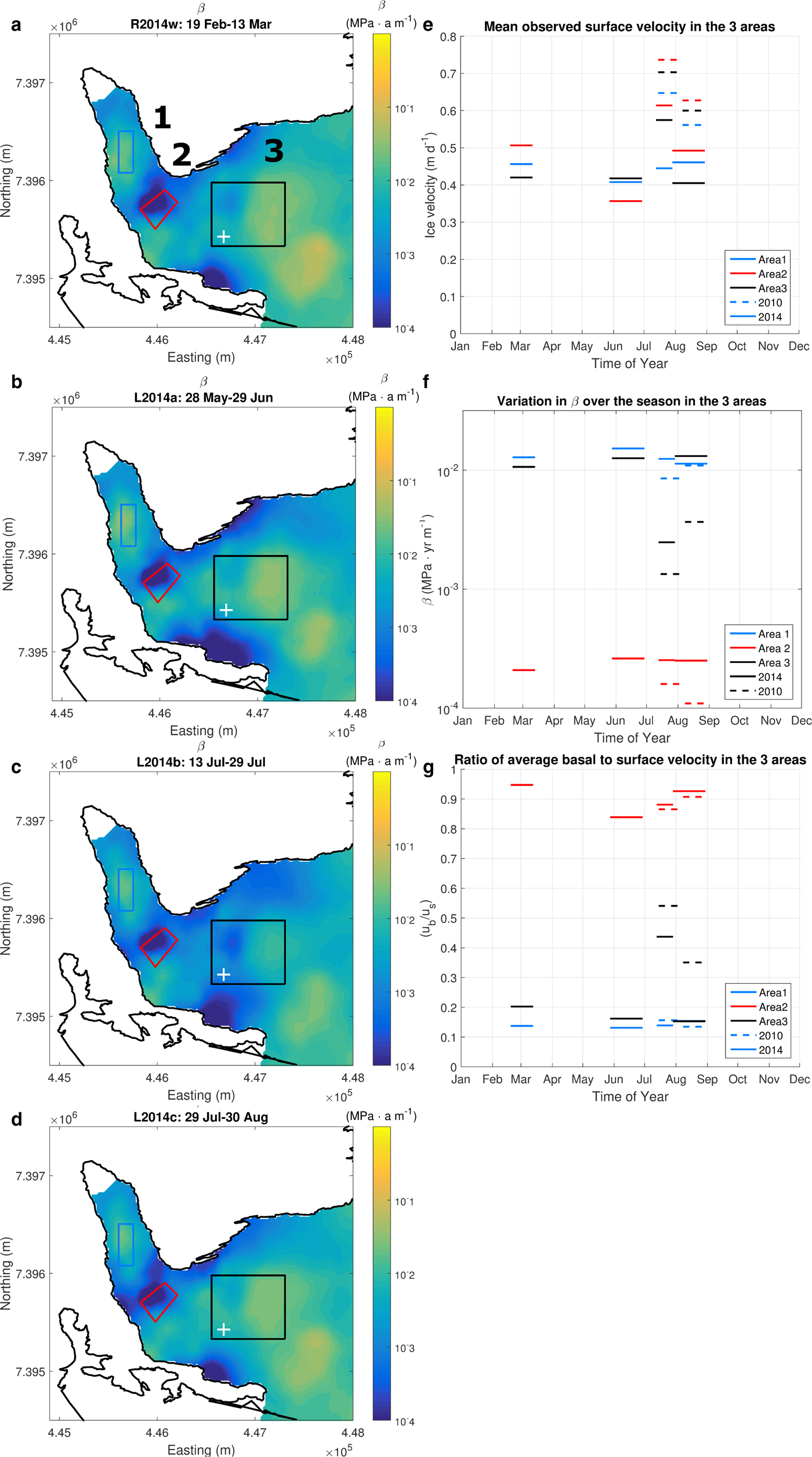
The variability of the basal conditions over the season is studied in three areas along the main flow of the glacier using the setup discussed above. See Figure 4 for the locations of the three areas. The location of Area 1 is chosen to investigate conditions close to the terminus of the glacier downstream of both icefalls. Area 2 covers the area just upstream of the lower icefall where there is a compression zone, which is visible in the optical image (Figures 1, 5). It also covers a large part of the overdeepening inferred by the flux-method. Area 3 is placed just above the intakes. This area is the largest of the three because we want to investigate how the basal conditions evolve over a larger area with less influence from small-scale features. The changes in the spatial distribution of the basal friction parameter, β, throughout 2014 is shown in the left-hand column of Figure 4. The right-hand side displays the observed surface velocity, the average β-value and the ratio of modelled basal-to-surface velocity, ub/us in each area for the six velocity fields (both 2010 and 2014 velocity fields). The results show that the areas vary in different ways over the season:
(a–d) The spatial distribution of the basal friction parameter, β, from the 2014 velocity fields. Blue colours indicate lower friction and yellow higher friction. The numbers 1, 2 and 3 show the three areas discussed in the text. The position of the white + marks the position of the intakes. (e) The observed average velocity in the three areas for both 2010 and 2014. (f) The average value of β in the three areas along the main flow path. (Note the logarithmic scale on the y-axis.) (g) The ratio of the modelled basal velocity to modelled surface velocity (ub/us) in the three areas.
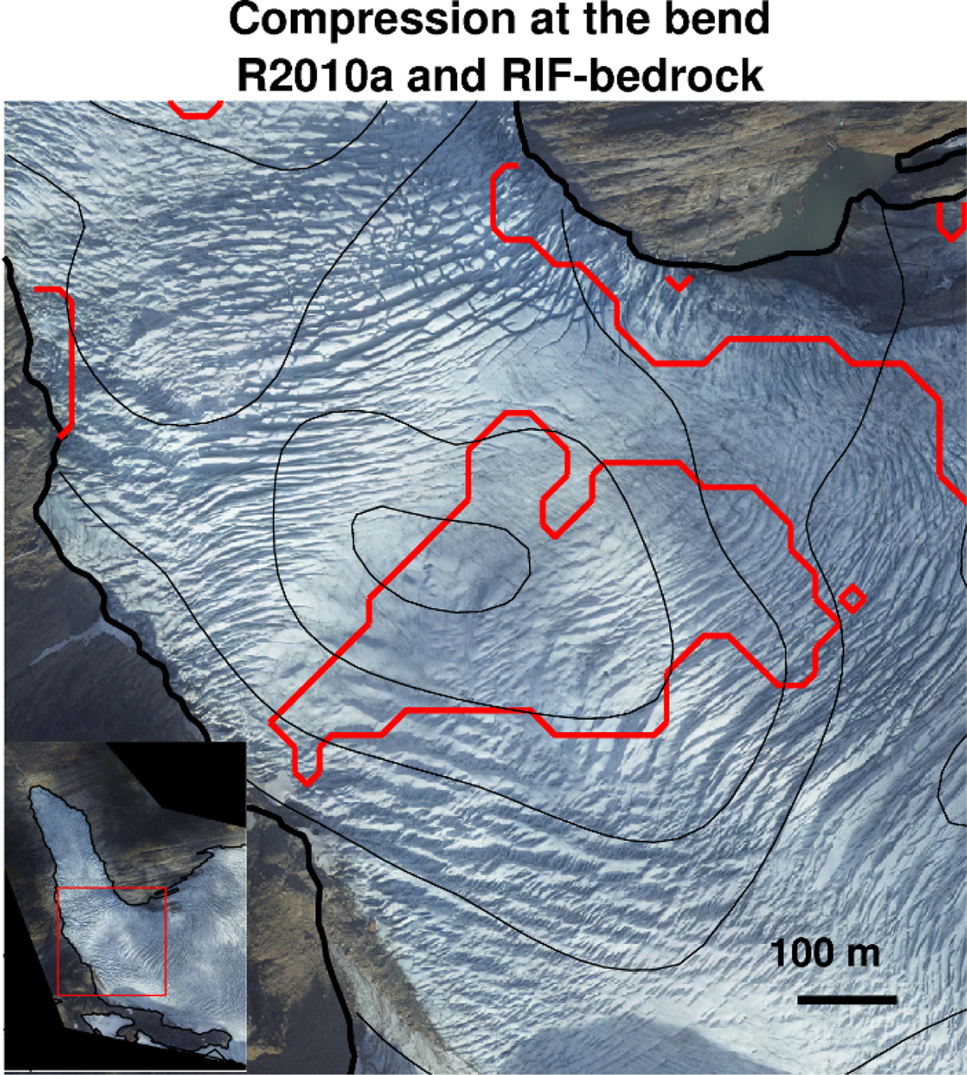
A compression zone is indicated by the closing of crevasses. The modelled surface eigenstresses also show a compression zone in the same location indicated by the thick red line. The exact location in the model depends mainly on the location and geometry of the overdeepening in the bedrock, but also on the velocity field that we try to assimilate. The uncertainties in the bedrock DEM thus influence this result. Bedrock contours in black with a contour interval of 75 m. Location of the close-up is shown in the inset.
Area 1 – The observed velocities show no clear seasonal signal. The 2014 velocity data exhibit only small variations over the year, while the 2010 data display a slow-down from July to August. The average modelled β-values thus also show no large variations. The ratio ub/us is <~0.2 in all experiments. However, we know from GPS measurements and time-lapse camera data with a higher temporal resolution that the velocity of this part of the glacier reacts over shorter timescales; such as in response to the onset of the melt season, other melt events and heavy rain falls (Messerli, Reference Messerli2015).
Area 2 – Observed velocities have a maximum in July in both the 2010 and 2014 data of 0.61 and 0.74 m d−1, respectively. However, this does not result in notable variations in β, most likely due to the already high value of ub/us and low β dominating the signal as given by the model. Sliding accounts for more than 80% of the total velocity in the model and does not vary significantly over the season. This area is a compression zone, as suggested by the closing of crevasses formed higher up the glacier (Fig. 5). This regime is captured by the model, showing an area with compressive stresses at the surface coinciding with the closing of crevasses. Our results exhibit significantly lower β-values than elsewhere on the glacier: the average values of β are 1–2 orders of magnitude lower than in Area 1 and Area 3. This is a feature common to all experiments. The area with low friction always extends from the inner part of the bend to at least mid-glacier, and often all the way across.
Area 3 – As is the case in Area 2, the maximum observed velocity is in July in both 2010 and 2014 with values of 0.57 and 0.70 m d−1, respectively. The opposite trend is seen in the β-values, with the lowest values modelled for July when the glacier speeds up, which indicates more sliding. The values increase again as it slows down. This trend is seen in the 2014 data as well as in the 2010 data. However, the drop in July is more significant in the 2014 results compared with the 2010 results. This is due to the overall faster surface velocities in the 2010 data. The modelled value of ub/us is consistently higher for the 2010 data, again due to faster velocities. Modelled values of the ratio for summer 2014 for the three available fields covering June, July and August are 0.16, 0.43 and 0.15, respectively. The values are 0.54 and 0.35 for the 2010 fields covering July and August, respectively.
Values of surface velocity, basal sliding, ub/us and the basal shear stress for Area 3 are tabulated in Table 3. They show how basal sliding and ub/us decrease with increasing E (softer ice) and how they vary other the season. For E > 1, ub/us increases by more than 75% from winter to its summer peak. The change is considerably smaller (33%) for E = 1, as ub is then already accounting for a large part of the total velocity.
Average values of modelled surface velocity (us [m a−1]), basal sliding (ub [m a−1]), the ratio of basal sliding to surface velocity u b/u s and the basal shear stress (τ b [kPa]) for area 3 (Fig. 4) for the 2014 winter velocity-field and the two fields from 2010 using the RIF-bedrock DEM
6. DISCUSSION
Based on our observations and modelling results, we discuss the differences in seasonality between the three areas on the glacier with a focus on the timing of the fastest velocities and the area with low basal friction (Area 2).
We observe maximum speeds in July for both Areas 2 and 3 in all our velocity data (both in 2010 and 2014). Messerli (Reference Messerli2015) observed the fastest velocity for Area 1 in May (not covered by our data). This is in connection with the onset of the melt season (spring event). During the spring event, the glacier speeds up in reaction to the sudden increase in englacial discharge to the bed, as the initial surface to bed connection is made. This influx of meltwater overwhelms the inefficient winter drainage configuration (Iken, Reference Iken1981; Iken and others, Reference Iken, Röthlisberger, Flotron and Haeberli1983; Mair and others, Reference Mair2003). Areas 2 and 3 lie at higher elevations than Area 1. One suggestion for the seeming delay in the speed-up of Areas 2 and 3 could be due to the upward migration of the spring event. However, observations and other studies suggest that the three areas all experience a spring event in May.
Previous velocity observations from time-lapse imagery of a region just downstream of Area 2 below the second icefall show that the spring-event is recorded simultaneously with Area 1 (Messerli, Reference Messerli2015). Due to the lack of high temporal-resolution velocity data in Areas 2 and 3, we are unable to confirm whether the spring event occurs at these elevations on the glacier in May. Nevertheless, a study by Lefeuvre and others (Reference Lefeuvre, Jackson, Lappegard and Hagen2015), using 20 years of basal pressure data, confirms a reconfiguration of the drainage system in May and a transition from inefficient to efficient drainage at the SSL (Area 3). However, the study suggests the evolution is relatively slow, on the order of days to weeks, maybe as a result of water storage in the snowpack. Indeed, satellite and time-lapse imagery of the area shows snow cover over Area 3 in May. It should be noted that the rate at which this transition from inefficient to efficient drainage occurs varies from year-to-year. This depends on the conditions at the glacier surface that affect the availability and supply of meltwater to the bed of the glacier. The conditions determining the water supply include temperature fluctuations, snow pack depth and precipitation type at the glacier surface.
The subglacial and proglacial hydrological records from the discharge stations (annotated in Fig. 1) indicate that there is potential for a spring event to occur in Area 3 simultaneously with the observed spring event in the lower elevation area. The hydrological records from the subglacial discharge stations correspond to both a rise in air temperatures to above freezing, and an increase in proglacial discharge. The subglacial and proglacial discharge hydrographs converge in June 2010. They continue to display similar discharge until they diverge again in October, where air temperatures begin to fall below zero at the elevation of Area 3. It is therefore likely that Areas 2 and 3 experience a period with increased flow and high velocities in May, which is not captured in our data.
From our velocity data, the fastest velocities in Areas 2 and 3 occur in July. This must relate to spatio-temporal differences in the morphology and structure of the subglacial drainage system, which are present at the time of the initial surface-to-bed hydrological connection. One clear difference between Areas 1 and 2 and Area 3 is the presence of subglacial intakes in Area 3. The intakes are observed to have a drainage efficiency between 40 and 90% depending on the time of year (Kohler, Reference Kohler1998). It was concluded from prior dye tracing studies that the intakes capture nearly all of the subglacial water in the area, thus depriving the area immediately downstream of water. This may cause a resetting of the drainage system in the region. The effect of such an abrupt change in the local hydrology has the potential to cause changes in the basal conditions. Kohler (Reference Kohler1998) suggests that the downstream drainage configuration changed from a predominantly channelised to a linked-cavity system after the subglacial intakes were established. Subglacial observations of the area immediately upstream of the intakes show a distinct channelised drainage system during the summer months (Kohler, Reference Kohler1998; Lappegard and others, Reference Lappegard, Kohler, Jackson and Hagen2006; Lefeuvre and others, Reference Lefeuvre, Jackson, Lappegard and Hagen2015).
Following the removal of the majority of the local subglacial discharge, it seems unlikely that enough water reaches the bed immediately downstream of the intakes to be able to sustain subglacial channels. The subglacial drainage system is more readily pressurised during periods of sudden increases in discharge as a result of the presence of a linked-cavity configuration. One hypothesis is that during periods of maximum bulk discharge (i.e. July), the intakes are unable to accommodate all the subglacial discharge, thus causing an overflow of the excess to the immediate downstream area. This additional delivery of water may lead to a temporary pressurisation (low effective pressure) of the underdeveloped linked-cavity configuration, leading to ice-bed separation and a speed-up in ice velocities (Iken, Reference Iken1981). This could explain the high velocities experienced in July in Area 2 (i.e. downstream of the intakes) and in Area 3 (i.e. directly above the intakes). Our model results show extensional flow immediately upstream and downstream of Area 3, which suggests that the areas are affect by longitudinal flow coupling. This is further supported by both the presence of clear crevasses in the upper icefall (Fig. 1), and a slight increase in the extensional flow in July indicated by the model. Simultaneously, Area 2 experiences a slight increase in compressional flow further supporting the notion of alterations in the effective pressure at the bed in reaction to changes in intake efficiency following maximum discharge in July.
Area 2, at the glacier bend, is different from elsewhere on the glacier due to the persistent low basal friction indicated by the low values of β in the model simulations. Basal sliding accounts for more than 80% of the total velocity component throughout the year. This could be due to low resistance at the bed compared with elsewhere on the glacier. Additionally, ice viscosity is not constant over the entire glacier as assumed using a spatially uniform value of A in our setup. In the latter case, the low friction is then an artefact of the ice being too stiff in that area in the model. Regardless, the conditions resulting in either low friction or lower viscosity must be present all year, or vary only slightly.
We argue in the following that the low basal friction inferred in the model is due to a combination of a slippery bed and softer ice at this particular location. Water at the base, either pooling in an overdeepening or saturating sediments in a bedrock depression, changes the basal conditions compared with elsewhere on the glacier. The flux-method predicts an overdeepening due to the low surface slope (Fig. 2) and is included in the RIF-bedrock DEM. Based on this, and the fact that there is a surface depression visible in the surface DEM (also visible in the aerial photograph, Fig. 5), provides supporting evidence for the presence of an overdeepening. At this location, there are no radar measurements of ice thickness available despite the airborne survey in 1991 covering this area (Kennett and Laumann, Reference Kennett and Laumann1993). It appears that some radar data have been removed from the dataset, possibly during an assessment of the data quality. However, a figure in Kennett and Laumann (Reference Kennett and Laumann1993) clearly shows a map of their contoured measurements, which includes a distinct bedrock low at the same location. There are numerous reasons that could lead to poor data quality, such as the presence of steep valley sides. If this were the case, we would assume this would affect all the measurements in the region. Radar waves are attenuated and scattered more by warmer ice with a high water content (Murray and others, Reference Murray, Stuart, Fry, Gamble and Crabtree2000; Matsuoka and others, Reference Matsuoka, MacGregor and Pattyn2012; MacGregor and others, Reference MacGregor2015). We find this a more likely explanation for the poor data quality in this area, as described in the following paragraphs.
The subglacial water paths (see Fig. 6) have been calculated using both bedrock DEMs and the 2008 and 2013 surface DEMs. The hydropotential is calculated at the overburden pressure and the water paths are assumed to follow the steepest gradient of the hydropotential (Shreve, Reference Shreve1972). In all combinations, there is a confluence of pathways in the low friction area. Furthermore, on the eastern side of the bend (see Fig. 1) there is a small lake that has recently emerged, which exists throughout the year and is dammed on the west side by ice. This lake formed in a depression where the ice has retreated. This indicates the ability to pool the available water in these depressions, and it is expected that a similar depression extends to the west under the glacier, located under the compression zone between the two icefalls as annotated in Figure 1.
(a) Waterpaths calculated using the RIF-bedrock DEM and 2008 surface (the other combinations of surfaces and bedrocks give similar results). Strain heating along the flowline (projection to horizontal plane marked in red) in the (b) R2010b_RIF_E2 experiment (note the increased strain heating internally in the ice at the bend) and (c) R2010b_RI_E2 experiment. The location of the overdeepening at the bend in the RIF-bedrock DEM is marked with a black X.
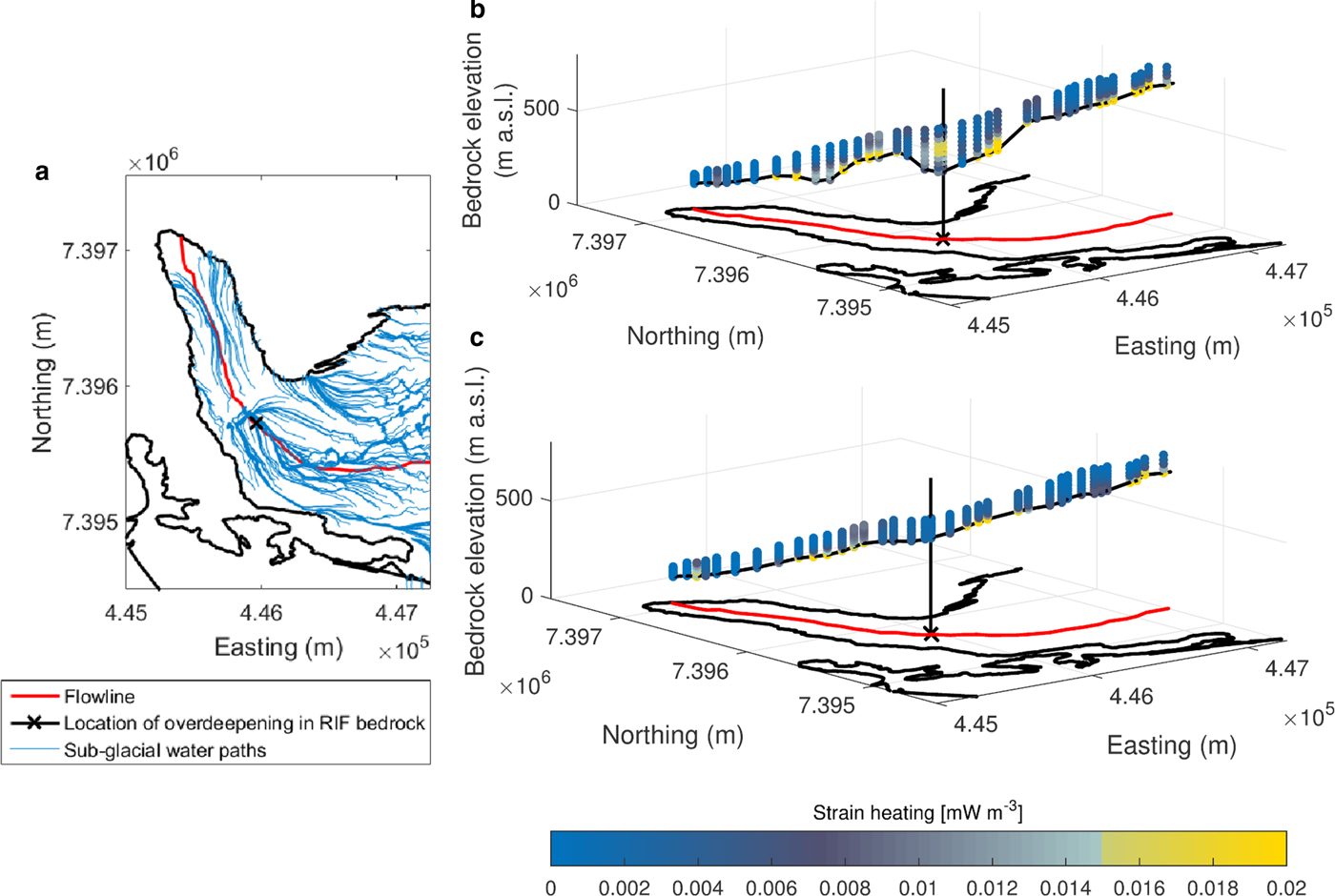
Engabreen is a temperate glacier, but the ice can soften further through increased impurity and water content as summarised in Cuffey and Paterson (Reference Cuffey and Paterson2010). The water content of the ice is high, and water pockets have been observed in the SSL. Increased strain heating can enhance the water content and thus further soften the ice. This is an important source of liquid water trapped in the ice of temperate glaciers (Aschwanden and Blatter, Reference Aschwanden and Blatter2005). Crevassing is another key process to lowering the viscosity of the ice through the delivery of meltwater to the bed and the fracturing/damage of the ice (e.g. Borstad and others, Reference Borstad2012; Colgan and others, Reference Colgan2015; Lüthi and others, Reference Lüthi2015). Meltwater has easy access to the lower part of the ice column through crevasses, where it can lower the viscosity through cryohydrologic warming and hydraulic weakening of the ice, as the meltwater refreezes and latent heat is released. Engabreen is highly crevassed in a large region upstream of Area 2 (Fig. 1). These processes, therefore, influence the flow over a larger region and are not specific to Area 2 with the low β-values. Strain heating calculated in the model is shown in an along flow cross-section of Engabreen in Figure 6. Strain heating is highest on the low elevation part of the glacier, where the ice coming from the plateau is funnelled into the narrow valley and takes a sharp northward turn. This is independent of bedrock DEM choice (Fig. 6), and in both cases there is a maximum in strain heating near the bedrock upstream of the bend.
In the experiments using the RIF-bedrock DEM, which includes the more pronounced overdeepening in the low friction area, there is an internal region above the overdeepening in the bedrock DEM of high strain heating (Fig. 6). This is not present using the RI-bedrock DEM. Thus, the presence of the overdeepening increases the strain heating. Whereas the overall β pattern is not very sensitive to the uncertainties in the bedrock DEM, the strain heating is much more dependent on the exact geometry. In general, the rougher RIF-bedrock DEM increases the stress and strain rates, and thus the strain heating, compared with the more smooth RI-bedrock DEM (Fig. 6). This is a source that is present year-round. We cannot conclude from our results whether the main cause of the modelled low-friction area is due to softer ice or slippery conditions at the bed, but there is evidence to support both and most likely it is a combination of the two.
7. CONCLUSIONS
We investigate basal conditions at Engabreen, Northern Norway, by inverting for the basal friction parameter using the full-Stokes model Elmer/Ice. Our study shows that there is a clear seasonal variation in the basal conditions around Area 3, which is upstream of the subglacial water intakes. Here the fraction of sliding to surface velocity more than doubles during summer compared with winter. This is most likely due to a peak in basal hydrological pressure, which is induced by overflow from the intakes. Our results reveal an overdeepening at the glacier bend, where modelled basal sliding accounts for more than 80% of the total velocity all year round. We propose that the ice can flow fast in this area due to a combination of water pooling at the base, and strain heating and damage which softens the ice. It is possible that we overestimate the amount of sliding at this location due to a local low in the ice viscosity not included in the model. Hence, our results show the importance of considering the spatial variability of the ice viscosity, which is influenced by variations in strain heating and debris content.
In our experiments, we have been fortunate to have measurements of basal sliding and viscosity from the SSL to help constrain our model setup. These observations show that Engabreen ice is soft due to the high englacial water content and debris-rich basal ice. They also show that the majority of the total velocity is due to internal deformation. We adjust the model setup to these observations and subsequently, test the sensitivity of our results to changes in viscosity through the spatially constant enhancement factor, E. We use E as an empirical adjuster to account for changes in viscosity relating to properties of the ice other than temperature. We find that our results of basal sliding and basal shear stress are very sensitive to the choice of E. When we decrease the viscosity (by increasing E to 2 or 3), we see a clear seasonal signal in the ratio of basal-to-surface velocity, with significant increases in the ratio during peak summer time. When E = 1, the fraction of basal-to-surface velocity is already high in winter (>60% in Area 3, just above the intakes and SSL). The changes over the seasons are then less dominant due to the stiffer ice. If we had not considered the observations from the SSL, we would have concluded that basal sliding accounts for most of the total velocity at Engabreen throughout the year. Instead, deformation constitutes the major velocity component outside the melt season. On glaciers where the total velocity is dominated by sliding, the modelled velocity is less sensitive to the viscosity of the ice (Schäfer and others, Reference Schäfer2012; Shapero and others, Reference Shapero, Joughin, Poinar, Morlighem and Gillet-Chaulet2016). For glaciers where deformation dominates the total velocity (such as Engabreen), our study emphasises the importance of applying the correct ice viscosity.
Access to the glacier bed, like at Engabreen, is rare. Although it is not possible to obtain glacier-specific deformational properties in every case, this study highlights the need for a greater range of deformation measurements from a wider variety of ice masses (e.g. maritime/continental, cold-based/warm-based). This would enable the categorisation and grouping of ice masses based on deformational properties, which are linked to their climatic, geographic and geological setting. This is a next step that is needed to better constrain ice flow models.
ACKNOWLEDGMENTS
We thank the editors and two anonymous reviewers for their helpful and constructive comments, which improved the manuscript considerably. This publication is contribution number 91 of the Nordic Centre of Excellence SVALI, Stability and Variations of Arctic Land Ice, funded by the Nordic Top-level Research Initiative (TRI). Anne Solgaard was supported by European Research Grant no. 246815 ‘Water Under the Ice’, GEUS and the Centre for Ice and Climate funded by the Danish National Research Foundation. Thomas Zwinger was supported by the Nordic Centre of Excellence, eSTICC. Miriam Jackson and Thomas Zwinger were supported by FP6 EC INTEGRAL project (Contract No. SST3-CT-2003-502845) and by the Nordic Centre of Excellence, SVALI. We also thank Statkraft for allowing access to the laboratory. Thomas Schellenberger was funded by the Research Council of Norway (RASTAR, 208013), the Norwegian Space Centre as part of European Space Agencys PRODEX program (C4000106033), and the European Union FP7 ERC project ICEMASS (320816). The TerraSAR-X and Radarsat-2 data were provided by Andreas Kääb through the German Aerospace Center DLR (LAN_0211) and NSC/KSAT under the Norwegian-Canadian Radarsat agreement. We thank Rune Juhl Jacobsen for help with the Elmer/Ice setup.


 Open access