


1. Introduction
In the central parts of polar ice sheets, ice is formed by a dry sintering process. At the transition from firn to ice, atmospheric air filling the interconnected pore space in the firn is isolated in bubbles. In cold ice the air is assumed to be well preserved. If air from old, well-dated ice samples is extracted and analyzed, the composition of atmospheric air from the past can be reconstructed. This method, which has been widely applied, is based on the assumptions that we can neglect: (1) air components dissolved or adsorbed on firn grains, (2) the fractionation processes during the enclosure of air in bubbles, and (3) the production of air components by chemical reactions in the ice. These assumptions must be tested for each air component and for each ice core. Such tests have been performed especially for the two important greenhouse gases, methane and carbon dioxide. Tests for methane showed no effects which alter the concentration significantly, but the CO2 situation is different.
Results from various polar ice cores from both hemispheres show that the atmospheric CO2 concentration increased steadily from about 280 ppmv in pre-industrial times (about 250 years ago) to about 315 ppmv in 1958 when direct and continuous measurements on atmospheric air started (Reference Neftel, Moor, Oeschger and StaufferNeftel and others, 1985; Reference Etheridge, Steele, Langenfelds, Francey, Barnola and MorganEtheridge and others, 1996). Different ice cores also show a significant increase in the atmospheric CO2 concentration from about 200 ppmv to 280 ppmv during the transition from the last glacial epoch to the Holocene (Reference Barnola, Raynaud, Korotkevich and LoriusBarnola and others, 1987; Reference Neftel, Oeschger, Staffelbach and StaufferNeftel and others, 1988; Reference Staffelbach, Neftel, Stauffer and JacobStaffelbach and others, 1991; Reference Raynaud, Jouzel, Barnola, Chappellaz, Delmas and LoriusRaynaud and others, 1993). These results can be considered reliable due to the very different conditions (annual temperature, accumulation rate, deposition of aerosols) at the various borehole locations. However, more detailed variations of the CO2 concentration measured on different ice cores do not agree with each other, and indicate that some of the assumptions mentioned above are not fulfilled for CO2.
The following differences have been observed:
CO2 records from various Greenland and Antarctic ice cores representing the last 300 years are in good agreement within the analytical and the dating uncertainties. But at the beginning of the second millennium AD, Greenland records show a CO2 concentration about 20 ppmv higher than Antarctic records. This is much more than could be explained by an interhemispheric gradient of the atmospheric CO2 concentration (Reference Barnola, Anklin, Porcheron, Raynaud, Schwander and StaufferBarnola and others, 1995).
The last glacial epoch was interrupted by numerous short interstadials, called Dansgaard/Oeschger events. Greenland records show CO2 concentrations during interstadials which are on average about 50–90 ppmv higher than during the stadials (Reference Stauffer, Hofer, Oeschger, Schwander and SiegenthalerStauffer and others, 1984; Reference Smith, Wahlen, Mastroianni, Taylor and MayewskiSmith and others, 1997b). Such high CO2 variations are missing in Antarctic ice cores (Reference Oeschger, Neftel, Staffelbach and StaufferOeschger and others, 1988).
Detailed analyses along ice cores show that the CO2 concentration in Greenland ice cores varies along certain core sections 60 ppmv or more within one or a few annual layers (Reference AnklinAnklin and others, 1997; Reference Smith, Wahlen, Mastroianni, Taylor and MayewskiSmith and others, 1997b). The scatter is especially high in Green land ice cores representing the last glacial epoch, though it is not restricted to these sections.
CO2 concentration records from Greenland ice cores are generally higher than those from Antarctic ice cores for the same time interval. However, there are some observations which show lower concentrations. Reference AnklinAnklin and others (1997) found values that were too low in the Greenland Ice Core Project (GRIP) ice core (compared with Antarctic records and other Greenland records) in the age range 7500–10 500 years BP. Reference Smith, Wahlen, Mastroianni and TaylorSmith and others (1997a) found values that were too low in a few samples from cold phases during the last glacial epoch.
CO2 is considerably enriched in melt layers due to the high solubility of CO2 in water (Reference Neftel, Oeschger, Schwander and StaufferNeftel and others, 1983), but an enrichment of CO2 in ice at Summit (mean annual air temperature −32°C) due to melt layers can be excluded for most of the observed high CO2 values. The fact that fast changes of CH4 concentrations which accompany Dansgaard/Oeschger events are observed in Greenland and Antarctica with about the same amplitude (Reference Stauffer, Hofer, Oeschger, Schwander and SiegenthalerStauffer and others, 1997) excludes the possibility that fast variations of the CO2 concentration are missing due to a strong attenuation in Antarctic records caused by much lower accumulation rates.
The most probable explanation for CO2 peak values in short core sections representing only a few annual layers or even less than an annual layer, especially in Greenland ice, is a production of CO2 by chemical reactions between impurities in the cold ice. Reference DelmasDelmas (1993) suggested acid–carbonate reactions for “well-delimited parts” of Greenland ice-core records. During the last ice age, the precipitation over Greenland was generally alkaline (Reference Meeker, Mayewski, Twickler, Whitlow and MeeseMeeker and others, 1997), but during Dansgaard/Oeschger events it was almost neutral. Delmas expected that thin acid and alkaline ice layers are mixed in core sections representing Dansgaard/Oeschger events and that the probability of an acid-carbonate reaction is much higher in such layers than in ice which is definitely acid or alkaline.
However, production of CO2 by acid–carbonate reaction is not limited to core sections representing Dansgaard/Oeschger events. Carbonate concentrations are found also in ice which is clearly acidic on average, as in Holocene Greenland ice (Reference FuhrerFuhrer, 1995). Carbonates are not the only carbon-containing compound, and CO2 can also be produced by the oxidation of organic material (Reference Raynaud, Jouzel, Barnola, Chappellaz, Delmas and LoriusRaynaud and others, 1993). For the oxidation reaction, an oxidant is needed; it could be hydrogen peroxide or an acid. Table 1 gives estimates of the mean concentrations of carbon in different compounds, and of hydrogen peroxide and of H+ in ice-age and Holocene ice from Greenland and Antarctica.
Estimated mean concentrations of typical compounds containing carbon, H2O2 and H+

The aim of this paper is to investigate what reactions can possibly produce CO2, and to assign CO2 peak values observed in short core sections to the most probable reactions. For this purpose we performed high-resolution chemical analyses for compounds containing carbon and possible reaction partners along short core sections which showed CO2 peak values.
2. Analytical Procedures
For measurements of CO2 concentration, the gases have to be recovered using a dry extraction method owing to the possible acid–carbonate reaction in the liquid phase if carbonates are present (Reference Anklin, Barnola, Schwander, Stauffer and RaynaudAnklin and others, 1995). A high extraction efficiency is needed to avoid artefacts by fractionation. But there are not yet any dry extraction techniques available that release >90% of the gas content (for bubble ice), and which are practicable with only 4–5 g of ice, as necessary to allow a high spatial resolution. To reveal a possible annual (non-atmospheric) variation of the CO2 concentration in the selected GRIP samples, a depth resolution of 15 mm or less is needed.
After crushing of the ice in a vacuum vessel at −33°C, the released gases expand through a cold trap to a laser absorption cell, where they are analyzed with an infrared laser absorption spectrometer. The laser wavelength is tuned several times over an absorption line of the CO2 molecule. The concentration is calibrated with the absorption of a standard gas at the same pressure as the sample and is the mean over all the tunings (six in general). CO2 standards added to artificial gas-free ice and then crushed and handled like normal samples show a reproducibility better than 1.3 ppmv (1 std dev. over all the standard measurements).
Measurements of the chemical species (H2O2, formaldehyde (HCHO), Ca2+ and the electrical conductivity of the melted sample) are done with a continuous flow analysis (CFA) system (Reference Fuhrer, Neftel, Anklin and MaggiFuhrer and others, 1993). No diffusion correction for the CFA data was applied. Therefore, the resolution is about the same as for the 15 mm long discrete samples for CO2. For all the correlation calculations, the different data records have been filtered using a spline (Reference EntingEnting, 1987) with a cut-off (half-amplitude) length for the variations of 15 mm depth to obtain continuous records.
Carbonate measurements have been done with a flow injection analysis (FIA) system on discrete samples. The technique is based on the high permeability of CO2 through silicon. Acid (0.5 M H3PO4) added to the molten sample transforms most of the carbonate to CO2(aq). This liquid flows along one side of a silicon membrane, with high-purity water as a receiver on the other side. CO2 transfers through the membrane. The conductivity of the receiver water is then measured. Calibration is done with different solutions of known carbonate content. Cross-sensitivity tests with all the major impurities in natural ice showed no signals above the detection limit (Reference FuhrerFuhrer, 1995). Prior to melting of the samples, the ice is milled to small fragments under CO2-free conditions. These fragments are then sieved (0.8 mm < diameter < 3 mm). This procedure was applied to release all the gaseous CO2 and to exclude the very fine powder that is easily contaminated. Measurements of real samples with carbonate contents under the detection limit prove that the gaseous CO2 was removed better than corresponding to a concentration of 20 ppmv.
To ensure parallel measurements, the samples were cut from one piece of ice. For chemical analysis with the CFA technique, a cross-section of 27 × 27 mm2 was used, whereas the discrete CO2 samples were cut just beside the CFA part with a size of 15 × 20 × 20 mm3.
The carbonate data are compared with earlier Ca2+ measurements (Reference Fuhrer, Neftel, Anklin and MaggiFuhrer and others, 1993) and with CO2 measurements made earlier and with a resolution of only 25 mm. Therefore, the accuracy for these two sections in depth is limited, and the different records may have an offset in depth of up to 50 mm.
3. Results
In Figures 1–5, high-resolution multi-parameter records from selected sections of the GRIP ice core are shown. Typical for all records are distinct peak values in the CO2 concentration. However, the amplitudes of the peaks are different. For the ice samples younger than 8000 years the surplus is in the range 15–25 ppmv, while for older samples it is >50 ppmv.
CO2, H2O2, HCHO, Ca+ and H+ concentrations along a section of the GRIP ice core, representing about two annual layers. Concentrations are given in μmol kg−1 ice. The proton concentration is calculated based on ECMs (Reference HammerHammer, 1980) (dashed line, left scale); the solid line shows the electrical conductivity of the meltwater (right scale). The CO2 concentration is given in ppmv (right scale) and the deviation from 282 ppmv in μmol kg−1 ice (left scale) assuming that the air content of the ice is 90 cm3 kg−1 ice.

CO2, H2O2, HCHO, Ca+ and H+ concentrations along a section of the GRIP ice core, representing about three annual layers. Concentrations are given in μmol kg−1 ice. The proton concentration is calculated based on ECMs (dashed line, left scale); the solid line shows the electrical conductivity of the meltwater (right scale). The CO2 concentration is given in ppmv (right scale) and the deviation from 278 ppmv in μmol kg−1 ice (left scale). The missing part is due to a break in the core.

CO2, carbonate, H2O2, HCHO, Ca+ and H+ concentrations along a section of the GRIP ice core, representing a little less than two annual layers. Concentrations are given in μmol kg−1 ice. The proton concentration is calculated based on ECMs. The CO2 concentration is given in ppmv (right scale), and the deviation from 277 ppmv in μmol kg−1 ice (left scale).

CO2, H2O2, HCHO, Ca+ and H+ concentrations along a section of the GRIP ice core, representing about four annual layers. Concentrations are given in μmol kg−1 ice. The proton concentration is calculated based on ECMs (dashed line, left scale). The solid line shows the electrical conductivity of the meltwater (right scale). The CO2 concentration is given in ppmv (right scale), and the deviation from 260 ppmv in μmol kg−1 ice (left scale).

CO2, carbonate, H2O2, HCHO, Ca+ and H+ concentrations along a section of the GRIP ice core, representing about ten annual layers. Concentrations are given in μmol kg−1 ice. The proton concentration is calculated based on ECMs. The CO2 concentration is given in ppmv (right scale), and the deviation from 245 ppmv in μmol kg−1 ice (left scale).

The measurement of the carbonate concentration is very difficult and laborious. Consequently, we have only two records available, and for one of these no H2O2 or HCHO measurements have been performed.
Figure 1 shows a core section about 1100 years old (Reference JohnsenJohnsen and others, 1992). The whole section represents about two annual layers. The measured CO2 concentrations are at least 5 ppmv higher than the atmospheric CO2 concentration at the time of ice formation (Reference IndermühleIndermühle and others, 1999) throughout the section. In addition, several samples at 265.97–266.03 m depth, and one sample at 266.06–266.08 m depth, show values about 20–30 ppmv higher. For this and the following record, no carbonate measurements are available. Therefore, the Ca2+ concentration must be taken as a proxy, assuming that on average about half of it is carbonate (CaCO3), as in Figure 5. We are aware that this is only a rough estimate and that the carbonate to calcium ratio varies with location and with climatic epoch. However, at present we have no better proxy available. The Ca2+ concentration is 0.05–0.4μmol kg−1 ice. In the region with elevated C02 values it is >0.07μmol kg−1. The electrical conductivity measurement (ECM) signal is >0.4 μS cm−1 (corresponding to an H+ concentration of about 1 μmol kg−1), indicating that acidity cannot be the limiting factor for an acid–carbonate reaction. Therefore, production of the CO2 surplus by an acid–carbonate reaction cannot be excluded. However, the course of the HCHO and H2O2 concentration suggests another possibility. The HCH0 concentration varies between 0.036 and 0.064 μmol kg−1, and the peak-to-peak difference of 0.028μmol kg−1 corresponds to only about 6 ppmv CO2 concentration, but HCH0 is only one of several organic compounds which could be oxidized. The drop of the oxidant H2O2 between 265.97 and 266.02 m depth is about 1.2μmol kg−1 ice. This corresponds to a possible CO2 surplus of 130 ppmv assuming the following net reaction: 2H2O2 + HCHO → 3H2O + CO2.
Figure 2 shows a record for a depth interval with an age of about 2100 years. It covers about three annual layers. The lowest CO2 values are around 280 ppmv, as expected for this time. There are elevated values, especially at 467.84– 467.88 and 467.96–468.03 m depth. Both elevated values correlate well with enriched calcium and acidity concentrations and with depleted formaldehyde and hydrogen peroxide concentrations. The acidity in both depth intervals (measured by ECM) is >0.3 μmol kg−1, and calcium shows a very high value, at least for the first CO2 peak. About 0.15 μmol carbonate per kg ice would be needed to produce the 30 ppmv higher CO2 concentrations. In this record there is also a remarkable anti-correlation between the CO2 concentrations and the HCHO and H2O2 concentrations. The drop of about 0.03μmol HCHO per kg ice corresponds to a CO2 concentration increase of 7 ppmv, so that again only part of the produced CO2 can originate from the oxidation of HCHO, while the depletion of H2O2 is on the order of 0.15 μmol kg−1 ice. We assume that additional short-chain organic species can be oxidized by H2O2.
Figure 3 shows a short depth interval representing ice which was formed about 2700 years ago. The record, which represents a little less than two annual layers, shows three samples with significantly elevated CO2 concentrations. The carbonate concentration is 0–0.15 μmol kg−1 ice (0.1μmol carbonate per kg ice can produce CO2 corresponding to about 25 ppmv) (Table 1). The calcium concentration is higher than the carbonate concentration in all parts of the core section except at 575.78–575.80 m where they are about equal. On average, only about one-quarter of the Ca2+ is present as calcium carbonate. There is an anticorrelation between calcium and carbonate concentration in this section. The conductivity is at least 0.3 μS cm−1 throughout the section, which implies a minimum H concentration of 0.85μmol kg−1 ice.
Figure 4 shows a depth interval from the early Holocene (about 8300 years BP). The 0.45 m interval represents about four annual layers. The mean atmospheric CO2 concentration for this time is around 260 ppmv (Reference IndermühleIndermuhle and others, 1999). Therefore, there are CO2 values in this record which are too high as well as too low. The acidity is very low at around 1351.08 m depth. The CO2 minimum at this depth could be due principally to a chemical depletion reaction (Smith, 1997a) in the ice, but more likely is a fractionation during extraction of the air. The depth interval is in the region where air bubbles disappear and air becomes enclosed into clathrates (Reference AnklinAnklin and others, 1997; Reference Stauffer, Tschumi and HondohStauffer and Tschumi, in press). The high CO2 values, on the other hand, can be explained by an acid–carbonate reaction or an oxidation of organic compounds (at least partly HCHO), as in the previous depth example, but there is no obvious correlation or anti-correlation between CO2 and any other measured compound.
The depth interval shown in Figure 5 represents ice from the end of the last glacial epoch (during the Younger Dryas cold period). The age of the ice is about 12 400 years BP, and the age of enclosed air is about 11 700 years BP. The figure includes about ten annual layers. Most samples show lower values than expected, again most probably due to a fractionation of CO2 between bubbles and clathrates. One sample shows an elevated CO2 concentration which correlates well with an elevated carbonate concentration of 12 μmol kg−1 ice. This amount of carbonate could produce CO2 corresponding to 3000 ppmv. The acidity shows a local minimum, but the H+ concentration is still on the order of 3 μmol kg−1 ice, having the potential to produce CO2 corresponding to 375 ppmv. Therefore, the observed CO2 surplus of 50 ppmv at 1650.80–1650.825 m depth could be produced by only 2% of the still available carbonate, and by 13% of the still available H+. The carbonate concentration is on average about half of the calcium concentration. There is a good correlation between the two compounds in this section. The two acidity minima correlate with two calcium maxima. The second calcium maximum is accompanied by a carbonate maximum, but no elevated CO2 concentration is observed in this depth interval. A CO2 record from the Greenland Ice Sheet Project II (GISP2) ice core covering the period of the Younger Dryas, which is characterized by low ECM signals and high calcium concentrations, shows CO2 concentrations of 244–288 ppmv (Reference Smith, Wahlen, Mastroianni and TaylorSmith and others, 1997a).
Figure 6 shows a record from the Byrd (Antarctica) ice core. Measurements along Antarctic ice cores generally show much smaller variations than those along Greenland cores. However, we selected an ice core from a depth range with surprisingly large variations. In the selected depth interval, representing about five annual layers, the CO2 concentration shows variations in a band between 240 and 280 ppmv. For this core section, only the conductivity measured on meltwater and no detailed ECMs are available, but comparison of the values provides good evidence that the ice is acidic. The calcium concentration is lower than in the Greenland ice cores. The HCHO concentration is low and its variations show no obvious correlation or anti-correlation with the measured CO2 concentration. The rather high concentrations and the strong variations of H2O2 are surprising for an Antarctic ice core.
CO2, H2O2, HCHO, Ca+ and H+ concentrations along a section of an ice core from Byrd station, representing about five annual layers. Concentrations are given in μmol kg−1 ice. No detailed ECMs are available for this core section. The solid line shows the electrical conductivity of the meltwater (right scale). The proton concentration was calculated from the meltwater conductivity assuming that only H+ is contributing to the electrical conductivity. The CO2 concentration is given in ppmv (right scale), and the deviation from 268 ppmv in μmol kg−1 ice (left scale).

4. Discussion and Interpretation of Results
There is strong evidence for chemical reactions in ice at temperatures as low as –32°C (as at the GRIP drilling site). Reference Sigg and NeftelSigg and Neftel (1991) observed chemical decomposition of H2O2. Thin layers of low H2O2 concentrations start to develop below the bubble close-off depth and become more frequent and broader with increasing depth. These “negative peaks” are observed where dust shows a maximum, and it has been concluded that H2O2 reacts with the dust (Reference Sigg and NeftelSigg and Neftel, 1991).
Comparison of the five records from the GRIP ice core and the one from Byrd station shows that it is not yet possible to attribute the CO2 surplus to production by a specific reaction, based on the detailed simultaneous measurements performed along the core sections. The production is most probably due to a combination of different reactions. The main reactions are certainly acid–carbonate reactions and the oxidation of organic compounds. For this second type of chemical reaction our measurements give information about only two possible source compounds; H2O2 is not the only possible oxidation reagent (e.g. sulphuric acid would also be one), and HCHO is just one of the most probable organic compounds which can be oxidized to CO2. However, correlation of the concentrations of the different species with the estimated CO2 surplus can give at least an idea which of the reaction types could be dominant.
In an attempt to quantify the contribution of possible reactions, we correlated the estimated CO2 surplus with the calcium, proton, hydrogen peroxide and formaldehyde concentrations. Table 2 gives the correlation coefficients between the different concentrations and the CO2 surplus for the four different core sections for which H2O2 and HCHO measurements are available. A multiple linear regression analysis increased the correlation coefficients only slightly, and significant coefficients were found only for HCHO and H2O2 in GRIP bags 484 and 851. These coefficients show that there is sufficient H2O2 and missing HCHO to explain the variance in CO2. Concerning the rather high correlation coefficient between HCHO and CO2 surplus in the core sections GRIP 484 and 851, it must be remembered that the observed HCHO depletion can explain only about 20% of the estimated CO2 surplus. However, HCHO is, as already mentioned, only one of several short-chain organic species which can produce CO and CO2 by oxidation (Reference Haan and RaynaudHaan and Raynaud, 1998). Detailed studies of organic materials trapped in polar ice are still limited. Light carboxylic acids like formate, acetate and oxalate have been measured in the GRIP core (Reference Legrand, De Angelis, Staffelbach, Neftel and StaufferLegrand and others, 1992) and in a shallow core from Dome Fuji (Reference WatanabeWatanabe and others, 1997). Fatty acids have been measured on several samples from Greenland and Antarctic ice cores (Reference Kawamura, Suzuki, Fujii and WatanabeKawamura and others, 1995; Reference Nishikiori, Kawamura and FujiiNishikiori and others, 1997). However, the resolution of these measurements does not allow a comparison with the highresolution CO2 records yet.
Correlation coefficients between measured CO2 concentrations and several compounds measured in parallel along short ice-core sections

The correlation between CO2 surplus and carbonates, Ca2+ and electrical conductivity is generally positive; the correlation between CO2 surplus and H2O2 and HCHO negative. We assume that:
Production from an acid–carbonate reaction is likely if CO2 peak values correlate with a local maximum of the carbonate and/or acid concentrations.
Production by the oxidation of organic compounds is likely if CO2 peak values correlate with a local depletion of the organic compound and/or the oxidation compound.
It is obvious that a reaction is more likely if the source compounds show a local maximum. Acidity, carbonates and calcium show seasonal variations (Reference Hammer, Oeschger and LangwayHammer, 1989; Reference Fuhrer, Neftel, Anklin and MaggiFuhrer and others, 1993). In most cases, the reaction of only a small fraction of the source compounds can explain qualitatively the CO2 surplus, so that elevated concentrations of the source compounds are expected even after a reaction. This justifies the first assumption.
Organic compounds and oxidants like HCHO and H2O2 show no seasonal variations in the Summit core below the firn–ice transition (Reference Sigg and NeftelSigg and Neftel, 1991). For H2O2, distinct minima develop with increasing depth. They are due to chemical reactions, as observed by Reference Sigg and NeftelSigg and Neftel (1991). Therefore, we expect H2O2 and HCHO to have a negative cor-relation with the measured CO2 concentration if the surplus is caused by a reaction between HCHO and H2O2.
So far, the carbonate-acidity reaction has been assumed to be the main candidate for CO2 production, especially in Greenland ice (Reference DelmasDelmas, 1993; Reference Smith, Wahlen, Mastroianni, Taylor and MayewskiSmith and others, 1997b). The good correlation between CO2 surpluses and the H2O2 and HCHO concentrations indicates that in the cases which we investigated, the oxidation of organic material is at least as important. This is supported by a surplus of the CO concentration in Greenland ice cores which cannot be produced by an acid–carbonate reaction (Reference Haan and RaynaudHaan and Raynaud, 1998). Isotope measurements could help to show whether oxidation of organic material or acid–carbonate reactions are dominant. Organic material has δ 13C values in the order of –25‰, while carbonate at its source region has high values of about 0‰. Relatively high δ 13C values of −4.45‰ and −3.7‰ have been found for the estimated CO2 surplus in Greenland samples representing the Last Glacial Maximum (Reference Smith, Wahlen, Mastroianni, Taylor and MayewskiSmith and others, 1997b), indicating an acid–carbonate reaction as a source, but low values of about −22‰ have been found in samples from the South Yamato (Antarctica) ice core representing an epoch during the last glaciation (Reference Machida, Nakazawa, Narita, Fujii, Aoki and WatanabeMachida and others, 1996) indicating an oxidation of organic material as a source. We conclude that in general, but not necessarily for mild epochs of Dansgaard/Oeschger events in Greenland ice, the oxidation of organic material is as important as acid–carbonate reactions for the production of CO2 in polar ice.
The correlation coefficients for the section of the Byrd ice core are completely different from those for the GRIP ice cores. They are smaller and a positive correlation is found between H2O2 and CO2 surplus, and a negative correlation between carbonate or calcium and CO2 surplus. The deviations of the measurements from the estimated correct value are smaller, as in Greenland cores, but still significant.
Can CO2 also be depleted by chemical reactions? In alkaline ice the reaction CO2 + H2O2 + CO3 2− → 2HCO3 − is possible in principle. Reference Smith, Wahlen, Mastroianni and TaylorSmith and others (1997a) assume that in a few samples from the GISP2 ice core representing ice from cold phases of the last glacial epoch, CO2 is depleted by this reaction. Measuring several adjacent samples along short sections of ice cores, we found in our laboratory mainly samples where CO2 has obviously been enriched, and only a few samples where it has clearly been depleted. Most of the latter are from a depth interval where bubbles are transformed into clathrates (1200–1700 m in the GRIP ice core) (Reference AnklinAnklin and others, 1997). The CO2 depletion in this zone is due to a fractionation of CO2 between bubbles and clathrates and a lower extraction efficiency for clathrates (Reference Stauffer, Tschumi and HondohStauffer and Tschumi, in press).
The fact that in most core sections carbonates, acidity, organic compounds and oxidizing reagents are still present after thousands of years (Table 1) demonstrates that the availability of the source compounds in the ice does not necessarily imply that a CO2-producing reaction occurs until a chemical equilibrium is reached. If it is assumed that both original compounds are distributed as single molecules independent of grain boundaries and veins, the reaction should depend only on the concentrations and on the diffusion constants of the two compounds in the ice. The reaction rate would be proportional to the probability that molecules from each source compound are coming close enough to react, which should be a monotonically decreasing function of time, mainly proportional to the product of the two concentrations.
However, one or both of the original reaction compounds can also be concentrated in dust grains, at grain boundaries or in veins, or formed along the edges where three ice crystals meet. There is some evidence that these veins consist of very narrow channels filled with a liquid eutectic mixture in which chemical reactions could occur (Reference Mulvaney, Wolff and OatesMulvaney and others, 1988; Reference Matsuoka, Fujita and MaeMatsuoka and others, 1997). One of the important open questions in ice-core research is whether each trace substance is equally distributed or is enriched at grain boundaries or in veins. Observations indicate that air bubbles are not concentrated along veins. For carbonates we assume that they are mainly present in dust grains and these are distributed on grain boundaries and in veins over the ice (Reference Alley, Perepezko and BentleyAlley and others, 1986a, b). Sulphuric acid is concentrated in veins (Reference Mulvaney, Wolff and OatesMulvaney and others, 1988), but chloride probably is not. There is no information available about the distribution of H2O2 and HCHO.
Grain boundaries and veins migrate through the ice due to crystal growth, and one can calculate the probability that a grain of a given size coincides with a grain boundary or a vein in a certain time interval. The fraction F(t) of ice that has passed a grain boundary at least once is estimated in the Appendix and shown in Figure 7a.
(a) Increase with time in the probability that uniformly distributed material in the ice will contact a grain boundary due to crystal growth F(t). After 1000 years about 82% of the material was in contact with a grain boundary. (b) Probability that an enclosure with radius rE = 5μm will contact a vein (triple junctions of grains) with radius rV = 0.4μm due to the movement of veins caused by crystal growth. After 3500 years, only about 0.6% of enclosures with radius rE have made contact with a vein.

The probability that the enclosure will contact not only a grain boundary but also a vein is much smaller and depends on enclosure radius r E and radius of the vein r V. The development of the probability with time for r E = 5μm and r V = 4μm is shown in Figure 7b.
The result of this very rough estimate can give only a qualitative explanation for the fact that only a few per cent of the compounds perform a chemical reaction if one of the compounds is present mainly in veins. For the oxidation of organic compounds, not even such a rough estimate of a reaction rate is possible because there is no information available about the distribution of H2O2, HCHO or any other organic compound in the ice.
5. Conclusions
Based on the results shown and discussed above, we draw the following conclusions:
CO2 can be produced by chemical reactions between impurities in cold polar ice.
The oxidation of organic compounds seems to be at least as important as acid–carbonate reactions for the production of CO2.
Depletion of CO2 by a chemical reaction is possible in principle, but we have not yet found any clear evidence for such depletion in our measurements in ice in which air is enclosed in bubbles. Depletions have been mainly found in the clathrate-formation zone where they are caused mainly by a fractionation of CO2 between bubbles and clathrates.
The atmospheric CO2 concentration has increased from about 280 ppmv at the beginning of industrialization to about 365 ppmv at present, and it increased during the transition from the last glacial epoch to the Holocene from about 200 ppmv to the pre-industrial concentration of 280 ppmv. These principal results of CO2 analyses on polar ice cores are not in doubt. They have been found in ice cores from various drilling sites with different accumulation rates and temperatures, and in ice with very different impurity concentrations.
Antarctic ice cores are generally more suitable for reconstruction of atmospheric CO2 concentration because they have lower impurity concentrations than Greenland ice cores. However, it should be noted that the dust concentration for the glacial epoch at Byrd station is comparable with the concentrations found in the GRIP ice core for the Holocene.
To identify the reaction responsible for a given CO2 surplus, further measurements are needed. Most important will be to investigate the distribution of different compounds in the ice. Very promising seem to be measurements of 13C/12C ratios on surplus CO2.
At present, the best way to ensure the reliability of CO2 measurements is to perform detailed measurements along a few annual layers. The scatter of the results should not be much higher than the reproducibility of the measurements (Reference StaufferStauffer and others, 1998; Reference IndermühleIndermuhle and others, 1999). A low carbonate concentration and a low H2O2 concentration in an ice core are advantageous.
Acknowledgements
This work was supported by the Swiss National Science Foundation and the “Bundesamt fur Energie”. We thank M. Hutterli, R. Röthlisberger and S. Sommer for performing the CFA, A. Fuhrer for the carbonate analyses and H. B. Clausen for unpublished detailed ECM records from the GRIP ice core.
Appendix
The fraction F(t) of ice which passes a grain boundary at least once can be calculated based on the following simplified assumptions:
The shape of the single crystals can be approximated by truncated octahedrons of uniform size with the length of an edge a and volume
 (Reference UnderwoodUnderwood, 1970).
Crystal growth is given during the first 3500 years (Reference Thorsteinsson, Kipfstuhl and MillerThorsteinsson and others, 1997) by
 , where D(t)2 is the mean area of a crystal in a thin section. The following values are valid for the GRIP site (Reference Thorsteinsson, Kipfstuhl and MillerThorsteinsson and others, 1997): D
0 = 1.6 mm at the firn–ice transition and k = 5.6 × 10⁻³ mm2a−1.
, where D(t)2 is the mean area of a crystal in a thin section. The following values are valid for the GRIP site (Reference Thorsteinsson, Kipfstuhl and MillerThorsteinsson and others, 1997): D
0 = 1.6 mm at the firn–ice transition and k = 5.6 × 10⁻³ mm2a−1.
The relation between the mean thin-section area D(t)2 and the edge a of the truncated octahedron is D(t)2 = 3.77a 2 (Reference UnderwoodUnderwood, 1970). This gives the following functions of volume and edge with time:
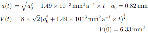
The fraction F(t) of the ice volume that has been passed at least once by a moving grain boundary is:

This fraction F(t) is identical with the probability that a homogeneously distributed small enclosure in the ice will contact a grain boundary within the time t. F(t) is shown in Figure 7a.



