Despite the important role played by intermediation in most markets, it is largely ignored by the standard theoretical literature. This is because a study of intermediation requires a basic model that describes explicitly the trade frictions that give rise to the function of intermediation. But this is missing from the standard market models, where the actual process of trading is left unmodeled.
Rubinstein and Wolinsky (Reference Rubinstein and Wolinsky1987)
1 Introduction
This Element surveys the theoretical economic literature on middlemen (i.e., intermediaries in the exchange process). This is relevant because, as is well recognized, intermediation plays a big role in many (if not most) markets for consumption goods, productive inputs, and assets, yet the activity is absent in standard general equilibrium theory. We present modern developments using search theory to study middlemen in markets with explicit frictions. The goal is not to discuss every paper in detail, but to develop a consistent framework that can be used to illustrate various models and ideas.Footnote 1
Starting with Rubinstein and Wolinsky (Reference Rubinstein and Wolinsky1987), this research builds models where intermediation emerges because certain agents have comparative advantages along some dimension. A general version of the Rubinstein–Wolinsky model is presented in Section 3, but here is an outline. There are consumers and producers of something called
 , plus other agents that neither consume nor produce
 , but potentially could act as middlemen by buying it from producers and selling it to consumers. In many (but not all) models agents meet bilaterally at random. In the original formulation, these other agents perform a middleman function when they have an advantage in search (i.e., they meet consumers faster than producers meet consumers).
Further studies generalize the framework’s technical specification by allowing different bargaining powers (in the original specification all agents have the same bargaining power); general populations (in the original the measures of buyers and sellers are the same); endogenous entry (participation is fixed in the original); production, search, and storage costs (these are absent from the original model); goods that are divisible (goods are indivisible in the original); and payment frictions (the original has transferable utility).
Further studies also explore different assumptions about the kinds of advantage middlemen might have, including superior information that lets them better recognize quality, a technology that lets them hold larger or more diverse inventories, and a superior ability to better enforce debt repayment. A main goal is to characterize the set of parameters consistent with the existence of equilibria with active intermediaries. Papers also investigate whether there is uniqueness or multiplicity of equilibria, as well as how intermediation affects efficiency. They also analyze if it attenuates or accentuates volatility. Of particular interest is finding conditions under which there emerge different patterns of exchange – only direct trade, only indirect trade, or both. Some papers also consider how multiple middlemen enter into intermediation chains. We review all of these in what follows.
While this Element mainly concerns theory, some facts help the motivation. In an early contribution, Spulber (Reference Spulber1996a) documented that intermediated exchange accounted for over 25% of GDP in the US in 1993, including retail trade (9.33%), wholesale trade (6.51%), finance/insurance (7.28%), and selected services (1.89%). Updating this from 1993 to 2025, 25% increased to 35.1% (BEA, US Department of Commerce, Federal Reserve Bank of St. Louis). For food, from 1993 to 2023, the share of dollars going to farmers and manufacturers declined from about 34% to 29%, while the share going to wholesale (distribution), retailing (supermarkets and grocery stores), and food services (restaurants, cafeterias, etc.) rose from 48% to 58% (USDA ERS Food Dollar Series). Switching from food to drink, in 2017 direct-to-consumer wine sales in the US were around 10% of the market, with the rest accounted for by retailers (Rhodes et al. Reference Rhodes, Watanabe and Zhou2021). In real estate, intermediated trade accounts for 91% of sales. In the labor market, recruitment and staffing firms account for two-thirds of all postings and attract most of the applications (Davis and de la Parra Reference Davis and de la Parra2025).
Philippon (Reference Philippon2015) discusses the share of financial intermediation in GDP and how it changes over time. As Lagos and Rocheteau (Reference Lagos and Rocheteau2006) report, different asset markets feature different microstructures – that is, while intermediated trade in the fed funds market is about 40%, NASDAQ is closer to 100%, and many OTC (over-the-counter) markets are in between, including markets for corporate, municipal, and emerging-market debt. In international trade, the impact of intermediation shows up in various ways, such as the fact that in the US wholesale and retail firms account for approximately 11% and 24% of exports and imports (Bernard et al. Reference Bernard, Jensen, Redding and Schott2007). The use of intermediary firms is especially important in developing economies, especially in Asia – for example, in the 1980s 300 trading (nonmanufacturing) Japanese firms accounted for 80% of trade (Rossman Reference Rossman1984).
In China today, Ahn et al. (Reference Ahn, Khandelwal and Wei2011) show 22% of exports are handled by intermediaries. In firm-level data, they also show that small or less productive firms rely disproportionately on intermediaries to access foreign markets. Those firms using intermediaries are significantly more likely to eventually become direct exporters, implying intermediaries lower entry barriers and boost overall trade. In the used-car market, Biglaiser et al. (Reference Biglaiser, Li, Murry and Zhao2020) document that dealer-mediated transactions command a consistent price premium over private sales, especially for older vehicles, and that cars sold through dealers exhibit higher quality. Together, all these findings demonstrate that middlemen can affect both the quantity and the quality of trade, and that suggests they are worth studying seriously.
Monieson (Reference Monieson2010) provides historical perspective on middlemen. While there are many interesting facets of this history that could be mentioned, one issue going back a long way is this: Do they provide a useful service, or simply profit from buying low and selling high? An extreme view is epitomized by Benjamin Disraeli, who said “It is well-known what a middleman is: he is a man who bamboozles one party and plunders the other.”Footnote 2 An alternative possibility is that they facilitate the process of exchange, which can enhance efficiency and welfare. As Ayn Rand (1971, p. 313) put it, “The shortest distance between two points is not a straight line – it’s a middleman.”Footnote 3
Reality may be somewhere between these extremes. While theory alone does not definitively resolve this debate, modeling intermediated trade formally in economic theory helps us understand the relevant factors. Before getting into formal models, we offer this story from Turner (Reference Turner1836, pp. 115–16), quoting a source from the eleventh century on the practice of buying low and selling high:
In the Saxon dialogues, the merchant (mancgere) is introduced: “I say that I am useful to the king, and to ealdormen, and to the rich, and to all people. I ascend my ship with my merchandise, and sail over the sea-like places, and sell my things, and buy dear things which are not produced in this land, and I bring them to you here with great danger over the sea; and sometimes I suffer shipwreck, with the loss of all my things, scarcely escaping myself.”
“What things do you bring to us?”
“Skins, silks, costly gems, and gold; various garments, pigment, wine, oil, ivory, and orichalcus, copper, and tin, silver, glass, and suchlike.”
“Will you sell your things here as you brought them here?”
“I will not, because what would my labour benefit me? I will sell them dearer here than I bought them there, that I may get some profit, to feed me, my wife, and children.”
The rest of the Element is organized as follows. Section 2 presents a rudimentary environment by way of introducing some basic terminology, notation, and ideas. Section 3 extends this to a generalization of the environment in Rubinstein–Wolinsky. Section 4 considers alternative assumptions and analyzes the possibility of multiple equilibria and endogenous dynamics. Sections 5 and 6 discuss information frictions and intermediation chains. Section 7 considers papers on inventories and directed rather than random search, while Section 8 summarizes some work focusing on OTC asset markets. Section 9 focuses on the relationship between middlemen, money, and credit. Section 10 mentions papers that do not fit elsewhere in the Element but are still relevant. Section 11 concludes.
2 A Simple Model
Before discussing the literature, it is useful to construct a simple two-period model that captures some of the main ideas, and, in particular, provides a clean version of the classic result in Rubinstein and Wolinsky (Reference Rubinstein and Wolinsky1987). It also lets us introduce notation, labeling, etcetera.
There are three agents – a producer
 , a middleman
 , and a consumer
 – that are interested in trading an indivisible good
 . The producer
 produces one unit of
 at cost
 , which we set to zero for now (for some applications it is better to think of
 as being endowed with
 ). The consumer
 derives utility
 from consuming one unit (for some applications it is better to think of
 as an input or asset and
 as
as
 ’s profit or return to acquiring it). The middleman
 neither produces nor consumes
 , but could acquire it from
 and resell it to
 ; that is intermediated trade.
There are two periods, or stages, to the trading process, with
 indifferent between getting
 in the first or second stage. Trade is bilateral, with the terms of trade determined here by generalized Nash bargaining, where the share of agent
 when bargaining with
 is denoted
 . There is at most one meeting per period, and the probability agent
 meets agent
 in each period is
 , or equivalently
 , by the bilateral nature of meetings. For now the
 ’s are parameters; later, they come from an underlying meeting technology. If
 meets
meets
 in the first stage, they trade, and the game is over. What is to be determined: Do
 and
and
 trade if they meet in the first stage?
Let there be returns to holding
 for
for
 and
and
 in the second stage, denoted
 and
and
 , where
 stands for storage costs in goods markets, while
 stands for dividends in asset markets. For now we assume
 (but see Section 4), with the cost incurred between the first and second stage, so it is sunk when
 or
or
 with
with
 meets
meets
 in stage 2. In addition to
 , there is a second tradable object,
 , that is divisible and serves as a payment instrument. The most generous way to think about this is the following: Any agent can produce or consume
 at constant marginal cost, or constant marginal utility, both normalized to
 , and when
 acquires
 from
from
 , the former makes a payment
 that increases
 ’s payoff and decreases
 ’s payoff by the same amount.
This way of sharing the trade surplus, using
 as a means of payment, is essentially what is usually called transferable utility. Our interpretation is generous in the sense that the direct transfer of utility is problematic. Consider Binmore (Reference Binmore and Health1992):
Sometimes it is assumed that contracts can be written that specify that some utils are to be transferred from one player to another
 Alert readers will be suspicious about such transfers
 Utils are not real objects and so cannot really be transferred; only physical commodities can actually be exchanged. Transferable utility therefore only makes proper sense in special cases. The leading case is that in which both players are risk-neutral and their von Neumann and Morgenstern utility scales have been chosen so that their utility from a sum of money
 [in our notation,
 ] is simply
 [in our notation,
 ]. Transferring one util from one player to another is then just the same as transferring one dollar.
We agree that “Utils are not real objects and so cannot really be transferred,” although we are less sure that “only physical commodities can actually be exchanged” since it seems clear that, for example, information or ideas can also be exchanged. A bigger issue concerns the claim that transferable utility is the same as paying with money. In serious monetary models, agents have a value function, or indirect utility function, over money holdings, but it is not generally linear (see surveys by Lagos et al. Reference Lagos, Rocheteau and Wright2017 and Rocheteau and Nosal Reference Rocheteau and Nosal2017). Well, in some models, sometimes money actually does enter linearly but up to a point, which does not correspond to transferable utility for the simple reason that buyers tend to run out of money, while in transferable utility models they never run out of utils.
Therefore, instead of pretending that
 is money, it is better to say there is a good
 that anyone can consume and produce. This avoids Binmore’s justified complaint about utils being transferred without doing a disservice to monetary/payment economics. At the risk of sounding pedantic, we emphasize this because work in the area is concerned with microfoundations, so it is important to think through such details, although we try not to dwell on it too much in what follows.
So, when
 changes hands,
 pays
pays
 to
to
 ,
,
 pays
pays
 to
to
 , and
, and
 pays
pays
 to
to
 . Interpreting these as prices, we call
 the direct price,
 the wholesale price, and
 the retail price. However, this is not as obvious as it may appear. First, if
 is divisible, and endogenous, as it is in some of the models presented in Sections 5, 7, and 9, in principle it might be better to call
 the price. Having said that, in practice it could be that we see (in the data)
 but not
 , which is especially relevant when
 corresponds to quality rather than quantity. Second, while
 is the price of
 in terms of
 , it makes as much sense to say
 is the price of
 in terms of
 .
.
In standard usage the price refers to the amount of money a buyer pays to get
 , which is hard to understand in models without money. Indeed, without money changing hands, it is not at all clear who is the buyer and who is the seller, any more than those labels make sense when
 gives
gives
 apples in trade for bananas. This may or may not matter, depending on context (see Wright and Wong Reference Wright and Wong2014 for an extended discussion). In any case, if we call the
 s prices, there arise several other interesting variables, like the spread
 and markup
 .
.
In the first period,
 is assumed to produce
 before meetings occur. If
 meets
meets
 they always trade, as mentioned. If
 meets no one, or
 meets
meets
 and they decide not to trade,
 and
and
 proceed to stage 2, while
 is assumed to drop out, which, by assumption, does not affect the probability
 and
and
 meet. If
 meets
meets
 and they trade,
 and
and
 proceed to stage 2 while
 drops out, since, by assumption,
 can only produce once here. Note that in a stage 1 meeting,
 and
and
 can differ along three dimensions:
 , their probability of meeting
 in stage 2;
 , their bargaining power; and
 , their return to holding
 , which for the purposes of this discussion satisfies
 (but see Section 4).
Let
 ,
,
 , and
, and
 be the value functions of
 ,
,
 , and
, and
 in the second stage. Then, the surpluses
 when
when
 trades with
 , using the labels direct, retail, and wholesale suggested earlier, are:
 (1)
(1)
 (2)
(2)
 (3)
(3)
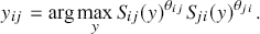
In each trade
 solves the bargaining problem
 (4)
(4)
However, with transferable utility (in the sense discussed earlier, where
 produces and
 consumes it with equal marginal cost and utility), the bargaining protocol, as long as it is reasonable, does not matter. So, we simply say
 gets a share
 of total surplus
 , which leads to
 (5)
(5)
Let the probability
 and
and
 trade at stage 1 be
 . Then the second-stage value functions are
 (6)
(6)
 (7)
(7)
 (8)
(8)
In other words, these values are the product of meeting probabilities and surpluses, minus storage cost. Note that for now it is taken for granted that all agents participate in the market, but that will be checked in Section 3.
Then, after inserting the
 s and
s and
 s, we have
 (9)
(9)
 (10)
(10)
 (11)
(11)
Note that
 and
and
 do not enter the second stage simultaneously. At least one of
 or
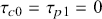
or
 is an off-equilibrium value. Nonetheless, we need to track both in order to determine
 , the probability of wholesale trade. Here
 only depends on the sign of the total surplus
 ; that is, whether there are gains from trade between
 and
and
 . What we call the best response conditions are then:
 (12)
(12)
When all agents participate,
 is the only decision. Thus, an equilibrium is given by
 ’s and
 satisfying (9)–(12), from which other variables, like the
 s, are easily determined.
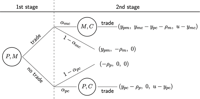
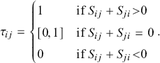
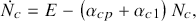
Figure 1 shows the structure of the model. It is easy to see that equilibrium exists and is unique. Letting
 , in equilibrium
 if
if
 and
and
 if
if
 .Footnote 4 Intuitively,
 means
means
 is active, intermediating by buying
 from
from
 and selling it to
 , if and only if
 has some advantage over
 . This in general means
 has some combination of being better at search,
 , or bargaining,
 , or storage,
 . Although their environment is more complicated in some ways, Rubinstein–Wolinsky (Reference Rubinstein and Wolinsky1987) is, in our notation, the special case where
 and
and
 , which gives their classic result:
 is active if and only if
 . More generally,
 can be fundamentally inferior to
 in terms of search or storage,
 or
or
 , and equilibrium can still have
 , if
, if
 has an advantage over
 squeezing surplus out of
 , which looks like inefficient rent-seeking activity.
Structure of the simple model.
To be precise, we can measure welfare by the sum of the
 s, which equals the expected utility of
 minus the cost of
 or
or
 delivering the goods. The optimal wholesale trade maximizes welfare:

Letting
 , it follows that
 if
if
 and
and
 otherwise. Note that
 depends on the
 s while
 does not. Given
 and
and
 , we can evaluate when equilibrium is efficient. In the special Rubinstein–Wolinsky (Reference Rubinstein and Wolinsky1987) case,
 and
and
 , equilibrium and efficiency coincide: Both imply middlemen should be active if and only if
 . However, going beyond their special case, we can have
 when
when
 or vice versa, depending on parameters, and in particular depending on the
 s.Footnote 5
The aforementioned analysis is predicated on
 and
and
 participating in the market, which must be checked. For stage 1, everyone participates, since it is costless. For stage 2, while
 still participates for free, for
 we need
 , or, in terms of primitives,
 . In general, there are four possibilities for the equilibrium pattern of exchange, or what we call the equilibrium regime, in stage 2: Regime N, for no trade, occurs if
 for both
 , so expected profit does not justify the cost. Regime D, for direct trade, occurs if
 for
for
 but not
 . Regime I, for indirect trade only, occurs if
 for
for
 but not
 . Regime B, for both direct and indirect trade, occurs if
 for
for
 and
and
 . These four regimes appear in several other models discussed in Sections 4, 5, 6, and 9.
Equilibrium features a classic holdup problem since the search/storage cost is sunk when
 or
or
 meets
meets
 at stage 2. Likewise, the wholesale price
 at which
 gets
gets
 from
from
 in stage 1 is sunk when
 meets
meets
 . Agents cannot recoup sunk costs in bargaining for the usual reason: These costs are paid whether or not they trade, so they cancel out of the surplus (the payoff to trade minus the payoff to no trade). This distorts equilibrium as follows: In equilibrium
 and
and
 participate as stage 2 sellers when
 , while efficiency suggests they should participate when
 . For the equilibrium and efficiency conditions to coincide for all values of the parameters we need
 .Footnote 6
Holdup problems exist in many economic models with bargaining. One take on this is that they can be avoided by having agents contract the terms of trade before incurring sunk costs. That is sometimes ruled out exogenously. In search theory, ruling it out seems less ad hoc once one recognizes that you cannot contract with someone before you contact them. We can eliminate part of the problem by an assumption on exogenous parameters,
 , but the endogenous wholesale price
 is still sunk when
 and
and
 meet. Rubinstein and Wolinsky (Reference Rubinstein and Wolinsky1987) propose a consignment procedure to deal with that:
 only pays
 after
after
 pays
pays
 . Whether this is feasible depends on assumptions – can
 and
and
 stay in contact while waiting for
 ? In any case, it does not affect their main result: Given
 and
and
 , activity by
 depends solely on the sign of
 .
.
In what follows we consider other advantages middlemen may have. We also consider going beyond two periods, sometimes to an infinite horizon, which is interesting and even crucial in some applications (e.g., introducing money or endogenous debt limits). A goal is to characterize the equilibrium set to see when we can support different regimes. Another is to discuss existence, uniqueness or multiplicity, and dynamics in various extensions of the basic framework.
3 Extending the Simple Model
We now present (a generalized version of) the framework used in Rubinstein and Wolinsky (Reference Rubinstein and Wolinsky1987). Time
 is continuous and the horizon is infinite. A continuum of agents come in three types,
 ,
,
 , and
, and
 , acting in the roles played in Section 2. They all discount future payoffs at rate
 . While different versions presented in this section make different assumptions about this, in the original specification type
 stay in the market forever while
 and
and
 exit after one trade, with an exogenous inflow of new
 and
and
 agents so the market can be open in the long run.Footnote 7
At any
 the state of the system is given by the distribution of inventories across type
 . With
 indivisible, an individual
 has inventory
 , where
 may be finite or infinite. Many papers (though not all) set
 , so there are just two kinds of middlemen; let us call them
 and
and
 , with the subscript indicating inventory. Hence, at any
 a measure
 are type
 with
with
 unit of
 , and a measure
 are type
 with
with
 inventory, where
 . Restricting
 is a technological assumption that
 can store at most one unit of
 , and
, and
 can produce and
 can consume at most one unit at a time. This assumption has precedent in search theory,Footnote 8 and Section 7 discusses papers that relax it.
Given
 , the return to
 from holding a unit of
 is again
 . We can also add a fixed entry cost
 for type
 , different from
 in that it is paid once and not each period, but
 for now. Meetings are characterized by Poisson processes with arrival rates
 denoting the probability per unit time that type
 meets
meets
 , and bilateral meetings imply the identities
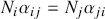 .
.
The meeting process in Rubinstein–Wolinsky can be interpreted in terms of spatial separation, even if they were not specific about it. A significant feature of their formulation is that the measure of type
 does not affect the probability
 meets
meets
 when
when
 and
and
 . Other papers proceed differently, and a common specification has the probability that
 meets
meets
 proportional to the fraction of type
 among the total population of participating agents in the market. This is sometimes called uniform random meetings, and implies the measure of
 in the market, for example, affects the probability
 meets
meets
 , which can be understood as a congestion effect that is assumed away in the original model.
Let
 be the probability of trade when
 meets
meets
 . With transferable utility, as described earlier,
 wants to trade with
 if and only if
 wants to trade with
 if and only if the joint surplus is positive, so we can use either
 or
or
 to indicate the probability they trade. Some of the
 s are trivial; for example,
 is automatic since when
 meets
meets
 with inventory
 , or
, or
 meets
meets
 with inventory
 , trade is impossible. The rate at which
 switches from
 to
to
 is
is
 , and the rate at which
 switches back is
 . In general, both are the product of chance (a meeting) and choice (a trade).
Let
 and
and
 be the value functions for
 and
and
 , and let
 or
or
 be the value functions for
 holding
 or
or
 unit of
 . As mentioned, here
 and
and
 leave after trading while
 stays. The surplus
 when
when
 trades with
 is:
is:
 (13)
(13)
 (14)
(14)
 (15)
(15)
where
 is assumed to produce upon meeting as in Rubinstein–Wolinsky.
For the terms of trade, with transferable utility, reasonable bargaining solutions all give similar results. Here we use generalized Nash bargaining: In each trade, the payment
 solves
 (16)
(16)
This yields:
 (17)
(17)
 (18)
(18)
 (19)
(19)
Thus, payment
 is a weighted average of the benefit to the agent receiving
 and the cost to the agent giving it up; for example, when
 gets
gets
 from
from
 the benefit to the former is
 while the cost for the latter is
 .
.
Also, with transferable utility, the best response conditions for whether
 and
and
 trade are given by:
 (20)
(20)
The original Rubinstein–Wolinsky setup has new
 and
and
 agents flowing into the market at an exogenous rate
 , making the stocks
 and
and
 endogenous. The stocks
 and
and
 are also endogenous, but of course we only need to keep track of
 since
since
 with
with
 fixed. Hence, the relevant laws of motion or the state of the system are
 (21)
(21)
 (22)
(22)
 (23)
(23)
where the
 s are derivatives with respect to time.
The value functions expressed in terms of
 satisfy
 (24)
(24)
 (25)
(25)
 (26)
(26)
 (27)
(27)
Consider (24). In words, it says the flow value
 is the rate
 at which
 meets
meets
 , times the probability
 they trade, times
 ’s surplus from that trade; plus the rate
 at which
 meets
meets
 with inventory, times the probability
 they trade, times
 ’s surplus from that trade; plus the pure rate of time change
 , which is
 in steady state but not in general. The other equations have similar interpretations.
With dynamic models we have to be a little more careful in defining things. An equilibrium here consists of paths for: the value functions
 , the terms of trade, which with
 indivisible are given by
 , the trading strategies
 , and the state variables
 , satisfying the dynamic programming equations, bargaining solutions, best response conditions, and laws of motion. Equilibrium must also satisfy an initial condition saying where the system starts in terms of N, plus the usual nonnegativity and boundedness conditions.Footnote 9 A stationary equilibrium is a special case where
 ,
,
 , and
, and
 are time-invariant functions of
 (they can depend on the state but not the date). A steady state is a solution to the equilibrium conditions other than the initial condition where endogenous variables are constant.
In Rubinstein–Wolinsky, as mentioned earlier, the arrival rate
 depends on
 and
and
 , the measures of
 and
and
 , but not on other
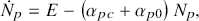
 s. This rules out third-party congestion in the meeting process, which is convenient, but the microfoundations may not be obvious. Figure 2 depicts a market structure consistent with their assumptions, featuring spatial separation, as in Gong et al. (Reference Gong, Qiao and Wright2024).
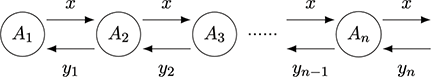
Market structure consistent with Rubinstein–Wolinsky (Reference Rubinstein and Wolinsky1987).
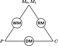
In Figure 2 different types are located at distinct locations represented by nodes on a triangle. Agents visit both of their nearby markets, represented by the edges, but not the third – it’s just too far. One can interpret this as saying there are three submarkets labeled as follows: a direct market (DM) with
 and
and
 ; a wholesale market (WM) with
 and
and
 ; and a retail market (RM) with
 and
and
 . This spatial separation is consistent with the Rubinstein–Wolinsky paper.
Now is a good time to discuss meeting technologies. Following textbook methods (e.g., Pissarides Reference Pissarides2000), consider a two-sided market with measures
 of buyers and
 of sellers. The number of meetings is assumed to be an increasing, concave function
 , implying arrival rates
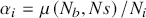 . A common assumption that we adopt is that
 displays constant returns to scale, which implies the arrival rates depend only on market tightness,
 . As mentioned earlier, and as Figure 2 shows, agents participate in both of their nearby markets but not the third.Footnote 10
This allows us to use a general two-sided meeting technology in each of the submarkets, which is convenient because it is not clear how to use a general meeting technology in a three-sided market (more on this in Sections 4, 6, 8, and 9). To proceed, let the DM, WM, and RM meetings technologies be
 , for
, for
 , where the
 s are constants describing search efficiency. Then, as in Rubinstein–Wolinsky, assume
 , but
, but
 can be different, and in particular
 is better than
 at meeting
 based on the fundamental technology when
 , although the equilibrium arrival rates depend on tightness.
Now, as in Rubinstein–Wolinsky, we focus on steady states that are symmetric in the sense that
 , which implies
 ,
,
 ,
,
 , and
, and
 . Also, as in their original model, we set
 . The goal is to determine the trading pattern given by the
 s. It is clear that
 and
and
 always trade (
 ). The more interesting questions are whether
 without inventory trade with
 (determined by
 ), and whether
 with inventory trade with
 (determined by
 ). Clearly, if
 then
then
 , since a buy-and-hold strategy for
 is not a good idea when
 . What remains to determine is whether
 and
and
 trade, as determined by
 .
.
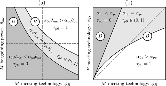
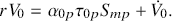
Although the Rubinstein–Wolinsky paper does not mention existence or uniqueness, from Gong et al. (Reference Gong, Qiao and Wright2024) we know that a symmetric steady state exists and is unique. This is illustrated in Figure 3. In the panel (a), on the vertical axis is
 ’s bargaining power, with the horizontal dashed line giving
 ’s bargaining power, so that above the line
 is better than
 at extracting surplus from
 . On the horizontal axis is
 ’s search efficiency, defined by
 in meeting technology,
 , while the vertical dashed line represents
 –so to the right of this line
 has a fundamental advantage in search. Panel (b) is similar but drawn in
 space.
Equilibrium set as a function of parameters.

Figure 3 shows there are regions of parameter space where
 and
and
 trade with probability
 , where they trade with probability
 , and where they trade with probability
 . In terms of the language introduced earlier, there are two possible outcomes: Regime D or B emerges when
 or
or
 . (Regimes
 and
and
 for now cannot emerge because
 is always in the market and happy to trade with
 for now – but see Sections 4 and 9) Related to Section 2, the result can be stated as follows:
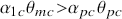 implies
 , so
, so
 and
and
 trade whenever they meet;
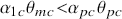 implies
 and
and
 never trade when they meet; and
 implies they sometimes trade when they meet.Footnote 11
This is a generalization of the Rubinstein–Wolinsky result, but as intuitive as it may be, the result is not totally satisfactory because it gives a relationship between the
 s and
s and
 s, both of which are equilibrium outcomes. Hence, it must be interpreted carefully. In particular, it is possible for
 to face a less efficient meeting technology, in the sense that
 is low, but due to endogenous tightness
 can still be high and hence
 still active. Indeed, as panel (a) of Figure 3 shows,
 is active when
 and
and
 have the same meeting technology and bargaining power, at the intersection of the two dashed lines, so by continuity
 is active with a moderate disadvantage in their meetings and bargaining. Similarly,
 might have a better
 and better
 than
than
 , yet
, yet
 .
.
So while the result is correct, it could easily be misinterpreted. However, the bigger point is that we now have a characterization of the
 s and
s and
 s in terms of parameters, as shown in Figure 3. In other words, there is a relationship between the
 s and
s and
 s, but it is not causal, since both are functions of other, more fundamental, factors.
Having made that point, beyond characterizing
 ’s activity, the theory has implications for how the terms of trade depend on fundamentals. One can check that both
 and
and
 decrease with an improvement in the meeting technology indexed by the
 s, which seems natural. However, the average
 paid by
 is nonmonotone because of composition effects – namely, faster search encourages participation by
 , and since
 charges more than
 , the average price paid by
 might increase. One can also check that price dispersion (as measured by, e.g., the coefficient of variation) can be nonmonotone.Footnote 12
We close this part of the discussion with an important modeling detail. The original Rubinstein–Wolinsky formulation has long-lived
 (they stay in the market forever) but short-lived
 and
and
 (they leave after one trade), with an exogenous inflow
 of the short-lived types. Consider an environment that is similar except
 and
and
 , as well as
 , stay forever, and in the interest of stationarity set
 . This makes the surpluses simpler because continuation values cancel with threat points,
 (28)
(28)
and the payments become
 (29)
(29)
 (30)
(30)
 (31)
(31)
Having all agents in the market forever has consequences. If, for example, type
 agents leave after trading, when they meet
 they may pass on trade to wait for a meeting with
 ; but if type
 stays after trading, at least with
 , we must have
 , allowing us to shift the focus elsewhere, like endogenous entry. Due to its relative tractability, several models presented herein have all agents in the market forever. A general point that one should always keep in mind is that modeling details like this can matter when exploring microfoundations.Footnote 13
4 Multiplicity and Dynamics
Some papers are concerned with whether we get uniqueness or multiplicity of steady state, and whether there are dynamic equilibria with fluctuations based solely on beliefs. This issue is obviously related to the venerable notion that intermediation, perhaps especially financial intermediation, might engender instability or volatility.Footnote 14 Now models based on Rubinstein–Wolinsky have dynamics: If the initial condition for
 is not at its steady state value, then the unique equilibrium is stationary and converges to steady state, so there is no instability or volatility. What happens if we deviate from the original formulation?
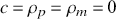
Nosal et al. (Reference Nosal, Wong and Wright2019) study a three-sided market where
 ,
,
 , and
, and
 interact via a uniform random meeting specification: conditional on
 meeting someone, the probability it is type
 is proportional to the fraction of type
 in the market. Normalizing
 , the rate at which type
 meets
meets
 is
is
 , where
 is a baseline arrival rate that is the same for all agents. Notice that rules out something that was the focus of the above analysis: It means
 and therefore
 cannot have an advantage over
 in finding type
 .Footnote 15
Even without an advantage in finding type
 ,
,
 can still be active for other reasons in Nosal et al. (Reference Nosal, Wong and Wright2019). In that paper, all agents stay in the market forever, which, as mentioned earlier, means that
 always trades with
 since there is no opportunity cost. This might suggest that
 agents are doing something socially valuable: When
 trades
 to
to
 they both become sellers, increasing the probability
 gets
gets
 . However, rather than having agents acting as
 to exploit this idea, it might be better to have them act as
 , because the best
 can do is to give
 to
to
 if
if
 has it in its inventory, while
 can give
 to
to
 whenever they meet. To pursue this, Nosal et al. (Reference Nosal, Wong and Wright2019) incorporate occupational choice: Anyone who is not type
 can choose to act as
 or
or
 , or to opt out of the market entirely.
That paper also plays up the distinction between markets for goods and markets for assets by identifying the former with
 and the latter with
 (although that is less relevant given an extension discussed later in this section). It is further assumed that
 produces a new unit of
 immediately after trading, before the next meeting, as opposed to producing in a meeting. Hence,
 as well as
 agents carry inventory. It is useful to have inventories depreciate – that is, vanish – at rate
 . Thus, a fundamental advantage for
 could be captured by
 or
or
 , although for simplicity we set
 .
.
Let us start with
 . Focusing for now on steady state, there are three possible outcomes: Regime
 , where the market shuts down; Regime D, where the market is open but no one chooses to act as
 , so there is only direct trade; and Regime B, where some agents choose to act as
 , so there is both direct and indirect trade. (Regime I is ruled out here because
 can only be active if some agents act as
 , since
 gets inventory from
 .) It can be shown that equilibrium exists uniquely: There is a unique steady state, and if we start away from steady state there is a unique transition path converging to it.
To give more detail, consider parameter space summarized by storage costs
 of
of
 and
and
 . It partitions into three regions: When
 is big for both
 , Regime N emerges, since storage costs are too high to make participation in the market worthwhile; when
 is below a threshold and
 above a (generally different) threshold, Regime D emerges; and when
 is somewhat higher and
 lower, Regime B emerges with both direct and indirect trade.
Now consider
 . This turns out to be rather different. First, Regime N cannot emerge for a production cost
 , or, more generally, for any
 that is not too big, since
 can always produce and hoard
 for its return
 . Therefore
 must produce, and when
 meets
meets
 they must trade, since
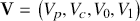
 can produce again. The possible outcomes are shown in panel (a) of Figure 4.Footnote 16
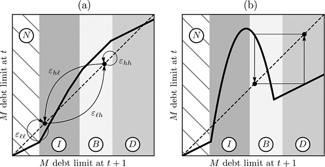
Multiplicity and dynamics.
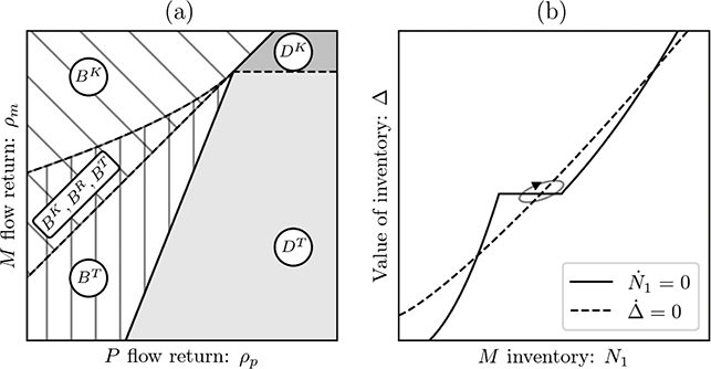
In the graph, there are steady states with
 , which is labeled as region
 or
or
 , where
 indicates direct trade and the superscript indicates what happens off the equilibrium path: If there were a type
 with
with
 , superscript
 says
says
 would trade it to
 , while superscript
 says
says
 would keep it (while these are the same on the equilibrium path, to show it is an equilibrium, as usual one has to know what happens off the equilibrium path).
Now consider steady states with
 . These are labeled
 ,
,
 , and
, and
 , where the
 indicates there is both direct and indirect trade, and the superscripts mean this:
 says
says
 trades
 to
to
 ;
;
 says
says
 keeps
keeps
 ; and
; and
 says
says
 randomizes. Naturally,
 obtains when
 is big and
 obtains when
 is small. What is interesting is that over some range, where
 is neither too big nor too small, there is multiplicity: two steady states coexist in pure strategies, one with
 and one with
 , and, as usual, when there are two pure strategy equilibria there is also a mixed strategy equilibrium with
 .
.
This multiplicity arises only for some parameters; for others there is a unique steady state with
 , which is
 if
if
 is small,
 if
if
 is big, and
 if
if
 is in between. But at least for some nondegenerate set of parameters there is multiplicity. Why? There are two necessary ingredients:
 , and
, and
 endogenous.
Here is the intuition. Suppose
 , which is like a buy-and-hold strategy by
 . That makes
 low (in fact, it is
 in steady state, although that changes if there is depreciation,
 ). When
 is low it is hard for
 to trade, so few agents choose to act as
 . That makes it hard for
 to get
 and hence makes
 reluctant to trade it away, so
 is a best response. Now, suppose
 . Then
 is high, making it easier for
 to trade, so more agents act as
 . Then it is easier for
 to get
 and so
 is a best response. For some parameters both outcomes are possible.
This discussion and Figure 4 concern steady states, but when there are multiple steady states there can also be multiple dynamic equilibria. These equilibria can display fluctuations even when fundamentals are constant: They are driven purely by beliefs, as self-fulfilling prophecies. Moreover, one can describe the outcomes in terms of market liquidity, which is greater with higher
 since that means more trade. Again, for this multiplicity to arise we need endogenous market composition, plus
 , since a buy-and-hold strategy is never a good idea when
 . This can be interpreted as saying that intermediated markets for assets, with
 , can be fragile or volatile, but not intermediated markets for goods, with
 .
.
Gu et al. (Reference Gu, Wang and Wright2026) change that result and interpretation. They show in a generalized environment that similar multiplicity and volatility can arise with
 . There are various differences between the papers. One is that instead of endogenizing market composition by having some agents choose to act as either
 or
or
 , Gu et al. (Reference Gu, Wang and Wright2026) fix the measure of each type but let type
 participate in the market only if they pay a cost
 . This is more standard than having agents choose to act as
 or
or
 , at least in the sense that it is similar to labor models following Pissarides (Reference Pissarides2000), where firms choose whether to enter, rather than having agents choose whether to be a worker or a firm (which is not to say that models of occupational choice are uninteresting).
A bigger difference is that Gu et al. (Reference Gu, Wang and Wright2026) have match-specific heterogeneity in buyers’ valuations: When a seller,
 or
or
 , meets
 the pair draw
 at random. This is interesting for its own sake and delivers nice results. First,
 ’s decision about trading with
 is characterized by a reservation value,
 , such that they trade when
 and not when
 , analogous to a reservation wage strategy in job search. It is immediate that
 since
since
 must be enough to cover
 ’s loss from giving up inventory. Moreover, this is nice because
 , and hence the probability of trade between
 and
and
 , varies smoothly with parameter changes and over time.
This introduces a new reason for
 and
and
 to not trade: The match-specific
 is too low. Of course,
 wants to trade even at low
 as long as
 is low, but
 means
means
 would have to be too low for
 to agree (the point is that trade requires mutual agreement). This effect is absent in Nosal et al. (Reference Nosal, Wong and Wright2019), where
 ’s alternative to trading with
 is to enjoy the flow
 , which is never a good alternative when
 . To be sure,
 discourages trade between
 and
and
 – the way unemployment insurance discourages acceptance in job search, say – but we do not need
 to get
 and
and
 to pass on trade.
The enhanced version of the story is this: Suppose
 agents adopt a high reservation value
 , which is not a buy-and-hold strategy, but a buy-and-hold-out (for a higher
 ) strategy. Then
 is high and
 low, making it hard for
 to trade so fewer
 agents enter, replacing the effect described earlier, which is that fewer agents choose to act as
 . Still, the outcome is similar: a low
 , making it hard for
 to get
 and rationalizing high
 . But if instead
 chooses low
 then
then
 will be low and
 high, making it easier for type
 to trade, so more
 enter the market, making it easier for
 to get inventory and rationalizing low
 .
.
Hence, in this environment, multiplicity due to beliefs does not require
 . Not only can there be multiple steady states here, there can be dynamic equilibria where trading strategies and market composition vary over time. Gu et al. (Reference Gu, Wang and Wright2026) use dynamical system theory to prove the existence of continuous time limit cycles – that is, equilibria where endogenous variables fluctuate in the long run – but since the methods are somewhat technical, using bifurcation theory, we do not go into detail (it is not that the math is especially difficult, with Azariadis Reference Azariadis1993, e.g., providing a textbook treatment geared to economists, but we think in this Element our time and space are better spent on other issues).
However, it is worth noting that the methods used by Gu et al. (Reference Gu, Wang and Wright2026) are difficult (if not impossible) to apply in Nosal et al. (Reference Nosal, Wong and Wright2019), where
 is degenerate, because with
 degenerate the dynamical system is not smooth: The probability that
 trades with
 jumps from
 to
to
 as the system goes from
 to
to
 . Hence, the existence of equilibrium cycles is not verified in that paper; in Gu et al. (Reference Gu, Wang and Wright2026) it is verified.
5 Private Information
Middlemen are often regarded as experts in assessing product quality, giving them a prominent role in markets for used cars, precious stones, antiques, art, etcetera. These markets are plagued by asymmetric information in the sense of Akerlof (Reference Akerlof1970). Do information frictions explain the emergence of middlemen? Do expert middlemen improve welfare? To address these questions, some papers incorporate information frictions into a middlemen framework.Footnote 17 In this section we introduce two of them.
Li (Reference Li1998) is similar in spirit to the Rubinstein–Wolinsky framework, while Biglaiser and Li (Reference Biglaiser and Li2018) model a one-shot game emphasizing adverse selection. In both cases, product quality is an endogenous decision of producers, and with information frictions their decision depends on others’ beliefs, which must be consistent with equilibrium. This self-fulfilling feature naturally supports multiple equilibria. Li (Reference Li1998) highlights this kind of multiplicity, while Biglaiser and Li (Reference Biglaiser and Li2018) focus on cases with a unique equilibrium.
Li’s (Reference Li1998) model is related to Williamson and Wright (Reference Williamson and Wright1994), which is simplistic in the sense that all goods are indivisible, but such models can still make interesting points. Time is continuous and there are random bilateral meetings. A continuum of homogenous agents produce, trade, and consume a good which can be of low or high quality,
 . The
. The
 good costs
 and yields
 utility from consumption; the
 good costs
 and yields utility
 . All agents have the option of becoming
 by paying a fixed cost
 that can be interpreted as acquiring a quality-testing technology, in addition to
 , the cost to produce an
 good. Let
 denote traders that do not choose to act as middleman and normalize
 .
.
Assume
 can verify whether quality is
 or
or
 with probability
 , while
 can always verify quality. Agents first choose occupation,
 , then
 agents choose
 . When agents meet they decide whether to trade after potentially verifying quality, and note that the occupation,
 or
or
 , is recognizable upon meeting. When two
 s trade, they simply swap goods. When
 trades with
 , assume that
 makes a take-it-or-leave-it offer:
 gives up
 units of the good for A’s whole unit, and
 consumes what they receive, while
 consumes
 and seeks to retrade the good.Footnote 18 Upon consuming once,
 starts over by again choosing
 , as does
 after completing one round of intermediation (as discussed earlier in the context of other models, here everyone is in the market forever).
Note that
 may have an incentive to accept
 goods, as they get to consume
 units of
 goods from each round of intermediation. Thus, there are in principle four types,
 , capturing occupation and inventory, and
 indicates the corresponding payoffs. In equilibrium, the best response for occupational choice satisfies
 (32)
(32)
The participation condition for
 with
with
 good is
 . The production decision satisfies
 (33)
(33)
Two other best responses are whether
 accepts unknown quality and whether
 accepts
 . If
. If
 never accepts
 , they are honest; if
 always accepts
 , they are dishonest; and they may mix in between. These decisions depend on others’ beliefs and strategies. In equilibrium, individual strategies must be consistent with beliefs.
This model captures the following aspects of middlemen: they emerge endogenously; they have an informational advantage over others; and they may or may not be trustworthy. It is shown that when
 and
and
 are low, there are active
 and they always trade high-quality goods. This means
 choose to be honest because there are enough informed agents playing a disciplinary role. For moderately high
 ,
,
 can mix, trading both
 and
and
 goods. When
 is even higher, there are multiple equilibria, with
 and
and
 as well as with
 and
and
 . See Figure 5.
Equilibrium set with (panel (b)) and without (panel (a)) middlemen.

In this framework,
 improves efficiency by increasing
 ’s incentives to produce high quality, and consequently improving
 ’s acceptance of high quality. However,
 spends more time trading rather than producing, so higher
 reduces total output. These two forces determine
 ’s impact on welfare. Though across equilibria with
 and
and
 ,
,
 can be welfare improving, the occupational choice is typically suboptimal. Specifically, Li (Reference Li1998) shows
 is too big.
The approach in Biglaiser and Li (Reference Biglaiser and Li2018) is different: Agents have fixed types –
 ,
,
 and
and
 – and the paper compares equilibrium outcomes with and without
 . In their baseline model,
 pays
pays
 for effort
 that affects the probability of producing
 goods. Again,
 good yields
 for
for
 and
and
 good yields
 . Here
 do not get utility from consuming the good, but profit from payments in the form of transferable utility. Also,
 faces an entry cost
 to be active.
In terms of quality verification,
 ’s technology is no longer perfect: They receive a noisy signal that is correct with probability
 , which still gives
 an advantage over other agents who receive an inferior signal, which is correct with probability
 . The imperfect signal induces a misidentification effect, where
 with
with
 generates a positive signal with
 . The opportunity to fool
 gives
gives
 an additional avenue besides selling directly to buyers
 goods pretending to be
 goods, which always reduces
 ’s incentive to invest in quality. This means the presence of
 can reduce welfare via this effect.
Meanwhile, instead of meeting each other randomly, the agents here meet sequentially. Consider
 and
and
 . After producing a unit,
 first meets
 , who receives a private signal and makes a take-it-or-leave-it offer. If
 and
and
 trade,
 brings the good to
 ; if
; if
 and
and
 do not trade,
 seeks to trade with
 . Then both
 s receive a public signal and bid independently and simultaneously, with the winner getting the good. This sequential structure induces adverse selection: As
 is more likely to trade with
 ,
,
 rationally adjust their belief about
 ’s quality in direct trades. This again lowers the incentive for
 to invest in quality.
Biglaiser and Li (Reference Biglaiser and Li2018) show uniqueness by focusing on cases where the cost
 of becoming type
 is moderate, and the marginal cost
 of quality is either high or low (but not intermediate, since intermediate marginal cost might induce multiplicity). In this case, in equilibrium, better information does not necessarily improve welfare. In particular, as
 , it turns out that
 always chooses the minimum effort. Note that whenever
 encounters
 , the latter has already been rejected by
 with a perfect signal. Therefore,
 agents believe such a
 always carries
 goods and hence refuse to trade. It follows that when
 trades with
 ,
,
 loses the outside option of trading with
 . Given that
 makes a take-it-or-leave offer,
 faces a severe holdup problem and thus never exerts effort.
Not only can better technology reduce welfare, greater competition can as well. Intuitively, when many
 obtain private signals and compete, a
 who shows up in direct trade must be holding
 goods, which again eliminates
 ’s outside option of trading with
 and induces minimum effort. This result follows from the sequential structure of the model. Spulber (Reference Spulber2002) also studies intermediated trade with asymmetric information, but in his setup
 ,
,
 , and
, and
 move simultaneously, and then competition among
 agents improves welfare.
From these papers one sees that information and intermediation can interact in complex ways. While
 may be active due to information frictions, the welfare effects are ambiguous. A better verification technology undoubtedly reduces informational asymmetries, but the resulting impact on occupational choice and adverse selection can offset or even reverse the benefits of better information. Such results are important and suggest that even more work should be done on intermediation and information.
6 Intermediation Chains and Bubbles
Wright and Wong (Reference Wright and Wong2014) study middlemen chains, asking how they form, how many intermediaries might be in a chain, and how bargaining at one link in the chain depends on bargaining at future links. This is relevant since in reality there are often multiple middlemen engaged in getting goods (or inputs or assets) from originators to end users: for example, from farmer to broker to distributor to retailer to consumer.
Internet trade provides a prominent example of these structures. Many advertised wholesalers are actually intermediaries operating within a chain of middlemen. This occurs when a business purchases products from a wholesale company that has itself sourced them from another wholesaler, potentially continuing through multiple layers.
Another example concerns real estate flipping, where a property is purchased and quickly resold for profit. Under a multiple investor flip, one investor acquires a property below market value and sells it to a second investor, who then sells it to the final consumer at a price closer to market value. These profits are typically generated by buying low and selling high in a rising market or by renovating a property before resale.
Here agents acting as middlemen do not have an advantage in information or technology, they are simply a necessary part of the process of getting goods from suppliers to end users. An interpretation (suggested by Dale Mortensen; see fn. 18) is that to move goods from location
 to
to
 , they must travel through
 ,
,
 and those with property rights to the intermediate locations all want a cut of the profits.Footnote 19 Figure 6 depicts the market structure – a simple network – and hence the potential transactions.
Market structure consistent with Wright–Wong (Reference Wright and Wong2014).

The formalization has time continuous and potentially unbounded, with a set of agents
 , where
 may or may not be finite. These agents are spatially separated:
 can trade with
 and
and
 but no one else. Hence, trade between
 and
and
 must go through
 , and there is no scope for cutting out the middleman.Footnote 20 The friction is that it takes time for
 to meet
 , with
 the Poisson arrival rate. As noted earlier, there is an indivisible object
 and a divisible object
 , and
, and
 is endowed with
 . If
. If
 acquires
 from
from
 , then
 can consume it for payoff
 or try to trade it to
 for
for
 , which in general yields payoff
 . As discussed earlier,
 corresponds to transferable utility, but it is also interesting to consider
 later in this section.
The Wright and Wong (Reference Wright and Wong2014) model uses a particular bargaining protocol that is nice but not crucial for the results – all that really matters is that agents trade when there are gains from trade. In any case, if
 with
with
 does not consume
 , but tries to trade it, the flow payoff is
 , or
, or
 (34)
(34)
where
 is an
is an
 -specific search or storage cost. Then
 wants to trade when
 . If
. If
 equilibrium is found by starting at the last link in the chain, where
 with
with
 meets
meets
 , since
 must consume
 – there is no one left with whom to trade. Hence,
 implies
 consumes
 and
and
 implies
 consumes it after giving
 to
to
 . Assuming
 , we get
 (35)
(35)
after inserting
 , where
 is bargaining power. Hence, search by
 requires
 , or
, or
 (36)
(36)
If
 there is generically a unique equilibrium that, depending on parameters, can involve anything from
 consuming
 to the opposite extreme, where
 consumes it. In general, there is maximal length of the intermediation chain. If the environment is stationary (parameters are the same for all
 ) then one can check that as times moves forward, so that
 is getting closer to its end user,
 increases with every trade, and, in fact, it increases at an increasing rate.Footnote 21
To expand on the results, let
 be the random date when
 trades
 to
to
 . Since the arrival times are Poisson, the interarrival times
 are distributed exponentially (see any source on stochastic processes, e.g., Çinlar (Reference Çinlar1975)). This means there is a high probability of short interarrival times and a low probability of long interarrival times, and so typical realizations have trades clustered, with many exchanges occurring in relatively rapid succession, separated by long periods of inactivity. This might look like bubbles in the market, with long lulls interspersed by trading frenzies where
 accelerates over time. But
 accelerates only because
 is getting closer and closer to the end user, and Poisson arrivals are memoryless, so there are no bubbles, or frenzies and lulls, in any meaningful economic sense.Footnote 22
However, there can be genuine bubbles when
 , related to standard results in monetary theory. To pursue this, first note that money and middlemen papers would take diametric positions on this: The former would say
 is a good and
 is money; the latter would say the opposite. Which makes more sense? Well,
 being divisible is a point in favor of middlemen papers, since divisibility is a property commonly associated with money, but we think that should not be given much weight compared to the functional definition of money: that it is a store of value and medium of exchange.
Clearly, it is
 and not
 that is a store of value:
 is a durable object that when acquired lets
 enjoy a payoff at some future date. And it is a medium of exchange according to standard usage – an object accepted in trade not to be consumed or used in production but to be traded again later. Indeed,
 solves the standard double-coincidence problem that makes money useful: When
 wants
wants
 from
from
 , the only way to pay is by transferring
 . On these grounds,
 looks like money.
Does this matter for anything? Maybe. It determines who should be called buyers and sellers and what defines the price. In nonmonetary exchange –
 gives
gives
 apples for bananas – it is not meaningful to call either a buyer or a seller. But if
 gives
gives
 apples in exchange for cash then
 is the seller and
 is the buyer. While one can use words as one likes, would anyone suggest, for example, reversing the worker and firm labels in standard labor-market models? One could prove similar results, but it matters for substantive questions – for example, should we tax/subsidize workers or firms? It similarly makes a difference for who we call buyers and sellers – for example, should we tax/subsidize shoppers or retailers? Moreover, normalizing the size of
 to
to
 , if
, if
 is money and
 is a good the price is
 , while if
 is a good and
 is money the price is
 . This matters for the foregoing discussion of
 accelerating – is that a hyper-inflation or a hyper-deflation?
So, one can think of
 as a good potentially passing from originator to end user via a chain of intermediaries trading at each link for
 ; or, one can think of
 as a medium of exchange allowing agents to acquire
 . This is one reason to allow nonlinear
 . There is another reason. Suppose
 . As is understood in monetary economics, there can be bubbles in the sense that no one ever consumes
 , agents just keep trading it, like a vintage wine market where people trade and retrade bottles no one will ever drink, or a POW camp where prisoners trade cigarettes no one will ever smoke. Moreover,
 can be above the fundamental value of
 , given by the utility of consuming it. There exist such bubbly equilibria here if
 , but not if
 is linear (see Wright and Wong Reference Wright and Wong2014 for details).
We pursue something similar but more sophisticated: the application in Awaya et al. (Reference Awaya, Iwasaki and Watanabe2022). That paper constructs a finite-period model of bubbles where the indivisible good is considered an asset. In contrast to the specification given earlier, where bubbles can occur only if there are an infinite number of middlemen and periods, Awaya et al. demonstrate that bubbles can occur with a finite number of traders and periods. When the horizon is finite, a standard backward induction argument implies that, if everything is common knowledge, bubbles never occur. Awaya et al. relax the assumption of common knowledge and consider higher-order uncertainty. This means that even if every agent knows the fundamental value of the asset is 0, agents may not know whether other agents know it.
The information structure is key here. Following the definition of strong bubbles in Allen et al. (Reference Allen, Morris and Postlewaite1993), a bubble occurs if all agents know the indivisible asset is worthless but it is traded for a positive amount of the divisible good. There are two necessary ingredients for this. First, there must be at least one agent who may not know the consumption value of the asset for
 – otherwise, the value is commonly known and the asset can never be overpriced. Second, there must be some situations where the consumption value of the asset for
 is zero and all agents know it.
To capture this, assume that all parameters describing utilities, costs, etcetera, are common knowledge, except for the consumption value of the asset for
 . Awaya et al. assume that, prior to trade, all agents except
 observe the consumption value of the asset for
 . Hence, the initial owner and the middlemen are experts who always know the value of the asset, while the final user is not an expert and may not know.Footnote 23
If the consumption value of the asset for the end user
 is
is
 , then
 receives a signal with some probability; otherwise,
 does not receive a signal. Thus, if
 receives a signal,
 is sure that the consumption value of the asset for
 is
is
 , and every other agent also knows the asset is worthless. Moreover, if
 receives a signal,
 (nonstrategically) sends a signal to
 . The signal reaches
 with some probability but can also be lost. Thus, if
 receives a signal,
 is sure that
 knows that the consumption value for
 is
is
 . Similarly, if
 receives a signal from
 , then
 (nonstrategically) sends a signal to
 . Again, the signal reaches
 with some probability but could be lost. This process continues until a signal is lost between some two agents or the initial owner
 receives a signal. In words, the signal (rumor) that
 knows that the asset is worthless spreads from
 to
to
 , but it is subject to loss between any two agents.
With this information structure, bubbles occur at some states. Consider the state where the consumption value of the asset for the final user
 is
is
 and the signal between
 and
and
 is lost for some
 . In this state,
 receive signals, while the rest do not. Given this realization, since
 receives a signal, every agent knows that the asset is worthless. Yet the asset is exchanged for
 periods, until it reaches
 . This is a bubble. If it were common knowledge that the consumption value of the asset for
 is
is
 , the asset would not trade. Therefore, higher-order uncertainty is necessary for bubbles. At period
 , agent
 refuses to trade with
 and the bubble bursts. This is because
 knows that
 knows that
 that
that
 knows that the consumption value of the asset for
 is
is
 , and hence,
 knows that
 cannot sell the asset to
 .
.
Middlemen here are necessary for bubbles. Without them, there is just the initial owner and the final user, and if both know the asset is worthless they do not trade and bubbles do not occur. In this sense, middlemen are a source of instability. Awaya et al. (Reference Awaya, Iwasaki and Watanabe2022) also characterize prices during bubbles, interpreting the asset price as
 . This price is not only increasing, it is accelerating during bubbles, because middlemen must be compensated for the risk that they may not be able to retrade the asset. That is, this price accelerates because the probability that a middleman can sell it decreases over time, so those who trade in later periods are exposed to more risk, and the price compensates for that.
In a follow-up paper, Awaya et al. (2025)Footnote 24 integrate their analysis of bubbles into the monetary model of Lagos and Wright (Reference Lagos and Wright2005) to study, among other things, how a monetary policy affects the results. They show that the existence of bubbles depends on the degree of money injection. This is frontier research and a nice example of what one can do in models that incorporate both money and middlemen, which is discussed further in Section 9. Before going there, however, it is a good time to discuss work that amends some of the basic assumptions in the benchmark model.
7 Inventories and Directed Search
The models presented so far focus on
 . In reality, inventory and variety are common attributes of retailers and dealers. A few papers go beyond this restriction. Nosal et al. (Reference Nosal, Wong and Wright2019) have an extension of their baseline model with
 that they study using numerical methods, but we will not go into that. Instead, we highlight two other strands in the literature: One examines the distribution of middlemen’s inventory size and composition with random search; the other focuses on the impact of inventory with directed search. Note that the inventories in this section take discrete values, which has implications for matching.Footnote 25
Shevchenko (Reference Shevchenko2004) relaxes the assumption of fixed inventory size in an environment with a continuum of agents and
 different goods.Footnote 26 Agents have heterogeneous tastes for goods: agent
 produces good
 at
at
 cost (for simplicity) and desires another good drawn at random. Since they both consume and produce, we do not label them as
 or
or
 and simply call these agents type
 . They can trade bilaterally when they meet if there is a double coincidence of wants, where each one likes the good the other produces. In addition,
 can meet
 , a middleman. Type
 have a cost to enter the market, so the measure
 is endogenous. Also, each
 maintains a capacity
 – the number of shelves – by paying a flow cost
 , allowing them to store
 goods. The cost of getting the initial inventory
 is part of
 ’s cost of entering the market.
In steady state, if
 and
and
 meet and
 has in stock the variety that
 wants, trade occurs. The way it works is this:
 gives the good that
 produces to
 , who puts it on the shelf that opens up by taking the good
 likes off the shelf; then
 consumes some fraction
 of the good while
 consumes the rest. This can be interpreted as
 having a technology to transform any good into something
 likes, with the cost of the technology being part of their operating cost
 .
.
Shevchenko (Reference Shevchenko2004) demonstrates the existence of a unique and stable steady-state distribution of inventories – all
 have the same shelf size
 and the variety distribution is uniform across
 . He shows that size
 increases with
 ’s bargaining power and arrival rate. In terms of welfare, on the intensive margin, middlemen always understock relative to the optimum:
 is too small. This occurs because
 chooses
 upon entering the market, and the cost
 is sunk when
 shows up. The resulting hold-up problem makes
 too low. On the extensive margin, the number of
 can be too big or too small, depending on parameter values.
In the aforementioned formulation
 ’s choice of
 does not affect their arrival rate: meetings are purely random. Now consider a situation where buyers can choose where to search – which shop to visit – based on the size of their inventory. This suggests a directed search approach, where consumers select sellers based on their posted prices plus their inventory, which is assumed to be observable. Directed search provides an interesting and (in some contexts) realistic way to endogenize trading patterns.
Watanabe (Reference Watanabe2010) describes a static game in which middlemen can have multiple units in inventory and can transact with multiple agents simultaneously. Because they can serve multiple agents, the matching process is many-to-one. Watanabe adopts a coordination game framework, as in Burdett et al. (Reference Burdett, Shi and Wright2001). If a seller has
 units of the good, and more than
 buyers show up, only
 of them get the good. This endogenously generates the number of trades as an urn-ball technology.
With a continuum of agents, the equilibrium can be characterized by best responses and the market utility condition that all sellers must provide the same expected payoff to buyers. Intuitively, if one seller offers a higher expected payoff, buyers will have an incentive to go to that seller, pushing the equilibrium toward payoff equivalence. The implication is that, by holding more inventory, middlemen reduce their probability of stockouts, and hence can charge more than producers who can serve at most one customer. The ability to have multiple units in inventory thus gives
 a role.
Watanabe establishes an equilibrium in which a unit mass of agents choose to be acting as type
 or
or
 , and the latter obtain inventories from
 in a competitive wholesale market. With a fixed cost
 to become a middleman,
 is determined by
 . Occupational diversity here requires indifference if agents are ex ante homogenous. If agents are heterogenous, occupational choice typically leads to cutoff rules, similar to, for example, the models in Masters (Reference Masters2007, Reference Masters2008).
When
 , there is a unique equilibrium with intermediated trade,
 . In contrast, when
 , an equilibrium with
 requires a low
 , and multiple equilibria can arise: one with high
 , high
 , and small
 , and another with low
 , low
, low
 , and large
 . Multiplicity here stems from the nonmonotone nature of the spread
 in capacity
 . This is supported by empirical evidence (e.g., Dana and Spier Reference Dana and Spier2001 on video rentals; Li et al. Reference Li, Murry, Tian and Zhou2024 on used cars; Aguirregabiria Reference Aguirregabiria1999 on supermarkets; Leslie Reference Leslie2004 on theater tickets). Watanabe (Reference Watanabe2010) also shows that the equilibrium with many small middlemen is stable but inefficient, whereas the one with fewer large middlemen is unstable but more efficient.
Recall that in Shevchenko (Reference Shevchenko2004) inventory and variety play a role, whereas Watanabe (Reference Watanabe2010, Reference Watanabe2020) considers inventory but not variety. Moraga-Gonzalez and Watanabe (Reference Moraga-Gonzalez and Watanabe2023) incorporate variety into a directed search environment while maintaining capacity
 . Specifically, goods are differentiated, and consumers learn their match-specific value upon visiting a seller. The matching function is accordingly generalized: When
 , it follows an urn-ball specification; as
 , it converges to a weighted urn-ball technology (see, e.g., Lester et al. Reference Lester, Visschers and Wolthoff2017), with the weights reflecting match-specific values. The equilibrium price is inefficiently high, except in the limit as
 . In addition to variety, Rhodes et al. (Reference Rhodes, Watanabe and Zhou2021) incorporate cross-product externalities and show how variety alone can justify the emergence of middlemen.
In sum, inventory size and variety are potential sources of
 ’s advantage, distinct from capabilities like bargaining power or search efficiency. When their advantage comes from bargaining or search, one can determine whether replacing
 with
with
 generates surplus. Inventory and variety, by contrast, create a middlemen advantage through the matching process and the implied terms of trade.
In addition to providing some microfoundations for
 ’s higher meeting probabilities, directed search provides an alternative way to endogenize prices, capturing the role of middlemen in posting publicly observable terms of trade (Spulber Reference Spulber1996b). This insight is sharpened by Watanabe (Reference Watanabe2018), who contrasts random search and bargaining, on the one hand, with directed search and posting, on the other hand. While the existing models and results are nice, this is a branch of the literature that merits even more research.Footnote 27
8 Intermediation in Finance
Many financial markets are highly intermediated. In OTC asset markets, investors who want to trade must search for counterparties and negotiate the terms of trade. Duffie et al. (Reference Duffie, Garleanu and Pederson2005) provide a model of OTC trade that sheds light on many issues, including standard measures of liquidity, like bid-ask spreads, execution delays, and trading volume.Footnote 28 These models share some features with those discussed elsewhere in this Element, but differ in other aspects.
In the typical finance paper, there are no producers or consumers – the object being traded, denoted
 as usual, is an indivisible asset in fixed supply
 . A fixed set of agents, labeled
 , get a flow return
 from holding the asset, and as in many other models individual inventories are restricted to
 . Assuming
 is scarce (i.e., there are fewer assets than agents), gains from trade are generated by random idiosyncratic valuations. Namely, these agents have a state variable given by
 or
or
 , and according to Poison process this valuation switches over time from
 to
to
 at rate
 , independent of
 .
.
So at any point in time there can be some agents with low valuation
 and
and
 , as well as some with high valuation
 and
and
 . If they meet there are gains from trade, with payments made in transferable utility, which again we interpret in terms of another good anyone can produce with constant marginal cost and anyone can consume with constant marginal utility. Let
 be
be
 ’s value function with asset position
 and valuation
 and let
 . It is immediate that
 trades with another
 when one has
 while the other has
 .
.
In addition to type
 agents, there are type
 agents, often called dealers in these papers, who can buy and sell assets. For simplicity, suppose they get
 return from holding the asset, but, in fact, usually in these models
 never holds inventory, with exceptions like Weill (Reference Weill2007, Reference Weill2008) or Gavazza (Reference Gavazza2011). The reason is that they can always access a competitive, frictionless interdealer market (with type
 excluded from this market). Therefore,
 in contact with
 that has
 and
and
 can in principle buy the asset from
 and sell it on the interdealer market, while
 in contact with
 that has
 and
and
 can sell the asset to
 while acquiring it on the interdealer market.Footnote 29
In the interdealer market, it is not generally the case that the number of type
 trying to buy the indivisible asset from
 equals the number of type
 trying to sell it to
 . Hence, the interdealer price makes
 and
and
 on the long side of the market indifferent to trade, with the number of such trades set to get what is needed on the short side: If
 , then
 meet more potential buyers than sellers and the interdealer price is
 ; and if
 , then
 .
.
As usual, what is called the bid price
 and ask price
 are determined through bargaining, with
 being
being
 ’s share of the surplus, which is
 or
or
 when selling or buying. It follows that
 (37)
(37)
 (38)
(38)
The bid-ask spread
 is a common indicator of asset market friction. The price
 between two agents of type
 is also determined by bargaining, with
 being the surplus share of the one bringing the asset to the meeting.
Normalize the measure of
 with
with
 , where
 is the proportion of
 with position
 and valuation
 . Denote by
 and
and
 the Poisson rates of
 meeting
 and
and
 meeting
 . The dynamic programming equations are
 (39)
(39)
 (40)
(40)
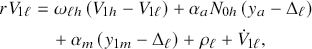 (41)
(41)
 (42)
(42)
In words, (41) says the flow value
 is: the rate
 at which
 switches from
 to
to
 times the change
 ; plus the rate
 at which
 meets another
 , times the probability the other one wants to trade
 , times
 ’s surplus; plus the rate
 at which
 meets
meets
 times the surplus for
 trading with
 ; plus the pure rate of change over time
 . The others are similar.
The laws of motion satisfy
 (43)
(43)
 (44)
(44)
 (45)
(45)
 (46)
(46)
An equilibrium is a list
 satisfying the usual conditions, and it exists uniquely (Trejos and Wright Reference Trejos and Wright2016). From this, the terms of trade, the bid-ask spread, and other endogenous variables are easily recovered.
This stylized structure, with a core of dealers and a periphery of others that may trade directly or with dealers, is a reasonable representation of many OTC markets. The proportion of intermediated trade is
 . Hence, the majority of exchanges can be direct, or intermediated, depending on parameters. A simple case where
 is nice since it makes the
 s and
s and
 s independent of
 . That makes it easy to see that spreads are decreasing in
 and increasing in
 . Also, as
 ,
,
 ,
,
 , and
, and
 all go to the same limit, which is
 if
if
 and
and
 if
if
 .
.
There are also implications for trade volume, often associated with liquidity, but these are sensitive to
 . That inventory restriction is relaxed in Lagos and Rocheteau (Reference Lagos and Rocheteau2009) and Üslü (Reference Üslü2019), who have continuous asset positions. Another extension is Farboodi et al. (Reference Farboodi, Jarosch, Menzio and Wiriadinata2025), who stick to
 , but their environment has no type
 . Instead, intermediation emerges since agents differ in bargaining power.Footnote 30 Given transitory valuations as in Duffie et al. (Reference Duffie, Garleanu and Pederson2005), agents with stronger bargaining skills act as middlemen, buying assets from those with low bargaining power and low valuation, and selling to those with high valuation and low bargaining power.
This brings up a question: just because some agents buy now and sell later, are they middleman? If you bought a house in year the 2000 and sold it in 2025, perhaps because you were moving out of town, it does not seem reasonable to say that you were engaged in real estate intermediation (there are agents that are so engaged, and they are called real estate flippers). Type
 in many of the models presented here are dedicated middlemen; agents in other models may trade a lot–say, because they have frequent preference shocks–but we are not convinced that they should be called intermediaries.
It may sound reasonable to think that a survey of middlemen in search equilibrium ought to provide a precise definition of a middleman, but doing so is not straightforward. The standard dictionary definition – “a person who buys goods from producers and sells them to retailers or consumers” – rings true, and is fully consistent with many of the models. Yet it is not immune to the housing example: you could have bought the property from a builder and sold it to someone who wants to live in it, or maybe flip it, and that does not make you a middleman. Perhaps a more holistic approach is better.
This ambiguity is not unique to the finance literature, as it applies, to a greater or lesser extent, in any of the models summarized here–although one could try to argue that it is more of an issue in settings where there is no producer or consumer of the object being traded. In any event, there are many papers building on the OTC framework, with or without dealers. Rather than discuss them in detail here, we refer readers to the recent and comprehensive book by Hugonnier et al. (Reference Hugonnier, Lester and Weill2025).
However, we can discuss a connection between the finance literature and monetary economics. The OTC model with
 (no middlemen) is best for this comparison, even if in this Element that is not the most interesting case. In finance models following Duffie et al. (Reference Duffie, Garleanu and Pederson2005), gains from trade arise from heterogeneous valuations for
 , with
 serving as a payment instrument. Monetary models following Shi (Reference Shi1995) or Trejos and Wright (Reference Trejos and Wright1995) have many of the same ingredients, but there are gains from trade in
 and the asset
 is used as a payment instrument. These gains from trade arise when
 for some
 , which has quite a different implication than the transferable utility assumption with
 . Trejos and Wright (Reference Trejos and Wright2016) further explore the connection between the approaches, integrate them, and highlight some key results.Footnote 31 While this is not directly related to intermediation, it is good to understand the similarities and differences in the finance and monetary papers, especially since both purport to be about liquidity.
9 Money, Credit, and Middlemen
In general, money and middlemen provide a similar service: the institution of intermediated exchange and the institution of monetary exchange are both ways of ameliorating trading frictions. There are a few, but not very many, papers with both middlemen and money, even if it is recognized that there are connections between intermediation and payment economics.Footnote 32 Li (Reference Li1999) is an early paper in this vein, showing how qualitative uncertainty over goods can give rise to both middlemen and fiat currency. In a pure barter economy, agents cannot verify the quality of goods they are offered, so some optimally invest in a costly inspection technology and thus become middlemen. These expert intermediaries can mitigate adverse-selection frictions while currency helps with double-coincidence frictions. This is a nice point, although the model in Li (Reference Li1999) is simple, assuming indivisible goods and assets.
Urias (Reference Urias2018) has monetary trade in a model of middlemen that gets at some key ideas, but it is also somewhat restrictive in that producers are not allowed to trade directly with consumers. Gong (Reference Gong2018) uses a similar environment, but focuses on credit rather than money and lets producers try to trade directly with consumers, making equilibrium exchange pattern endogenous – it can have only direct trade in
 from
from
 to
to
 , only indirect trade from
 to
to
 to
to
 , or both, depending in a precise way on parameters. These papers build on the framework of Lagos and Wright (Reference Lagos and Wright2005), which features sequential trade in different markets.
We can describe this in more detail following the presentation in Gong and Wright (Reference Gong, Qiao and Wright2024). First, the model has something not in most middleman papers: To capture the intensive margin,
 is divisible, which can be interpreted in terms of either quantity or quality. (To be precise, the extensive margin refers to the number of trades and the intensive margin refers to the size of trades.) While that is interesting in its own right, the bigger distinction from many previous models is the market structure, shown in Figure 7, interpretable as sequential trade in discrete time. First there is a wholesale market (WM) where
 and
and
 can, but
 cannot, participate; then there is a retail market (RM) where
 can trade with sellers, where these RM sellers can be either
 that acquired
 from
from
 in WM, or
 that did not trade with
 in WM and try for direct trade in RM. Sellers, both
 and
and
 , may or may not try to trade in RM because there is an entry cost
 .
.
Market structure consistent with Gong (Reference Gong2018).
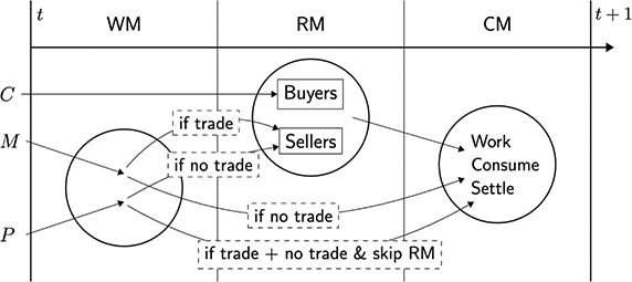
After WM and RM, there convenes a frictionless centralized market (CM) where all agents work, consume, and adjust their assets or debt positions. In monetary versions, like Urias (Reference Urias2018), one’s asset position can include currency; in credit versions, one’s debt position can include accounts payable from purchases made in the previous WM or RM, plus accounts receivable from sales in the previous WM or RM. A common device in Lagos–Wright applications is to assume quasi-linear utility in consumption of a numeraire CM good (in fact, quasi-linearity can be relaxed, as in Wong Reference Wong2016). Assuming interior solutions for CM optimization, this implies history independence: In money models, all agents of the same type leave the CM with the same cash; in credit models, all agents settle debts in the CM, and, moreover, one-period debt is without loss of generality.
This sequential structure replaces the three-sided market, where
 ,
,
 , and
, and
 all participate, with two two-sided markets, one with
 and
and
 , and one with buyers and sellers, where buyers are type
 while sellers can be either
 or
or
 , who may differ in various ways but can be treated symmetrically with respect to the meeting technology, which allows us to specify that technology rather generally. It may be useful to compare the market structure here with that in Figure 2, where one might say the former concerns temporal separation and the latter spatial separation.
This structure is nice because history independence makes it about as tractable as a typical three-period model, and so without too much additional work we can consider infinite-horizon models. The infinite horizon is critical under standard assumptions if, e.g., one wants to support exchange using fiat currency or support unsecured credit.
Gong and Wright (Reference Gong and Wright2024) show that with exogenous debt limits, equilibrium exists and is unique. Also, they show that one of four trading patterns, called regimes, will emerge: no trade (Regime N); direct trade only (Regime D); indirect trade only (Regime I); or both direct and indirect trade (Regime B). Panel (a) of Figure 8 illustrates how the outcome depends on search efficiency. When search efficiency is low, the market shuts down; when it is moderately higher, the exchange pattern depends on the relative advantage of
 and
and
 in search efficiency and bargaining power. If
 has no advantage over
 , there is no gain from WM trade and we get Regime D. If
 has an advantage, WM trade occurs if
 meets
meets
 , and
, and
 that fails to trade in WM may either enter or skip RM depending on search efficiency, corresponding to Regimes B and I.Footnote 33
Equilibrium set in search efficiency (panel (a)) and credit limit (panel (b)).
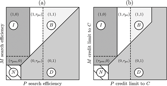
With divisible goods, bargaining power shapes not only the division of surplus but also its size. Specifically, greater seller bargaining power raises buyer payments but also increases the equilibrium quantity/quality of
 . As a result, higher bargaining power for
 and
and
 can improve
 ’s payoff – a novel insight in the sense that it cannot happen with indivisible goods. But the bigger contribution may be to introduce a new dimension along which middlemen may have advantages: They are better at using credit, by more reliably promising future payment or enforcing payment by others. This can be captured with exogenous debt limits by saying the limit when
 buys
buys
 from
from
 – call it
 – is big or the limit when
 sells to
 is bigger than when
 sells to
 – say
– say
 .Footnote 34 One can also consider credit more along the lines of Kiyotaki and Moore (Reference Kiyotaki and Moore1997), where the mechanism takes away assets, instead of future credit, from renegers.
If the debt limits are sufficiently big, promises of payment in the next CM are perfect substitutes for spot payments in WM and RM in terms of transferable utility. Clearly, it is interesting to make these limits endogenous. Assuming agents cannot commit to any future payments, Gong et al. (2025)Footnote 35 support credit without commitment with endogenous debt limits by assuming renegers lose access to future credit, as in many models following Kehoe and Levine (Reference Kehoe and Levine1993). As is known in the literature, this can generate multiple equilibria and endogenous cycles driven by self-fulfilling prophecies. Depending on details, these cycles can be stochastic or deterministic, can involve regime switching, and can be amplified or attenuated by middlemen’s activity.
Figure 9 shows two examples, both with three steady-state equilibria. Panel (a) presents a stochastic cycle depending on a two-state sunspot process with probability
 transiting from state
 to
to
 . Panel (b) presents a deterministic cycle driven solely by beliefs but still imposing rational expectations.Footnote 36 The example on the left has
 amplifying cycles – in the
 state, more
 enter, and they bring more
 – while the example on the right has
 attenuating cycles – with
 exiting in the
 state and entering in the
 state. The point is not that intermediation causes instability. Rather, limited commitment gives intermediation an endogenous role, plus it provides an internal source of dynamics, as is known from other work (Gu et al. Reference Gu, Mattesini, Monnet and Wright2013). This suggests a more nuanced but still interesting link between intermediation and volatility.
Dynamics: Stochastic (panel (a)) and deterministic (panel (b)) cycles.

Moving from credit back to money, another way to think about the connection with middlemen is to consider Kiyotaki and Wright (Reference Kiyotaki and Wright1989). It has infinitely lived agents meeting bilaterally at random. There are three goods:
 . There are three types,
 ,
,
 , and
, and
 , where
 consume good
 for utility
 and produce good
 modulo 3 (i.e.,
 produces good
 ) at
) at
 cost, for simplicity. Goods are indivisible and storable one unit at a time. Agents cannot commit and are anonymous, ruling out credit without commitment, so quid pro quo is necessary for exchange.
Good
 has a return
 , which could be positive or negative as long as
 is not too big. Then
 always accepts good
 in trade and consumes it. The relevant question is: Will
 trade good
 for good
 in an attempt to facilitate acquisition of good
 ? Or will
 hold onto good
 and only trade directly for good
 ? Let
? Let
 be the probability
 trades good
 for good
 . If
. If
 , then type
 agents use good
 as a medium of exchange – they acquire it as a step toward getting their final good
 .
.
A symmetric and stationary strategy profile is
 . We also need the distribution of inventories, since
 can be holding good
 or
or
 . It is routine to compute the steady state of this system given any
 . The dynamic programming equations for
 are also standard, where
 is
is
 ’s value function when holding good
 . The best response condition for
 , for example, are:
 if
if
 ;
;
 if
if
 ; and
; and
 if
if
 . There are symmetric conditions for the other types. After a little work, one discovers
 , for example, faces two factors in choosing
 : There is a return differential
 from holding good
 rather than good
 ; and there is a liquidity differential which is the difference in the probability of getting good 1 when holding good 3 rather than good 2, which is endogenous, depending on others’ strategies.
A stationary, symmetric equilibrium is a list of the usual objects satisfying the usual conditions. Assume
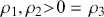 , so we can display outcomes in the positive quadrant of
 space, and assume equal numbers of all types (although it is interesting to consider more general populations as in, e.g., Wright Reference Wright1995). Figure 10 shows different regions labeled by
 to indicate different regimes that constitute equilibria.
Equilibrium set (panel (a)) and market structure (panel (b)) in Kiyotaki–Wright.
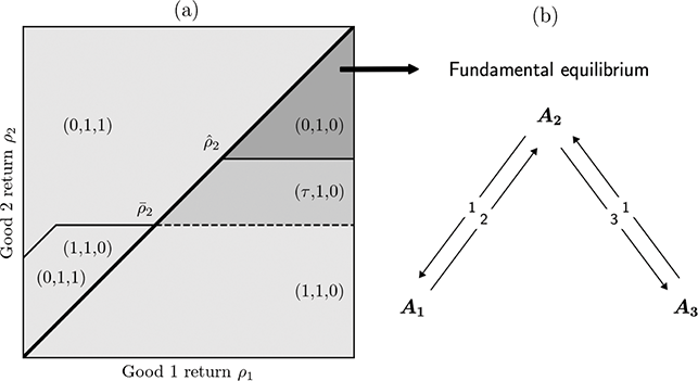
There are two cases, Model A or B, distinguished by
 or
or
 (this exhausts the possibilities since anything else would be a relabeling). In Figure 10, Model A corresponds to the region below the
 line, where there are two possibilities: If
 the unique outcome is
 ; and if
 it is
it is
 . To understand this, note that for
 good
good
 is more liquid than good
 since
since
 accepts good
 but not good
 , and
, and
 agents always have what
 wants. In contrast,
 agents always accept good
 but only have good
 with certain probability. Hence, good
 allows
 agents to consume sooner. If
 this liquidity factor does not compensate for a lower return; if
 it does. The reason
 is pivotal here is this: For
 , trading good
 for good
 enhances both liquidity and return, as does holding onto good
 for
for
 . Hence, only
 has a tradeoff.
In Model A,
 is called a fundamental equilibrium that has good
 as the universally accepted commodity money. It also has
 acting as middlemen – they acquire good
 from its producers and deliver it to its consumers – as shown in panel (b) of Figure 10 (see also Camera Reference Camera2001, who has endogenous intermediation using the same preference structure, but with divisible goods). This should remind readers of the market structure in Figure 2 from the Rubinstein–Wolinsky model.
However, if
 we instead get
 , called a speculative equilibrium, which has
 trading good
 for the lower-return good
 to improve their liquidity position, and both good
 and
and
 are used in indirect exchange. Theory delivers cutoffs for
 to sacrifice return for liquidity, but there is a gap: For
 there is no stationary, symmetric equilibrium in pure strategies, but one can show there is one in mixed strategies and nonstationary equilibria with
 cycling over time (Kehoe et al. Reference Kehoe and Levine1993).
Model B is similar, except that there is always an equilibrium in pure strategies, and for some
 s there are multiple equilibria in pure strategies. There can also be multiplicity for other configurations in mixed strategies for Models A and B. The coexistence of equilibria with different transactions patterns and liquidity properties shows that these are not necessarily pinned down by fundamentals.
Viewing Rubinstein–Wolinsky and Kiyotaki–Wright side by side reveals a connection between middlemen and money. Both arise in the presence of trade frictions, whether from search, information, commitment, etcetera. In these models, who trades with whom is central, something that is ignored in the classical, frictionless general equilibrium framework. In the models studied here, middlemen and money share economic concern: facilitating exchange. Despite these parallels, middlemen and money differ in other ways.Footnote 37 While the literature has advanced substantially on both topics in isolation, their interaction is an open area for research.
10 Other Contributions
We cannot present the details of all the interesting papers out there, but can provide a broad overview of some. Bose and Sengupta (Reference Bose and Sengupta2010) study a version where middlemen are immediately available to buyers and cater to repeat clientele. Tse (Reference Tse2011) has a setup where agents are dispersed over space and trading costs increase with distance, and shows that middlemen cluster at central locations, thereby increasing trade and welfare. Carapella and Monnet (Reference Carapella and Monnet2020) study how dealers help to reduce counterparty risk, while Gottardi et al. (Reference Gottardi, Maurin and Monnet2019) model counterparty plus asset risk under repo intermediation.
Some papers emphasize the difference between brokers and dealers: The former execute trades on behalf of others while the latter trade on their own behalf. In some models, middlemen set bid and ask prices, including Yavas (Reference Yavas1992), Spulber (Reference Spulber1996b), van Raalte and Webers (Reference Van Raalte and Webers1998), Rust and Hall (Reference Rust and Hall2003), Caillaud and Julien (Reference Caillaud and Julien2003), and Loertscher (Reference Loertscher2007). Spulber (Reference Spulber1996b) characterizes bid-ask spreads in a dynamic model. See also Yavas (Reference Yavas1994, Reference Yavas1996), which features brokers that get traders together, like real estate agents and employment agencies.
Another form of intermediation is the market-making platform, like Amazon, eBay, Uber, and Airbnb. These maintain a marketplace and take a commission in return. To understand this, Kultti et al. (Reference Kultti, Takalo and Vahamaa2021) consider endogenous platforms that coordinate meetings. Gautier et al. (Reference Gautier, Hu and Watanabe2023) model an agent’s decision to operate as a dealer, a platform, or both based on matching efficiency, inventory risk, and pricing power. Regarding matching efficiency, Teh et al. (Reference Teh, Wang and Watanabe2024) study platforms’ meeting algorithms in a directed search framework and show that limiting seller exposure to buyers can improve efficiency. Beyond market making, some platforms provide transaction and credit services, which is studied in Han et al. (2024)Footnote 38 and Hu et al. (2025).Footnote 39 Hagiu and Jullien (Reference Hagiu and Jullien2011) model intermediaries that divert consumer search, another role of platforms.
As middlemen play prominent roles in various industries, some papers try explicitly to capture specific institutional contexts rather than describing abstract, general models. Biglaiser et al. (Reference Biglaiser, Li, Murry and Zhao2020), for example, show how information asymmetries and assortative matching help explain empirical findings in used-car markets. Gavazza (Reference Gavazza2016) examines business aircraft, Leslie and Sorensen (Reference Leslie and Sorensen2014) study brokers of tickets to rock concerts, while Antras and Costinot (Reference Antras and Costinot2011) investigate the impact of middlemen in international trade. Afonso and Lagos (Reference Afonso and Lagos2015) and Bech and Monnet (Reference Bech and Monnet2016) model endogenous intermediation in interbank money markets. Geromichalos and Jung (Reference Geromichalos and Jung2018) study how intermediation affects bid-ask spreads and trade volume in the foreign exchange market.
In early papers, agent heterogeneity is highly stylized. Recent advancements push this boundary in several directions. Hugonnier et al. (Reference Hugonnier, Lester and Weill2022) allow arbitrary heterogeneity in flow payoffs and derive closed-form formulas for equilibrium outcomes. Uslu (Reference Üslü2019) has heterogeneity along three simultaneous dimensions – preferences, inventories, and arrival rates – and shows that the latter is the main driver of intermediation patterns. Bethune et al. (Reference Bethune, Sultanum and Trachter2022) model OTC markets where agents exhibit continuous heterogeneity in valuation and screening ability. Farboodi et al. (Reference Farboodi, Jarosch and Shimer2023) begin with ex ante identical agents and characterize continuous heterogeneity in equilibrium search intensity.
Although we focus mainly on models using a search theory, other approaches can also address the role of middlemen. Townsend (Reference Townsend1978) argues that multilateral trade is costly and thus intermediation emerges as a core allocation. Also examining core allocations, Kalai et al. (Reference Kalai, Postlewaite and Roberts1978) study market efficiency under coalitions connected by middlemen. Manea (Reference Manea2018) analyzes how network structure affects trade along different intermediation paths. Kotowski and Leister (Reference Kotowski and Leister2019) study network formation and show that free entry and competition may fail to eliminate redundant intermediaries. Chang and Zhang (2021)Footnote 40 model endogenous network hierarchy with implications for centrality and markups. Chiu et al. (Reference Chiu, Eisenschmidt and Monnet2020) and Farboodi (Reference Farboodi2023) model the interbank market and show that endogenous intermediation is a key determinant of the core–periphery network and equilibrium efficiency.
In summary, there is a great deal of good work in this area. While we cannot do justice to it all here, we have at least catalogued places where one can look for more.
11 Conclusion
This Element has presented various models and ideas in the economics literature using search and related tools to study middlemen. We focused on theory, neglecting empirical work in the interest of space, but there is certainly some good work on that and room for even more. One takeaway is that many interesting and tractable models have been developed, but there is also more that can be done in terms of theory. We hope this Element encourages further research.
Acknowledgments
We thank Chao Gu, Kohei Iwasaki, Yiting Li, Gary Biglaiser, Bo Hu, Makoto Watanabe, and Maryam Farboodi for input. We also thank two anonymous referees for very helpful comments. Gong acknowledges the support from the Natural Science Foundation of China (No.72503222), and the Humanities and Social Sciences Project of the Ministry of Education of China (No.24YJC790052). Wright acknowledges support from the Ray Zemon Chair in Liquid Assets and the Ken Burdett Professorship in Search Theory and Applications at University of Wisconsin-Madison. The usual disclaimers apply.
Chao Gu
University of Missouri
Chao Gu has been Professor at the University of Missouri since she graduated from Cornell University with a PhD in Economics in 2007. Her research interests are macroeconomics and monetary economics. She has published in top journals such as Econometrica, Journal of Political Economy, Review of Economic Studies, Journal of Monetary Economics, Journal of Economic Theory, and more.
Joseph Haslag
Auburn University
Joseph Haslag is the Donald Street Professor and Department Head in the Department of Economics at Auburn University. Before his appointment at Auburn, Dr. Haslag served in the Economics Departments at University of Missouri-Columbia, Michigan State University, Southern Methodist University and as a researcher at the Federal Reserve Bank of Dallas. He has written extensively on macroeconomic and monetary topics.
About the Series
This Element series is an outlet for current research on money, banking, payment systems and monetary policy. Elements in the series will consist of a combination of literature reviews and frontier research.