


1 Introduction
Enumeration reducibility (
 $\le _e$
) is a reducibility that captures the notion of how difficult it is to enumerate a given set of numbers. There are several definitions, but the one we find most useful in this article is the given by Friedberg and Rogers [Reference Friedberg and Rogers2] when they introduced the reducibility.
$\le _e$
) is a reducibility that captures the notion of how difficult it is to enumerate a given set of numbers. There are several definitions, but the one we find most useful in this article is the given by Friedberg and Rogers [Reference Friedberg and Rogers2] when they introduced the reducibility.
Definition 1.1. For sets
 $A,B\subseteq \omega $
we say that
$A,B\subseteq \omega $
we say that
 $A\le B$
if there is a c.e. set of axioms W such that
$A\le B$
if there is a c.e. set of axioms W such that
 $$ \begin{align*}n\in A\iff \exists u[\langle n, u \rangle \in W \land D_u \subseteq B].\end{align*} $$
Here
 $(D_u)_{u\in \omega }$
is the collection of all finite sets given by strong indexes.
$(D_u)_{u\in \omega }$
is the collection of all finite sets given by strong indexes.
One useful property of this definition is that it gives us a collection of enumeration operators
 $(\Psi _e)_{e\in \omega }$
. We define
$(\Psi _e)_{e\in \omega }$
. We define
 $A=\Psi _e(B)$
if
$A=\Psi _e(B)$
if
 $A\le _eB$
via the eth c.e. set
$A\le _eB$
via the eth c.e. set
 $W_e$
. Enumeration reducibility is a reducibility on the positive information about a set. This can be seen by the fact that if
$W_e$
. Enumeration reducibility is a reducibility on the positive information about a set. This can be seen by the fact that if
 $A\subseteq B$
then
$A\subseteq B$
then
 $\Psi _e(A)\subseteq \Psi _e(B)$
.
$\Psi _e(A)\subseteq \Psi _e(B)$
.
Enumeration reducibility is a pre-order and the equivalence classes form an upper semi-lattice
 $\mathcal {D}_e$
with least element
$\mathcal {D}_e$
with least element
 $\mathbf {0}_e$
, consisting of all c.e. sets, and joins given by the usual operation. There is also an enumeration jump given by
$\mathbf {0}_e$
, consisting of all c.e. sets, and joins given by the usual operation. There is also an enumeration jump given by
 $A\mapsto \bigoplus _{e\in \omega } \Psi _e(A) \oplus \bigoplus _{e\in \omega } \overline {\Psi _e(A)}$
. Like with the Turing jump we have that
$A\mapsto \bigoplus _{e\in \omega } \Psi _e(A) \oplus \bigoplus _{e\in \omega } \overline {\Psi _e(A)}$
. Like with the Turing jump we have that
 $A<_e A'$
.
$A<_e A'$
.
One aspect of enumeration reducibility that has been well studied is its relationship with Turing reducibility. The Turing degrees embed into the enumeration degrees via the map induced by
 $A\mapsto A\oplus \overline {A}$
. This follows from the fact that
$A\mapsto A\oplus \overline {A}$
. This follows from the fact that
 $A\oplus \overline {A}\le _e B\oplus \overline {B}\iff A\le _T B$
. This embedding is known to be a proper embedding [Reference Medvedev9], and the Turing and enumeration jump coincide on these degrees. The image of the Turing degrees is known as the total degrees.
$A\oplus \overline {A}\le _e B\oplus \overline {B}\iff A\le _T B$
. This embedding is known to be a proper embedding [Reference Medvedev9], and the Turing and enumeration jump coincide on these degrees. The image of the Turing degrees is known as the total degrees.
Definition 1.2. We say that a set A is total if
 $\overline {A}\le _eA$
. We say that A is cototal if
$\overline {A}\le _eA$
. We say that A is cototal if
 $A\le _e \overline {A}$
. A degree is total (cototal) if it contains a total (cototal) set.
$A\le _e \overline {A}$
. A degree is total (cototal) if it contains a total (cototal) set.
It is known that the total degrees are a proper subclass of the cototal degrees and that the cototal degrees are a proper subclass of all enumeration degrees [Reference Andrews, Ganchev, Kuyper, Lempp, Miller, Soskova and Soskova1]. It is known that both the jump [Reference Kalimullin7] and the total degrees [Reference Ganchev and Soskova3] are definable within the structure
 $(\mathcal {D}_e, \le _e)$
.
$(\mathcal {D}_e, \le _e)$
.
While there are many similarities between these classes of degrees they are structurally different. One notable difference is the fact that, while there are minimal Turing degrees, Gutteridge [Reference Gutteridge5] proved that the enumeration degrees are downwards dense.
We have seen that Turing reducibility can be defined in terms of enumeration reducibility. An important early result of Selman [Reference Selman12] shows how to define enumeration reducibility in terms of Turing reducibility.
Theorem 1.3 (Selman’s theorem)
 $A\le _e B$
if and only if, for all X if
$A\le _e B$
if and only if, for all X if
 $B\le _e X\oplus \overline {X}$
then
$B\le _e X\oplus \overline {X}$
then
 $A\le _e X\oplus \overline {X}$
.
$A\le _e X\oplus \overline {X}$
.
This theorem states that an enumeration degree is uniquely determined by total degrees above it. This means that the total degrees form an automorphism base for the enumeration degrees.
Sanchis [Reference Sanchis11] introduced the notion of hyperenumeration reducibility
 $\le _{he}$
, an analogue of enumeration reducibility relating to hyperarithmetic reducibility rather than Turing reducibility.
$\le _{he}$
, an analogue of enumeration reducibility relating to hyperarithmetic reducibility rather than Turing reducibility.
Definition 1.4 (Sanchis [Reference Sanchis11])
We say that
 $A\le _{he} B$
if there is a c.e. set W such that
$A\le _{he} B$
if there is a c.e. set W such that
 $$ \begin{align*}n\in A \iff \forall f\in \omega^\omega \exists u\in \omega, x\prec f [\langle n, x, u\rangle \in W \land D_u\subseteq B].\end{align*} $$
Sanchis proved that
 $\le _{he}$
is a pre-order giving rise to the hyperenumeration degrees
$\le _{he}$
is a pre-order giving rise to the hyperenumeration degrees
 $\mathcal {D}_{he}$
and proved that the map
$\mathcal {D}_{he}$
and proved that the map
 $A\mapsto A\oplus \overline {A}$
induces an embedding of the hyperarithmetic degrees into the hyperenumeration degrees. The main result of Sanchis’ paper was proving that there is a hyperenumeration degree that is not in the image of this embedding. In keeping with the notion of total degrees in the enumeration degrees we call the degrees in the image of this embedding the hypertotal degrees.
$A\mapsto A\oplus \overline {A}$
induces an embedding of the hyperarithmetic degrees into the hyperenumeration degrees. The main result of Sanchis’ paper was proving that there is a hyperenumeration degree that is not in the image of this embedding. In keeping with the notion of total degrees in the enumeration degrees we call the degrees in the image of this embedding the hypertotal degrees.
Definition 1.5. We say that a set A is hypertotal if
 $\overline {A}\le _{he}A$
. We say that A is hypercototal if
$\overline {A}\le _{he}A$
. We say that A is hypercototal if
 $A\le _{he} \overline {A}$
. A degree is hypertotal (hypercototal) if it contains a hypertotal (hypercototal) set.
$A\le _{he} \overline {A}$
. A degree is hypertotal (hypercototal) if it contains a hypertotal (hypercototal) set.
In this article we look at a couple of the aspects of the relationships between Turing reducibility and enumeration reducibility and see if they also hold for the relationship between hyperarithmetic reducibility and hyperenumeration reducibility. In Section 3 we show that Selman’s theorem fails for hyperenumeration reducibility. The proof of this works by constructing a uniformly e-pointed tree without dead ends that is not of hypertotal degree.
E-pointed trees were introduced by McCarthy [Reference McCarthy8] and were used to characterize the cototal enumeration degrees.
Definition 1.6. A tree T is e-pointed if, for every path
 $P\in [T]$
, we have that T is c.e. in P. We say that T is uniformly e-pointed if there is a single operator
$P\in [T]$
, we have that T is c.e. in P. We say that T is uniformly e-pointed if there is a single operator
 $\Psi _e$
such that for all paths
$\Psi _e$
such that for all paths
 $P\in [T]$
we have
$P\in [T]$
we have
 $T=\Psi _e(P)$
.
$T=\Psi _e(P)$
.
McCarthy proved that the degree of a uniformly e-pointed tree on
 $2^{<\omega }$
is a cototal set, and characterized the cototal degrees as the degrees of uniformly e-pointed trees on
$2^{<\omega }$
is a cototal set, and characterized the cototal degrees as the degrees of uniformly e-pointed trees on
 $2^{<\omega }$
without dead ends and as the degrees of general e-pointed trees on
$2^{<\omega }$
without dead ends and as the degrees of general e-pointed trees on
 $2^{<\omega }$
.
$2^{<\omega }$
.
Goh et al. [Reference Le Goh, Jacobsen-Grocott, Miller and Soskova4] and Jacobsen-Grocott [Reference Jacobsen-Grocott6] have studied e-pointed trees on
 $\omega ^{<\omega }$
. They found some interesting connections to hyperenumeration reducibility and the notion of hypercototality. They proved that every uniformly e-pointed tree is hypercototal and that the enumeration degrees of these trees are the same as the degrees of hypercototal sets and the same as the degrees of general e-pointed trees.
$\omega ^{<\omega }$
. They found some interesting connections to hyperenumeration reducibility and the notion of hypercototality. They proved that every uniformly e-pointed tree is hypercototal and that the enumeration degrees of these trees are the same as the degrees of hypercototal sets and the same as the degrees of general e-pointed trees.
They found that when considering e-pointed trees on
 $\omega ^{<\omega }$
without dead ends things become different. They proved that there is an arithmetic set that is not enumeration equivalent to any e-pointed tree without a dead end. They also proved that there is a uniformly e-pointed tree without dead ends is not of cototal enumeration degree.
$\omega ^{<\omega }$
without dead ends things become different. They proved that there is an arithmetic set that is not enumeration equivalent to any e-pointed tree without a dead end. They also proved that there is a uniformly e-pointed tree without dead ends is not of cototal enumeration degree.
In Section 3 we prove a stronger separation.
Theorem 1.7. There is a uniformly e-pointed tree
 $T^{\mathcal {G}}\subseteq \omega ^{<\omega }$
with no dead ends such that
$T^{\mathcal {G}}\subseteq \omega ^{<\omega }$
with no dead ends such that
 $T^{\mathcal {G}}$
is not hypertotal.
$T^{\mathcal {G}}$
is not hypertotal.
This has some interesting corollaries, one of which is the failure of Selman’s theorem for hyperenumeration reducibility.
Corollary 1.8. There are sets
 $A,B$
such that
$A,B$
such that
 $B\nleq _{he} A$
and for any X, if
$B\nleq _{he} A$
and for any X, if
 $A\le _{he}X\oplus \overline {X}$
then
$A\le _{he}X\oplus \overline {X}$
then
 $B\le _{he} X\oplus \overline {X}$
.
$B\le _{he} X\oplus \overline {X}$
.
This is one way in which hyperenumeration reducibility is different from enumeration reducibility. In Section 4 we prove that, like the enumeration degrees, the hyperenumeration degrees are downwards dense, giving another example of how these degree structures are similar. We prove this by adapting Gutteridge’s original proof, however we discover that, in general, priority arguments that work for the enumeration degrees will not work for the hyperenumeration degrees. We give an explanation of this issue in Section 4 and describe a tool that can work is some cases.
In Section 5 we look at some other natural reducibilities that could be considered hyperarithmetic analogues of enumeration reducibility, and we consider their relationship to hyperarithmetic reducibility and enumeration reducibility.
2 Preliminaries
Some basic points of notation. We use
 $n,m,i,j,k$
for natural numbers. We use
$n,m,i,j,k$
for natural numbers. We use
 $\alpha ,\beta ,\gamma $
for ordinals. We use
$\alpha ,\beta ,\gamma $
for ordinals. We use
 $\sigma ,\tau ,\rho ,\upsilon ,x,y,z$
to represent strings of natural numbers.
$\sigma ,\tau ,\rho ,\upsilon ,x,y,z$
to represent strings of natural numbers.
 $\langle \sigma \rangle $
corresponds to the Gödel number of the string
$\langle \sigma \rangle $
corresponds to the Gödel number of the string
 $\sigma $
. We use T and S to refer to trees in
$\sigma $
. We use T and S to refer to trees in
 $\omega ^{<\omega }$
. We will give a brief overview of some of the tools of higher computability theory that we will use in this article. A more in depth introduction to higher computability can be found in Sacks’ book [Reference Sacks10].
$\omega ^{<\omega }$
. We will give a brief overview of some of the tools of higher computability theory that we will use in this article. A more in depth introduction to higher computability can be found in Sacks’ book [Reference Sacks10].
2.1 Hyperenumeration reducibility
It is useful to define enumeration reducibility in terms of operators
 $(\Psi _e)_{e\in \omega }$
. Using Definition 1.4 we can define hyperenumeration operators
$(\Psi _e)_{e\in \omega }$
. Using Definition 1.4 we can define hyperenumeration operators
 $(\Gamma _e)_{e\in \omega }$
in a similar way.
$(\Gamma _e)_{e\in \omega }$
in a similar way.
Definition 2.1. For the eth c.e. set
 $W_e$
we define the hyperenumeration operators
$W_e$
we define the hyperenumeration operators
 $\Gamma _e$
by
$\Gamma _e$
by
 $n\in \Gamma _e(A)\iff \forall f\in \omega ^\omega \exists \sigma \preceq f, u\in \omega [ \langle n, \sigma , u\rangle \in W_e\land D_u\subseteq A]$
.
$n\in \Gamma _e(A)\iff \forall f\in \omega ^\omega \exists \sigma \preceq f, u\in \omega [ \langle n, \sigma , u\rangle \in W_e\land D_u\subseteq A]$
.
Now we examine the relationship between
 $\Gamma _e$
and
$\Gamma _e$
and
 $\Psi _e$
. Both use the same set
$\Psi _e$
. Both use the same set
 $W_e$
in their definition. Consider the tree
$W_e$
in their definition. Consider the tree
 $S_e^A$
defined by
$S_e^A$
defined by ![]() . From the definition of
. From the definition of
 $\Gamma _e$
, we have that
$\Gamma _e$
, we have that
 $n\in \Gamma _e(A)$
if and only if
$n\in \Gamma _e(A)$
if and only if
 $S_e^A$
does not have an infinite path starting with n. We have that
$S_e^A$
does not have an infinite path starting with n. We have that
 $S_e^A\le _e \overline {A}$
and
$S_e^A\le _e \overline {A}$
and
 $\overline {S_e^A}\le _e A$
.
$\overline {S_e^A}\le _e A$
.
The form of
 $S_e^A$
inspires us to come up with the notion of a hyperenumeration of a set.
$S_e^A$
inspires us to come up with the notion of a hyperenumeration of a set.
Definition 2.2. We say that a tree S is a hyperenumeration of a set B if
 ${B= \{n: \forall f\in [S](f(0)\ne n)\}}$
.
${B= \{n: \forall f\in [S](f(0)\ne n)\}}$
.
From this we have that
 $B\le _{he}\overline {S}$
via the same operator for every hyperenumeration S of B. By coding a set X into a layer of
$B\le _{he}\overline {S}$
via the same operator for every hyperenumeration S of B. By coding a set X into a layer of
 $S_e^X$
, we have that for every X such that B is
$S_e^X$
, we have that for every X such that B is
 $\Pi ^1_1$
in X, there is a hyperenumeration S of B such that
$\Pi ^1_1$
in X, there is a hyperenumeration S of B such that
 $S\equiv _T X$
. So the hyperenumerations of B characterize the hypertotal degrees above
$S\equiv _T X$
. So the hyperenumerations of B characterize the hypertotal degrees above
 $\deg _{he}(B)$
much like how the enumerations of B characterize the total e-degrees above the
$\deg _{he}(B)$
much like how the enumerations of B characterize the total e-degrees above the
 $\deg _e(B)$
.
$\deg _e(B)$
.
While the notation is a little different, Sanchis [Reference Sanchis11] used a similar idea when proving the existence of a non-hypertotal degree.
Sanchis proved some other results about hyperenumeration reducibility that we will use in this article.
Lemma 2.3 (Sanchis [Reference Sanchis11])
For sets
 $A,B\subseteq \omega $
we have the following:
$A,B\subseteq \omega $
we have the following:
-
1. If there is a
 $\Pi ^1_1$
set V such that then
$A\le _{he} B$
.
$\Pi ^1_1$
set V such that then
$A\le _{he} B$
. -
2. If
$A\le _e B$
then
$A\le _{he} B$
and
$\overline {A}\le _{he} \overline {B}$
.


2.2 Admissible sets and higher computability theory
The usual definition of a
 $\Pi _1^1$
set of natural numbers is a set of the form
$\Pi _1^1$
set of natural numbers is a set of the form
 $m\in X\iff \forall f\in \omega ^\omega \exists n [R(f,n,m)]$
where R is a computable relation. However admissibility gives us another definition in terms of
$m\in X\iff \forall f\in \omega ^\omega \exists n [R(f,n,m)]$
where R is a computable relation. However admissibility gives us another definition in terms of
 $L_{\omega _1^{{CK}}}$
that is useful.
$L_{\omega _1^{{CK}}}$
that is useful.
Definition 2.4. A set M is admissible if it is transitive, closed under union, pairing, and Cartesian product as well as satisfying the following two properties:
-
Δ1 -comprehension: For every
$\Delta _1$
definable class
$A\subseteq M$
and set
$a\in M$
the set
$A\cap a\in M$
. -
Σ1 -collection: For every
$\Sigma _1$
definable class relation
$R\subseteq M^2$
and set
$a\in M$
such that
$a\subseteq \mathrm {dom}(R)$
there is
$b\in M$
such that
$a= R^{-1}[b]$
.


The smallest admissible set is
 $\mathrm {HF}$
, the collection of hereditarily finite sets. Looking at the
$\mathrm {HF}$
, the collection of hereditarily finite sets. Looking at the
 $\Delta _1$
and
$\Delta _1$
and
 $\Sigma _1$
subsets of
$\Sigma _1$
subsets of
 $\mathrm {HF}$
is one notion of computability. We have that the
$\mathrm {HF}$
is one notion of computability. We have that the
 $\Delta _1$
subsets of
$\Delta _1$
subsets of
 $\mathrm {HF}$
are computable sets and the
$\mathrm {HF}$
are computable sets and the
 $\Sigma _1$
subsets of
$\Sigma _1$
subsets of
 $\mathrm {HF}$
are the c.e. sets. We generalize this to an arbitrary admissible set M by calling a set
$\mathrm {HF}$
are the c.e. sets. We generalize this to an arbitrary admissible set M by calling a set
 $A\subseteq M M$
-computable if it is a
$A\subseteq M M$
-computable if it is a
 $\Delta _1$
subset of M and M-c.e. if it is a
$\Delta _1$
subset of M and M-c.e. if it is a
 $\Sigma _1$
subset of M.
$\Sigma _1$
subset of M.
The smallest admissible set containing
 $\omega $
is
$\omega $
is
 $L_{\omega _1^{{CK}}}$
. We have that the
$L_{\omega _1^{{CK}}}$
. We have that the
 $L_{\omega _1^{{CK}}}$
-c.e. subsets of
$L_{\omega _1^{{CK}}}$
-c.e. subsets of
 $\omega $
are precisely the
$\omega $
are precisely the
 $\Pi ^1_1$
sets. This means that the
$\Pi ^1_1$
sets. This means that the
 $L_{\omega _1^{{CK}}}$
-computable subsets of
$L_{\omega _1^{{CK}}}$
-computable subsets of
 $\omega $
sets are the hyperarithmetic sets. Note that
$\omega $
sets are the hyperarithmetic sets. Note that
 $\Delta _1$
-comprehension means that the hyperarithmetic sets are precisely the sets in
$\Delta _1$
-comprehension means that the hyperarithmetic sets are precisely the sets in
 $\mathcal {P}(\omega )\cap L_{\omega _1^{{CK}}}$
.
$\mathcal {P}(\omega )\cap L_{\omega _1^{{CK}}}$
.
These results about
 $\Pi ^1_1$
and hyperarithmetic sets can be relativized for some set X. We define
$\Pi ^1_1$
and hyperarithmetic sets can be relativized for some set X. We define
 $L_X$
to be the smallest admissible set containing X. We have that
$L_X$
to be the smallest admissible set containing X. We have that
 $A\subseteq \omega $
is
$A\subseteq \omega $
is
 $\Pi ^1_1$
in X if and only if it is
$\Pi ^1_1$
in X if and only if it is
 $L_X$
-c.e. and hyperarithmetic in X if and only if
$L_X$
-c.e. and hyperarithmetic in X if and only if
 $A\in L_X$
. Note that while we have
$A\in L_X$
. Note that while we have
 $\mathrm {ORD}^{L_X}=\omega _1^X$
and
$\mathrm {ORD}^{L_X}=\omega _1^X$
and
 $L_{\omega _1^X}\subseteq L_X$
it is only sometimes the case that
$L_{\omega _1^X}\subseteq L_X$
it is only sometimes the case that
 $L_X=L_{\omega _1^X}$
.
$L_X=L_{\omega _1^X}$
.
2.3 Some facts about trees
We will deal a lot with trees in this chapter so it is useful to have operations on trees. For a tree
 $S\subseteq \omega ^{<\omega }$
and string x we define
$S\subseteq \omega ^{<\omega }$
and string x we define
 $\mathrm {Ext}(S, x)$
to be the tree of extensions of x.
$\mathrm {Ext}(S, x)$
to be the tree of extensions of x. ![]() . A relation on trees that we will use is
. A relation on trees that we will use is
 $\preceq $
. We say
$\preceq $
. We say
 $T\preceq S$
if S is an end extension of T. That is,
$T\preceq S$
if S is an end extension of T. That is,
 $T\subseteq S$
and for all
$T\subseteq S$
and for all
 $\sigma \in S$
the longest initial segment of
$\sigma \in S$
the longest initial segment of
 $\sigma $
that is in T is a leaf in T.
$\sigma $
that is in T is a leaf in T.
Now we define
 $\mathrm {rank}(S)$
for a well founded tree S using transfinite recursion. We define
$\mathrm {rank}(S)$
for a well founded tree S using transfinite recursion. We define
 $\mathrm {rank}(\emptyset )=0$
. Given a tree S we define
$\mathrm {rank}(\emptyset )=0$
. Given a tree S we define
 $\mathrm {rank}(S)=\sup _{i\in S} \mathrm {rank}(\mathrm {Ext}(S, i))+1$
.
$\mathrm {rank}(S)=\sup _{i\in S} \mathrm {rank}(\mathrm {Ext}(S, i))+1$
.
As it turns out, this function
 $\mathrm {rank}$
is in fact
$\mathrm {rank}$
is in fact
 $L_{\omega _1^{{CK}}}$
-partial computable, i.e., its graph is
$L_{\omega _1^{{CK}}}$
-partial computable, i.e., its graph is
 $L_{\omega _1^{{CK}}}$
-c.e. To help the reader feel more familiar with computability on
$L_{\omega _1^{{CK}}}$
-c.e. To help the reader feel more familiar with computability on
 $L_{\omega _1^{{CK}}}$
we include a sketch of the proof of this fact.
$L_{\omega _1^{{CK}}}$
we include a sketch of the proof of this fact.
For a tree
 $T\in L_{\omega _1^{{CK}}}$
and function
$T\in L_{\omega _1^{{CK}}}$
and function
 $f\in L_{\omega _1^{{CK}}}$
we say that f is a rank function on T if
$f\in L_{\omega _1^{{CK}}}$
we say that f is a rank function on T if
 $\mathrm {dom}(f)=T$
,
$\mathrm {dom}(f)=T$
,
 $\mathrm {range}(f)\subseteq {\omega _1^{{CK}}}$
, for each leaf
$\mathrm {range}(f)\subseteq {\omega _1^{{CK}}}$
, for each leaf
 $x\in T$
we have
$x\in T$
we have
 $f(x)=1$
and for each non-leaf
$f(x)=1$
and for each non-leaf
 $y\in T$
we have that
$y\in T$
we have that ![]() . Since the quantifies are all bounded it is
. Since the quantifies are all bounded it is
 $L_{\omega _1^{{CK}}}$
-computable to check if f is a rank function on T. If f is a rank function on T then f is unique and
$L_{\omega _1^{{CK}}}$
-computable to check if f is a rank function on T. If f is a rank function on T then f is unique and
 $f(\emptyset )=\mathrm {rank}(T)$
. So we can define
$f(\emptyset )=\mathrm {rank}(T)$
. So we can define
 $\mathrm {rank}$
by
$\mathrm {rank}$
by
 $\mathrm {rank}(T) =\alpha $
if there is a rank function f on T such that
$\mathrm {rank}(T) =\alpha $
if there is a rank function f on T such that
 $f(\emptyset )=\alpha $
or
$f(\emptyset )=\alpha $
or
 $\alpha =0$
and
$\alpha =0$
and
 $T=\emptyset $
. So we now have a
$T=\emptyset $
. So we now have a
 $\Sigma _1$
definition of
$\Sigma _1$
definition of
 $\mathrm {rank}$
. The only problem is that its domain may not consist of all well founded trees
$\mathrm {rank}$
. The only problem is that its domain may not consist of all well founded trees
 $T\in L_{\omega _1^{{CK}}}$
.
$T\in L_{\omega _1^{{CK}}}$
.
To prove that the domain of
 $\mathrm {rank}$
is all well founded trees in
$\mathrm {rank}$
is all well founded trees in
 $L_{\omega _1^{{CK}}}$
we use induction on the true rank of T (i.e., T’s rank according to V as we do not yet know that T has rank in
$L_{\omega _1^{{CK}}}$
we use induction on the true rank of T (i.e., T’s rank according to V as we do not yet know that T has rank in
 $L_{\omega _1^{{CK}}}$
). Suppose all trees of rank less than T are in the domain of rank. Then for each
$L_{\omega _1^{{CK}}}$
). Suppose all trees of rank less than T are in the domain of rank. Then for each
 $i\in T$
there is a rank function
$i\in T$
there is a rank function
 $f_i$
for
$f_i$
for
 $\mathrm {Ext}(T, i)$
. Since the map,
$\mathrm {Ext}(T, i)$
. Since the map,
 $S\mapsto f$
where f is the rank function on S, is
$S\mapsto f$
where f is the rank function on S, is
 $L_{\omega _1^{{CK}}}$
-c.e,
$L_{\omega _1^{{CK}}}$
-c.e,
 $\Sigma _1$
-collection tells us that the map
$\Sigma _1$
-collection tells us that the map
 $i\mapsto f_i$
is in
$i\mapsto f_i$
is in
 $L_{\omega _1^{{CK}}}$
. So we can build a rank function
$L_{\omega _1^{{CK}}}$
. So we can build a rank function
 $f\in L_{\omega _1^{{CK}}}$
on T by
$f\in L_{\omega _1^{{CK}}}$
on T by ![]() and
and
 $f(\emptyset )=\sup _{i\in T} f_i(\emptyset )+1$
.
$f(\emptyset )=\sup _{i\in T} f_i(\emptyset )+1$
.
One nice result of this is that if a tree
 $T\in L_{\omega _1^{{CK}}}$
is well founded, then it has rank
$T\in L_{\omega _1^{{CK}}}$
is well founded, then it has rank
 $<{\omega _1^{{CK}}}$
and the set of all well founded trees in
$<{\omega _1^{{CK}}}$
and the set of all well founded trees in
 $L_{\omega _1^{{CK}}}$
is
$L_{\omega _1^{{CK}}}$
is
 $L_{\omega _1^{{CK}}}$
-c.e. This could also be seen by observing that trees in
$L_{\omega _1^{{CK}}}$
-c.e. This could also be seen by observing that trees in
 $L_{\omega _1^{{CK}}}$
are
$L_{\omega _1^{{CK}}}$
are
 $\Delta _0$
definable and so hyperarithmetic.
$\Delta _0$
definable and so hyperarithmetic.
3 A uniformly e-pointed tree in
$\omega ^\omega $
without dead ends that is not of hyper total degree

In this section we prove the following theorem.
Theorem 3.1. There is a uniformly e-pointed tree
 $T^{\mathcal {G}}\subseteq \omega ^{<\omega }$
with no dead ends such that
$T^{\mathcal {G}}\subseteq \omega ^{<\omega }$
with no dead ends such that
 $T^{\mathcal {G}}$
is not hypertotal.
$T^{\mathcal {G}}$
is not hypertotal.
3.1 The forcing partial order
We will be using a similar forcing to the one used in [Reference Le Goh, Jacobsen-Grocott, Miller and Soskova4] to construct a uniformly e-pointed tree that is not of introenumerable degree.
Let
 $\{T_\sigma :\sigma \in \omega ^{<\omega }\}$
be an effective listing of all finite trees in
$\{T_\sigma :\sigma \in \omega ^{<\omega }\}$
be an effective listing of all finite trees in
 $\omega ^{<\omega }$
where for each
$\omega ^{<\omega }$
where for each
 $\sigma \in \omega ^{<\omega }$
the sequence
$\sigma \in \omega ^{<\omega }$
the sequence ![]() lists each finite tree that contains
lists each finite tree that contains
 $T_\sigma $
infinitely often. We will define the reduction
$T_\sigma $
infinitely often. We will define the reduction
 $\Psi $
by which our tree will be e-pointed as
$\Psi $
by which our tree will be e-pointed as
 $\Psi (p)= \bigcup _{n\in \omega } T_{p{\restriction } n}$
.
$\Psi (p)= \bigcup _{n\in \omega } T_{p{\restriction } n}$
.
We define a condition to be some
 $p=(T^p,L^p:T^p\times T^p\rightarrow {\omega _1^{{CK}}})\in L_{\omega _1^{{CK}}}$
where the following hold:
$p=(T^p,L^p:T^p\times T^p\rightarrow {\omega _1^{{CK}}})\in L_{\omega _1^{{CK}}}$
where the following hold:
-
1.
$T^p\subseteq \omega ^{<\omega }$
is a well founded tree. -
2. For each
$\sigma \in T^p$
we have that
$ T_\sigma \subseteq T^p$
. -
3. For each
$\sigma ,\tau \in T^p$
we have that
$L^p(\sigma ,\tau )=0$
if and only if
$\sigma \in T_\tau $
. -
4. If
$\sigma \in T^p$
and
$\rho \prec \tau \in T^p$
then
$L^p(\sigma ,\tau )=0$
or
$L^p(\sigma ,\tau )<L^p(\sigma ,\rho )$
. -
5. For each
$\tau \in T^p$
and
$n<\omega $
the set
$\{\sigma : L^p(\sigma ,\tau )\le n\}$
is finite.


Rules 1 and 2 are there to ensure that our conditions have not defined the full tree. The purpose of L is to ensure that each node is eventually enumerated along each path. We can think of
 $L^p(\sigma ,\tau )=\alpha $
as promising that within
$L^p(\sigma ,\tau )=\alpha $
as promising that within
 $\alpha $
many steps along an extension of
$\alpha $
many steps along an extension of
 $\tau $
we will enumerate
$\tau $
we will enumerate
 $\sigma $
.
$\sigma $
.
For two conditions p and q we say
 $p\le q$
if
$p\le q$
if
 $T^q\preceq T^p$
and
$T^q\preceq T^p$
and
 $L^q\subseteq L^p$
. For a filter
$L^q\subseteq L^p$
. For a filter
 $\mathcal {G}$
we define
$\mathcal {G}$
we define
 $T^{\mathcal {G}}=\bigcup _{p\in \mathcal {G}}T^p$
. The fact that we must have
$T^{\mathcal {G}}=\bigcup _{p\in \mathcal {G}}T^p$
. The fact that we must have
 $T^q\preceq T^p$
means that if
$T^q\preceq T^p$
means that if
 $p\in \mathcal {G}$
,
$p\in \mathcal {G}$
,
 $\sigma $
is not a leaf in
$\sigma $
is not a leaf in
 $T^p$
and
$T^p$
and ![]() then
then ![]() . So we have a way of forcing strings into the complement of
. So we have a way of forcing strings into the complement of
 $T^{\mathcal {G}}$
.
$T^{\mathcal {G}}$
.
Proposition 3.2. The set of conditions is
 $L_{\omega _1^{{CK}}}$
-c.e. and the relation
$L_{\omega _1^{{CK}}}$
-c.e. and the relation
 $\le $
on conditions is
$\le $
on conditions is
 $L_{\omega _1^{{CK}}}$
-computable.
$L_{\omega _1^{{CK}}}$
-computable.
Proof. Properties 2–5 are all straightforwardly
 $\Delta _1$
conditions. To check if a tree T is well founded we ask if there is a rank function
$\Delta _1$
conditions. To check if a tree T is well founded we ask if there is a rank function
 $f\in L$
such that
$f\in L$
such that
 $f(\sigma )=\mathrm {rank}(\mathrm {Ext}(T, \sigma ))$
, so a
$f(\sigma )=\mathrm {rank}(\mathrm {Ext}(T, \sigma ))$
, so a
 $\Sigma _1$
question. So property 1 is a
$\Sigma _1$
question. So property 1 is a
 $\Sigma _1$
condition. Hence the set of valid conditions is
$\Sigma _1$
condition. Hence the set of valid conditions is
 $L_{\omega _1^{{CK}}}$
-c.e.
$L_{\omega _1^{{CK}}}$
-c.e.
 $q\le p$
is clearly
$q\le p$
is clearly
 $\Delta _0$
so
$\Delta _0$
so
 $\le $
is an
$\le $
is an
 $L_{\omega _1^{{CK}}}$
-computable relation with
$L_{\omega _1^{{CK}}}$
-computable relation with
 $L_{\omega _1^{{CK}}}$
-c.e. domain.
$L_{\omega _1^{{CK}}}$
-c.e. domain.
Proposition 3.3. For a condition p we have ![]() for all
for all
 $\sigma ,\tau \in T^p$
.
$\sigma ,\tau \in T^p$
.
Proof. We will use induction on
 $L^p(\sigma ,\tau )$
. Base case,
$L^p(\sigma ,\tau )$
. Base case,
 $L^p(\sigma ,\tau )=0$
. Then
$L^p(\sigma ,\tau )=0$
. Then
 $\sigma \in T_\tau $
so
$\sigma \in T_\tau $
so ![]() and
and
 $\mathrm {rank}(\emptyset )=0$
. Now suppose the proposition holds for all
$\mathrm {rank}(\emptyset )=0$
. Now suppose the proposition holds for all
 $\beta <\alpha $
and
$\beta <\alpha $
and
 $L^p(\sigma ,\tau )=\alpha $
. Then we have for each
$L^p(\sigma ,\tau )=\alpha $
. Then we have for each ![]() we have
we have ![]() by induction hypothesis. By property 4 and definition of
by induction hypothesis. By property 4 and definition of
 $\mathrm {rank}$
we have
$\mathrm {rank}$
we have  .
.
In order for this forcing notion to have nontrivial generics we need a way to extend conditions. Fix a condition p. Let
 $A\subseteq \omega ^{<\omega }$
be a set such that for all
$A\subseteq \omega ^{<\omega }$
be a set such that for all ![]() we have
we have
 $\sigma \in T^p$
and
$\sigma \in T^p$
and ![]() . For such an A we can define
. For such an A we can define
 $q=p[A]$
by
$q=p[A]$
by
 $T^{q}=T^p\cup A$
and
$T^{q}=T^p\cup A$
and
 $L^{q}$
given by
$L^{q}$
given by

Lemma 3.4. If A meets the requirement of the definition then
 $p[A]$
is a valid condition. If we also have that
$p[A]$
is a valid condition. If we also have that
 $T^p\preceq T^p\cup A$
then
$T^p\preceq T^p\cup A$
then
 $p[A]\le p$
.
$p[A]\le p$
.
Proof. We show that
 $q=p[A]$
is well defined. Our requirement for A ensures that 1 and 2 hold. For 3–5, since
$q=p[A]$
is well defined. Our requirement for A ensures that 1 and 2 hold. For 3–5, since
 $L^p=L^q\restriction T^p\times T^p$
the only way we can run into a problem is when considering
$L^p=L^q\restriction T^p\times T^p$
the only way we can run into a problem is when considering ![]() . If
. If
 $\rho \prec \tau \in T^q$
then by definition
$\rho \prec \tau \in T^q$
then by definition ![]() . If
. If ![]() then
then
 $L^p(\tau ,\rho )\ge L^p(\tau , \sigma )$
. If
$L^p(\tau ,\rho )\ge L^p(\tau , \sigma )$
. If
 $0<L^p(\tau , {\sigma })<\omega $
then
$0<L^p(\tau , {\sigma })<\omega $
then ![]() . If
. If
 $L^p(\tau , {\sigma })\ge \omega $
then
$L^p(\tau , {\sigma })\ge \omega $
then ![]() . So 4 holds.
. So 4 holds.
Fix n and
 $\tau $
and consider the set
$\tau $
and consider the set
 $\{\rho : L^q(\rho ,\tau )\le n\}$
. If
$\{\rho : L^q(\rho ,\tau )\le n\}$
. If
 $\tau \in T^p$
then we have added at most n many elements to the set, so it is still finite. If
$\tau \in T^p$
then we have added at most n many elements to the set, so it is still finite. If ![]() and
and
 $\rho $
is in this set then either
$\rho $
is in this set then either
 $\rho $
belongs to the finite set
$\rho $
belongs to the finite set
 $\{\rho : L^p(\rho ,{\sigma })\le n+1\}$
or
$\{\rho : L^p(\rho ,{\sigma })\le n+1\}$
or
 $\langle \rho \rangle \le n$
. So there are only finitely many
$\langle \rho \rangle \le n$
. So there are only finitely many
 $\rho $
that can be in
$\rho $
that can be in
 $\{\rho : L^q(\rho ,\tau )\le n\}$
. So 5 holds.
$\{\rho : L^q(\rho ,\tau )\le n\}$
. So 5 holds.
Now consider the set
 $\{\rho : L^q(\rho ,\tau )=0\}$
. If
$\{\rho : L^q(\rho ,\tau )=0\}$
. If
 $\tau \in T^p$
then
$\tau \in T^p$
then
 $L^q({\sigma },\tau )\ge 1$
for each
$L^q({\sigma },\tau )\ge 1$
for each
 $\sigma \in A$
, so we have
$\sigma \in A$
, so we have
 $\{\rho : L^q(\rho ,\tau )=0\}=\{\rho : L^p(\rho ,\tau )=0\}=T_\tau $
. If
$\{\rho : L^q(\rho ,\tau )=0\}=\{\rho : L^p(\rho ,\tau )=0\}=T_\tau $
. If
 $\tau \in A$
then by definition of
$\tau \in A$
then by definition of
 $L^q$
we have
$L^q$
we have
 $\rho \in T_{\tau }$
if and only if
$\rho \in T_{\tau }$
if and only if
 $L^q(\rho ,{\tau })=0$
. So 3 holds.
$L^q(\rho ,{\tau })=0$
. So 3 holds.
Since
 $L^p\subseteq L^q$
if
$L^p\subseteq L^q$
if
 $T^p\preceq T^p\cup A=T^q$
then
$T^p\preceq T^p\cup A=T^q$
then
 $p[A]\le p$
.
$p[A]\le p$
.
Corollary 3.5. If
 $\mathcal {G}$
is a sufficiently generic filter then
$\mathcal {G}$
is a sufficiently generic filter then
 $T^{\mathcal {G}}$
is a uniformly e-pointed tree with no dead ends.
$T^{\mathcal {G}}$
is a uniformly e-pointed tree with no dead ends.
Proof. First we show that for each condition p and
 $\sigma \in T^p$
the set
$\sigma \in T^p$
the set
 $\{q\le p: \sigma \text { is not a dead end}\}$
is dense below p. If
$\{q\le p: \sigma \text { is not a dead end}\}$
is dense below p. If
 $\sigma $
is a dead end in
$\sigma $
is a dead end in
 $T^p$
then enumeration of
$T^p$
then enumeration of
 $(T_\sigma )_{\sigma \in \omega ^\omega }$
gives us an i such that
$(T_\sigma )_{\sigma \in \omega ^\omega }$
gives us an i such that ![]() . Thus we can take
. Thus we can take ![]() where
where
 $\sigma $
is no longer a dead end. So
$\sigma $
is no longer a dead end. So
 $T^{\mathcal {G}}$
does not have any dead ends.
$T^{\mathcal {G}}$
does not have any dead ends.
To show that
 $T^{\mathcal {G}}$
is uniformly e-pointed consider some path
$T^{\mathcal {G}}$
is uniformly e-pointed consider some path
 $P\in [T^{\mathcal {G}}]$
. We will show that
$P\in [T^{\mathcal {G}}]$
. We will show that
 $T^G=\bigcup _{\sigma \prec P}T_\sigma $
. If
$T^G=\bigcup _{\sigma \prec P}T_\sigma $
. If
 $\sigma \in T^{\mathcal {G}}$
then
$\sigma \in T^{\mathcal {G}}$
then
 $\sigma \in T^p$
for some
$\sigma \in T^p$
for some
 $p\in G$
. So by property 2 we have that
$p\in G$
. So by property 2 we have that
 $T_\sigma \subseteq T^p\subseteq T^{\mathcal {G}}$
. On the other hand if
$T_\sigma \subseteq T^p\subseteq T^{\mathcal {G}}$
. On the other hand if
 $\sigma \in T^{\mathcal {G}}$
then consider a sequence
$\sigma \in T^{\mathcal {G}}$
then consider a sequence
 $p_0>p_1>\dots \subseteq G$
with
$p_0>p_1>\dots \subseteq G$
with
 $P\restriction n\in T^{p_n}$
. Now consider the sequence
$P\restriction n\in T^{p_n}$
. Now consider the sequence
 $(L^{p_n}(\sigma ,P\restriction n))_{n\in \omega }$
. Since
$(L^{p_n}(\sigma ,P\restriction n))_{n\in \omega }$
. Since
 $L^{p_n}\subseteq L^{p_{n+1}}$
property 4 means that this is a decreasing sequence. Since
$L^{p_n}\subseteq L^{p_{n+1}}$
property 4 means that this is a decreasing sequence. Since
 ${\omega _1^{{CK}}}$
is a well order there is n such that
${\omega _1^{{CK}}}$
is a well order there is n such that
 $L^{p_n}(\sigma ,P\restriction n)=0$
. So we have that
$L^{p_n}(\sigma ,P\restriction n)=0$
. So we have that
 $\sigma \in T_{P\restriction n}$
. Hence
$\sigma \in T_{P\restriction n}$
. Hence
 $T^G=\bigcup _{\sigma \prec P}T_\sigma $
.
$T^G=\bigcup _{\sigma \prec P}T_\sigma $
.
3.2 The forcing relation
Now that we have a forcing partial order and some useful operations on conditions, we will talk about forcing with conditions. We define
 $S_e^p\subseteq \omega ^{<\omega }$
to be the tree where
$S_e^p\subseteq \omega ^{<\omega }$
to be the tree where
 $x\notin S_e^p\iff \exists y\prec x [y\in \Psi _e(T^p)]$
. For a filter
$x\notin S_e^p\iff \exists y\prec x [y\in \Psi _e(T^p)]$
. For a filter
 $\mathcal {G}$
we define
$\mathcal {G}$
we define
 $S_e^{\mathcal {G}} \bigcap _{p\in \mathcal {G}} S_e^p$
. So
$S_e^{\mathcal {G}} \bigcap _{p\in \mathcal {G}} S_e^p$
. So
 $x\notin S_e^{\mathcal {G}}\iff \exists y\prec x [y\in \Psi _e(T^{\mathcal {G}})]$
. By definition of
$x\notin S_e^{\mathcal {G}}\iff \exists y\prec x [y\in \Psi _e(T^{\mathcal {G}})]$
. By definition of
 $\Gamma _e$
we have that
$\Gamma _e$
we have that
 $\Gamma _e(T^{\mathcal {G}})=\{n: \mathrm {Ext}(S_{e}^{\mathcal {G}}, n) \text { is well founded}\}$
.
$\Gamma _e(T^{\mathcal {G}})=\{n: \mathrm {Ext}(S_{e}^{\mathcal {G}}, n) \text { is well founded}\}$
.
We define
 $p\Vdash \mathrm {rank}(\mathrm {Ext}(S_e^{\mathcal {G}}, x))\le \alpha $
if
$p\Vdash \mathrm {rank}(\mathrm {Ext}(S_e^{\mathcal {G}}, x))\le \alpha $
if
 $\mathrm {rank}(\mathrm {Ext}(S_e^p,x))\le \alpha $
. From this definition it is clear that if
$\mathrm {rank}(\mathrm {Ext}(S_e^p,x))\le \alpha $
. From this definition it is clear that if
 $p\Vdash \mathrm {rank}(\mathrm {Ext}(S_e^{\mathcal {G}}, x))\le \alpha $
then for any
$p\Vdash \mathrm {rank}(\mathrm {Ext}(S_e^{\mathcal {G}}, x))\le \alpha $
then for any
 $\mathcal {G}\ni p$
we have that
$\mathcal {G}\ni p$
we have that
 $\mathrm {rank}(\mathrm {Ext}(S_e^{\mathcal {G}}, x))\le \alpha $
. We now work towards proving the opposite direction.
$\mathrm {rank}(\mathrm {Ext}(S_e^{\mathcal {G}}, x))\le \alpha $
. We now work towards proving the opposite direction.
Lemma 3.6. Fix a condition p. Suppose that for each
 $i\in \omega ,r\le p$
there is
$i\in \omega ,r\le p$
there is
 $q\le r$
such that
$q\le r$
such that ![]() for some
for some
 $\beta < {\omega _1^{{CK}}}$
then there is
$\beta < {\omega _1^{{CK}}}$
then there is
 $\hat {p}\le p$
and
$\hat {p}\le p$
and
 $\alpha <{\omega _1^{{CK}}}$
such that
$\alpha <{\omega _1^{{CK}}}$
such that
 $\hat {p}\Vdash \mathrm {rank}(\mathrm {Ext}(S_e^{\mathcal {G}}, x))\le \alpha $
.
$\hat {p}\Vdash \mathrm {rank}(\mathrm {Ext}(S_e^{\mathcal {G}}, x))\le \alpha $
.
Proof. The function
 $(q,e)\mapsto S_e^q$
is
$(q,e)\mapsto S_e^q$
is
 $L_{\omega _1^{{CK}}}$
-partial computable so by composition, the map
$L_{\omega _1^{{CK}}}$
-partial computable so by composition, the map
 $(q,e,x)\mapsto \mathrm {rank}(\mathrm {Ext}(S_e^q, x))$
is also
$(q,e,x)\mapsto \mathrm {rank}(\mathrm {Ext}(S_e^q, x))$
is also
 $L_{\omega _1^{{CK}}}$
-partial computable. So the set
$L_{\omega _1^{{CK}}}$
-partial computable. So the set
is
 $L_{\omega _1^{{CK}}}$
-c.e.
$L_{\omega _1^{{CK}}}$
-c.e.
For each i we will define a condition
 $r_i$
as follows. For each leaf
$r_i$
as follows. For each leaf
 $\sigma \in T^p$
let
$\sigma \in T^p$
let
 $k_\sigma $
be the ith number such that
$k_\sigma $
be the ith number such that ![]() . Now we define
. Now we define ![]() and define
and define
 $r_i=p[A_i]$
. The definition of
$r_i=p[A_i]$
. The definition of
 $r_i$
only involves computable operations so the map
$r_i$
only involves computable operations so the map
 $i\mapsto r_i$
is
$i\mapsto r_i$
is
 $L_{\omega _1^{{CK}}}$
-computable and since
$L_{\omega _1^{{CK}}}$
-computable and since
 $ \omega \in L_{\omega _1^{{CK}}}$
the set
$ \omega \in L_{\omega _1^{{CK}}}$
the set
 $\{(i,r_i)\}\in L_{\omega _1^{{CK}}}$
by
$\{(i,r_i)\}\in L_{\omega _1^{{CK}}}$
by
 $\Sigma _1$
-collection. Using
$\Sigma _1$
-collection. Using
 $\Sigma _1$
-collection again, this time with the set C, we get that there is a function
$\Sigma _1$
-collection again, this time with the set C, we get that there is a function
 $f\in L_{\omega _1^{{CK}}}$
such that
$f\in L_{\omega _1^{{CK}}}$
such that
 $f(i) =(q_i,\beta _i)$
for some
$f(i) =(q_i,\beta _i)$
for some
 $q_i\le r_i$
and
$q_i\le r_i$
and
 $\beta _i$
such that
$\beta _i$
such that ![]() . Let
. Let
 $\alpha =\sup _i\{\beta _i:i\in \omega \}$
. Since
$\alpha =\sup _i\{\beta _i:i\in \omega \}$
. Since
 $f\in L_{\omega _1^{{CK}}}$
,
$f\in L_{\omega _1^{{CK}}}$
,
 $\alpha <{\omega _1^{{CK}}}$
.
$\alpha <{\omega _1^{{CK}}}$
.
To build
 $\hat {p}$
let
$\hat {p}$
let
 $T^{\hat {p}}=\bigcup _{i\in \omega } T^{q_i}$
. Since
$T^{\hat {p}}=\bigcup _{i\in \omega } T^{q_i}$
. Since
 $f\in L_{\omega _1^{{CK}}}$
we have that
$f\in L_{\omega _1^{{CK}}}$
we have that
 $T^{\hat {p}}\in L_{\omega _1^{{CK}}}$
.
$T^{\hat {p}}\in L_{\omega _1^{{CK}}}$
.
 $T^{\hat {p}}$
will satisfy property 1 because the sets
$T^{\hat {p}}$
will satisfy property 1 because the sets
 $T^{q_i}\setminus T^p$
are disjoint and so
$T^{q_i}\setminus T^p$
are disjoint and so
 $T^{\hat {p}}$
is well founded.
$T^{\hat {p}}$
is well founded.
We define
 $L^{\hat {p}}$
using the following tools. For
$L^{\hat {p}}$
using the following tools. For
 $\tau \in T^{\hat {p}}$
let
$\tau \in T^{\hat {p}}$
let
 $\tau _p$
be the longest initial segment of
$\tau _p$
be the longest initial segment of
 $\tau $
that is in
$\tau $
that is in
 $T^p$
. For
$T^p$
. For
 $\sigma ,\tau \in T^{\hat {p}}$
let
$\sigma ,\tau \in T^{\hat {p}}$
let ![]() . Note that both of these operations are
. Note that both of these operations are
 $L_{\omega _1^{{CK}}}$
-computable. Define
$L_{\omega _1^{{CK}}}$
-computable. Define
 $$\begin{align*}L^{\hat{p}}(\sigma,\tau)= \begin{cases} L^{p}(\sigma,\tau) & \sigma,\tau\in T^p\\ 0 & \sigma \in T_\tau\\ L^p(\sigma,\tau_p)- |\tau|+|\tau_p| & \sigma\in T^p\setminus T_\tau,\tau\notin T^p, L^p(\sigma,\tau_p)<\omega\\ \langle \sigma\rangle + \mathrm{rank}(\sigma,\tau) &\text{otherwise.} \end{cases} \end{align*}$$
Now we prove that
 $\hat {p}$
is a valid condition. Since it is built in an effective way out of
$\hat {p}$
is a valid condition. Since it is built in an effective way out of
 $L_{\omega _1^{{CK}}}$
-computable functions
$L_{\omega _1^{{CK}}}$
-computable functions
 $L^{\hat {p}}$
is
$L^{\hat {p}}$
is
 $L_{\omega _1^{{CK}}}$
-computable. Since
$L_{\omega _1^{{CK}}}$
-computable. Since
 $\mathrm {dom}(L^{\hat {p}})\in L_{\omega _1^{{CK}}}$
we have that
$\mathrm {dom}(L^{\hat {p}})\in L_{\omega _1^{{CK}}}$
we have that
 $L^{\hat {p}}\in L_{\omega _1^{{CK}}}$
. So we have that
$L^{\hat {p}}\in L_{\omega _1^{{CK}}}$
. So we have that
 $\hat {p}\in L_{\omega _1^{{CK}}}$
.
$\hat {p}\in L_{\omega _1^{{CK}}}$
.
Now we show that
 $\hat {p}$
has the properties of a condition. Property 2 is straightforward. Property 3 follows from the definition of
$\hat {p}$
has the properties of a condition. Property 2 is straightforward. Property 3 follows from the definition of
 $L^{\hat {p}}$
and the fact that it held for each
$L^{\hat {p}}$
and the fact that it held for each
 ${q_i}$
.
${q_i}$
.
For property 4 consider
 $\sigma ,\rho \prec \tau $
, and suppose that
$\sigma ,\rho \prec \tau $
, and suppose that
 $L^{\hat {p}}(\sigma ,\rho )>0$
. We look at several cases:
$L^{\hat {p}}(\sigma ,\rho )>0$
. We look at several cases:
-
•
$\sigma ,\tau \in T^p$
. Then
$\rho \in T^p$
so by 4 for p we have
$L^{\hat {p}}(\sigma ,\tau )=L^p(\sigma ,\tau )<L^p(\sigma ,\rho )=L^{\hat {p}}(\sigma ,\rho )$
. -
•
$\sigma \in T_\tau $
. Then
$L^{\hat {p}}(\sigma ,\tau )=0<L^{\hat {p}}(\sigma ,\rho )$
. -
•
$\sigma \in T^p\setminus T_\tau ,\tau \notin T^p, L^p(\sigma ,\tau _p)<\omega $
. We have two subcases: if
$\rho \notin T^p$
then
$\tau _p=\rho _p$
so
$L^{\hat {p}}(\sigma ,\tau )= L^p(\sigma ,\tau _p)- |\tau |+|\tau _p|< L^p(\sigma ,\tau _p)- |\rho |+|\rho _p| =L^{\hat {p}}(\sigma ,\rho )$
. If
$\rho \in T^p$
then
$\rho \preceq \tau _p$
so
$L^{\hat {p}}(\sigma ,\tau )= L^p(\sigma ,\tau _p)- |\tau |+|\tau _p|< L^p(\sigma ,\tau _p)\le L^p(\sigma ,\rho ) =L^{\hat {p}}(\sigma ,\rho )$
. -
• Otherwise
$L^{\hat {p}}(\sigma ,\tau )= \langle \sigma \rangle + \mathrm {rank}(\sigma ,\tau )$
. If
$\rho \notin T^p$
or
$\sigma \notin T^p$
then
$L^{\hat {p}}(\sigma ,\rho )=\langle \sigma \rangle + \mathrm {rank}(\sigma ,\rho )>\langle \sigma \rangle + \mathrm {rank}(\sigma ,\tau )$
as
$\rho \prec \tau $
. If
$\rho ,\sigma \in T^p$
then consider i such that
$\tau \in T^{q_i}$
. By Proposition 3.3 we have that
$\mathrm {rank}(\sigma ,\tau )\le L^{q_i}(\sigma ,\tau )<L^{q_i}(\sigma , \rho )=L^p(\sigma ,\rho )=L^{\hat {p}}(\sigma ,\rho )$
.


For property 5 fix
 $\tau $
and n. Suppose that
$\tau $
and n. Suppose that
 $L^{\hat {p}}(\sigma ,\tau )\le n$
. Then one of the following is true:
$L^{\hat {p}}(\sigma ,\tau )\le n$
. Then one of the following is true:
 $L^p(\sigma ,\tau )\le n$
or
$L^p(\sigma ,\tau )\le n$
or
 $\sigma \in T_\tau $
or
$\sigma \in T_\tau $
or
 $L^p(\sigma ,\tau _p)-|\tau |+|\tau _p|\le n$
or
$L^p(\sigma ,\tau _p)-|\tau |+|\tau _p|\le n$
or
 $\langle \sigma \rangle +\mathrm {rank}(\sigma ,\tau ) \le n$
. So
$\langle \sigma \rangle +\mathrm {rank}(\sigma ,\tau ) \le n$
. So
 $\sigma $
is a member of the finite set
$\sigma $
is a member of the finite set
 $\{\sigma : L^p(\sigma ,\tau )\le n\}\cup T_\tau \cup \{\sigma : L^p(\sigma ,\tau _p)\le n +|\tau |\}\cup \{\sigma : \langle \sigma \rangle \le n\}$
. Hence the set
$\{\sigma : L^p(\sigma ,\tau )\le n\}\cup T_\tau \cup \{\sigma : L^p(\sigma ,\tau _p)\le n +|\tau |\}\cup \{\sigma : \langle \sigma \rangle \le n\}$
. Hence the set
 $\{\sigma : L^{\hat {p}}(\sigma ,\tau )\le n\}$
is finite.
$\{\sigma : L^{\hat {p}}(\sigma ,\tau )\le n\}$
is finite.
So we have shown that
 $\hat {p}$
is a valid condition. Since
$\hat {p}$
is a valid condition. Since
 $T^p\preceq T^{\hat {p}}$
and
$T^p\preceq T^{\hat {p}}$
and
 $L^p\subseteq L^{\hat {p}}$
we have
$L^p\subseteq L^{\hat {p}}$
we have
 $\hat {p}\le p$
. Consider
$\hat {p}\le p$
. Consider
 $\mathrm {Ext}(S_e^{\hat {p}}, x)$
. By definition of
$\mathrm {Ext}(S_e^{\hat {p}}, x)$
. By definition of
 $T^{\hat {p}}$
we have that
$T^{\hat {p}}$
we have that
 $S_e^{\hat {p}}\subseteq S_e^{q_i}$
for each
$S_e^{\hat {p}}\subseteq S_e^{q_i}$
for each
 $i\in \omega $
, so
$i\in \omega $
, so ![]() . Thus we have
. Thus we have
 $\mathrm {rank}(\mathrm {Ext}(S_e^{\hat {p}}, x))\le \alpha $
as desired.
$\mathrm {rank}(\mathrm {Ext}(S_e^{\hat {p}}, x))\le \alpha $
as desired.
Now we use this lemma to show that if a condition p cannot be extended to some q that forces
 $S_e^{\mathcal {G}}$
to have computable rank then p in fact forces
$S_e^{\mathcal {G}}$
to have computable rank then p in fact forces
 $S_e^{\mathcal {G}}$
to be ill founded. We say that
$S_e^{\mathcal {G}}$
to be ill founded. We say that
 $p\Vdash \mathrm {Ext}(S^{\mathcal {G}}_e, x)$
is ill founded if for all sufficiently generic filters
$p\Vdash \mathrm {Ext}(S^{\mathcal {G}}_e, x)$
is ill founded if for all sufficiently generic filters
 $\mathcal {G}\ni p$
we have that
$\mathcal {G}\ni p$
we have that
 $\mathrm {Ext}(S_e^{\mathcal {G}}, x)$
contains an infinite path.
$\mathrm {Ext}(S_e^{\mathcal {G}}, x)$
contains an infinite path.
Lemma 3.7. If for all
 $ q\le p$
and
$ q\le p$
and
 $\alpha <{\omega _1^{{CK}}}$
we have
$\alpha <{\omega _1^{{CK}}}$
we have
 $q\nVdash \mathrm {rank}(\mathrm {Ext}(S_e^{\mathcal {G}}, x))\le \alpha $
then
$q\nVdash \mathrm {rank}(\mathrm {Ext}(S_e^{\mathcal {G}}, x))\le \alpha $
then
 $p\Vdash \mathrm {Ext}(S^{\mathcal {G}}_e, x)$
is ill founded.
$p\Vdash \mathrm {Ext}(S^{\mathcal {G}}_e, x)$
is ill founded.
Proof. We define
 $p\Vdash \mathrm {rank}(\mathrm {Ext}(S_e^{\mathcal {G}}, x))=\infty $
if
$p\Vdash \mathrm {rank}(\mathrm {Ext}(S_e^{\mathcal {G}}, x))=\infty $
if
 $\forall q\le p, \alpha <{\omega _1^{{CK}}} [q\nVdash \mathrm {rank} (\mathrm {Ext}(S_e^{\mathcal {G}}, x))\le \alpha ]$
. To prove this lemma, we first prove the simpler statement: if
$\forall q\le p, \alpha <{\omega _1^{{CK}}} [q\nVdash \mathrm {rank} (\mathrm {Ext}(S_e^{\mathcal {G}}, x))\le \alpha ]$
. To prove this lemma, we first prove the simpler statement: if
 $p\Vdash \mathrm {rank}(\mathrm {Ext}(S_e^{\mathcal {G}}, x))=\infty $
then there is
$p\Vdash \mathrm {rank}(\mathrm {Ext}(S_e^{\mathcal {G}}, x))=\infty $
then there is
 $q\le p,i\in \omega $
such that
$q\le p,i\in \omega $
such that ![]() .
.
Suppose this statement fails for some p and x. Then
 $p\Vdash \mathrm {rank}(\mathrm {Ext}(S_e^{\mathcal {G}}, x))=\infty $
, so we have that
$p\Vdash \mathrm {rank}(\mathrm {Ext}(S_e^{\mathcal {G}}, x))=\infty $
, so we have that
 $\forall q\le p, \alpha <{\omega _1^{{CK}}} [q\nVdash \mathrm {rank}(\mathrm {Ext}(S_e^{\mathcal {G}}, x))\le \alpha ]$
, and there is no
$\forall q\le p, \alpha <{\omega _1^{{CK}}} [q\nVdash \mathrm {rank}(\mathrm {Ext}(S_e^{\mathcal {G}}, x))\le \alpha ]$
, and there is no
 $q\le p, i\in \omega $
such that
$q\le p, i\in \omega $
such that ![]() so we have
so we have ![]() . So by Lemma 3.6 there is
. So by Lemma 3.6 there is
 $\hat {p}\le p$
such that
$\hat {p}\le p$
such that
 $\hat {p}\Vdash \mathrm {rank}(\mathrm {Ext}(S_e^{\mathcal {G}}, x))\le \alpha $
. This contradicts the fact that
$\hat {p}\Vdash \mathrm {rank}(\mathrm {Ext}(S_e^{\mathcal {G}}, x))\le \alpha $
. This contradicts the fact that
 $p\Vdash \mathrm {rank}(\mathrm {Ext}(S_e^{\mathcal {G}},x))=\infty $
, so the statement holds.
$p\Vdash \mathrm {rank}(\mathrm {Ext}(S_e^{\mathcal {G}},x))=\infty $
, so the statement holds.
Now we use this to prove the lemma. Since the set
 $\{q:q\le p\}\supseteq \{q:q\le r\}$
for
$\{q:q\le p\}\supseteq \{q:q\le r\}$
for
 $r\le p$
we have that if
$r\le p$
we have that if
 $p\Vdash \mathrm {rank}(\mathrm {Ext}(S_e^{\mathcal {G}}, x))=\infty $
then
$p\Vdash \mathrm {rank}(\mathrm {Ext}(S_e^{\mathcal {G}}, x))=\infty $
then
 $r\Vdash \mathrm {rank}(\mathrm {Ext}(S_e^{\mathcal {G}}, x))=\infty $
for all
$r\Vdash \mathrm {rank}(\mathrm {Ext}(S_e^{\mathcal {G}}, x))=\infty $
for all
 $r\le p$
. So if
$r\le p$
. So if
 $p\Vdash \mathrm {rank}(\mathrm {Ext}(S_e^{\mathcal {G}}, x))=\infty $
then the set
$p\Vdash \mathrm {rank}(\mathrm {Ext}(S_e^{\mathcal {G}}, x))=\infty $
then the set ![]() is dense above p. So if
is dense above p. So if
 $p\in \mathcal {G}$
for some sufficiently generic
$p\in \mathcal {G}$
for some sufficiently generic
 $\mathcal {G}$
then there is
$\mathcal {G}$
then there is
 $q\in \mathcal {G}$
and
$q\in \mathcal {G}$
and
 $i\in \omega $
such that
$i\in \omega $
such that ![]() . By repeating this argument we can build a sequence
. By repeating this argument we can build a sequence
 $X\in \omega ^\omega $
such that for all
$X\in \omega ^\omega $
such that for all
 $y\prec X$
there is
$y\prec X$
there is
 $q\in \mathcal {G}$
such that
$q\in \mathcal {G}$
such that
 $q\Vdash \mathrm {rank}(\mathrm {Ext}(S_e^{\mathcal {G}}, y))=\infty $
. We have that
$q\Vdash \mathrm {rank}(\mathrm {Ext}(S_e^{\mathcal {G}}, y))=\infty $
. We have that
 $X\in S_e^{\mathcal {G}}$
as otherwise there would be some
$X\in S_e^{\mathcal {G}}$
as otherwise there would be some
 $r\in \mathcal {G}$
and
$r\in \mathcal {G}$
and
 $y\prec X$
such that
$y\prec X$
such that
 $r\Vdash \mathrm {rank}(\mathrm {Ext}(S_e^{\mathcal {G}}, y))=0$
, a contradiction of
$r\Vdash \mathrm {rank}(\mathrm {Ext}(S_e^{\mathcal {G}}, y))=0$
, a contradiction of
 $\mathcal {G}$
being a filter and
$\mathcal {G}$
being a filter and
 $p\Vdash \mathrm {rank}(\mathrm {Ext}(S_e^{\mathcal {G}}, x))=\infty $
.
$p\Vdash \mathrm {rank}(\mathrm {Ext}(S_e^{\mathcal {G}}, x))=\infty $
.
Now we have all the tools needed to prove the main result of this section.
Theorem 3.1. There is a uniformly e-pointed tree
 $T^{\mathcal {G}}\subseteq \omega ^{<\omega }$
with no dead ends such that
$T^{\mathcal {G}}\subseteq \omega ^{<\omega }$
with no dead ends such that
 $T^{\mathcal {G}}$
is not hypertotal.
$T^{\mathcal {G}}$
is not hypertotal.
Proof. We show that for a sufficiently generic
 $\mathcal {G}$
we have that
$\mathcal {G}$
we have that
 $T^{\mathcal {G}}$
is not hypertotal. We say
$T^{\mathcal {G}}$
is not hypertotal. We say
 $p\Vdash \overline {T^{\mathcal {G}}}\ne \Gamma _e(T^{\mathcal {G}})$
if there is
$p\Vdash \overline {T^{\mathcal {G}}}\ne \Gamma _e(T^{\mathcal {G}})$
if there is
 $\sigma \in T^p$
and
$\sigma \in T^p$
and
 $\alpha <{\omega _1^{{CK}}}$
such that
$\alpha <{\omega _1^{{CK}}}$
such that
 $p\Vdash \mathrm {rank}(\mathrm {Ext}(S_e^{\mathcal {G}}, \langle \sigma \rangle ))\le \alpha $
, or if there is
$p\Vdash \mathrm {rank}(\mathrm {Ext}(S_e^{\mathcal {G}}, \langle \sigma \rangle ))\le \alpha $
, or if there is
 $\sigma \notin T^p$
such that the initial segment of
$\sigma \notin T^p$
such that the initial segment of
 $\sigma $
in
$\sigma $
in
 $T^p$
is not a leaf and
$T^p$
is not a leaf and
 $p\Vdash \mathrm {Ext}(S_e^{\mathcal {G}}, \langle \sigma \rangle )$
is ill founded. To show that
$p\Vdash \mathrm {Ext}(S_e^{\mathcal {G}}, \langle \sigma \rangle )$
is ill founded. To show that
 $T^{\mathcal {G}}$
is not hypertotal it is enough for us to show that the sets
$T^{\mathcal {G}}$
is not hypertotal it is enough for us to show that the sets
 $\{p: p\Vdash \overline {T^{\mathcal {G}}}\ne \Gamma _e(T^{\mathcal {G}})\}$
are dense for each e. To see this consider the two cases. If
$\{p: p\Vdash \overline {T^{\mathcal {G}}}\ne \Gamma _e(T^{\mathcal {G}})\}$
are dense for each e. To see this consider the two cases. If
 $p\in \mathcal {G}$
and there is
$p\in \mathcal {G}$
and there is
 $\sigma \in T^p$
and
$\sigma \in T^p$
and
 $\alpha <{\omega _1^{{CK}}}$
such that
$\alpha <{\omega _1^{{CK}}}$
such that
 $p\Vdash \mathrm {rank}(\mathrm {Ext}(S_e^{\mathcal {G}}, \langle \sigma \rangle ))\le \alpha $
then we have that
$p\Vdash \mathrm {rank}(\mathrm {Ext}(S_e^{\mathcal {G}}, \langle \sigma \rangle ))\le \alpha $
then we have that
 $\mathrm {Ext}(S_e^p, \langle \sigma \rangle )$
is well founded and so
$\mathrm {Ext}(S_e^p, \langle \sigma \rangle )$
is well founded and so
 $\mathrm {Ext}(S_e^{\mathcal {G}}, \langle \sigma \rangle )\subseteq \mathrm {Ext}(S_e^p, \langle \sigma \rangle )$
is also well founded so
$\mathrm {Ext}(S_e^{\mathcal {G}}, \langle \sigma \rangle )\subseteq \mathrm {Ext}(S_e^p, \langle \sigma \rangle )$
is also well founded so
 $\sigma \in T^{\mathcal {G}}\cap \Gamma _e(T^{\mathcal {G}})$
. On the other hand if there is
$\sigma \in T^{\mathcal {G}}\cap \Gamma _e(T^{\mathcal {G}})$
. On the other hand if there is
 $\sigma \notin T^p$
such that the initial segment of
$\sigma \notin T^p$
such that the initial segment of
 $\sigma $
in
$\sigma $
in
 $T^p$
is not a leaf and
$T^p$
is not a leaf and
 $p\Vdash \mathrm {Ext}(S_e^{\mathcal {G}}, \langle \sigma \rangle )$
is ill founded, then by definition
$p\Vdash \mathrm {Ext}(S_e^{\mathcal {G}}, \langle \sigma \rangle )$
is ill founded, then by definition
 $p\in \mathcal {G}$
means that
$p\in \mathcal {G}$
means that
 $\mathrm {Ext}(S_e^{\mathcal {G}}, \langle \sigma \rangle )$
is ill founded, so
$\mathrm {Ext}(S_e^{\mathcal {G}}, \langle \sigma \rangle )$
is ill founded, so
 $\sigma \notin \Gamma _e(T^{\mathcal {G}})$
. Since the initial segment of
$\sigma \notin \Gamma _e(T^{\mathcal {G}})$
. Since the initial segment of
 $\sigma $
in
$\sigma $
in
 $T^p$
is not a leaf, no
$T^p$
is not a leaf, no
 $q\le p$
has
$q\le p$
has
 $\sigma \in T^q$
so
$\sigma \in T^q$
so
 $\sigma \notin T^{\mathcal {G}}$
.
$\sigma \notin T^{\mathcal {G}}$
.
Suppose towards a contradiction that
 $\{p: p\Vdash \overline {T^{\mathcal {G}}}\ne \Gamma _e(T^{\mathcal {G}})\}$
is not dense. Let p be such that for all
$\{p: p\Vdash \overline {T^{\mathcal {G}}}\ne \Gamma _e(T^{\mathcal {G}})\}$
is not dense. Let p be such that for all
 $q\le p$
we have
$q\le p$
we have
 $q\nVdash \overline {T^{\mathcal {G}}}\ne \Gamma _e(T^{\mathcal {G}})$
. Consider some leaf
$q\nVdash \overline {T^{\mathcal {G}}}\ne \Gamma _e(T^{\mathcal {G}})$
. Consider some leaf
 $\sigma \in T^p$
and let
$\sigma \in T^p$
and let
 $i,j$
be such that
$i,j$
be such that ![]() . Now consider
. Now consider ![]() ; this is well defined by Lemma 3.4. By assumption on p we have that
; this is well defined by Lemma 3.4. By assumption on p we have that ![]() is ill founded, so by Lemma 3.7 there is
is ill founded, so by Lemma 3.7 there is
 $r\le q,\alpha <{\omega _1^{{CK}}}$
such that
$r\le q,\alpha <{\omega _1^{{CK}}}$
such that ![]() . Now consider
. Now consider ![]() . Since
. Since ![]() we have
we have ![]() and thus the condition
and thus the condition
 $r'$
is a valid condition. Since
$r'$
is a valid condition. Since
 $r\le p$
and
$r\le p$
and
 $\sigma $
is a leaf in
$\sigma $
is a leaf in
 $T^p$
we have that
$T^p$
we have that
 $r'\le p$
. But we have
$r'\le p$
. But we have
 $S_e^r\supseteq S_e^{r'}$
so
$S_e^r\supseteq S_e^{r'}$
so ![]() a contradiction. So we have that the set
a contradiction. So we have that the set
 $\{p: p\Vdash \overline {T^{\mathcal {G}}}\ne \Gamma _e(T^{\mathcal {G}})\}$
is dense.
$\{p: p\Vdash \overline {T^{\mathcal {G}}}\ne \Gamma _e(T^{\mathcal {G}})\}$
is dense.
So for sufficiently generic
 $\mathcal {G}$
we have that
$\mathcal {G}$
we have that
 $T^{\mathcal {G}}$
is uniformly e-pointed without dead ends and for all e we have
$T^{\mathcal {G}}$
is uniformly e-pointed without dead ends and for all e we have
 $\overline {T^{\mathcal {G}}}\ne \Gamma _e(T^{\mathcal {G}})$
, and thus
$\overline {T^{\mathcal {G}}}\ne \Gamma _e(T^{\mathcal {G}})$
, and thus
 $\overline {T^{\mathcal {G}}}\nleq _{he} T^G$
.
$\overline {T^{\mathcal {G}}}\nleq _{he} T^G$
.
This now allows us to conclude the following.
Corollary 3.8. There are sets
 $A,B$
such that
$A,B$
such that
 $B\nleq _{he} A$
and for any X, if
$B\nleq _{he} A$
and for any X, if
 $A\le _{he}X\oplus \overline {X}$
then
$A\le _{he}X\oplus \overline {X}$
then
 $B\le _{he} X\oplus \overline {X}$
.
$B\le _{he} X\oplus \overline {X}$
.
Proof. We will have
 $A=T$
and
$A=T$
and
 $B=\overline {T}$
where T is a uniformly e-pointed tree with no dead ends that is not hypertotal. Suppose that T is
$B=\overline {T}$
where T is a uniformly e-pointed tree with no dead ends that is not hypertotal. Suppose that T is
 $\Pi ^1_1$
in X. Since T has no dead ends, there must be a path
$\Pi ^1_1$
in X. Since T has no dead ends, there must be a path
 $P\in [T]$
such that
$P\in [T]$
such that
 $P\le _h X$
. So
$P\le _h X$
. So
 $T\le _e P$
and by Lemma 2.3 we have
$T\le _e P$
and by Lemma 2.3 we have
 $\overline {T}\le _{he} \overline {P}\le _h X$
. So we get that
$\overline {T}\le _{he} \overline {P}\le _h X$
. So we get that
 $\overline {T}\le _{he}X\oplus \overline {X}$
.
$\overline {T}\le _{he}X\oplus \overline {X}$
.
4 Downwards density
In this section we prove that the hyperenumeration degrees are downwards dense. The first part involves lifting the finite injury construction of the Gutteridge operator to a construction in
 $L_{\omega _1^{{CK}}}$
.
$L_{\omega _1^{{CK}}}$
.
4.1 The hyper Gutteridge operator
Gutteridge [Reference Gutteridge5] proved the downwards density of the non-
 $\Delta ^0_2$
enumeration degrees using an operator
$\Delta ^0_2$
enumeration degrees using an operator
 $\Theta $
with the properties that if
$\Theta $
with the properties that if
 $\Psi _e(\Theta (A))=A$
then A is c.e. and if
$\Psi _e(\Theta (A))=A$
then A is c.e. and if
 $\Theta (A)$
is c.e. then A is
$\Theta (A)$
is c.e. then A is
 $\Delta ^0_2$
. Here we will take Gutteridge’s construction and run it in
$\Delta ^0_2$
. Here we will take Gutteridge’s construction and run it in
 $L_{\omega _1^{{CK}}}$
to produce a hyperenumeration operator
$L_{\omega _1^{{CK}}}$
to produce a hyperenumeration operator
 $\Lambda $
with similar properties. Thus we get the following result.
$\Lambda $
with similar properties. Thus we get the following result.
Theorem 4.1. If
 $A\subseteq \omega $
and
$A\subseteq \omega $
and
 $A\nleq _{he} \overline {\mathcal {O}}$
then there is
$A\nleq _{he} \overline {\mathcal {O}}$
then there is
 $C\subseteq \omega $
such that
$C\subseteq \omega $
such that
 $\emptyset <_{he} C<_{he} A$
.
$\emptyset <_{he} C<_{he} A$
.
Proof. Recall the definition of
 $\Theta $
: there is a c.e. set
$\Theta $
: there is a c.e. set
 $B=\bigoplus _{k\in \omega }n_k$
which is the join of
$B=\bigoplus _{k\in \omega }n_k$
which is the join of
 $\omega $
many initial segments of
$\omega $
many initial segments of
 $\omega $
.
$\omega $
.
 $\Theta $
is defined by
$\Theta $
is defined by
 $\Theta (A)=B\cup \{(k,n_k):k\in A\}$
. B is built using finite injury to ensure that if
$\Theta (A)=B\cup \{(k,n_k):k\in A\}$
. B is built using finite injury to ensure that if
 $\Psi _e(\Theta (A))=A$
then A is c.e. If
$\Psi _e(\Theta (A))=A$
then A is c.e. If
 $\Theta (A)$
is c.e. then
$\Theta (A)$
is c.e. then
 $A\le _e \overline {B}$
and so A is
$A\le _e \overline {B}$
and so A is
 $\Delta ^0_2$
. Hence for any non-
$\Delta ^0_2$
. Hence for any non-
 $\Delta ^0_2$
set A we have that
$\Delta ^0_2$
set A we have that
 $\emptyset <_e\Theta (A)<_e A$
.
$\emptyset <_e\Theta (A)<_e A$
.
To ensure that if
 $\Psi _e(\Theta (A))=A$
then A is c.e. B has the property that for any
$\Psi _e(\Theta (A))=A$
then A is c.e. B has the property that for any
 $D\subseteq n\ge e$
we have that
$D\subseteq n\ge e$
we have that
 $n\in \Psi _e(\Theta (D))\iff n\in \Psi _e(\Theta (D\cup (\omega \setminus n)))$
. So if
$n\in \Psi _e(\Theta (D))\iff n\in \Psi _e(\Theta (D\cup (\omega \setminus n)))$
. So if
 $\Psi _e(\Theta (A))=A$
then
$\Psi _e(\Theta (A))=A$
then
 $$ \begin{align*}D\preceq A \iff D{\restriction} e \prec A{\restriction} e\land \forall n\in D\setminus e[n\in\Psi_e(\Theta(D{\restriction} n) ].\end{align*} $$
We will use this idea to build
 $\Lambda $
.
$\Lambda $
.
Before we start building
 $\Lambda $
we need to set up some notation. For an
$\Lambda $
we need to set up some notation. For an
 $L_{\omega _1^{{CK}}}$
-c.e. set A, given by formula
$L_{\omega _1^{{CK}}}$
-c.e. set A, given by formula
 $\exists y\varphi (x,y)$
where
$\exists y\varphi (x,y)$
where
 $\varphi $
is
$\varphi $
is
 $\Delta _0$
, we define
$\Delta _0$
, we define
 $A_\alpha =\{x\in L_\alpha : L_\alpha \models \exists y \varphi (x,y)\}$
. Since
$A_\alpha =\{x\in L_\alpha : L_\alpha \models \exists y \varphi (x,y)\}$
. Since
 $\varphi $
is
$\varphi $
is
 $\Delta _0$
we have that
$\Delta _0$
we have that
 $A=\bigcup _{\alpha <{\omega _1^{{CK}}}} A_\alpha $
. In this manner we can think of
$A=\bigcup _{\alpha <{\omega _1^{{CK}}}} A_\alpha $
. In this manner we can think of
 $L_{\omega _1^{{CK}}}$
-c.e. sets as being enumerated over ordinal stages. Using this, for a set
$L_{\omega _1^{{CK}}}$
-c.e. sets as being enumerated over ordinal stages. Using this, for a set
 $B\in L_{\omega _1^{{CK}}}$
and ordinal
$B\in L_{\omega _1^{{CK}}}$
and ordinal
 $\alpha <{\omega _1^{{CK}}}$
we can define
$\alpha <{\omega _1^{{CK}}}$
we can define
 $\Gamma _{e,\alpha }(B)\in L_{\omega _1^{{CK}}}$
and get an
$\Gamma _{e,\alpha }(B)\in L_{\omega _1^{{CK}}}$
and get an
 $L_{\omega _1^{{CK}}}$
-computable map
$L_{\omega _1^{{CK}}}$
-computable map
 $(B,e,\alpha )\mapsto \Gamma _{e,\alpha }(B)$
. This is the hyperenumeration analogue of
$(B,e,\alpha )\mapsto \Gamma _{e,\alpha }(B)$
. This is the hyperenumeration analogue of
 $\Psi _{e,s}(D)$
. We can define
$\Psi _{e,s}(D)$
. We can define
 $\Gamma _{e,\alpha }(B)$
more explicitly as
$\Gamma _{e,\alpha }(B)$
more explicitly as
 $\Gamma _{e,\alpha }(B)=\{n: \mathrm {rank}(S_{e,n}(B))\le~\alpha \}$
.
$\Gamma _{e,\alpha }(B)=\{n: \mathrm {rank}(S_{e,n}(B))\le~\alpha \}$
.
In the enumeration case, it is clear that
 $\Psi _e(W)=\bigcup _{s\in \omega } \Psi _{e,s}(W_s)$
for a c.e. set W, but this is not so clear for an
$\Psi _e(W)=\bigcup _{s\in \omega } \Psi _{e,s}(W_s)$
for a c.e. set W, but this is not so clear for an
 $L_{\omega _1^{{CK}}}$
-c.e. set A.
$L_{\omega _1^{{CK}}}$
-c.e. set A.
 $\Gamma _e$
is monotonic, so we have that
$\Gamma _e$
is monotonic, so we have that
 $\bigcup _{\alpha \in {\omega _1^{{CK}}}} \Gamma _{e,\alpha }(A_\alpha )\subseteq \Gamma _e(A)$
. The other direction is needed for our construction, so we will prove it here using the rank of nodes in
$\bigcup _{\alpha \in {\omega _1^{{CK}}}} \Gamma _{e,\alpha }(A_\alpha )\subseteq \Gamma _e(A)$
. The other direction is needed for our construction, so we will prove it here using the rank of nodes in
 $S_e(A)$
.
$S_e(A)$
.
Claim 4.1.1.
 $\bigcup _{\alpha \in {\omega _1^{{CK}}}} \Gamma _{e,\alpha }(A_\alpha )= \Gamma _e(A)$
for any
$\bigcup _{\alpha \in {\omega _1^{{CK}}}} \Gamma _{e,\alpha }(A_\alpha )= \Gamma _e(A)$
for any
 $L_{\omega _1^{{CK}}}$
-c.e. A.
$L_{\omega _1^{{CK}}}$
-c.e. A.
Proof. Consider some node
 $x\in S_e(A)$
with ordinal rank. We will use induction on the rank of x and
$x\in S_e(A)$
with ordinal rank. We will use induction on the rank of x and
 $\Sigma ^1_1$
bounding to prove that there is
$\Sigma ^1_1$
bounding to prove that there is
 $\alpha <{\omega _1^{{CK}}}$
such that x has rank
$\alpha <{\omega _1^{{CK}}}$
such that x has rank
 $<\alpha $
in
$<\alpha $
in
 $S_e(A_\alpha )$
. Base case: if x is a leaf then by definition of
$S_e(A_\alpha )$
. Base case: if x is a leaf then by definition of
 $\Gamma _e$
there is a finite
$\Gamma _e$
there is a finite
 $D_u\subseteq A$
such that
$D_u\subseteq A$
such that
 $(x, u)\in W_e$
. There is
$(x, u)\in W_e$
. There is
 $\alpha <{\omega _1^{{CK}}}$
such that
$\alpha <{\omega _1^{{CK}}}$
such that
 $D_u\subseteq A_\alpha $
so x is a leaf in
$D_u\subseteq A_\alpha $
so x is a leaf in
 $S_e(A_\alpha )$
.
$S_e(A_\alpha )$
.
For the inductive step, suppose by the inductive hypothesis that for each
 $i\in \omega $
there is a least
$i\in \omega $
there is a least
 $\alpha _i<{\omega _1^{{CK}}}$
such that
$\alpha _i<{\omega _1^{{CK}}}$
such that ![]() has rank
has rank
 $<\alpha _i$
in
$<\alpha _i$
in
 $S_e(A_{\alpha _i})$
. Consider the map
$S_e(A_{\alpha _i})$
. Consider the map
 $i\mapsto \alpha _i$
. This is
$i\mapsto \alpha _i$
. This is
 $L_{\omega _1^{{CK}}}$
-computable and hence by
$L_{\omega _1^{{CK}}}$
-computable and hence by
 $\Sigma _1$
-collection there is a
$\Sigma _1$
-collection there is a
 $\beta <{\omega _1^{{CK}}}$
such that
$\beta <{\omega _1^{{CK}}}$
such that
 $\alpha _i<\beta $
for all i. So it must be that x has rank
$\alpha _i<\beta $
for all i. So it must be that x has rank
 $\le \beta $
in
$\le \beta $
in
 $S_e(A_\beta )$
.
$S_e(A_\beta )$
.
So we have that if
 $n\in \Gamma _e(A)$
then there is
$n\in \Gamma _e(A)$
then there is
 $\alpha <{\omega _1^{{CK}}}$
such that
$\alpha <{\omega _1^{{CK}}}$
such that
 $\mathrm {rank}(S_{e,n}(A_\alpha ))<\alpha $
hence we have that
$\mathrm {rank}(S_{e,n}(A_\alpha ))<\alpha $
hence we have that
 $n\in \Gamma _{e,\alpha }(A_\alpha )$
.
$n\in \Gamma _{e,\alpha }(A_\alpha )$
.
For our construction of
 $\Lambda $
we will modify Gutteridge’s proof. We will build an
$\Lambda $
we will modify Gutteridge’s proof. We will build an
 $L_{\omega _1^{{CK}}}$
-c.e. set
$L_{\omega _1^{{CK}}}$
-c.e. set
 $B=\bigoplus _{k\in \omega } n_k$
and define
$B=\bigoplus _{k\in \omega } n_k$
and define
 $\Lambda (A)=B\cup \{(k,n_k): k\in A\}$
. We will build B using stages in
$\Lambda (A)=B\cup \{(k,n_k): k\in A\}$
. We will build B using stages in
 ${\omega _1^{{CK}}}$
and satisfy the following requirements for
${\omega _1^{{CK}}}$
and satisfy the following requirements for
 $D\subseteq m\ge e$
:
$D\subseteq m\ge e$
:
 $$ \begin{align*}\mathcal{R}_{e,m,D}: m\in \Gamma_e(B\cup\{(k,n_k): k\in D\})\iff m\in \Gamma_e(B\cup \{(k,n_k): k\in D\lor k\ge m\}).\end{align*} $$
We chose an ordering of requirements so that
 $\mathcal {R}_{e,m,D}$
is higher priority than
$\mathcal {R}_{e,m,D}$
is higher priority than
 $\mathcal {R}_{i,m+1,E}$
. Note that this means the priority of our requirements has order type
$\mathcal {R}_{i,m+1,E}$
. Note that this means the priority of our requirements has order type
 $\omega $
.
$\omega $
.
Now we can move onto the construction. A requirement
 $\mathcal {R}_{e,n,D}$
requires attention at stage
$\mathcal {R}_{e,n,D}$
requires attention at stage
 $\alpha $
if there is
$\alpha $
if there is
 $n\notin \Gamma _{e,\alpha }(B_\alpha \cup \{(k,B_\alpha ^{[k]}): k\in D\})$
and there is
$n\notin \Gamma _{e,\alpha }(B_\alpha \cup \{(k,B_\alpha ^{[k]}): k\in D\})$
and there is
 $B\in L_\alpha $
such that
$B\in L_\alpha $
such that
 $B_\alpha \subseteq B$
and
$B_\alpha \subseteq B$
and
 $B_\alpha ^{[k]}=B^{[k]}$
for
$B_\alpha ^{[k]}=B^{[k]}$
for
 $k<n$
, B is the join of initial segments of
$k<n$
, B is the join of initial segments of
 $\omega $
and
$\omega $
and
 $n\in \Gamma _{e,\alpha }(B \cup \{(k,B^{[k]}): k\in D\})$
.
$n\in \Gamma _{e,\alpha }(B \cup \{(k,B^{[k]}): k\in D\})$
.
At stage
 $\alpha $
we consider the highest priority requirement that requires attention with some witness B. We then define
$\alpha $
we consider the highest priority requirement that requires attention with some witness B. We then define
 $B_{\alpha +1}= B$
. This completes the construction.
$B_{\alpha +1}= B$
. This completes the construction.
By the monotonicity of the
 $\Gamma _e$
each requirement will need to act at most once, and that means that each column of B is finite. Now suppose that
$\Gamma _e$
each requirement will need to act at most once, and that means that each column of B is finite. Now suppose that
 $\Gamma _e(\Lambda (A))=A$
for some A and e. It is enough for us to show that A is
$\Gamma _e(\Lambda (A))=A$
for some A and e. It is enough for us to show that A is
 $L_{\omega _1^{{CK}}}$
-c.e. We claim that
$L_{\omega _1^{{CK}}}$
-c.e. We claim that
 $A=\cup \{D: D{\restriction } e=A{\restriction } e\land \exists \alpha \forall n\in D\setminus e[n\in \Gamma _{e,\alpha }(\Lambda _{\alpha }(D{\restriction } n))]\}$
. If D is such that
$A=\cup \{D: D{\restriction } e=A{\restriction } e\land \exists \alpha \forall n\in D\setminus e[n\in \Gamma _{e,\alpha }(\Lambda _{\alpha }(D{\restriction } n))]\}$
. If D is such that
 $\forall n\in D\setminus e[n\in \Gamma _{e,\alpha }(\Lambda _{\alpha }(D{\restriction } n))]$
then by induction on
$\forall n\in D\setminus e[n\in \Gamma _{e,\alpha }(\Lambda _{\alpha }(D{\restriction } n))]$
then by induction on
 $n\ge e$
we can see that
$n\ge e$
we can see that
 $D\subseteq A$
. So what we need to prove is that all
$D\subseteq A$
. So what we need to prove is that all
 $n\in A$
are contained in some such D. Fix
$n\in A$
are contained in some such D. Fix
 $n\in A\setminus e$
and consider
$n\in A\setminus e$
and consider
 $D=A{\restriction }n$
. We have that
$D=A{\restriction }n$
. We have that
 $\Lambda (D\cup (\omega \setminus n))$
is
$\Lambda (D\cup (\omega \setminus n))$
is
 $L_{\omega _1^{{CK}}}$
-c.e. Since
$L_{\omega _1^{{CK}}}$
-c.e. Since
 $n\in A$
by Claim 4.1.1 there is a stage
$n\in A$
by Claim 4.1.1 there is a stage
 $\alpha <{\omega _1^{{CK}}}$
such that
$\alpha <{\omega _1^{{CK}}}$
such that
 $n\in \Gamma _{e,\alpha }(\Lambda _\alpha (D\cup (\omega \setminus n)))$
. So at stage
$n\in \Gamma _{e,\alpha }(\Lambda _\alpha (D\cup (\omega \setminus n)))$
. So at stage
 $\alpha $
or earlier the requirement
$\alpha $
or earlier the requirement
 $R_{e,n,D}$
will have acted and we have
$R_{e,n,D}$
will have acted and we have
 $n\in \Gamma _{e,\alpha +1}(\Lambda _{\alpha +1}(D))$
. We can assume by induction that D has the property
$n\in \Gamma _{e,\alpha +1}(\Lambda _{\alpha +1}(D))$
. We can assume by induction that D has the property
 $\exists \alpha \forall n\in D\setminus e[n\in \Gamma _{e,\alpha }(\Lambda _{\alpha }(D{\restriction } n))]$
. We have now proven that
$\exists \alpha \forall n\in D\setminus e[n\in \Gamma _{e,\alpha }(\Lambda _{\alpha }(D{\restriction } n))]$
. We have now proven that
 $D\cup \{n\}=A{\restriction }n+1$
also has this property, thus by induction
$D\cup \{n\}=A{\restriction }n+1$
also has this property, thus by induction
 ${A=\cup \{D: D{\restriction } e=A{\restriction } e\land \exists \alpha \forall n\in D\setminus e[n\in \Gamma _{e,\alpha }(\Lambda _{\alpha }(D{\restriction } n))]\}}$
. Hence A is
${A=\cup \{D: D{\restriction } e=A{\restriction } e\land \exists \alpha \forall n\in D\setminus e[n\in \Gamma _{e,\alpha }(\Lambda _{\alpha }(D{\restriction } n))]\}}$
. Hence A is
 $L_{\omega _1^{{CK}}}$
-c.e.
$L_{\omega _1^{{CK}}}$
-c.e.
4.2 Downwards density below
$\overline {\mathcal {O}}$

We have proven downwards density for most degrees in
 $\mathcal {D}_{he}$
, but the proof may not work when a degree is below
$\mathcal {D}_{he}$
, but the proof may not work when a degree is below
 $\overline {\mathcal {O}}$
. If we look at some of the proofs of downwards density for the degrees below
$\overline {\mathcal {O}}$
. If we look at some of the proofs of downwards density for the degrees below
 $\mathbf {0}_e'$
and try to translate them, then we have a problem. They are finite injury constructions and rely on the following property of enumeration operators:
$\mathbf {0}_e'$
and try to translate them, then we have a problem. They are finite injury constructions and rely on the following property of enumeration operators:
 $\Psi _e(A)=\bigcup _{D\subseteq _{\mathrm {fin} }A} \Psi _e(D)$
. This property does not hold for hyperenumeration operators. In fact there are many sets A and operators e such that
$\Psi _e(A)=\bigcup _{D\subseteq _{\mathrm {fin} }A} \Psi _e(D)$
. This property does not hold for hyperenumeration operators. In fact there are many sets A and operators e such that
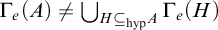 $\Gamma _e(A)\ne \bigcup _{H\subseteq _{\mathrm {hyp}} A} \Gamma _e(H)$
. For example, if A is the graph of a non-hyperarithmetic function and
$\Gamma _e(A)\ne \bigcup _{H\subseteq _{\mathrm {hyp}} A} \Gamma _e(H)$
. For example, if A is the graph of a non-hyperarithmetic function and
 $\Gamma _e$
is such that
$\Gamma _e$
is such that
 $0\in \Gamma _e(B)$
if and only if B contains the graph of some function. None of the hyperarithmetic subsets of A will contain a function, but A does contain a function, so
$0\in \Gamma _e(B)$
if and only if B contains the graph of some function. None of the hyperarithmetic subsets of A will contain a function, but A does contain a function, so
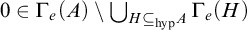 $0\in \Gamma _e(A)\setminus \bigcup _{H\subseteq _{\mathrm {hyp}} A} \Gamma _e(H)$
.
$0\in \Gamma _e(A)\setminus \bigcup _{H\subseteq _{\mathrm {hyp}} A} \Gamma _e(H)$
.
The reason we did not have this problem when adapting the Gutteridge operator was because of the special way that it was constructed. First, it is important to note that for
 $\Pi ^1_1$
sets A we do have
$\Pi ^1_1$
sets A we do have
 $\Gamma _e(A)= \bigcup _{H\subseteq _{\mathrm {hyp}} A} \Gamma _e(H)$
by Claim 4.1.1. This property also holds for sets X of the form
$\Gamma _e(A)= \bigcup _{H\subseteq _{\mathrm {hyp}} A} \Gamma _e(H)$
by Claim 4.1.1. This property also holds for sets X of the form
 $X=\Lambda (A)$
. To see this fix some
$X=\Lambda (A)$
. To see this fix some
 $\Gamma _e$
. For
$\Gamma _e$
. For
 $n\ge e$
we have
$n\ge e$
we have
 $n\in \Gamma _e(X) \iff n\in \Gamma _e(\Lambda (A\restriction n))$
. Here
$n\in \Gamma _e(X) \iff n\in \Gamma _e(\Lambda (A\restriction n))$
. Here
 $\Lambda (A\restriction n)$
is a
$\Lambda (A\restriction n)$
is a
 $\Pi ^1_1$
set, if
$\Pi ^1_1$
set, if
 $n\in \Gamma _e(X)$
then there is some hyperarithmetic
$n\in \Gamma _e(X)$
then there is some hyperarithmetic
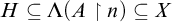 $H\subseteq \Lambda (A\restriction n)\subseteq X$
with
$H\subseteq \Lambda (A\restriction n)\subseteq X$
with
 $n\in \Gamma _e(H)$
. The result for
$n\in \Gamma _e(H)$
. The result for
 $n<e$
comes from some coding of indices of reductions.
$n<e$
comes from some coding of indices of reductions.
We will make use of this idea in the proof of the following.
Theorem 4.2. If A is not
 $\Pi ^1_1$
and
$\Pi ^1_1$
and
 $\Lambda (A)$
is
$\Lambda (A)$
is
 $\Pi ^1_1$
then there are
$\Pi ^1_1$
then there are
 $X<_{he} A$
such that
$X<_{he} A$
such that
 $X>_{he} \mathbf {0}$
.
$X>_{he} \mathbf {0}$
.
Proof. Let
 $(A_s)_{s<{\omega _1^{{CK}}}}$
be an
$(A_s)_{s<{\omega _1^{{CK}}}}$
be an
 $L_{\omega _1^{{CK}}}$
-computable approximation to A. We know that there must be one since
$L_{\omega _1^{{CK}}}$
-computable approximation to A. We know that there must be one since
 $\Lambda (A)$
is
$\Lambda (A)$
is
 $\Pi ^1_1$
. We will build an
$\Pi ^1_1$
. We will build an
 $L_{\omega _1^{{CK}}}$
-c.e. operator
$L_{\omega _1^{{CK}}}$
-c.e. operator
 $\Psi $
, and define
$\Psi $
, and define
 $X=\Psi (A)$
. There are two types of requirements we need to satisfy
$X=\Psi (A)$
. There are two types of requirements we need to satisfy
 $$ \begin{align*}\mathcal{A}_e: X\ne V_e \text{ where } V_e \text{ is the } e\text{ th } \Pi^1_1 \text{ set}\end{align*} $$
that will ensure that
 $\mathbf {0}<_{he} X$
, and
$\mathbf {0}<_{he} X$
, and
 $$ \begin{align*}\mathcal{B}_e: \Gamma_e(X)\ne A\end{align*} $$
that will ensure that
 $A\nleq _{he} X$
. The ordering of requirements is
$A\nleq _{he} X$
. The ordering of requirements is
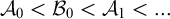 $\mathcal {A}_0<\mathcal {B}_0<\mathcal {A}_1<\dots $
. We will build
$\mathcal {A}_0<\mathcal {B}_0<\mathcal {A}_1<\dots $
. We will build
 $\Psi $
and X in
$\Psi $
and X in
 ${\omega _1^{{CK}}}$
many stages. We will want to be able to add infinitely much to columns of X so we will build X as a subset of
${\omega _1^{{CK}}}$
many stages. We will want to be able to add infinitely much to columns of X so we will build X as a subset of
 ${\omega _1^{{CK}}}^2$
. By fixing an
${\omega _1^{{CK}}}^2$
. By fixing an
 $L_{\omega _1^{{CK}}}$
-computable injection from
$L_{\omega _1^{{CK}}}$
-computable injection from
 ${\omega _1^{{CK}}}$
to
${\omega _1^{{CK}}}$
to
 $\omega $
(for instance the well founded part of a Harrison order) we can turn X into a subset of
$\omega $
(for instance the well founded part of a Harrison order) we can turn X into a subset of
 $\omega $
.
$\omega $
.
We will use an infinite injury construction here, putting the requirements on a tree of strategies. The outcome of node
 $\sigma $
on the tree will be a set
$\sigma $
on the tree will be a set
 $\hat {A}\in L_{\omega _1^{{CK}}}$
that represents the strategy
$\hat {A}\in L_{\omega _1^{{CK}}}$
that represents the strategy
 $\sigma $
’s guess at A at this stage of the construction. Strategies
$\sigma $
’s guess at A at this stage of the construction. Strategies ![]() and below will only add axioms of the form
and below will only add axioms of the form
 $(n, H)$
to
$(n, H)$
to
 $\Psi $
for sets
$\Psi $
for sets
 $H\supseteq \hat {A}$
. This way their work will not interfere with strategies who think
$H\supseteq \hat {A}$
. This way their work will not interfere with strategies who think
 $\hat {A}\nsubseteq A$
. Each strategy
$\hat {A}\nsubseteq A$
. Each strategy
 $\sigma $
can put up a restriction
$\sigma $
can put up a restriction
 $u<{\omega _1^{{CK}}}$
and require that strategies to the right of them on the tree only put things in columns
$u<{\omega _1^{{CK}}}$
and require that strategies to the right of them on the tree only put things in columns
 $\ge u$
of X. For
$\ge u$
of X. For
 $\sigma $
we consider its restriction u to be the
$\sigma $
we consider its restriction u to be the
 $\sup $
of all the restrictions put up by nodes to the left of or above
$\sup $
of all the restrictions put up by nodes to the left of or above
 $\sigma $
. The ordering of outcomes is
$\sigma $
. The ordering of outcomes is
 $\hat {A}<\hat {B}$
if
$\hat {A}<\hat {B}$
if
 $\hat {A}\supseteq \hat {B}$
. This is only a partial order on sets, but we will see in the construction that we only use a limited collection of outcomes for each strategy, and this collection will be linearly ordered. We will argue that the leftmost path visited cofinally often is correct in its guesses about A and along this path all requirements are met. When a strategy has outcome
$\hat {A}\supseteq \hat {B}$
. This is only a partial order on sets, but we will see in the construction that we only use a limited collection of outcomes for each strategy, and this collection will be linearly ordered. We will argue that the leftmost path visited cofinally often is correct in its guesses about A and along this path all requirements are met. When a strategy has outcome
 $\hat {A}$
to the left of a previous outcome
$\hat {A}$
to the left of a previous outcome
 $\hat {B}$
, it adds
$\hat {B}$
, it adds
 $(n,\hat {A})$
to
$(n,\hat {A})$
to
 $\Psi $
for all n added by strategies below
$\Psi $
for all n added by strategies below
 $\hat {B}$
to ensure that axioms added by strategies below
$\hat {B}$
to ensure that axioms added by strategies below
 $\hat {B}$
cannot interfere with the strategies below
$\hat {B}$
cannot interfere with the strategies below
 $\hat {A}$
.
$\hat {A}$
.
Strategies. The strategy for a node
 $\sigma $
of requirement
$\sigma $
of requirement
 $\mathcal {B}_e$
is to find a witness m where
$\mathcal {B}_e$
is to find a witness m where
 $m\in A\setminus \Gamma _{e}(X)$
. When this strategy is initialized at some stage s it is given outcome
$m\in A\setminus \Gamma _{e}(X)$
. When this strategy is initialized at some stage s it is given outcome
 $\hat {A}$
from its parent node and restriction u, the
$\hat {A}$
from its parent node and restriction u, the
 $\sup $
of the restrictions put up by nodes to the left of
$\sup $
of the restrictions put up by nodes to the left of
 $\sigma $
.
$\sigma $
.
 $\sigma $
has one variable
$\sigma $
has one variable
 $m_s$
that it keeps track of. When initialized, we start with
$m_s$
that it keeps track of. When initialized, we start with
 $m_{s+1}=0$
. At a limit stage s, we define
$m_{s+1}=0$
. At a limit stage s, we define
 $m_s=\liminf _{t<s}m_t$
if that exists, otherwise
$m_s=\liminf _{t<s}m_t$
if that exists, otherwise
 $m_s=0$
. We also have
$m_s=0$
. We also have
 $X_s=\Psi _s(\hat {A})$
which is
$X_s=\Psi _s(\hat {A})$
which is
 $\sigma $
’s guess at X at stage s. In the verification, we will prove that
$\sigma $
’s guess at X at stage s. In the verification, we will prove that
 $X_s$
eventually agrees with X on the first u many columns, that
$X_s$
eventually agrees with X on the first u many columns, that
 $m=\lim _{s<{\omega _1^{{CK}}}}m_s$
exists, and that
$m=\lim _{s<{\omega _1^{{CK}}}}m_s$
exists, and that
 $A(m)\ne \Gamma _{e}(X)(m)$
.
$A(m)\ne \Gamma _{e}(X)(m)$
.
Given
 $m_s$
and
$m_s$
and
 $X_s$
at stage s, the strategy asks if
$X_s$
at stage s, the strategy asks if
 $m_s\notin \Gamma _{e,s}(X_s)$
and there is some
$m_s\notin \Gamma _{e,s}(X_s)$
and there is some
 $H\in L_s$
such that
$H\in L_s$
such that
 $H\subseteq ({\omega _1^{{CK}}}\setminus u)\times {\omega _1^{{CK}}}$
and
$H\subseteq ({\omega _1^{{CK}}}\setminus u)\times {\omega _1^{{CK}}}$
and
 $m_s\in \Gamma _{e,s}(X_s\cup H)$
. If yes, then we put
$m_s\in \Gamma _{e,s}(X_s\cup H)$
. If yes, then we put
 $m_s\in X$
: we add axioms
$m_s\in X$
: we add axioms
 $(\langle \alpha , \beta \rangle , \hat {A})$
to
$(\langle \alpha , \beta \rangle , \hat {A})$
to
 $\Psi _{s+1}$
for each
$\Psi _{s+1}$
for each
 $\langle \alpha , \beta \rangle \in X_s\cup H$
with
$\langle \alpha , \beta \rangle \in X_s\cup H$
with
 $\alpha \ge u$
. This will injure all lower priority
$\alpha \ge u$
. This will injure all lower priority
 $\mathcal {A}$
requirements. If no and
$\mathcal {A}$
requirements. If no and
 $m_s\notin (A_s\cup \hat {A}) \triangle \Gamma _{e,s}(X_s)$
, then we need to pick a new witness: set
$m_s\notin (A_s\cup \hat {A}) \triangle \Gamma _{e,s}(X_s)$
, then we need to pick a new witness: set
 $m_{s+1}$
to be the least m in
$m_{s+1}$
to be the least m in
 $(A_s\cup \hat {A}) \triangle \Gamma _{e,s}(X_s)$
. Otherwise
$(A_s\cup \hat {A}) \triangle \Gamma _{e,s}(X_s)$
. Otherwise
 $m_{s+1}=m_s$
. No matter what, the outcome of
$m_{s+1}=m_s$
. No matter what, the outcome of
 $\sigma $
is always
$\sigma $
is always
 $\hat {A}$
, and
$\hat {A}$
, and
 $\sigma $
does not put up any restriction.
$\sigma $
does not put up any restriction.
The strategy for a node
 $\tau $
of requirement
$\tau $
of requirement
 $\mathcal {A}_e$
is as follows. We will try to build an
$\mathcal {A}_e$
is as follows. We will try to build an
 $L_{\omega _1^{{CK}}}$
-c.e. approximation
$L_{\omega _1^{{CK}}}$
-c.e. approximation
 $(P_s)_{s}$
to A by encoding parts of A into column u of X. The approximation to A will eventually fail, as A is not
$(P_s)_{s}$
to A by encoding parts of A into column u of X. The approximation to A will eventually fail, as A is not
 $L_{\omega _1^{{CK}}}$
-c.e, and we will use this point of difference to ensure that
$L_{\omega _1^{{CK}}}$
-c.e, and we will use this point of difference to ensure that
 $X\ne V_e$
. To this end we will build a sequence of coding points
$X\ne V_e$
. To this end we will build a sequence of coding points
 $(n_\beta ,m_\beta )_{\beta <\alpha _s}$
. The only changes we will make to this sequence are to add a new element to the sequence or remove the last element (if there is one). So at limit stages s we can have
$(n_\beta ,m_\beta )_{\beta <\alpha _s}$
. The only changes we will make to this sequence are to add a new element to the sequence or remove the last element (if there is one). So at limit stages s we can have
 $\alpha _s=\liminf _{t<s}\alpha _t$
and that will ensure that all the coding points are well defined at stage s. The idea with the coding points is that for all but the top one we have ensured that
$\alpha _s=\liminf _{t<s}\alpha _t$
and that will ensure that all the coding points are well defined at stage s. The idea with the coding points is that for all but the top one we have ensured that
 $\langle u, n_\beta \rangle \in V_e$
and that
$\langle u, n_\beta \rangle \in V_e$
and that
 $\langle u, n_\beta \rangle \in X$
only if
$\langle u, n_\beta \rangle \in X$
only if
 $m_\beta \in A$
. Our approximation
$m_\beta \in A$
. Our approximation
 $P_s$
will be
$P_s$
will be
 $\hat {A} \cup \{m_\beta : \langle u, n_\beta \rangle \in V_{e,s}\}$
. Since
$\hat {A} \cup \{m_\beta : \langle u, n_\beta \rangle \in V_{e,s}\}$
. Since
 $V_{e,s}$
is increasing,
$V_{e,s}$
is increasing,
 $P_s$
is increasing as long as we do not remove coding points
$P_s$
is increasing as long as we do not remove coding points
 $(n_\beta ,m_\beta )$
after putting
$(n_\beta ,m_\beta )$
after putting
 $m_\beta \in P$
.
$m_\beta \in P$
.
We are trying to make
 $X\neq V_e$
, so when we notice
$X\neq V_e$
, so when we notice
 $m_\beta \notin A_s$
it appears that we have succeeded and do not need to do anything. The problem with this is that once we have
$m_\beta \notin A_s$
it appears that we have succeeded and do not need to do anything. The problem with this is that once we have
 $\alpha _s>\omega $
there are infinitely many
$\alpha _s>\omega $
there are infinitely many
 $m_\beta $
so we may see
$m_\beta $
so we may see
 $m_\beta \notin A_t$
for a different
$m_\beta \notin A_t$
for a different
 $\beta $
at each stage
$\beta $
at each stage
 $t>s$
but have
$t>s$
but have
 $m_\beta \in A$
for all
$m_\beta \in A$
for all
 $\beta <\alpha _s$
. We could avoid this problem if we knew that
$\beta <\alpha _s$
. We could avoid this problem if we knew that
 $A_s$
stabilized on hyperarithmetic sets, but we only know that it stabilizes on finite sets. This is enough for us, but we will have to keep track of the
$A_s$
stabilized on hyperarithmetic sets, but we only know that it stabilizes on finite sets. This is enough for us, but we will have to keep track of the
 $\beta $
where
$\beta $
where
 $m_\beta \notin A_s$
, and sometimes our outcome will need to include numbers that are not in
$m_\beta \notin A_s$
, and sometimes our outcome will need to include numbers that are not in
 $A_s$
.
$A_s$
.
To this end,
 $\tau $
will keep track of a finite sequence of victories
$\tau $
will keep track of a finite sequence of victories
 $\hat {\beta }_s=\beta _0>\beta _1>\dots >\beta _{k-1}$
with the property that
$\hat {\beta }_s=\beta _0>\beta _1>\dots >\beta _{k-1}$
with the property that
 $m_{\beta _0}<\dots <m_{\beta _{k-1}}$
are numbers we thought were out of A at the previous stage. When
$m_{\beta _0}<\dots <m_{\beta _{k-1}}$
are numbers we thought were out of A at the previous stage. When
 $\tau $
is initialized we start with
$\tau $
is initialized we start with
 $\hat {\beta }=\emptyset $
and at limit stages s we define
$\hat {\beta }=\emptyset $
and at limit stages s we define
 $\hat {\beta }_s$
to be the longest sequence
$\hat {\beta }_s$
to be the longest sequence
 $\hat {\beta }$
such that
$\hat {\beta }$
such that
 $\hat {\beta }_i=\lim _{t<s}\hat {\beta }_{t,i}$
. At a stage s the requirement updates the victories as the first step. We consider
$\hat {\beta }_i=\lim _{t<s}\hat {\beta }_{t,i}$
. At a stage s the requirement updates the victories as the first step. We consider
 $\beta $
such that
$\beta $
such that
 $m_\beta $
is the smallest
$m_\beta $
is the smallest
 $m\in \overline { A_s}$
with the property for all
$m\in \overline { A_s}$
with the property for all
 $i<k$
,
$i<k$
,
 $m_{\beta _i}\leq m\implies \beta _i>\beta $
. If there is such a
$m_{\beta _i}\leq m\implies \beta _i>\beta $
. If there is such a
 $\beta $
then we add it to our sequence of victories for
$\beta $
then we add it to our sequence of victories for
 $\hat {\beta }_{s+1}$
and remove all victories
$\hat {\beta }_{s+1}$
and remove all victories
 $\beta _i<\beta $
. Next we remove invalid victories: if there is any
$\beta _i<\beta $
. Next we remove invalid victories: if there is any
 $i<k$
such that
$i<k$
such that
 $m_{\beta _i}\in A_s$
then we remove that victory and all victories for
$m_{\beta _i}\in A_s$
then we remove that victory and all victories for
 $j\ge i$
. The reason we also remove larger victories is to deal with the fact that
$j\ge i$
. The reason we also remove larger victories is to deal with the fact that
 $A_s$
only stabilizes on finite sets. In the verification we will prove that an initial segment of
$A_s$
only stabilizes on finite sets. In the verification we will prove that an initial segment of
 $\hat {\beta }_s$
stabilizes, and to ensure that initial segment is
$\hat {\beta }_s$
stabilizes, and to ensure that initial segment is
 $\beta _s$
cofinally often, we need to remove smaller
$\beta _s$
cofinally often, we need to remove smaller
 $\beta _i$
whenever we see a change.
$\beta _i$
whenever we see a change.
If the sequence of victories has become empty, then we think
 $P_s\subseteq A$
so we need to consider adding a coding point. If
$P_s\subseteq A$
so we need to consider adding a coding point. If
 $\alpha _s$
is a successor, then we consider the highest coding point
$\alpha _s$
is a successor, then we consider the highest coding point
 $(n,m)$
. If
$(n,m)$
. If
 $\langle u,n\rangle \in X\setminus V_e$
then we can satisfy the
$\langle u,n\rangle \in X\setminus V_e$
then we can satisfy the
 $\mathcal {A}_e$
without any victories. So if
$\mathcal {A}_e$
without any victories. So if
 $\langle u,n\rangle \notin V_{e,s}$
and
$\langle u,n\rangle \notin V_{e,s}$
and
 $m\notin A_s$
, then we add the axiom
$m\notin A_s$
, then we add the axiom
 $(\langle u,n\rangle , P_s)$
to
$(\langle u,n\rangle , P_s)$
to
 $\Psi _{s+1}$
to keep
$\Psi _{s+1}$
to keep
 $\langle u,n\rangle \in X$
. This will, however, invalidate the coding point, meaning we will have to remove it and try again if we ever see
$\langle u,n\rangle \in X$
. This will, however, invalidate the coding point, meaning we will have to remove it and try again if we ever see
 $\langle u,n\rangle $
enter
$\langle u,n\rangle $
enter
 $V_e$
. If
$V_e$
. If
 $\langle u,n\rangle \in V_e$
then it is time to add a new coding point. If
$\langle u,n\rangle \in V_e$
then it is time to add a new coding point. If
 $(n,m)$
has been invalidated, then we remove it from the sequence of coding points first. If
$(n,m)$
has been invalidated, then we remove it from the sequence of coding points first. If
 $(n,m)$
has not been invalidated then we add m to
$(n,m)$
has not been invalidated then we add m to
 $P_{s+1}$
. To pick a new coding point we choose
$P_{s+1}$
. To pick a new coding point we choose
 $n_{\alpha _s}$
to be the least unused number in column u and
$n_{\alpha _s}$
to be the least unused number in column u and
 $m_{\alpha _s}$
to be the least member of
$m_{\alpha _s}$
to be the least member of
 $A_s\setminus P_s$
if there is one. We then add the axiom
$A_s\setminus P_s$
if there is one. We then add the axiom
 $(\langle u,n_{\alpha _s}\rangle , P_s\cup \{m_{\alpha _s}\})$
to
$(\langle u,n_{\alpha _s}\rangle , P_s\cup \{m_{\alpha _s}\})$
to
 $\Psi _{s+1}$
. If
$\Psi _{s+1}$
. If
 $A_s\subseteq P_s$
then we cannot add a new coding point yet.
$A_s\subseteq P_s$
then we cannot add a new coding point yet.
If there are no victories and
 $\alpha _s$
is a limit or
$\alpha _s$
is a limit or
 $0$
, then we proceed to add a new coding point as above.
$0$
, then we proceed to add a new coding point as above.
Finally we come to defining the outcome and restriction of
 $\tau $
. We always impose restriction
$\tau $
. We always impose restriction
 $u+1$
on lower priority requirements so they cannot interfere with our coding points in column u. To define the outcome, we use the sequence of victories. If there are no victories this means we have outcome
$u+1$
on lower priority requirements so they cannot interfere with our coding points in column u. To define the outcome, we use the sequence of victories. If there are no victories this means we have outcome
 $P_s$
since it looks like
$P_s$
since it looks like
 $P_s\subseteq A$
. If there are victories, then we consider the least victory
$P_s\subseteq A$
. If there are victories, then we consider the least victory
 $\beta _{k-1}$
. Since it looks like
$\beta _{k-1}$
. Since it looks like
 $m_{\beta _{k-1}}\notin A$
but
$m_{\beta _{k-1}}\notin A$
but
 $m_\beta \in A$
for all
$m_\beta \in A$
for all
 $\beta <\beta _{k-1}$
we give outcome
$\beta <\beta _{k-1}$
we give outcome
 $\hat {A}\cup \{m_\beta : \beta <\beta _{k-1}\}$
. Note that, as promised above, the collection of outcomes is linearly ordered.
$\hat {A}\cup \{m_\beta : \beta <\beta _{k-1}\}$
. Note that, as promised above, the collection of outcomes is linearly ordered.
Verification. We will use induction to argue that for each node
 $\sigma $
on the true path, the following hold:
$\sigma $
on the true path, the following hold:
-
1. There is a left most outcome
$\hat {A}$
that is visited cofinally often. -
2.
$\hat {A}\subseteq A$
. -
3. For all
$\hat {B}<\hat {A}$
that were outcomes of
$\sigma $
we have
$\hat {B}\nsubseteq A$
. -
4.
$\Psi (\hat {A})^{[u]}=\Psi (A)^{[u]}$
. -
5.
$\sigma $
stops adding axioms to
$\Psi $
after some stage. -
6. The requirement for
$\sigma $
is satisfied.


We start with the case where
 $\sigma $
is a strategy for a
$\sigma $
is a strategy for a
 $\mathcal {B}_e$
requirement. Let s be a stage after which no node to the left of
$\mathcal {B}_e$
requirement. Let s be a stage after which no node to the left of
 $\sigma $
is visited and no node above
$\sigma $
is visited and no node above
 $\sigma $
adds axioms to
$\sigma $
adds axioms to
 $\Psi $
. In this case
$\Psi $
. In this case
 $\sigma $
only has one outcome
$\sigma $
only has one outcome
 $\hat {A}$
, and since it only adds axioms using
$\hat {A}$
, and since it only adds axioms using
 $\hat {A}$
, 1. through 4. hold. So we just need to check that the requirement was met and stops adding axioms. Consider the set
$\hat {A}$
, 1. through 4. hold. So we just need to check that the requirement was met and stops adding axioms. Consider the set
 $W=\bigcup _{s<{\omega _1^{{CK}}}} \Gamma _{e,s}(X_s)=\lim _{s<{\omega _1^{{CK}}}}\Gamma _{e,s}(X_s)$
. Since W is
$W=\bigcup _{s<{\omega _1^{{CK}}}} \Gamma _{e,s}(X_s)=\lim _{s<{\omega _1^{{CK}}}}\Gamma _{e,s}(X_s)$
. Since W is
 $L_{\omega _1^{{CK}}}$
-c.e. there is some least
$L_{\omega _1^{{CK}}}$
-c.e. there is some least
 $m\in W\triangle A$
. So we have that
$m\in W\triangle A$
. So we have that
 $m=\lim _{s<{\omega _1^{{CK}}}} m_s$
, and once this limit settles down
$m=\lim _{s<{\omega _1^{{CK}}}} m_s$
, and once this limit settles down
 $\sigma $
puts axioms into
$\sigma $
puts axioms into
 $\Psi $
at most once more, so 5. is satisfied.
$\Psi $
at most once more, so 5. is satisfied.
Now to show the requirement is met. We have two cases. Case 1: Suppose that
 $m\in W$
. Then
$m\in W$
. Then
 $m\notin A$
and
$m\notin A$
and
 $m\in \Gamma _e(X)$
since
$m\in \Gamma _e(X)$
since
 $X_s\subseteq \Psi _s(\hat {A})\subseteq \Psi (A)=X$
, so the requirement is satisfied.
$X_s\subseteq \Psi _s(\hat {A})\subseteq \Psi (A)=X$
, so the requirement is satisfied.
Case 2: Suppose that
 $m\in A$
. Then consider the set
$m\in A$
. Then consider the set
 $X^*= \Psi (\hat {A}) \cup \{n: \exists H, \tau \prec \sigma [\tau \text { put }(n,H)\in \Psi ]\}$
. Since any number put into X by a strategy to the right of
$X^*= \Psi (\hat {A}) \cup \{n: \exists H, \tau \prec \sigma [\tau \text { put }(n,H)\in \Psi ]\}$
. Since any number put into X by a strategy to the right of
 $\sigma $
is put into X with a subset of
$\sigma $
is put into X with a subset of
 $\hat {A}$
when we next visit
$\hat {A}$
when we next visit
 $\sigma $
, and because requirements to the left of
$\sigma $
, and because requirements to the left of
 $\sigma $
only add axioms
$\sigma $
only add axioms
 $(n,H)$
for
$(n,H)$
for
 $H\nsubseteq A$
by 3., we have that
$H\nsubseteq A$
by 3., we have that
 $X\subseteq X^*$
and
$X\subseteq X^*$
and
 $X^{[v]}=X^{*[v]}$
for all
$X^{[v]}=X^{*[v]}$
for all
 $v<u$
. It is clear that
$v<u$
. It is clear that
 $X^*$
is
$X^*$
is
 $L_{\omega _1^{{CK}}}$
-c.e. so if
$L_{\omega _1^{{CK}}}$
-c.e. so if
 $m\in \Gamma _e(X^*)$
then by Claim 4.1.1 there is
$m\in \Gamma _e(X^*)$
then by Claim 4.1.1 there is
 $t<{\omega _1^{{CK}}}$
and hyperarithmetic
$t<{\omega _1^{{CK}}}$
and hyperarithmetic
 $H\subseteq X^*$
such that
$H\subseteq X^*$
such that
 $m\in \Gamma _{e,t}(H)$
. Since X and
$m\in \Gamma _{e,t}(H)$
. Since X and
 $X^*$
agree on the first u many columns we have that
$X^*$
agree on the first u many columns we have that
 $m\in W$
as
$m\in W$
as
 $\sigma $
will have acted at some stage
$\sigma $
will have acted at some stage
 $\ge t$
to ensure this. But
$\ge t$
to ensure this. But
 $m\in A$
, a contradiction, so
$m\in A$
, a contradiction, so
 $m\notin \Gamma _e(X^*)\supseteq \Gamma _e(X)$
. So the requirement is satisfied.
$m\notin \Gamma _e(X^*)\supseteq \Gamma _e(X)$
. So the requirement is satisfied.
Now we consider the case where
 $\sigma $
is a strategy for an
$\sigma $
is a strategy for an
 $\mathcal {A}_e$
requirement. First we will argue that we stop adding coding locations after some stage. Consider the set
$\mathcal {A}_e$
requirement. First we will argue that we stop adding coding locations after some stage. Consider the set
 $P=\bigcup _s P_s$
. This is an
$P=\bigcup _s P_s$
. This is an
 $L_{\omega _1^{{CK}}}$
-c.e. set, so there is some least
$L_{\omega _1^{{CK}}}$
-c.e. set, so there is some least
 $m\in P\triangle A$
. Consider some stage s such that
$m\in P\triangle A$
. Consider some stage s such that
 $A{\restriction } m+1 = A_t{\restriction } m+1=P_s{\restriction } m+1 \triangle \{m\}$
for all
$A{\restriction } m+1 = A_t{\restriction } m+1=P_s{\restriction } m+1 \triangle \{m\}$
for all
 $t>s$
. If
$t>s$
. If
 $m\in P$
then after stage s we will always have
$m\in P$
then after stage s we will always have
 $m=m_{\beta _0}$
as the first victory, so
$m=m_{\beta _0}$
as the first victory, so
 $\sigma $
will stop growing P and will not add any more coding locations. If
$\sigma $
will stop growing P and will not add any more coding locations. If
 $m\notin P$
then after stage s whenever we chose a new coding location
$m\notin P$
then after stage s whenever we chose a new coding location
 $(n',m')$
we will have
$(n',m')$
we will have
 $m'=m$
. Since m never leaves
$m'=m$
. Since m never leaves
 $A_t$
this location will never be invalidated, so, since
$A_t$
this location will never be invalidated, so, since
 $m\notin P$
, it must be that
$m\notin P$
, it must be that
 $\langle u, n'\rangle \notin V_e$
so we stop adding coding locations. In either case 5. is satisfied.
$\langle u, n'\rangle \notin V_e$
so we stop adding coding locations. In either case 5. is satisfied.
Next we argue that the sequence of victories stabilizes on an initial segment. If
 $P\subseteq A$
then this initial segment will be the empty set. Otherwise, observe that
$P\subseteq A$
then this initial segment will be the empty set. Otherwise, observe that
 $P_s=\{m_\beta : \beta <\alpha _s\}$
(with the last element excluded if it has not been added). Consider the sequence
$P_s=\{m_\beta : \beta <\alpha _s\}$
(with the last element excluded if it has not been added). Consider the sequence
 $(\beta _i)_{i<k}$
defined by taking
$(\beta _i)_{i<k}$
defined by taking
 $\beta _i$
is the least
$\beta _i$
is the least
 $\beta $
such that
$\beta $
such that
 $m_\beta $
is the least element of
$m_\beta $
is the least element of
 $\{m_\beta : \beta <\beta _{i-1}\} \setminus A$
if this set is nonempty. Since
$\{m_\beta : \beta <\beta _{i-1}\} \setminus A$
if this set is nonempty. Since
 $\alpha _s$
is well founded this sequence must be finite and have some length k. Consider a stage s after which
$\alpha _s$
is well founded this sequence must be finite and have some length k. Consider a stage s after which
 $A_t{\restriction } m_{\beta _{k-1}}+1$
and
$A_t{\restriction } m_{\beta _{k-1}}+1$
and
 $P_t$
have stabilized. At all stages
$P_t$
have stabilized. At all stages
 $t>s$
where
$t>s$
where
 $\sigma $
is visited we must have
$\sigma $
is visited we must have
 $\beta _0>\dots >\beta _k$
as a proper initial segment of the sequence of victories as these are all true victories and no other victories could be added for
$\beta _0>\dots >\beta _k$
as a proper initial segment of the sequence of victories as these are all true victories and no other victories could be added for
 $m_\beta <m_{\beta _{k-1}}$
after stage s. So after stage s the outcome of
$m_\beta <m_{\beta _{k-1}}$
after stage s. So after stage s the outcome of
 $\sigma $
will always be a subset of
$\sigma $
will always be a subset of
 $\hat {A}:=\hat {B} \cup \{m_\beta : \beta <\beta _{k-1}\}$
where
$\hat {A}:=\hat {B} \cup \{m_\beta : \beta <\beta _{k-1}\}$
where
 $\hat {B}$
was the outcome of the parent of
$\hat {B}$
was the outcome of the parent of
 $\sigma $
. We now claim that
$\sigma $
. We now claim that
 $\hat {A}$
will satisfy 1. through 3.
$\hat {A}$
will satisfy 1. through 3.
If the outcome is ever
 $\hat {C}<\hat {A}$
then it must be that
$\hat {C}<\hat {A}$
then it must be that
 $m_{\beta _{k-1}}\in \hat {C}$
so 3. is satisfied and after stage s we never have any outcome left of
$m_{\beta _{k-1}}\in \hat {C}$
so 3. is satisfied and after stage s we never have any outcome left of
 $\hat {A}$
. Since we could not extend our sequence
$\hat {A}$
. Since we could not extend our sequence
 $(\beta +i)_{i<k}$
it must be that
$(\beta +i)_{i<k}$
it must be that
 $\hat {A}\subseteq A$
so 2. is satisfied. This also means that any victory
$\hat {A}\subseteq A$
so 2. is satisfied. This also means that any victory
 $\beta $
added to the end of our sequence of victories must have
$\beta $
added to the end of our sequence of victories must have
 $m_\beta \in A$
. This means that
$m_\beta \in A$
. This means that
 $\beta $
will eventually be removed from our sequence of victories when we see
$\beta $
will eventually be removed from our sequence of victories when we see
 $m_\beta \in A_t$
for some t. We remove a victory, we also remove all victories for
$m_\beta \in A_t$
for some t. We remove a victory, we also remove all victories for
 $m>m_\beta $
, so there will be cofinally many stages where the sequence of victories is just
$m>m_\beta $
, so there will be cofinally many stages where the sequence of victories is just
 $(\beta _i)_{i<k}$
. Hence the outcome of
$(\beta _i)_{i<k}$
. Hence the outcome of
 $\sigma $
will cofinally often be
$\sigma $
will cofinally often be
 $\hat {A}$
, satisfying 1. To see 4. recall that when coding location
$\hat {A}$
, satisfying 1. To see 4. recall that when coding location
 $(n,m)$
was added at stage t we used
$(n,m)$
was added at stage t we used
 $P_t\cup \{m\}$
to put it in X. So if it was added before the coding location
$P_t\cup \{m\}$
to put it in X. So if it was added before the coding location
 $(n_{\beta _{k-1}},m_{\beta _{k-1}})$
was added then
$(n_{\beta _{k-1}},m_{\beta _{k-1}})$
was added then
 $\langle u, n\rangle \in \Psi _e(\hat {A})$
, and if it was added after, then
$\langle u, n\rangle \in \Psi _e(\hat {A})$
, and if it was added after, then
 $\langle u, n\rangle \notin \Psi (A)$
.
$\langle u, n\rangle \notin \Psi (A)$
.
To see that the requirement for
 $\sigma $
is satisfied, we need to look at two cases. First, if the sequence of victories was empty this meant that
$\sigma $
is satisfied, we need to look at two cases. First, if the sequence of victories was empty this meant that
 $P\subseteq A$
and we stopped adding coding locations because the top location
$P\subseteq A$
and we stopped adding coding locations because the top location
 $(n,m)$
had
$(n,m)$
had
 $\langle u,n\rangle \notin V_e$
. If this location was never invalidated then,
$\langle u,n\rangle \notin V_e$
. If this location was never invalidated then,
 $m\in A$
and
$m\in A$
and
 $\langle u,n\rangle \in \Psi (A)$
. If it was invalidated, then we added the axiom
$\langle u,n\rangle \in \Psi (A)$
. If it was invalidated, then we added the axiom
 $(\langle u,n\rangle , P)$
to
$(\langle u,n\rangle , P)$
to
 $\Psi $
so
$\Psi $
so
 $\langle u,n\rangle \in \Psi (A)$
. Second, if the sequence of victories was not empty then
$\langle u,n\rangle \in \Psi (A)$
. Second, if the sequence of victories was not empty then
 $m_{\beta _0}\notin A$
, so
$m_{\beta _0}\notin A$
, so
 $\langle u,n_{\beta _0}\rangle \notin \Psi (A)$
but
$\langle u,n_{\beta _0}\rangle \notin \Psi (A)$
but
 $m_{\beta _0}\in P$
so
$m_{\beta _0}\in P$
so
 $\langle u, n_{\beta _0}\rangle \in V_e$
.
$\langle u, n_{\beta _0}\rangle \in V_e$
.
This completes the induction. Note that condition 1. ensures that there is a true path. Since each requirement on the true path is satisfied we have that X is not
 $L_{\omega _1^{{CK}}}$
-c.e. and
$L_{\omega _1^{{CK}}}$
-c.e. and
 $A\nleq _{he} X$
. The fact that
$A\nleq _{he} X$
. The fact that
 $X\le _{he} A$
follows from Proposition 5.4, which is proved in the next section. In Section 5 we explore other other reducibilities including a reducibility defined in terms of
$X\le _{he} A$
follows from Proposition 5.4, which is proved in the next section. In Section 5 we explore other other reducibilities including a reducibility defined in terms of
 $L_{\omega _1^{{CK}}}$
-c.e. operators like
$L_{\omega _1^{{CK}}}$
-c.e. operators like
 $\Psi $
. Proposition 5.4 states that reductions via
$\Psi $
. Proposition 5.4 states that reductions via
 $L_{\omega _1^{{CK}}}$
-c.e. operators imply hyperenumeration reducibility.
$L_{\omega _1^{{CK}}}$
-c.e. operators imply hyperenumeration reducibility.
5 Other reducibilities
We now look at some other reducibilities that are different from
 $\le _{he}$
but could be considered notions of hyperenumeration reducibility. We show most of these reducibilities
$\le _{he}$
but could be considered notions of hyperenumeration reducibility. We show most of these reducibilities
 $\le _*$
share some of the properties of
$\le _*$
share some of the properties of
 $\le _{he}$
, like extending enumeration reducibility and having
$\le _{he}$
, like extending enumeration reducibility and having
 $A\le _* B\oplus \overline {B}\iff A$
is
$A\le _* B\oplus \overline {B}\iff A$
is
 $\Pi ^1_1$
in B. The first reducibility to consider is the notion of relatively
$\Pi ^1_1$
in B. The first reducibility to consider is the notion of relatively
 $\Pi ^1_1$
.
$\Pi ^1_1$
.
Definition 5.1. We say that A is relatively
 $\Pi ^1_1$
in B,
$\Pi ^1_1$
in B,
 $A\le _{\Pi ^1_1} B$
, if whenever B is
$A\le _{\Pi ^1_1} B$
, if whenever B is
 $\Pi ^1_1$
in X we have that A is
$\Pi ^1_1$
in X we have that A is
 $\Pi ^1_1$
in X.
$\Pi ^1_1$
in X.
We say that A is uniformly relatively
 $\Pi ^1_1$
in B,
$\Pi ^1_1$
in B,
 $A\le _{u\Pi ^1_1} B$
, if there is a computable f such that if
$A\le _{u\Pi ^1_1} B$
, if there is a computable f such that if
 $B= \Gamma _e(X\oplus \overline {X})$
then
$B= \Gamma _e(X\oplus \overline {X})$
then
 $ A= \Gamma _{f(e)}(X\oplus \overline {X})$
We used hyperenumeration operators to define
 $\le _{u\Pi ^1_1}$
, but it could equivalently be defined by saying there is Turing operator that turns hyperenumerations of B into hyperenumerations of A or that there is a computable function that turns
$\le _{u\Pi ^1_1}$
, but it could equivalently be defined by saying there is Turing operator that turns hyperenumerations of B into hyperenumerations of A or that there is a computable function that turns
 $\Pi ^1_1$
formulas for B into
$\Pi ^1_1$
formulas for B into
 $\Pi ^1_1$
formulas for A.
$\Pi ^1_1$
formulas for A.
The fact that composition of hyperenumeration operators is uniform means that
 $A\le _{he}B\implies A\le _{u\Pi ^1_1} B$
and by definition we have
$A\le _{he}B\implies A\le _{u\Pi ^1_1} B$
and by definition we have
 $A\le _{u\Pi ^1_1} B\implies A\le _{\Pi ^1_1}B$
. It is natural to ask if these implications are strict. From Theorem 3.1 we can see that
$A\le _{u\Pi ^1_1} B\implies A\le _{\Pi ^1_1}B$
. It is natural to ask if these implications are strict. From Theorem 3.1 we can see that
 $\le _{he}$
is different from
$\le _{he}$
is different from
 $\le _{\Pi ^1_1}$
because by definition each relatively
$\le _{\Pi ^1_1}$
because by definition each relatively
 $\Pi ^1_1$
degree is uniquely determined by the total degrees above it. A closer look at the proof of Corollary 3.8 shows us that
$\Pi ^1_1$
degree is uniquely determined by the total degrees above it. A closer look at the proof of Corollary 3.8 shows us that
 $\overline {T}\le _{u\Pi ^1_1} T$
for any uniformly e-pointed tree without dead ends, hence
$\overline {T}\le _{u\Pi ^1_1} T$
for any uniformly e-pointed tree without dead ends, hence
 $\le _{he}$
and
$\le _{he}$
and
 $\le _{u\Pi ^1_1}$
are different. The remaining possible separation is an open question.
$\le _{u\Pi ^1_1}$
are different. The remaining possible separation is an open question.
Question 5.2. Are there sets A and B such that
 $A\le _{\Pi ^1_1} B$
and
$A\le _{\Pi ^1_1} B$
and
 $A\not \le _{u\Pi ^1_1} B$
?
$A\not \le _{u\Pi ^1_1} B$
?
A negative answer to the above question could be seen as a proof of Selman’s theorem for
 $\le _{u\Pi ^1_1}$
. One approach to try to answer this question is to see if one can transform Selman’s original proof to this context.
$\le _{u\Pi ^1_1}$
. One approach to try to answer this question is to see if one can transform Selman’s original proof to this context.
On the other hand, we observe that the uniformity of an e-pointed tree T without dead ends is important for the proof of
 $\overline {T}\le _{u\Pi ^1_1} T$
. Perhaps there is a sufficiently generic non-uniformly e-pointed tree T without dead ends such that
$\overline {T}\le _{u\Pi ^1_1} T$
. Perhaps there is a sufficiently generic non-uniformly e-pointed tree T without dead ends such that
 $\overline {T}\not \le _{u\Pi ^1_1} T$
. Such a result would be interesting because it would suggest that there is no notion hyperenumeration operators for relatively
$\overline {T}\not \le _{u\Pi ^1_1} T$
. Such a result would be interesting because it would suggest that there is no notion hyperenumeration operators for relatively
 $\Pi ^1_1$
, i.e., no nice listing of functions on
$\Pi ^1_1$
, i.e., no nice listing of functions on
 $2^\omega $
such that if
$2^\omega $
such that if
 $A\le _{\Pi ^1_1} B$
then there is one of these functions,
$A\le _{\Pi ^1_1} B$
then there is one of these functions,
 $\Gamma $
such that
$\Gamma $
such that
 $A=\Gamma (B)$
.
$A=\Gamma (B)$
.
Another way that may be natural to define hyperenumeration reducibility is by changing the nature of the set W in the usual definition of enumeration reducibility.
Definition 5.3. We say that A is continuously higher enumeration reducible to B,
 $A\le _{che}B$
if there is a
$A\le _{che}B$
if there is a
 $\Pi ^1_1$
set W such that
$\Pi ^1_1$
set W such that
 $n\in A \iff \exists u [\langle n,u\rangle \in W\land D_u\subseteq B]$
.
$n\in A \iff \exists u [\langle n,u\rangle \in W\land D_u\subseteq B]$
.
We say that A is
 ${\omega _1^{{CK}}}$
-enumeration reducible to B,
${\omega _1^{{CK}}}$
-enumeration reducible to B,
 $A\le _{{\omega _1^{{CK}}}} B$
, if there is an
$A\le _{{\omega _1^{{CK}}}} B$
, if there is an
 $L_{\omega _1^{{CK}}}$
-c.e. set W such that
$L_{\omega _1^{{CK}}}$
-c.e. set W such that
 $n\in A\iff \exists H [(n, H)\in W\land H\subseteq B].$
Both these reducibilities can be thought of as relativizations of enumeration reducibility to
 $L_{\omega _1^{{CK}}}$
. In the case of continuously higher enumeration operators, these are, like enumeration operators, continuous functions on
$L_{\omega _1^{{CK}}}$
. In the case of continuously higher enumeration operators, these are, like enumeration operators, continuous functions on
 $\mathbb {S}^\omega $
, hence the name. This reducibility could be thought of as an enumeration analogue of continuously higher Turing reducibility.
$\mathbb {S}^\omega $
, hence the name. This reducibility could be thought of as an enumeration analogue of continuously higher Turing reducibility.
Both of these reducibilities imply hyperenumeration reducibility. For
 $\le _{che}$
this follows from the fact (Sanchis [Reference Sanchis11]) that we can replace the c.e. set in the definition of hyperenumeration reducibility with a
$\le _{che}$
this follows from the fact (Sanchis [Reference Sanchis11]) that we can replace the c.e. set in the definition of hyperenumeration reducibility with a
 $\Pi ^1_1$
set. It takes a bit more work for
$\Pi ^1_1$
set. It takes a bit more work for
 ${\omega _1^{{CK}}}$
-enumeration reducibility.
${\omega _1^{{CK}}}$
-enumeration reducibility.
Proposition 5.4. If
 $A\le _{{\omega _1^{{CK}}}}B$
then
$A\le _{{\omega _1^{{CK}}}}B$
then
 $A\le _{he} B$
.
$A\le _{he} B$
.
Proof. Suppose W is an
 $L_{\omega _1^{{CK}}}$
-c.e. set of pairs such that
$L_{\omega _1^{{CK}}}$
-c.e. set of pairs such that
 $n\in A\iff \exists H[(n,H)\in W \land H\subseteq B]$
. Since W is
$n\in A\iff \exists H[(n,H)\in W \land H\subseteq B]$
. Since W is
 $L_{\omega _1^{{CK}}}$
-c.e. there is an
$L_{\omega _1^{{CK}}}$
-c.e. there is an
 $L_{\omega _1^{{CK}}}$
-computable injection
$L_{\omega _1^{{CK}}}$
-computable injection
 $f:{\omega _1^{{CK}}}\rightarrow W$
. Consider the set
$f:{\omega _1^{{CK}}}\rightarrow W$
. Consider the set
Since W and
 $\mathcal {O}$
are
$\mathcal {O}$
are
 $L_{\omega _1^{{CK}}}$
-c.e., V is also
$L_{\omega _1^{{CK}}}$
-c.e., V is also
 $L_{\omega _1^{{CK}}}$
-c.e. and hence
$L_{\omega _1^{{CK}}}$
-c.e. and hence
 $\Pi ^1_1$
. Now all that is needed is to check that
$\Pi ^1_1$
. Now all that is needed is to check that
 $A\le _{he} B$
via V. If
$A\le _{he} B$
via V. If
 $H\subseteq B$
and
$H\subseteq B$
and
 $(n,H)\in W$
then V will put
$(n,H)\in W$
then V will put
 $n\in A$
as every path of length
$n\in A$
as every path of length
 $\langle i,e\rangle +1$
will be removed for
$\langle i,e\rangle +1$
will be removed for
 $H=\Psi _i(\emptyset ^{(e)})$
. If there is no
$H=\Psi _i(\emptyset ^{(e)})$
. If there is no
 $H\subseteq B$
such that
$H\subseteq B$
such that
 $(n,H)\in W$
then we can build a path f as follows:
$(n,H)\in W$
then we can build a path f as follows:
 $$\begin{align*}f(\langle i,e\rangle)= \begin{cases} 0 & e\notin \mathcal{O} \lor (n,\Psi_i(\emptyset^{(e)}))\notin W\\ \text{least }k \text{ such that } \Psi_i(\emptyset^{(e)})\restriction k \nsubseteq B & \text{otherwise.}\\ \end{cases}\end{align*}$$
Note: For all
 $\sigma \prec f$
we have that
$\sigma \prec f$
we have that
 $\langle n, \sigma , u\rangle \notin V$
for any u with
$\langle n, \sigma , u\rangle \notin V$
for any u with
 $D_u\subseteq B$
.
$D_u\subseteq B$
.
So both these reducibilities imply hyperenumeration reducibility. These implications are strict. In fact, if we consider some set X with
 $L_{\omega _1^{{CK}}}\in L_X$
then anything
$L_{\omega _1^{{CK}}}\in L_X$
then anything
 ${\omega _1^{{CK}}}$
-enumeration reducible to
${\omega _1^{{CK}}}$
-enumeration reducible to
 $X\oplus \overline {X}$
will be hyperarithmetic in X and there are sets hyperenumeration reducible to
$X\oplus \overline {X}$
will be hyperarithmetic in X and there are sets hyperenumeration reducible to
 $X\oplus \overline {X}$
that are not hyperarithmetic in X, for instance,
$X\oplus \overline {X}$
that are not hyperarithmetic in X, for instance,
 $\mathcal {O}^{X}$
.
$\mathcal {O}^{X}$
.
Since these are weaker than hyperenumeration reducibility, it can be that Selman’s theorem holds for these reducibilities. For continuously higher enumeration reducibility we have a proof of Selman’s theorem that uses the enumeration degrees.
Theorem 5.5. The continuously higher enumeration degrees embed as the enumeration degrees above
 $\mathcal {O}$
via the map
$\mathcal {O}$
via the map
 $X\mapsto \mathcal {O}\oplus X$
.
$X\mapsto \mathcal {O}\oplus X$
.
Proof. For one direction, suppose that
 $X\oplus \mathcal {O}\le _e Y\oplus \mathcal {O}$
. Then
$X\oplus \mathcal {O}\le _e Y\oplus \mathcal {O}$
. Then
 $X\le _e Y\oplus \mathcal {O}\le _{che} Y$
.
$X\le _e Y\oplus \mathcal {O}\le _{che} Y$
.
For the other direction, suppose that
 $X=\le _{che} Y$
via the
$X=\le _{che} Y$
via the
 $\Pi ^1_1$
set W. Let f be an m-reduction of W to
$\Pi ^1_1$
set W. Let f be an m-reduction of W to
 $\mathcal {O}$
. We define a c.e. set
$\mathcal {O}$
. We define a c.e. set
 $W_e=\{\langle n, u\rangle : D_u = D_v\oplus D_q \land D_q=\{2f(\langle n, v) +1\}\}$
. So we have that
$W_e=\{\langle n, u\rangle : D_u = D_v\oplus D_q \land D_q=\{2f(\langle n, v) +1\}\}$
. So we have that
 $n\in \Psi _e(Y\oplus \mathcal {O})\iff \exists v [D_v\subseteq Y\land f(\land n,v\rangle )\in \mathcal {O}]\iff \exists v [D_v\subseteq Y\land \langle n,v\rangle \in W]\iff n\in X$
. So
$n\in \Psi _e(Y\oplus \mathcal {O})\iff \exists v [D_v\subseteq Y\land f(\land n,v\rangle )\in \mathcal {O}]\iff \exists v [D_v\subseteq Y\land \langle n,v\rangle \in W]\iff n\in X$
. So
 $X\oplus \mathcal {O}\le _e Y\oplus \mathcal {O}$
.
$X\oplus \mathcal {O}\le _e Y\oplus \mathcal {O}$
.
To see that this embedding is onto, observe that every enumeration degree above
 $\mathcal {O}$
contains a set of the form
$\mathcal {O}$
contains a set of the form
 $X\oplus \mathcal {O}$
.
$X\oplus \mathcal {O}$
.
To see how this gives us Selman’s theorem recall that every enumeration degree
 $\mathbf {a}$
above
$\mathbf {a}$
above
 $\mathcal {O}$
is uniquely determined by the class of total degrees above
$\mathcal {O}$
is uniquely determined by the class of total degrees above
 $\mathbf {a}$
. This means that every
$\mathbf {a}$
. This means that every
 $che$
-degree is uniquely determined by the class of degrees above it that map to a total enumeration degree. If an enumeration degree above
$che$
-degree is uniquely determined by the class of degrees above it that map to a total enumeration degree. If an enumeration degree above
 $\mathcal {O}$
is total then it will contain a set of the form
$\mathcal {O}$
is total then it will contain a set of the form
 $X\oplus \overline {X}\oplus \mathcal {O}$
and be the image of a
$X\oplus \overline {X}\oplus \mathcal {O}$
and be the image of a
 $che$
-total degree.
$che$
-total degree.
Note that there are
 $che$
-total degrees that get mapped to non-total e-degrees. For instance
$che$
-total degrees that get mapped to non-total e-degrees. For instance
 $\mathcal {O}$
is not total.
$\mathcal {O}$
is not total.
Acknowledgments
The question of Selman’s theorem for hyperenumeration reducibility was raised by Mariya Soskova at the Dagstuhl Seminar on Descriptive Set Theory and Computable Topology in 2021. The author would like to thank the attendees of this seminar who worked on this problem there. These conversations lead to the work done in Section 3. The author would also like to thank Noam Greenberg, who asked about Selman’s theorem for continuously higher enumeration reducibility, and prompted some of the work in Section 5. This work also appears in the Author’s PhD thesis [Reference Jacobsen-Grocott6].
Funding
The author was partially supported by NSF Grant No. DMS-2053848.

 Open access