2.1. Overview of data and challenges

We analyse a rental car dataset from Australia focused on medium- to long-term rentals, with a median duration of 1 month and a mean of 2 months. For each trip, telematics information are recorded at irregular time intervals: timestamp, GPS locations (latitude and longitude) and speed. This raw telematics data allow the calculation of time lapse (time since the last observation) and lateral and longitudinal accelerations. The dataset also includes claims reported between January 1, 2019 and January 31, 2023.

The first challenge with this dataset is the lack of labels. On one hand, we do not have labels regarding the driving behaviour (e.g., normal or aggressive) nor the riskiness of each trip. On the other hand, in cases where the rental results in claims and the date of loss is known, we do not know exactly in which trip the accident or damage occurred. Therefore, we will employ unsupervised learning for trip telematics modelling.

Moreover, this dataset poses another challenge, which is the lack of traditional covariates, such as driver-specific or vehicle-specific characteristics commonly used in risk modelling. As a result, we focus solely on telematics data to assess driving risk. First, we would like to use the proposed model to study and analyse various driving behaviour. However, driving behaviour can be influenced by many factors, such as the driver’s experience, habits and the current traffic environment, leading to considerable heterogeneity. Furthermore, driving behaviour can be categorized into different driving styles, such as normal, cautious, and aggressive (Ma et al. Reference Ma, Li, Tang, Zhang and Chen2021). However, there is no unified standard to clearly distinguish these styles. Deng and Söffker (Reference Deng and Söffker2022) pointed out that in existing literature, the levels, terms, and concepts often depend on the authors’ own definitions. For this reason, instead of pre-specifying the different behaviour, we let the fitted model inform us what the various types of behaviour and the transitions between them are. This is similar to the study of animal movements (Michelot et al. Reference Michelot, Langrock and Patterson2016, Whoriskey et al. Reference Whoriskey, Auger-Méthé, Albertsen, Whoriskey, Binder, Krueger and Mills Flemming2017, Grecian et al. Reference Grecian, Lane, Michelot, Wade and Hamer2018). Second, while claims records are available for the dataset under consideration, this is not typically the case for our industry collaborator’s other datasets. Yet, telematics datasets without claims records are exactly where we would like to apply our proposed methodology for risk evaluation. The absence of claims or accidents does not imply an absence of risk, as driving risk is not constant even when no claims or accidents occur. Hence, we require a model that can learn and analyse driving behaviour without supervision and quantify the riskiness of each trip independently of claims data. Using the available claims records, we further validate that the anomaly indices are positively associated with accident involvement, demonstrating that our method can effectively assess driving risk in both settings.

There are two more challenges regarding the structure of the telematics records. First, the time series are irregular, where the sequence of data points is recorded at unevenly spaced time intervals. The reason is that our collaborator employs a patented curve logging technique in its telematics tracking system, which eliminates intermediate data points when changes are ‘insignificant’, to reduce the burden of data transmission and storage. In the dataset, this technique has been applied to both GPS locations logging and speed logging, and consequently, the telematics time series become irregular. Although this technique eases data transmission and storage burden, analysis and modelling of irregular time series are more challenging because traditional time-series methods often assume a regular time interval between observations. One of the simplest and most straight-forward solutions is to choose a regular time interval (e.g., per second) and fill in missing data via linear interpolation. However, such method conflicts with the purpose of curve logging. Moreover, while we can return to traditional time-series analysis after linear interpolation, much of the modelling and computing effort will be placed on the interpolated points which provide no new information. For these reasons, we opt against using linear interpolation.

It is natural to question how important it is to consider the irregular time intervals, and how different the time series can be if these intervals are neglected. For illustrative purpose, Figure 1 shows the speed time series of a sample trip. The top sub-figure illustrates how the time series would appear if observations were assumed to be recorded at regular intervals. While the x-axis is labelled ‘observation’, it can also be interpreted as if the observations were collected at a fixed rate (e.g., one per second or at another constant interval). The bottom sub-figure represents the time series considering the actual timestamps (in seconds) of each observation, hence accounting for the irregular time intervals between observations; this reflects the true speed time series as it occurred in reality. For example, the small ‘V’ shape at the start of the trip consists of observations recorded approximately one second apart, whereas the observations centered around 200 seconds have a time gap of 50 seconds between them.

Figure 1.

Speed time series (in $km/h$) of a sample trip. Top: assuming observations are recorded regularly; Bottom: considering the actual observation times (in seconds).

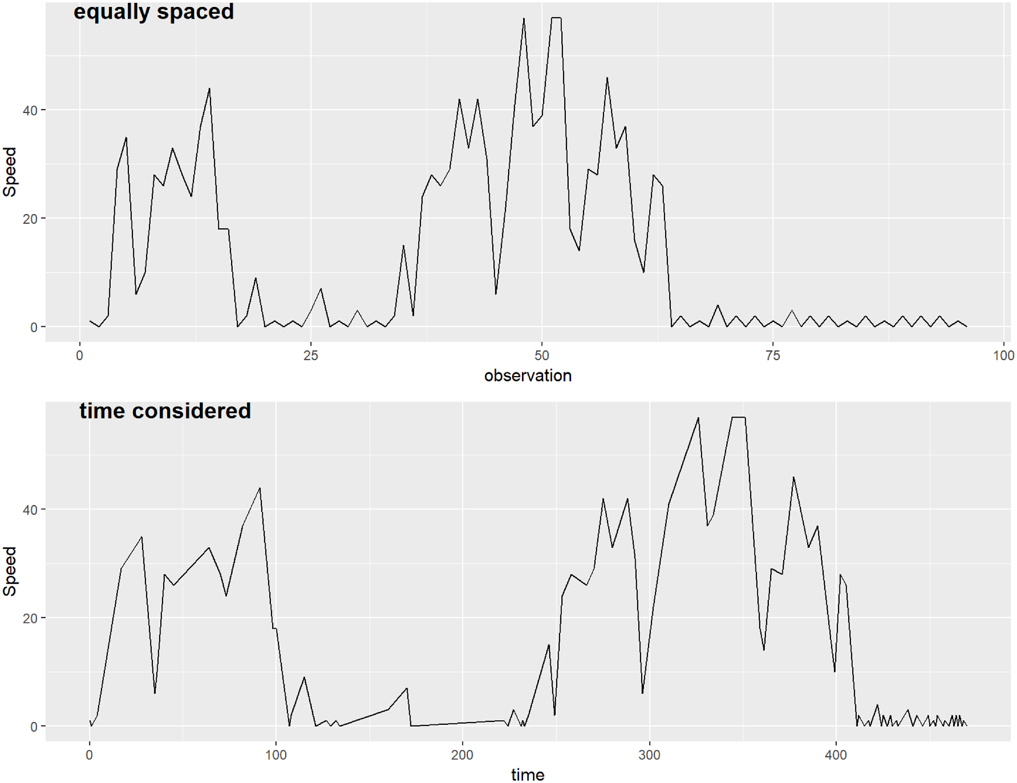
We observe that the patterns are similar, since the ‘significant’ changes should have been captured by curve logging. However, the interpretation can be different, especially if we would like to study the different driving behaviour, such as the magnitudes of acceleration and braking. In this example, we observe that first, changes can seem less or more abrupt than they actually are; and second, the small fluctuations at the end of the trip appear to have a much longer duration if observation times are not considered (around 40% of the entire trip vs. less than 25% of the trip).

Another challenge with the telematics records is that the trips (and their time series) are of different lengths. A possible solution is dynamic time warping (DTW), which is a technique to align, compare and measure the similarity of time series of different lengths. However, DTW requires regular time series, hence it is not directly applicable to our data unless the time series have been linearly interpolated.

The three aforementioned challenges demand a flexible, unsupervised time series model, which can incorporate time series irregularity and of varying lengths. We propose the use of a time-homogeneous CTHMM, where different states of the latent Markov chain will represent various driving actions and can be inferred via the observed telematics data. Together, all these states will describe the prevalent driving behaviour observed in the telematics data.

2.2. Data preparation

In particular, we model the following telematics responses: time (implicitly incorporated in the hidden Markov chain transitions), speed, and acceleration, which we further decompose into longitudinal (acceleration and braking) and lateral (left and right turning) components. Longitudinal acceleration reflects forward and backward movements, capturing braking and acceleration patterns, while lateral acceleration represents side-to-side movements, associated with cornering and swerving (Rajamani Reference Rajamani2012, Gillespie Reference Gillespie2020). This decomposition provides a more detailed characterization of driving behaviour, allowing us to distinguish between different driving styles and risk factors. For example, high longitudinal acceleration may indicate aggressive driving or stop-and-go traffic, whereas high lateral acceleration could suggest sharp cornering or sudden lane changes, which may result from reckless maneuvering or defensive evasive actions. Moreover, this separation enhances anomaly detection, enabling the model to identify distinct types of risky events rather than treating all acceleration events uniformly.

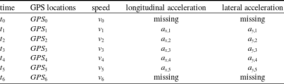
For illustrative purposes, let us consider a trip starting at time $t_0$ and ending at time $t_6$. We will employ the response alignments as shown in Table 1. To achieve the necessary structure, we first convert the GPS locations in latitude and longitude to Universal Transverse Mercator (UTM) coordinates, then we apply the following physics formula to obtain the longitudinal and lateral accelerations.

Table 1.

Telematics response alignments.

Let $\textbf{s} = (e, n)$ be the position of the vehicle at some time t, where e denotes the Easting and n denotes the Northing of the vehicle in UTM coordinates. From two consecutive UTM coordinates and the time interval in between, we calculate the velocity of the vehicle as

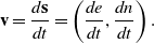$$ \textbf{v} = \frac{d\textbf{s}}{dt} = \left(\frac{de}{dt}, \frac{dn}{dt}\right).$$

In the case of discrepancy between this velocity and the GPS speed, velocity is scaled such that the magnitude matches the latter speed. Hence, velocity will be missing at the start of the trip. Then from two consecutive velocities, the acceleration is given by

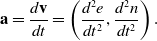$$ \textbf{a} = \frac{d\textbf{v}}{dt} = \left(\frac{d^2e}{dt^2}, \frac{d^2n}{dt^2}\right).$$

It is noteworthy that this acceleration is attributed to the initial time point $t_1$ as this is the (average) acceleration applied from time $t_1$ to $t_2$. Consequently, the acceleration values at both the start and end of the trip will be missing. Then the x-axis/longitudinal/tangential component of acceleration is

$$ a_x = \frac{\textbf{v} \cdot \textbf{a}} {||\textbf{v}||},$$

and the y-axis/lateral/normal component of acceleration is

$$ a_y = \sqrt{||\textbf{a}||^2 - a^2_x}.$$

3.1. Model description

The CTHMM is driven by a hidden Markov chain. A continuous-time hidden Markov chain with S discrete latent states is defined by an initial state probability distribution $\pi$ and a state transition rate matrix $\mathbf{Q}$. The elements $q_{uv}$ in $\mathbf{Q}$ describe the rate the process transitions from states u to v for $u \neq v$, $u, v = 1,...,S$, and $q_{uu} = - q_u = - \sum_{v\neq u} q_{uv}$. The chain is time homogeneous in the sense that $q_{uv}$ are independent of time t. The probability that the process transitions from states u to v is $q_{uv}/q_u$, while the sojourn time in state u follows an exponential distribution with rate $q_u$.

We assume drivers are independent, and each trip for a given driver is an independent time series generated from the CTHMM. To simplify the notation, we first consider a single trip j. At time point $t_l$, the available observed telematics data $\mathbf{y}_l$ depends on the current latent state $Z_l$ through the state-dependent distribution $f(\mathbf{y}_l | Z_l = z(t_l))$, where $z(t_l) \in \{1,2,...,S\}$ is the latent state at time $t_l$. Denote $\boldsymbol{\Phi} = (\pi, \mathbf{Q}, \boldsymbol{\Theta})$ the set of model parameters, where $\pi$ is the initial state probability distribution, $\mathbf{Q}$ is the transition rate matrix and $\boldsymbol{\Theta}$ are the parameters of the state-dependent distributions. If the continuous-time Markov model has been fully observed, meaning that one can observe every state transition time $\mathbf{T}' = (t'_0, t'_1, ..., t'_{T'})$, the corresponding states $\mathbf{Z}' = (z'_0 = z(t'_0), z'_1 = z(t'_1), ..., z'_{T'} = z(t'_{T'}))$, the observed data $\mathbf{Y} = (\mathbf{y}_0, \mathbf{y}_1, ..., \mathbf{y}_T)$ at observation time points $\mathbf{T} = (t_0, t_1, ..., t_T)$, then the complete data likelihood is

\begin{align*} \mathcal{L}(\boldsymbol{\Phi};\ \mathbf{Z}', \mathbf{T}', \mathbf{Y}, \mathbf{T}) &= \pi_{z'_0} \prod_{k=0}^{T' - 1} \left(\frac{q_{z'_{k}, z'_{k+1}}}{q_{z'_{k}}}\right)\left(q_{z'_{k}} \exp({-}q_{z'_{k}}(t'_{k+1} - t'_{k}))\right) \prod_{l=0}^T f(\mathbf{y}_l | Z_l = z(t_l)) \\ &= \pi_{z'_0} \prod_{u=1}^{S} \prod_{v=1, v\neq u}^{S} q_{uv}^{n_{uv}} \exp({-}q_u \tau_u) \prod_{l=0}^T f(\mathbf{y}_l | Z_l = z(t_l)),\end{align*}

where $n_{uv}$ is the number of transitions from states u to v and $\tau_u$ is the total time the chain remains in state u.

However in a realization of a CTHMM, there are two levels of hidden information. First, none of the states $\mathbf{Z}$ (at observation times) nor $\mathbf{Z}'$ (at transition times) are directly observed in the hidden Markov chain and can only be inferred from the observed data $\mathbf{Y}$. Second, the state transitions between two consecutive observations are also hidden– note the difference between state transition times $\mathbf{T}'$ and observation times $\mathbf{T}$. In other words, the chain may have multiple transitions before reaching a state which emits an observation. As a consequence, both $n_{uv}$ and $\tau_u$ are also unobserved. Here we assume the observed telematics process possesses the ‘snapshot’ property, such that the observation made at time $t_l$ depends only on the state active at time $t_l$, instead of the entire state trajectory over the interval $(t_{l-1},t_l]$ (Patterson et al., Reference Patterson, Parton, Langrock, Blackwell, Thomas and King2017).

We introduce two indicator functions: $\mathbb{1}_{\{Z_l = u\}} = 1$ if the latent state $z_l$ at observation time $t_l$ is u, and 0 otherwise; and $\mathbb{1}_{\{Z_l = u, Z_{l+1} = v\}} = 1$ if the latent states $z_l$, $z_{l+1}$ at observation times $t_l$ and $t_{l+1}$ are u and v, respectively, and 0 otherwise. The likelihood can be expressed instead as

\begin{equation*}\mathcal{L}(\boldsymbol{\Phi};\ \mathbf{Y}, \mathbf{T}) = \prod_{u=1}^S \pi_u ^{\mathbb{1}_{\{Z_0 = u\}}} \prod_{l=0}^{T - 1} \prod_{u,v=1}^S \mathbf{P}_{uv}(\Delta_{l+1})^{\mathbb{1}_{\{Z_l = u,Z_{l+1} = v\}}} \prod_{l=0}^T \prod_{u=1}^S f_u(\mathbf{y}_l)^{\mathbb{1}_{\{Z_l = u\}}},\end{equation*}

where $\mathbf{P}(t) = \exp(\mathbf{Q}(t))$ with $\Delta_l = t_l-t_{l-1}$ and matrix exponential $\exp$, and $f_u(\mathbf{y}_l) = f(\mathbf{y}_l | Z_l = u)$. $\mathbf{P}(t)$ is a state-transition matrix with the (u,v)-th entry $\mathbf{P}_{uv}(t)$, which is the probability that the (latent) Markov chain transitions from state u to state v after time t. It accounts for all possible intermediate state transitions which emit no observations happening before time t.

In an individual-specific model, where a distinct CTHMM is fitted for each individual, the complete data likelihood for a driver i with $N_i$ trips is given by

\begin{align*} \mathcal{L}_i \left(\boldsymbol{\Phi};\ \mathbf{Z}'^*, \mathbf{T}'^*, \mathbf{Y}^*, \mathbf{T}^* \right) &= \prod_{u=1}^{S} \prod_{v=1, v\neq u}^{S} q_{uv}^{\sum_{j=1}^{N_i} n_{ij,uv}} \exp\left({-}q_u \sum_{j=1}^{N_i} \tau_{ij,u}\right) \prod_{j=1}^{N_i} \pi_{z'_{ij0}} \prod_{l=0}^{T_{ij}} f \left(\mathbf{y}_{ijl} | Z_{ijl} = z(t_{ijl}) \right).\end{align*}

Alternatively, it can be represented as

\begin{equation*}\mathcal{L}_i(\boldsymbol{\Phi};\ \mathbf{Y}, \mathbf{T}) = \prod_{j=1}^{N_i} \left(\prod_{u=1}^S \pi_u ^{\mathbb{1}_{\{Z_{ij0} = u\}}} \prod_{l=0}^{T_{ij} - 1} \prod_{u,v=1}^S \mathbf{P}_{uv}(\Delta_{ij,l+1})^{\mathbb{1}_{\{Z_{ijl} = u,\;Z_{ij,l+1} = v\}}} \prod_{l=0}^{T_{ij}} \prod_{u=1}^S f_u(\mathbf{y}_{ijl})^{\mathbb{1}_{\{Z_{ijl}= u\}}}\right).\end{equation*}

In a pooled model, where a single CTHMM is trained to accommodate multiple individuals, each with $N_i$ trips for $i=1,...,M$, the complete data likelihood across all drivers is

\begin{align*} \mathcal{L}(\boldsymbol{\Phi};\ \mathbf{Z}'^*, \mathbf{T}'^*, \mathbf{Y}^*, \mathbf{T}^*) = \prod_{i=1}^M \mathcal{L}_i(\boldsymbol{\Phi};\ \mathbf{Z}'^*, \mathbf{T}'^*, \mathbf{Y}^*, \mathbf{T}^*),\end{align*}

or equivalently

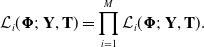\begin{equation*}\mathcal{L}_i(\boldsymbol{\Phi};\ \mathbf{Y}, \mathbf{T}) = \prod_{i=1}^M \mathcal{L}_i(\boldsymbol{\Phi};\ \mathbf{Y}, \mathbf{T}).\end{equation*}

The rationale for choosing between the individual-specific model and the pooled model will be discussed in Section 3.3.

While our modelling framework assumes independence across both drivers and trips by the same driver, the latter requires further consideration to assess its validity and implications. Rather than modelling each trip separately, we fit a single individual-specific CTHMM per driver, allowing all trips to contribute to learning that driver’s unique driving patterns. This ensures that recurring behaviour, such as tendencies in acceleration, braking, and cornering, is reflected in the estimated state transitions. As a result, while individual trips are treated as independent realizations from the same model, the model itself captures intra-driver dependencies by learning stable behavioural tendencies over time.

Although consecutive trips within a short time window (e.g., within the same day) may exhibit stronger correlations due to persistent road, weather, or driver conditions, variations still arise due to factors such as traffic conditions, driver fatigue, and trip purpose. These sources of randomness support the assumption that trips are drawn from the same underlying distribution but are not necessarily dependent on one another. Given that our focus is on long-term behavioural patterns and anomaly detection rather than short-term trip clustering, assuming independence across trips remains a reasonable and practical simplification for risk assessment.

If strong intra-driver dependence exists beyond what is captured by the driver-specific model, it may lead to an underestimation of variability in a driver’s risk profile. Future extensions could incorporate hierarchical models to explicitly account for temporal dependencies across trips, though at the cost of increased complexity. For this study, our approach balances model complexity and interpretability while effectively capturing key aspects of driver-specific behaviour, as will be demonstrated in the applications in Sections 5 and 6.

3.2. Anomaly detection

Interpreting the hidden states and their corresponding state-dependent distributions in a CTHMM can be challenging, especially when many states are needed to capture all significant combinations of the response dimensions. To illustrate this, Table 2 presents the state-dependent distributions from a 5-state individual-specific CTHMM for Driver 1 from the UAH-DriveSet (to be studied in detail in Section 5). Each row represents a latent state, and for instance, the last row (state 5) can be roughly interpreted as a driving action of ‘left turn (negative lateral acceleration) and deceleration (negative longitudinal acceleration) at a lower speed range (with the lowest mean speed of 81 $km/h$, though with a large standard deviation)’.

Table 2.

UAH-DriveSet: Summary of state-dependent distributions from a 5-state individual-specific CTHMM for D1. SD: standard deviation.

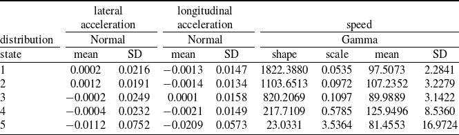
As shown in this example, a CTHMM with just 5 latent states for 3 response dimensions already requires interpreting 15 distributions. With fewer states, the distributions exhibit large standard deviations and significant overlap, making it unclear which driving action each state represents. Furthermore, certain driving actions may not be captured, e.g., lower speed ranges appear underrepresented in this example. Conversely, with more states, similar actions may be represented by multiple distributions, making it challenging to differentiate between them. More importantly, interpreting these latent states does not directly help achieve our goal of risk assessment, as associating states with driving risk levels is even more difficult and often subjective, especially in the absence of collision data. For example, Jiang and Shi (Reference Jiang and Shi2024) assumed specific accident probabilities associated with hard braking and big angle changes and simulated accidents based on these assumptions. As explained in Section 1, instead of focusing on specific accident-prone driving behaviour, we classify them broadly as ‘abnormal’ behaviour and propose to perform anomaly detection under a (fitted) CTHMM. Our proposed method is statistically supported and does not require explicit state interpretations, yet it can effectively identify outliers—in our case, the deviating driving behaviour.

Given a fitted CTHMM, we can perform anomaly detection on both entire trips and individual data points within a trip. Specifically, we utilize the ‘forecast pseudo-residuals’ introduced in Zucchini et al. (Reference Zucchini, MacDonald and Langrock2016). For a trip j from driver i at timepoint t, the uniform forecast pseudo-residual $u_{ijt,d}$ for the d-th dimension of the response $\textbf{Y}_{ijt}$, denoted as $Y_{ijt,d}$, is computed under the fitted model as

$$ u_{ijt,d} = P\left(Y_{ijt,d} \leq y_{ijt,d} \;|\; \textbf{Y}_{ij0} = \textbf{y}_{ij0}, \textbf{Y}_{ij1} = \textbf{y}_{ij1}, ..., \textbf{Y}_{ij,t-1} = \textbf{y}_{ij,t-1} \right).$$

In the context of HMMs, the analysis of pseudo-residuals serves two purposes: model checking and outlier detection, and we focus on the latter for this work. The forecast pseudo-residuals help identify observations that are extreme relative to the model and all preceding observations, highlighting the abrupt changes in driving behaviour. If a forecast pseudo-residual is extreme, it indicates that the corresponding observation is an outlier, or that the model no longer provides an acceptable description of the time series.

If the model fits the time series well, $u_{ijt,d}$ should follow a Uniform(0, 1) distribution, with extreme observations indicated by residuals close to 0 or 1. However, it can be hard to determine the extremity of a value under the uniform scale. For example, while a value of 0.97 might seem extreme on its own, it is less so when compared to 0.999. Consequently, Zucchini et al. (Reference Zucchini, MacDonald and Langrock2016) suggest using the normal forecast pseudo-residual

(1) \begin{equation} z_{ijt,d} = \Phi^{-1}\left(u_{ijt,d} \right),\end{equation}

where $\Phi$ is the standard normal cumulative density function. If the model is an accurate representation, $z_{ijt,d}$ should follow a standard normal distribution. In our analysis, we propose to classify observations with normal residuals exceeding 3 standard deviations as outliers. The 3-standard deviation threshold is widely used in statistical outlier detection, particularly for normally distributed data (Barnett and Lewis Reference Barnett and Lewis1994, Aggarwal Reference Aggarwal2015). This threshold is based on the empirical rule (also known as the 68-95-99.7 rule) for normal distributions. Flagging observations with residuals beyond 3 standard deviations—representing a 0.3% probability—effectively identifies points that are truly extreme relative to the model and preceding observations. We further examine the impact of threshold selection on anomaly detection performance in Section 5.2. Empirical results support the use of three standard deviations as the outlier threshold, as it effectively identifies anomalous trips and driving behaviour while maintaining a clear and consistent interpretation of what constitutes an extreme deviation from normal driving patterns.

Although we compute forecast pseudo-residuals $u_{ijt,d}$ and $z_{ijt,d}$ for each dimension d separately, all response dimensions influence these values, as $u_{ijt,d}$ is conditioned on the history across all dimensions. Consequently, the other dimensions also impact the probability of being in a particular latent state at each timepoint t.

In summary, our anomaly detection approach identifies deviations from learnt normal driving behaviour without predefining specific risky states (e.g., ‘aggressive’ or ‘drowsy’ driving). Instead, the model estimates the states in which a driver is most likely to be at a given time based on the (multivariate) telematics response, such as speed, longitudinal acceleration, and lateral acceleration in our analysis. Normal forecast pseudo-residuals $z_{ijt,d}$ are computed for each dimension d of telematics observations, and residuals beyond 3 standard deviations are flagged as outliers. At the trip level, we quantify the degree of anomaly by calculating the proportion of outliers in each dimension, defining this as the ‘anomaly index’. Rather than classifying certain states as inherently risky, our approach evaluates whether an individual is in an unexpected state given their usual driving patterns. This allows us to detect a broad range of abnormal behaviour without requiring predefined labels or assumptions about specific risk types, making the method both flexible and widely applicable.

3.3. Adapting and applying CTHMMs for anomaly detection in telematics

We perform anomaly detection at two levels to address two distinct objectives. At the driver level, we focus on identifying anomalous behaviour and trips that deviate from a driver’s typical patterns, particularly those associated with accidents. For this purpose, we use individual-specific models to account for heterogeneity in individual driving behaviour. Deng and Söffker (Reference Deng and Söffker2022) listed five factors influencing driving behaviour, which are driving styles, fatigue driving, drunk driving, driving skills, and traffic environment. Additional factors, such as vehicle characteristics, locations, and weather conditions, also play a role but are not available for consideration in our modelling. Lefèvre et al. (Reference Lefèvre, Carvalho, Gao, Tseng and Borrelli2015) compared the results of predicted acceleration and highlighted that a personalized/individualized model always outperforms an average/general model. While prediction is not our primary focus, the forecast pseudo-residuals in our approach calculate the predictive probability that a response dimension at the next time point is less extreme than the observed value given all previous observations. For reliable anomaly detection, the CTHMM must accurately capture a driver’s typical behaviour. A pooled model trained on data from multiple drivers may obscure individual anomalies, particularly for drivers whose deviations are minor within the group. Therefore, we fit individual-specific models to each driver’s trips to detect anomalies effectively.

At the group level, we aim to identify trips that deviate from the population norm and pinpoint drivers associated with at-fault claims. For this, we use a pooled model. While individual-specific models generate forecast pseudo-residuals to detect anomalies for each driver, these residuals may not be directly comparable across individuals. A pooled model, trained on trips from multiple drivers, enables us to compare trips across drivers, identify population-level anomalies, and rank drivers by their relative anomalousness.

For driver i with $N_i$ trips, the anomaly index for response dimension d in trip j with $T_{ij}+1$ observations is defined as:

(2) \begin{equation} A_{ij,d} = \frac{\sum_{t} \mathbb{1}(|z_{ijt,d}| \geq 3)}{T_{ij}}.\end{equation}

Note that the denominator is $T_{ij}$ only as forecast pseudo-residuals are not calculated at the first observation. To rank each driver’s trips by their level of anomalousness, we further define the normalized anomaly index, which is the ratio of each trip’s index to the maximum index for that driver:

(3) \begin{equation} \tilde{A}_{ij,d} = \frac{A_{ij,d}}{\max_j (A_{ij,d})}.\end{equation}

The (raw) anomaly indices for response dimension d across $N_i$ trips form an empirical distribution $\{A_{ij,d}, j = 1,...,N_i\}$ with empirical cumulative distribution function $F_{i,d}(p)$. For group-level analysis, we will focus on the right tail of this distribution, reflecting extreme anomaly levels in dimension d. In particular, the maximum and $\alpha$-th percentiles will be of interest:

$$ \max_{j}(A_{ij,d}) \quad \text{and} \quad P_{\alpha,d} = \inf\{p \,:\, F_{i,d}(p) \geq \alpha\}.$$

Although HMM is a flexible time-series model and the anomaly detection method is statistically grounded, there are several assumptions and adjustments that we need to make to adapt the proposed framework for the complex telematics data and ensure effective analysis.

1. 1. We assume that driving behaviour is predominately normal.

   • • While we aim to identify all abnormal driving behaviour, instead of focusing on just one or a few, we still assume that driving behaviour is mostly normal and safe. This means that for each driver, anomalous and risky trips are rare, and even within those risky trips (e.g., ones that result in accidents), abnormal driving instances occur infrequently. Consequently, the CTHMM, no matter individualized or generalized, is fitted to the normal and safe driving behaviour, with anomaly detection used to identify deviating ones. This assumption should be fair as accidents would no longer be rare events otherwise. As will be shown in Section 6.3, we tested pooled models with various portfolio compositions (having different claim rates), and the method proves robust regardless of the proportion of drivers with accidents the model is fitted on.

1. 2. The CTHMM should have a reasonable number of states.

   • • The CTHMM should have sufficient (latent) states to capture the major combinations of response dimensions, which ensures accurate modelling of a driver’s (in individual-specific models) and a group’s (in a pooled model) normal driving behaviour. However, it is equally important to avoid an excessive number of states, which can lead to model overfitting and mistakenly fitting well to abnormal behaviour as well. As a general guideline, we suggest starting with a number of latent states greater than the number of response dimensions (e.g., at least 5 states for 3 response dimensions) and increasing the number of states incrementally. The optimal number of states can then be selected based on Akaike information criterion (AIC) or Bayesian information criterion (BIC).

1. 3. We divide each trip into intervals of non-zero speed and assume these sub-intervals of each driver are independent time series generated from the same CTHMM.

   • • The forecast pseudo-residuals we consider for anomaly detection are based on probability integral transform, which applies to continuous distributions. While continuity adjustments can be made for discrete distributions, boundary points still pose problems. Harte (Reference Harte2021) pointed out that pseudo-residuals are poor indicators of the model goodness-of-fit when observations are near or at the boundary of the domain. Similarly, we find that under these conditions, pseudo-residuals are also ineffective at detecting outliers. Although we can model all values of speed with a semi-continuous distribution (e.g., a mixture of a continuous distribution on the positive real line and a point mass at 0), the boundary point 0 is problematic for anomaly detection. For this reason, we exclude 0-speed observations by dividing each trip into intervals of non-zero speed and non-missing accelerations, capturing moments when the driver is actually driving and the vehicle is moving. Consequently, we assume these sub-intervals (instead of trips) of each driver are independent time series generated by the same model and the CTHMM is fitted to sub-intervals. For analysis and anomaly detection, we still evaluate on a trip basis: we first compute the pseudo-residuals for each sub-interval, then aggregate the total number of outliers across all sub-intervals to compute the anomaly index (outlier proportion) for the trip; see Figure 2 and the description that follows for an illustration. By cutting trips into shorter, non-zero speed intervals, we aim to standardize the time series and reduce trip heterogeneity due to varying trip duration, road and weather condition, etc.

   • • Periods of low speed (near zero) may correspond to stops at traffic lights or other circumstances beyond the driver’s control and therefore may not be relevant for identifying anomalous driving behaviour. While excluding 0-speed intervals was necessary for effective outlier detection, this adjustment also mitigates the concern about such low-speed periods. By focusing on non-zero speed intervals, representing moments when the driver is actively driving and the vehicle is moving, this approach ensures that stopping events, such as waiting at traffic lights, do not influence the anomaly detection process.

4.1. E-step

At the m-th iteration, we first calculate the expected complete data loglikelihood

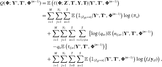(4) \begin{equation}\begin{split} Q(\boldsymbol{\Phi};\ \mathbf{Y}^*, \mathbf{T}^*, \boldsymbol{\Phi}^{(m-1)}) &= \mathbb{E}\left(\ell(\boldsymbol{\Phi};\ \mathbf{Z}', \mathbf{T}', \mathbf{Y}, \mathbf{T}) | \mathbf{Y}^*, \mathbf{T}^*, \boldsymbol{\Phi}^{(m-1)}\right) \\ &= \sum_{i=1}^M \sum_{j=1}^{N_i} \sum_{u=1}^S \mathbb{E}\left(\mathbb{1}_{\{Z_{ij0} = u\}} | \mathbf{Y}^*, \mathbf{T}^*, \boldsymbol{\Phi}^{(m-1)} \right) \log(\pi_u) \\ &\quad + \sum_{i=1}^M \sum_{j=1}^{N_i} \sum_{u=1}^S \sum_{v=1, v\neq u}^S \left\{ \log(q_{uv}) \mathbb{E}\left(n_{ij,uv}|\mathbf{Y}^*, \mathbf{T}^*, \boldsymbol{\Phi}^{(m-1)}\right) \right. \\ &\left. \qquad - q_{u} \mathbb{E} \left(\tau_{ij,u}|\mathbf{Y}^*, \mathbf{T}^*, \boldsymbol{\Phi}^{(m-1)} \right)\right\} \\ &\quad + \sum_{i=1}^M \sum_{j=1}^{N_i} \sum_{l=0}^T \sum_{u=1}^S \mathbb{E} \left(\mathbb{1}_{\{Z_{ijl} = u\}} | \mathbf{Y}^*, \mathbf{T}^*, \boldsymbol{\Phi}^{(m-1)} \right) \log\left(f_u(\mathbf{y}_{ijl}) \right),\end{split}\end{equation}

where $\mathbb{E}(\cdot|\mathbf{Y}^*, \mathbf{T}^*, \boldsymbol{\Phi}^{(m-1)})$ is the expected value given observed data $\mathbf{Y}^*$, observation times $ \mathbf{T}^*$ and the current estimate of model parameters $\boldsymbol{\Phi}^{(m-1)}$ resulted from the $(m-1)$-th iteration.

To simplify the notation, we first state the computation algorithms for a single trip sub-interval j from a driver i.

4.1.2. Soft decoding—Forward–backward algorithm

We define the forward probabilities $\boldsymbol{\alpha}_l$, backward probabilities $\boldsymbol{\beta}_l$ and likelihood $L_{T_j}$ (at time $T_j$) recursively as follows:

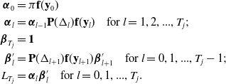\begin{align*} \boldsymbol{\alpha}_0 &= \pi \mathbf{f}(\mathbf{y}_0) \\ \boldsymbol{\alpha}_l &= \boldsymbol{\alpha}_{l-1} \mathbf{P}(\Delta_l) \mathbf{f}(\mathbf{y}_l) \quad \text{for } l=1,2,...,T_j;\\ \boldsymbol{\beta}_{T_j} &= \mathbf{1} \\ \boldsymbol{\beta}'_l &= \mathbf{P}(\Delta_{l+1}) \mathbf{f}(\mathbf{y}_{l+1})\boldsymbol{\beta}'_{l+1} \quad \text{for } l=0,1,...,T_j-1;\\ L_{T_j} &= \boldsymbol{\alpha}_l \boldsymbol{\beta}'_l \quad \text{for } l=0,1,...,T_j.\end{align*}

Then we can define the ‘smoother’ for $l=0,1,...,T_j$

(5) \begin{equation} \mathbb{E}\left(\mathbb{1}_{\{Z_l = u\}} | \mathbf{Y}^*, \mathbf{T}^*, \boldsymbol{\Phi}^{(m-1)} \right) = \frac{\boldsymbol{\alpha}_l[u] \boldsymbol{\beta}_l[u]}{L_{T_j}},\end{equation}

where $\boldsymbol{\alpha}_l[u]$ and $\boldsymbol{\beta}_l[u]$ are the u-th elements in the vectors $\boldsymbol{\alpha}_l$ and $\boldsymbol{\beta}_l$, respectively.

To this end, we also define the ‘two-slice marginal’ for $l=0,1,...,T_j-1$, which will be used in the computation in Section 4.1.2,

(6) \begin{equation} \mathbb{E} \left(\mathbb{1}_{\{Z_l = u, Z_{l+1} = v\}} | \mathbf{Y}^*, \mathbf{T}^*, \boldsymbol{\Phi}^{(m-1)} \right) = \frac{\boldsymbol{\alpha}_l[u] \mathbf{P}(\Delta_{l+1})[u,v]\, f_v(\mathbf{y}_{l+1})\boldsymbol{\beta}_{l+1}[v]}{L_{T_j}},\end{equation}

where $\mathbf{P}(\Delta_{l+1})[u,v]$ is the (u,v)-th element of $\mathbf{P}(\Delta_{l+1})$.

4.1.3. Hard decoding—Viterbi algorithm

We first construct two S-by-$(T_j+1)$ matrices $\mathbf{V}_1$ and $\mathbf{V}_2$ with their (u,l)-th elements as follows:

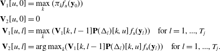\begin{align*} \mathbf{V}_1[u,0] &= \max_k (\pi_k f_u(\mathbf{y}_0)) \\ \mathbf{V}_2[u,0] &= 0 \\ \mathbf{V}_1[u,l] &= \max_k (\mathbf{V}_1[k,l-1] \mathbf{P}(\Delta_{l})[k,u]\, f_u(\mathbf{y}_l)) \quad \text{for } l=1,...,T_j\\ \mathbf{V}_2[u,l] &= {\arg\max}_k (\mathbf{V}_1[k,l-1] \mathbf{P}(\Delta_{l})[k,u]\, f_u(\mathbf{y}_l)) \quad \text{for } l=1,...,T_j.\\\end{align*}

Then we backtrack to find the most likely sequence of latent states:

\begin{align*} \hat{z}_{T_j} &= {\arg\max}_k (\mathbf{V}_1[k,T_j]) \\ \hat{z}_{l-1} &= \mathbf{V}_2(\hat{z}_l,l) \quad \text{for } l=1,...,T_j.\end{align*}

We can define the ‘smoother’ for $l=0,1,...,T_j$

(7) \begin{equation} \mathbb{E}\left(\mathbb{1}_{\{Z_l = u\}} | \mathbf{Y}^*, \mathbf{T}^*, \boldsymbol{\Phi}^{(m-1)} \right) = \mathbb{1}_{\{\hat{z}_l=u\}},\end{equation}

and the ‘two-slice marginal’ for $l=0,1,...,T_j-1$

(8) \begin{equation} \mathbb{E}\left(\mathbb{1}_{\{Z_l = u, Z_{l+1} = v\}} | \mathbf{Y}^*, \mathbf{T}^*, \boldsymbol{\Phi}^{(m-1)} \right) = \mathbb{1}_{\{\hat{z}_l=u, \hat{z}_{l+1}=v\}}.\end{equation}

4.1.4. Conditional expectations of $n_{uv}$ and $\tau_{u}$

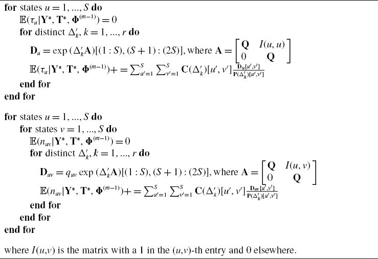
The complication in the E-step lies in the calculation of $\mathbb{E}(n_{uv}|\mathbf{Y}^*, \mathbf{T}^*, \boldsymbol{\Phi}^{(m-1)})$ and $\mathbb{E}(\tau_{u}|\mathbf{Y}^*, \mathbf{T}^*, \boldsymbol{\Phi}^{(m-1)})$. We make use of the Expm algorithm proposed by Liu et al. (Reference Liu, Li, Li, Song and Rehg2015), which provides an efficient way for computing integrals of matrix exponentials; it is restated in Algorithm 1.

The algorithm exploits the fact that the hidden Markov chain is time-homogeneous and the state-transition matrix at any timepoint $t_{l-1}$, $\mathbf{P}(\Delta_l)$, only depends on the time interval between now and the next observation timepoint $\Delta_l = t_l - t_{l-1}$. As a consequence, the conditional expectations of $n_{ij,uv}$ and $\tau_{ij,u}$ only have to be evaluated for each distinct time interval rather than at each observation time. We denote $\Delta'_k, k=1,...,r,$ the r distinct values of $\Delta_l, l=1,...,T_j$, and create count tables $\mathbf{C}(\Delta'_k)$ with the two-slice marginals from Equation 6 or Equation 8 as

$$ \mathbf{C}(\Delta'_k)[u,v] = \sum_{l: \Delta_l = \Delta'_k} \mathbb{E}\left(\mathbb{1}_{\{Z_l = u, Z_{l+1} = v\}} | \mathbf{Y}^*, \mathbf{T}^*, \boldsymbol{\Phi}^{(m-1)} \right).$$

Algorithm 1

Expm Algorithm for Computing $\mathbb{E} \left(\tau_{u}|\mathbf{Y}^*, \mathbf{T}^*, \boldsymbol{\Phi}^{(m-1)} \right)$ and $\mathbb{E} \left(n_{uv}|\mathbf{Y}^*, \mathbf{T}^*, \boldsymbol{\Phi}^{(m-1)} \right)$

4.2. M-step

The goal of the M-step is to maximize $Q(\boldsymbol{\Phi};\ \mathbf{Y}^*, \mathbf{T}^*, \boldsymbol{\Phi}^{(m-1)})$ with respect to $\boldsymbol{\Phi}$. However, it is too computational costly to directly find the global maximum. Instead, we aim to use a computational effective algorithm to find a near-maximum to update the parameters $\boldsymbol{\Phi}^{(m)}$ such that $Q(\boldsymbol{\Phi}^{(m)};\ \mathbf{Y}^*, \mathbf{T}^*, \boldsymbol{\Phi}^{(m-1)}) \geq Q(\boldsymbol{\Phi}^{(m-1)};\ \mathbf{Y}^*, \mathbf{T}^*, \boldsymbol{\Phi}^{(m-1)})$. It follows from Equation 4 that $Q(\boldsymbol{\Phi};\ \mathbf{Y}^*, \mathbf{T}^*, \boldsymbol{\Phi}^{(m-1)})$ can be decomposed into three parts

$$ Q(\boldsymbol{\Phi};\ \mathbf{Y}^*, \mathbf{T}^*, \boldsymbol{\Phi}^{(m-1)}) = Q^{(m)}_{\pi} + Q^{(m)}_{\mathbf{Q}} + Q^{(m)}_{\boldsymbol{\Theta}},$$

where

(9) \begin{align} Q^{(m)}_{\pi} &= \sum_{i=1}^M \sum_{j=1}^{N_i} \sum_{u=1}^S \mathbb{E}\left(\mathbb{1}_{\{Z_{ij0} = u\}} | \mathbf{Y}^*, \mathbf{T}^*, \boldsymbol{\Phi}^{(m-1)} \right) \log(\pi_u); \\[-24pt] \nonumber \end{align}

(10) \begin{align} Q^{(m)}_{\mathbf{Q}} &= \sum_{i=1}^M \sum_{j=1}^{N_i} \sum_{u=1}^S \sum_{v=1, v\neq u}^S \left\{ \log(q_{uv}) \mathbb{E} \left(n_{ij,uv}|\mathbf{X}^*, \mathbf{Y}^*, \mathbf{T}^*, \boldsymbol{\Phi}^{(m-1)} \right) - q_{u} \mathbb{E} \left(\tau_{ij,u}| \mathbf{Y}^*, \mathbf{T}^*, \boldsymbol{\Phi}^{(m-1)} \right)\right\};\ \text{and} \\[-24pt] \nonumber \end{align}

(11) \begin{align} Q^{(m)}_{\boldsymbol{\Theta}} &= \sum_{i=1}^M \sum_{j=1}^{N_i} \sum_{l=0}^{T_j} \sum_{u=1}^S \mathbb{E} \left(\mathbb{1}_{\{Z_{ijl} = u\}} | \mathbf{Y}^*, \mathbf{T}^*, \boldsymbol{\Phi}^{(m-1)}\right) \log\left(f_u(\mathbf{y}_{ijl})\right) .\end{align}

Clearly, $Q^{(m)}_{\pi}$ depends only on $\pi$, $Q^{(m)}_{\mathbf{Q}}$ depends only on $\mathbf{Q}$, and $Q^{(m)}_{\boldsymbol{\Theta}}$ depends only on $\boldsymbol{\Theta}$. As a consequence, the problem reduces to maximize the three functions separately with respect to the corresponding subset of parameters. While we can compute the E-step for each trip sub-interval separately, we have to consider all of them collectively in the M-step calculation.

4.2.1. Initial state probability distribution $\pi$

We constrain $\pi_u$ summing to unity by use of a Lagrange multiplier. Then by taking the derivative of $Q^{(m)}_{\pi}$ with respect to $\pi_u$, we have the maximum likelihood estimator (MLE) in the m-th iteration as

$$ \pi^{(m)}_u = \frac{\sum_{i=1}^M \sum_{j=1}^{N_i} \mathbb{E} \left(\mathbb{1}_{\{Z_{ij0} = u\}} | \mathbf{X}^*, \mathbf{Y}^*, \mathbf{T}^*, \boldsymbol{\Phi}^{(m-1)} \right)}{\sum_{u'=1}^S \sum_{i=1}^M \sum_{j=1}^{N_i} \mathbb{E}\left(\mathbb{1}_{\{Z_{ij0} = u'\}} | \mathbf{X}^*, \mathbf{Y}^*, \mathbf{T}^*, \boldsymbol{\Phi}^{(m-1)}\right)}.$$

4.2.2. Transition rate matrix $\mathbf{Q}$

By taking the derivative of $Q^{(m)}_{\mathbf{Q}}$ with respect to $q_{uv}$ for $u \neq v$, we have the MLE in the m-th iteration as

$$ q^{(m)}_{uv} = \frac{\sum_{i=1}^M \sum_{j=1}^{N_i} \mathbb{E} \left(n_{ij,uv}|\mathbf{Y}^*, \mathbf{T}^*, \boldsymbol{\Phi}^{(m-1)}\right)}{\sum_{i=1}^M \sum_{j=1}^{N_i} \mathbb{E}\left(\tau_{ij,u}|\mathbf{Y}^*, \mathbf{T}^*, \boldsymbol{\Phi}^{(m-1)}\right)} \quad \text{and} \quad q^{(m)}_{uu} = - q^{(m)}_{u} = - \sum_{v\neq u} q^{(m)}_{uv}.$$

4.3. Joint modelling of telematics and computational cost

In this work, we analyse multivariate time series of speed, longitudinal acceleration and lateral acceleration. Joint modelling of telematics responses provides a more complete picture of driving behaviour while also enhancing anomaly detection. Although it increases computational complexity, it provides a more comprehensive and robust risk assessment compared to analysing each variable separately.

One key advantage of joint modelling is that it captures the interactions between different telematics responses, leading to a more complete representation of driving behaviour. Speed and acceleration complement each other, offering richer context than when analysed individually. For instance, the same acceleration intensity at different speed ranges may indicate very different driving conditions: a harsh acceleration at low speeds could be a normal response in stop-and-go traffic, whereas the same acceleration at high speeds might signal aggressive driving.

Beyond improving behavioural modelling, joint modelling significantly enhances anomaly detection. As will be demonstrated in Section 5.2 (Tables 5 and 6), outlier identification depends not only on a single variable but on the combination of speed and acceleration components. Since pseudo-residual calculations and anomaly detection are influenced by which latent state is the most probable at each time point, and it depends on the other response dimensions as well, excluding key response dimensions weakens the model’s ability to identify true behavioural anomalies.

The trade-off between predictive accuracy and computational complexity primarily comes from an increase in the number of latent states. For example, if speed and longitudinal acceleration are each categorized into three levels (low, mid, and high), a univariate CTHMM requires only 3 states, while a multivariate model may require 9 states. However, if both univariate and multivariate models are constrained to the same number of states, the multivariate model does not introduce significant additional computational costs. Under the assumption of conditional independence of response dimensions given a state, likelihood calculations remain computationally efficient as they only involve the multiplication of density functions across dimensions.

5.1. Data description

Before applying our CTHMM-based anomaly detection to the real-world dataset that lacks labels for driving behaviour, we first evaluate its effectiveness using a labelled telematics dataset. Specifically, we analyse the UAH-DriveSet (Romera et al., Reference Romera, Bergasa and Arroyo2016), a publicly available telematics dataset. This dataset consists of six drivers, each driving a different vehicle, performing three distinct driving behaviour (normal, aggressive, and drowsy) on two different roads (a motorway and a secondary road). While the dataset contains extensive telematics information and even video recordings, our controlled study focuses on validating the proposed method’s ability to detect abnormal driving behaviour, ensuring that it can be applied to the real-world data for risk evaluation. For this purpose, we limit our analysis to the same set of telematics features, which are speed, longitudinal, and lateral accelerations only.

In the UAH-DriveSet, telematics recording starts when the vehicle enters the specific road and ends when it exits, hence speed is always non-zero, posing no issues for anomaly detection as discussed in Section 3.3. Speed is collected from GPS at 1Hz, while accelerations are recorded from accelerometer at 10Hz. According to Romera et al. (Reference Romera, Bergasa and Arroyo2016), ‘Z’ and ‘Y’ denote the longitudinal and lateral accelerations, respectively. Since accelerometers are sensitive and measurements can be noisy, we consider ‘Z_KF’ and ‘Y_KF’, which have been filtered by a Kalman Filter and are readily available in the dataset. We downsample the 3-dimensional responses such that they are all observed per second. Although one can apply a discrete-time HMM to this data due to its regular time intervals, we apply the continuous-time version to also test that the model estimation algorithm runs correctly.

On the motorway, each driver performed three round trips, simulating each of the three driving behaviour. On the secondary road, each of them performed four one-way trips, consisting of both a departure and a return as normal, a departure as aggressive and a return as drowsy. Hence, each driver should have telematics records of seven trips. In the following discussion, we omit driver D6 who drove an electric vehicle, since he did not perform the aggressive trip on the secondary road due to lack of autonomy.

While the road type is available in the UAH-DriveSet (in fact, drivers are not only driving on two specific road types but two designated roads), road types are not always available in real data. In reality, trips tend to be longer and can involve various road types. For example, a driver who commutes to work from home can have travelled on all of residential streets, primary to tertiary roads, and motorways, and it can be difficult to assign a single road type to such a trip. For this reason, we do not consider road types in the controlled study; yet, we will show that results demonstrate strong model performance.

5.2. Individual-specific model

We first test the ability of individual-specific models in identifying anomalous trips for each driver, with a particular focus on detecting the two aggressive trips as a representative example. For each of the drivers D1 to D5, we fit a 20-state CTHMM to his/her seven trips. We tested a limited selection of models with 5, 10, 15, 20, and 25 states, with 20 states being optimal according to both AIC and BIC. This choice ensures that the model captures all major combinations of speed and accelerations without overfitting. More discussions on the robustness of the results with respect to the number of states are presented later in this subsection.

The state-dependent distributions are gamma for speed and normal for both longitudinal and lateral accelerations. These choices are made based on the domain and characteristics of each response dimension. Gamma distribution is right-skewed and strictly positive, making it well-suited for modelling speed, which is often asymmetric with a long tail at higher values. Additionally, it has two parameters (shape and scale), allowing it to adapt to different degrees of skewness and dispersion in speed distributions. Normal distribution is appropriate for acceleration because acceleration values are often symmetrically distributed around zero, with both positive (acceleration) and negative (deceleration) values. It is also widely used due to its tractable properties and well-established estimation methods. In addition to optimizing the number of latent states, one can also explore alternative choices for state-dependent distributions. For example, a 20-state CTHMM could be fitted using either log-normal or gamma distributions for speed, with model selection guided by AIC or BIC. This flexibility allows for further refinement of the model based on empirical fit.

Initial guesses for parameter estimation are important in EM algorithm as they can influence the convergence of the algorithm and the final model fit, especially in the case when the algorithm converges to a local optimum instead of a global one. Parameter initializations of $\pi$ and $\mathbf{Q}$ are random, while state-dependent distribution parameters $\boldsymbol{\Theta}$ are initiated with k-means clustering. Users are encouraged to try multiple different initializations to reduce the chances of the model converging to a local optimum. To robustify our analysis, we re-fit the model 100 times with different random initializations and analyse the average result.

After model fitting, we calculate the anomaly indices of each trip under the corresponding driver’s model. The results are reported in Table 3. First, we observe that trips performed on motorway usually have some outliers in speed. This is expected as the driving speed is generally higher on motorway than on secondary road. However, speed alone does not reveal the driving behaviour, and it is essential to consider the changes of it, which are the accelerations. Second, we observe that the two aggressive trips are characterized by the higher anomaly index in the longitudinal acceleration (acceleration and braking). This is in line with the experiment set-up: the drivers are told to push to the limit their aggressiveness without putting the vehicle at risk. Furthermore, this is also in line with Zylius et al. (Reference Zylius, Vaitkus and Lengvenis2014), which showed that aggressive and safe driving styles can be more effectively classified using longitudinal acceleration signals. While longitudinal acceleration is clearly associated with aggressiveness, the relationship between lateral acceleration and driving behaviour is less straightforward. However, as we will demonstrate in Section 6, anomaly indices for both longitudinal and lateral accelerations show a positive correlation with accident probability.

Table 3.

UAH-DriveSet: Anomaly index in each dimension of telematics observations, computed from individual-specific CTHMMs with 20 states for each driver and averaged over 100 random initializations. Note: S stands for Secondary Road and M stands for Motorway; Z and Y are longitudinal and lateral accelerations, respectively.

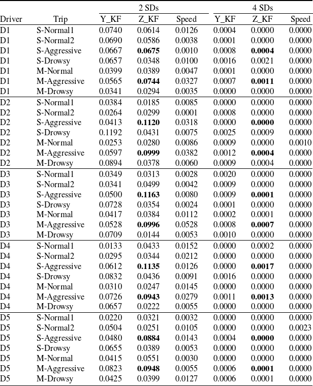
While the anomaly index with the proposed outlier threshold of 3 standard deviations (SDs) provides strong anomaly detection results, we further examine the impact of threshold selection on performance. Table 4 presents the anomaly indices computed using alternative outlier thresholds of 2 and 4 SDs. Using a lower (higher) threshold increases (decreases) the anomaly index. We observe that with a 2-SD threshold, the two aggressive trips for each driver still exhibit higher anomaly indices in longitudinal acceleration and can be identified. However, with a 4-SD threshold, many indices drop close to zero, as it becomes highly unlikely for a normal forecast pseudo-residual to exceed 4 in absolute magnitude. As a result, the two aggressive trips can no longer be distinguished from other trips. Furthermore, while the 2-SD threshold still identifies the aggressive trips, it results in anomaly indices that are approximately 10 times higher than those computed with a 3-SD threshold (Table 3). This raises concerns about whether the trips are truly that anomalous and whether the anomaly index retains its intended meaning. For instance, under the 2-SD threshold, normal trips on the secondary road have an average of 3.84% outliers, whereas under the 3-SD threshold, this drops to 0.82%, which more accurately reflects them as following normal driving behaviour. These observations support the use of 3 standard deviations as the outlier threshold, as it effectively identifies anomalous trips and driving behaviour while maintaining interpretability.

Table 4.

UAH-DriveSet: Alternative thresholds (2 and 4 standard deviations (SDs)) for calculating anomaly index in each dimension of telematics observations, computed from individual-specific CTHMMs with 20 states for each driver and averaged over 100 random initializations. Note: S stands for Secondary Road and M stands for Motorway; Z and Y are longitudinal and lateral accelerations, respectively.

Table 5.

Snapshot of D1’s aggressive trip on motorway with pseudo-residuals of Z_KF. Note: Z and Y are longitudinal and lateral accelerations, respectively.

Table 6.

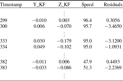
Snapshot of D2’s aggressive trip on motorway with pseudo-residuals of Z_KF. Note: Z and Y are longitudinal and lateral accelerations, respectively.

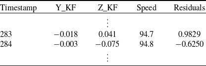
It is worth mentioning that pseudo-residuals consider more than just the magnitudes of the responses—they also take into account information derived from the other dimensions of the response and how likely the observed transitions are. Table 5 includes a snapshot of D1’s aggressive trip performed on the motorway, with pseudo-residuals of longitudinal acceleration Z_KF. First, we see that the longitudinal acceleration (−0.070) at timepoint 300 is an outlier, despite having a magnitude smaller than that (−0.102) at timepoint 334, which is not an outlier. This is because the first transition is from a less extreme value (0.003) to a more extreme one, while the second transition is the other way around. Second, we also observe that the longitudinal acceleration (−0.070) at timepoint 300 is an outlier while that (−0.086) at timepoint 383 is not despite having transitions of similar magnitude. The reason is that the speed during the latter transition is in a different range, and such transitions are more common in the lower speed range for this driver. Furthermore, since model training and analysis are performed on a per-driver basis rather than collectively, how likely a transition is, and consequently the identification of outliers, also varies across drivers. Outliers cannot be identified through direct comparison between drivers. For example, Table 6 provides a snapshot of D2’s aggressive trip performed on the motorway. If we compare this transition with D1’s first (selected) transition, we see that despite having similar speed, comparable resulting longitudinal acceleration, and an arguably more aggressive transition (from 0.041 to -0.075 as compared to from 0.003 to -0.070), it is not an outlier while D1’s transition is. This is due to the fact that such transitions are more typical in D2’s driving history but not as much for D1.

While the above analysis uses CTHMMs with 20 states, we also explore the effect of different number of states on the results. For simplicity, we consider a limited selection of 5, 10, 15, 20, and 25 states. For each number of states, we re-fit the model 100 times with different random initializations and compute the average results. Since the models with 25 states include degenerate state-dependent distributions for accelerations, we do not report their results and terminate the search at 20 states, which gives the lowest AIC and BIC. With increasing number of states, we observe that the anomaly indices generally decrease, as more telematics combinations are described and fewer data points are then considered outliers. The two aggressive trips are consistently characterized by more outliers in longitudinal acceleration, except for Driver 1, where there is a mix between the two aggressive trips and the drowsy trip completed on the secondary road when the number of states is lower. Detailed results can be found in Appendix B.

Using the UAH-DriveSet, we have validated that the proposed individual-specific CTHMM, along with its anomaly detection method, effectively learns and distinguishes between different driving behaviour. With minimal supervision— specifying only the number of states and the state-dependent distribution families—the fitted model is able to capture key combinations of speed and accelerations and identify deviating behaviour. The model achieves this by considering not only speed but also its changes, and more importantly their combinations. We expect that speed inherently captures information regarding road type, and driving behaviour (normal, aggressive, and drowsy) is then described by its combination with lateral and longitudinal accelerations.

Compared to the state-of-the-art methods applied to the UAH-DriveSet, this work introduces several methodological advancements and distinctions. Existing studies primarily rely on supervised machine learning techniques, leveraging labelled data to classify aggressive driving behaviour using methods such as convolutional neural networks (CNNs), recurrent neural networks (RNNs), and ensemble models. Moreover, these approaches typically incorporate diverse telematics inputs, including GPS data, gyroscope readings, and even video recordings, to enhance feature richness and classification accuracy (Romera et al. Reference Romera, Bergasa and Arroyo2016, Moukafih et al. Reference Moukafih, Hafidi and Ghogho2019, Liu et al. Reference Liu, Lu, Liao, Qiao, Zhang, Zhu, Xu and Li2024). In contrast, we introduce an unsupervised anomaly detection method under the CTHMM, addressing the practical challenge of label unavailability in real-world scenarios. Furthermore, this work demonstrates the robustness of using only three fundamental telematics responses: speed, longitudinal acceleration, and lateral acceleration. This much simpler yet effective approach highlights the adaptability of the proposed methodology to datasets with limited sensor information while maintaining strong capabilities in anomaly detection and aggressive trip identification.

5.3. Pooled model

As shown in the previous section, individual-specific models can produce forecast pseudo-residuals that effectively highlight anomalous trips for each driver. However, there is no guarantee that these residuals can be compared across different individuals as they are derived from distinct models. Therefore, we employ a pooled model that enables trip comparison across individuals and driver rankings.

We train a 20-state CTHMM using all 35 trips from the five drivers D1 to D5. The state-dependent distributions and parameter initializations match those used in the individual-specific models. After model fitting, we assess the anomaly indices of each trip under the pooled model. To enhance the robustness of our analysis, we also re-fit the model 100 times with different random initializations and present the average result in Table 7.

Table 7.

UAH-DriveSet: Anomaly index in each dimension of telematics observations, computed from pooled CTHMM with 20 states from all drivers and averaged over 100 random initializations. Note: S stands for Secondary Road and M stands for Motorway; Z and Y are longitudinal and lateral accelerations, respectively.

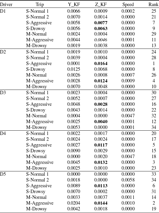
First, when comparing the 7 trips of each driver, we observe that the two aggressive trips again exhibit a higher anomaly index in longitudinal acceleration, except for D1, where there is once more a mix between the two aggressive trips and the drowsy trip driven on the secondary road. Second, since the pseudo-residuals are derived from the same pooled models, we can now fairly compare them and rank the trips. Table 7 also presents the ranking of each trip among all 35, in descending anomaly index in longitudinal acceleration. D2’s aggressive trip on the secondary road ranks highest in terms of anomalousness in longitudinal acceleration (or aggressiveness), followed by D5’s aggressive trip on the motorway. Lastly, due to heterogeneity in individual driving behaviour, it is possible for a driver’s normal trip to be deemed more anomalous than another driver’s abnormal trip. For instance, D5’s normal trip on the motorway exhibits a higher anomaly index in longitudinal acceleration compared to D3’s aggressive trip on the secondary road.

While the intermediate rankings of trips may not be completely clear, it is obvious that D2 is the most aggressive driver, while D3 is the least. Although both drivers are male and in the 20–30 age range, they drive different vehicles. D2 drives a Mercedes B180 (2013), a compact yet relatively powerful vehicle, which could encourage more aggressive driving, particularly on secondary roads. In contrast, D3 drives a Citroën C4 (2015), a smaller and potentially less powerful car, which could lead to a more cautious driving style. These differences in vehicle characteristics likely influence their respective driving behaviours.

However, we lack ground-truth labels regarding the anomalousness or riskiness of each driver, as none has been involved in accidents. While we have outlined a method in this section and demonstrated its use, we admit that we cannot fully validate the rankings presented above. We keep this issue in mind, but the observed patterns—such as D2’s higher anomaly index indicating more aggressive driving among the group of drivers—are suggestive. We aim to validate our findings further in Section 6.3 using the rental car dataset.

6.1. Data description

We now apply our proposed CTHMM to the rental car dataset, which contains claims reported from January 1, 2019 to January 31, 2023. As we would like to investigate the connection between driving behaviour and accidents, we focus on at-fault claims. These claims are typically more directly related to driver actions and behaviour and are expected to provide greater insight into how these factors contribute to accidents. The portfolio includes 1,678 rentals with at least one at-fault claim and 16,495 rentals without claims.

Recall that one challenge with this dataset is the lack of precise labels for accident-associated trips. Claims are reported with a date of loss but not the specific trip involved. To approximate these labels, we rely on ‘potential accident triggers’ provided by our collaborator, who specializes in both telematics recording hardware and software development. In big lines, these triggers are derived based on predefined thresholds on accelerometer readings and further inspections on speed changes (e.g., whether the vehicle comes to a stop afterwards).

However, the method used by our collaborator is not perfect. While these triggers are accurate in distinguishing between real crashes and harsh braking events, they suffer from a high false-negative rate due to curve logging (explained in Section 2), which also applies to accelerometer readings. Curve logging reduces noise in the accelerometer readings, but may unintentionally filter out some acceleration values that exceed the thresholds. As a result, only about 10% of the at-fault claims are matched with a corresponding trigger, leaving the remaining 90% unassociated with specific trips—even though we know these claims exist.

Given this limitation, we treat the detected triggers as ground truth. Since the date of loss is customer-reported and may not be fully reliable, we extend the analysis to consider all trips completed within a 3-day window (the date of loss, plus the day before and after). While we are certain that 1,678 trips are associated with accidents (corresponding to the 1,678 at-fault claims), only 94 of them are identified by our collaborator’s method. These 94 trips are referred to as ‘target trips’ and are treated as the ground truth for our analysis. The challenge we address with the individual-specific models is whether our method can correctly identify these 94 target trips as being accident related. The number of trips per 3-day window (around date of loss) ranges from 2 to 63, with an average of 18 trips, totalling 1,765 trips. In summary, the goal of the individual-specific model is to identify the 94 target trips that correspond to actual claims and accidents from the pool of 1,765 trips.

Figure 2.

Speed time series (in $km/h$) of a sample trip. Shaded regions indicate intervals of non-zero speed, where all intervals are used for anomaly detection, but only the blue ones are used for model fitting.

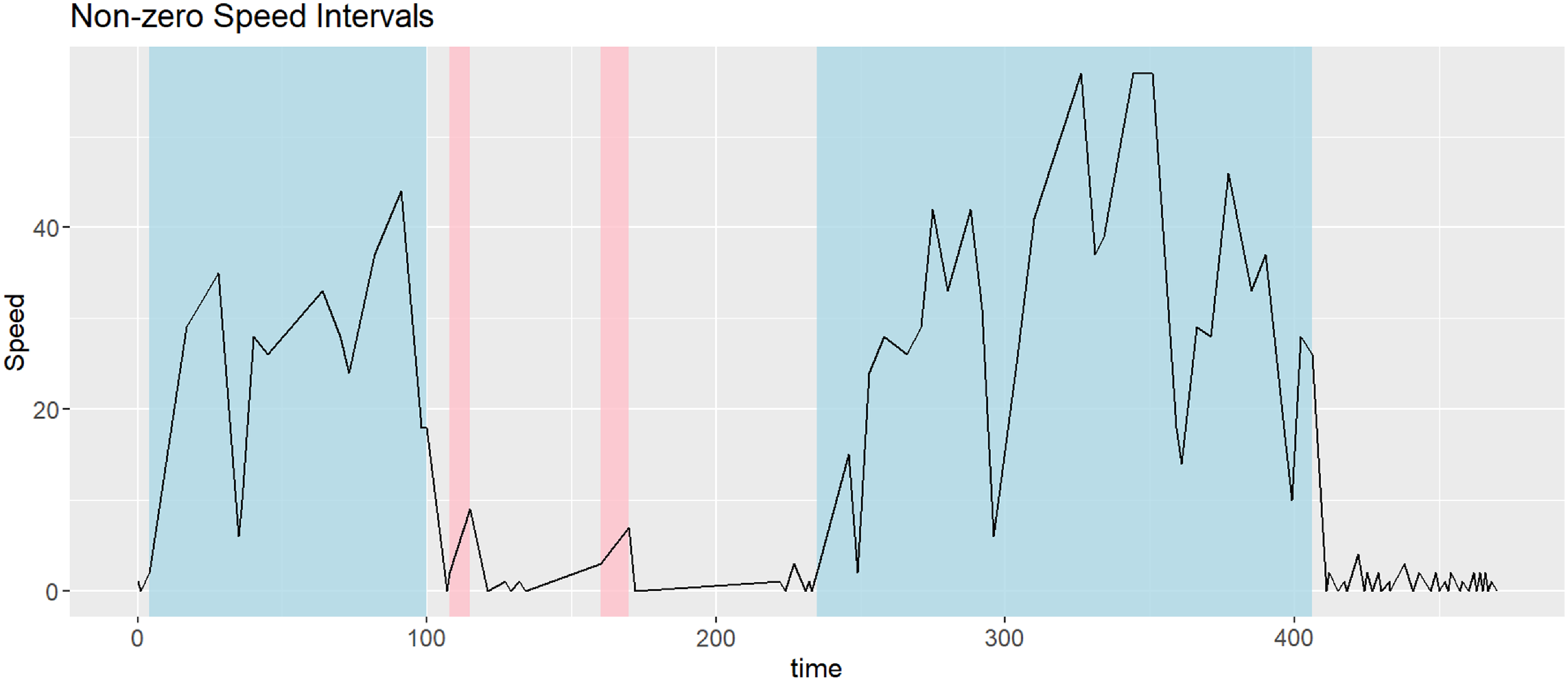
For both individual-specific and pooled models, telematics data undergo the same preprocessing steps as follows. First, we compute the longitudinal and lateral accelerations and align them with speed, as detailed in Section 2.2. Next, we divide each trip into intervals of non-zero speed and valid (non-missing) accelerations, as shown by the shaded regions in Figure 2. For model training, trips must be at least 3 minutes long, and each trip sub-interval must contain at least 10 observations; these correspond to the blue shaded intervals in Figure 2. This ensures that the CTHMM is trained on longer, informative sequences. For evaluation, the requirements are relaxed: trips must be at least 30 seconds long and contain at least 10 observations. These trips are similarly divided into intervals of non-zero speed and valid accelerations, with sub-intervals needing only at least 2 observations so that forecast pseudo-residuals can be computed. Hence, pseudo-residuals are computed for all shaded intervals (both the blue and pink ones). Finally, all sub-intervals of a trip will be considered together to compute the anomaly index.

6.2. Individual-specific model

We first apply individual-specific models to identify the 94 target trips. For each of the 94 3-day windows consisting of a potential accident triggers around the date of loss, we assume the processed trip sub-intervals are generated from the same model and a CTHMM is fitted on them. The model structure is the same as that employed in the controlled study: the CTHMM has 20 states, with state-dependent distributions gamma for speed and normal for both acceleration components. Although a CTHMM must be fitted for each rental, the computation time remains manageable (maximum of 10 minutes each using Julia) as we have restricted to 3-day windows. Moreover, the process is highly scalable as CTHMMs can be fitted in parallel across rentals.

After model fitting, we compute the anomaly indices of each trip under its corresponding model. In Table 8, we present summary statistics of these indices for the 94 target trips and all other trips. We first observe that the target trips exhibit a slightly lower average anomaly index in speed compared to the other trips; however, this difference appears minimal as indicated by the other quartiles. As we learnt from the controlled study, speed alone does not fully capture driving behaviour and the analysis should focus on the accelerations. The summary statistics support this, revealing that the target trips have significantly higher anomaly indices in both acceleration components, with averages nearly 10 times higher. To further illustrate these differences, the left column of Figure 3 presents the empirical density plots of the anomaly indices for the two groups, with target trips shown in red and all other trips in blue. These plots help visualize the different distributional characteristics between the two groups, particularly in the acceleration components. Additionally, as we would like to rank the trips in each 3-day window by their level of anomalousness and ultimately identify the target trip, we can further consider the normalized anomaly indices given in Equation 3, which is the ratio of each trip’s indices to the maximum indices within that window.

Table 8.

Summary statistics of anomaly indices (%), computed from CTHMMs with 20 states

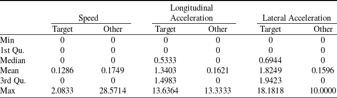
We present the summary statistics of these normalized indices in Table 9. The target trips have higher indices across all three dimensions compared to the other trips, with the differences much more pronounced for both acceleration components. This suggests that the target trips contain more outliers among the trips completed by the same driver, which will facilitate our identification of the target trips. It is important to note that we did not specify the target trips during model training nor pseudo-residuals computation, yet we observe distinct differences in anomaly indices and their normalized versions between the target and all other trips. The right column of Figure 3 displays the empirical density plots of the normalized anomaly indices for the two groups, with target trips represented in red and all other trips in blue.

Figure 3.

Empirical densities of target trips and all other trips for their anomaly indices. The left column shows the raw indices, while the right column shows the normalized indices. Red: target trips, and blue: all other trips.

Table 9.

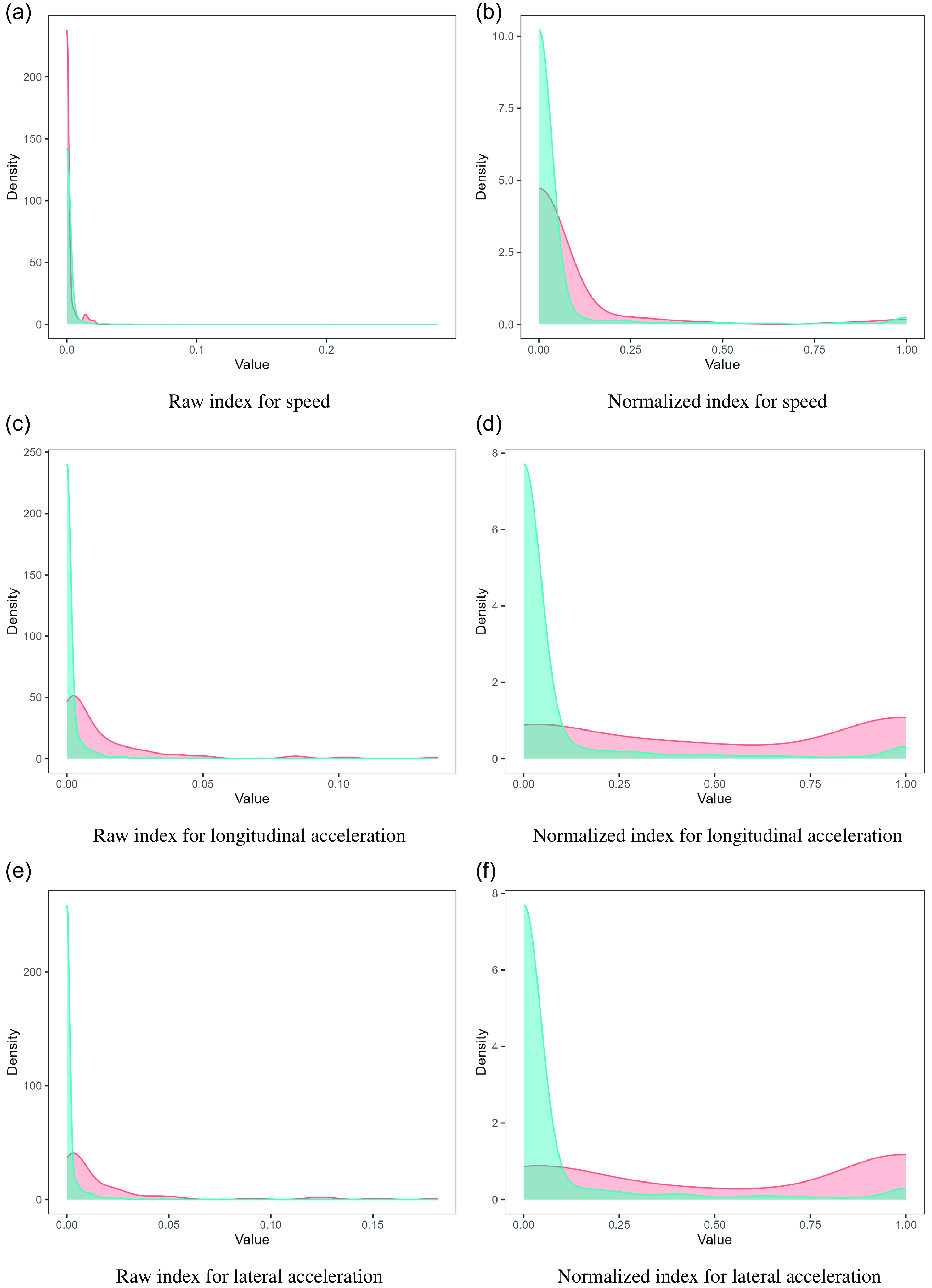
Summary statistics of normalized anomaly indices, computed from CTHMMs with 20 states

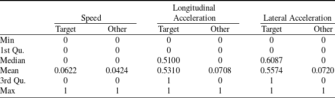
With the three raw or normalized anomaly indices as covariates, we consider three models to predict the probability that a trip is actually a target trip. The candidates are logistic regressions with and without cubic splines (i.e., generalized linear model (GLM) and generalized additive model (GAM), respectively) and XGBoost (eXtreme Gradient Boosting). We implement these models with standard R packages stats, mgcv and xgboost, respectively. For GAM, we specify a cubic regression spline (bs = ‘cr’), while for XGBoost, we use the package’s default parameter settings, adjusting only the number of iteration rounds to 20. This choice ensures reproducibility and consistency, as training log loss stabilizes around 0.001 at this point, indicating sufficient convergence without overfitting. While further optimization of the XGBoost model is possible, our primary focus is on demonstrating the usefulness of the proposed anomaly index in identifying accident-related trips.

We then evaluate model performance based on ROC-AUC (the area under the receiver operating characteristic curve). ROC-AUC is a performance metric frequently used to evaluate the effectiveness for a binary classification model, which quantifies the model’s ability to distinguish between the two classes. A perfect model has an AUC of 1, while a model that randomly guesses has an AUC of 0.5. To robustify the performance evaluation, we perform fivefold cross-validations (CV) for each set of covariates and model. In a k-fold cross validation, the dataset is split into k subsets. In each fold, the model is trained on $k-1$ subsets, and the trained model is tested on the remaining subset. The k-fold CV then reports the average of the k results. Our dataset is randomly partitioned into 5 subsets such that: first, all trips from a window are in the same subset; and second, the proportion of target trips are close (0.05234, 0.05263, 0.05882, 0.05740, and 0.04651).

In Table 10, we report the cross-validation performance of the candidate models with raw or normalized anomaly indices as covariates. We observe that the average ROC-AUCs are all above 0.82, with the ones using normalized indices as covariates performing slightly better for GLM and XGBoost.

Table 10.

Fivefold cross-validation ROC-AUC of logistic models with raw or normalized anomaly indices as covariates.

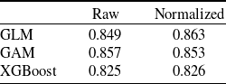
Recall that in practice, the goal is to rank the trips in each 3-day window based on their level of anomalousness, ideally identifying the target trip. To assess the effectiveness of this ranking, we evaluate the ROC-AUC for each 3-day window. In Table 11, we present the mean and median window-based ROC-AUC from cross validation. Furthermore, we report the average accuracy, which we define as the proportion of windows where the ROC-AUC is 1 — that is, when the target trip has the highest predicted probability among trips within the same window and is considered the most anomalous. The results show that models using normalized indices as covariates again perform slightly better on average. Although the average accuracy ranges only between 0.43 and 0.53, achieving a classifier with an AUC of 1 is inherently challenging. This difficulty is amplified in our context, where identifying the target trip requires selecting it from a group that can range from 2 to 63 trips. Nevertheless, it is noteworthy that more than half of the cases achieve perfect classification. Moreover, the relatively high (average) population ROC-AUCs (above 0.82), along with the mean and median window-based ROC-AUCs (above 0.84 and 0.95, respectively), all indicate that the models effectively rank trips by their anomalousness, both overall and within each window, with the target trips often ranked near or at the top.

Table 11.

Fivefold cross-validation window-based ROC-AUC of logistic models with raw or normalized anomaly indices as covariates.

Finally, we fit the models to the whole dataset and report the model summary of GAM in Table 12, while model summary of GLM and feature importance of XGBoost are provided in Appendix C. The findings show that outliers in both longitudinal and lateral accelerations are more significant predictors of target trips than outliers in speed, which is in line with observations from the controlled study.

Table 12.

Model summary of logistic GAMs, with raw or normalized anomaly indices as covariates. Note: x1, x2, and x3 denote indices for speed, longitudinal, and lateral accelerations, respectively.

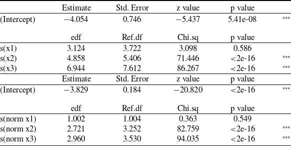
Significance codes: 0 ‘***’, 0.001 ‘**’, 0.01 ‘*’, 0.05 ‘.’, 0.1 ‘ ’, 1

Our proposed CTHMM modelling and anomaly detection framework hold great potential for practical applications, particularly for companies aiming to enhance safety and operational efficiency. For instance, it can be employed to detect anomalous driving behaviours, assess risk factors, and provide actionable feedback to improve driver safety.

In our rental-car dataset, recall that our collaborator’s collision detection method produces accident triggers for only around 10% of claims. By applying the proposed method, we can effectively pinpoint target trips for investigation in the remaining 90% of cases. Moreover, leveraging the analysis of pseudo-residual points, as detailed in Section 5.2, allows us to locate each outlier and delve deeper into its nature. This facilitates the identification of underlying causes, such as harsh braking or cornering events relative to each driver’s driving patterns, and the provision of individualized feedback to mitigate such actions and improve driving practices.

6.3. Pooled model

Lastly, we apply the pooled model to compare trips across individuals and investigate differences in driving behaviour between drivers with and without (at-fault) claims. While we can fit a pooled model using all 35 trips in the controlled study, the sheer number of trips in real-world settings makes it infeasible to train the model on each and every trip. Hence, sampling of trips is necessary for practical model training.

To ensure the robustness of our results, we experiment with multiple training sets. As the claim rate in the dataset is approximately 10%, we decide to create training sets with random stratified samples reflecting this proportion. Each training set consists of 100 rentals, including 10 rentals with at-fault claims and 90 rentals without claims. For the claimed rentals, we consider trips within the 3-day window around the date of loss, while for the no-claim rentals, we consider the 3 days immediately before the rental ends. Additionally, to test the extreme cases, we construct two alternative training sets: one with 0% claim rate (100 no-claim rentals) and one with 100% claim rate (94 rentals with at-fault claims, discussed in Section 6.2), using the same respective 3-day windows.

For our primary analysis, we focus on the 10% claim rate sample, as it aligns with the portfolio average. We train a single 20-state CTHMM with state-dependent distributions gamma for speed and normal for both acceleration components. Training pooled models, such as for 100 rentals, is more computationally intensive than training 100 individual-specific models. This is because each iteration of the EM algorithm must process all trips from the 100 rentals. Based on our experience, fitting such a pooled model takes about a day to complete 5,000 iterations of the EM algorithm. However, once the model is fitted, it can evaluate both existing and newly observed trips.

Using the fitted pooled model, we determine the anomaly indices of all trips from all rentals over their entire rental periods, rather than just a 3-day window. This allows us to examine any differences in driving behaviour, focusing particularly on differences in driving anomalies, between rentals with and without (at-fault) claims. The analysis is repeated with four different random training sets, each with a 10% claim rate, and results are reported in Table 13.

Table 13.

Comparison of anomaly indices (%) in each telematics response dimension for claimed and no-claim rentals, computed from pooled CTHMMs trained on training sets with a 10% claim rate.

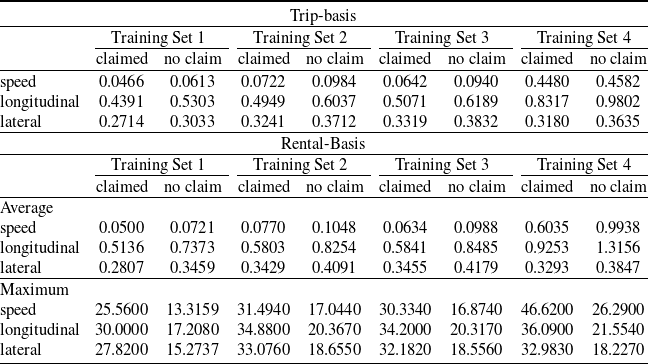
The first question we address is whether there are notable differences in anomaly indices for individual trips performed by the claimed and no-claim groups. In the sub-table titled ‘trip-basis’, we calculate the average indices across all trips completed by each group. We find that the differences are minimal. In fact, the claimed group shows slightly lower average anomaly indices than the no-claim group, which may seem counterintuitive. A plausible explanation is that the model was trained on only 300 days of trip data, which may not capture all major driving behaviour. In contrast, the evaluation spans entire rental periods of over 17,000 rentals, providing a broader context that may dilute the trip-specific differences.

Next, we investigate whether anomaly indices differ when aggregated over entire rental periods for the claimed and no-claim groups. This analysis examines the empirical distribution of anomaly indices for each rental. In the sub-table titled ‘rental-basis’, we present the averages of two metrics for each group: the rental-wise average indices and the rental-wise maximum indices. Specifically, we calculate the average of the rental averages and the average of the rental maximums for each group. While the average indices between the groups remain similar, the claimed group exhibits significantly higher maximums. On average, the maximum indices for the claimed group are roughly double those of the no-claim group across all response dimensions. To help visualize these differences, Figure 4 presents the empirical density plots of the anomaly indices for the claimed and no-claim groups on a rental basis. The left column displays the rental averages, while the right column illustrates the rental maximums, with the claimed group represented in red and the no-claim group in blue.

Figure 4.

Empirical densities of claimed and no-claim groups for their anomaly indices on a rental basis. The left column shows the mean indices over rentals, while the right column shows the maximum over rentals. Red: with claims, and blue: without claims.

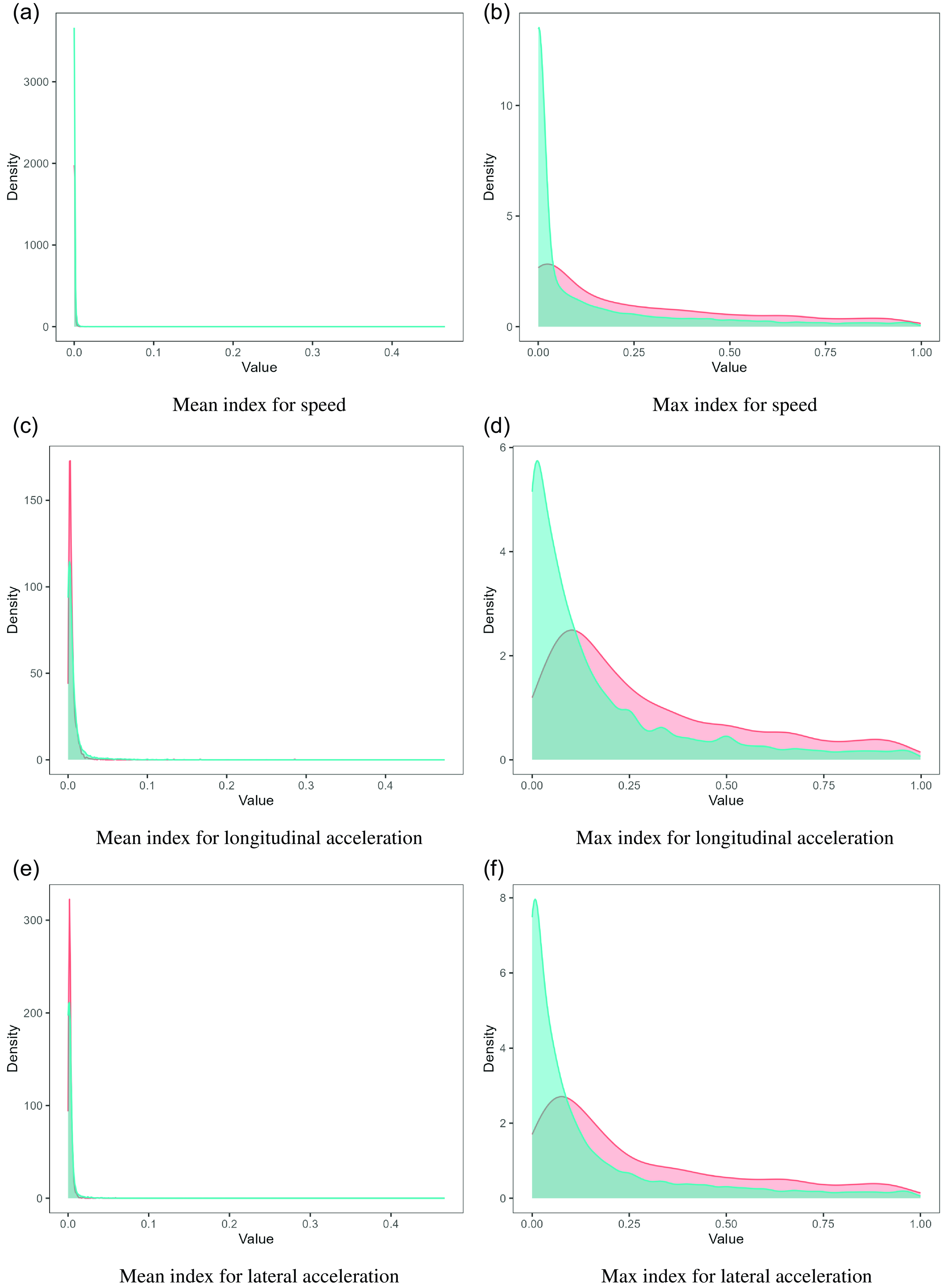
While it may seem counterintuitive that the claimed group has slightly lower average anomaly indices per trip, it is important to recognize that the no-claim group is ten times larger than the claimed group, leading to greater variability in their driving behaviour. This highlights the importance of trip-based risk evaluation, as not every trip by the claimed group is dangerous, and similarly, not all trips by the no-claim group are safe. Over the entire rental period, however, the claimed group consistently exhibits more outliers, with this difference remains significant across all quantiles. This is similar to the finding that higher maximum speed attained is associated with increased driving risk, while average speed is not (Chan et al. (Reference Chan, Tseung, Badescu and Lin2024)). It only takes one very aggressive or anomalous trip to result in an accident and incur a claim.

As mentioned, to further validate the robustness of these findings, we test two alternative training sets with 0% and 100% claim rates, representing two limiting cases. Despite the change in claim rate, the observed trends remain consistent across all scenarios. The claimed group consistently shows slightly lower average trip-based anomaly indices but higher maximum indices across rentals. Additionally, the anomaly indices for longitudinal and lateral acceleration in the claim group are 1.5 to 2 times greater than those in the no-claim group. These persistent observations suggest that the findings are robust and indicative of true underlying behaviour trends. Detailed results from analyses performed with the two alternative training sets (0% and 100% claim rates) are provided in Appendix D.

The next goal of our numerical investigation is to assess the risk associated with each rental. To achieve this, we aim to differentiate between claimed and no-claim rentals and predict the probability of a rental resulting in an at-fault claim. Our analysis relies solely on telematics data, with no additional covariates such as demographic or vehicle-specific information included. Specifically, we consider the following three sets of telematics covariates for predicting the claim probability of each rental:

1. 1. Set 1 includes maximum anomaly indices across all telematics response dimensions;

2. 2. Set 2 includes the right tail of the anomaly index empirical distribution ($\alpha$-th percentiles $P_{\alpha,d}$ for $\alpha=90,\, 95,\, 97,\, 97.5,\, 98,\, 98.5,\, 99,\, 99.5$ and the maximum); and finally

3. 3. Set 3 combines the right tail from Set 2 and the number of trips as an offset (i.e., with regression coefficient 1).

For each covariate set, we fit a logistic regression and evaluate the model performance based on ROC-AUC. To robustify the evaluation, we perform fivefold CV for each set of covariates computed from different pooled CTHMMs (fitted to 4 different training sets). Our dataset is randomly partitioned into 5 subsets with close claim rates (0.1007, 0.0996, 0.0968, 0.0989, and 0.0986).

In Table 14, we report the CV performance. We observe that the average ROC-AUCs are generally stable across anomaly indices computed from pooled CTHMMs trained on different training sets. (Covariate) Set 1 achieves ROC-AUCs around 0.69, while Set 2 improves to 0.74. Since the tail and its smoothness depend on the number of observed data points, we incorporate the exposure, which is the number of trips, as an offset. The resulting ROC-AUCs further improve to around 0.78. We would like to highlight that first, our ROC-AUC values consistently outperform our collaborator’s current benchmark of 0.65, demonstrating the effectiveness of our proposed method; and second, we perform our analysis using solely telematics data, and inclusion of traditional covariates such as driver and vehicle information can definitely further improve the results.

Table 14.

Fivefold cross-validation ROC-AUC of logistic GLMs with different sets of covariates. Set 1: maximum anomaly indices, Set 2: right tail of the anomaly index empirical distribution, Set 3: right tail and the number of trips as an offset.

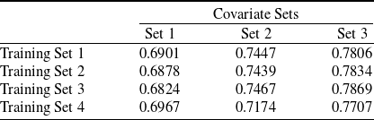
Finally, we fit the logistic GLM to (covariate) Set 3 of the entire portfolio. The model summary is presented in Table 15. In general, larger percentile values of the anomaly indices increase the claim probability. Moreover, the right tails of anomaly index empirical distribution in both longitudinal and lateral accelerations appear to have more significant predictive power for claim probability than that in speed, aligning with our previous findings.

Table 15.

Model summary of logistic GLM with the right tail of the anomaly index empirical distribution and the number of trips as an offset.

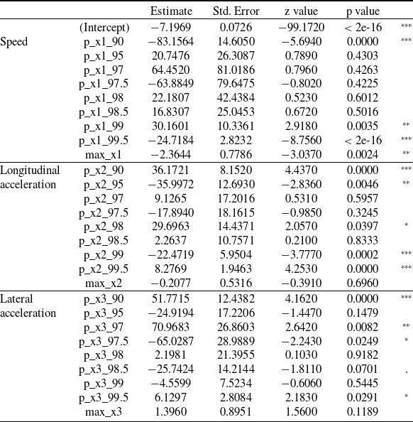
Significance codes: 0 ‘***’, 0.001 ‘**’, 0.01 ‘*’, 0.05 ‘.’, 0.1 ‘ ’, 1