

1 INTRODUCTION
Regression analysis is the cornerstone of statistical theory and practice. Ordinary least squares (OLS) has been applied, within various regression contexts, to build an extensive toolkit, for the exploration of economic and financial datasets. The basic theory underlying OLS estimation and inference in regression models has been largely established for over half of a century (see, e.g., Lai and Wei, Reference Lai and Wei1982). The problem of robust estimation has long been a focus of empirical work in economics, beginning with the seminal work by White (Reference White1980). Its importance is well understood in applied econometrics. At the same time, several important concerns have been raised by applied researchers. Angrist and Pischke (Reference Angrist and Pischke2010) noted that “Leamer (Reference Leamer1983) diagnosed his contemporaries’ empirical work as suffering from a distressing lack of robustness to changes in key assumptions,” and Leamer (Reference Leamer2010) later reflected that “sooner or later, someone articulates the concerns that gnaw away in each of us and asks if the Assumptions are valid.” Similarly, Karmakar, Richter, and Wu (Reference Karmakar, Richter and Wu2022) observed that the assumption of parameter constancy, or “stationarity is often an oversimplified assumption that ignores systematic deviations of parameters from constancy.” Clearly, this concern extends beyond parameter stability to encompass the stability of regressors, regression noise, and the underlying modeling assumptions.
In this article, we focus on the inherent capacity of regression modeling to accommodate the effects of structural change in settings with both fixed and time-varying parameters. Many such structural changes influence not only the model parameters but also the regression space itself. This space comprises both the regressors and regression noise, and improper treatment of these components may result in incorrect inferences, misinterpretations, and forecasting distortions. We therefore examine which specifications of the regression space can flexibly account for structural change while still enabling estimation of both fixed and time-varying regression parameters, the construction of confidence intervals, and the computation of standard errors.
Among recent developments, Wu (Reference Wu2005), Hall, Han, and Boldea (Reference Hall, Han and Boldea2012), and others have proposed advanced theoretical methods for the estimation of the fixed parameters, while Cattaneo, Jansson, and Newey (Reference Cattaneo, Jansson and Newey2018) and Jochmans (Reference Jochmans2019) developed procedures to estimate both fixed parameters and standard errors in regression models with an increasing number of covariates and heteroskedasticity. Meanwhile, Li, Phillips, and Gao (Reference Li, Phillips and Gao2020), Sun et al. (Reference Sun, Hong, Lee, Wang and Zhang2021), and Linton and Xiao (Reference Linton and Xiao2019) introduced new modeling frameworks that explicitly account for structural change. A common response to concerns about heteroskedasticity in the recent literature is the use of the heteroskedasticity-robust variance and standard error estimators for linear regression models (see Eicker, Reference Eicker1963; White, Reference White1980; MacKinnon, Reference MacKinnon, Chen and Swanson2012; Cattaneo et al., Reference Cattaneo, Jansson and Newey2018; among others).
There is also a sizeable and growing literature on the estimation of time-varying coefficient regression models, including the works of Fan and Zhang (Reference Fan and Zhang1999) and Vogt (Reference Vogt2012), among others. This literature further explores tests for different types of parameter variation (see, e.g., Bai and Perron, Reference Bai and Perron1998; Zhang and Wu, Reference Zhang and Wu2012; Zhang and Wu, Reference Zhang and Wu2015; Hu, Kasparis, and Wang, Reference Hu, Kasparis and Wang2025). In addition, specification tests and tests for parameter instability have received significant attention, with important contributions by Hansen (Reference Hansen2000), Georgiev et al. (Reference Georgiev, Harvey, Leybourn and Robert Taylor2018), Hidalgo, Lee, and Seo (Reference Hidalgo, Lee and Seo2019), Boldea, Cornea-Madeira, and Hall (Reference Boldea, Cornea-Madeira and Hall2019), Fu et al. (Reference Fu, Hong, Su and Wang2023), and others.
The modeling of deterministic, smooth parameter evolution has a long history in statistics. Early examples include linear processes with time-varying spectral densities, introduced by Priestley (Reference Priestley1965). This framework is essentially nonparametric and it has been further developed by Robinson (Reference Robinson and Hackl1989), Robinson (Reference Robinson, Hackl and Westland1991), Dahlhaus (Reference Dahlhaus1997), Dahlhaus, Richter, and Wu (Reference Dahlhaus, Richter and Wu2019), and Dahlhaus and Richter (Reference Dahlhaus and Richter2023), some of whom refer to these processes as locally stationary. The estimation of time-varying parameters, as well as fixed parameters under heteroskedasticity in time-series models, has been studied in Dahlhaus and Giraitis (Reference Dahlhaus and Giraitis1998), Xu and Phillips (Reference Xu and Phillips2008), and Dalla, Giraitis, and Robinson (Reference Dalla, Giraitis and Robinson2020), among others. Nonlinear time-varying time-series models have also been developed by Doukhan and Wintenberger (Reference Doukhan and Wintenberger2008), Bardet and Wintenberger (Reference Bardet and Wintenberger2009), Vogt (Reference Vogt2012), and Karmakar et al. (Reference Karmakar, Richter and Wu2022). Despite these advances, such approaches have not been widely adopted in applied economics, where random coefficient models remain more prevalent.
Various methods have been proposed over the years to identify and handle structural change. Early contributions assumed that changes were deterministic, rare, and abrupt. Testing for parameter breaks dates back to the pioneering work by Chow (Reference Chow1960), with further contributions by Brown, Durbin, and Evans (Reference Brown, Durbin and Evans1975) and Ploberger and Krämer (Reference Ploberger and Krämer1992), among others. More recent approaches allow for random evolution of parameters, where changes may be discrete, as in Markov switching models by Hamilton (Reference Hamilton1989) or threshold models by Tong (Reference Tong1990), or continuous as in smooth transition models by Terasvirta (Reference Terasvirta, Ullah and Giles1998), or those driven by unobservable shocks, as in random coefficient models by Nyblom (Reference Nyblom1989). For example, Cogley and Sargent (Reference Cogley and Sargent2005) use random coefficient models to study stochastic volatility, while Primiceri (Reference Primiceri2005) examines whether changes in parameters or in the variance of shocks—policy-induced or otherwise—contributed to the period of macroeconomic calmness known as the “Great Moderation” after 1985. In these frameworks, parameters typically evolve as random walks or autoregressive processes.
Building on this literature, Giraitis, Kapetanios, and Yates (Reference Giraitis, Kapetanios and Yates2014), Giraitis, Taniguchi, and Taqqu (Reference Giraitis, Taniguchi and Taqqu2018), Dendramis, Giraitis, and Kapetanios (Reference Dendramis, Giraitis and Kapetanios2021), and others have developed a theoretical time-series framework for random coefficient models and their estimation using kernel-based methods, which perform well in finite samples. These methods are computationally simple and straightforward to implement in applied research. For example, Chronopoulos, Giraitis, and Kapetanios (Reference Chronopoulos, Giraitis and Kapetanios2022) demonstrated the empirical prevalence of persistent volatility, suggesting that GARCH-type volatility structures may be less common than previously thought. Nevertheless, a full treatment of estimation and inference within a general regression framework has, surprisingly, not yet been provided.
In this article, we provide a rigorous validation of the asymptotic normality of the feasible t-statistic for the estimation of both fixed and time-varying parameters in linear regression models within an extended regression space of regressors and regression disturbances. Our main objective is to describe, in transparent terms, the extended regression space under which such normality is preserved. The class of admissible regressors and regression noises is broad. Regressors are obtained by rescaling and shifting stationary short-memory (SM) sequences, while regression errors are generated by arbitrary rescaling of a stationary martingale difference (m.d.) sequence. The restrictions imposed on the scale factors and mean processes are weak, allowing these to be either deterministic or stochastic, and to vary over time, possibly abruptly or through non-stationary (e.g., unit-root) dynamics. Some assumptions on the scale factors are necessary and resemble the Lindeberg condition in the classical Lindeberg–Feller central limit theorem. Importantly, the robust feasible t-statistic retains the same form and limiting distribution as in the standard setting. The estimator of feasible robust standard errors coincides with the heteroskedasticity-consistent standard error estimator of White (Reference White1980). Our assumptions do not rely on mixing or near-epoch dependence conditions, which commonly prevail throughout the existing literature. Given the generality of the regression space, these assumptions typically require no additional empirical verification.
The estimation framework for fixed regression parameters is developed in Section 2, which introduces the extended regression space, the underlying assumptions, and the main theoretical results. Section 3 establishes the estimation theory for time-varying regression parameters within the same framework. The proofs highlight how the results for the fixed-parameter case naturally extend to the time-varying settings, with only negligible additional terms.
Our results are complementary to existing frameworks. The novelty lies in providing a methodological foundation that confirms the validity of robust regression estimation in an extended regression space. The fundamental theory in this area traces back to Lai and Wei (Reference Lai and Wei1982) who studied regression models with heteroskedastic m.d. noise under eigenvalue-based assumptions. Alternative methods, such as bootstrap procedures, see Hall et al. (Reference Hall, Han and Boldea2012) and Boldea et al. (Reference Boldea, Cornea-Madeira and Hall2019), are widely used in regression analysis but may not be directly applicable to such general class of regressors and regression noises. In contrast, we demonstrate that White-type standard errors remain applicable and computationally straightforward.
All theoretical results are supported by detailed, rigorous proofs. Monte Carlo simulations confirm that the proposed robust regression estimators perform well in finite samples. Overall, the framework developed in this article is particularly suited to modeling economic and financial data, where heterogeneity, structural change, and dependence are inherent features.
The remainder of the article is organized as follows. Section 2 presents the regression setting with the extended regression space, accommodating heterogeneity and dependence, and outlines the theoretical results for infeasible and feasible t-statistics in the case of fixed parameters. Section 3 extends the analysis to time-varying regression parameters. Section 4 addresses regression modeling with missing data patterns. Section 5 illustrates the flexibility of our robust estimation method through its application to the estimation of an AR $(p)$
model generated by a stationary m.d. noise. Section 6 presents Monte Carlo simulation results. In Section 7, we provide an empirical application of the robust regression framework to modeling asset returns. Finally, Section 8 concludes. Proofs and additional simulations are provided in the Supplementary Material.
$(p)$
model generated by a stationary m.d. noise. Section 6 presents Monte Carlo simulation results. In Section 7, we provide an empirical application of the robust regression framework to modeling asset returns. Finally, Section 8 concludes. Proofs and additional simulations are provided in the Supplementary Material.
2 OLS ESTIMATION IN GENERAL REGRESSION SPACE
In this section, we focus on OLS estimation in an environment that permits general heterogeneity in regression modeling. We analyze the model
 $$ \begin{align} y_t=\beta^\prime z_t +u_t, \end{align} $$
where $\beta $
is a p-dimensional parameter vector,
$\beta $
is a p-dimensional parameter vector, $z_t=(z_{1t}, \ldots , z_{pt})^\prime $
is a stochastic regressor, and
$z_t=(z_{1t}, \ldots , z_{pt})^\prime $
is a stochastic regressor, and $u_t$
is an uncorrelated noise term. To include an intercept, the first component can be set as
$u_t$
is an uncorrelated noise term. To include an intercept, the first component can be set as $z_{1t}=1$
. We refer to the collection of
$z_{1t}=1$
. We refer to the collection of $\{z_t, u_t\}$
jointly as “the regression space.”
$\{z_t, u_t\}$
jointly as “the regression space.”
An applied researcher may want to work within a regression space that accommodates a wide range of regressors and regression noises, without being hindered by restrictive technical assumptions. Ideally, such a setting should permit regressors to exhibit non-stationarity and undefined generic structural change, while enabling estimation and inference under weak theoretical constraints that do not require empirical verification.
Our goal is to extend the OLS estimation procedure to a broad regression framework defined by baseline assumptions aligned with empirical research practice. These assumptions cover a wide variety of types of potentially non-stationary regression variables encountered in applied work. The framework achieves a level of generality comparable to that in Giraitis, Li, and Phillips (Reference Giraitis, Li and Phillips2024), which addresses testing for the absence of correlation and cross-correlation under general heterogeneity.
We begin with specifying the structure of an uncorrelated regression noise $u_t$
. Suppose that
$u_t$
. Suppose that
 $$ \begin{align} u_t =h_t\varepsilon_t, \end{align} $$
where $\{\varepsilon _t\}$
is a zero-mean stationary uncorrelated m.d. noise, and
$\{\varepsilon _t\}$
is a zero-mean stationary uncorrelated m.d. noise, and $\{h_t\}$
is a deterministic or stochastic scale factor independent of
$\{h_t\}$
is a deterministic or stochastic scale factor independent of $\{\varepsilon _t\}$
. The following assumption formalizes these conditions.
$\{\varepsilon _t\}$
. The following assumption formalizes these conditions.
Assumption 2.1. $\{\varepsilon _t\}$
is a stationary m.d. noise with respect to some
$\{\varepsilon _t\}$
is a stationary m.d. noise with respect to some $\sigma $
-field filtration
$\sigma $
-field filtration $\mathcal {F}_t $
, such that
$\mathcal {F}_t $
, such that
 $$ \begin{align*} \mathbb{E}[\varepsilon_t|\mathcal{F}_{t-1}]=0,\quad \mathbb{E} \varepsilon_t^8<\infty, \quad \mathbb{E}\varepsilon_t^2=1. \end{align*} $$
The sequence $\{\varepsilon _t\}$
is independent of
$\{\varepsilon _t\}$
is independent of $\{h_t\}$
. Moreover, variable
$\{h_t\}$
. Moreover, variable $ \varepsilon _1$
has a probability density function
$ \varepsilon _1$
has a probability density function $f(x)$
satisfying
$f(x)$
satisfying $f(x)\le c<\infty $
for all
$f(x)\le c<\infty $
for all $|x|\le x_0$
, for some
$|x|\le x_0$
, for some $x_0>0$
and
$x_0>0$
and $c>0$
.
$c>0$
.
The information set $\mathcal {F}_t$
is generated by the past history
$\mathcal {F}_t$
is generated by the past history $\mathcal {F}_t=\sigma (\varepsilon _s, \, s\le t)$
and possibly other variables.
$\mathcal {F}_t=\sigma (\varepsilon _s, \, s\le t)$
and possibly other variables.
A typical example of m.d. noise in applied work is provided by the ARCH/GARCH family and the class of stochastic volatility processes. The specification (2) therefore allows for conditional heteroskedasticity in $u_t$
.
$u_t$
.
We next specify the regressors $z_t=(z_{1t}, \ldots , z_{pt})^\prime $
which form the key structural component of our regression space. For
$z_t=(z_{1t}, \ldots , z_{pt})^\prime $
which form the key structural component of our regression space. For $k=1, \ldots , p$
, the regressors can be written as
$k=1, \ldots , p$
, the regressors can be written as
 $$ \begin{align} z_{kt}=\mu_{kt}+g_{kt}\eta_{kt},\quad t=1, \ldots, n, \end{align} $$
where $\eta _t=(\eta _{1t}, \ldots , \eta _{pt})^\prime $
is a stationary sequence,
$\eta _t=(\eta _{1t}, \ldots , \eta _{pt})^\prime $
is a stationary sequence, $ g_t=(g_{1t},\ldots , g_{pt})^\prime $
are deterministic or stochastic scale factors, and
$ g_t=(g_{1t},\ldots , g_{pt})^\prime $
are deterministic or stochastic scale factors, and $\mu _t=(\mu _{1t}, \ldots , \mu _{pt})^\prime $
is a vector of deterministic or stochastic means. We assume that
$\mu _t=(\mu _{1t}, \ldots , \mu _{pt})^\prime $
is a vector of deterministic or stochastic means. We assume that $\{\mu _t, g_t,h_t\}$
are independent of
$\{\mu _t, g_t,h_t\}$
are independent of $\{\varepsilon _t, \,\eta _t\}$
. To include an intercept in model (1), we set
$\{\varepsilon _t, \,\eta _t\}$
. To include an intercept in model (1), we set
 $$ \begin{align} z_{1t}\equiv 1= \mu_{1t}+g_{1t}\eta_{1t}, \quad \mu_{1t}=0, \quad g_{1t}=\eta_{1t}=1. \end{align} $$
We further suppose that in (3) $E\eta _{kt}=0$
except for the intercept (4), where
$E\eta _{kt}=0$
except for the intercept (4), where $\eta _{1t}=1$
.
$\eta _{1t}=1$
.
In summary, the admissible regressors $\{z_t\}$
in our setting are obtained by shifting and rescaling an SM stationary process
$\{z_t\}$
in our setting are obtained by shifting and rescaling an SM stationary process $\{\eta _t\}$
by the mean process
$\{\eta _t\}$
by the mean process $\mu _t$
and the scale factor
$\mu _t$
and the scale factor $ g_t$
:
$ g_t$
:
 $$ \begin{align*}z_t=\mu_t+I_{gt}\eta_t, \quad I_{gt}= \mathrm{diag}(g_{1t}, \ldots, g_{pt}). \end{align*} $$
The underlying stationary sequence $\{\eta _t\}$
is the fundamental component structuring regressors
$\{\eta _t\}$
is the fundamental component structuring regressors $z_t$
. Estimation of the regression parameter
$z_t$
. Estimation of the regression parameter $\beta $
requires only mild assumptions on
$\beta $
requires only mild assumptions on $\{\mu _t,g_t\}$
, and SM dependence assumption on
$\{\mu _t,g_t\}$
, and SM dependence assumption on $\eta _t$
, satisfied by ARMA and related stationary time-series models. This framework eliminates the need for additional empirical validation.
$\eta _t$
, satisfied by ARMA and related stationary time-series models. This framework eliminates the need for additional empirical validation.
Definition 2.1. A (univariate) covariance stationary sequence $\{\xi _t\}$
has short-memory (SM) if
$\{\xi _t\}$
has short-memory (SM) if $\sum _{h=-\infty }^\infty | \mathrm {cov}(\xi _h,\xi _0)|<\infty. $
Assumption 2.2. $\eta _t=(\eta _{1t}, \ldots , \eta _{pt})^\prime $
is an
$\eta _t=(\eta _{1t}, \ldots , \eta _{pt})^\prime $
is an $\mathcal {F} _{t-1}$
-measurable sequence with
$\mathcal {F} _{t-1}$
-measurable sequence with $E[\eta _{kt}^2]=1$
and
$E[\eta _{kt}^2]=1$
and $E[\eta _{kt}^8]<\infty $
.
$E[\eta _{kt}^8]<\infty $
.
(i) For $k,j=1, \ldots , p$
, the sequences
$k,j=1, \ldots , p$
, the sequences $\{\eta _{kt}\}$
and
$\{\eta _{kt}\}$
and $ \{\eta _{jt}\eta _{kt}\}$
are covariance stationary and have SM.
$ \{\eta _{jt}\eta _{kt}\}$
are covariance stationary and have SM.
(ii) The matrix $E[\eta _1\eta _1^\prime ]$
is positive definite.
$E[\eta _1\eta _1^\prime ]$
is positive definite.
The novelty of this regression framework lies in the structural specification (3), which accommodates regressors $z_t=(z_{1t}, \ldots , z_{pt})^\prime $
that may be deterministic or stochastic, and stationary or non-stationary. This flexibility arises from allowing a broad class of scale factors and mean processes
$z_t=(z_{1t}, \ldots , z_{pt})^\prime $
that may be deterministic or stochastic, and stationary or non-stationary. This flexibility arises from allowing a broad class of scale factors and mean processes $\{h_t, g_t, \mu _t\}$
which brings the OLS estimation closer to empirical practice.
$\{h_t, g_t, \mu _t\}$
which brings the OLS estimation closer to empirical practice.
The estimation framework also accommodates triangular arrays of means and scale factors: $\big (\mu _t, g_{t}, h_{t},\,\,\, t=1,\ldots , n\big )=\big (\mu _{nt}, g_{nt}, h_{nt}, \,\,\,t=1,\ldots , n\big )$
. Throughout the article, we assume that these quantities may depend on the sample size n. For brevity of notation, the subscript n is omitted.
$\big (\mu _t, g_{t}, h_{t},\,\,\, t=1,\ldots , n\big )=\big (\mu _{nt}, g_{nt}, h_{nt}, \,\,\,t=1,\ldots , n\big )$
. Throughout the article, we assume that these quantities may depend on the sample size n. For brevity of notation, the subscript n is omitted.
The underlying stationary noise component $\eta _t$
in the regressors
$\eta _t$
in the regressors $z_t$
in (3) is weakly exogenous with respect to the stationary m.d. noise
$z_t$
in (3) is weakly exogenous with respect to the stationary m.d. noise $\varepsilon _t$
in
$\varepsilon _t$
in $u_t = h_t \varepsilon _t$
. The mean and scale factors
$u_t = h_t \varepsilon _t$
. The mean and scale factors $\{\mu _t,g_t\}$
are independent of
$\{\mu _t,g_t\}$
are independent of $\{\varepsilon _t\}$
, though they may be dependent on
$\{\varepsilon _t\}$
, though they may be dependent on $\{h_t\}$
. Overall,
$\{h_t\}$
. Overall, $\{\mu _t, g_t, h_t\}$
are mutually independent of
$\{\mu _t, g_t, h_t\}$
are mutually independent of $\{\eta _t, \varepsilon _t\}$
, while potential dependence among
$\{\eta _t, \varepsilon _t\}$
, while potential dependence among $\{\mu _t\}$
,
$\{\mu _t\}$
, $\{g_t\},$
and
$\{g_t\},$
and $\{h_t\}$
, and their components, is unrestricted.
$\{h_t\}$
, and their components, is unrestricted.
The processes $\mu _{kt}$
and
$\mu _{kt}$
and $g_{kt}$
can be interpreted as conditional mean and variance,
$g_{kt}$
can be interpreted as conditional mean and variance, $\mu _{kt}=E[z_{kt}\, |\mathcal {F}_n^*]$
, and
$\mu _{kt}=E[z_{kt}\, |\mathcal {F}_n^*]$
, and $g_{kt}^2=\mathrm {var}(z_{kt}|\mathcal {F}_n^*) $
of
$g_{kt}^2=\mathrm {var}(z_{kt}|\mathcal {F}_n^*) $
of $z_{kt}$
, where
$z_{kt}$
, where $\mathcal {F}_n^*=\sigma \big (\mu _t, g_t,h_t, t=1, \ldots , n\big )$
denotes the information set generated by the means and scale factors.
$\mathcal {F}_n^*=\sigma \big (\mu _t, g_t,h_t, t=1, \ldots , n\big )$
denotes the information set generated by the means and scale factors.
Denote for $k=1, \ldots , p$
,
$k=1, \ldots , p$
,
 $$ \begin{align} v_k^2&=\sum_{t=1}^n g_{kt}^2h_t^2,\quad v_{gk}^2=\sum_{t=1}^n g_{kt}^2,\\ D&=\mathrm{diag}(v_1,\ldots, v_p), \quad D_g=\mathrm{diag}(v_{g1},\ldots, v_{gp}).\nonumber \end{align} $$
We write $a_n\asymp _p b_n$
if
$a_n\asymp _p b_n$
if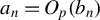 $a_n=O_p(b_n)$
and
$a_n=O_p(b_n)$
and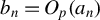 $b_n=O_p(a_n)$
.
$b_n=O_p(a_n)$
.
Assumption 2.3. The scale factors $h_t\ge 0$
and
$h_t\ge 0$
and $g_t\ge 0$
are deterministic or stochastic non-negative variables such that, for
$g_t\ge 0$
are deterministic or stochastic non-negative variables such that, for $k=1, \ldots , p$
,
$k=1, \ldots , p$
,
 $$ \begin{align} &\frac{\max_{1\le t \le n}g_{kt}^2}{v_{gk}^2}= o_p(1),\quad \frac{ \max_{1\le t \le n}\mu_{kt}^2}{v_{gk}^2}= o_p(1), \end{align} $$
 $$ \begin{align} &\frac{\sum_{t=1}^n \mu_{kt}^2}{v_{gk}^2}= O_p(1),\quad \frac{\sum_{t=1}^n \mu_{kt}^2h_t^2}{v_{k}^2}= O_p(1), \quad v_k^2\asymp_pv^2_{gk}, \quad v_k \rightarrow_p\infty. \end{align} $$
Assumptions (6) and (7) impose only mild restrictions on the means $\mu _t$
and scale factors
$\mu _t$
and scale factors $g_t$
. In particular, condition (6) resembles the Lindeberg condition in the classical Lindeberg–Feller central limit theorem, as it excludes the possibility that the OLS estimation is dominated by a single extreme observation of
$g_t$
. In particular, condition (6) resembles the Lindeberg condition in the classical Lindeberg–Feller central limit theorem, as it excludes the possibility that the OLS estimation is dominated by a single extreme observation of $z_t$
.
$z_t$
.
The first restriction on $g_{kt}$
in (6) is necessary. For example, consider the regressor
$g_{kt}$
in (6) is necessary. For example, consider the regressor $z_t=g_{t}\eta _{t}, t=1, \ldots , n$
, with scale factors
$z_t=g_{t}\eta _{t}, t=1, \ldots , n$
, with scale factors $g_{1}=1$
and
$g_{1}=1$
and $g_{2}=g_{3}=\cdots =g_{n}=0$
, so that
$g_{2}=g_{3}=\cdots =g_{n}=0$
, so that $z_{2}=z_{3}=\cdots =z_{n}=0$
. In this case, the OLS estimator of
$z_{2}=z_{3}=\cdots =z_{n}=0$
. In this case, the OLS estimator of $\beta $
is inconsistent, and such a scale factor
$\beta $
is inconsistent, and such a scale factor $g_t$
does not satisfy (6).
$g_t$
does not satisfy (6).
The second condition (7) ensures that OLS estimation is driven by the stochastic component $g_t\eta _t$
of the regressor
$g_t\eta _t$
of the regressor $z_t$
, rather than by a deterministic or stochastic drift in
$z_t$
, rather than by a deterministic or stochastic drift in $\mu _t$
. In the presence of an intercept, condition (7) further implies that
$\mu _t$
. In the presence of an intercept, condition (7) further implies that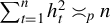 $\sum _{t=1}^n h_t^2\asymp _pn$
, since
$\sum _{t=1}^n h_t^2\asymp _pn$
, since $v_1^2\asymp _pv^2_{g1}$
,
$v_1^2\asymp _pv^2_{g1}$
, $g_{1t}=1$
,
$g_{1t}=1$
, $v_{g1}^2=n$
, and
$v_{g1}^2=n$
, and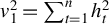 $v_{1}^2=\sum _{t=1}^n h_t^2$
.
$v_{1}^2=\sum _{t=1}^n h_t^2$
.
To estimate $\beta =(\beta _1, \ldots , \beta _p)^\prime $
, we use the standard OLS estimator
$\beta =(\beta _1, \ldots , \beta _p)^\prime $
, we use the standard OLS estimator
 $$ \begin{align} \widehat \beta=\Bigg( \sum_{j=1}^n z_j z_j^\prime\Bigg)^{-1}\Bigg( \sum_{j=1}^n z_j y_j\Bigg) \end{align} $$
computed from the sample $y_j, z_j, \,j=1, \ldots , n$
.
$y_j, z_j, \,j=1, \ldots , n$
.
Consistency: We first establish the consistency of the OLS estimator $\widehat \beta $
.
$\widehat \beta $
.
Theorem 2.1. Suppose that $(y_1, \ldots , y_n)$
is a sample from the regression model (1) and Assumptions 2.1–2.3 are satisfied. Then, the OLS estimator
$(y_1, \ldots , y_n)$
is a sample from the regression model (1) and Assumptions 2.1–2.3 are satisfied. Then, the OLS estimator $\widehat \beta $
is consistent, that is,
$\widehat \beta $
is consistent, that is,
 $$ \begin{align} D( \widehat \beta -\beta) = \big(v_1(\widehat \beta_1 -\beta_1),\ldots,v_p(\widehat \beta_p -\beta_p)\big)^\prime=O_p(1). \end{align} $$
This result implies that the k-th component $\widehat \beta _k$
of the OLS estimator is
$\widehat \beta _k$
of the OLS estimator is $v_k$
-consistent, that is,
$v_k$
-consistent, that is, $\widehat \beta _k -\beta _k = O_p(v_k^{-1})$
. The convergence rate
$\widehat \beta _k -\beta _k = O_p(v_k^{-1})$
. The convergence rate $v_k$
may deviate from the conventional
$v_k$
may deviate from the conventional $\sqrt {n}$
rate and may differ across components. From the definition of
$\sqrt {n}$
rate and may differ across components. From the definition of $v_k$
and
$v_k$
and $v_{gk}$
, it follows that
$v_{gk}$
, it follows that
 $$ \begin{align} \text{if } g_{kt},h_t\ge c>0 \text{ for all } t,n, \text{ then } v_k, v_{gk}\ge c\sqrt n. \end{align} $$
Asymptotic Normality: The asymptotic normality of an element $\widehat \beta _k$
of the OLS estimator, as well as the computation of its standard errors, requires additional assumptions on the scale factors and the stationary processes
$\widehat \beta _k$
of the OLS estimator, as well as the computation of its standard errors, requires additional assumptions on the scale factors and the stationary processes $\{\eta _t, \varepsilon _t\}$
.
$\{\eta _t, \varepsilon _t\}$
.
Assumption 2.4. (i) For $k,j=1, \ldots , p$
, the sequences
$k,j=1, \ldots , p$
, the sequences $\{\varepsilon _t^2\}$
,
$\{\varepsilon _t^2\}$
, $\{\eta _{jt}\varepsilon _t^2\},$
and
$\{\eta _{jt}\varepsilon _t^2\},$
and $\{\eta _{jt}\eta _{kt}\varepsilon _t^2\}$
are covariance stationary and have SM. (ii) For
$\{\eta _{jt}\eta _{kt}\varepsilon _t^2\}$
are covariance stationary and have SM. (ii) For $k=1, \ldots , p,$
 $$ \begin{align} \frac{\max_{1\le t \le n}g_{kt}^2h_t^2}{v_{k}^2}= o_p(1),\quad \frac{ \max_{1\le t \le n}\mu_{kt}^2h_t^2}{v_{k}^2}= o_p(1). \end{align} $$
Assumption 2.4(i) is not required when $\varepsilon _t$
is i.i.d. Together, Assumptions 2.3 and 2.4(ii) exclude cases in which the mean process
$\varepsilon _t$
is i.i.d. Together, Assumptions 2.3 and 2.4(ii) exclude cases in which the mean process $\mu _t$
or a few extreme observations of
$\mu _t$
or a few extreme observations of $z_t$
or
$z_t$
or $u_t$
dominate the estimation of the regression parameter. Overall, these assumptions are mild. They accommodate both deterministic and stochastic means
$u_t$
dominate the estimation of the regression parameter. Overall, these assumptions are mild. They accommodate both deterministic and stochastic means $\mu _t$
and scale factors
$\mu _t$
and scale factors $h_t, g_{t}$
that may change abruptly over time unlike other theoretically rigorous treatments, which restrict structural change to be deterministic and smooth. This flexibility makes the framework particularly suitable for modeling financial data, as it allows for volatility jumps, commonly observed in empirical finance (see, e.g., Eraker, Johannes, and Polson, Reference Eraker, Johannes and Polson2003). In modern macroeconomic VAR models, the scale factor
$h_t, g_{t}$
that may change abruptly over time unlike other theoretically rigorous treatments, which restrict structural change to be deterministic and smooth. This flexibility makes the framework particularly suitable for modeling financial data, as it allows for volatility jumps, commonly observed in empirical finance (see, e.g., Eraker, Johannes, and Polson, Reference Eraker, Johannes and Polson2003). In modern macroeconomic VAR models, the scale factor $h_t$
in the uncorrelated noise representation
$h_t$
in the uncorrelated noise representation $u_t=h_t\varepsilon _t$
is typically assumed to be stochastic (see, e.g., Chan, Koop, and Xuewen, Reference Chan, Koop and Xuewen2024; Carriero et al., Reference Carriero, Clark, Marcellino and Mertens2024), which our framework naturally encompasses.
$u_t=h_t\varepsilon _t$
is typically assumed to be stochastic (see, e.g., Chan, Koop, and Xuewen, Reference Chan, Koop and Xuewen2024; Carriero et al., Reference Carriero, Clark, Marcellino and Mertens2024), which our framework naturally encompasses.
Lemma 2.1 below shows that Assumptions 2.3 and 2.4(ii) hold for regressors $z_t$
and noises
$z_t$
and noises $u_t$
with bounded
$u_t$
with bounded $4+\delta $
moments satisfying (10). The following example provides additional sufficient conditions.
$4+\delta $
moments satisfying (10). The following example provides additional sufficient conditions.
Example 2.1. Assumptions 2.3 and 2.4(ii) are satisfied by regressors $z_t$
and noise
$z_t$
and noise $u_t$
whose scale factors
$u_t$
whose scale factors $h_t,g_t$
and means
$h_t,g_t$
and means $\mu _t$
satisfy
$\mu _t$
satisfy $0<c\le h_t, g_{kt}\le C, \,\,\, ||\mu _t||\le C,$
where
$0<c\le h_t, g_{kt}\le C, \,\,\, ||\mu _t||\le C,$
where $0<c,\,C<\infty $
do not depend on
$0<c,\,C<\infty $
do not depend on $t, n$
or
$t, n$
or $k=1, \ldots , p$
.
$k=1, \ldots , p$
.
When $0<c\le h_t\le C$
,
$0<c\le h_t\le C$
, $||\mu _t||\le C$
for all
$||\mu _t||\le C$
for all $t, n$
, Assumptions 2.3 and 2.4(ii) hold for scale factors
$t, n$
, Assumptions 2.3 and 2.4(ii) hold for scale factors $g_{kt}$
satisfying
$g_{kt}$
satisfying
 $$ \begin{align*} \frac{\min_{t=1, \ldots, n}g^2_{kt}}{\sum_{t=1}^ng^2_{kt}}=o_p(1), \quad k=1, \ldots, p. \end{align*} $$
This condition is, for example, met when $g_{kt}$
follows a unit root process defined by
$g_{kt}$
follows a unit root process defined by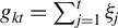 $g_{kt}=\sum _{j=1}^t \xi _j$
, where
$g_{kt}=\sum _{j=1}^t \xi _j$
, where $\{\xi _j$
} is a sequence of i.i.d.
$\{\xi _j$
} is a sequence of i.i.d. $(0, \sigma ^2)$
random variables with finite moments of order
$(0, \sigma ^2)$
random variables with finite moments of order $\theta>2$
. The idea of modeling parameters as unit root processes was discussed, for example, in Nyblom (Reference Nyblom1989).
$\theta>2$
. The idea of modeling parameters as unit root processes was discussed, for example, in Nyblom (Reference Nyblom1989).
We now describe infeasible standard errors $\sqrt {\omega _{kk}}$
using the notation:
$\sqrt {\omega _{kk}}$
using the notation:
 $$ \begin{align} &{S_{zz}=\sum_{t=1}^n z_tz^\prime_t, \quad S_{zzuu}=\sum_{t=1}^n z_tz^\prime_t u_t^2,} \notag \\ &\Omega_n=E[S_{zz} \,|\mathcal{F}^*_n]^{-1}E[S_{zzuu}\,|\mathcal{F} ^*_n]E[S_{zz}\,|\mathcal{F}^*_n]^{-1}=(\omega_{jk}), \end{align} $$
where $\omega _{jk}$
denotes the
$\omega _{jk}$
denotes the $(j,k)$
-th element of the matrix
$(j,k)$
-th element of the matrix $\Omega _n$
. The infeasible standard error of
$\Omega _n$
. The infeasible standard error of $\widehat \beta _k$
is defined as
$\widehat \beta _k$
is defined as $\sqrt {\omega _{kk}}$
, that is, the square root of the corresponding diagonal element of
$\sqrt {\omega _{kk}}$
, that is, the square root of the corresponding diagonal element of $\Omega _n$
.
$\Omega _n$
.
The generality of our regression setting limits the multivariate asymptotic theory that can be established for $ \widehat \beta$
. While a full joint distribution of
$ \widehat \beta$
. While a full joint distribution of $ \widehat \beta$
is not available, we can derive asymptotic normality for linear combinations
$ \widehat \beta$
is not available, we can derive asymptotic normality for linear combinations $a^\prime \widehat \beta $
and then construct feasible inference for the individual component
$a^\prime \widehat \beta $
and then construct feasible inference for the individual component $ \beta _k$
.
$ \beta _k$
.
Existing literature typically imposes stronger assumptions on regressors and errors, such as mixing regressors (White, Reference White2014, Thm. 3.78), locally stationary regressors in Zhang and Wu (Reference Zhang and Wu2012, Eqn. (2.3)), or near-epoch-dependent errors in (Hall et al., Reference Hall, Han and Boldea2012, Assumption 8).
Theorem 2.2. Suppose that the assumptions of Theorem 2.1 and Assumption 2.4 hold. Then, for any $a=(a_1, \ldots , a_p)^\prime \ne 0 $
, the OLS estimator
$a=(a_1, \ldots , a_p)^\prime \ne 0 $
, the OLS estimator $\widehat \beta $
satisfies
$\widehat \beta $
satisfies
 $$ \begin{align} \frac{a^\prime D( \widehat \beta -\beta)}{\sqrt{a^\prime D\Omega_n D a }} \rightarrow _d \mathcal{N}(0, 1). \end{align} $$
In particular, for $k=1, \ldots , p$
, the t-statistic for
$k=1, \ldots , p$
, the t-statistic for $\beta _k$
satisfies
$\beta _k$
satisfies
 $$ \begin{align} \frac{\widehat \beta_k -\beta_k}{\sqrt{\omega_{kk}}}\rightarrow _d \mathcal{N }(0, 1). \end{align} $$
Property (13) is difficult to implement in practice because it requires estimation of the unknown matrices $D,\, \Omega _n$
, except in the special case
$D,\, \Omega _n$
, except in the special case $a^\prime =(0, \ldots ,1,\ldots ,0)$
with only the k-th element being nonzero. In this case, (13) reduces to (14), and the infeasible standard error
$a^\prime =(0, \ldots ,1,\ldots ,0)$
with only the k-th element being nonzero. In this case, (13) reduces to (14), and the infeasible standard error $ \sqrt {\omega _{kk}}$
can be consistently estimated by
$ \sqrt {\omega _{kk}}$
can be consistently estimated by
 $$ \begin{align} \widehat \Omega_n=S_{zz}^{-1}S_{zz\widehat u \widehat u}S_{zz}^{-1}=(\widehat \omega_{jk}), \quad \widehat u_t=y_t-\widehat \beta^\prime z_t. \end{align} $$
The feasible standard error $\sqrt {\widehat \omega _{kk}}$
is the square root of the diagonal element
$\sqrt {\widehat \omega _{kk}}$
is the square root of the diagonal element $\widehat \omega _{kk}$
of
$\widehat \omega _{kk}$
of $\widehat \Omega _n$
.
$\widehat \Omega _n$
.
Corollary 2.1. Under the assumptions of Theorem 2.2, for $k=1, \ldots , p$
, as
$k=1, \ldots , p$
, as $n \rightarrow \infty $
,
$n \rightarrow \infty $
,
 $$ \begin{align} \frac{\widehat \beta_k -\beta_k}{\sqrt{\widehat \omega_{kk}}}\rightarrow _d \mathcal{N}(0, 1), \quad \frac{\widehat \omega_{kk}}{ \omega_{kk}} =1+o_p(1),\quad \sqrt{ \omega_{kk}}\asymp_pv_k^{-1}. \end{align} $$
This result is the main contribution of Section 2. It enables straightforward computation of standard errors and the construction of confidence intervals for $\beta _k$
in the extended regression framework. Notably, the estimator
$\beta _k$
in the extended regression framework. Notably, the estimator $\widehat \Omega _n$
coincides with the heteroskedasticity-consistent standard error estimator of White (Reference White1980).
$\widehat \Omega _n$
coincides with the heteroskedasticity-consistent standard error estimator of White (Reference White1980).
Remark 2.1. The consistency rate $v_k =(\sum _{t=1}^n g_{kt}^2 h_t^2)^{1/2}$
for the parameter
$v_k =(\sum _{t=1}^n g_{kt}^2 h_t^2)^{1/2}$
for the parameter $\beta _k$
may take the form
$\beta _k$
may take the form $v_k\sim c n^\alpha $
for any
$v_k\sim c n^\alpha $
for any $\alpha>0$
, ranging from a super-slow
$\alpha>0$
, ranging from a super-slow $(0<\alpha <1)$
to a super-fast
$(0<\alpha <1)$
to a super-fast $(\alpha>1)$
convergence. To illustrate this, consider the regression model
$(\alpha>1)$
convergence. To illustrate this, consider the regression model
 $$ \begin{align*} y_t&=\beta_1+\beta_2 z_{2t}+\beta_3 z_{3t}+u_t,\quad u_t=h_t\varepsilon_t \text{ with } h_t=1,\\ & z_{kt}=g_{kt}\eta_{kt}, \quad g_{kt} =t^{(\alpha_k-1)/2} \,\, \text{for } k=2,3, \end{align*} $$
where $\alpha _2>1$
,
$\alpha _2>1$
, $0<\alpha _3<1$
, and
$0<\alpha _3<1$
, and $\{\eta _{2t}\}$
,
$\{\eta _{2t}\}$
, $\{\eta _{3t}\}$
,
$\{\eta _{3t}\}$
, $\{\varepsilon _t\}$
are i.i.d.
$\{\varepsilon _t\}$
are i.i.d. ${\cal N}(0,1)$
. Then
${\cal N}(0,1)$
. Then $v_1=\sqrt n$
and
$v_1=\sqrt n$
and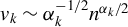 $v_k\sim \alpha _k^{-1/2}n^{\alpha _k/2}$
for
$v_k\sim \alpha _k^{-1/2}n^{\alpha _k/2}$
for $k=2,3$
, producing different convergence rates across the parameters. Even in this simple case, the usual multivariate asymptotic normality for
$k=2,3$
, producing different convergence rates across the parameters. Even in this simple case, the usual multivariate asymptotic normality for $\sqrt n(\widehat \beta -\beta )$
does not hold.
$\sqrt n(\widehat \beta -\beta )$
does not hold.
Corollary 2.1 allows us to establish the asymptotic power and consistency of the test for testing the hypothesis
 $$\begin{align*}H_0: \beta_k = \beta_k^0, \quad \mathrm{vs.} \quad H_1: \beta_k \ne \beta_k^0, \end{align*}$$
that is, whether the k-th element of the regression parameter $\beta =(\beta _1,\ldots ,\beta _p)^\prime $
is equal to a specific value
$\beta =(\beta _1,\ldots ,\beta _p)^\prime $
is equal to a specific value $\beta _k^0$
.
$\beta _k^0$
.
Corollary 2.2. Suppose that $\beta _k^0 \ne \beta _k$
. Then, under the assumptions of Corollary 2.1,
$\beta _k^0 \ne \beta _k$
. Then, under the assumptions of Corollary 2.1,
 $$ \begin{align} t = \frac{\widehat \beta_k - \beta_k^0}{\sqrt{\widehat \omega_{kk}}} \ \asymp_p \ v_k \ \rightarrow_p \ \infty. \end{align} $$
We conclude this section with a lemma that provides simple sufficient moment-type conditions for the validity of Assumptions 2.3 and 2.4(ii). In particular, condition (10) implies (19).
Lemma 2.1. Suppose that for $k=1, \ldots , p$
,
$k=1, \ldots , p$
,
 $$ \begin{align} Ez_{kt}^4\le c,\quad E|u_t|^{4+\delta}\le c \,\,\,\, \text{for some } \delta>0, \end{align} $$
 $$ \begin{align} n/v_k^2&=O_p(1), \quad n/v_{gk}^2=O_p(1), \end{align} $$
where $c<\infty $
does not depend on
$c<\infty $
does not depend on $t,n$
. Then Assumptions 2.3 and 2.4(ii) hold.
$t,n$
. Then Assumptions 2.3 and 2.4(ii) hold.
In particular, (19) is satisfied if $\max _{t=1, \ldots , n}h_t^{-1}=O_p(1)$
and
$\max _{t=1, \ldots , n}h_t^{-1}=O_p(1)$
and $\max _{t=1, \ldots , n}g_{kt}^{-1}=O_p(1).$
The regular estimator of standard errors in OLS regression estimation is given by
 $$ \begin{align} \widehat \Omega_{n}^{(st)}=S_{zz}^{-1} \,\widehat \sigma ^2_u, \quad \widehat \sigma ^2_u=n^{-1}\sum_{j=1}^n\widehat u_j^2. \end{align} $$
Unlike the robust standard errors $\sqrt {\widehat \omega _{kk}}$
, these conventional standard errors may produce coverage distortions, particularly when heteroskedasticity or heterogeneity in
$\sqrt {\widehat \omega _{kk}}$
, these conventional standard errors may produce coverage distortions, particularly when heteroskedasticity or heterogeneity in $g_t$
,
$g_t$
, $h_t$
, or
$h_t$
, or $\mu _t$
is present (see Section 6). This underscores the robustness and strong empirical relevance of the normal approximation in (16).
$\mu _t$
is present (see Section 6). This underscores the robustness and strong empirical relevance of the normal approximation in (16).
This section validates the asymptotic normality of the feasible t-statistics for the components of the OLS estimator in linear regression models with general heterogeneity. The assumptions imposed are mild yet flexible, allowing a wide class of (possibly nonstationary) regressors and noise processes beyond those typically considered in the existing literature. Some conditions on scale factors are analogous to the Lindeberg condition and remain necessary. Our framework complements, rather than replaces, prior approaches; for instance, near-unit-root regressors in Georgiev et al. (Reference Georgiev, Harvey, Leybourn and Robert Taylor2018) require a distinct theoretical treatment. Although bootstrap methods, see, for example, Hall et al. (Reference Hall, Han and Boldea2012) and Boldea et al. (Reference Boldea, Cornea-Madeira and Hall2019), are widely applied in regression analysis, they may not extend to the heterogeneous structures considered here. By contrast, we demonstrate that the heteroskedasticity-consistent standard errors of White (Reference White1980) remain applicable and computationally straightforward.
Our focus in this article is model (1), where the regression noise $u_t$
in (1) is uncorrelated. Extending the asymptotic theory to account for dependence in
$u_t$
in (1) is uncorrelated. Extending the asymptotic theory to account for dependence in $u_t$
is a natural next step and is currently under consideration.
$u_t$
is a natural next step and is currently under consideration.
Proofs of all results are provided in the Supplementary Material.
3 TIME-VARYING OLS ESTIMATION IN THE EXTENDED REGRESSION SPACE
This section demonstrates further advantages of the theory of regression estimation with a fixed parameter, developed in Section 2. Thanks to the flexible setting, the estimation of time-varying parameters naturally follows from our theory for fixed-parameter regression in the extended space, along with bounding of some negligible terms.
In the previous section, we discussed the estimation of regression model (1), $y_j=\beta ^\prime z_j +u_j$
, with a fixed parameter
$y_j=\beta ^\prime z_j +u_j$
, with a fixed parameter $\beta $
. We now extend the model by allowing the regression parameter to vary over time. Specifically, we consider the model
$\beta $
. We now extend the model by allowing the regression parameter to vary over time. Specifically, we consider the model
 $$ \begin{align} y_j=\beta^\prime_j z_j +u_j, \quad j=1, \ldots, n, \end{align} $$
where the regressors $z_j$
and the regression noise
$z_j$
and the regression noise $u_j$
, as defined in (3) and (2), remain unchanged. That is, they belong to the same regression space as in Section 2.
$u_j$
, as defined in (3) and (2), remain unchanged. That is, they belong to the same regression space as in Section 2.
The primary objective is to develop a point-wise estimation procedure for the path $\beta _1, \ldots , \beta _n$
of the time-varying parameter
$\beta _1, \ldots , \beta _n$
of the time-varying parameter $\beta _j$
in model (21), while preserving the same regression space introduced in Section 2.
$\beta _j$
in model (21), while preserving the same regression space introduced in Section 2.
The literature on the estimation of time-varying regression parameters $\beta _j$
is extensive. It primarily focuses on estimation and testing for parameter stability under relatively strong assumptions on the regressors and regression noise. For instance, regressors are assumed to be locally stationary in Vogt (Reference Vogt2012, Model (3)), stationary and strongly mixing in Fu et al. (Reference Fu, Hong, Su and Wang2023, Assumption A.1), and strictly stationary in Hu et al. (Reference Hu, Kasparis and Wang2025, Assumption P(d)). It is clear that the class of regressors considered in our setting is broader, and they may be neither mixing nor stationary.
$\beta _j$
is extensive. It primarily focuses on estimation and testing for parameter stability under relatively strong assumptions on the regressors and regression noise. For instance, regressors are assumed to be locally stationary in Vogt (Reference Vogt2012, Model (3)), stationary and strongly mixing in Fu et al. (Reference Fu, Hong, Su and Wang2023, Assumption A.1), and strictly stationary in Hu et al. (Reference Hu, Kasparis and Wang2025, Assumption P(d)). It is clear that the class of regressors considered in our setting is broader, and they may be neither mixing nor stationary.
The objective of this section is to describe the extended regression space of regressors $z_t$
and disturbances
$z_t$
and disturbances $u_t$
that ensures the asymptotic normality of the feasible t-statistic for estimating the components of the time-varying parameter
$u_t$
that ensures the asymptotic normality of the feasible t-statistic for estimating the components of the time-varying parameter $\beta _t$
. We show that, as long as the regressors and the disturbance follow the structure
$\beta _t$
. We show that, as long as the regressors and the disturbance follow the structure $z_t=\mu _t+I_{gt}\eta _t$
and
$z_t=\mu _t+I_{gt}\eta _t$
and $u_t=h_t\varepsilon _t$
, the class of admissible means
$u_t=h_t\varepsilon _t$
, the class of admissible means $\mu _t$
and scale factors
$\mu _t$
and scale factors $g_t, h_t$
is very broad and characterized by weak restrictions that may not require empirical verification.
$g_t, h_t$
is very broad and characterized by weak restrictions that may not require empirical verification.
Further extensions of the regression space are possible. For example, the weakly exogenous component $\eta _t$
of regressors
$\eta _t$
of regressors $z_t$
in our article is assumed to be an SM process. In contrast, Hu et al. (Reference Hu, Kasparis and Wang2025) demonstrate that estimation of the time-varying parameter
$z_t$
in our article is assumed to be an SM process. In contrast, Hu et al. (Reference Hu, Kasparis and Wang2025) demonstrate that estimation of the time-varying parameter $\beta _t$
also permits weakly exogenous, strictly stationary regressors
$\beta _t$
also permits weakly exogenous, strictly stationary regressors $z_t$
that exhibit long-memory behavior.
$z_t$
that exhibit long-memory behavior.
While most assumptions on the regressors $z_j$
and regression noise
$z_j$
and regression noise $u_j$
remain unchanged from Section 2, the estimator requires some modifications. Under an additional smoothness assumption on
$u_j$
remain unchanged from Section 2, the estimator requires some modifications. Under an additional smoothness assumption on $\{\beta _j\}$
, the time-varying OLS estimator
$\{\beta _j\}$
, the time-varying OLS estimator $\widehat \beta _t$
of parameter
$\widehat \beta _t$
of parameter $\beta _t$
at time t is the standard OLS estimator for a fixed regression parameter, obtained by regressing
$\beta _t$
at time t is the standard OLS estimator for a fixed regression parameter, obtained by regressing $\widetilde y_j= b_{n,tj}^{1/2}y_j$
on
$\widetilde y_j= b_{n,tj}^{1/2}y_j$
on $\widetilde z_j=b_{n,tj}^{1/2}z_j$
:
$\widetilde z_j=b_{n,tj}^{1/2}z_j$
:
 $$ \begin{align} \widehat \beta_t=\left( \sum_{j=1}^n \widetilde z_j \widetilde z_j^\prime\right)^{-1} \left( \sum_{j=1}^n \widetilde z_j \widetilde y_j\right) =\left( \sum_{j=1}^nb_{n,tj} z_j z_j^\prime\right)^{-1}\left( \sum_{j=1}^nb_{n,tj} z_j y_j\right). \end{align} $$
The weights $b_{n, tj}$
are generated as follows:
$b_{n, tj}$
are generated as follows:
 $$ \begin{align} b_{n, tj}=K\left(\frac{|t-j|}{H}\right), \,\, t,j=1, \ldots, n, \end{align} $$
where $H=H_n$
is a bandwidth parameter such that
$H=H_n$
is a bandwidth parameter such that $H\rightarrow \infty $
and
$H\rightarrow \infty $
and $ H=o(n)$
. The kernel function K is bounded and there exist
$ H=o(n)$
. The kernel function K is bounded and there exist $a_0, \, \delta>0$
and
$a_0, \, \delta>0$
and $\theta>3$
such that
$\theta>3$
such that
 $$ \begin{align} K(x)&\ge a_0>0, \,\,\,0\le x\le \delta, \\ K(x)&\le Cx^{-\theta}, \,\,\ x> \delta. \notag \end{align} $$
For example, (24) is satisfied by functions $ K(x)=I(x\in [0,1])$
and
$ K(x)=I(x\in [0,1])$
and $K(x)=p(x),$
where
$K(x)=p(x),$
where $p(x)$
is the probability density function of the standard normal distribution.
$p(x)$
is the probability density function of the standard normal distribution.
We impose a smoothness assumption on the time-varying parameter $ \beta _j$
, which may be either deterministic or stochastic, while allowing unrestricted dependence between the parameter
$ \beta _j$
, which may be either deterministic or stochastic, while allowing unrestricted dependence between the parameter $\{\beta _j\}$
and the regressors and regression noise
$\{\beta _j\}$
and the regressors and regression noise $\{z_j,u_j\}$
.
$\{z_j,u_j\}$
.
Assumption 3.1. For some $\gamma \in (0,1]$
and for
$\gamma \in (0,1]$
and for $t,j=1, \ldots , n$
,
$t,j=1, \ldots , n$
,
 $$ \begin{align} E ||\beta_t-\beta_j||^2\le c\left(\frac{|t-j|}{n}\right)^{2\gamma}, \end{align} $$
where $c<\infty $
does not depend on
$c<\infty $
does not depend on $t,j,$
or n.
$t,j,$
or n.
Next, we briefly outline how our asymptotic theory for the time-varying robust estimator builds on the results from Section 2 on fixed-parameter regression estimation and the smoothness assumption (25). To demonstrate this, we introduce the following regression model with a fixed parameter $\beta =\beta _t$
:
$\beta =\beta _t$
:
 $$ \begin{align} y_j^*=\beta^\prime \widetilde z_j + \widetilde u_j, \,\,\, \widetilde u_j =b_{n,tj}^{1/2}u_j, \quad j=1, \ldots, n. \end{align} $$
Notice that the OLS estimator $\widehat \beta $
of the fixed parameter
$\widehat \beta $
of the fixed parameter $\beta $
satisfies:
$\beta $
satisfies:
 $$ \begin{align} \widehat \beta =\left( \sum_{j=1}^n \widetilde z_j \widetilde z_j^\prime\right)^{-1} \left( \sum_{j=1}^n \widetilde z_j y_j^*\right)=\beta+\left( \sum_{j=1}^n \widetilde z_j \widetilde z_j^\prime\right)^{-1} \left( \sum_{j=1}^n \widetilde z_j \widetilde u_j\right). \end{align} $$
Since $\widetilde y_j =y_j^*+(\beta _j-\beta _t)^\prime \widetilde z_j$
, the time-varying estimator
$\widetilde y_j =y_j^*+(\beta _j-\beta _t)^\prime \widetilde z_j$
, the time-varying estimator $\widehat \beta _t $
given in (22) satisfies:
$\widehat \beta _t $
given in (22) satisfies:
 $$ \begin{align} \widehat \beta_t-\beta_t&= \left( \sum_{j=1}^n \widetilde z_j \widetilde z_j^\prime\right)^{-1} \left( \sum_{j=1}^n \widetilde z_j \{y_j^*+(\beta_j-\beta_t)^\prime \widetilde z_j\}\right)-\beta_t\nonumber \\ &=\widehat \beta-\beta+R_t,\quad R_t=\left( \sum_{j=1}^n \widetilde z_j \widetilde z_j^\prime\right)^{-1} \left( \sum_{j=1}^n \widetilde z_j \widetilde z_j^\prime (\beta_j-\beta_t)\right). \end{align} $$
Notice that $\widehat \beta -\beta $
in (27) and (28) does not depend on
$\widehat \beta -\beta $
in (27) and (28) does not depend on $\beta _t$
. Additionally, the regression space in the estimation of the fixed parameter in Section 2 permits rescaling, so premultiplying by the kernel weights
$\beta _t$
. Additionally, the regression space in the estimation of the fixed parameter in Section 2 permits rescaling, so premultiplying by the kernel weights $b_{n,tj}^{1/2}$
does not change the structure of the regressors
$b_{n,tj}^{1/2}$
does not change the structure of the regressors $\widetilde z_{j} =( \widetilde z_{1j}, \ldots ,\widetilde z_{pj})^\prime $
and
$\widetilde z_{j} =( \widetilde z_{1j}, \ldots ,\widetilde z_{pj})^\prime $
and $\widetilde u_{j} $
: they still satisfy the settings (3) and (2). Consequently, the model (26) is covered by the regression model (1) with a fixed parameter, and the asymptotic results for
$\widetilde u_{j} $
: they still satisfy the settings (3) and (2). Consequently, the model (26) is covered by the regression model (1) with a fixed parameter, and the asymptotic results for $\widehat \beta -\beta $
follow from Section 2. The main technical task in this section is to show that the remainder term
$\widehat \beta -\beta $
follow from Section 2. The main technical task in this section is to show that the remainder term $R_t$
in (28) is negligible, which follows from the smoothness assumption (25).
$R_t$
in (28) is negligible, which follows from the smoothness assumption (25).
The regressors $z_j$
and regression noise
$z_j$
and regression noise $u_j$
belong to the same regression space as defined in Section 2. While the assumptions on the stationary process
$u_j$
belong to the same regression space as defined in Section 2. While the assumptions on the stationary process $\{\eta _j\}$
and the m.d. noise
$\{\eta _j\}$
and the m.d. noise $\{\varepsilon _j\}$
remain unchanged, for simplicity, we replace the previous conditions on the scale factors
$\{\varepsilon _j\}$
remain unchanged, for simplicity, we replace the previous conditions on the scale factors $g_j, h_j$
and the means
$g_j, h_j$
and the means $\mu _j$
with simple sufficient assumptions similar to those used in Lemma 2.1. As before, the scale factors
$\mu _j$
with simple sufficient assumptions similar to those used in Lemma 2.1. As before, the scale factors $ \{h_j, g_j\}$
and
$ \{h_j, g_j\}$
and $\{\mu _j\}$
can be deterministic or stochastic, may vary with
$\{\mu _j\}$
can be deterministic or stochastic, may vary with $ n$
, and are independent of
$ n$
, and are independent of $\{\eta _j, \varepsilon _j\}$
.
$\{\eta _j, \varepsilon _j\}$
.
Denote
 $$ \begin{align*} v_{kt}^2=\sum_{j=1}^n b_{n,tj}^2g_{kj}^2h_j^2, \,\,\,\,\,\, v_{gk,t}^2=\sum_{j=1}^n b_{n,tj}^2g_{kj}^2,\quad k=1, \ldots, p. \end{align*} $$
Assumption 3.2. $z_t$
and
$z_t$
and $u_t$
are such that, for
$u_t$
are such that, for $k=1, \ldots , p$
,
$k=1, \ldots , p$
,
 $$ \begin{align} Ez_{kt}^4&\le c,\quad E|u_t|^{4+\delta}\le c \,\, \text{for some } \delta>0, \end{align} $$
 $$ \begin{align} H/v_{kt}^2&=O_p(1), \qquad H/v_{gk,t}^2=O_p(1), \end{align} $$
where $c<\infty $
does not depend on
$c<\infty $
does not depend on $t,n$
.
$t,n$
.
It is straightforward to show that (30) is valid if $g_{kt},h_t\ge c>0$
for all
$g_{kt},h_t\ge c>0$
for all $t,n$
.
$t,n$
.
To describe the infeasible standard errors $\sqrt {\omega _{kk,t}}$
, we use
$\sqrt {\omega _{kk,t}}$
, we use
 $$ \begin{align*} &S_{zz,t}=\sum_{j=1}^n b_{n, tj}z_jz^\prime_j, \quad S_{zzuu,t}=\sum_{j=1}^nb^2_{n, tj} z_jz^\prime_j u_j^2, \\ &\Omega_{nt}=E[S_{zz,t}|{\cal F}_n^*]^{-1}E[S_{zzuu,t}|{\cal F}_n^*]E[S_{zz,t}|{\cal F}_n^*]^{-1}=(\omega_{jk,t}), \notag \end{align*} $$
where $\omega _{jk,t}$
denotes the
$\omega _{jk,t}$
denotes the $(j,k)$
-th element of the matrix
$(j,k)$
-th element of the matrix $\Omega _{nt}$
. The infeasible standard error
$\Omega _{nt}$
. The infeasible standard error $\sqrt {\omega _{kk,t}}$
is defined by the diagonal element
$\sqrt {\omega _{kk,t}}$
is defined by the diagonal element $ \omega _{kk,t}$
of the matrix
$ \omega _{kk,t}$
of the matrix $ \Omega _{nt}$
.
$ \Omega _{nt}$
.
The next theorem establishes the consistency rate and asymptotic normality property for the components of the time-varying OLS estimator $ \widehat \beta _t=(\widehat \beta _{1t}, \ldots , \widehat \beta _{pt})^\prime $
, and allows for arrays of integers
$ \widehat \beta _t=(\widehat \beta _{1t}, \ldots , \widehat \beta _{pt})^\prime $
, and allows for arrays of integers $t=t_n\in [1, \ldots , n]$
, which may depend on n.
$t=t_n\in [1, \ldots , n]$
, which may depend on n.
Theorem 3.1. Suppose that $(y_1, \ldots , y_n)$
is a sample from the regression model (21). Assume that Assumptions 2.1, 2.2, 2.4(i), 3.1, and 3.2 hold. Then, for
$(y_1, \ldots , y_n)$
is a sample from the regression model (21). Assume that Assumptions 2.1, 2.2, 2.4(i), 3.1, and 3.2 hold. Then, for $1\le t=t_n\le n$
and
$1\le t=t_n\le n$
and $k=1, \ldots , p$
,
$k=1, \ldots , p$
,
 $$ \begin{align} &\widehat \beta_{kt} -\beta_{kt}=O_p\big( H^{-1/2}+ (H/n)^\gamma\big), \end{align} $$
 $$ \begin{align} &\frac{\widehat \beta_{kt} -\beta_{kt}}{\sqrt{\omega_{kk,t}}}\rightarrow _d \mathcal{N}(0, 1)\quad \text{ if } H=o(n^{2\gamma/(2\gamma+1)}), \end{align} $$
and $\sqrt { \omega _{kk,t}}\asymp _p H^{-1/2}$
.
$\sqrt { \omega _{kk,t}}\asymp _p H^{-1/2}$
.
The consistency rate in (31) is determined by the bandwidth parameter H and the smoothness parameter $\gamma \in (0,1)$
in (25). The condition
$\gamma \in (0,1)$
in (25). The condition $H=o(n^{2\gamma /(2\gamma +1)})$
ensures that in (32) the bias term remains negligible.
$H=o(n^{2\gamma /(2\gamma +1)})$
ensures that in (32) the bias term remains negligible.
As in the fixed-parameter case, for $(z_j, u_j)$
from the extended regression space, the asymptotic normality can be established in point-wise estimation of each individual component
$(z_j, u_j)$
from the extended regression space, the asymptotic normality can be established in point-wise estimation of each individual component $\widehat \beta _{kt}$
of
$\widehat \beta _{kt}$
of $\widehat \beta _{t}$
.
$\widehat \beta _{t}$
.
The unknown standard error $\sqrt {\omega _{kk,t}}$
can be consistently estimated by
$\sqrt {\omega _{kk,t}}$
can be consistently estimated by
 $$ \begin{align} \widehat \Omega_{nt}=S_{zz,t}^{-1}S_{zz\widehat u \widehat u,t}S_{zz,t}^{-1}=(\widehat \omega_{jk,t}), \quad \widehat u_j=y_j-\widehat \beta_j ^\prime z_j. \end{align} $$
The feasible standard error $\sqrt {\widehat \omega _{kk,t}}$
is defined by the diagonal element
$\sqrt {\widehat \omega _{kk,t}}$
is defined by the diagonal element $\widehat \omega _{kk,t}$
of
$\widehat \omega _{kk,t}$
of $\widehat \Omega _{nt}$
.
$\widehat \Omega _{nt}$
.
Corollary 3.1. Under the assumptions of Theorem 3.1, for $k=1, \ldots , p$
, and
$k=1, \ldots , p$
, and $H=o(n^{2\gamma /(2\gamma +1)})$
, it holds
$H=o(n^{2\gamma /(2\gamma +1)})$
, it holds
 $$ \begin{align} \frac{\widehat \beta_{kt} -\beta_{kt}}{\sqrt{\widehat \omega_{kk,t}}} \rightarrow _d \mathcal{N}(0, 1), \quad \frac{\widehat \omega_{kk,t}}{ \omega_{kk,t}}=1+o_p(1). \end{align} $$
Corollary 3.1 allows us to establish the asymptotic power of the test of the hypothesis
 $$ \begin{align*}H_0: \beta_{kt}=\beta_{kt}^0,\quad \mathrm{vs.} \quad H_1: \beta_{kt} \ne \beta_{kt}^0,\end{align*} $$
based on the t-statistics $ (\widehat \beta _{kt} -\beta _{kt}^0)/\sqrt {\widehat \omega _{kk,t}}$
.
$ (\widehat \beta _{kt} -\beta _{kt}^0)/\sqrt {\widehat \omega _{kk,t}}$
.
Corollary 3.2. Suppose that $|\beta _{kt}^0- \beta _{kt}|\ge a>0$
for
$|\beta _{kt}^0- \beta _{kt}|\ge a>0$
for $t=t_n \in [1,\ldots ,n]$
as
$t=t_n \in [1,\ldots ,n]$
as $n \rightarrow \infty $
. Then, under the assumption of Corollary 3.1,
$n \rightarrow \infty $
. Then, under the assumption of Corollary 3.1,
 $$ \begin{align} \frac{\widehat \beta_{kt} -\beta_{kt}^0}{\sqrt{\widehat \omega_{kk,t}}}\asymp_p H^{1/2} \rightarrow \infty. \end{align} $$
The estimator $\widehat \Omega _{nt}$
used to obtain the robust standard errors in (33) is a time-varying version of the heteroskedasticity-consistent estimator of the standard errors of White (Reference White1980). Simulation results confirm that it does not produce coverage distortions in the estimation of
$\widehat \Omega _{nt}$
used to obtain the robust standard errors in (33) is a time-varying version of the heteroskedasticity-consistent estimator of the standard errors of White (Reference White1980). Simulation results confirm that it does not produce coverage distortions in the estimation of $\beta _t$
under the settings considered in this section.
$\beta _t$
under the settings considered in this section.
Finally, we provide examples of smoothly varying deterministic and stochastic parameters $\beta _t$
that satisfy Assumption 3.1.
$\beta _t$
that satisfy Assumption 3.1.
Example 3.1. A standard example of a deterministic time-varying parameter $\beta _t$
which satisfies Assumption 3.1 is
$\beta _t$
which satisfies Assumption 3.1 is $ \beta _t=\beta _{t,n}=g(t/n)$
,
$ \beta _t=\beta _{t,n}=g(t/n)$
, $t=1, \ldots , n$
, where
$t=1, \ldots , n$
, where $g(\cdot )$
is a deterministic smooth function that has property
$g(\cdot )$
is a deterministic smooth function that has property $|g(x)-g(y)|\le C|x-y|$
. Such
$|g(x)-g(y)|\le C|x-y|$
. Such $\beta _t$
satisfies (25) with
$\beta _t$
satisfies (25) with $\gamma =1$
.
$\gamma =1$
.
A standard example of a stochastic smooth parameter $\beta _t$
is a rescaled random walk
$\beta _t$
is a rescaled random walk $\beta _t=\beta _{t,n}=n^{-1/2}\sum _{j=1}^te_j$
,
$\beta _t=\beta _{t,n}=n^{-1/2}\sum _{j=1}^te_j$
, $t=1, \ldots , n$
, where
$t=1, \ldots , n$
, where $\{e_j\}$
is an i.i.d. sequence with
$\{e_j\}$
is an i.i.d. sequence with $E[e_j]=0$
and
$E[e_j]=0$
and $ E[e^2_j]<\infty $
. It satisfies (25) with
$ E[e^2_j]<\infty $
. It satisfies (25) with $\gamma =1/2$
, that is, for
$\gamma =1/2$
, that is, for $t>s$
,
$t>s$
,
 $$ \begin{align*} E (\beta_t-\beta_s)^2 = n^{-1}E\left(\sum_{j=s+1}^te_j\right)^2\le C(t-s)/n. \end{align*} $$
The above results are equipped with thorough and mathematically rigorous proofs, which can be found in the Supplementary Material.
The key new features in the estimation of the time-varying parameter $\beta _t$
are similar to those highlighted in the estimation of the fixed parameter in Section 2. Although the computation is straightforward, establishing the validity of the robust standard errors
$\beta _t$
are similar to those highlighted in the estimation of the fixed parameter in Section 2. Although the computation is straightforward, establishing the validity of the robust standard errors $\sqrt {\widehat \omega _{kk, t}}$
in the extended regression space of
$\sqrt {\widehat \omega _{kk, t}}$
in the extended regression space of $(z_t, u_t)$
is challenging because the scale factors
$(z_t, u_t)$
is challenging because the scale factors $h_t,g_t, \mu _t$
in model (21) are unknown and potentially random, and highly general, while the asymptotic behavior of the
$h_t,g_t, \mu _t$
in model (21) are unknown and potentially random, and highly general, while the asymptotic behavior of the $\omega _{kk,t}$
may not be well-defined. The asymptotic normality of a single component of the estimator can still be established, even though a full multivariate asymptotic theory is not available. Unlike most existing literature,
$\omega _{kk,t}$
may not be well-defined. The asymptotic normality of a single component of the estimator can still be established, even though a full multivariate asymptotic theory is not available. Unlike most existing literature, $\beta _t$
is permitted to evolve as a smoothly varying stochastic process.
$\beta _t$
is permitted to evolve as a smoothly varying stochastic process.
4 REGRESSION WITH MISSING DATA
In the previous sections, we showed that the extended regression space enables the estimation of both fixed and time-varying regression parameters. It offers several theoretical advantages, in particular, the ability to estimate regression models in the presence of missing data. Given the importance in empirical regression analysis in situations where some observations $ y_t$
or regressors
$ y_t$
or regressors $z_t$
are missing, see, for example, Enders (Reference Enders2022), we now present new and somewhat unexpected results on regression estimation with missing data. We show that the foundational assumptions underlying the construction of regression space also allow us to accommodate a broad range of missing data patterns.
$z_t$
are missing, see, for example, Enders (Reference Enders2022), we now present new and somewhat unexpected results on regression estimation with missing data. We show that the foundational assumptions underlying the construction of regression space also allow us to accommodate a broad range of missing data patterns.
In this section, we suppose that instead of the full sample $(y_1, z_1), \ldots , (y_n,z_n)$
, we observe a subsample
$(y_1, z_1), \ldots , (y_n,z_n)$
, we observe a subsample
 $$ \begin{align} (y_{k_1},z_{k_1}), \ldots, (y_{k_N},z_{k_N}), \quad N\le n, \end{align} $$
of the dependent variable $y_t$
and the regressor
$y_t$
and the regressor $z_t$
. Our primary interest is to estimate both fixed and time-varying regression parameters using the subsample (36).
$z_t$
. Our primary interest is to estimate both fixed and time-varying regression parameters using the subsample (36).
To that end, we represent the observed data as a partially observed sample
 $$ \begin{align} (\widetilde y_j, \widetilde z_j)= (\tau_jy_j,\, \tau_jz_j), \quad j=1, \ldots, n, \end{align} $$
where $\tau _j$
is the missing-data indicator. In (36), it is defined as
$\tau _j$
is the missing-data indicator. In (36), it is defined as
 $$ \begin{align} \tau_j= \begin{cases} 1 \quad \text{for} \quad j=k_1, k_2,\dots,k_N, \quad\text{where} \quad k_1<k_2<\dots<k_N\leq n, \\ 0 \quad \text{otherwise}. \end{cases} \end{align} $$
We set $\tau _j=1$
if both
$\tau _j=1$
if both $y_{j}$
and
$y_{j}$
and $z_{j}$
are observed; otherwise,
$z_{j}$
are observed; otherwise, $ \tau _j=0$
. Throughout this section,
$ \tau _j=0$
. Throughout this section, $\tau _j$
is treated as a sequence of random or deterministic variables, allowing for regularly missing, block-wise missing, or randomly missing data patterns.
$\tau _j$
is treated as a sequence of random or deterministic variables, allowing for regularly missing, block-wise missing, or randomly missing data patterns.
In order for the theoretical results of the previous section to apply, we impose the following assumptions on the missing data indicator $\tau _t$
, the regressors
$\tau _t$
, the regressors $z_{kt}=\mu _{kt}+g_{kt}\eta _{kt}$
in (3), and the regression noise
$z_{kt}=\mu _{kt}+g_{kt}\eta _{kt}$
in (3), and the regression noise $u_t=h_t\varepsilon _t$
in (2).
$u_t=h_t\varepsilon _t$
in (2).
Assumption 4.1. The missing-data indicator $\{\tau _t\}$
is assumed to be independent of
$\{\tau _t\}$
is assumed to be independent of $\{\varepsilon _t, \eta _t\}$
in (2) and (3).
$\{\varepsilon _t, \eta _t\}$
in (2) and (3).
Assumption 4.2. (i) $Ez_{kt}^4\le c $
and
$Ez_{kt}^4\le c $
and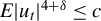 $ E|u_{t}|^{4+\delta }\le c$
for some
$ E|u_{t}|^{4+\delta }\le c$
for some $\delta>0$
, where
$\delta>0$
, where $c>0$
does not depend on
$c>0$
does not depend on $k,t,n$
.
$k,t,n$
.
(ii) $g_{kt} \ge c>0$
and
$g_{kt} \ge c>0$
and $h_{t} \ge c>0$
, where c does not depend on
$h_{t} \ge c>0$
, where c does not depend on $k,t,n$
.
$k,t,n$
.
(iii) $\varepsilon _t, \eta _t$
satisfy Assumptions 2.1, 2.2, and 2.4(i).
$\varepsilon _t, \eta _t$
satisfy Assumptions 2.1, 2.2, and 2.4(i).
Estimation of Fixed Parameters: Suppose that $y_t= \beta ^\prime z_t+u_t$
follows the regression model (1) with a fixed parameter
$y_t= \beta ^\prime z_t+u_t$
follows the regression model (1) with a fixed parameter $\beta $
as in Section 2. Our primary interest is to estimate the parameter
$\beta $
as in Section 2. Our primary interest is to estimate the parameter $\beta $
using the subsample (36). In view of (1), we can write the partially observed regression model as
$\beta $
using the subsample (36). In view of (1), we can write the partially observed regression model as
 $$ \begin{align} \widetilde y_t&= \tau_ty_t=\tau_t (\beta^\prime z_t +u_t),\nonumber \\ \widetilde y_t&= \beta^\prime \widetilde z_t +\widetilde u_t, \quad \widetilde u_t=\tau_tu_t=\{\tau_th_t\} \varepsilon_t. \end{align} $$
In (39), the regressors $\widetilde z_t$
and the noise
$\widetilde z_t$
and the noise $\widetilde u_t$
can be represented as
$\widetilde u_t$
can be represented as
 $$ \begin{align} \widetilde z_{kt}&= \widetilde \mu_{kt}+\widetilde g_{kt}\eta_{kt}, \quad \widetilde \mu_{kt}=\tau_t \mu_{kt}, \quad \widetilde g_{kt}=\tau_t g_{kt},\\ \widetilde u_{t}&= \widetilde h_{t}\varepsilon_{t}, \quad \widetilde h_{t}=\tau_t h_{t}. \nonumber \end{align} $$
They belong to the regression space described in (2) and (3). Therefore, parameter $\beta $
and the correspondent standard errors in model (39) can be estimated using the OLS estimator
$\beta $
and the correspondent standard errors in model (39) can be estimated using the OLS estimator $\widehat \beta $
and
$\widehat \beta $
and $\widehat \omega _{kk}$
:
$\widehat \omega _{kk}$
:
 $$ \begin{align} \widehat \beta&=\left( \sum_{t=1}^n \widetilde z_{t} \widetilde z_{t}^\prime\right)^{-1}\left( \sum_{t=1}^n \widetilde z_{t}\widetilde y_{t}\right),\quad \widehat \Omega_n= S_{\widetilde z\widetilde z}^{-1} S_{\widetilde z\widetilde z\widehat u \widehat u} S_{\widetilde z\widetilde z}^{-1}=(\widehat \omega_{jk}), \\ S_{\widetilde z\widetilde z}&=\sum_{t=1}^n\widetilde z_{t}\widetilde z^\prime_{t}, \quad S_{\widetilde z\widetilde z\widehat u \widehat u}= \sum_{t=1}^n \widetilde z_{t}\widetilde z^\prime_{t} \widehat u_{t}^2, \quad \widehat u_{t}=\widetilde y_{t}-\widehat \beta^\prime \widetilde z_{t}. \nonumber \end{align} $$
Theorem 4.1. The OLS estimator $\widehat \beta $
of the parameter
$\widehat \beta $
of the parameter $\beta $
in the regression model (39) with missing data has the following asymptotic properties. If Assumptions 4.1 and 4.2 hold and
$\beta $
in the regression model (39) with missing data has the following asymptotic properties. If Assumptions 4.1 and 4.2 hold and $n/N=O_p(1)$
, then, for
$n/N=O_p(1)$
, then, for $k=1, \ldots , p$
, as
$k=1, \ldots , p$
, as $n \rightarrow \infty $
,
$n \rightarrow \infty $
,
 $$ \begin{align} \frac{\widehat \beta_k -\beta_k}{\sqrt{\widehat \omega_{kk}}}\rightarrow _d \mathcal{N}(0, 1), \qquad \quad \sqrt{ \widehat \omega_{kk}}\asymp_p n^{-1/2}. \end{align} $$
Remark 4.1. Theorem 4.1 shows that ignoring missing data does not affect the estimation of the fixed parameter. That is, the researcher can compute the estimators $\widehat \beta $
and
$\widehat \beta $
and $\sqrt {\widehat \omega _{kk}}$
directly using subsample
$\sqrt {\widehat \omega _{kk}}$
directly using subsample $y_{k_j}, z_{k_j}, \, j=1, \ldots , N$
:
$y_{k_j}, z_{k_j}, \, j=1, \ldots , N$
:
 $$ \begin{align*} \widehat \beta&=\left( \sum_{j=1}^N z_{k_j} z_{k_j}^\prime\right)^{-1}\left( \sum_{j=1}^N z_{k_j} y_{k_j}\right),\quad \widehat \Omega_n= S_{*,zz}^{-1} S_{*,zz\widehat u \widehat u} S_{*,zz}^{-1}=(\widehat \omega_{jk}), \\ S_{*,zz}&=\sum_{j=1}^Nz_{k_j}z^\prime_{k_j}, \quad S_{*,zz\widehat u \widehat u}= \sum_{j=1}^N z_{k_j}z^\prime_{k_j} \widehat u_{k_j}^2, \quad \widehat u_{k_j}=y_{k_j}-\widehat \beta^\prime z_{k_j}. \nonumber \end{align*} $$
Estimation of Time-Varying Parameters: Assume now that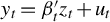 $y_t= \beta ^\prime _tz_t+u_t $
follows the regression model (21) with time-varying parameter
$y_t= \beta ^\prime _tz_t+u_t $
follows the regression model (21) with time-varying parameter $\beta _t$
, where regressors
$\beta _t$
, where regressors $z_t$
and regression noise
$z_t$
and regression noise $u_t$
are as in (3) and (2). We are interested in estimating the parameter
$u_t$
are as in (3) and (2). We are interested in estimating the parameter $\beta _t$
in the presence of missing data using the subsample (36). Similarly to (39), we base the estimation on the partially observed regression model with a time-varying parameter:
$\beta _t$
in the presence of missing data using the subsample (36). Similarly to (39), we base the estimation on the partially observed regression model with a time-varying parameter:
 $$ \begin{align} \widetilde y_j= \beta^\prime_j \widetilde z_j +\widetilde u_j, \quad j=1, \ldots, n, \end{align} $$
where regressors $\widetilde z_j$
and the noise
$\widetilde z_j$
and the noise $\widetilde u_j$
are defined as in (40). They belong to the regression space described by (2) and (3) and thus results of Section 3 on the estimation of the time-varying parameter
$\widetilde u_j$
are defined as in (40). They belong to the regression space described by (2) and (3) and thus results of Section 3 on the estimation of the time-varying parameter $\beta _j$
apply.
$\beta _j$
apply.
We show in the following theorem that under Assumptions 4.1 and 4.2, parameter $\beta _t$
and standard errors can be estimated point-wise at each time
$\beta _t$
and standard errors can be estimated point-wise at each time $t=1, \ldots , n$
provided that the missing data pattern satisfies the following condition:
$t=1, \ldots , n$
provided that the missing data pattern satisfies the following condition:
 $$ \begin{align} H/N_t=O_p(1), \quad\text{where} \,\,\, N_t=\sum_{j=1}^n \tau_j b_{n,tj}. \end{align} $$
This condition holds, for example, if $\tau _j=1$
for
$\tau _j=1$
for $|j-t|\le \epsilon H$
for some
$|j-t|\le \epsilon H$
for some $\epsilon>0$
.
$\epsilon>0$
.
The estimator $\widehat \beta _t$
and the estimator of the robust standard errors
$\widehat \beta _t$
and the estimator of the robust standard errors $\widehat \omega _{kk,t}$
given in (22) and (33) are defined as
$\widehat \omega _{kk,t}$
given in (22) and (33) are defined as
 $$ \begin{align} \widehat \beta_t&=\left( \sum_{j=1}^nb_{n,tj} \widetilde z_j \widetilde z_j^\prime\right)^{-1}\left( \sum_{j=1}^nb_{n,tj} \widetilde z_j \widetilde y_j\right),\\ \widehat \Omega_{nt}&=S_{\widetilde z\widetilde z,t}^{-1}S_{\widetilde z\widetilde z\widehat u \widehat u,t}S_{\widetilde z\widetilde z,t}^{-1}=(\widehat \omega_{jk,t}), \quad \widehat u_j=\widetilde y_j-\widehat \beta_j ^\prime \widetilde z_j. \nonumber \end{align} $$
Theorem 4.2. The OLS estimator $\widehat \beta _t $
of the time-varying parameter
$\widehat \beta _t $
of the time-varying parameter $\beta _t$
in the regression model (43) with missing data has the following properties. Assume that
$\beta _t$
in the regression model (43) with missing data has the following properties. Assume that $1\le t=t_n\le n$
, Assumptions 4.1, 3.1, and 4.2 are satisfied and that the condition
$1\le t=t_n\le n$
, Assumptions 4.1, 3.1, and 4.2 are satisfied and that the condition $H/N_t=O_p(1)$
holds. Then, for
$H/N_t=O_p(1)$
holds. Then, for $k=1, \ldots , p$
, as
$k=1, \ldots , p$
, as $n \rightarrow \infty $
,
$n \rightarrow \infty $
,
 $$ \begin{align} &\widehat \beta_{kt} -\beta_{kt}=O_p\big( H^{-1/2}+ (H/n)^\gamma\big), \end{align} $$
 $$ \begin{align} &\frac{\widehat \beta_{kt} -\beta_{kt}}{\sqrt{\widehat \omega_{kk,t}}}\rightarrow _d \mathcal{N}(0, 1)\quad \text{ if } H=o(n^{2\gamma/(2\gamma+1)}), \end{align} $$
 $$ \begin{align} &\widehat \omega_{kk,t}\asymp_p H^{-1}. \end{align} $$
5 ESTIMATION OF A STATIONARY AR(p) MODEL WITH AN m.d. NOISE
In this section, we focus on another practical application of our regression framework developed in Section 2. We show that it covers the estimation of the parameters of a stationary AR(p) model driven by a stationary m.d. noise $\varepsilon _t$
:
$\varepsilon _t$
:
 $$ \begin{align} y_t=\phi_0+\phi_1y_{t-1}+\cdots+\phi_py_{t-p}+\varepsilon_t, \end{align} $$
where parameters $\phi _0, \ldots , \phi _p$
are such that the model (49) has a stationary solution. Xu and Phillips (Reference Xu and Phillips2008) developed estimation theory for the AR
$\phi _0, \ldots , \phi _p$
are such that the model (49) has a stationary solution. Xu and Phillips (Reference Xu and Phillips2008) developed estimation theory for the AR $(p)$
model
$(p)$
model $y_t=\phi _0+\phi _1y_{t-1}+\cdots +\phi _py_{t-p}+u_t$
, when
$y_t=\phi _0+\phi _1y_{t-1}+\cdots +\phi _py_{t-p}+u_t$
, when $u_t=h_t\varepsilon _t$
and
$u_t=h_t\varepsilon _t$
and $h_t$
is a smoothly varying deterministic sequence, and the m.d. sequence
$h_t$
is a smoothly varying deterministic sequence, and the m.d. sequence $\varepsilon _t$
satisfies
$\varepsilon _t$
satisfies $E[\varepsilon _t^2|{\cal F}_{t-1}]=1$
a.s. Giraitis, Taniguchi, and Taqqu (Reference Giraitis, Kapetanios and Yates2018) were among the first to analyze the distortions of standard errors caused by m.d. noise in the estimation of ARMA models. This article shows that the variance of the parameter vector
$E[\varepsilon _t^2|{\cal F}_{t-1}]=1$
a.s. Giraitis, Taniguchi, and Taqqu (Reference Giraitis, Kapetanios and Yates2018) were among the first to analyze the distortions of standard errors caused by m.d. noise in the estimation of ARMA models. This article shows that the variance of the parameter vector $\phi $
converges to a well-defined limit; however, its complex structure complicates the estimation of the limiting variance and the corresponding standard errors in empirical applications. They restricted the estimation of standard errors to AR(1) and MA(1) models. In the case of an AR
$\phi $
converges to a well-defined limit; however, its complex structure complicates the estimation of the limiting variance and the corresponding standard errors in empirical applications. They restricted the estimation of standard errors to AR(1) and MA(1) models. In the case of an AR $(p)$
model, using our method, we are able to estimate standard errors for any p without relying on asymptotic approximations which is the main novelty and contribution of this section. Notice that the model (49) can be written as a special case of the regression model (1):
$(p)$
model, using our method, we are able to estimate standard errors for any p without relying on asymptotic approximations which is the main novelty and contribution of this section. Notice that the model (49) can be written as a special case of the regression model (1):
 $$ \begin{align} y_t=\beta^\prime z_t+u_t, \quad u_t=\varepsilon_t.\end{align} $$
Here, the parameter $\beta =(\beta _1, \ldots , \beta _{p+1})^\prime =(\phi _0, \ldots , \phi _p)^\prime $
is fixed, and the regressors
$\beta =(\beta _1, \ldots , \beta _{p+1})^\prime =(\phi _0, \ldots , \phi _p)^\prime $
is fixed, and the regressors $z_t=(z_{1t},z_{2t},\ldots ,z_{p+1,t})^ \prime =(1,y_{t-1},y_{t-2}, \ldots , y_{t-p})^\prime $
are stationary random variables. It is straightforward to verify that the regressors
$z_t=(z_{1t},z_{2t},\ldots ,z_{p+1,t})^ \prime =(1,y_{t-1},y_{t-2}, \ldots , y_{t-p})^\prime $
are stationary random variables. It is straightforward to verify that the regressors
 $$ \begin{align*}z_{kt}= \mu_{kt}+g_{kt}\eta_{kt}, \quad \mu_{kt}=E[y_{t-k}]=Ey_1, \quad g_{kt}=1, \quad \eta_{kt}=y_{t-k}-E[y_{t-k}] \end{align*} $$
for $k=2, \ldots , p+1$
satisfy the regression assumption (3). In the theorem below, we assume that the standard stationarity conditions on parameters of the AR(p) model (49) are satisfied, see for example, Theorem 3.1.1 in Brockwell and Davis (Reference Brockwell and Davis1991), which ensure the existence of a stationary solution
$k=2, \ldots , p+1$
satisfy the regression assumption (3). In the theorem below, we assume that the standard stationarity conditions on parameters of the AR(p) model (49) are satisfied, see for example, Theorem 3.1.1 in Brockwell and Davis (Reference Brockwell and Davis1991), which ensure the existence of a stationary solution
 $$ \begin{align} y_t=\mu+\sum_{j=0}^\infty a_j\varepsilon_{t-j}, \quad \text{where} \,\,\sum_{j=0}^\infty |a_j|<\infty, \,\,\mu=Ey_t. \end{align} $$
We assume that $\varepsilon _t$
satisfies Assumption 2.1 and
$\varepsilon _t$
satisfies Assumption 2.1 and $\eta _t=(y_{t-1},y_{t-2}, \ldots , y_{t-p})^\prime $
satisfies Assumptions 2.2 and 2.4(i). These assumptions impose only mild restrictions on the m.d. noise
$\eta _t=(y_{t-1},y_{t-2}, \ldots , y_{t-p})^\prime $
satisfies Assumptions 2.2 and 2.4(i). These assumptions impose only mild restrictions on the m.d. noise $\varepsilon _t$
, and their validity can be verified for typical examples of uncorrelated m.d. noise, such as ARCH-type processes.
$\varepsilon _t$
, and their validity can be verified for typical examples of uncorrelated m.d. noise, such as ARCH-type processes.
The OLS estimator $\widehat \beta $
of
$\widehat \beta $
of $\beta $
in the regression model (50) is defined as in (8) and
$\beta $
in the regression model (50) is defined as in (8) and $ \widehat \omega _{kk}$
as in (15).
$ \widehat \omega _{kk}$
as in (15).
Theorem 5.1. Suppose that the AR( p) model (49) with m.d. noise $\varepsilon _t$
has a stationary solution as in (51), that
$\varepsilon _t$
has a stationary solution as in (51), that $E\varepsilon _t^8<\infty $
and that
$E\varepsilon _t^8<\infty $
and that $(\varepsilon _t, \eta _t)$
satisfy Assumptions 2.1, 2.2, and 2.4(i). Then the OLS estimator
$(\varepsilon _t, \eta _t)$
satisfy Assumptions 2.1, 2.2, and 2.4(i). Then the OLS estimator $\widehat \beta $
of parameter
$\widehat \beta $
of parameter $\beta $
in regression model (50) has the following properties: for
$\beta $
in regression model (50) has the following properties: for $k=1, \ldots , p+1$
, as
$k=1, \ldots , p+1$
, as $n \rightarrow \infty $
,
$n \rightarrow \infty $
,
 $$ \begin{align} \frac{\widehat \beta_k -\beta_k}{\sqrt{\widehat \omega_{kk}}}\rightarrow _d \mathcal{N}(0, 1), \qquad \quad \sqrt{ \widehat \omega_{kk}}\asymp_p n^{-1/2}. \end{align} $$
The Monte Carlo results presented in Section 6.4 demonstrate that the robust OLS (ROLS) estimation produces correct $95\%$
confidence intervals for
$95\%$
confidence intervals for $\beta _k$
, whereas the standard OLS method exhibits coverage distortions when the noise
$\beta _k$
, whereas the standard OLS method exhibits coverage distortions when the noise $ \varepsilon _t$
is not i.i.d. This finding indicates that the ROLS estimator has a broader range of applicability than merely addressing heteroskedasticity, and that it can also be effectively used in regression settings not covered by the standard OLS estimation and inference theory.
$ \varepsilon _t$
is not i.i.d. This finding indicates that the ROLS estimator has a broader range of applicability than merely addressing heteroskedasticity, and that it can also be effectively used in regression settings not covered by the standard OLS estimation and inference theory.
It is worth noting that the papers by Doukhan and Wintenberger (Reference Doukhan and Wintenberger2008), Bardet and Wintenberger (Reference Bardet and Wintenberger2009), and Karmakar et al. (Reference Karmakar, Richter and Wu2022) provide advanced theoretical results on the modeling and estimation of general nonlinear time-varying time-series models; however, they address the linear AR $(p)$
model (49) only in the trivial case of an i.i.d. noise
$(p)$
model (49) only in the trivial case of an i.i.d. noise $\varepsilon _t$
.
$\varepsilon _t$
.
6 MONTE CARLO SIMULATIONS
In this section, we explore the finite-sample performance of the robust and standard OLS estimation methods in the regression settings, outlined in Sections 2 and 3. We examine the impact of time-varying deterministic and stochastic parameters, means, scale factors, and heteroskedasticity of the regression noise on estimation. A comparison of simulation results for standard and robust estimation methods shows that, despite the generality of our regression setting, estimation based on the robust standard errors produces well-sized confidence intervals for fixed and time-varying regression parameters $\beta $
and
$\beta $
and $\beta _{t}$
, while application of the standard confidence intervals leads to severe distortion of coverage rates.
$\beta _{t}$
, while application of the standard confidence intervals leads to severe distortion of coverage rates.
6.1 Estimation of a Fixed Parameter
We generate arrays of samples of regression models with fixed parameters and an intercept:
 $$ \begin{align} y_t=\beta_1+\beta_{2}z_{2t}+\beta_{3}z_{3t}+u_t, \quad u_t=h_t \varepsilon_t, \quad \beta=(\beta_1,\beta_2,\beta_3)^\prime= (0.5, 0.4 , 0.3)^\prime. \end{align} $$
We set the sample size to $n=1,500$
, conduct
$n=1,500$
, conduct $1,000$
replications, and set the nominal coverage probability at
$1,000$
replications, and set the nominal coverage probability at $0.95$
. (Estimation results for
$0.95$
. (Estimation results for $n=200, 800$
are available upon request.) We also include a more complex example in the Supplementary Material.
$n=200, 800$
are available upon request.) We also include a more complex example in the Supplementary Material.
This model includes three parameters and three regressors. We set $ z_{1t}=1$
and define
$ z_{1t}=1$
and define
 $$ \begin{align} z_{kt}&=\mu_{kt}+g_{kt}\eta_{kt},\,\,\,k=2,3, \\ \mu_{kt}&=0.5\sin(\pi t/n)+1, \quad \eta_{kt}= 0.5\eta_{k,t-1}+\xi_{kt}, \notag \end{align} $$
where $\xi _{2t}=\varepsilon _{t-1}$
and
$\xi _{2t}=\varepsilon _{t-1}$
and $\xi _{3t}=\varepsilon _{t-2}$
. The stationary m.d. noise
$\xi _{3t}=\varepsilon _{t-2}$
. The stationary m.d. noise $\varepsilon _t$
in
$\varepsilon _t$
in $u_t$
is generated by a GARCH(
$u_t$
is generated by a GARCH( $1,1$
) process
$1,1$
) process
 $$ \begin{align} \varepsilon_t =\sigma_t e_t, \quad \sigma^2_t = 1+0.7\sigma^2_{t-1}+0.2\varepsilon^2_{t-1}, \quad e_t\sim i.i.d.\,\mathcal{N} (0,1). \end{align} $$
Model 6.1. $y_t$
follows (53) with deterministic scale factors. We set
$y_t$
follows (53) with deterministic scale factors. We set $h_t=0.3(t/n)$
and
$h_t=0.3(t/n)$
and $g_{2t}=g_{3t}=0.4(t/n)$
.
$g_{2t}=g_{3t}=0.4(t/n)$
.
Model 6.2. $y_t$
follows (53) with stochastic scale factors. We set
$y_t$
follows (53) with stochastic scale factors. We set
 $$ \begin{align*} h_{t}=\Big|\dfrac{1}{2\sqrt{n}}\sum\limits^t_{j=1} \zeta_{j}\Big|+0.25, \quad g_{2t}=g_{3t}=\Big|\dfrac{1}{2\sqrt{n}}\sum\limits^t_{j=1} \nu_{kj} \Big|+0.25. \end{align*} $$
The generating noises $\{\zeta _{j},\, \nu _{2j}, \nu _{3j}\}$
are i.i.d.
$\{\zeta _{j},\, \nu _{2j}, \nu _{3j}\}$
are i.i.d. $\mathcal {N}(0,1)$
and independent of
$\mathcal {N}(0,1)$
and independent of $\{\varepsilon _{t}\}$
.
$\{\varepsilon _{t}\}$
.
Models 6.1 and 6.2 are regression models with fixed parameters. Examples of plots of the simulated dependent variable, regressors, and regression noise are shown in Figures 1 and 2 ( $z_{2t}$
and
$z_{2t}$
and $z_{3t}$
have similar patterns). To verify the validity of the asymptotic normal approximation of Corollary 2.1 in finite samples, we compute empirical coverage rates (CP) for
$z_{3t}$
have similar patterns). To verify the validity of the asymptotic normal approximation of Corollary 2.1 in finite samples, we compute empirical coverage rates (CP) for $95\%$
confidence intervals used in the ROLS estimation, for parameter
$95\%$
confidence intervals used in the ROLS estimation, for parameter $\beta $
. For comparison, we compute the coverage rates CP
$\beta $
. For comparison, we compute the coverage rates CP $_{st}$
for standard confidence intervals based on the standard errors (20) used in standard OLS estimation. The robust and standard OLS procedures share the same estimator
$_{st}$
for standard confidence intervals based on the standard errors (20) used in standard OLS estimation. The robust and standard OLS procedures share the same estimator $\widehat \beta $
, and hence the same bias, root mean square error (RMSE), and standard deviation (SD). Their confidence intervals differ because the variances (and standard errors) in their normal approximations are different.
$\widehat \beta $
, and hence the same bias, root mean square error (RMSE), and standard deviation (SD). Their confidence intervals differ because the variances (and standard errors) in their normal approximations are different.
Plots of $y_t$
,
$y_t$
, $z_{2t}$
, and
$z_{2t}$
, and $u_t$
in Model 6.1.
$u_t$
in Model 6.1.
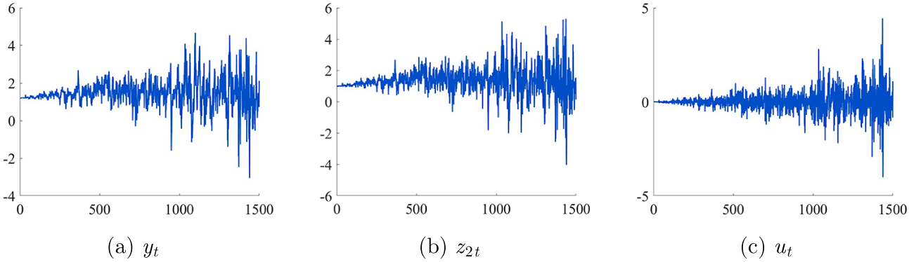
Plots of $y_t$
,
$y_t$
, $z_{2t}$
, and
$z_{2t}$
, and $u_t$
in Model 6.2.
$u_t$
in Model 6.2.
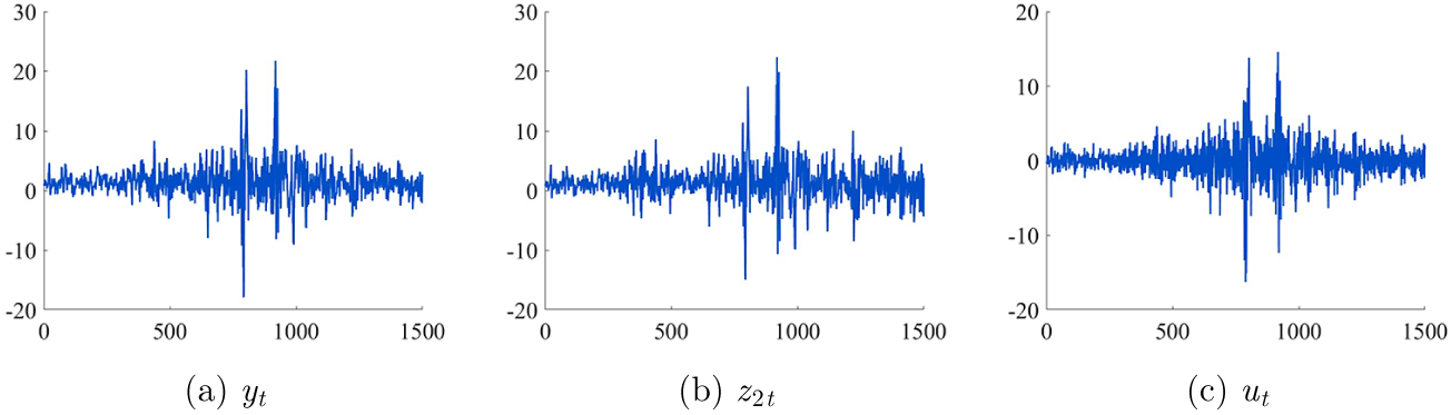
Table 1 reports estimation results for Model 6.1 which contains deterministic scale factors. It shows that the coverage rate CP for robust confidence intervals is close to the nominal $95\%$
, while the coverage rate CP
$95\%$
, while the coverage rate CP $_{st}$
of the standard confidence intervals drops below
$_{st}$
of the standard confidence intervals drops below $80\%$
. The Bias, RMSE, and SD are small.
$80\%$
. The Bias, RMSE, and SD are small.
Robust OLS estimation in Model 6.1

Table 2 presents estimation results for Model 6.2 which includes stochastic scale factors. It shows that the coverage rate CP for robust confidence intervals is close to the nominal $95\%$
, whereas the standard estimation method produces coverage distortions for parameters
$95\%$
, whereas the standard estimation method produces coverage distortions for parameters $\beta _2$
and
$\beta _2$
and $\beta _3$
.
$\beta _3$
.
Robust OLS estimation in Model 6.2

To assess power, we vary $\beta _3$
in Model 6.1 from
$\beta _3$
in Model 6.1 from $0$
to
$0$
to $0.5$
and record how often the test rejects
$0.5$
and record how often the test rejects $H_0: \beta _3=0$
. Figure 3 reports results for ROLS and OLS at sample sizes
$H_0: \beta _3=0$
. Figure 3 reports results for ROLS and OLS at sample sizes $n=200,\,800,\, 1,500$
. When
$n=200,\,800,\, 1,500$
. When $\beta _3=0$
, ROLS achieves a good size close to the nominal
$\beta _3=0$
, ROLS achieves a good size close to the nominal $5\%$
, while the size based on OLS results starts around
$5\%$
, while the size based on OLS results starts around $20\%$
and remains heavily oversized even as n increases. For
$20\%$
and remains heavily oversized even as n increases. For $\beta _3\neq 0$
, power rises monotonically with
$\beta _3\neq 0$
, power rises monotonically with $\beta _3$
for both methods. In Figure 3, the blue solid lines represent power based on ROLS, and the red solid lines correspond to standard OLS. Considering that the OLS estimation has large size distortion, we compute its adjusted power, shown by the red dotted lines. With a small sample size
$\beta _3$
for both methods. In Figure 3, the blue solid lines represent power based on ROLS, and the red solid lines correspond to standard OLS. Considering that the OLS estimation has large size distortion, we compute its adjusted power, shown by the red dotted lines. With a small sample size $n=200$
, OLS appears more powerful for
$n=200$
, OLS appears more powerful for $\beta _3 \le 0.2$
, whereas ROLS catches up and achieves good power when
$\beta _3 \le 0.2$
, whereas ROLS catches up and achieves good power when $\beta _3 \ge 0.3$
. For
$\beta _3 \ge 0.3$
. For $n=800$
and
$n=800$
and $1,500$
, both methods already achieve good power around
$1,500$
, both methods already achieve good power around $\beta _3=0.2$
. Overall, ROLS provides reliable size and competitive power across different sample sizes. Similar results are observed for Model 6.2.
$\beta _3=0.2$
. Overall, ROLS provides reliable size and competitive power across different sample sizes. Similar results are observed for Model 6.2.
Size, power, and adjusted power ( $\%$
) for the test
$\%$
) for the test $H_0: \beta _3=0$
in Model 6.1:
$H_0: \beta _3=0$
in Model 6.1: $\beta _3=0,\cdots ,0.5$
,
$\beta _3=0,\cdots ,0.5$
, $n=200,\,800,\, 1,500$
.
$n=200,\,800,\, 1,500$
.
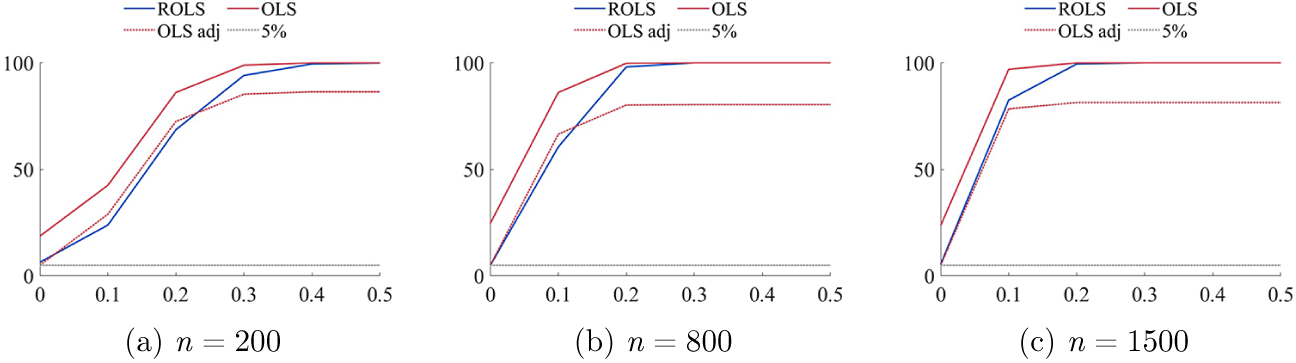
6.2 Estimation of a Time-Varying Parameter
In this section, we examine the validity of the normal approximation for the estimator $\widehat \beta _t$
, (22), of the time-varying parameter
$\widehat \beta _t$
, (22), of the time-varying parameter $\beta _t$
, as established in Corollary 3.1 of Section 3. We replace the fixed regression parameter
$\beta _t$
, as established in Corollary 3.1 of Section 3. We replace the fixed regression parameter $\beta $
in the model (53) by a time-varying parameter
$\beta $
in the model (53) by a time-varying parameter $ \beta _t=(\beta _{1t},\beta _{2t},\beta _{3t})^\prime $
:
$ \beta _t=(\beta _{1t},\beta _{2t},\beta _{3t})^\prime $
:
 $$ \begin{align} y_t=\beta_{1t}+\beta_{2t}z_{2t}+\beta_{3t}z_{3t}+u_t, \quad u_t=h_t \varepsilon_t, \end{align} $$
where $z_{1t}=1$
and
$z_{1t}=1$
and $z_{2t}, z_{3t}$
are defined using
$z_{2t}, z_{3t}$
are defined using $ \mu _{2t},\mu _{3t}$
and
$ \mu _{2t},\mu _{3t}$
and $\eta _{2t}, \eta _{3t}$
as in (54).
$\eta _{2t}, \eta _{3t}$
as in (54).
We consider two simulation models. Model 6.3 assumes deterministic parameters and scale factors, while Model 6.4 combines deterministic and stochastic parameters and scale factors.
Model 6.3. $y_t$
follows (56) with
$y_t$
follows (56) with $\varepsilon _t$
as in (55). The scale factors
$\varepsilon _t$
as in (55). The scale factors $h_t, g_{2t},g_{3t}$
and the parameters
$h_t, g_{2t},g_{3t}$
and the parameters $\beta _{1t}, \beta _{2t},\beta _{3t}$
are deterministic:
$\beta _{1t}, \beta _{2t},\beta _{3t}$
are deterministic:
 $$ \begin{align*} h_{t}&=0.5 \sin(2\pi t/n)+1, \quad g_{2t}=g_{3t}=0.5\sin(\pi t/n)+1. \\ \beta_{1t}&=0.5\sin(0.5\pi t/n)+1, \quad \beta_{2t}=0.5\sin(\pi t/n)+1,\quad \beta_{3t}= 0.5\sin(2\pi t/n)+1. \end{align*} $$
Model 6.4. $y_t$
follows (56) with
$y_t$
follows (56) with $\varepsilon _t \sim i.i.d. \,\mathcal {N} (0,1) $
and scale factors:
$\varepsilon _t \sim i.i.d. \,\mathcal {N} (0,1) $
and scale factors:
 $$ \begin{align*} h_{t}= 0.5 \sin(2\pi t/n)+1, \quad g_{2t}=\Big|n^{-\gamma}\sum\limits_{j=1}^{t}\zeta_{j}\Big|+0.2, \quad g_{3t}=0.5 \sin(\pi t/n)+1. \end{align*} $$
Parameters $\beta _{1t},\beta _{2t}$
are the same as in Model 6.3, while
$\beta _{1t},\beta _{2t}$
are the same as in Model 6.3, while $\beta _{3t}$
is stochastic:
$\beta _{3t}$
is stochastic:
 $$ \begin{align*} \beta_{3t}=\Big|n^{-\gamma}\sum\limits_{j=1}^{t}\nu_{j}\Big|+0.3(t/n), \end{align*} $$
where $\{\zeta _{j}\}, \{\nu _{j}\}$
are stationary ARFIMA
$\{\zeta _{j}\}, \{\nu _{j}\}$
are stationary ARFIMA $(0, d, 0)$
processes with memory parameter
$(0, d, 0)$
processes with memory parameter $d=0.4$
.
$d=0.4$
.
We estimate $\beta _t$
using the estimator
$\beta _t$
using the estimator $\widehat \beta _t$
, (22), where the weights
$\widehat \beta _t$
, (22), where the weights $b_{n,tj}= K(|t-j|/H) $
are computed with the Gaussian kernel function
$b_{n,tj}= K(|t-j|/H) $
are computed with the Gaussian kernel function $K(x)= (2\pi )^{-1/2}\exp (-x^2/2)$
with bandwidth
$K(x)= (2\pi )^{-1/2}\exp (-x^2/2)$
with bandwidth $ H=n^h$
,
$ H=n^h$
, $h=0.4, 0.5, 0.6, 0.7$
.
$h=0.4, 0.5, 0.6, 0.7$
.
Figure 4 displays parameter estimation results for a single simulation from Model 6.3. It depicts the estimates $\widehat \beta _{k1}, \ldots , \widehat \beta _{kn}$
(red line) against the true parameters
$\widehat \beta _{k1}, \ldots , \widehat \beta _{kn}$
(red line) against the true parameters $\beta _{kt}$
(blue line),
$\beta _{kt}$
(blue line), $k=1,2,3$
obtained with the bandwidth
$k=1,2,3$
obtained with the bandwidth $ H=n^{0.5}$
, and their point-wise
$ H=n^{0.5}$
, and their point-wise $95\%$
confidence intervals (gray dashed lines), computed using the robust standard errors. The robust time-varying confidence intervals cover the true parameters
$95\%$
confidence intervals (gray dashed lines), computed using the robust standard errors. The robust time-varying confidence intervals cover the true parameters $\beta _{kt}$
,
$\beta _{kt}$
, $t=1,\ldots ,n$
, for most of the time points.
$t=1,\ldots ,n$
, for most of the time points.
Robust 95 $\%$
confidence intervals for the time-varying parameters
$\%$
confidence intervals for the time-varying parameters $ \beta _{1t}, \beta _{2t}, \beta _{3t}$
in Model 6.3:
$ \beta _{1t}, \beta _{2t}, \beta _{3t}$
in Model 6.3: $n=1,500$
, bandwidth
$n=1,500$
, bandwidth $H=n^{0.5}$
. Single replication.
$H=n^{0.5}$
. Single replication.
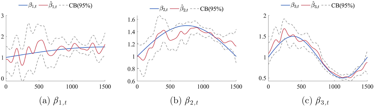
Figure 5 reports the point-wise empirical coverage rates (blue line) in the time-varying robust estimation of parameters $\beta _{kt},\, k=1,2,3$
, which are close to the nominal
$\beta _{kt},\, k=1,2,3$
, which are close to the nominal $95\%$
for most of the time points. Figure 6 shows the RMSEs for different choices of the bandwidth
$95\%$
for most of the time points. Figure 6 shows the RMSEs for different choices of the bandwidth $H=n^h$
,
$H=n^h$
, $h=0.4, 0.5, 0.6, 0.7$
. As expected, the RMSE depends on the smoothness of the parameter
$h=0.4, 0.5, 0.6, 0.7$
. As expected, the RMSE depends on the smoothness of the parameter $ \beta _{kt}$
and is often minimized by moderately large values of H, for example,
$ \beta _{kt}$
and is often minimized by moderately large values of H, for example, $H=n^{0.6}$
.
$H=n^{0.6}$
.
Coverage rates (in %) of robust confidence intervals for the time-varying parameters $ \beta _{1t}, \beta _{2t}, \beta _{3t}$
in Model 6.3:
$ \beta _{1t}, \beta _{2t}, \beta _{3t}$
in Model 6.3: $n=1,500$
, bandwidth
$n=1,500$
, bandwidth $H=n^{0.5}$
.
$H=n^{0.5}$
.
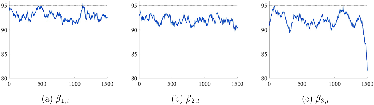
RMSE for the time-varying parameters $ \beta _{1t}, \beta _{2t}, \beta _{3t}$
in Model 6.3:
$ \beta _{1t}, \beta _{2t}, \beta _{3t}$
in Model 6.3: $n=1,500$
, bandwidth
$n=1,500$
, bandwidth $H=n^{h}$
,
$H=n^{h}$
, $h={0.4, 0.5, 0.6, 0.7}.$
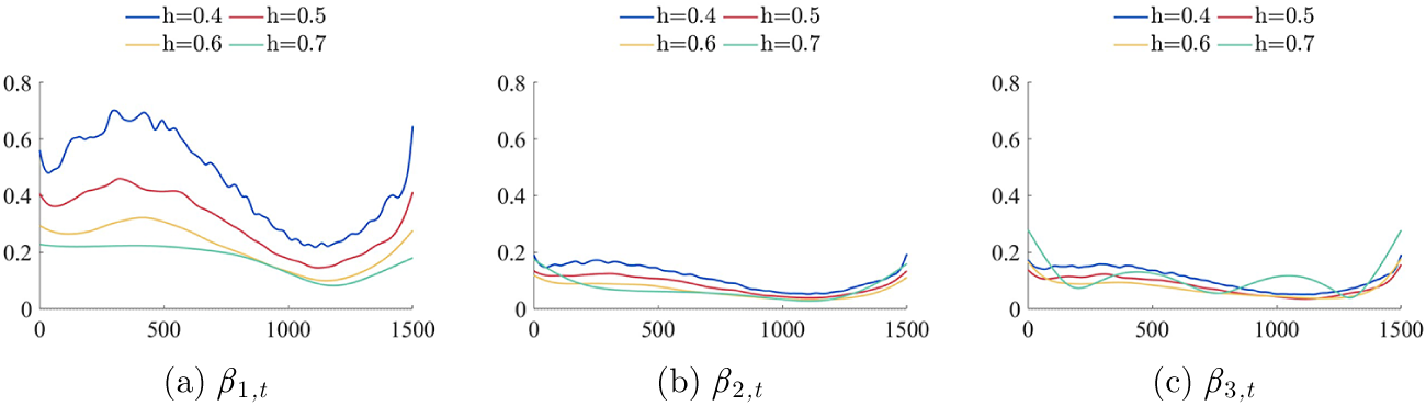
Figure 7 reports estimation results for a single simulation from Model 6.4, and Figure 8 displays point-wise empirical coverage rates for robust $95\% $
confidence intervals. For deterministic parameters
$95\% $
confidence intervals. For deterministic parameters $\beta _{1t}$
and
$\beta _{1t}$
and $\beta _{2t}$
, the estimation quality is good and the results are similar to those obtained for Model 6.3. For the stochastic parameter
$\beta _{2t}$
, the estimation quality is good and the results are similar to those obtained for Model 6.3. For the stochastic parameter $\beta _{3t}$
, the robust point-wise confidence intervals cover the path of stochastic parameter
$\beta _{3t}$
, the robust point-wise confidence intervals cover the path of stochastic parameter $\beta _{3t}$
for most of the time points (see Figure 7(c)). Figure 8(c) shows that coverage rates of robust time-varying confidence intervals for
$\beta _{3t}$
for most of the time points (see Figure 7(c)). Figure 8(c) shows that coverage rates of robust time-varying confidence intervals for $\beta _{3t}$
might be slightly affected by the stochastic variation in the parameter and scale factors. Nevertheless, they are still satisfactory and reasonably close to the nominal
$\beta _{3t}$
might be slightly affected by the stochastic variation in the parameter and scale factors. Nevertheless, they are still satisfactory and reasonably close to the nominal $95\%$
coverage.
$95\%$
coverage.
Robust 95 $\%$
confidence bands for the time-varying parameters
$\%$
confidence bands for the time-varying parameters $ \beta _{1t}, \beta _{2t}, \beta _{3t}$
in Model 6.4:
$ \beta _{1t}, \beta _{2t}, \beta _{3t}$
in Model 6.4: $n=1,500$
, bandwidth
$n=1,500$
, bandwidth $H=n^{0.5}$
. Single replication.
$H=n^{0.5}$
. Single replication.

Coverage rates (in %) of robust confidence intervals for the time-varying parameters $ \beta _{1t}, \beta _{2t}, \beta _{3t}$
in Model 6.4:
$ \beta _{1t}, \beta _{2t}, \beta _{3t}$
in Model 6.4: $n=1,500$
, bandwidth
$n=1,500$
, bandwidth $H=n^{0.5}$
.
$H=n^{0.5}$
.
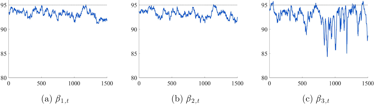
6.3 Estimation of Regression Parameters with Missing Data
To examine the impact of missing data on the robust and standard OLS estimation based on partially observed data $ (y_{j_1},z_{j_1}), (y_{j_2},z_{j_2}), \ldots , (y_{j_N},z_{j_N}), $
we use two types of missing data patterns over the time period
$ (y_{j_1},z_{j_1}), (y_{j_2},z_{j_2}), \ldots , (y_{j_N},z_{j_N}), $
we use two types of missing data patterns over the time period $1, \ldots , 1,500$
.
$1, \ldots , 1,500$
.
Type 1. The block of data $j\in [650, \,850]$
is missing.
$j\in [650, \,850]$
is missing.
Type 2. Five hundred single observations are missing at randomly selected times.
Tables 3 and 4 report robust and standard estimation results for Model 6.1 with a fixed parameter. Table 3 shows that block missing data (Type 1) do not lead to noticeable changes in bias, RMSE and SD, and the coverage rate for robust confidence intervals remains around $95\%$
. At the same time, the coverage rate CP
$95\%$
. At the same time, the coverage rate CP $_{st}$
of the standard confidence intervals is substantially distorted.
$_{st}$
of the standard confidence intervals is substantially distorted.
Robust OLS estimation in Model 6.1 with block missing data (Type 1)

Robust OLS estimation in Model 6.1 with randomly missing data (Type 2)

Table 4 shows that randomly missing data do not affect the coverage rate of robust confidence intervals which remains close to the nominal $95\%$
, while the coverage rate of the standard confidence intervals drops to around
$95\%$
, while the coverage rate of the standard confidence intervals drops to around $65\%$
. This emphasizes the flexibility of the ROLS estimation of the fixed parameter in the presence of block or randomly missing data.
$65\%$
. This emphasizes the flexibility of the ROLS estimation of the fixed parameter in the presence of block or randomly missing data.
Figures 9–11 report the estimation results for Model 6.3 with the time-varying parameter $\beta _t$
.
$\beta _t$
.
Coverage rates (in $\%$
) of robust confidence intervals for the time-varying parameters
$\%$
) of robust confidence intervals for the time-varying parameters $ \beta _{1t}, \beta _{2t}, \beta _{3t}$
in Model 6.3 with block missing data (Type 1),
$ \beta _{1t}, \beta _{2t}, \beta _{3t}$
in Model 6.3 with block missing data (Type 1), $n=1,500$
, bandwidth
$n=1,500$
, bandwidth $H=n^{0.5}$
.
$H=n^{0.5}$
.
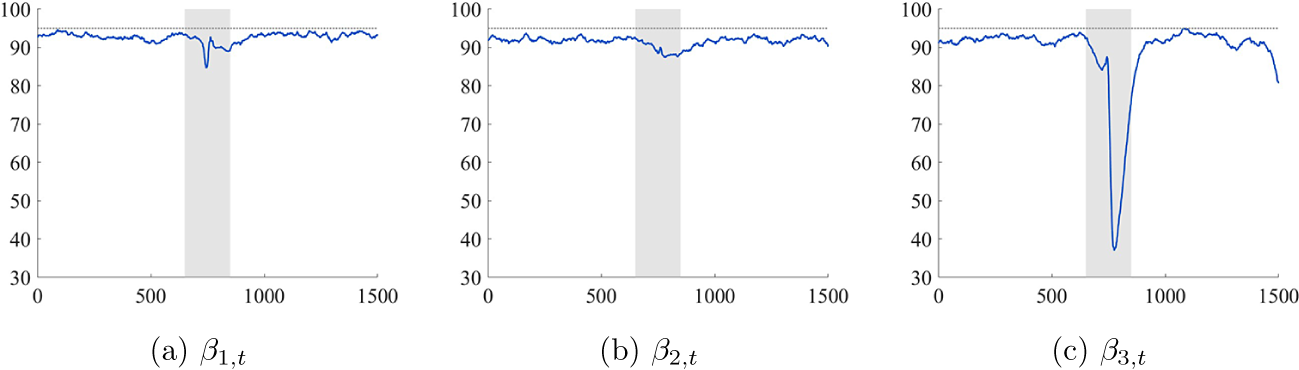
Robust 95 $\%$
confidence bands for the time-varying parameters
$\%$
confidence bands for the time-varying parameters $ \beta _{1t}, \beta _{2t}, \beta _{3t}$
in Model 6.3 with block missing data (Type 1),
$ \beta _{1t}, \beta _{2t}, \beta _{3t}$
in Model 6.3 with block missing data (Type 1), $n=1,500$
, bandwidth
$n=1,500$
, bandwidth $H=n^{0.5}$
. Single replication.
$H=n^{0.5}$
. Single replication.
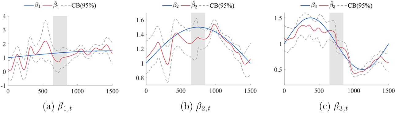
Figure 9 shows the coverage rates in time-varying robust estimation with block missing data (Type 1, shaded region) for $t=1, \ldots , 1,500$
. The coverage is close to the nominal
$t=1, \ldots , 1,500$
. The coverage is close to the nominal $95\%$
, with some distortion for parameters
$95\%$
, with some distortion for parameters $\beta _{1,t}$
and
$\beta _{1,t}$
and $\beta _{2,t}$
and a larger distortion for
$\beta _{2,t}$
and a larger distortion for $\beta _{3,t}$
within the shaded region. The distortion peaks at the center of the block, as expected. Although the width of the missing data block,
$\beta _{3,t}$
within the shaded region. The distortion peaks at the center of the block, as expected. Although the width of the missing data block, $200$
, exceeds the bandwidth
$200$
, exceeds the bandwidth $H=n^{0.5}=39$
used in estimating
$H=n^{0.5}=39$
used in estimating $\beta _t$
, the coverage distortion seems to be offset by the smooth down-weighting of the data, and the performance of the robust time-varying OLS estimation exceeds expectations.
$\beta _t$
, the coverage distortion seems to be offset by the smooth down-weighting of the data, and the performance of the robust time-varying OLS estimation exceeds expectations.
Coverage rates (in $\%$
) of robust confidence intervals for the time-varying parameters
$\%$
) of robust confidence intervals for the time-varying parameters $ \beta _{1t}, \beta _{2t}, \beta _{3t}$
in Model 6.3,
$ \beta _{1t}, \beta _{2t}, \beta _{3t}$
in Model 6.3, $500$
randomly missing data,
$500$
randomly missing data, $n=1,500$
, bandwidth
$n=1,500$
, bandwidth $H=n^{0.5}$
.
$H=n^{0.5}$
.
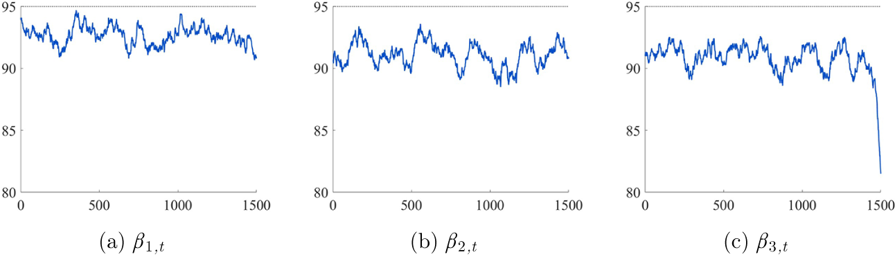
Figure 10 reports the path of the estimator $\widehat \beta _{kt}$
and the point-wise robust confidence intervals, for a single simulation. The robust confidence intervals become wider in the shaded region, which likely explains the satisfactory coverage performance during that period.
$\widehat \beta _{kt}$
and the point-wise robust confidence intervals, for a single simulation. The robust confidence intervals become wider in the shaded region, which likely explains the satisfactory coverage performance during that period.
Figure 11 shows that randomly missing data (Type 2) do not distort the robust time-varying OLS estimation. For all three parameters and time periods t, the coverage rate is close to the nominal. Overall, the robust estimation of time-varying parameters does not appear to be affected by randomly missing data.
6.4 Estimation of a Stationary AR(p) Model
We assess the performance of the robust and standard procedures in the case of a stationary AR( $2$
) model:
$2$
) model:
 $$ \begin{align} y_t=\beta_1+\beta_{2}y_{t-1}+\beta_{3}y_{t-2}+\varepsilon_t, \quad \beta=(\beta_1,\beta_2, \beta_3)^\prime= (0.5, 0.4 , 0.3)^\prime, \end{align} $$
where $\varepsilon _t=e_te_{t-1}$
,
$\varepsilon _t=e_te_{t-1}$
, $e_t\sim i.i.d. \,\mathcal {N}(0,1)$
is a stationary m.d. noise. The regressors
$e_t\sim i.i.d. \,\mathcal {N}(0,1)$
is a stationary m.d. noise. The regressors $z_t=(z_{1,t},z_{2,t},z_{3,t})^\prime =(1,y_{t-1},y_{t-2})^ \prime $
include an intercept and the two past lags of
$z_t=(z_{1,t},z_{2,t},z_{3,t})^\prime =(1,y_{t-1},y_{t-2})^ \prime $
include an intercept and the two past lags of $y_t$
. By Theorem 5.1, the parameter
$y_t$
. By Theorem 5.1, the parameter $\beta $
can be estimated by using the robust estimation method.
$\beta $
can be estimated by using the robust estimation method.
Table 5 shows that the coverage rate for the ROLS estimation is close to the nominal $95\%$
, while the standard OLS estimation exhibits extensive coverage distortion for
$95\%$
, while the standard OLS estimation exhibits extensive coverage distortion for $\beta _2$
and
$\beta _2$
and $\beta _3$
.
$\beta _3$
.
Robust OLS estimation in the $AR(2)$
model (57)
$AR(2)$
model (57)

7 EMPIRICAL EXPERIMENT
In this section, we analyze the structure and dynamics of daily S $\&$
P 500 log returns,
$\&$
P 500 log returns, $r_t$
, from 2 January 1990 to 31 December 2019 (sample size
$r_t$
, from 2 January 1990 to 31 December 2019 (sample size $n=7,558$
). We employ robust regression estimation to assess whether the returns
$n=7,558$
). We employ robust regression estimation to assess whether the returns $r_t$
can be modeled using a time-varying regression model of the form
$r_t$
can be modeled using a time-varying regression model of the form
 $$ \begin{align} r_t=\mu_t+u_t,\quad u_t=h_t\varepsilon_t, \end{align} $$
where $\{\varepsilon _t\}$
is an i.i.d.
$\{\varepsilon _t\}$
is an i.i.d. $(0,1)$
noise, and the time-varying mean
$(0,1)$
noise, and the time-varying mean $\mu _t$
and scale factor
$\mu _t$
and scale factor $h_t$
are independent of
$h_t$
are independent of $\{\varepsilon _t\}$
. Our objective is to estimate the time-varying mean
$\{\varepsilon _t\}$
. Our objective is to estimate the time-varying mean $\mu _t$
, the scale factor
$\mu _t$
, the scale factor $h_t$
, and to test for the absence of autocorrelation in the centered absolute residuals
$h_t$
, and to test for the absence of autocorrelation in the centered absolute residuals $\widetilde u_t=h_t(|\varepsilon _t|-E|\varepsilon _t|)$
, thereby assessing the fit of the model (58) to the data.
$\widetilde u_t=h_t(|\varepsilon _t|-E|\varepsilon _t|)$
, thereby assessing the fit of the model (58) to the data.
If returns $r_t$
follow the model (58) with i.i.d. noise
$r_t$
follow the model (58) with i.i.d. noise $\varepsilon _t$
, then
$\varepsilon _t$
, then $\widetilde u_t$
are uncorrelated for
$\widetilde u_t$
are uncorrelated for $t\ne s$
:
$t\ne s$
:
 $$ \begin{align*} \mathrm{cov}(\widetilde u_t, \widetilde u_s) = E\big[h_th_s\mathrm{cov}(|\varepsilon_t|,|\varepsilon_s|)\big]=0. \end{align*} $$
Conversely, if the noise $\varepsilon _t$
exhibits ARCH effects (stationary conditional heteroskedasticity), the sequence
$\varepsilon _t$
exhibits ARCH effects (stationary conditional heteroskedasticity), the sequence $|\varepsilon _t|$
becomes autocorrelated, and the null hypothesis of uncorrelated centered absolute residuals
$|\varepsilon _t|$
becomes autocorrelated, and the null hypothesis of uncorrelated centered absolute residuals $\widetilde u_t$
would be rejected.
$\widetilde u_t$
would be rejected.
We estimate the time-varying mean $\mu _{t}$
using the time-varying OLS estimator with bandwidths
$\mu _{t}$
using the time-varying OLS estimator with bandwidths $H=n^{0.4}, n^{0.5}, \ldots , n^{0.7}$
. Figure 12(a) shows the estimated path of
$H=n^{0.4}, n^{0.5}, \ldots , n^{0.7}$
. Figure 12(a) shows the estimated path of $\widehat \mu _{t}$
and the associated
$\widehat \mu _{t}$
and the associated $95\%$
confidence intervals for bandwidth
$95\%$
confidence intervals for bandwidth $H=n^{0.6}$
indicating that
$H=n^{0.6}$
indicating that $\mu _{t}$
is very likely to change over time.
$\mu _{t}$
is very likely to change over time.





Assumptions on model (58) imply that
 $$ \begin{align*} |u_t|=|r_t- \mu_t| = h_t|\varepsilon_t|= h_tE|\varepsilon_t|+h_t(|\varepsilon_t|-E|\varepsilon_t|). \end{align*} $$
Therefore, $|\widehat u_t|=|r_t-\widehat \mu _t| \sim h_tE|\varepsilon _t|+h_t(|\varepsilon _t|-E|\varepsilon _t|)$
and thus
$|\widehat u_t|=|r_t-\widehat \mu _t| \sim h_tE|\varepsilon _t|+h_t(|\varepsilon _t|-E|\varepsilon _t|)$
and thus $ y_t=|\widehat u_t|$
follows a time-varying regression model of the form
$ y_t=|\widehat u_t|$
follows a time-varying regression model of the form
 $$ \begin{align} y_t=\beta_{1t}+\widetilde u_t, \quad \widetilde u_t=g_t\eta_t, \end{align} $$
where $\beta _{1t}=h_tE|\varepsilon _t|$
represents a time-varying intercept,
$\beta _{1t}=h_tE|\varepsilon _t|$
represents a time-varying intercept, $ g_{t}=h_t $
denotes the scale factor, and
$ g_{t}=h_t $
denotes the scale factor, and $\eta _t=|\varepsilon _t|-E|\varepsilon _t|$
is an i.i.d. noise. Hence,
$\eta _t=|\varepsilon _t|-E|\varepsilon _t|$
is an i.i.d. noise. Hence, $\beta _{1t}$
can be consistently estimated using the time-varying OLS estimator
$\beta _{1t}$
can be consistently estimated using the time-varying OLS estimator $ \widehat \beta _{1t}$
. Figure 12(b) displays the estimated path of
$ \widehat \beta _{1t}$
. Figure 12(b) displays the estimated path of $\widehat {\beta }_{1t}$
and the corresponding
$\widehat {\beta }_{1t}$
and the corresponding $95\%$
confidence intervals for
$95\%$
confidence intervals for $\beta _{1t}=h_tE|\varepsilon _t|$
with bandwidth
$\beta _{1t}=h_tE|\varepsilon _t|$
with bandwidth $H=n^{0.6}$
, revealing pronounced time variation in the scale factor
$H=n^{0.6}$
, revealing pronounced time variation in the scale factor $h_t$
.
$h_t$
.
Figure 13(a) reports test results for zero correlation at lags $k=1, \ldots ,20$
in the residual sequence
$k=1, \ldots ,20$
in the residual sequence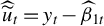 $\widehat {\widetilde {u}} _t=y_t-\widehat \beta _{1t}$
. We employ the standard and robust test procedures developed in Giraitis et al. (Reference Giraitis, Li and Phillips2024). Given that the sample size is large (
$\widehat {\widetilde {u}} _t=y_t-\widehat \beta _{1t}$
. We employ the standard and robust test procedures developed in Giraitis et al. (Reference Giraitis, Li and Phillips2024). Given that the sample size is large ( $n=7,558$
) and
$n=7,558$
) and $\beta _{1t}$
is estimated non-parametrically with bandwidth
$\beta _{1t}$
is estimated non-parametrically with bandwidth $H=n^{0.6}$
, we restrict the correlation analysis to the subsample
$H=n^{0.6}$
, we restrict the correlation analysis to the subsample $j\in [500,1000]$
. Both tests provide no evidence of significant correlation within this subsample, suggesting that the model (58) fits the returns
$j\in [500,1000]$
. Both tests provide no evidence of significant correlation within this subsample, suggesting that the model (58) fits the returns $r_t$
well during this time period.
$r_t$
well during this time period.
Robust and standard tests for the absence of correlation in the subsample of residuals $ \widehat { \widetilde {u}}_j$
,
$ \widehat { \widetilde {u}}_j$
, $ \widehat u^{*}_j$
,
$ \widehat u^{*}_j$
, $j\in [500,1000]$
,
$j\in [500,1000]$
, $H=n^{0.6}$
, significance level
$H=n^{0.6}$
, significance level $5\%$
.
$5\%$
.
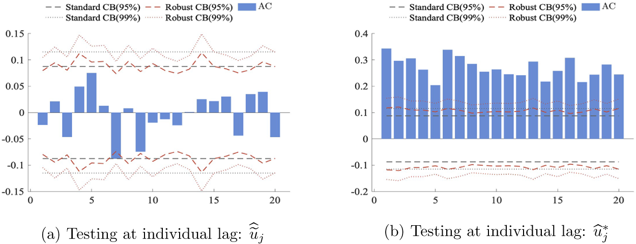
The same is not likely to be true if $r_t^*=r_t-\widehat \mu _t$
follows a GARCH(1,1) process, as confirmed by the following experiment. We fit a GARCH(1,1) model to the demeaned returns
$r_t^*=r_t-\widehat \mu _t$
follows a GARCH(1,1) process, as confirmed by the following experiment. We fit a GARCH(1,1) model to the demeaned returns $r_t^*=r_t-\widehat \mu _t$
:
$r_t^*=r_t-\widehat \mu _t$
:
 $$ \begin{align*} r^*_t=\sigma_t\varepsilon_t,\quad \sigma^2_t=1.563\times 10^{-6}+0.88913 \sigma^2_{t-1}+0.096974r^{*\,2}_{t-1}. \end{align*} $$
We generate a simulated GARCH(1,1) sample $r^*_{g 1}, \ldots , r^*_{g n}$
, apply the regression model (59) to the absolute values
$r^*_{g 1}, \ldots , r^*_{g n}$
, apply the regression model (59) to the absolute values $ y_t^*=|r^*_{g t}|$
, and compute the residuals,
$ y_t^*=|r^*_{g t}|$
, and compute the residuals, $\widehat {u} ^*_t=y_t^*-\widehat \beta _{1t}$
. Figure 13(b) shows that both standard and robust tests detect significant correlation in the residuals
$\widehat {u} ^*_t=y_t^*-\widehat \beta _{1t}$
. Figure 13(b) shows that both standard and robust tests detect significant correlation in the residuals $\widehat u^*_t$
, confirming the presence of conditional heteroskedasticity in the simulated GARCH data.
$\widehat u^*_t$
, confirming the presence of conditional heteroskedasticity in the simulated GARCH data.
8 CONCLUSION
The ROLS and time-varying OLS estimation and inference methods developed in this article offer considerable flexibility for modeling economic and financial data. They allow for general heterogeneity in regression components and for structural change in regression coefficients over time. Moreover, the generalization of the structure of regressors and error terms further expands the range of empirical settings to which the ROLS regression framework can be applied. In particular, the article develops asymptotic theory for general regression models with stochastic regressors, possibly including a time-varying mean, and provides data-based robust standard errors that enable the construction of confidence intervals for the regression parameters. The Monte Carlo analysis demonstrates the strong performance of the robust estimation approach under complex settings, and confirms the consistency and asymptotic normality property of the proposed estimators.
COMPETING INTEREST STATEMENT
The authors declare that no competing interests exist.
FUNDING STATEMENT
The authors declare that no specific funding has been received for this article.
SUPPLEMENTARY MATERIAL
Proofs of all results and some additional simulations are provided in Giraitis, L., Kapetanios, G., Li, Y., & Ventouri, A. (2025). Supplement to “Unlocking the Regression Space,” Econometric Theory Supplementary Material. To view, please visit: https://doi.org/10.1017/S0266466626100395.
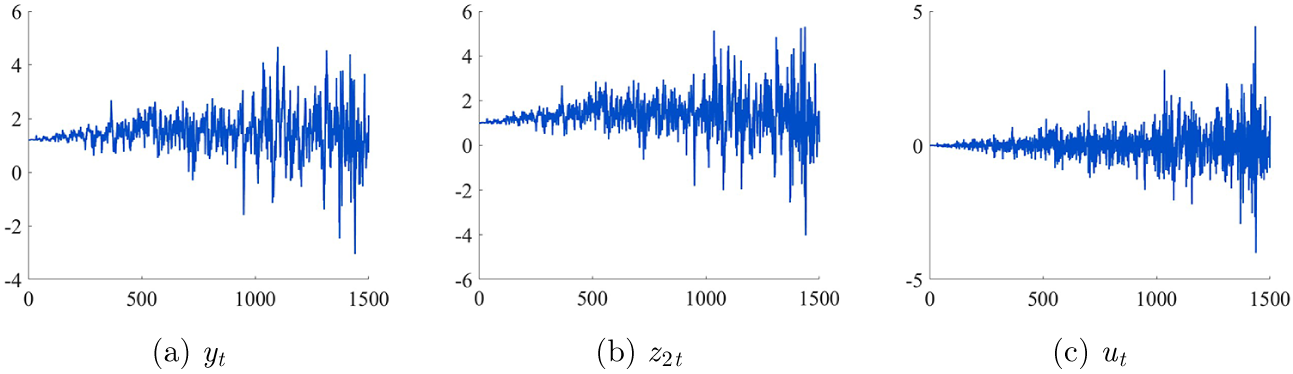


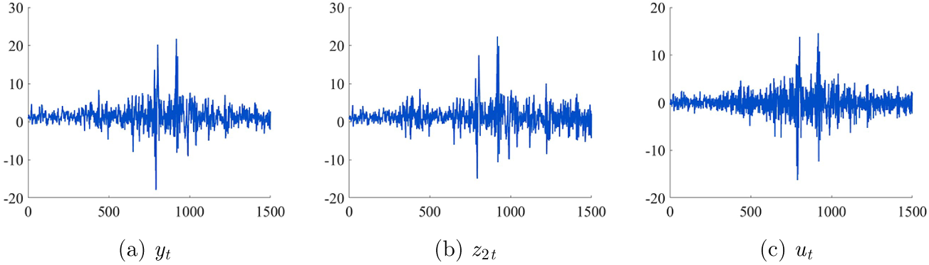




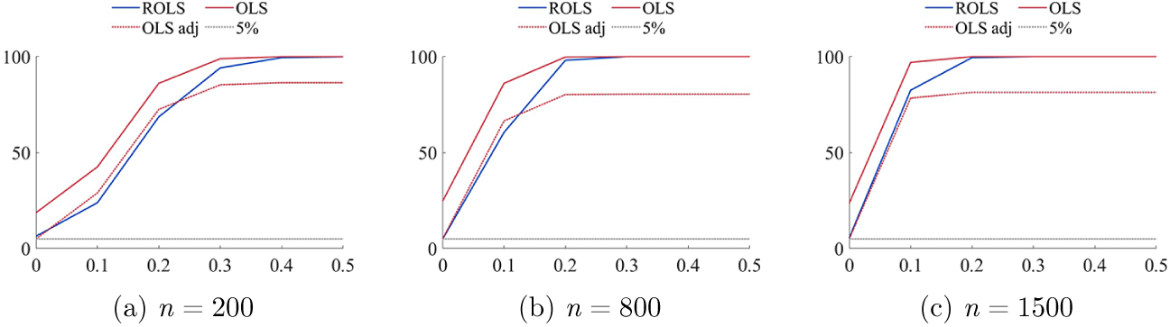


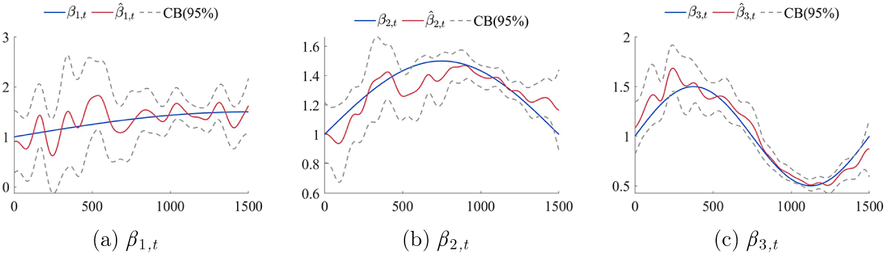


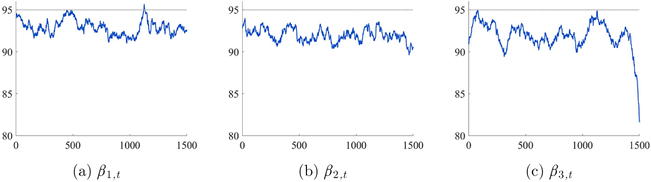


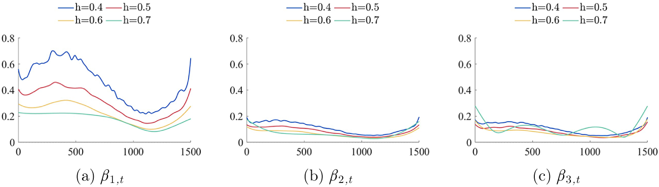


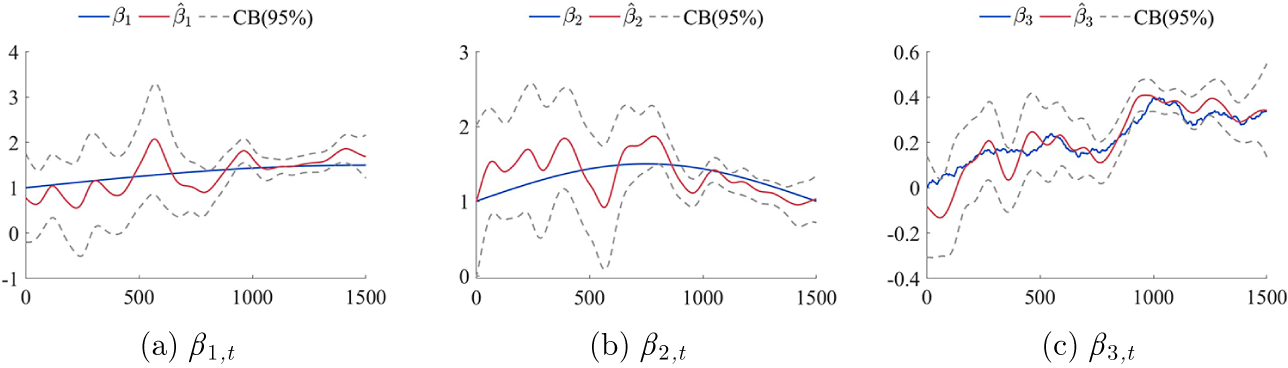


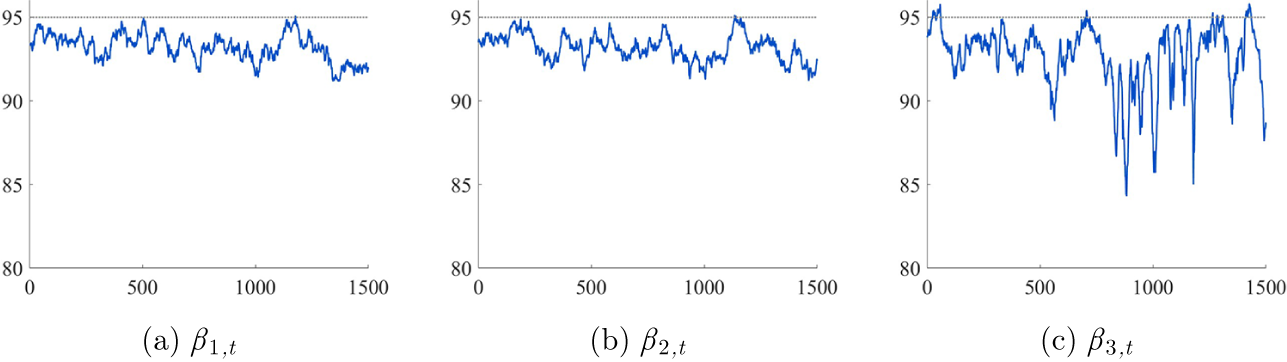




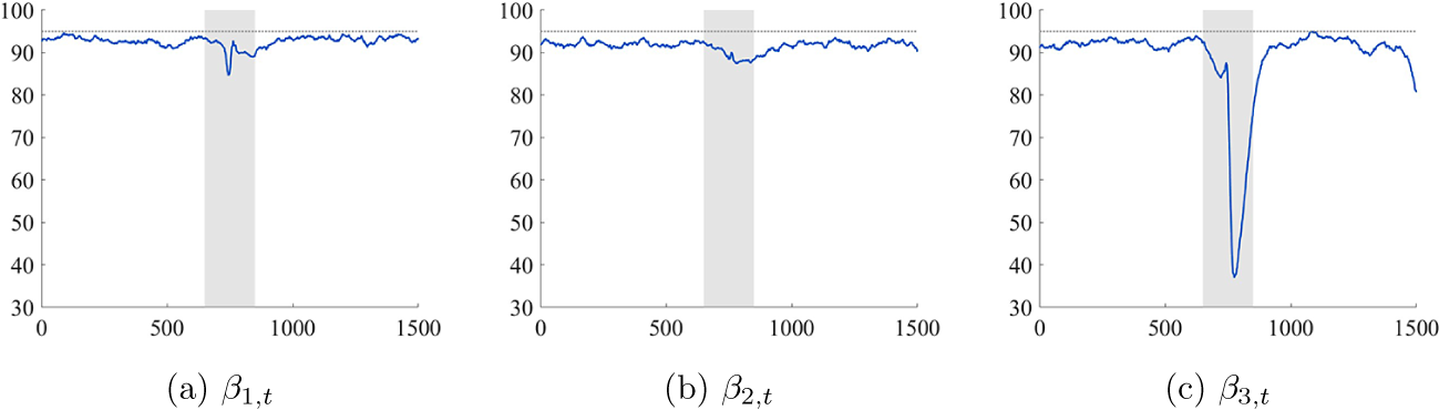


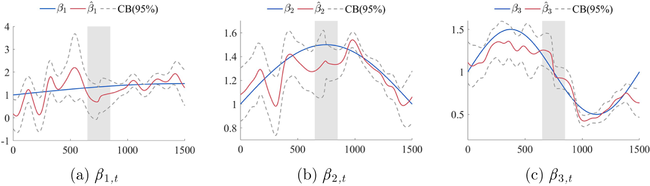


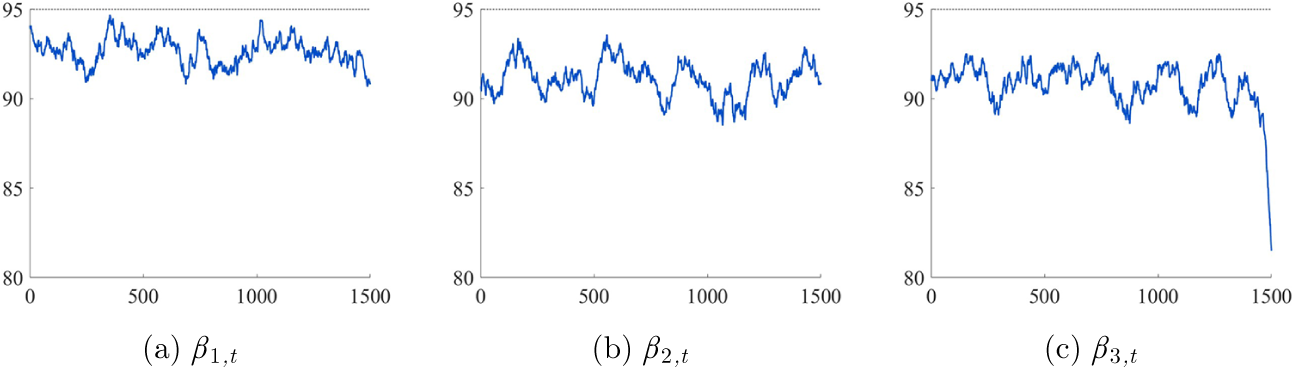




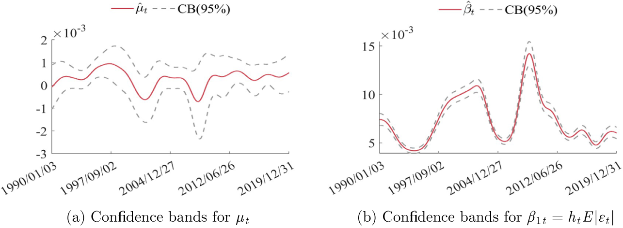


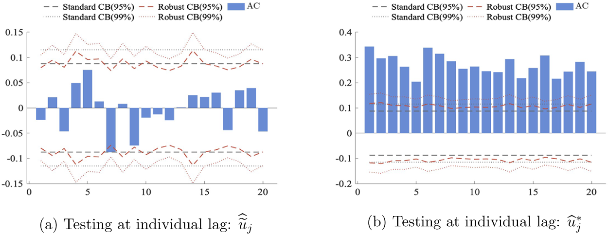


 Open access

