


In developed economies, the state plays a fundamental role by providing infrastructure, justice, healthcare, and education. To do this, the state needs financing. In the words of Besley and Persson (Reference Besley, Persson, Auerbach, Chetty, Feldstein and Saez2013, p. 51), ‘The central question in taxation and development is: how does a government go from raising around 10 percent of GDP in taxes to raising around 40 percent?’ To answer questions such as this, researchers need systematic information about how states financed themselves in the past and how state finance evolved over time. In many of today’s rich countries, fiscal modernization occurred in the 19th and early 20th centuries. Taxation is central to research on state-building – for example, how bargaining over taxation is related to limited government (Cox Reference Cox2016) – but is also crucial for understanding distributive conflict and democratization (eg Acemoglu and Robinson Reference Acemoglu and Robinson2001; Bates and Lien Reference Bates and Lien1985), and how war is related to fiscal fairness (Scheve and Stasavage Reference Scheve and Stasavage2016). In other words, politics is not only about who gets what, when and how (Lasswell Reference Lasswell1936) but also about who pays. Recently, there has been a renewed interest in the politics of taxation and in historical approaches to political science, as exemplified by the two recent handbooks by Hakelberg and Seelkopf (Reference Hakelberg and Seelkopf2021) and Jenkins and Rubin (Reference Jenkins and Rubin2024).
Despite the centrality of public finances in exploring a range of topics (eg Lee and Paine Reference Lee and Paine2023; Queralt Reference Queralt2022), existing datasets suffer from major drawbacks. Datasets containing high-quality, comparative information only cover recent periods (IMF, for instance, starts in 1972). Historical efforts go back further but cover only a small group of countries and include only total tax revenues and not their composition. For instance, Dincecco (Reference Dincecco2009) covers the period from 1650 to 1913 but provides information only on total central tax revenues and only for 11 European countries. Others rely on the information in Mitchell (Reference Mitchell2007a), information which is often unreliable. An important limitation for previous scholars seeking to explain the rise of the fiscal state in the 19th and 20th centuries is the lack of fine-grained tax data. For instance, Beramendi, Dincecco and Rogers (Reference Beramendi, Dincecco and Rogers2019) present a theory of elite competition and income taxation but can only evaluate it using data on all direct taxes (including income and land taxes) combined.
This research note presents a solution to these problems: the Govrev dataset. It provides information on tax revenues and their composition from 1800 to 2012. This period covers the emergence of modern parliamentary democracy and the welfare state. Beyond total revenues, it provides data on shares from income, property, customs, excises, and broad-based consumption taxes. It covers not only European countries but also all major states in the Americas as well as Australia, New Zealand, and Japan. This broad geographic and temporal scope allows analysts to track a global sample of countries from having a minimal state apparatus financed by tariffs to – in many cases – having large welfare states financed by modern taxes on income and consumption.
We make three main contributions.Footnote 1 First, we move beyond Western Europe by including 31 sovereign countries across the globe.Footnote 2 Second, in contrast to modern datasets, which usually cover many countries but only for a few decades, Govrev goes back to the early 19th century. Third, we provide detailed information on subcategories, allowing for a more comprehensive understanding of distributive politics and the rise of the modern tax state.
In the following sections, we present the dataset, how it was constructed and how it compares with previous efforts. We then use it to reevaluate the relationship between elite competition and direct taxation analyzed in Beramendi, Dincecco and Rogers (Reference Beramendi, Dincecco and Rogers2019) (henceforth, BDR). The final section concludes.
Measuring government budgets
We follow the World Bank (1988) and define taxes as ‘unrequited, compulsory payments collected primarily by central governments’. This clearly delineates taxation from fees in exchange for specific services and from natural resource rents. Moreover, we cover central government tax revenues only.Footnote 3 Total tax revenues are disaggregated into the following categories. First, we are interested in total tax revenue (nominally and as a share of GDP), as well as the shares of revenue coming from direct and indirect taxes. Second, we measure two subcategories of direct taxation: property and income. Third, for indirect taxes we separate excises (such as a salt tax), broad-based consumption taxes (eg value-added taxes (VATs)), and tariffs.Footnote 4
Collecting data for many countries over a long time span presents challenges regarding measurement and consistency. When different sources of data are combined, there need to be decisions about which sources to use and how to judge their quality. In addition, combining diverse sources may introduce measurement error and potentially bias the constructed estimates. Rather than averaging across sources when more than one source is available – which can increase rather than reduce measurement error – we followed a decision tree to decide which sources to use as the basis for our estimates. Keeping in mind our goal of connecting historical time series to contemporary high-quality datasets (such as from the OECD, the IMF, and CEPAL), we were guided by four rules: (1) minimize the number of sources, (2) prefer high-quality sources, (3) check the consistency of sources, and (4) time-series consistency trumps cross-sectional consistency.
The first rule is useful for two reasons. Since many sources rely on the same underlying data, averaging across sources might overstate the number of sources while potentially overweighting some sources with better temporal coverage. When two sources differ widely – for instance Mitchell and Johansen which is discussed later in this note – taking the average of the two is unlikely to be the best solution. Instead, we tried to understand why the sources differed and use the one which we deemed more trustworthy. Given that we decided against averaging, we also wanted to minimize the number of sources (while keeping over time coverage). One of the reasons for this is that sources differ in the level of detail they provide. Some only report large aggregates such as the share of direct tax revenue, without explaining what goes into that category. Sources may differ in aggregation rules, conceptualization of taxes, or in what underlying data is used. Minimizing the number of sources used increases the likelihood that a budget item is measured consistently over time. Constantly switching between sources may risk introducing measurement error based on small differences in aggregation rules or how taxes are classified.
What the second rule implies in practice is that we give primacy to primary and country-specific secondary information, especially if detailed sources and explanations are provided. These sources are often more fine-grained and more specific about the estimates they present. When we used existing cross-national datasets, we judged the quality of these by comparing their estimates to country-specific sources, high-quality contemporary data such as that provided by the OECD, and by scrutinizing their estimates. In cases when there was significant volatility in the reported estimates, we used country-specific information to ascertain whether a dramatic change in the series reflected a real change (eg war or fiscal reform) or some issue with the underlying data. In other instances, it was more straightforward that there was something in the construction of the database that was to blame, such as when revenue categories summed to more than 100 percent.
The fourth rule follows from our interest in understanding long-run trends within countries. In the occasional case of deciding between using the same source to reach cross-country consistency and employing different sources to obtain consistent within-country estimates, we prefer to emphasize time series consistency. This is also reflected in our preference for high-quality country-specific sources. Thus, we tried as far as possible to make sure that long-run trends within countries are not caused by changes in sources over time.
The goal of the data collection is to join historical data series to high-quality current databases to allow easy updating of the database in the future. In all cases, we thus try to take the most current data on all the indicators of interest from these selected databases. For the European countries, we found that the data provided by the OECD best suits our purposes. For Latin America, we use the United Nations Economic Commission for Latin America and the Caribbean, CEPALSTAT (2012). Apart from country-specific sources, we also collect data on public finance and economic output from cross-national sources, the most important being the IMF, Flora, Kraus and Pfenning (Reference Flora, Kraus and Pfenning1983), and Mitchell (Reference Mitchell2007a; Reference Mitchell2007b; Reference Mitchell2007c).Footnote 5
Comparison with related efforts
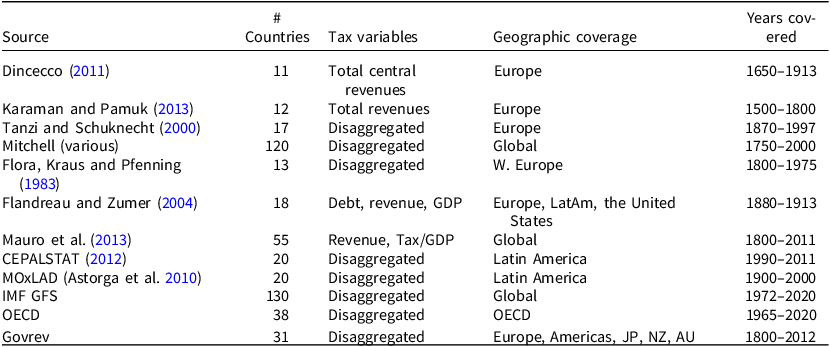
Previous research either has a long historical coverage (eg Dincecco Reference Dincecco2009) for small samples – usually Western Europe (Aidt and Jensen Reference Aidt and Jensen2013), sometimes adding English-speaking offshoots and Japan – or a wide geographic coverage only for the recent decades (eg ICTD/UNU-WIDER 2020). Historical efforts rarely provide yearly data (eg Tanzi and Schuknecht Reference Tanzi and Schuknecht2000) or present information only on the size of governments (Karaman and Pamuk Reference Karaman and Pamuk2013). This is problematic since politics is not only about the size of the state but also about who is paying for it. Indeed, the mix of taxes a state employs is often the result of fierce competition between societal groups (eg Barnes Reference Barnes2020). Table 1 provides an overview of previous efforts compared to Govrev.
Previous efforts

Note: The coverage in terms of geography, disaggregation, and time refers to the maximum. For instance, a starting year of 1750 does not mean yearly data on all countries covered, often just scattered information for one or a few countries. Many countries included in these datasets did not even exist as independent (or united) states for major parts of the period. Moreover, yearly data is rare, Tanzi and Schuknecht (Reference Tanzi and Schuknecht2000) for instance present data only once per decade or even less, totaling nine data points in time. Many of the previous efforts in the above table, for instance, Dincecco (Reference Dincecco2009), MOxLAD (Astorga et al. Reference Astorga, Berges, Fitzgerald and Rosemary2010), and Tanzi and Schuknecht (Reference Tanzi and Schuknecht2000) – as well as recent papers such as Lee and Paine (Reference Lee and Paine2023) – are based wholly or in part on Mitchell, overstating the number of sources in existence.
One tax that is not only a subject of political conflict but was also a key step in the rise of the modern fiscal state is the income tax. The wide coverage of Govrev allows comparing Europe with Latin America, two regions with different political histories and different exposure to conflict (eg the two world wars). Figure 1 shows the development of tax revenues as a share of GDP, and the income tax share in these two regions. It is interesting to note that the First World War did not coincide with increased taxation in Latin America, but the Second World War did. However, the increase in terms of tax/GDP was larger in Europe, and this divergence persists to the present day. This has implications for the relationship between war and taxation – Latin America was much less affected by the world wars than Europe – such as the so-called ‘ratchet effect’ of war finance (eg Peacock and Wiseman Reference Peacock and Wiseman1961).
Europe and Latin America compared.

Many scholars rely heavily on Mitchell (Reference Mitchell2007a, Reference Mitchell2007b, Reference Mitchell2007c), for example, Beramendi, Dincecco and Rogers (Reference Beramendi, Dincecco and Rogers2019), Cagé and Gadenne (Reference Cagé and Gadenne2018), and Lee and Paine (Reference Lee and Paine2023). We have a different approach which we believe is superior. Instead of taking databases such as Mitchell at face value, we validated sources extensively, often cross-checking with country-specific information, to find as reliable data as possible. We discovered that Mitchell is often unreliable. When comparing his information with high-quality country-specific data, we found two main causes for concern. First, Mitchell is often inconsistent in the way budget items are coded or even which parts of government budgets are presented, which causes problems when interpreting changes over time and across countries. The second problem is that the subcategories of revenues in Mitchell (eg direct and indirect taxes) at times sum to more – or significantly less – than a hundred percent, which suggests underlying issues with the aggregation process.
For instance, during the entire post-Second World War era, the sum of Danish direct and indirect tax revenues is reported by Mitchell to have been more than 100 percent. In the late 1980s and early 1990s, it exceeded 150 percent. Other examples include Uruguay, which Mitchell’s data suggest had customs revenues of more than 100 percent of total revenues in 1981 and 1982, the sum of indirect and direct taxes reaching 153 percent in 1981. In the 1930s, the Netherlands is claimed to have generated around 80–90 percent of tax revenues from direct taxes and between 40 and 50 percent from indirect taxes, which means a total of around 120–140 percent during these years. These implausible estimates suggest underlying issues in the aggregation process, for instance, revenues being counted twice, or denominator and numerator using different levels of aggregation (eg central versus general government). Other reasons may be inconsistent coding of local/central taxes, for instance, recording a local property tax in central revenues or vice versa. There may also be issues with the underlying data on which Mitchell relies.
The information in Mitchell is not only characterized by high volatility but is also often unreliable regarding levels and trends when compared to trusted sources.Footnote 6 For Denmark, we found high-quality data from Johansen (Reference Johansen1985), which we also use extensively in the final dataset.Footnote 7 Comparing this data to Mitchell reveals dramatic discrepancies. The 1918 direct tax share in Johansen is four times Mitchell’s estimate, and the discrepancies are also present in trends, with Mitchell reporting a decrease in the direct tax share around that time while the opposite is the case in Johansen. Using Mitchell would lead analysts to conclude not only that Danish direct tax revenues were small, but also that they were decreasing, while they were in fact substantial and increasing during that time. That Danish direct tax revenues were small, and decreasing in this period is unlikely also because the First World War severely disrupted international trade and thus affected customs revenues. As revenues from customs decrease, the shares from other revenues mechanically increase (if unaffected). Moreover, states that were deprived of revenues from taxes on international trade needed to make up for lost revenues by increasing domestic taxation. Finally, although Denmark did not participate in the war, it faced higher costs because of it, for instance, costs associated with mobilization and the construction of fortifications. Thus, increased direct taxes during war time is expected. Another reason to prefer Johansen over Mitchell is that in years with different sources available, the Johansen estimates are in agreement with credible sources such as the OECD, while Mitchell’s figures are not (eg excise revenues in the 1970s).
Finally, Mitchell does not cover subcategories of the budget (eg income taxes) as extensively as aggregated categories such as direct tax shares. For instance, Mitchell does not provide disaggregated data for Bolivia, Ecuador, and Paraguay. Table B.1 in the online Appendix shows the country-by-country differences in coverage between Mitchell and Govrev.
For these reasons, among others, we minimize the use of Mitchell, and when using it, we try to find ways of validating the trustworthiness of the estimates (eg by using country-specific sources). In the Govrev dataset, only one to five percent of tax category data comes from Mitchell.Footnote 8
Elite competition and taxation
The answer to how states gained the ability to tax significantly more than a few percent of GDP is (in most cases) the expansion of direct taxes. The key innovation was the modern income tax. The origins, expansion, and politics of this tax have received increasing attention, with some arguing that income tax was a tool used by the old landed elite to tax economic competition from industrialists (Mares and Queralt Reference Mares and Queralt2015), and others arguing that it was the outcome of elite competition (Beramendi, Dincecco and Rogers Reference Beramendi, Dincecco and Rogers2019 (BDR); Emmenegger, Leemann and Walter Reference Emmenegger, Leemann and Walter2021).
In this section, we use our dataset to reanalyze the findings in BDR. Their argument is that in early industrializers, fierce competition between capitalist and agricultural elites left capitalist elites (who preferred more spending on public goods) with no choice but to tax themselves through direct taxation. Why? Because (1) broad-based consumption taxes such as VAT were not technologically feasible at the time, (2) shifting taxation to the agricultural elite (eg land taxation) was not politically viable, and (3) since capitalist elites preferred a liberal trade regime, taxes on international trade were off the table. This left income tax as the only option.
In late industrializers, there was less elite competition and agricultural elites dominated. These elites may still prefer a moderate increase in spending (since some public goods increase agricultural output), but the need for new taxes was lower because of more foreign direct investments. Since this group of countries were export-oriented, taxes on international trade were off the table, and the tax mix reflected the ability of the ruling agricultural elite to finance spending through VAT, which had become feasible in this period.
Their model generates the hypotheses that elite competition is associated with (1) higher overall tax revenues and (2) a larger direct share (as a proxy for tax on capitalist elites). BDR measure elite competition in two ways, executive recruitment and political contestation. Their tax data comes predominantly from Mitchell (before 1965) and modern databases such as the OECD, IMF, and the World Bank. They cover 31 countries from 1870 to 2010.
Figure 2 compares the BDR and Govrev direct taxes estimates from 1800 to 2012. Note that BDR do not cover the first 70 years of the 19th century, during which important reforms – such as the 1842 introduction of the income tax in the United Kingdom – were implemented. BDR generally underestimate the share from direct taxes, up until 1965, when they report a sharp increase. This increase is due to BDR switching main source from Mitchell – which records the share of direct taxes at central government level – to the OECD data on general government level (ie including local and regional levels).Footnote 9 Govrev consistently presents central-level information and reports no jump in 1965 (despite making extensive use of the OECD as a source). In Table C.1 of the online Appendix, we study this jump in detail using the case of Belgium.Footnote 10 The table shows how the discrepancy is created by BDR switching from Mitchell – which records revenues on the central level – to the OECD total/general revenues series. The OECD data make clear that the differences are due to the size of revenues from social security contributions: around 2 percent of central tax revenues, but around 30 percent of total revenues.Footnote 11
Direct tax share. The BDR and Govrev estimates of the average share of total central tax revenues from direct taxes over time.

The divergences around the First World War are likely due to both coding choices and differences between Mitchell and Govrev. First, BDR sometimes seem to replace missing values with 0, and at other times they report a direct share of 0 even though Mitchell reports other estimates (eg Norway).Footnote 12 Second, in many cases, Mitchell reports much lower figures for the direct share compared with Govrev (eg Portugal). Table D.1 in the online Appendix compares the three sources during the First World War and shows that the Govrev estimates are often higher than both BDR and Mitchell (eg New Zealand, Peru, and Sweden).
These issues with the underlying data may affect the conclusions we draw from analyzing the rise of direct taxation. The following replication exercise uses five-year averaged data with the direct share as dependent variable, following Table 2 in BDR.Footnote 13 In Table 2, we present first the replicated BDR results using the original BDR sample (‘OS’), then the results using the common sample between Govrev and BDR (‘CS’), and finally the results using Govrev data on the common sample. The upper panel presents results without controls (but with fixed effects for time and country, following BDR) and the lower panel results with controls. The controls (all lagged) are war mobilization, GDP/capita, left-wing head of government, tax/GDP, lagged dependent variable, and region-specific time trends.Footnote 14 Standard errors are clustered at the country level.
Reanalysis of Table 2 in BDR. Dependent variable: direct tax share

Five-year averaged data. Dependent variable: direct tax share. All regressions include country and period fixed effects. The lower panel includes control variables and region-specific time trends. OS = original sample; CS = common sample. Robust standard errors clustered at country level are in parentheses. *p < 0.10; **p < 0.05; ***p < 0.01.
Restricting the sample to observations covered by both datasets, we are able to reproduce the results for both executive recruitment and political contestation using BDR’s data as long as no controls are included. Using the Govrev data, the coefficients of interest are insignificant (although political contestation is significant on the 10% level). Once we use the more stringent specifications (lower panel), only the results for executive recruitment can be replicated using BDR’s data. The coefficient for executive recruitment is virtually identical and statistically significant (column 2, second panel). However, using Govrev the coefficient is much weaker and statistically insignificant.Footnote 15 It is interesting to note that the standard errors are comparable and that the model fit is not radically different, with R2 (within and adjusted) somewhat higher when using the BDR data while the RMSE is lower when using Govrev.Footnote 16
To investigate whether these differences result from measurement issues, we scrutinize influential observations indicated by DFBETAs (Figure F.1 in the online Appendix).Footnote 17 While there is variation, on average these observations increase the strength of the hypothesized positive relationship between executive recruitment and direct tax share.
By analyzing these observations more closely, we see that BDR often provide implausible estimates compared to Govrev, both in levels and trend. For instance, in Japan in 1941, BDR report a direct tax share of 8.6 percent – implausibly low for war time – while the Govrev estimate – based on information from the Japanese Ministry of Finance – is 63 percent. It is also common with extreme volatility in the BDR data, with estimates changing dramatically year to year (eg the observations from Finland). In section F of the online Appendix, we provide more examples of how the influential observations suggest issues in the underlying data.
Further analysis
In this section, we use Govrev to further explore the empirical implications of BDR’s theory. Specifically, BDR clearly differentiate between direct taxes affecting the agricultural elite – land taxes – and direct taxes hurting the capitalist elite – income taxes. However, their measure – ‘direct taxation’ – includes both of these. Thus, an insignificant coefficient may be caused by elite competition leading to higher income taxes but lower property taxes, which would not be inconsistent with BDR’s argument. In the analysis below, we use the more detailed data in Govrev to explore the possibility that elite competition is linked to differences within direct taxation. A second implication in BDR (which is tested using the sum of all indirect taxes in their online Appendix) is that low elite competition should be linked to greater revenues from VATs. Using Govrev, it is possible to distinguish broad-based consumption taxes such as VATs from specific taxes on goods and services (excises) and from taxes on international trade.
The results in Table 3 reveal that elite competition is associated with lower income taxes and higher excise taxes, suggesting capitalist elites avoided taxing themselves and pushed taxation onto other groups. However, there is no link between low elite competition and higher consumption taxes, something BDR expect to find, but high elite competition is related to more excise revenue. In line with BDR’s expectations, property taxes are not linked to elite competition. These results suggest that elite competition is associated with taxes being shifted from urban elites to the urban working class (ie from a more progressive to a more regressive tax mix).
Decomposing direct revenue

Five-year averaged data. All models include a full battery of controls, country and period fixed effects, and a lagged dependent variable. Robust standard errors clustered at country level are in parentheses. *p < 0.10; **p < 0.05; ***p < 0.01.
These findings indicate that more elite competition means higher taxes for the non-elite. However, given that elite competition is measured as executive recruitment and political contestation, there are more straightforward explanations from the existing literature. First, that intense political competition is associated with a decrease of (visible) taxation – such as income tax – and increased taxes on commodities (excises) aligns with the findings in Aidt and Eterovic (Reference Aidt and Eterovic2011). Thus, if the elite competition variables pick up changes in political competition – which is likely in this case – the results can be explained by their suggested mechanism.
Insofar as the indicator captures the increasing power of the modern urban elite, the results are in line with the argument that income tax is used by the old landed elite to check the economic power of the modern industrial elite (Mares and Queralt Reference Mares and Queralt2015). Thus when the capitalist elite become more powerful, they help reduce taxes on income. In essence, the tax mix reflects the groups in power.
The failure to replicate the key results in BDR, and the findings in the extended analysis, suggest that elite competition theory needs to be refined. For instance, the landed elite may invest in the industrialized sector (which they did in, eg Sweden; see Bengtsson and Olsson (Reference Bengtsson and Olsson2020)) and thus share the tax preferences of the capitalist elite. We also know from existing research that the history of the income tax is more autocratic than democratic, encouraging us to consider alternative explanations, such as coalitional dynamics and voting rights conditional on tax payments (Mares and Queralt Reference Mares and Queralt2020), or how legislative oversight facilitates fiscal capacity in non-democratic states (Andersson Reference Andersson2023).
Conclusion
In 2015, Hoffman (Reference Hoffman2015) lamented the paucity of historical tax revenue data, identifying it as a major obstacle in several research areas. In this paper, we have presented a first attempt to solve this problem.
Covering a larger sample, a longer time period, and providing more detailed information than previous efforts, the Govrev dataset allows scholars to better test existing theories and uncover new patterns. As an example, we demonstrated that the relationship between elite competition and fiscal outcomes differs from previous findings. We find that, historically, the capitalist elite shifted taxation onto the poor. While this supports parts of BDR’s theory – the new elite did not tax the agricultural elite – it does not support the main idea that the new elite taxed themselves.
While our contribution takes us some of the way, much remains to be done. For instance, there is a need to expand the sample in space – by including, for example, China, Russia, and Ethiopia – and in time, by collecting pre-1800 revenue data. Further work is also needed to get a complete picture of taxation also at the local and regional level which, in many countries, is substantial. Including local and regional levels would increase the comparability between federal and unitary states. As more historical sources become available, it will also be possible to improve on the existing estimates.
Supplementary material
The supplementary material for this article can be found at https://doi.org/10.1017/S1475676526100929
Data availability statement
Data and replication files are available at perfandersson.com/data and at the Harvard Dataverse: https://doi.org/10.7910/DVN/P1VAGP.
Acknowledgments
I wish to thank Jan Teorell, Jacob Gerner Hariri, two anonymous reviewers, and the editor of the EJPR for comments and advice. All errors remain my own.
Funding statement
I acknowledge generous support from the Swedish Research Council (grant no. 2023-01580).
Competing interests
The author reports none.


 Open access