2. Related work

The vast majority of FRBs have been detected using beamforming techniques and dedicated compute infrastructure (Amiri et al. Reference Amiri2021). The CHIME/FRB collaboration established an FRB detection system that upgrades the GPU correlator of the CHIME telescope to produce 16 384 fine channels at 1 ms time resolution. The correlation software runs on 256 dedicated processing nodes, each with two commercial dual-chip AMD GPUs. The output is fed to a beamforming pipeline creating 1 024 beams across the sky, then passed to further stages for detection and classification of FRBs (Amiri et al. Reference Amiri2018).

However, imaging is emerging as an alternative method to recover the sky intensity over time and frequency. The ASKAP’s CRAFT project presented the CRAFT COherent upgrade (CRACO), an FRB search system based on millisecond-scale imaging implemented on 22 FPGA boards. By forming 256 $\times$ 256 images covering 1.1 square degrees of sky, their goal is to obtain precise localisation of detected FRB events (Wang et al. Reference Wang2025).

Observations taken with the MWA have been searched several times for FRBs (Tingay et al. Reference Tingay2015; Rowlinson et al. Reference Rowlinson2016; Sokolowski et al. Reference Sokolowski2018; Kemp et al. Reference Kemp, Tingay, Midgley and Mitchell2024) using imaging-based techniques. For instance, the MWA was used to shadow the ASKAP telescope by recording and imaging visibilities at 0.5 s time and 1.28 MHz frequency resolutions. While ASKAP detected FRB pulses, no low-frequency counterparts were found (Sokolowski et al. Reference Sokolowski2018). If bright enough FRBs were indeed recorded by the MWA, likely reasons for null results would be coarse integration times, in the scale of seconds, insufficient hours of observations analysed based on the expected FRB rate (Sokolowski et al. Reference Sokolowski2024a), or both.

All MWA imaging pipelines are a sequence of established radio astronomy packages whose execution is orchestrated using BASH or Nexflow. COTTER (Offringa et al. Reference Offringa2015) handles visibilities correction and data format conversion from FITS to MeasurementSet; AOFlagger applies RFI mitigation; WSClean (Offringa et al. Reference Offringa2014), Miriad or CASA are adopted for gridding and imaging. Each step in the pipeline reads in from the filesystem the previous step’s output and produces files to be given as input to the next one. An in-depth description of a representative MWA imaging pipeline is given in Section 5.

Except for Kemp et al. (Reference Kemp, Tingay, Midgley and Mitchell2024), none of the highlighted MWA publications mentions the computational setup and costs of running such searches. In the latest search for FRBs within more than one hundred hours of MWA observations, Kemp et al. (Reference Kemp, Tingay, Midgley and Mitchell2024) underline the importance of parallel processing and scalability to reduce compute time by taking advantage of supercomputing infrastructure. In their approach multiple 2-min observations are distributed across and independently imaged at 2 s resolution by 64-core CPU nodes of a commercial cluster. The Input/Output (I/O) bottleneck afflicting established MWA processing software is addressed by mounting RAM as a filesystem where intermediate files are written to and read from. By doing so, they managed to process 400, 2-min observations in 25 min.

The first GPU implementation of voltage correlation was presented by Harris, Haines, & Staveley-Smith (Reference Harris, Haines and Staveley-Smith2008), a work which demonstrated its feasibility and computational advantage over a CPU implementation. The research fed into a first GPU correlation system developed for the MWA prototype (Wayth, Greenhill, & Briggs Reference Wayth, Greenhill and Briggs2009) as well as into the highly optimised xGPU correlation library (Clark, La Plante, & Greenhill Reference Clark, La Plante and Greenhill2011). The latter has been subsequently adopted for the MWA online correlation system (Ord et al. Reference Ord2015; Morrison et al. Reference Morrison2023). Romein (Reference Romein2021) presented a GPU correlator that leverages the NVIDIA Tensor Cores to achieve up to 10x speed up compared to xGPU. The idea of an imaging pipeline for the MWA taking advantage of the computational power of GPUs is not new (Ord et al. Reference Ord, Greenhill, Wayth, Mitchell, Dale, Pfister and Edgar2009), but has not effectively taken over the established workflows mostly based on CPU software. GPU acceleration is only routinely used through the Image Domain Gridder (IDG) software (Veenboer et al. Reference Veenboer, Petschow, van der Tol and Offringa2019), part of the popular WSClean imaging application.

RICK is a GPU software with a similar philosophy to BLINK but a different objective (De Rubeis et al. Reference De Rubeis, Lacopo, Gheller, Tornatore and Taffoni2025). It is a library of imaging routines developed to run on HPC environments with MPI support and NVIDIA GPU acceleration. They focus on the processing of LOFAR massive visibilities datasets to produce large images, of the order of 500 GB and 65K $\times$ 65K resolution, respectively.

The BLINK GPU imager is a software designed to execute visibilities corrections, gridding, and FFT, making up the later part of the imaging process, entirely on GPU, supporting both NVIDIA and AMD vendors (Sokolowski et al. Reference Sokolowski, Aniruddha, Di Pietrantonio, Harris, Price and McSweeney2024b). It specifically targets the scientific goal of finding FRBs and hence focusing on meeting the demanding computational requirements imposed by high time and frequency resolutions, and a large FoV. The BLINK GPU imager is a component of the BLINK imaging pipeline presented in this work, and the BLINK FRB search pipeline, to be implemented in the future.

3. Motivation

A summary of representative science requirements imposed on FRB searches with the MWA is presented in Table 1, informed by the telescope specifications and other FRB searches in similar settings (Pleunis et al. Reference Pleunis2021; Gopinath et al. Reference Gopinath2023). FRBs are subject to large DM and accentuated dispersion at low-frequencies, meaning that tens of seconds must be considered when constructing dynamic spectra. The dispersive delay is three orders of magnitude larger than the integration time. This results in more than half a million of images, which occupy at least 0.5 TiB of memory, being manipulated roughly at any given time during the processing.

Then, processing tens of hours worth of observations in a timely and efficient way requires more computational power, measured in FLoating-point OPerations per Second (FLOPS), than a single workstation or a small cluster can provide. The new Setonix supercomputer (Hewlett-Packard Enterprise 2022), hosted at the Pawsey Supercomputing Research Centre, provides a partition of GPU nodes comprising 768 AMD MI250X GPUs that reaches approximately 35 PFLOPS, representing the majority of compute provided by the entire system. In fact, nearly all the newly-procured supercomputers derive most of their compute power from GPU accelerators (Feldman Reference Feldman2018) due to their computational speed and energy efficiency.

Table 1.

Representative requirements and constraints for an FRB search with the MWA. The high time and frequency resolution requirements, the large instantaneous bandwidth of the MWA, and the dispersive delay causing the signal to cross the low frequency band in tens of seconds demand the FRB search software to handle half a million of images per each time frame needed to compute dynamic spectra.

However, the vast majority of radio astronomy software developed by researchers is designed to run in isolation on CPU-only workstations or small clusters at most. Only a small subset of established and widespread software leverage GPUs, and they target NVIDIA ones, making the majority of Setonix compute power inaccessible to these applications. Furthermore, even when GPUs are used, the extensive reliance on the filesystem to store intermediate data products considerably slows down the processing. In recent years, radio astronomers and developers have started addressing the aforementioned issues but have not converged to a solution yet (Edgar et al. Reference Edgar, Clark, Dale, Mitchell, Ord, Wayth, Pfister and Greenhill2010; Mitchell et al. Reference Mitchell, Greenhill, Wayth, Sault, Lonsdale, Cappallo, Morales and Ord2008; Law et al. Reference Law2018).

The BLINK imaging pipeline is a new radio astronomy software written with the primary goal of running large scale FRB searches in the MWA archival data. All computations are executed on GPU and intermediate data products reside in GPU memory, removing unnecessary I/O operations. The software is written to support both NVIDIA and AMD GPUs. While the BLINK imaging pipeline has been successfully tested on an NVIDIA cluster, it is mainly developed on the Setonix GPU partition, its target execution environment. By using Setonix, a large number of observations can be processed in parallel over multiple GPUs and compute nodes, drastically increasing the FLOPS available to the computation.

4. The imaging process

Interferometers feature a large number $N_a$ of independent antennas spread over a significant surface area. Each antenna records time series $V_a(t)$ of voltage data describing radiation coming from a range of frequencies and from all directions within the antenna beam, corresponding to the FoV. There are different ways of combining these signals into a robust source of information. In coherent beamforming, signals are coherently added together to form a voltage beam b(t):

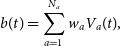(1) \begin{equation} b(t) = \sum_{a = 1}^{N_a} w_a V_a(t),\end{equation}

where $w_a$ is a per-antenna correction term used to phase signals to point towards a specific direction in the sky. The power beam B is obtained by squaring and averaging in time:

(2) \begin{equation} B = \left\langle b(t) b^*(t) \right\rangle. \end{equation}

The computational time complexity of beamforming the entire FoV is $\Theta(N_a N_x^2)$ , where $N_x = B_{max} / D$ , $B_{max}$ is the maximum distance between antennas, and D is the diameter of an antenna aperture.

As the angular resolution and FoV of modern radio telescopes increase, beamforming becomes computationally prohibitive. Imaging is a viable alternative to analyse data from low-frequency radio telescopes such as the MWA and Low Frequency Square Kilometre Array (Labate et al. Reference Labate, Waterson, Alachkar, Hendre, Lewis, Bartolini and Dewdney2022), although still very computationally expensive.

In the interferometric imaging process (Condon & Ransom Reference Condon and Ransom2016), The first step is to construct the cross power spectrum by multiplying fine-channelised voltages from each pair of antennas $(a_i, a_j)$ , and averaging the result in time (Ord et al. Reference Ord2015):

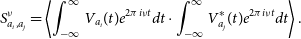(3) \begin{equation} S^\nu_{a_i, a_j} = \left\langle \int_{-\infty}^{\infty} V_{a_i} (t) e^{2\pi i\nu t} dt \cdot \int_{-\infty}^{\infty} V^*_{a_j} (t) e^{2\pi i\nu t} dt \right\rangle.\end{equation}

The fine channelisation has a cost of $\Theta(N_aF\log_2F)$ and the multiplication is done in $\Theta(N_a^2)$ operations.

The cross power spectrum $S^\nu_{a_i, a_j}$ measures a finite sample of the spatial frequency space $S^\nu(u, v)$ of the radio signal, also called visibility function. Let (u, v) be the coordinates in such space, and (l, m) the direction cosines of sky pointings. Then, visibilities are related to the sky brightness distribution by the following approximation:

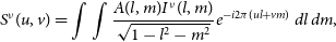(4) \begin{equation} S^\nu(u, v) = \int\int \frac{A(l, m) I^\nu(l, m)}{\sqrt{1 - l^2 -m^2}}e^{-i2\pi(ul + vm)}\, dl \, dm,\end{equation}

where A(l, m) is the primary beam of the telescope, and $I^\nu(l, m)$ is the sky specific intensity one wishes to measure. Equation (4) defines the visibility function as Fourier transform of the sky intensity.

Samples in $S^\nu_{a_i, a_j}$ are placed on a regular grid $S^\nu(u_x, v_y)$ whose side turns out to be of length $N_x$ , in a process called gridding. Then, the 2D inverse Fast Fourier Transform (2D FFT) algorithm is used to recover an approximation of $I^\nu(l, m)$ , the dirty image $\hat{I}^\nu(l, m)$ :

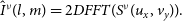(5) \begin{equation} \hat{I}^\nu(l, m) = 2D FFT(S^\nu(u_x, v_y)).\end{equation}

It is an approximation because the finite number of antenna pairs does not provide full coverage of the (u, v) plane. The computational time complexity of gridding is $\Theta(N_a^2)$ , and the 2D FFT one is equal to $\Theta(N^2_x\log(N^2_x))$ .

Most science applications of imaging require a further step named deconvolution, where artifacts due to the discrete sampling of the (u, v) plane are removed from the dirty image. CLEAN (Högbom Reference Högbom1974) is an iterative algorithm that implements deconvolution and it is computationally expensive to run. However, FRBs are so bright that such distortion effects do not practically impair the detection process and the CLEAN step is not necessary. For the same reason, we do not correct distortions caused by the wide FoV.

Correlation and inverse 2D FFT are the most computationally expensive steps of the dirty imaging process. Assuming the image side length $N_x$ is greater than the number of antennas $N_a$ , the execution of the correlation algorithm is likely to be faster than the 2D FFT one. However, the former is performed at every time sample whereas the latter only at the end of an integration interval containing $N_s$ time samples. The cost of the 2D FFT per time sample is $\Theta(N^2_x\log(N^2_x)N_s^{-1})$ . Figure 1 illustrates the contribution of correlation, gridding and 2D FFT to the total execution time of the imaging process as a function of the integration time. Figure 2 shows that correlation and 2D FFT are almost equally important for a representative integration time required to study FRBs.

Figure 1.

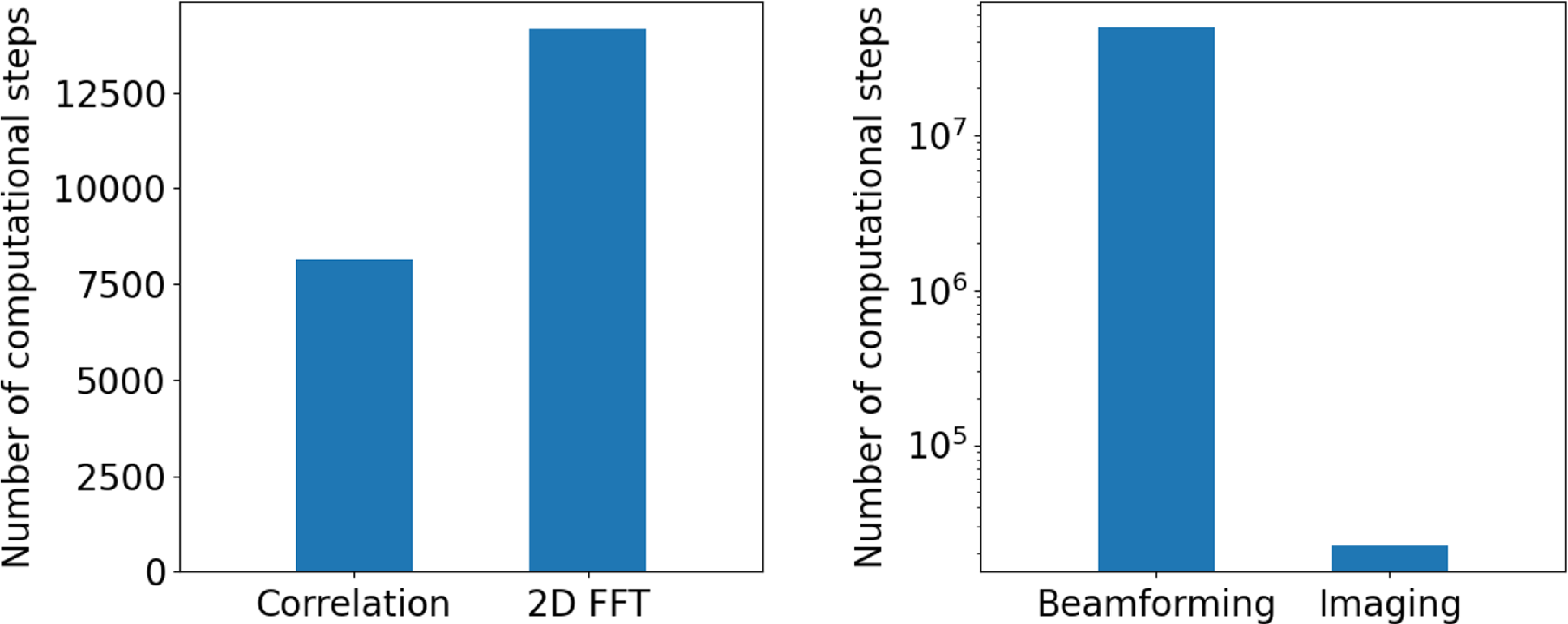
Relative computational cost per time sample of the main steps of the imaging process. The number of fundamental numerical operations of the correlation, gridding and 2D FFT algorithms expressed as a percentage of their sum is a proxy of their relative computational cost. Curves shown in the plot arise when the imaging process is instantiated on MWA Phase I VCS data at observational frequency of 150 MHz. The integration time is the critical parameter that determines whether 2D FFT or correlation is the dominant part of the computation.

Figure 2.

Significant computational costs in the context of an FRB search. The computational cost per time sample of correlation and 2D FFT in the imaging process for the MWA Phase I VCS data, at an integration time of 50 ms and observational frequency of 150 MHz (left panel). In the same setting, beamforming requires three orders of magnitude more computation than imaging (right panel).

Figure 3.

The BLINK FRB search pipeline. The distinguishing features of the BLINK pipeline are the utilisation of GPU cores to execute every compute stage and a homogenous data representation throughout. In addition to parallelisation of computation, the proposed approach eliminates the need of using the filesystem as a temporary staging storage. Intermediate data products to feed successive stages already reside in GPU memory, removing expensive CPU-GPU memory transfers. The CPU is left the task of reading the voltage data from disk, planning and submitting GPU computations, managing memory, and presenting the final output to the user. Dashed lines characterise steps yet to be implemented.

The reason for choosing imaging over beamforming is the computational cost. If correlation can be, within a constant factor, considered as representative of the cost of the imaging process, then the ratio between beamforming and imaging costs is $\Theta(N^2_x / N_a)$ . Because the number of pixels is at least three orders of magnitude larger and increases much faster than the number of antennas, the growth of the ratio highlights the expensive cost of beamforming. The advantage of imaging can also be found with a more precise analysis on the number of computational steps that considers the time complexity of correlation and 2D FFT, presented in the right panel of Figure 2.

5. Traditional MWA imaging pipeline

The imaging pipeline described by Sett et al. (Reference Sett, Bhat, Sokolowski and Lenc2023) is a representative example of how MWA observations are traditionally imaged. Because authors in the referenced paper use it to analyse the SMART survey (Bhat et al. Reference Bhat2023a; Bhat et al. Reference Bhat2023b), we will refer to it as the SMART pipeline. It starts by correlating voltages captured by the MWA VCS using the offline correlator program. The resulting visibilities are saved in FITS files, one for each coarse channel. Internally, offline correlator uses the GPU-accelerated xGPU library. While still retaining high performance on modern NVIDIA GPUs, xGPU was developed more than ten years ago, and it has not been maintained for six. The code contains extensive low-level optimisation logic that makes any porting to AMD GPUs unfeasible. There is another practical limitation in using xGPU: parameters such as integration time and number of antennas must be chosen at compile time. Multiple xGPU deployments are required for observations taken with different configurations of the MWA, introducing a significant administrative overhead.

Before they can be processed into science-ready data products, visibility data are corrected for instrumental and environmental effects by application of calibration, and radio frequency interference (RFI) by flagging. This is partially accomplished by multiplying each visibility point by a calibration solution that is determined using a reference object in the sky observed before or after the main observation. Other corrections involve applying a phase shift to the signal to digitally steer the telescope. These operations collectively form the preprocessing step and they are implemented in the purpose-built software COTTER. It interleaves I/O and computation, and speeds up the whole execution using CPU multi-threading. While these corrections are applied relatively quickly, most of the time is spent in I/O. The corrected visibilities are stored on the filesystem using the CASA MeasurementSet format.

WSClean is the standard software used to image visibilities. It implements a wide variety of functionalities and it is named after its implementation of the w-stacking technique to image wide FoVs, and its CLEAN implementation. For the purpose of an image-based FRB search, only the gridding and the 2D FFT are needed to produce dirty images. Within gridding, visibilities are convolved with a gridding kernel to reduce aliasing effects of out-of-FoV sources. The architecture of WSClean relies extensively on the CASA library, and in particular the MeasurementSet class to read input visibilities, to hold data through the various computational steps, and to write the resulting images back to disk. The computation takes place mainly on CPU. The gridding step is sped up with GPU acceleration through the Image Domain Gridder (IDG) plug-in module.

Automation in this setting is achieved by scripting invoking the offline correlator, COTTER, and WSClean programs for each second of the observation. The output are multiple MeasurementSet directories and FITS files representing intermediate and final data products.

6. BLINK pipeline implementation

This paper introduces the Breakthrough Low-latency Imaging with Next-generation Kernels (BLINK) pipeline to efficiently image voltage capture data in high time and frequency resolution. It will make up the first half of a larger pipeline designed to look for low-frequency FRBs within MWA observations. The code repositories for the BLINK project are publicly available on GitHub at the following link: https://github.com/PaCER-BLINK-Project.

6.3. Running the pipeline

The BLINK project makes available a command-line interface executable to run the pipeline described in this paper, aptly named blink_pipeline. It takes as input a list of .dat files representing one or more seconds of a single MWA VCS observation, and several options to set parameters such as time resolution, fine channel bandwidth, image size, and calibration solutions. The returned output currently consists of FITS files containing an image for each frequency channel and integration interval. Ultimately, the resulting image cubes will be searched for FRBs.

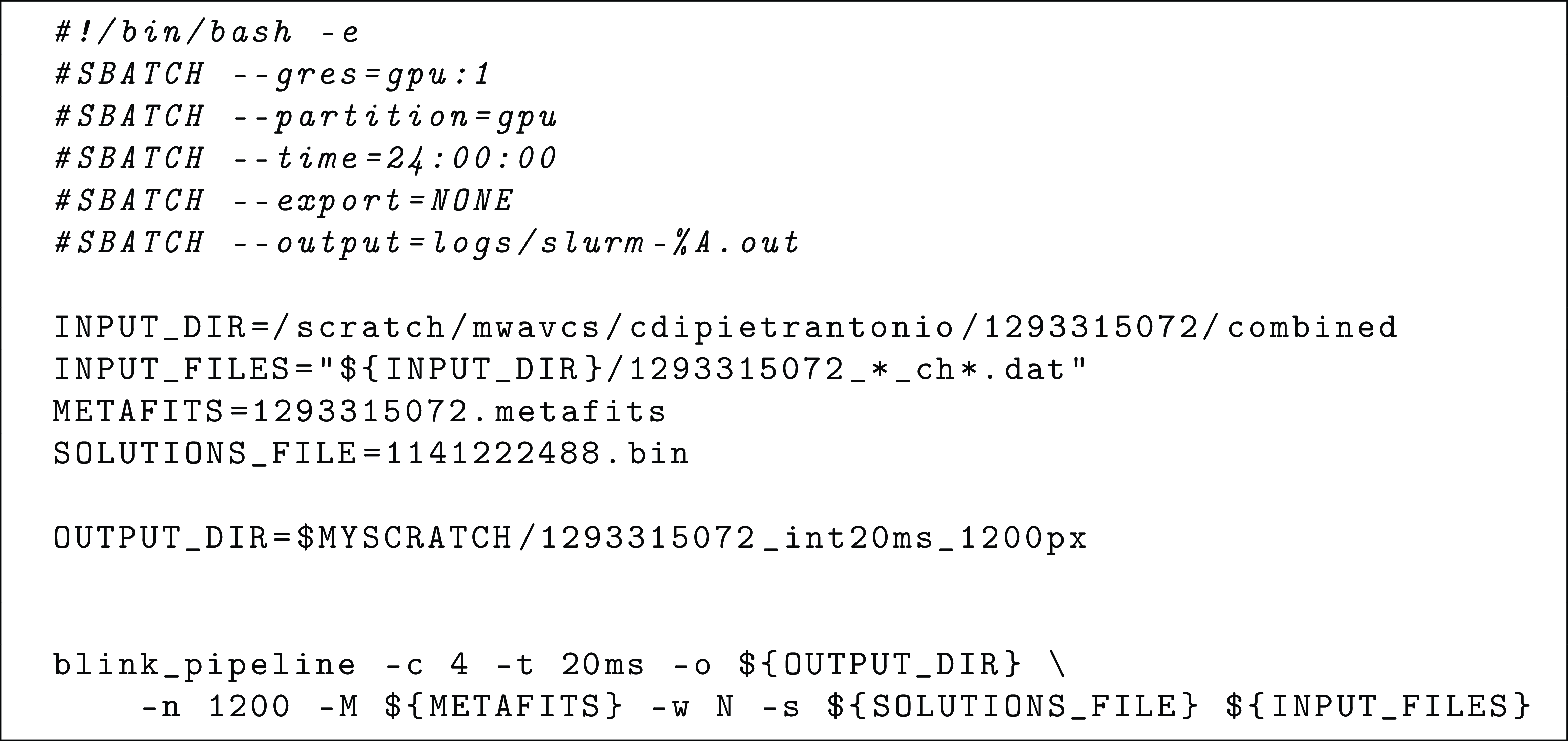
A single executable implementing the entire pipeline also provides a an intuitive interface for researchers to use. An example of submitting a BLINK imaging job to Setonix is shown in Listing 6. In contrast, established MWA imaging pipelines are made up of several BASH or Nextflow scripts chaining together a number of executable programs, each with its own input and output formats, and a wide range of command line options. The ease of use of the BLINK pipeline reduces the human time required to setup the computation, minimises configuration errors, script development time, and improves accessibility to beginners in the field.

Listing 1.

Example submission script. Executing the BLINK pipeline on the Setonix supercomputer requires minimal BASH scripting. First, Slurm directives inform the scheduler of the computational resources required to run the program. In this case, a single GPU on a node in the gpu partition. BASH variables are then defined to point to input files like observation metadata, calibration solutions, and voltage files. BASH wildcards are used to select the interval of seconds and frequency channels to process. In this case, all the data associated with OBSID 1293315072. Finally, the BLINK pipeline is executed with a single command line. Important options are: -t, the integration time; -c, the number of contiguous fine channels to average; -n, the side size in pixels of the output images.

7. Testing

Firstly, the BLINK imaging pipeline must produce reasonable dirty images of the radio sky to prove the overall correctness of the software. Secondly, it has to generate millisecond time resolution images with enough sensitivity to detect bright transients. The first objective is ensured by implementing unit tests for all major functions and classes. Low-level components are tested with synthetic data while the output of major computational routines, such as correlation and gridding, are compared to the output produced by the corresponding procedures in the reference software, the SMART imaging pipeline. Finally, the ability to detect bright pulses is tested by imaging in 20 ms time resolution few seconds of a MWA observation containing a known pulsar.

7.1. Testing environment

Experiments have been run on two Pawsey supercomputing systems, Garrawarla and Setonix, and an internal CSIRO cluster named Virga. The first one was a cluster with 78 nodes, each providing one NVIDIA Tesla V100 32GB GPU, two Intel Xeon Gold 6230 20-core CPUs, and 384 GB of memory, for a total compute capacity of 0.7 PFLOPS. Garrawarla was a system dedicated to radio astronomers and was decommissioned at the beginning of 2025. Setonix is the new Pawsey supercomputer dedicated to general research, and replaced Garrawarla as supporting system for radio astronomy research.

Setonix GPU partition contains 192 nodes, each with four AMD MI250X GPUs, a AMD Trento 64-core CPU, and 256 GB of host memory. The Trento CPU delivers 2.51 TFLOPS consuming up to 280 W of power. Each MI250X GPU is made of two Graphics Compute Dies (GCDs) seen by the runtime as two separate GPUs. A MI250X has a total of 47.9 TFLOPS peak compute capacity and Thermal Design Power (TDP) of 500 W.

Table 2.

Observation 1. Information summary of the MWA observation imaged in a long exposure setting with the BLINK and SMART pipelines.

At the time experiments were executed, both Garrawarla and Setonix mounted the same /scratch Lustre filesystem. Furthermore, GPU nodes of both systems have a local NVMe disk processes can use for fast I/O. In these experiments, input data is always read from /scratch. Output images are written to either the Lustre filesystem or the NVMe disk depending on the volume of data produced.

For both test cases the SMART pipeline was run on Garrawarla because the offline correlator requires NVIDIA CUDA, whereas the BLINK pipeline was executed on Setonix GPU nodes. While the latter can be compiled for an NVIDIA system, the current prototype targets MI250X specifications and demands GPUs with more than 32 GB of memory to store high time resolution images, as shown in Table 7. In the future, Managed Memory, currently adopted to ease the ingest of voltage data, might be implemented throughout the pipeline to ease GPU memory restrictions. Then, the two pipelines run on different hardware, and in a different modality. The SMART pipeline makes heavy use of CPU cores whereas BLINK only uses CPU to read in data and to orchestrate GPU computation.

To abstract away these differences in parts of the discussion, we define the concept of execution unit as the minimal hardware requirements to execute an imaging pipeline. On Garrawarla, it is an entire GPU node. On Setonix, it corresponds to a single MI250X GCD and 8 CPU cores, or $1/8^\mathrm{th}$ of a GPU node. Each instance of a pipeline is allocated an execution unit to process one or more seconds of observation sequentially. An observation can be partitioned in batches of seconds which are processed in parallel over multiple execution units.

This work focuses on the novel software architecture adopted by BLINK. However, to support the claim that the software supports both NVIDIA and AMD GPUs, in the second test case BLINK was also run on the Virga cluster after Garrawarla had been decommissioned. Virga is a GPU cluster featuring NVIDIA H100 GPUs.

Figure 4.

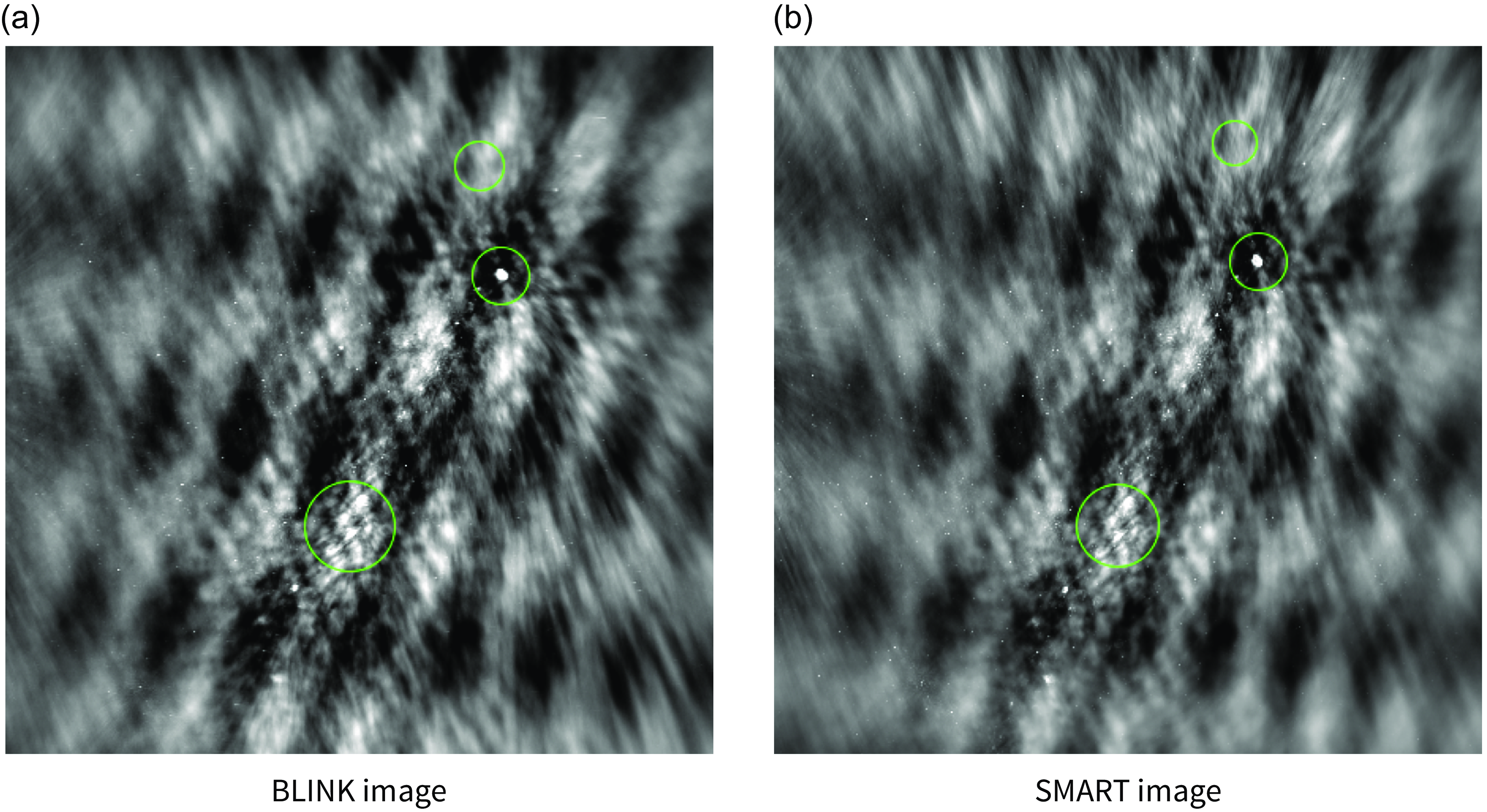
Long exposure images. The BLINK and SMART pipelines were run on the MWA Phase II Extended 1276619416 observation in multi-frequency synthesis mode, averaging images across all time bins, which resulted in the long exposure images shown in these panels. Three regions are highlighted by green circles in both images to compute key statistics for the purpose of comparison. These are reported in Table 3.

7.3. High time resolution images

The second test consists in the generation of high time resolution images of MWA OBSID1293315072, details in Table 4, to detect the pulses of PSR B0950+08. A single radio emission from a pulsar is the closest resembling transient event to an FRB that has been recorded with the MWA, and its detection would provide great confidence that the presented pipeline is sensitive to millisecond radio transients.

The BLINK pipeline has been run on the first seven seconds worth of VCS data by correlating voltages at 20 ms time and 40 kHz frequency resolutions. This configuration results in 50 time bins and 768 fine channels. Visibilities from each frequency channel and time bin are gridded in parallel on separate grids. The process produces 38 400 images of chosen resolution 1200 × 1200 pixels per second of observation, then written to a node-local NVMe volume for visual inspection. Images belonging to the same time bin are averaged together, effectively covering the whole 30.75 MHz frequency bandwidth of the MWA. The dispersive delay affecting the signal is almost negligible because the DM is only 2.97, and the de-dispersion is not applied to simplify this demonstrative analysis.

Table 3.

Key image statistics. This table reports key statistics of the three regions highlighted in the long exposure images produced by the BLINK and SMART pipelines. The top region does not contain any source and it is ideal to sample the noise level. The two other regions contain extended objects, providing opportunity to compare peak fluxes.

Table 4.

Observation 2. Details of the MWA observation that has been imaged at 20 ms time resolution with the BLINK imager.

The radio pulse of PSR B0950+08 is clearly visible in the image sequence, a sample of which is shown in Figure 5. Visibilities are not phase-centred at the location of the pulsar, then seen in the middle-left part of the FoV and highlighted by a red circle in the images. Each column depicts an independent pulse detection. Images in the centre row capture the peak of pulses, whereas the first and third show the sky intensity moments before and after those. The noise level sits at 0.5 Jy, which is in good agreement with the expected value based on electro-magnetic simulations. The two brightest pulses have a flux density of 9 and 16.5 Jy.

We attempted to run the SMART pipeline in an equivalent configuration but WSClean could only generate 2 730 of the 38 400 images within the 24 h wall time imposed on Pawsey supercomputing systems. This implies an execution time that is too long for WSClean to efficiently image multiple frequency channels and time intervals over entire observations.

Figure 5.

High time resolution images. The figure shows a sample of the 20 ms images generated with the BLINK pipeline as part of the second test case. These contain bright pulses of pulsar B0950+08, whose position is marked with a red circle. The centre row shows the images with bright single pulses at UNIX times 1609279857.740 (left column) and 1609279856.480 (right column). The 20 ms images before and after the pulses are respectively in the rows above and below the centre one. When the peak of the pulse is closer to the edges of time bins its residual signal appears in the before and after images. The average noise in the images is equal to 0.5 Jy. The two brightest pulses have a flux density of 9 and 16.5 Jy.

8. Benchmarking

The computational performance of the BLINK pipeline against the SMART one is evaluated in terms of execution time needed to process one second of full-bandwidth observation given a single execution unit as defined in Section 7.1. We report the timings for both test cases although it is the second test that is representative of the compute requirements of the target science case. Timings of the imaging stages are recorded for each second of observation processed. However, for the SMART pipeline it was not possible to distinguish between time spent in I/O and computation at each stage due to the fact these operations interleave. In the BLINK pipeline input ingestion occurs at the beginning before any computation starts. We also report the time it takes to write out the final images, for completeness. That last operation will not be required when the pipeline will be extended to support FRB searches.

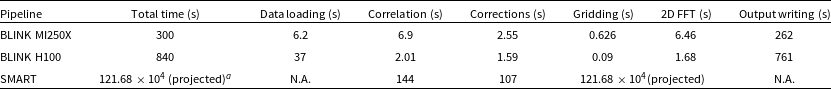
Test case one processed 4 660 s of observation partitioned in batches of 100, each batch submitted as an independent computation to the supercomputer. Timings recorded for each second are averaged and reported in Table 5. On average, the BLINK pipeline is 3.8 times faster than the SMART one, with mean total execution times, respectively, of 48.75 and 184 seconds. Close to 95% of the BLINK execution time is spent in reading input files and writing out images, operations whose distribution of timings is characterised by a significant standard deviation. While we could not directly quantify it, I/O activities impact the SMART pipeline as demonstrated by the mean execution time and the standard deviation of the corrections step. This is implemented by the COTTER program that writes its output as a CASA MeasurementSet. It has been experimentally observed that writing data to such format incurs in degraded performance on Pawsey’s /scratch Lustre filesystem, mainly due to the large number of requests to metadata servers. The contribution to the total execution time of the computational kernel is minimal in comparison. Hence, the GPU acceleration provides little improvement in this mode of operation.

Table 5.

Execution times for the long exposure images. Execution times and their standard deviation (in brackets) of the various phases of the SMART and BLINK imaging pipelines needed to process one second of observation at 1 s time resolution and 40 kHz frequency resolution. Values are an average over 4 660 s worth of observation. For the SMART pipeline, timings for the Data loading and Output writing are not available because I/O interleaves with computation at every stage. The Correlation, Corrections, and Gridding and 2D FFT columns correspond to the execution of offline correlator, COTTER and WSClean, respectively.

^a I/O operations are present at every step of the SMART pipeline and their contribution to the total execution time cannot be clearly discerned from numerical computation. Hence, values in the other columns are inclusive of input reading and output writing activities.

Table 6.

Execution times for high resolution images. The timing for each step of the SMART and BLINK imaging pipelines needed to process one second of observation at 20 ms time and 40 kHz frequency resolutions. In this case WSClean could only complete 7% of the total number of imaging steps within the 24 h wall time limit of Garrawarla. Hence, we give a projected execution time based on that information. No standard deviation is reported given timings of kernel executions and I/O operations on NVMe are quite stable.

^aThis is equal to 338 h, or 14 days.

The advantage of the BLINK pipeline over the classic MWA imaging pipeline becomes apparent when moving to high time and frequency resolution imaging. Table 6 reports timings of the two imaging pipelines when processing 1 s worth of data at 20 ms time and 40 kHz frequency resolutions. The execution time of the SMART pipeline is completely dominated by WSClean that does not parallelise the task of generating images for multiple frequency channels and time bins. For this reason it only generated 7% of the expected total number of images within the 24 h wall time limit on Garrawarla. Based on that information, it would take 14 days for WSClean to complete on a single Garrawarla node. One could think of running multiple WSClean instances on many nodes but the cost in terms of node-hours would not change.

The BLINK pipeline performs the same task in 300 s using a single MI250X GCD, achieving a 3 687x speed up. Furthermore, 87% of the total execution time, corresponding to 262 s, is spent writing images to the NVMe disk, a step that will not be necessary during FRB searches. Hence, the current implementation of the BLINK imaging pipeline is 38 times slower than real-time for the proposed test case. The two most computationally expensive steps are correlation and 2D FFT, as expected, executing in 6.9 and 6.46 s respectively. In particular, the 2D FFT routine processes 38 400 input grids using batched GPU computation, and its runtime is only twice as long as the version that handles a single grid in the long exposure test case.

The BLINK pipeline was also run on the Virga cluster using a single NVIDIA H100 GPU and results are reported in Table 6. The total runtime is almost three times higher than the one measured on Setonix due to slower I/O. However, GPU computations such as gridding and correlation are significantly faster, with execution times of 0.09 and 2.01 s respectively.

Finally, we report a total energy consumption of 30597 J, or an average power consumption of 98 W by the MI250X GPU to run the high time resolution test case. The power usage is well below the TDP of the MI250X, signalling underutilisation. This is to be expected as only one of the two GCDs is being used, and most of the execution time of the test case is spent writing images to disk.

10. Future work

The next objective for the authors is to extend the pipeline with additional modules implementing FRB search techniques. However, much can be done to the current BLINK imaging pipeline to improve the quality of the output. The implementation of a gridding kernel to minimise aliasing is in progress. Another task is using both XX and YY polarisations when gridding visibilities, instead of only the first one. The performance and stability of the implementation can be enhanced too by fine tuning the GPU kernels, implementing memory allocation reuse, experimenting with reduced precision, and more. In general, we welcome any code contribution to extend the capabilities of the BLINK imaging pipeline to support other telescopes and science cases other than FRBs.